Jiang, J. and Li, Y. (2018) Review of active noise control techniques with

emphasis on sound quality enhancement. Applied Acoustics, 136, pp. 139-

148. (doi:10.1016/j.apacoust.2018.02.021)

This is the author’s final accepted version.

There may be differences between this version and the published version.

You are advised to consult the publisher’s version if you wish to cite from

it.

http://eprints.gla.ac.uk/159008/

Deposited on: 11 April 2018

Enlighten – Research publications by members of the University of Glasgow

http://eprints.gla.ac.uk

Review of active noise control techniques

with emphasis on sound quality

enhancement

Jiguang Jianga,b*, Yun Lic

a School of Mechanical and Electrical Engineering, Changchun University of Science and

Technology, Changchun 130022, China

b Experimental Education Center of Mechanical Engineering, Changchun University of

Science and Technology, Changchun 130022, China

c School of Engineering, University of Glasgow, Glasgow G12 8LT, UK

* Corresponding author email: jiangjiguang@cust.edu.cn

ABSTRACT:

The traditional active noise control design aims to attenuate the energy of

residual noise, which is indiscriminative in the frequency domain. However, it is

necessary to retain residual noise with a specified spectrum to satisfy the

requirements of human perception in some applications. In this paper, the evolution

of active noise control and sound quality are briefly discussed. This paper emphasizes

on the advancement of active noise control method in the past decades in terms of

enhancing the sound quality.

KEY WORDS:

Sound quality;

Active noise control;

Filtered-x least mean squares;

Adaptive noise equalizer;

Artificial neural networks;

Frequency selective least mean squares.

1. Introduction

Industrial noise, which becomes increasingly evident with the increased number

of industrial equipment, affects the health of the human hearing, digestive system,

nervous system, endocrine system, etc. [1, 2] People have understood the harmful of

noise pollution, and countries worldwide have formulated strict norms for industrial

noise control. In these norms, the sound power and A-weighted noise levels are

usually used to measure the noise, but they are not adequate to characterize the

perception of a listener [3]. The underlying concept of sound quality (SQ) is the

accurate interference of human perception and was proposed by Blauert in 1994[4].

The character of sound that relates to acceptance is called sound quality, which

has played a large role in determining satisfaction [5]. With the development of noise

control technologies, sound quality research, which focuses on how people cognize,

assess and improve noise, has gained attention, particularly in the fields of

automobile, transportation and electric appliance industries worldwide [6].

1) Automobile: Noise studies originated from the automobile industry in

Europe and America in the mid-1980s. The main theoretical and experimental works

on the human perception of sound quality were conducted by companies of AVL LIST

[7], Honda [8], Delphi [9], Ford [10], GM [11], etc. Many automobile companies

optimized the design of their products based on those research data [12-14].

2) Transportation: Researchers also discussed the effects of the sound quality in

aircraft [15], cabin [16], train [17] and maglev trains [18].

3) Electric appliances: The studies focused on air-conditioner, refrigerator,

washing machine and mobile phone [19-21].

4) Other SQ studies: Involving experiments and applications are introduced in

[22-25].

Noise control can be classified into two types of methods: passive and active.

The passive noise control (PNC) method mainly reduces the noise by vibration

absorption, sound absorption and sound insulation with damping materials by using

the interaction between sound and materials, and the sound energy can be

transformed into other forms of energy to reduce noise [26].

The active noise control (ANC) method artificially adds a secondary source in the

noise control process using Yaung’s interference principle of sound wave to control

the original noise as shown in Fig. 1. Compared with passive control, the active

control methods have obvious benefits. First, the control system parameters can be

targeted to design or change based on different characteristics of the noise. Second,

the active control method has better control effect on low-frequency noise and

effectively remedies the problem of low-frequency noise reduction effect [27]. Finally,

the active noise controller has the advantages of flexibility, low cost, and convenient

Fig. 1. Schematic diagram of Yaung’s interference principle of sound wave control for (a) sinusoidal wave and (b) complex wave

Primary sound source

Secondary sound source

Interference result

Primary sound source

-1

Secondary sound source

Interference result

installation; more importantly, it does not negatively affect the machine's structure

and performance. The rapid development of large-scale integrated circuits and

advancement of active control technologies have facilitated many successful

implementations of ANC [28].

The active control method was proposed by Lueg in 1936 and applied for the

process patent of acoustic-oscillation elimination in the United States [29]; this patent

is considered the starting point of the development of active noise control

technology. In 1953, the first active noise control device, which was called "electronic

sound absorber", was designed in the United States of America. This system consisted

of a loudspeaker, an amplifier, and a microphone, and its target was to reduce the

sound pressure level near the microphone [30].

In the late 1950s, the acoustic field analysis technology was not mature, and the

development of electronic technology was relatively slow. The active control

technology was in a relatively quiet stage for a relatively long period of time until the

1980s. With the rapid development of digital signal processing and large-scale

integrated circuit technology, the practical active noise control technology began to

rapidly develop [31]. Scientists in the United Kingdom first introduced the method of

active noise control in automobiles and aircraft cabins [32]. The least-mean-square

(LMS) algorithm of channel filtering was used to study interior noise in Japan, and the

active noise control model was established [33]. In the United States of America, the

detailed study and experiment of noise caused by engine vibration and road surface

excitation were conducted by Jerome Couche, and the noise reduction of 6.5 dB was

achieved in the range of 40-500 Hz [34]. Several prominent works on the

development of ANC technology have been reported in the last three decades, such

as the filtered-x least-mean-square (FxLMS) algorithm [35], genetic algorithm (GA)

[36], functional link artificial neural network (FLANN) [37], simplified hyper-stable

adaptive recursive filter (SHARF) algorithm [38] and frequency selective least-mean-

square (FSLMS) algorithm [39].

In recent years, many research groups attempted to improve the noise sound

quality using adaptive active noise control (AANC) methods. In Müller-BBM company,

the experiment was performed on an AANC system, which was installed on a vehicle.

The engineers found that the sound pressure level and loudness value (an objective

parameter of SQ) of the interior noise significantly decreased [40]. Spanish

researchers conducted the engine noise active control in the lab, analyzed the

psychoacoustic parameters, evaluated subjective evaluation results, and found that

the reduction in sound pressure level did not necessarily reduce the annoyance of

passengers to the engine noise, which was also related to the spectral characteristics

of the noise [41, 42]. More theoretical studies on ANC systems to improve the sound

quality were reported in [43–45].

ANC and sound quality studies have made significant progress in the last 30

years, and several relevant review papers have been published [46–50]. Unlike the

published reports, this paper aims to survey the development of ANC technology with

an emphasis on SQ enhancement. The paper is organized as follows. A brief review of

the concept of SQ and its evaluation methodology, which includes the subjective

evaluation and objective evaluation, are discussed in Section 2. ANC methods in the

field of SQ enhancement are studied in detail in Section 3. ANC schemes based on the

selective attenuation method are briefly presented in Section 4. The conclusions are

drawn in Section 5.

2. Sound quality evaluation

The concept of sound quality indicates that the noise control is not simply to

reduce the pressure level of sound, but more importantly, the products can be

adjusted according to the subjective feeling of the consumers. The most popular

approaches to determine the sound quality of a product can be broadly classified into

two domains: subjective and objective evaluations [51, 52]. The former emphasizes

that sound can be subjective and sensitive for a person; the latter expresses the

sound in terms of an objective numerical value such as the physical acoustics and

psychological acoustics [53]. In addition to the frequency and intensity, other

psychoacoustics factors should be considered.

2.1 Objective evaluation

Psychoacoustic parameters are used to describe different noises caused by the

different subjective feelings about objective physical quantities. In the objective test,

there are four international general main parameters: loudness, sharpness, roughness

and fluctuation strength [54, 55].

The loudness describes the degree of psychological perception of sound in the

hearing. The main methods to calculate the complex noise loudness were

independently developed by Stevens and Zwicker [56, 57]. The former is suitable for

the diffusing sound field, whereas the latter fits the diffusion and free sound field

conditions. The sharpness represents the auditory perception related to the spectral

correlation of the sound, the calculation model was introduced by Bismarck and

Aures [58, 59]. The roughness reflects the auditory perception characteristic related

to the frequency modulation, amplitude modulation and sound level for the sound

with a frequency of 20-200 Hz [60]. The calculation model of roughness was

introduced by Aures [61].The fluctuation strength is suitable for the evaluation of

sound signal for low-frequency modulation below 20 Hz; it reflects the relief intensity

of loudness for the subjective feeling of ears. The calculation model of fluctuation

strength was proposed by Fastl and Zwicker [62].

2.2 Subjective evaluation

The subjective perception test is an essential procedure to obtain the sound

quality character of sound events and develop parametrical models that describe the

sound quality quantities [63]. Two methods are commonly used [55, 64]. The

Semantic Differential (SD) method which was created by Osgood in 1957 [65], offers a

quick mean to measure people’s attitude and the emotional connotation of concepts.

A series of semantic differential indices was studied, which include safe-unsafe, like-

dislike, quiet- boisterous, friendly-unfriendly, close-far and happy-sad [66-68]. This

method has been applied to various problems in marketing, personality

measurement, clinical psychology, cross-cultural communications, and the hearing

perception of sound signals. The Paired Comparison (PC) method which was created

by David [69], offers an easy way to present people’s attitude with a sequence of pairs

of sounds A and B. For each pair, people must decide which sound is preferred.

2.3 Relationship between objective and subjective evaluations

The relationship between objective and subjective evaluations is drawn in Fig. 2.

To find their relationship, it is useful to calculate the correlation factors and perform a

regression analysis [70].The Sound Quality index (SQI) can be expressed as a linear

combination of psychoacoustic parameters by

SQI = a + 𝑏1 ∙ 𝐿𝑑 + 𝑏2 ∙ 𝑆𝑝 + 𝑏3 ∙ 𝑅𝑔 + 𝑏4 ∙ 𝐹𝑠 (1)

where Ld is the loudness, Sp is the sharpness, Rs is the roughness, Fs is the fluctuation

strength, and a, b1, b2, b3, and b4 are undetermined coefficients.

Fig. 2. Schematic evaluation of the Sound Quality

Eq. (1) shows that the SQI is affected by variations of the psycho-acoustic

parameters, which is similar to human perception for sound. Currently, the ANC

method has become a useful tool to change the psychoacoustic parameters of sound

Subjective evaluation

Sound Recording

Psychoacoustic

parameters

Correlation and regression analysis

Develop、Solve Equations

Noise pretreatment

Sound Quality Index

Objective evaluation

Methods of

subjective

test

to actively enhance the auditory qualities of sound fields.

3. Active sound quality control algorithms

ANC has been successfully demonstrated as an effective technique to reduce the

unwanted sound for a few decades [28, 71]. The ANC introduces secondary sources,

which produce additional noise to control the original source. However, in some

applications, it is necessary to retain the residual noise with a specified spectrum [72,

73] because an intentional residual noise can provide better natural feeling. For

example, drivers may prefer to enhance the driving experience by hearing the engine

and vehicle sound to safely drive the vehicle [74]. Moreover, in some applications,

one desires to reduce the sound level and adjust the frequency [75] or balance the

amplitudes [43, 76-78] towards the desirable sound quality targets [79, 80]. This

approach is known as active sound quality control (ASQC) [43, 77, 78, 81–83], which

is a variant of the active noise control method that features a specialized handling

algorithmic of the unwanted signal. The ASQC algorithms that have broadly gained

attention in the past two decades are reviewed in the following section.

3.1 ANE algorithm

The adaptive noise equalizer (ANE) algorithm, which was proposed by Kuo SM [83,

84], can either attenuate or amplify a predetermined sinusoidal noise [74]. The block

diagram of the ordinary narrowband ANE system is shown in Fig. 3 [85], where P(z) is

the transfer function of the primary path; β is a gain factor to control the amplitude of

initial noise [86]. 𝑥𝑠(𝑛) is a noise reference signal for the initial noise; 𝑒(𝑛) is an

actual residual noise signal; 𝑒′(𝑛) is a virtual error signal, which is used to adjust the

weight coefficient vector using the LMS algorithm.

Fig. 3. Block diagram of the narrowband ANE system

In Fig. 3, if the effect of transfer function 𝐶(𝑧) is ignored, there should be

𝑒(𝑛) = 𝑑(𝑛) − (1 − 𝛽)𝑦(𝑛) (2)

𝑒′(𝑛) = 𝑒(𝑛) − 𝛽𝑦(𝑛) = 𝑑(𝑛) − 𝑦(𝑛) (3)

By introducing 𝑒′(𝑛), the updated weight adaptive algorithm will not change the

convergence or divergence of the system. If the system achieves a stable convergence,

where 𝑑(𝑛) ≈ 𝑦(𝑛), the system output can be written as

𝑒(𝑛) = 𝑑(𝑛) − (1 − 𝛽)𝑦(𝑛) = 𝛽𝑦(𝑛) ≈ 𝛽𝑑(𝑛) (4)

An advantage of the ANE system is the harmonic signal generator, which can

decompose the initial noise signal into several narrowband periodic noise signals with

different frequencies by digital filtering and substitutes some harmonic waves of the

same frequency. The computer simulation was conducted with M=8. 𝑥(𝑛) is the

sinusoidal signal, the gain values are 𝛽1 = 0(to cancel the amplitude of 𝑥(𝑛)

P(z)

LMS

/ C(z)

C(z)

x(n)

Harmonic signal generator

1

) ( 1 z W

d(n) e(n)

y(n) xs(n)

e'(n)

completely), 𝛽2=0.5(to attenuate the amplitude of 𝑥(𝑛) by half), 𝛽3=1(to keep the

amplitude of 𝑥(𝑛) unchanged) and 𝛽4=2(to amplify the amplitude of 𝑥(𝑛) by 2).

The spectrum of 𝑒(𝑛) presents four results of different gain settings showing that the

ANE system can reshape the residual noise [85]. This method reserves some other

advantages of the active noise control such as the capability of adaptively tracking the

exact phase and frequency of the interference, and easy control of bandwidth.

One year later, Kuo SM extended the narrowband ANE technology to a

broadband noise control area [87].Based on this new technology, Jinwei Feng

proposed the self-tuning ANE algorithm [88], which used a nonlinear adaptive gain

factor to compress the disturbance noise level to a band limited range [74]. Jinxin Liu

and Xuefeng Chen tuned the gain factors of the ANE based on its derivative and

estimation of transmissibility to address the mis-equalization problem [89]. Gonzalez,

who introduced the common error multiple-frequency ANE and its multichannel

version, successfully performed a real-time 2×2 multichannel system for the active

spectral reshaping of multi-frequency noise [90].

3.2 FELMS algorithm

The effective noise reduction of the FxLMS algorithm [35] is premised that the

initial noise and reference noise signals should contain the identical frequency of the

narrowband periodic signal. Thus, the secondary source signal can effectively cancel

the initial noise signal based on the waves from the reference noise signal. In fact, the

initial noise contains some unrelated signals to the random elements, and these

acoustic signals may cause the pass-band disturbance, which can affect the

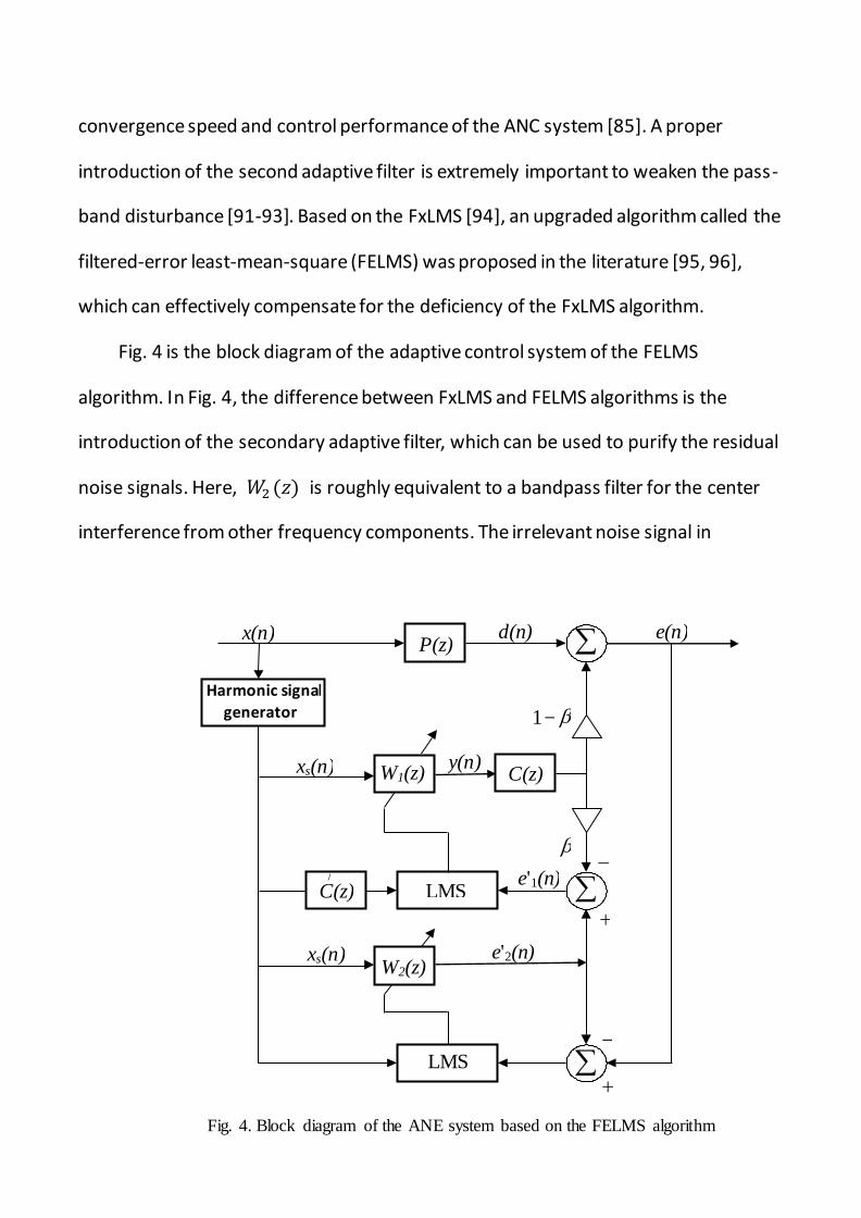
convergence speed and control performance of the ANC system [85]. A proper

introduction of the second adaptive filter is extremely important to weaken the pass-

band disturbance [91-93]. Based on the FxLMS [94], an upgraded algorithm called the

filtered-error least-mean-square (FELMS) was proposed in the literature [95, 96],

which can effectively compensate for the deficiency of the FxLMS algorithm.

Fig. 4 is the block diagram of the adaptive control system of the FELMS

algorithm. In Fig. 4, the difference between FxLMS and FELMS algorithms is the

introduction of the secondary adaptive filter, which can be used to purify the residual

noise signals. Here, 𝑊2 (𝑧) is roughly equivalent to a bandpass filter for the center

interference from other frequency components. The irrelevant noise signal in

P(z)

LMS

/ C(z)

C(z)

x(n)

Harmonic signal generator

1

LMS

W2(z)

W1(z)

d(n) e(n)

y(n)

xs(n)

xs(n)

e'1(n)

e'2(n)

Fig. 4. Block diagram of the ANE system based on the FELMS algorithm

𝑒(𝑛) is significantly reduced when 𝑒(𝑛) is filtered by the adaptive filter 𝑊2 (𝑧).

Furthermore, instead of 𝑒(𝑛), the output signal 𝑒2′ (𝑛) is entered into the adaptive

filter 𝑊1 (𝑧), which produces the error signal 𝑒1′ (𝑛). 𝑒1

′ (𝑛) is used to update the

weight vector of the adaptive filter 𝑒1′ (𝑛) to maintain the convergence speed and

control performance of the system.

Simulations are divided into two parts. The first part verifies the superiority of

FELMS algorithm compared to FXLMS algorithm. The simulation has been done for

the FELMS and FXLMS algorithms under the same conditions and environments. The

calculation results show that the FELMS algorithm provides better control

performance and faster convergence than the FxLMS algorithm due to the secondary

adaptive filter in the FELMS algorithm. While in the second part, the simulation is

conducted with 𝑓1 = 50𝐻𝑧, 𝑓2 = 100𝐻𝑧, 𝑓3 = 200𝐻𝑧, and different gain values

(β < 2). The input signal 𝑥(𝑛) is the combination of the three sine waves with the

same power. The simulation result shows that the FELMS algorithm can effectively

control the residual noise spectrum by different gain settings, without affecting

neighbour components.

Another variant of the ANE algorithm is the Normalization equalizer filtered-x

LMS (NEX-LMS) algorithm, which was developed in [77]. In this algorithm, a

normalization filter is added to offer better convergence ability than the ANE

algorithm with limited computational complexity.

3.3 SF-cFxLMS algorithm

A simplified Fx-LMS (SF-FxLMS) algorithm was proposed in [97], which enables

one to estimate the relationship between the psychoacoustic analysis results and the

parameters of the disturbance. Then, Jaime introduced the complex-domain data to

improve the stability of the SF-FxLMS algorithm in response to impulsive

disturbances, and developed the SF-cFxLMS algorithm (simplified-form complex

FxLMS) [98].

In Fig. 5, the residual noise is measured by the error microphone in the SF-

cFxLMS ANC system and written as

𝑒(𝑛) = 𝑑(𝑛) − 𝑦(𝑛) = 𝑑(𝑛) − 𝑆(𝑧)[𝑊𝑙+1𝑇 (𝑛)𝑥(𝑛)] (5)

where y(n) is the control actuation that superimposes with the primary disturbance

d(n), S(z) is the real secondary path, Wl+1(n) is the adaptive weight vector and x(n) is a

normalized reference signal. Based on the NEX-LMS strategy [77], the estimated

primary disturbance �̂�(𝑛) is [99]:

�̂�(𝑛) = 𝑒(𝑛) + �̂�(𝑧)[𝑊𝑙+1𝑇 (𝑛)𝑥(𝑛)] (6)

The Fastest Fourier Transform in the West (FFTW) is used to calculate �̂�(𝑛);

then, the first (N/2+1) bins are retrained for subsequent operations. The amplitude

and relative-phase (block of “Amp/Rel. Phase” in Fig. 5) of the desired components

can be estimated as follows:

�̂�𝑘 (𝑙) = ℱ[�̂�(𝑛)] = ℱ ([�̂�0(𝑛)�̂�1(𝑛) ⋯ �̂�𝐿−1(𝑛)]𝑇

)

= [�̂�𝐷𝐶 (𝜔)�̂�1(𝜔) ⋯ �̂�𝑁/2(𝜔)]𝑇 (7)

Similar to �̂�(𝑛), 𝑒(𝑛) and 𝑥′(𝑛) are estimated as follows:

𝐸𝑘′ (𝑙) = [𝑒𝐷𝐶 (𝜔)𝑒1(𝜔) ⋯ 𝑒𝑁/2(𝜔)]

𝑇 (8)

𝑋𝑘′ (𝑙) = [𝑥𝐷𝐶 (𝜔)𝑥1(𝜔) ⋯ 𝑥𝑁/2(𝜔)]

𝑇 (9)

Fig. 5. Block diagram of the SF-cFxLMS ANC system

From Fig. 5, 𝐸𝑘′ (𝑙) = 𝐸𝑘 (𝑙) − �̂�𝑘 (𝑙) and 𝑥′(𝑛) = �̂�(𝑧) ∗ 𝑥(𝑛) are calculated. Then,

after the updating operations ([98] Section 3), the missing complex conjugate part can

be calculated from the updated (N/2+1) weights. Therefore, the weight vector

𝑊𝑙+1(𝑛) is obtained as follows:

𝑊𝑙+1(𝑛) = ℱ−1[𝑊𝑙+1(𝜔)] = ℱ−1([𝑊𝐷𝐶 (𝜔)𝑊1(𝜔) ⋯ 𝑊𝑁 (𝜔)]𝑇) (10)

Eq. (10) is the weight update equation of the SF-cFxLMS algorithm. It is useful to

reduce the computational burden and improve the stability of the updating algorithm;

thus, the control signal is generated by the adaptive controller:

𝑢(𝑛) = 𝑊𝑙+1𝑇 (𝑛)𝑥(𝑛) (11)

Computer simulations for controlling the sound quality of low frequency based

on loudness and roughness were conducted. Capabilities such as the independent

control of a number of narrowband components with a single adaptive filter,

adequate convergence speed and an improved convergence procedure face to

impulsive disturbances are thoroughly demonstrated through different computer

simulation scenarios [98]. Furthermore, the SF-cFxLMS algorithm can emerge as a

promising control scheme, as sound quality targets can be achieved with the

implementation of the proposed algorithm, even if the disturbance is contaminated

with broadband noise.

In the continued study [100], Jaime’s group introduced the Multiple-Input,

Multiple-Output (MIMO) arrays [101,102] and established the MIMO ASQC system,

which compensated for the amplitude and relative phase interferences, while

retaining an active effect on the SQ metrics, namely, Loudness and Roughness.

3.4 CMD algorithm

Based on the principle of minimal disturbance [103], the constrained minimal

disturbance (CMD) algorithm was proposed by Walter J Kozacky [104]. In this study,

constraints are added to limit the filter gain, filter convergence, and filter output

power. Then, the Lagrange multiplier [105] method, which helps the CMD algorithm

obtain a faster convergence speed, is used to solve the constrained optimization

problem [106]. Fig. 6 shows the input, weight, and error vectors of the CMD adaptive

filter, which are given by

Fig. 6. Block diagram of the CMD adaptive filter with frequency-domain processing

𝑥(𝑚) = [𝑥(𝑛)𝑥(𝑛 − 1) ⋯ 𝑥(𝑛 − 𝑁 + 1)]𝑇

𝑤(𝑚) = [𝑤0(𝑛)𝑤1(𝑛 − 1) ⋯ 𝑤𝑁−1(𝑛)]𝑇

𝑒(𝑚) = [𝑒(𝑛)𝑒(𝑛 − 1) ⋯ 𝑒(𝑛 − 𝑁 + 1)]𝑇 (12)

where N is the block size; m is the block iteration. By updating m in each block, the

weight vectors are updated using the CMD algorithm, which can minimize the

squared Euclidean norm of the frequency domain weight change. The equation is

𝑊𝑘 (𝑚 + 1) = 1 − 𝜇𝛾𝑘 𝑊𝑘(𝑚) + 𝜇𝑘 𝑆𝑘∗(𝑚)𝑋𝑘

∗(𝑚)𝐸𝑘(𝑚) (13)

where 𝜇 is the convergence step size; 𝛾𝑘 =𝛼𝑘

𝜇(1+𝛼𝑘); 𝛼𝑘 is a Lagrange multiplier. By

taking the IFFT (Inverse Fast Fourier Transform) on both sides of Eq. (13) and casting

into a delay-less structure, we obtain the new algorithm

𝑆∗(𝑚)𝑋∗(𝑚)

S(m)

E(m)

IFFT

S ( z )

FFT

Delay

x(n)

FFT

×

) ( z W

µ

FFT

×

y(n)

d(n)

e(n) ys(n)

×

𝑤(𝑚 + 1) = 𝑤(𝑚) + 𝜇𝐼𝐹𝐹𝑇{𝑆∗ (𝑚)𝑋∗(𝑚)𝐸(𝑚)

𝑆(𝑚)2 𝑋(𝑚) 2− 𝛤(𝑚)𝑊(𝑚)} (14)

where 𝛤(𝑚) is a diagonal matrix of variable leakage factors.

(14) is called the weight update equation of the CMD algorithm. The simulations

verify the superiority of the CMD algorithm compared to the leaky LMS algorithm in

both power-constrained and gain-constrained applications. The frequency response

and convergence of the two algorithms are compared in the power-constrained

simulation. The CMD algorithm provides faster convergence performance than the

leaky LMS algorithm and maintains a 6 dB power reduction over frequency. The CMD

algorithm allows the power constraint to be set explicitly, while the leaky LMS

algorithm requires a trial and error approach to determine the parameters. In the

gain-constrained simulation, the CMD algorithm has better frequency response

performance and faster convergence than the leaky LMS algorithm, particularly in

coloured noise environments [104].

3.5 PSC-FxLMS algorithm

The phase scheduled command FXLMS (PSC-FXLMS) algorithm, which was

proposed by Rees and Elliott [107], uses an internal model to obtain an estimate of

the disturbance signal [89,108]. The block diagram of PSC-FXLMS is shown in Fig. 7

[107].

Fig. 7. Block diagram of the PSC-FxLMS algorithm

In Fig. 7, the error signal can be written as

𝑒(𝑛) = 𝑑(𝑛) + 𝑔𝑇𝑢(𝑛) (15)

𝑒′(𝑛) = 𝑒(𝑛) − 𝑐(𝑛) (16)

where 𝑔𝑇 is the impulse response vector, 𝑐(𝑛) is a command signal. The filter

weight 𝑤(𝑛) of PSC-FXLMS algorithm can be updated as

𝑤(𝑛 + 1) = 𝑤(𝑛) − 𝜇�̂�(𝑛)𝑒′(𝑛) (17)

where 𝜇 is the step size and �̂�(𝑛) is the filtered reference signal vector. The

disturbance signal �̂�(𝑛) is estimated by plant model �̂�(𝑧), and �̂�(𝑛) can be

expressed as

�̂�(𝑛) = 𝑒(𝑛) − 𝑔𝑇𝑢(𝑛) = 𝑑(𝑛) + 𝑔𝑇𝑢(𝑛) − 𝑔𝑇𝑢(𝑛) (18)

Furthermore, 𝑢(𝑛) is dependent on 𝑐(𝑛), since 𝑢(𝑛) = 𝑤(𝑛)𝑥(𝑛), then the

�̂�(𝑧)

𝑐𝑜𝑠( 𝜔𝑟 𝑇𝑛)

c(n)

�̂�(𝑧)

G(z)

FFT

Signal

Generator

x(n)

W(z)

×

𝜙𝑑

d(n)

e(n)

u(n)

�̂�(𝑛)

𝑒′(n) r̂(n)

update weight equation for a single filter coefficient can be written as

𝑤(𝑛 + 1) = 𝑤(𝑛) − 𝜇�̂�(𝑛)𝑒′(𝑛) = 𝑤(𝑛) − 𝜇�̂�(𝑛)[𝑑(𝑛) + 𝑔𝑇𝑢(𝑛) − 𝑐(𝑛)] (19)

Then, Rees and Elliott incorporated automatic phase command technique into PSC-

FXLMS algorithm to deal with the problem of phase instability when large system

gains are needed.

Experimental Sound profiling of a tone was conducted under the condition of a

pure 1000 rad (159.16 Hz) tone at a sample rate of 16 samples per period (2.55 kHz)

[107]. Experimental results show that the control effort is not excessive when the

output is enhanced. The properties of the command-FXLMS algorithm, the internal

model FXLMS algorithm, and the PSC-FXLMS algorithm were evaluated, including: the

convergence speed, the stability, and the control effort. The command-FXLMS is

stable due to the simplicity of the algorithm, but it has excessive control effort. The

internal model FXLMS is stable at low gains, and it requires low values of control

effort relative to the command-FXLMS. The PSC-FXLMS shows not only to achieve

those modes of control capable by the internal model FXLMS with increased gain

accuracy, but also with an increase in stability to plant model magnitude errors.

In the continued study [109], Patel and Cheer introduced the MPSC-FxLMS

algorithm which allows the phase of the disturbance signal to be detected directly

without the need for an additional internal plant model.

3.6 ANNs algorithm

Artificial neural networks (ANNs) recently became a forceful candidate for active

noise cancellation [110-114], particularly for the system identification with active

vibration control [115] and nonlinear dynamic problems [116-122]. ANNs, which have

been used to model the relationship between subjective and objective evaluations,

can describe an annoyance model with a non-stationary noise signal [123-125].

The structure of the ANNs system in [126] is shown in Fig. 8. The outputs of

ANNs are the objective rate of sound quality; if it has great correlation with the

subjective rate, the outputs of the ANNs become a good sound quality index.

Fig. 8. Structure of ANNs for the noise index: (a) single neuron i; (b) three-layer, back-propagation

(BP) network

The main purpose of the ANNs algorithm is to map an input vector x ∈ 𝑅𝑁 into

the output vector y ∈ 𝑅𝑀 , which can be written as:

𝑥𝑁×1 → 𝑦𝑀×1 (20)

In general

𝑥(𝑝) → 𝑦(𝑝) , and p=1, 2, 3,…, k (21)

where k is the number of patterns. The network performs this mapping, which

consists of processing neurons and their connections. The ith single neuron is shown

in Fig. 8(a); the input signals xj are cumulated in a neuron-summing block Σ and

export the only output yi via function F:

𝑦𝑖 = 𝐹(𝑧𝑖), 𝑧𝑖 = ∑ 𝑤𝑖𝑗𝑁𝑗=𝑖 𝑥𝑗 + 𝑏𝑖 (22)

where zi is the potential parameter, wi ,j is the weight of connection, and bi is the

threshold parameter. The sigmoid function can be written as:

𝐹(𝑧) =1

1+𝑒−𝜇𝑧𝜖(0,1) for µ>0 (23)

A standard multiplayer network of the input, hidden and output layers is shown

in Fig. 8(b). In this figure, N = 4 is the number of inputs; H1 = 5, and H2 = 3 are the

numbers of neurons in their respective hidden layers; M = 2 is the number of outputs

in the output layer. This network can be called the 4–5–3–2 structure network. In this

structure, the biases 𝑏𝑖𝑙 and weights 𝑤𝑖,𝑗

𝑙 (where 𝑙 is the number of layers) are the

network’ parameters [125]. Mathematically, the sound quality index using 𝑏𝑖𝑙 and

𝑤𝑖,𝑗𝑙 is written by

Sound quality index = 𝐹2[𝐿𝑤2𝐹1(𝐼𝑤1𝑥 + 𝑏1) + 𝑏2] (24)

where function F follows the form of Eq. (23), Iw1 and Lw2 are the weight matrices of

the input layer and the first hidden layer. The trained ANNs were applied to

investigate the characteristics of the interior sounds [121-125]. The calculation results

show that the output of the trained ANNs has the significant correlation with the

averaged subjective rating of sounds. It is concluded that the output vector of the

ANNs can objectively estimate the rate of noise sound. Eq. (24) can be used as a

design guide for sound quality with sufficient accuracy and reliability to improve the

human subjective satisfaction [123].

4. Selective attenuation method for the ASQC-based ANC scheme

Selective attenuation methods were recently used in ANC schemes [39,126-129],

which can reduce the sound pressure level and adjust the sound characteristics. The

frequency selective least-mean-square (FSLMS) algorithm has been shown in [39] to

be an effective candidate towards the desired selective noise control target; it

simultaneously properly eliminates the dysphoric composition and retains the

element of pleasure [130].

Fig. 9 is the block diagram of the FSLMS algorithm, where the awaiting

cancellation of the original signal is given by:

𝑑(𝑛) = 𝑑1(𝑛) + 𝑑2(𝑛) (25)

where x (n) is strongly correlated with d (n), after x (n) is filtered by H(z), x'(n) is

related to d1(n), but x'(n) and d2(n) are irrelevant.

Fig.9. Block diagram of the FSLMS algorithm

Based on the LMS algorithm and the relevant cancellation principle, input,

H(z)

LMS

W(z)

x́(n) x(n) y(n)

d(n)

e(n)

output, error vector, and weight of the FSLMS adaptive filter are given by:

𝑥′(𝑛) = ℎ(𝑛) ∗ 𝑥(𝑛) (26)

𝑦(𝑛) = 𝑊𝑇(𝑛)𝑥′(𝑛) = �̂�1(𝑛) (27)

𝑒(𝑛) = 𝑑(𝑛) − 𝑦(𝑛) = 𝑑(𝑛) − �̂�1(𝑛) ≈ 𝑑2(𝑛) (28)

𝑤(𝑛 + 1) = 𝑤(𝑛) + 2𝜇𝑒(𝑛)𝑥′(𝑛) (29)

where (29) is the weight update equation of the FSLMS algorithm, which is relatively

near the autocorrelation matrix eigenvalue of signal x'(n), and its convergence

condition is:

0 < 𝜇 <1

𝐸[𝑥′ (𝑛)2 ] (30)

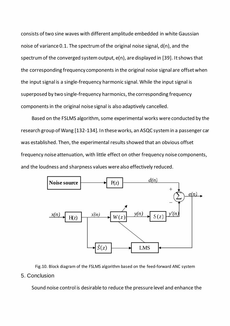
The FSLMS algorithm based on the feed-forward ANC scheme [131], as shown in

Fig. 10, must be considering the effect of the secondary-channel sound delay on the

algorithm stability. By imitating the derivation process of the FxLMS algorithm, the

equations of the FSLMS algorithm based on the feed-forward ANC scheme are given

by:

𝑦(𝑛) = 𝑊𝑇 (𝑛)𝑥′(𝑛) (31)

𝑊(𝑛 + 1) = 𝑊(𝑛) − 2𝜇𝑒(𝑛)𝑟(𝑛) (32)

𝑟(𝑛) = 𝑥′(𝑛) ∗ ℎ2(𝑛) = ℎ(𝑛) ∗ 𝑥(𝑛) ∗ ℎ2(𝑛) (33)

where 𝑟(𝑛) is the input signal of the weight coefficient iterative updating. In Fig. 10,

𝑟(𝑛) is obtained from the input signal 𝑥(𝑛) and filtered by 𝐻(𝑧) and �̂�(𝑧).

In practical applications, a multiple FSLMS system can be configured in parallel to

cancel the residual noise spectrum when the original noise has multiple harmonics.

The simulation was conducted with M=16, step size µ=0.002. The original noise signal

consists of two sine waves with different amplitude embedded in white Gaussian

noise of variance 0.1. The spectrum of the original noise signal, d(n), and the

spectrum of the converged system output, e(n), are displayed in [39]. It shows that

the corresponding frequency components in the original noise signal are offset when

the input signal is a single-frequency harmonic signal. While the input signal is

superposed by two single-frequency harmonics, the corresponding frequency

components in the original noise signal is also adaptively cancelled.

Based on the FSLMS algorithm, some experimental works were conducted by the

research group of Wang [132-134]. In these works, an ASQC system in a passenger car

was established. Then, the experimental results showed that an obvious offset

frequency noise attenuation, with little effect on other frequency noise components,

and the loudness and sharpness values were also effectively reduced.

Fig.10. Block diagram of the FSLMS algorithm based on the feed-forward ANC system

5. Conclusion

Sound noise control is desirable to reduce the pressure level and enhance the

P ( z )

LMS

) ( z S

Noise source

) ( z W x́(n)

H ( z ) y’(n) x(n)

d(n)

e(n)

y(n)

�̂�(𝑧)

auditory qualities of sound fields. The paper has introduced the concept of sound

quality, objective evaluation, subjective evaluation and their relationships. Then, we

reviewed the active noise control methods with an emphasis on recent developments

in sound quality enhancement, which is briefly shown in Table 1. This paper can serve

as a reference or a tutorial for beginners in the field of ASQC.

Table 1 Main characteristic of active sound quality control.

Authors Algorithms Characteristic Reference

Kuo ANE Attenuate or amplify sinusoidal noise [83,84]

Kuo / Bao FELMS Introduce the secondary adaptive filter to

weaken the pass-band disturbance

[95,96]

Sun/Jaime SF-cFxLMS Estimate the relationship between psychoacoustic analyses results and the

parameters of the disturbance

[97,98]

Walter CMD Provide faster convergence and improve

frequency response performance

[104]

Rees and Elliott PSC-FxLMS Increase the gain accuracy and the stability

of the phase errors

[107]

Lee et al. ANNs Sound quality index [123-125]

Jiang and Wang FSLMS Eliminate the dysphoric composition and retain

the element of pleasure

[39]

Acknowledgment

The financial support of the China Scholarship Council [grant 201607585012] is

gratefully acknowledged.

References

[1] Lu Xiaojun, Wang Dengfeng. Infrasound test system and infrasound vs test means

of human body physiology function effect. Acta Acustica,2002, 27（1）：27-32.

[2] Nithin V.George, GanapatiPanda. Advances in active noise control: A survey, with

emphasis on recent nonlinear techniques. Signal Processing 2013; 93: 363–377.

[3] WANG Deng-feng, LIU Zong-wei, LIANG Jie. Subjective evaluation experiments and

objective quantificational description of vehicle interior noise quality. Journal of

Jilin University (Engineering and Technology) 2006; 2: 343–353.

[4] J. Blauert. Product-sound assessments: An enigmatic issue from the point of view

of engineering. Proc. internoise94, Yokohama, Japan, 1994; 2: 857-862.

[5] U Jekosch. Meaning in the context of sound quality assessment. Acta Acustica 1999;

85(5): 681-684.

[6] Jiao F L, Liu K. Sound quality in noise control:Ⅱ Subjective assessment [A].

Proceedings of 2003 National Conference Environmental Acoustics [C]. 2003.

[7] Franz K. Brandl, Werner Biermayer. A new tool for the on board objective

assessment of vehicle interior noise quality. SAE Paper 1999; 01: 1695.

[8] Kousuke Noumura, Junji Yoshida. Perception modeling and quantification of sound

quality in cabin. SAE paper 2003; 01: 1514.

[9] Lijian Zhang. A sensory approach to develop product sound quality criterion. SAE

Paper 1999; 01: 1818.

[10] Norm Otto, Scott Amman, Chris Eaton, Scott Lake. Guidelines for jury evaluations

of automotive sounds. SAE Paper 1999; 01: 1822.

[11] M. Van Auken, J. W. Zellner and D. T. Kunkel. Correlation of Zwicker’s loudness and

other noise metrics with driver’s over-the-road transient noise discomfort. SAE

Paper 1998; 05: 85.

[12] Scott A. Amman, Mike A. Blommer. Psychoacoustic considerations in vehicle

ergonomic design. SAE Paper 1999; 01: 1269.

[13] Jun Lu, Jay Pyper, Ronald Weber, Jonathan Fisk. Windshields with new PVB

interlayer for vehicle interior noise reduction and sound quality improvement. SAE

Paper 2003; 01: 1587.

[14] Seon-Yang Hwang, Koo-Tae Kang, Byung-Soo Lim, Yoon-Soo Lim. Noise reduction

and sound quality improvement of valve train in V6 gasoline engine. SAE Paper

2005; 01: 1834.

[15] Quehl J. Comfort studies on aircraft interior sound and vibration [D]. Carl-von-

Ossietzky University Oldenburg; 2001.

[16] Jie Pan, Roshun Paurobally, Xiaojun Qiu. Active noise control in workplaces. Acoust

Aust 2016; 44: 45–50.

[17] Patsouras Ch. Psychoacoustic evaluation of tonal components in view of sound

quality design for high speed train interior noise. Acoustical Science &Technology

2004; 23(2): 113-116.

[18] Vos J. Annoyance caused by magnetic levitation train transrapid 08-a laboratory

study [M]. TNO Report; 2003.

[19] Jeon J Y，You J，Kim Y. S. Evaluation of sound quality of air-conditioning Noise

[A]. Proceeding of The 9th Western Pacific Acoustic Conference [C]. Seoul, Korea;

2006.

[20] Jin Yong Jeon. Sound radiation and sound quality characteristics of refrigerator

noise in real living Environments. Applied Acoustics 2006; 06: 005.

[21] Cong Zhang. Subjective evaluation of sound quality for mobile spatial digital

audio. 2008 International Conference on Computer Science and Software

Engineering, p: 250-253.

[22] Ishiyama T, Hashimoto T. The impact of sound quality on annoyance caused by

road traffic noise: an influence of frequency spectra on annoyance. JSAE Review,

21：225-230.

[23] Yang W, Kang J. Acoustic comfort evaluation in urban open public spaces. Applied

Acoustics 2005; 66: 211-229.

[24] Mutsumi Ishibashi, Anna Preis, Fumiaki Satoh, Hideki Tachibana. Relationships

between arithmetic averages of sound pressure level calculated in octave bands

and Zwicker’s loudness level. Applied Acoustics 2006; 67: 720-730.

[25] Nicola Prodi, Sylvia Velecka. The evaluation of binaural playback systems for virtual

sound fields. Applied Acoustics 2003; 64: 147-161.

[26] C. M. Harris. Handbook of acoustical measurements and noise control. New York;

1991.

[27] Xu Yongcheng, Wen Xisen, Chen Xun. An overview on active noise control

technology and application. Journal of National University of Defense Technology.

2001; Vol.23 (No.2): 119-124.

[28] S.M. Kuo, D.R. Morgan. Active noise control systems: algorithms and DSP

implementations. New York: Wiley; 1996.

[29] Lueg P. Process of silencing sound oscillations [P]. United States, Patent 2043416,

1936.

[30] H.F. Olson, E.G. May. Electronic sound absorber. Journal of the Acoustical Society

of America 1953; 25 (6): 1130–1136.

[31] Liu Enze, Yan Jikuan, Chen Duanshi. Survey and development trend of active

noise control system. Noise and Vibration Control 1999; 3: 2-6.

[32] Nelson P A, Elliott S J. Active control of sound [M]. Academic Press, London;

1992.

[33] Manpeil Tamamura, Eiji Shibata. Application of active noise control for engine

related cabin noise. JSAE Review 1996.

[34] Jerome Couche. Active control of automobile cabin noise with conventional and

advanced speakers. Master thesis, Virginia 1999.

[35] B. Widrow, S.D. Stearns. Adaptive signal processing, prentice-hall. Engle Wood

Cliffs, NJ 1985.

[36] F. Russo, G.L. Sicuranza. Accuracy and performance evaluation in the genetic

optimization of nonlinear systems for active noise control. IEEE Transactions on

Instrumentation and Measurement 2007; 56 (4): 1443–1450.

[37] M.A. Sahib, R. Kamil. Comparison of performance and computational complexity

of nonlinear active noise control algorithms. ISRN Mechanical Engineering 2011:

1–9.

[38] M. G. Larimore, J. R. Treichler, C. R. Johnson. SHARF: An algorithm for adaptive IIR

digital filters. IEEE Trans. Acoust, Speech, Signal Processing 1980; vol. ASSP-28:

428–440.

[39] Jiang Ji-guang, Wang Deng-feng. Active control of vehicle interior noise based on

selective attenuation method. Second International Conference on Information

and Computing Science. Manchester, UK; 2009.

[40] Joachim Scheuren, Ulrich Widmann, Jens Winkler. Active noise control and

sound quality design in motor vehicles. SAE Paper 1999; 01: 1846.

[41] A. Gonzalez, M. Ferrer, M. de Diego, G. Pinero, J. J. Garcia-Bonito. Sound quality

of low-frequency and car engine noises after active noise control. Journal of

Sound and Vibration 2003; 265: 663-679.

[42] M. de Diego, A. Gonzalez, G. Pinero, M. Ferrer, J. J. Garcia-Bonito. Subjective

evaluation of actively controlled interior car noise. Acoustics, Speech, and Signal

Processing; 2001.

[43] Sen M. Kuo, Ravi K. Yenduri. Frequency-domain delay less active sound quality

control algorithm. Journal of Sound and Vibration 2008; 318: 715–724.

[44] Chambers J, Bullock D, Kahana Y, Kots A, Palmer A. Developments in active noise

control sound systems for magnetic resonance imaging. Applied Acoustics 2007;

68:281–95.

[45] Hua Bao, Issa M.S. Panahi. Psychoacoustic active noise control with ITU-R 468

noise weighting and its sound quality analysis. 32nd Annual International

Conference of the IEEE EMBS Buenos Aires, Argentina, August 31 - September 4;

2010.

[46] R.R. Leitch, M.O. Tokhi. Active noise control system. IEEE Proceedings Part A 134

1987; 6: 525–546.

[47] S.J. Elliott, P.A. Nelson. Active noise control. IEEE Signal Processing Magazine

1993; 4: 12–35.

[48] S.M. Kuo, D.R. Morgan. Active noise control: a tutorial review. Proceedings of the

IEEE 1999; 6: 943–975.

[49] Nikhil Cherian Kurian, Kashyap Patel, Nithin V. George. Robust active noise

control: An information theoretic learning approach. Applied Acoustics 2017;

117: 180–184.

[50] Liu Zongwei, Wang Dengfeng, Liang Jie. Research and advance meat on subjective

evaluation and improvement of vehicle interior noise quality. Automobile

Technology 2006; 7: 1-4.

[51] Rossi F, Nicolini A, Filipponi M. An index for motor vehicle passengers acoustical

comfort. The 32nd international congress and exposition on noise control

engineering Korea; 2003.

[52] Bodden M. Instrumentation for sound quality evaluation. Acustica 1997; 83: 775-

783.

[53] E. Zwicker, H. Fastl. Psychoacoustics. Facts and Models, Second Ed. Springer-

Heidelberg, Berlin, Germany; 1999.

[54] Wang Dengfeng, Liu Xueguang, Liu Zongwei. Layout experiment of secondary

sound source for adaptive active noise control system in vehicle interior. China

Journal of Highway and Transport 2006; 19(3): 122-126.

[55] B&K, Lecture Note, Introduction to sound quality, 2004.

[56] Acoustics: Method for calculating loudness level. ISO532-1975.

[57] Procedure for calculating loudness level and loudness. DIN45631-1991.

[58] Bismarck, V. Sharpness as an attribute of the timbre of steady sounds. Acoustica

1974; 30: 159-172.

[59] Aures, W. The sensory euphony as a function of auditory sensations. Acoustica

1985; 58: 282-290.

[60] Jiang Ji-guang, Wang Deng-feng. Objective evaluation model for interior sound

quality research. Third International Conference on Modelling and Simulation.

June 4–5, China, 2010.

[61] Aures, W. A procedure for calculating auditory roughness. Acoustica 1985; 58: 268-

281.

[62] Zwicker, E., Fastl, H. Psychoacoustics: Facts and Models, second. Springer Verlag,

Berlin; 1999.

[63] Mao Dong-xing, ZHANG Bao-long. Performance of semantic differential method

with an anchor stimulus in subjective sound quality evaluation. Technical

Acoustics 2006; 25(6): 560-567.

[64] Altinsoy E, Kanca G, Belek HT. A comparative study on the sound quality of wet-

and-dry type vacuum cleaners. The sixth international congress on sound and

vibration, Denmark; 1999.

[65] Osgood C E, Tannenbaum P H, Suci G J. The measurement of meaning [M]. Urbana:

University of Illinois Press, 1957.

[66] Schulte-Fortkamp B. The quality of acoustic environments and the meaning of

soundscapes [A]. Proceedings of the 17th International Congress on Acoustics [C].

Rome, Italy; 2001.

[67] Hashimoto T, Hatano S. Effect of factors other than sound to the perception of

sound quality. Proceedings of the 17th International Congress on Acoustics [C].

Rome, Italy; 2001.

[68] Zeitler A, Hellbrück J. Semantic attributes of environmental sounds and their

correlations with psychoacoustic magnitudes. Proceedings of the 17th

International Congress on Acoustics [C]. Rome, Italy; 2001.

[69]David, H.A. The method of Paired Comparisons, 2nd London, Chapman and Hall,

1988.

[70] Mohd Jailani Mohd Nor, Mohammad Hosseini Fouladi, Hassan Nahvi, Ahmad

Kamal Ariffin. Index for vehicle acoustical comfort inside a passenger car. Applied

Acoustics 2008; 69: 343–353.

[71] S.J. Elliott. Signal Processing for active control. Academic Press, San Diego, Calif.;

London, 2001.

[72] Y.-S. Lee, S. J. Elliott. Active position control of a flexible smart beam using

internal model control. Journal of Sound and Vibration 2011; 242(5): 767–791.

[73] D. Bismor. LMS algorithm step size adjustment for fast convergence. Archives of

Acoustics 2012; 37(1): 31-40.

[74] Feng Liu, James K. Mills, Mingming Dong, Liang Gu. Active broadband sound

quality control algorithm with accurate predefined sound pressure level. Applied

Acoustics 2017; 119: 78–87.

[75] L.P.R. de Oliveira, K. Janssens, P. Gajdatsy, H. van der Auweraer, P.S. Varoto, P. Sas,

W. Desmet. Active sound quality control of engine induced cavity noise.

Mechanical Systems and Signal Processing 2009; 23: 476–488.

[76] J. Cheer, S. J. Elliott. Multichannel control systems for the attenuation of interior

road noise in vehicles. Mech. Syst. Signal Process. 2015; 60: 753–769.

[77] L.P.R. de Oliveira, B. Stallaert, K. Janssens, H. van der Auweraer, P. Sas, W.

Desmet. NEX-LMS: a novel adaptive control scheme for harmonic sound quality

Control. Mechanical Systems and Signal Processing 2010; 24: 1727–1738.

[78] Lee HH, Lee SK. Objective evaluation of interior noise booming in a passenger car

based on sound metrics and artificial neural networks. Applied Ergonomics 2009;

40(5): 860–869.

[79] J.A. Mosquera-Sánchez, J.D. Villalba, L.P.R. de Oliveira. A multi-objective

optimization procedure for guiding the active sound quality control of

multiharmonic disturbances in cavities. Proceedings of Internoise 2013.

[80] J.A. Mosquera-Sánchez, W. Desmet, K. Janssens, L.P.R. de Oliveira. Towards sound

quality metrics balance on hybrid powertrains. Proceedings of ICED 2015.

[81] C.A. Powell, B.M. Sullivan. Subjective response to propeller airplane interior

sounds modified by hypothetical active noise control systems. Noise Control

Engineering Journal 2001;49 (3): 125–136.

[82] H. Bao, I. Panahi. Using A-weighting for psychoacoustic active noise control. Proc.

Int. Conf. IEEE Eng. Med. Biol. Soc., Vancouver, British Columbia, Canada; 2009:

5701-5704.

[83] Kuo SM, Ji MJ. Principle and application of adaptive noise equalizer. IEEE Trans

Circuits Systems II: Analog Digital Signal Process 1994; 41: 471–4.

[84] Kuo SM, Ji MJ. Development and analysis of an adaptive noise equalizer. IEEE

Trans Speech Audio Process 1995; 3: 217–222.

[85] Deng-feng Wang, Ji-guang Jiang, Zong-wei Liu, Xiao-lin Cao. Research on ANE

algorithm for sound quality control of vehicle interior noise. 3rd International

Conference on Information and Computing 2010; 107-110.

[86] Feng JW, Gan WS. Adaptive active noise equalizer. IEEE Electronics Letters 1997;

33(18), 1518-1519.

[87] Kuo SM, Yajie Y. Broadband adaptive noise equalizer. IEEE Signal Process 1996; 3:

234-235.

[88] Feng J, Gan W-S. A broadband self-tuning active noise equalizer. Signal Process

1997; 62: 251-256.

[89] Jinxin Liu, Xuefeng Chen. Adaptive compensation of mis-equalization in

narrowband active noise equalizer systems. IEEE/ACM Transactions on Audio,

Speech, and Language Processing 2016; 24(12):2390-2399.

[90] Gonzalez A, de Diego M, Ferrer M, Pinero G. Multichannel active noise

equalization of interior noise. IEEE Trans Audio, Speech, Language Process 2006;

14: 110-22.

[91] S. M. Kuo, M. Tahernezhadi, L. Ji. Frequency-domain periodic active noise control

and equalization. IEEE Transactions on Speech and Audio Processing 1997; 05,

348-358.

[92] S. M. Kuo, M. J. Ji. Pass band disturbance reduction in adaptive narrowband noise

control systems. IEEE Transactions on Circuits System I 1999; 46: 220-223.

[93] S. Mallu. Integration and optimization of active noise equalizer with filtered error

least mean square algorithm. MS Thesis, Northern Illinois University 2005.

[94] Seokhoon Ryu, Yun Jung Park, Young-Sup Lee. Active suppression of narrowband

noise by multiple secondary sources. Journal of Sensors 2016: 1-9.

[95] S.M. Kuo, J. Tsai. Residual noise shaping technique for active noise control

systems. J. Acoustical Soc. America, 1994; 95(3): 1665-1668.

[96] Hua Bao, Issa M.S. Panahi. A perceptually motivated active noise control design

and its psychoacoustic analysis. ETRI Journal 2013; 35(5): 859-868.

[97]X.Sun, G.Meng. LMS algorithm for active noise control with improved gradient

estimate. Signal Process 2006; 20: 920–938.

[98] Jaime A. Mosquera-Sánchez, Leopoldo P.R. de Oliveira. A multi-harmonic

amplitude and relative-phase controller for active sound quality control.

Mechanical Systems and Signal Processing 2014; 45: 542–562.

[99]B.Farhang-Boroujeny. Adaptive filters: theory and applications. John Wiley & Sons

England; 1998.

[100] Jaime A. Mosquera-Sánchez, Wim Desmet, Leopoldo P.R. de Oliveira. A

multichannel amplitude and relative-phase controller for active sound quality

control. Mechanical Systems and Signal Processing 2017; 88: 145–165.

[101] J.A. Mosquera-Sánchez, K. Janssens, W. Desmet, L.P.R. de Oliveira. Multichannel

active sound quality control for independent-channel sound profiling. Euro noise

2015.

[102] Jaime A. Mosquera-Sánchez, Wim Desmet, Leopoldo P.R. de Oliveira.

Multichannel feed forward control schemes with coupling compensation for

active sound profiling. Journal of Sound and Vibration 2017; 396: 1–29.

[103] S Haykin. Adaptive filter theory. Prentice-Hall, Upper Saddle River, NJ, 2002.

[104] Walter J Kozacky, Tokunbo Ogunfunmi. An active noise control algorithm with

gain and power constraints on the adaptive filter. EURASIP Journal on Advances

in Signal Processing 2013:17.

[105] R Fletcher, Practical Methods of Optimization. New York, Wiley: 1987.

[106] WJ Kozacky, T Ogunfunmi. Convergence analysis of a frequency-domain

adaptive filter with constraints on the output weights. Conference on Signals,

Systems, and Computers USA, 2009: 1350–1355.

[107]L. E. Rees, S. J. Elliott. Adaptive algorithms for active sound-profiling. IEEE/ACM

Transaction on Audio, Speech and Language Processing, 2006; 14(2), 711-719.

[108] Chuansheng Xiao, Fengyan An. Stability analysis of broadband active noise

equalization algorithm. Proceedings of 20th International Congress on Acoustics,

23-27 August 2010, Sydney, Australia.

[109] Vinal Patel, Jordan Cheer. Modified phase-scheduled-command FxLMS

algorithm for active sound profiling. IEEE/ACM Transaction on Audio, Speech and

Language Processing, 2017; 25(9), 1799-1808.

[110] Q.Z. Zhang, X.D. Li, W.S. Gan. Active noise control using a simplified fuzzy neural

network. Journal of Sound and Vibration 2004; 272: 437-449.

[111] Y.L. Zhou, Q.Z. Zhang, X.D. Li, W.S. Gan. Analysis and DSP implement of an ANC

system using a filtered-error neural network. Journal of Sound and Vibration

2005; 285: 1-25.

[112] Lee SK, Kim TG, Lim JT. Characterization of an axle-gear whine sound in a sports

utility vehicle and its objective evaluation based on synthetic sound technology

and an artificial neural network. Proc I Mech E Part D: J Automobile Engineering

2008; 222(3): 383–396.

[113] Lee SK, Kim BS, Park DC. Objective evaluation of the rumbling sound in

passenger cars based on an artificial neural network. Proc I Mech E Part D: J

Automobile Engineering 2005; 219(4): 457–469.

[114] S.K. Lee, H.C. Chae, D.C. Park, S.G. Jung. Sound quality index development for

the booming noise of automotive sound using artificial neural network

information theory. Sound Quality Symposium 2002, Michigan USA, CD N0.5.

[115] P.Q. Xia. An inverse model of MR damper using optimal neural network and

system identification. Journal of Sound and Vibration 2003; 266: 1009-1023.

[116] S. Tomasiello. An application of neural networks to a nonlinear dynamics

problem. Journal of Sound and Vibration 2004; 272: 461-467.

[117] J.C. Patra. Chebyshev neural network-based model for dual- junction solar cells.

IEEE Transactions on Energy Conversion 2011; 26 (1): 132–139.

[118] J.C. Patra, P.K. Meher, G. Chakraborty, Nonlinear channel equalization for

wireless communication systems using Legendre neural networks. Signal

Processing 2009; 89 (11): 2251–2262.

[119] N.V. George, G. Panda. A reduced complexity adaptive Legendre neural network

for nonlinear active noise control. Proceedings of the 19th International

Conference on Systems, Signals and Image Processing 2012: 560–563.

[120] J.C. Patra, P.K. Meher, G. Chakraborty. Development of Laguerre neural-

network-based intelligent sensors for wireless sensor net- works. IEEE

Transactions on Instrumentation and Measurement 2011; 60 (3): 725–734.

[121] D.P. Das, G. Panda, Active mitigation of nonlinear noise processes using a novel

filtered-s LMS algorithm. IEEE Transactions on Speech and Audio Processing

2004; 12 (3): 313–322.

[122] J.C.Patra, R.N.Pal, B.N.Chatterji, G.Panda. Identification of nonlinear dynamic

systems using functional link artificial neural networks. IEEE Transactions on

Systems, Man, and Cybernetics—Part B: Cybernetics 1999; 29(2): 254–262.

[123] Eui-Youl Kim, Tae Jin Shin, Sang Kwon Lee. New tonality design for non-

stationary signal and its application to sound quality for gear whine sound.

Journal of Automobile Engineering 2013; 227(3): 311-322.

[124] Lee HH, Kim SK, Lee SK. Design of new sound metric and its application for

quantification of an axle gear whine sound by utilizing artificial neural network. J

Mechanical Science and Technology 2009; 23(4):1182-1193.

[125] Sang-Kwon Lee. Objective evaluation of interior sound quality in passenger cars

during acceleration. Journal of Sound and Vibration 2008; 310: 149-168.

[126] S. Hu, R. Rajamani, X. Yu. Active noise control for selective cancellation of

eternal disturbances. 2011 American Control Conference on O'Farrell Street, San

Francisco, CA, USA June 29 - July 2011; 01: 4737-4742.

[127] Marco Bergamasco, Fabio Della Rossa, Luigi Piroddi. Active noise control of

impulsive noise with selective outlier elimination. 2013 American Control

Conference Washington, DC, USA, 2013; 4165-4170.

[128]EmmanuelA. Ntumy, SergeyV. Utyuzhnikov. Active sound control in composite

regions. Applied Numerical Mathematics 2015; 93: 242–253.

[129]K.V.Devara. Active noise cancelling headset and devices with selective noise

suppression, Patent WO2002082422 A2, 2002.

[130] Liu Zong-wei, Wang Deng-feng, Liang Jie. Study and development of subjective

evaluation of inner noise quality and improvement. Automobile Technology

2006; 7: 1-4.

[131] Joplin P M, Nelson P A. Active control of low frequency random sound in

enclosures. J. Acoust. Soc. Am. 1990; 87: 2396-2404.

[132] Jiang Jiguang, Wang Dengfeng. Research on active control of vehicle interior

noise based on selective attenuation method. Science Technology and

Engineering 2014; 12: 288-291.

[133] Jiang Ji-guang, Wang Deng-feng. Subjective and objective evaluation of vehicle

interior noise sound quality preference and correlation research. Automotive

Technology 2012; 8: 6-10.

[134] Ji-guang Jiang. Adaptive active control system of vehicle noise design and test.

2014 2nd World Congress on Industrial Materials Application, Products, and

Technologies 2014:251-256.