JOURNAL OF GEOPHYSICAL RESEARCH, VOL. 105, NO. C6, PAGES 14,197-14,213, JUNE 15, 2000

Tide at the eastern section of the Strait of Gibraltar

Jesds Garcia Lafuente, Juan Miguel Vargas, Francisco Plaza, and Tarek Sarhan

Departamento de F•sica Aplicada II, University of Malaga, Malaga, Spain

Julio Candela

Centro de Investigaci6n Cient•fica y Educaci6n Superior de Ensenada, Ensenada Baja California M•xico

Burkard Bascheck

Institut fiir Meerskunden,University of Kiel, Kiel, Germany

Abstract. From October 1995 to April 1996, three mooring lines were deployed at the eastern entrance of the Strait of Gibraltar. The spatial coverage of the mooring array allows for a good description of the tides. They exhibit a dominant semidiurnal nature and a noticeable baroclinic structure that matches the one of the

mean exchange. Tidal currents in the upper layer are irregular and usually too weak to reverse the mean upper layer flow that keeps on flowing east. Lower layer flow reverses with semidiurnal periodicity because of the smallness of the mean flow and the appreciable amplitude of the regular semidiurnal oscillation of tidal currents in this layer. Tidal transports can be satisfactorily compared with previous estimates of Bryden et al. [1994] if we allow for strong internal divergences associated with the internal tide. No significant eddy flux of water transport (tidal rectification) is observed at the eastern section, contrary to the almost 50% of the total layer transport found by Bryden et al. [1994] in Camarinal Sill section. Time-dependent hydraulic theory provides a good scenario for interpreting these two independent sets of observations despite the fact that the composite Froude number does not reach the critical values predicted in the hydraulic models most of the time.

1. Introduction

The Strait of Gibraltar, which connects the Atlantic Ocean and the Mediterranean Sea through a rather complicated system of sills and narrows, is the sce- nario of a well-studied baroclinic exchange between two basins with different densities. The driving force is the net loss of freshwater in the Mediterranean Sea due to

the excess of evaporation over precipitation and river runoff. Relatively fresh Atlantic water (SA -• 36.2 in the practical salinity scale) is ultimately transformed in salty water of SM "• 38.5 that leaves the Mediter- ranean Sea as an undercurrent whose influence extends

far away from the strait in the Atlantic Ocean [Reid, 1979].

The long-term averaged inflow of Atlantic water, QA, and outflow of Mediterranean water, QM (QM < 0), must satisfy two conservative laws for mass (Q• +QM = E) and salt (Q.•$.• + QMSM = 0) budgets in the Mediterranean Sea. These relations could be used to

Copyright 2000 by the American Geophysical Union.

Paper number 2000JC900007. 0148-0227/00/2000JC900007509.00

estimate Q• and Q M if the net evaporative rate E in the Mediterranean Sea and the salinity of the Mediter- ranean water, $M, were known. The uncertainty of the value of E along with the fact that $M itself de- pends implicitly on E make the estimates of Q A and Q M vary over a wide range of values [Lacombe and Tch- ernia, 1972; Bethoux, 1979; Lacombe and Richez, 1982; Bryden and Kinder, 1991]. Recent estimates of the ex- changed flows using direct currentmeter observations taken during the Gibraltar Experiment give a value of -•0.7 Sv (1 Sv-10 6 m3s -1) for both inflow and outflow [Bryden et al., 1994] (hereinafter referred to as BCK94), a flow smaller than those traditionally reported.

The complex bottom topography of the strait and the fact that sills are to the side of the Atlantic Ocean, the reservoir of light water, with reference to the narrowest section, provide suitable conditions for the existence of a hydraulically controlled baroclinic exchange. This hy- pothesis was analyzed by Armi and Farmer [1985] from historical data. They developed the necessary theoreti- cal background for a steady two-layer hydraulic theory that implies maximal exchange between the connected basins [Farmer and Armi, 1986]. The candidate loca- tions for control are the narrowest section off Tarira and

14,197

14,198 GARCIA LAFUENTE ET AL.' STRAIT OF GIBRALTAR EASTERN SECTION TIDE

the areas of minimum cross-area and minimum depth of Camarinal Sill (see Figure 1). composite Froude number

At the controls the

G 2=F•+F•= u•l + u• (1) g• h • g• h•

2/g/h i is the internal is critical (G 2--1). Here Fi • - u i Froude number of layer i, whose velocity and depth are ui and hi, respectively, g/ - g(p2- Pl)/P• is the re- duced gravity, and pi is the layer density. Bryden and Kinder [1991] applied this theory to the Strait of Gibral- tar to estimate flows using realistic topography and to force the flows to satisfy the aforementioned conserva- tive laws. Their predictions agree within 20% with the observations for the accepted values of E.

These mean flows are strongly influenced by tides. Vertical tide behaves basically as a standing wave with amplitudes increasing toward the Atlantic [Garci•a La- fuente et al., 1990]. Internal oscillations have much greater amplitudes. Petrigrew and Hyde [1990] reported semidiurnal changes of 200 m in the depth of the inter- face during spring tides off Tarifa. Tidal flow through the strait is basically nonlinear. The formation of in- ternal hydraulic jumps west of Camarinal Sill almost every tidal cycle, their release near the end of the ebb when tidal currents weaken, and the large interface os- cillations produced by their subsequent propagation are

36.3

36.2 - SPAIN

-6.0 -5.9 -5.8 -5.7 -5.6 -5.5 -5.4 -5.3 LONGITUDE

Figure 1. Map of the Strait of Gibraltar show- ing the positions of the mooring lines (crosses) and conductivity-temperature-depth (CTD) stations (cir- cles). Some topographic features are shown: CS is Ca- marinal Sill, TN is Tarifa Narrows, TB is Tangier Basin, and WES is West Espartel Sill. The isobaths are 100 m (labeled), 290 m, which is the contour of the light shaded area, and 400 m, which is the contour of the medium shaded area. The remaining lines correspond to 500, 700, and 900 m and have not been labeled to keep the map clear.

the most archetypal signatures of nonlinearities [Armi and Farmer, 1988; Farmer and Armi, 1988]. However, this cannot be the only contribution to the observed os- cillations since during many neap tides, bores are not released [Armi and Farmer, 1988; Farmer and Armi, 1988; Watson and Robinson, 1990], yet the interface os- cillates. Tidal currents are the most energetic phenom- ena in Camarinal Sill and in many other areas of the strait [Lacombe and Richez, 1982; Candela et al., 1990, hereinafter referred to as CWR90]. Strikingly, there are other places where tides appear to be of secondary im- portance. For instance, the outflow through the west- ernmost sill of the strait (West Espartel Sill, see Figure 1) show little tidal variability [Armi and Farmer, 1988; Farmer and Armi, 1988]. The inflow through the east- ernmost exit of the strait behaves similarly (CWR90; this work).

Farmer and Armi [1986] incorporated tides into the hydraulic model using a quasi-steady approximation in which the steady solution is verified at each point of the tidal cycle. Hellrich [1995] showed that this approach is only valid for dynamically short straits, a concept related to the parameter • = (g/hl)•/2T/L that mea- sures the length L of the strait relative to the distance an internal signal will travel during the forcing period T. The quasi-steady approximation is only valid for • -• c•. Both theories predict an increase of the ex- changed flows with the strength of the barotropic tidal forcing through tidal rectification, but they differ in the amount of rectified transports. The quasi-steady theory always predicts more flow than the time-dependent the- ory. BCK94 found that •50% of the exchanged flows through Camarinal Sill crossed the section as a bolus of water because of the positive correlation between currents and interface oscillations. This percentage is above the predictions of either theory for the represen- tative parameters of the Strait of Gibraltar. The time- dependent theory predicts a dependence of the instanta- neous transports on the location of the section because it allows for internal divergences associated with nonin- stantaneous internal adjustment.

This work aims at describing the tides at the east- ern section of the strait and determining whether their spatial patterns may be interpreted in the frame of hy- draulic models, which seem adequate for studying the exchange. Section 2 presents the data set and data processing as well as a criterion for choosing the in- terface. Section 3 describes the spatial structure of the tides at the eastern section and investigates dynamic balances in an unidimensional model. Finally, section 4 compares our estimates with BCK94 results and sum- marizes our conclusions.

2. Data and Methods

From October 1995 to April 1996, two mooring lines of conventional (Aanderaa) currentmeters were deployed by the University of M•laga (mooring N, see Figure 1)

GARCIA LAFUENTE ET AL.: STRAIT OF GIBRALTAR EASTERN SECTION TIDE 14,199

and the Institut fiir Meereskunde (mooring S) in the eastern section of the Strait of Gibraltar as part of the pilot phase of the Canary Islands Azores Gibraltar Ob- servations (CANIGO) project. A third line (mooring C) was deployed by Woods Hole Oceanographic Insti- tution within another U.S. Office of Naval Research

supported project. Mooring locations as well as other information of interest are presented in Table 1. In June 1997 the CANIGO-JUNE 97 survey took place in the Strait of Gibraltar onboard the R/V Cornide de $aavedra from the Instituto Espafiol de Oceanograf•a (IEO). Conductivity-temperature-depth (CTD) profiles were made at each of the stations shown in Figure 1 during more than 20 hours, with a sampling interval of ..•1 hour, in order to investigate internal semidiurnal tidal oscillations. Hourly sea level data of the Span- ish ports of Algeciras, Tarira, and Ceuta were also col- lected. These data are the experimental basis of the present study. Other currentmeter observations in the southern and center sites, not simultaneous with these analyzed here, and a set of CTD casts in the positions of moorings N and C have also been used to help resolve some particular questions.

2.1. Salinity Corrections and Isohaline Depths

Currentmeters were equipped with temperature, con- ductivity, and pressure sensors. Salinity is then readily obtained at the different sampling depths. Conductiv- ity cells of these types of instruments drift to unrealis- tically low values as time goes by because of biological contamination of the cell. Therefore salinity series have the same trend. The closer to the surface the instru-

ment is, the more accentuated the drifting because of the enhanced biological activity in the photic layer. Un-

fortunately, upper instruments are necessary to depict the vertical motions of the isohalines, and so, a method to correct these drifts was devised. The approach is described by Garcia Lafuente et al. [1998] and takes advantage of the fact that, because of the length of the mooring line, instruments nominally in the upper layer are eventually dragged down to the lower one by the strong spring tidal currents (see Figure 2). Here they should record temperature and salinity of Mediter- ranean water, which has rather constant values of 13øC and 38.4, respectively. While temperature sensors do work correctly, conductivity cells start drifting after some weeks, making the computed salinity smaller than expected. A time subseries of salinity (or conductivity) taken when temperature has Mediterranean values al- lows us to estimate salinity (or conductivity) drift and to correct it from the whole series.

The corrected time series were used to estimate the

isohaline depth by linear interpolation. When the salin- ity recorded by the uppermost instrument exceeded the value So of the selected isohaline, its depth cannot be determined. In these cases we have used boundary con- ditions inspired in the S(z) diagrams of the whole set of CTD casts accomplished in sites N and C, which are shown in Figure 3a and Figure 3b. The vahies S=36.6 at z=0 m and S=36.5 at z=-25 m were assumed for

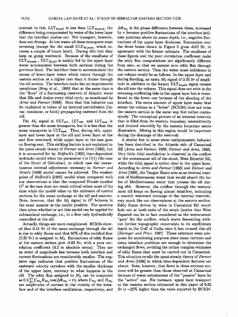
moorings N and C, respectively, and used to make in- terpolation in these infrequent situations. An example of the depth of $0-37.2 in mooring C is presented in Figure 4b. Currentmeters in mooring S were well be- low the isohalines of interest (salinity in station S1 was always >38.3) so that no computations have been done here. Linear extrapolations of estimates in sites N and C have been used instead.

Table 1. Currentmeter Information

Station Nominal Depth Bin Size, Percentage Latitude, Longitude, Start Stop Water Depth, (nd), m m o N o W m

N1 30 nd- 50 76.3 36ø02.4 5ø23.7 24.10.95 08.05.96 450 N2 60 nd-80 80.6 36ø02.4 5ø23.7 24.10.95 08.05.96 450 N3 120 nd-140 83.2 36ø02.4 5ø23.7 24.10.95 08.05.96 450 N4 250 nd-270 80.1 36ø02.4 5ø23.7 24.10.95 08.05.96 450 N5 410 nd-420 92.4 36ø02.4 5ø23.7 24.10.95 08.05.96 450 C1 32 nd-58 77.1 35ø59.7 5ø23.2 17.10.95 18.04.96 925 C2 53 nd-79 77.5 35ø59.7 5ø23.2 17.10.95 18.04.96 925 C3 a 74 nd-100 77.7 35ø59.7 5ø23.2 17.10.95 18.04.96 925 C4 108 nd-133 79.0 35ø59.7 5ø23.2 17.10.95 18.04.96 925 C5 158 nd-181 78.9 35ø59.7 5ø23.2 17.10.95 18.04.96 925 C6 263 nd-290 85.2 35ø59.7 5ø23.2 17.10.95 18.04.96 925 C7 765 nd-805 84.0 35ø59.7 5ø23.2 17.10.95 18.04.96 925 S1 410 nd-445 79.4 35ø57.1 5ø21.5 17.10.95 08.05.96 700

S2 610 b ... 35ø57.1 5ø21.5 17.10.95 08.05.96 700

The second column is the nominal depth of each station, the third column is the bin size (see text), and the fourth column is the percentage of data inside the bin.

•The rotor of this instrument stopped working correctly after December 13, 1995. bThis currentmeter was not equipped with a pressure sensor. Station S1 has been used for reference.

14.200 GARCIA LAFUENTE ET AL.: STRAIT OF GIBRALTAR EASTERN SECTION TIDE

0 •:

..400 •, • ____• , 300 3.50 400 4.5.0

Day from January f, Y995

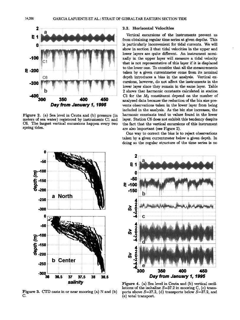
Figure 2. (a) Sea level in Ceuta and (b) pressure (in meters of sea water) registered by instruments C1 and C6. The largest vertical excursions happen every two spring tides.

2.2. Horizontal Velocities

Vertical excursions of the instruments prevent us from obtaining regular time series at given depths. This is particularly inconvenient for tidal currents. We will show in section 3 that tidal velocities in the upper and lower layers are quite different. An instrument nomi- nally in the upper layer will measure a tidal velocity that is not representative of this layer if it is displaced to the lower one. To consider that all the measurements

taken by a given currentmeter come from its nominal depth introduces a bias in the analysis. Vertical ex- cursions, however, do not affect the instruments in the lower layer since they remain in the same layer. Table 2 shows that harmonic constants calculated in station

C1 for the M2 constituent depend on the number of analyzed data because the reduction of the bin size pre- vents observations taken in the lower layer from being included in the analysis. As the bin size increases, the harmonic constants tend to values found in the lower

layer. Station C6 does not exhibit this tendency despite the fact that the vertical excursions of this instrument

are also important (see Figure 2). One way to correct the bias is to reject observations

taken by a given currentmeter below a given depth. In doing so the regular structure of the time series is no

. . 0 . • . •.,• . -50 ........... . '--½-- •:.

ß . '

450 .......... : ........... ' ........... : ........ .

ß

-200 .......... • ............ : ........................ ß . .

a North

-250 l' ' -300

O -f .• •, . . .

. . t..V ,,.,4 -50 " t .'• - ' ß -- .,,v ...k..' $: X, ,

.......... • ....... ,.•.%' '•. • ,•_,• -100 .... 450 .......... • ........................ :..',":,-',' ß .

-200 '• ' ß

b Center ' -250 '

-300 ...... 36 36.5 37 37.5 38

sal/n/• 38.5

Figure 3. CTD casts in or near mooring (a) N and (b) C.

E 1 !!'":':' "•"- ': ';::":"•'.'":'::,.::- '•"• •'""'"'"'"":'"' :" ß •. ...< • .

• -100• ..... :: .... .,:.., "'"':. •.;•!'::'i ':-:-•!::,. ::'..:'. • •.:::'-;.... ..... :..• -•-" ,,- ,. :..;.:-• •.:,.• : . .•. •* . :: • • • • :,•

• 2 •'::'::•':"'•'- .... •,:.. ......... , .............................. ß ............ • ß .... . .:- . .:. :

.'::,• :•.:':•::' • ::. '.•,. ½. :.::'?;..,: : 4, ,:-...,,-.½: ........ . ....... .. ,

. - , •.4 • ß ....: :-. . • .., •. •::a.,• : .. ;•.. .;.. ..... : ...½.. ., :s . .: . :•: • • 'i: ..:s .:•.•: '* .;:: ;• :': .. ";" •.::.• ; •: .:. ' :. • .• ::s•: •:. • ..... ...--.. . ..... -:.•..• •. .,.•::•..½ .... .

•-• & .......... '•

300 350 40.0 450

Day from

Figure 4. (a) Sea level in Ceuta and (b) vertical oscil- lations of the isohaline S=37.2 in mooring C, (c) trans- ports above S=37.2, (d) transports below S=37.2, and (e) total transport

GARCIA LAFUENTE ET AL.' STRAIT OF GIBRALTAR EASTERN SECTION TIDE 14,201

Table 2. Test of Data From Stations C1 and C6

Station C1 Station C6

Bin % A a g 0 A a g 0

35-58 m 77.1 14.7 -3.7 14 244 42.6 3.6 23 131 35-80 m 90.6 19.3 -2.1 18 210 42.7 3.6 23 131

35-100 m 94.6 21.1 -1.4 17 200 42.9 3.6 23 131 35-140 m 98.2 22.8 -0.6 16 193 43.0 3.7 23 131 35-180 m 99•3 23.2 -0.4 16 191 43.2 3.7 23 131 All data i00 23.5 -0.4 16 191 43.2 3.7 23 131

M2 Harmonic constants in C1 and C6. A and a are major and minor semiaxes in cm s -x, g is the inclination of the major semiaxis, anticlockwise from east, and 0 is the phase lag in degrees referred to the moon transit by Greenwich meridian. Harmonic constants on each row are obtained using only data taken in the moments in which instrument C1 was inside the bin specified in the first column. The second column gives the percentage of data inside the bin.

longer preserved, and the new time series is unevenly spaced. This is not important for estimating harmonic constants by least squares fitting if the rejected observa- tions are randomly distributed in time. This is not the case since spring tidal periods account for most of the rejected data, which introduces a new bias because of the limited amount of data during these periods. Table 2 shows, however, that 77% of observations with this biased distribution provide good estimates of harmonic constants for M2 in station C6, for which we choose the first alternative. Consequently, each currentmeter is associated with a bin that contains at least 75% of the observations. This is indicated in column 3 of Table 1.

Bins of stations C1 and C2 and C2 and C3 necessarily overlap a few meters in order to maintain the threshold of 75% of observations within each of them.

2.3. Transport Estimates

In a reference system with the x axis oriented along the strait (rotated 17 ø anticlockwise from east), the y axis oriented across the strait, positive northward, and the z axis positive upward, the transports above and below an internal surface whose depth is H(y, t) at time t are computed according to

ULT(t) = u(y, z, t)dzdy (2a) =o

•w z=•/(u,t) LLT(t) -- f --0 J z--bottom

u(y,z,t)dzdy (2b)

where u(y, z, t) is the along-strait component of the ve- locity, W is the width of the strait and ULT and LLT are upper layer transport (above the internal surface) and lower layer transport (below the internal surface), re- spectively. NET-ULT+LLT is the total transport that does not depend on the internal surface used to compute (2a) and (2b). In practice, the along-strait component

of the velocity is obtained from currentmeter observa- tions. Equations (2a) and (2b) are transformed in

3 0

ULT(t) = ••1 • ui(z,t)dz (3a) ø____. -----Hi

3

LLT = ••1 • ui(z,t)dz (3b) ß _ ----bottom

where subindex i refers to the three subareas in which

the whole cross-area of the section has been divided.

Figure 5 shows the shape of the mooring section adapted from the topographic map by $anz et al. [1991] and the three subareas. Currentmeter observations in each

mooring are considered as representative for the corre- sponding sub-area, and Hi(t), the depth of the selected

-250

s -oo

-750

-1000 0 2 4 8 8 10 12 14 16 18

Across-Strait distance (kin)

Figure 5. Cross-area of the eastern section and the three subareas into which it has been divided to carry out computations.

14,202 GARCIA LAFUENTE ET AL.: STRAIT OF GIBRALTAR EASTERN SECTION TIDE

0.95

0.9

0.85

0.8 37 37.3 37.6 37.9 38.2

Salinity Figure 6. Transport above a given isohaline as a func- tion of its salinity. The solid line is a third-degree poly- nomial fitting to the computed transports.

isohaline in the mooring position at time t, is taken as constant for the subarea. Integrals in (3a) and (3b) have been replaced by summations. Along-strait veloc- ity was determined in the center of a bin 10 m thick in each subarea by means of linear interpolation or ex- trapolation, and the integral was readily evaluated. The condition u=2 m s -1 at z=-5 m was imposed whenever the extrapolated velocity at this depth exceeded 2 m S --1 '

Mooring S, with only two instruments, lacked infor- mation in the upper layer. The gap was filled using currentmeter observations from stations C1, C2, C3, and C4 to generate time series at the same levels in site S. It was done using regression coefficients obtained by means of correlation analysis of simultaneous time series in C and S acquired between July and October 1997. After this, mooring S was processed in the same manner as moorings N and C. An example of transport estimated using $o=37.2 is presented in Figures 4c, 4d and 4e.

2.4. Interface Depth

The interface between inflow and outflow would be

defined as the internal surface where zero along strait velocity occurs. This obvious definition must be com- mented upon, however. Instantaneous velocities are dominated by tidal currents that are strong enough to reverse inflow or outflow during certain phases of the tides, as happens, for instance, in Camarinal Sill sec- tion (CWR90 and BCK94). In addition, inflow does not consist of Atlantic water uniquely, neither does out- flow consist uniquely of Mediterranean water. Bray et al. [1995] showed that the more to the east the sec- tion is, the saltier (on average) both inflow and outflow are, and the more to the west the section is, the freshet both inflow and outflow are. The reason is that east

of the sill, the fast flowing "Atlantic" Jet entrains part of the out,owing Mediterranean water that is forced to recirculate into the Mediterranean, thus increasing the size of the inflow and its salinity. West of the sill, the fast flowing "Mediterranean" undercurrent entrains At- lantic water, which increases the size of the outflow but decreases its salinity.

It is convenient to define an isohaline that plays the role of interface in order to investigate tidal transports since the definition above makes no sense when the flows

reverse. The numerical value of this isohaline changes from one section to the other in the strait. BCK94 gave consistent reasons to accept $=37.0 as the interface in Camarinal Sill, but this is a rather low value in the eastern section. CWR90 used $=37.2 to carry out some calculations here.

To identify the best isohaline to represent the inter- face in the eastern part, transports defined by (2a) and (2b) have been maximized. It is obvious that their sizes depend on the internal surface used as limit in the in- tegral. Figure 6 shows the transport above a given iso- haline as a function of its numeric value. Since the

net transport is independent of the choice of the iso- haline, it is also representative of the transport below

-100 -so

-200

-250

37.2

37. 7 ........ 3•.0 .... :' ' "• "• ............. :':•::' ' : •' ' ' ':•:'•'":'" ' '•'::•' ' ' ':• ..... •::•' ' ..........

• ::¾•:: i "• .:•: '• • .?:•:..- . ß v' • • :•::•.....•:-:.- . ß • ...•- • •:• ..... • .... , • '-.r • . • • ........ • .

..... 38.1 "•

300 320 340 360 380

Day from J-anua 1995 Figure 7. Low-frequency vertical oscillations of some isohalines (thin solid lines) and depth of the zero velocity of low-frequency flow (thick line) in mooring C. The shaded area represents the layer bound by $=37.7 and $=38.0.

GARCIA LAFUENTE ET AL.: STRAIT OF GIBRALTAR EASTERN SECTION TIDE 14,203

Table 3. Percentage of Variance (Energy) in the Different Frequency Bands

Station Low-Frequency Diurnal Semidiurnal High-Frequency Band % Band % Band % Band %

(f < 0.025 cph) (0.025 < f • 0.50 cph) (0.050 • f • 0.11 cph) (f > 0.11 cph)

All stations (average) 18.5 7.6 60.0 13.9 C2 34.4 9.3 37.4 18.9 N4 3.5 4.9 86.0 5.6 S1 1.4 7.4 88.8 2.1

Upper Layer (average) 35.0 10.0 35.0 20.0 Lower Layer (average) 5.0 5.0 85.0 5.0

The first row gives a weighted average (weights being proportional to the cross area the station represents) for all stations. Rows 2-4 give the distribution of energy in three selected stations, one from each mooring. The last two rows show estimates of the percentage of the variance in the upper and lower layers.

that surface. The curve peaks at S=37.85 so that inflow and outflow are maxima for this value. Consequently, this should be considered the interface. This value is

in good agreement with the three-layer exchange model put forward by Bray et al. [1995], in which the interfa- cial layer of intermediate salinities was flowing eastward at the eastern section.

Figure 7 shows subinertial depth variations of some isohalines and of the surface of the zero along-strait ve- locity in mooring C. Subinertial variability is not great enough to reverse flows so that the last surface defines unambiguously the interface. It fluctuates around the depth of S=37.85, supporting the choice of this isoha- line as the interface (in fact, the isohaline whose mean depth coincides with the mean depth of the surface of zero along-strait velocity is S=37.81). The close cor- respondence between the isohalines and the zero veloc- ity surface oscillations, the latter lagging the former, is noteworthy.

3. Results

3.1. General Remarks

Table 3 summarizes some general results about the spatial distribution of velocity variance (energy). The first row shows that most of the energy is located in the semidiurnal frequency band, confirming that semidiur- nal tides dominate the flow variability. Low-frequency (subinertial) motions follow in importance and then high-frequency motions and diurnal tides. However, the local distribution of energy is different. The second row of Table 3 shows that the percentage of energy in semi- diurnal and subinertial bands is comparable in C2, a representative station of the Atlantic layer. Rows 3 and 4 show the partition of energy for stations N4 and S1, confirming that the most energetic phenomenon in the lower layer in this section is, by far, the semidiurnal tide. The last two rows give an average distribution of energy in both layers. There is a clear asymmetry that seems to be related to the mean baroclinic exchange.

The spatial structure of tidal currents in general and of semidiurnal currents in particular is also typically baroclinic.

One way of estimating quantitatively the importance of barotropic and baroclinic contributions to the to- tal tide is by means of empirical orthogonal functions (EOFs) that assign energy to different empirical modes orthogonal to each other. We have isolated the semi- diurnal frequency band with a bandpass filter made as the difference of two low-pass, order 7, butterworth fil- ters with half power points at 0.6 and 0.1 cph, respec- tively. Table 4 and Figure 8 show the results of the application of the EOF analysis to the filtered series. The real part of the spatial weights, which corresponds to the along-strait component of the velocity, is plotted in Figures 8a and 8b for the first and second empir- ical modes (modes have been sorted according to the variance they explain). The first mode does not invert sign and can be identified with a barotropic mode. The second mode inverts sign around the mean interface of the zero along-strait velocity and can be interpreted as the first baroclinic mode. Table 4 gives the amount of semidiurnal energy in each station and how much of it resides in each mode. The last column indicates that

these two modes account for most of the energy, and therefore they provide an acceptable representation of the semidiurnal tides. The second empirical mode pre- vails in stations of the upper layer, while the first em- pirical (barotropic) mode explain more than 90% of the energy in stations of the lower layer. These stations have more variance in absolute terms than stations of

the upper layer, which indicates stronger tidal currents.

3.2. Harmonic Constants

Table 5 gives harmonic constants for the most im- portant constituents of semidiurnal and diurnal bands. Constituent Z0 is included to help locate the different stations in either layer (see the Table 5 caption). Sta- tions C4 and N3 have near-zero amplitude for Z0 and must have been close to the interface, sometimes above

14,204 GARCIA LAFUENTE ET AL.: STRAIT OF GIBRALTAR EASTERN SECTION TIDE

Table 4. Variance in the Semidiurnal Band

Station Variance M • Percentage M•, Percentage M(x +•,), %

N1 a 435 66 15.2 285 65.4 80.6 N2 a 372 190 51.0 67 18.1 69.1 N3 764 620 81.1 23 2.9 84.0 N4 1360 1308 96.2 15 1.1 97.3 N5 1224 1122 91.6 51 4.2 95.8 C1 • 685 32 4.7 614 89.8 94.5 C2 • 628 10 1.6 593 94.4 96.0 C4 420 314 74.8 17 4.0 78.8 C5 609 562 92.3 I 0.2 92.5 C6 958 923 96.3 4 0.4 96.7 C7 937 901 96.2 0 0.0 96.2 S1 721 694 96.2 I 0.1 96.3 S2 722 695 96.3 3 0.4 96.7

The second column shows the amount of variance (cm s -•') in each station. Columns 3 and 4 are the variance accounted for the first empirical mode (cm s -•') and its percentage, respectively. Columns 5 and 6 are the same for the second empirical mode. The last column is the percentage of variance explained by both modes. Station C3 has not been included in this analysis because of its reduced length.

• Stations in the upper layer.

0

-250

-5OO

-250

-500

-750

-1000 0 3 6 9 12 15 18

Across-Strait distance (km)

figure 8. Spatial weights of (a) the first and (b) second empirical modes for the semidiurnal frequency band. The shaded area indicates the cross section for the mean

inflow as given by Z0 constituents at the different sta- tions.

it and sometimes below it, since the position of the interface fluctuates. This could be the reason for the anomalous value of some harmonic constants evaluated

there.

3.2.1. Semidiurnal currents. The spatial struc- ture of M2 shown in Figure 9a and Figure 9b corre- sponds well with the spatial structure of Z0, the mean flow, and matches the baroclinic structure discussed above. The amplitudes and phases remain almost con- stant below the interface of zero velocity (unshaded area), while they vary quickly as we move upward into the upper layer (shaded area). Table 5 shows that the sense of rotation of the velocity vector along the tidal ellipse changes from one layer to the other, a typical baroclinic feature. Phases around 130 ø in the lower-

layer stations are coherent with the vertical tide whose phase at the eastern part of the strait is 47.5 ø [Garcia La/uente et al., 1990], because of the standing wave na- ture of semidiurnal oscillations in the Strait of Gibral-

tar. They are also consistent with the value of 140 ø given by CWR90 in Camarinal Sill. CWR90 showed that more than 80% of the energy (variance) of the semi- diurnal currents in the sill is coherent with the sea level

oscillation. Therefore M2 tidal currents in the lower layer of the eastern section are barotropic. On the con- trary, the lack of agreement in the upper layer can only be explained by the presence of an important baroclinic component. Another example of the influence of this component is provided by the phase difference between $2 and M2 that defines the age of the tide or the time difference between the largest range of spring tide and the occurrence of the full or new moon. It is i day (•30 ø) in the lower layer, the same as in the verti- cal tide [Garcia Lafuente et al., 1990]. CWR90 also showed a stable difference of phase of --30 ø through- out the water column in Camarinal Sill. The phase difference 852 -8M2 in stations of the upper layer has a negative mean (stronger semidiurnal currents before

GARCIA LAFUENTE ET AL.: STRAIT OF GIBRALTAR EASTERN SECTION TIDE 14,205

Table 5. Harmonic Constants for M2, $2, and K1

St Z0 M•. S•. Kx

A g A a g O A a g O A a g O

N1 ' 40.9 10 11.9 -5.3 26 226 6.1 0.3 36 183 10.8 -3.6 21 124 N2 ' 12.5 -11 13.7 -2.8 37 155 6.0 -0.7 24 167 7.6 -2.8 24 98 N3 1.9 177 30.4 -2.1 23 116 10.3 -1.3 19 148 4.0 1.3 15 48 N4 12.0 206 50.2 1.2 28 130 16.2 0.3 29 163 10.0 -0.1 9 36 N5 8.0 266 48.1 -2.0 29 128 11.7 1.1 32 151 9.6 0.1 27 24 C1 ' 87.3 4 14.7 -3.7 14 244 7.9 -1.4 2 222 10.9 -2.5 -7 157 C2 ' 58.1 2 17.3 -4.6 14 247 6.6 -1.1 -1 212 10.1 -3.6 -7 146 C3 ' 25.8 -3 7.1 -0.1 18 205 4.9 -2.4 23 201 7.1 -4.1 -3 119 C4 1.8 -20 17.8 0.1 -1 127 7.5 -0.9 9 160 5.7 0.6 25 61 C5 16.0 193 31.1 1.2 10 128 10.1 -0.5 9 156 6.7 1.9 18 45 C6 23.3 206 42.6 3.7 23 131 14.3 1.4 21 162 8.5 0.8 25 49 C7 16.2 213 43.0 0.4 21 133 13.5 0.6 24 161 9.26 -0.7 22 48 S1 4.7 173 35.2 1.8 9 133 9.5 0.5 5 164 8.3 -0.1 8 34 S2 4.7 196 37.1 0.8 2 126 11.6 .2 3 158 6.8 -0.8 16 31

Amplitudes, inclination, and phases are as in Table 2. Negative values of a mean clockwise rotation. Mean current (Z0 constituent) is included to show the close relationship between the spatial structure of the mean flow and the main tidal constituents. Stations N3 and C4 appear to have been close to the interface of zero mean velocity.

'Stations have the mean flow directed toward the Mediterranean (upper layer) as indicated by the inclination Z0.

new or full moon) and is not so stable. Phases on Ta- ble 5 indicate that M2 is more affected than $2 in the transition from the lower to the upper layer.

3.2.2. Internal oscillations. Figure 10a and Fig- ure 10b show amplitudes and phases of isohaline oscilla- tions in mooring C as a function of the isohaline salinity or, alternately, as a function of the mean depth of the internal surface (see numbers inside parentheses). The maximum amplitude is obtained for $ -•37.85, the iso- haline that maximizes transports, whose mean depth is 130 m. Phases increase downward for both con-

stituents, but they maintain a rather stable difference of 42.5 ø-+-2.5 ø, a little bit greater than their difference in the external barotropic tide and of the same sign. This means that the spring neap tidal cycle of the interface correlates better with velocities in the lower layer, which is physically meaningful if we consider that this is the way to produce the deep pressure gradients necessary to drive currents there.

3.2.3. Diurnal tide and overrides. Diurnal con-

stituents contribute significantly to tidal currents in the strait despite the fact that their contribution to the vertical tide is negligible [Garc(a Lafuente et al., 1990]. The reason is that the strait behaves much like a nodal line for the standing oscillation of diur- nal species. On average they have greater amplitude in the upper layer (see K• in Table 5; O•, not presented, has a similar pattern). Their importance is enhanced because of the reduced amplitude of semidiurnal con- stituents in this layer, so that the ratio of amplitudes (K• + O•)/(M2 + $2) decreases from 0.8 in the upper layer to 0.3 in the lower one. As a consequence, the diur- nal inequality is more pronounced in the former. Figure 11 shows that tidal currents are diurnal in station C1

during neap tides, but they are still semidiurnal at sta-

tion C6 (remark the possibility that the total current reverses only once per day during neap tides becaUSe of the mean westward flow). In spring tides (Figure 12a), tidal currents are semidiurnal in both layers.

Overtides are important in stations of the upper layer. In particular, the M4 constituent can reach half the amplitude of M2. Other nonlinear constituents such as MS4 or MK3 also have noticeable amplitudes, and their joint contribution produces the irregular oscilla- tion of currents observed in Figures 11a and 12a at station C1. Overtide s in the lower layer have smaller amplitudes, and their relative importance is further di- minished because of the large amplitude of M2. Tidal oscillations are quite regular at station C6.

3.3. Transports

Harmonic constants for ULT, LLT, and NET using $=37.85 as interface are presented in Table 6. Mean values are 0.923, -0.870, and 0.053 Sv, respectively. In addition to tidal variability, the series exhibit low- frequency variability. The standard deviation of the low-passed time series obtained after filtering the in- stantaneous time series with a filter of 0.25 cpd cut-off frequency, which removes high-frequency tidal variabil- ity, are 0.23 Sv for ULT and LLT and 0.38 Sv for NET. This variability comes from low-frequency tidal con- stituents such as Mm or Ms f, which have no negligible amplitudes (see Table 6), as well as from meteorologi- cally forced subinertial motions [Candela et al., 1989]. Neither of them has been removed by the filtering. The NET flow has a mean less than the standard deviation, but it has the correct sign to account for the evapo- rative nature of the Mediterranean basin. The values

above are compatible with recent estimates (BCK94) if we take into account the entrainment of Mediterranean

14,206 GARCIA LAFUENTE ET AL.' STRAIT OF GIBRALTAR EASTERN SECTION TIDE

-250

.•oo

-750

-250

a

-$oo

-750

-looo 0 3 6 9 121 15 t'8

Across-Strait distan ce (km)

Figure 9. (a) Amplitude of major semiaxis, in cm s -1 , and (b) phases, in degrees, for the M2 constituent. The shaded area indicates the cross section for the mean

inflow as given by Zoo constituents at the different sta -• tions.

water by the Atlantic inflow as mentioned by Bray et al. [1995]. This is important because it supports the method followed to compute transports, and therefore it gives confidence to Our estimates of tidal transports reported in Table 6. Nevertheless, we realize that a period shorter than I year is not suitable for estimat- ing mean flows, so we do not deal with this issue fur- ther. It is analyzed in detail in a subsequent paper by B. Baschek et al. (Transport estimates in the Strait of Gibraltar with a tidal inverse model, submitted to Journal of Geophysical Research, 1999).

Fortnightly signal Msf shows a clear barotropic pat- tern with phases of 183 ø and 196 ø for ULT and LLT, re- spectively. Accordingly, the NET transport has a phase in-between these values (187 ø ) and an amplitude close to the algebraic mean of ULT and LLT. BCK94 found a similar result in Camarinal Sill section. A phase close to 180 ø implies an increase of the NET flow (greater in-

flow) during neap tides, which is achieved by increasing the ULT and simultaneously diminishing the LLT. The opposite happens during spring tides.

Semidiurnal signals clearly prevail in both LLT and NET transports. The M2 signal in ULT is I order of magnitude less, and it is not great enough to reverse transport, contrary to what happens in the lower layer where flow reversals are the rule. Phases of M2 and $2 of the NET transport are very close to those of the LLT, and they agree quite well with the expected val- ues of •140 ø and •170 ø, respectively, for standing os- cillations. This is indicative of the barotropic nature of the depth-averaged tidal motions through the strait, regardless the baroclinic effects that dominate in the upper layer.

3.4. Tidal Currents and Dynamic Balances

3.4.1. Cross-strait geostrophy. There is exper- imental evidence of the validity of cross-strait geostro- phy for the "mean" exchange or low-frequency motions [Kinder and Bryden, 1987; Candela et al., 1989; Garcia Lafuente et al., 1998]. CWR90 show that tidal currents in Camarinal Sill section verifies this balance satisfacto-

3O

25

• 2O

•15

E;10

5

160

150 140

•130 120

110 100

___

90 37 37.3 37.6 37.9 38.2

Salinity

Figure 10. (a) Amplitudes and (b) phases of internal surfaces (isohalines) for M2 (thick line) and $2 (thin line) in mooring C. Numbers inside parentheses are the mean depth of the corresponding isohaline.

GARCIA LAFUENTE ET AL ß STRAIT OF GIBRALTAR EASTERN SECTION TIDE 14,207

200

lOO o

-lOO

-200

-lOO

-150

-200

o

lOO

5o

317 318 319 320 321 322 323

Day from January •, •995

Figure 11. (a) Currents observed at stations C1 and C6 during a period of neap tides. (b) Vertical oscil- lations of isohalines S=37.85, thick line, and S=37.4, thin line, in mooring C. (c) Composite Froude number computed in mooring C. Thick and thin lines indicate computations carried out using S=37.85 and S=37.4 isohalines as interface, respectively. (d) Sea level in Ceuta.

where ug is a horizontally averaged along-strait veloc- ity of the surface layer, f is the Coriolis parameter (f=8.55x10 -5 s--l), A•T = •CEUTA- •ALGEOIRAS is the sea level difference between south and north shores

of the strait, and Ay=16 km is a typical width of the strait at the eastern section. With these values, Ug = 7.2A•. Columns 2 and 3 of Table 7 present har- monic constants for A•T and u, respectively. The latter has been estimated from the data dividing the trans- port above S=37.2, which is the topmost isohaline sat- isfactorily resolved by our data, by the time-dependent cross- strait area above it. Amplitudes of ug are •-20% smaller than amplitudes of u for semidiurnal and diur- nal constituents, and they are greater for low-frequency motions. The agreement of phases is quite good, partic- ularly for semidiurnal constituents. The phase of A•T for S2 has the same anomalous behavior as the phase of u in the sense that both are less than the correspond- ing phases of M2. The independence of these estimates gives support to the actual existence of the S2 signal and reduces the possibility that it is a spurious result of our procedure of computing the harmonic constants of the velocity.

Equation (4) does not give insight into the internal dynamics. The thermal wind relationship must be used instead. When applied to a two-layer sea, the so-called Margules equation

Constituents are listed in the first column. The remain-

ing columns are amplitudes A in sverdrups, (1 Sv=106 m 3 s -x) and phases 0 of the different constituents for upper layer transport (ULT), lower layer transport (LLT), and net (NET) transport.

a rily as well. We now investigate it at the eastern section. -200 The cross-strait geostrophic equation can be written as

g rA•T] (4) I• -100 •'"- 7 L-X'•-• l ' -15o -200 - ,

Table 6. Harmonic Constants for Transports ULT -- '•--•' -- NET - 1

A 0 A 0 A 0

o Zo 0.92 -0.87 ... 0.05

M• 0.13 111 0.06 76 0.20 10i • 100 -- M.f 0.08 183 0.08 196 0.14 187 O1 0.22 48 0.58 331 0.67 349 O 50 K1 0.22 132 0.57 47 0.64 66 d ' M2 0.33 184 2.78 130 2.96 136 0 S2 0.17 190 0.90 161 1.03 166

200

lOO

o

-lOO

i

324 325 326 327 328 329 330

Day from January •, •995

Figure 12. Same as in Figure 11 for a period of spring tides. (a) Circles on the C1 line indicate that the cur- rent speed was recorded while the instrument was below the interface, in the lower layer.

14,208 GARCIA LAFUENTE ET AL.' STRAIT OF GIBRALTAR EASTERN SECTION TIDE

Table 7. Harmonic Constants for Cross-Strait Geostrophic Balance

A•T it A537.4 A u AThickness A 0 A 0 A 0 A 0 A 0

Z0 12.6 67.9 24.0 91.0 45.4 M8 f 1.7 184 5.9 219 1.3 253 6.3 220 5.0 36 O1 1.8 63 16.2 60 2.7 126 15.0 112 0.8 110 K1 1.5 149 14.7 137 1.6 196 13.7 172 0.3 215 M2 2.3 205 20.1 202 5.2 287 39.8 286 5.4 318 $2 0.8 196 8.4 193 3.3 343 6.3 293 3.1 338 M4 0.6 138 9.9 121 0.6 12 5.8 125 0.9 47

Columns headed A•T show the sea level difference between Ceuta and Algeciras (amplitude in centimeters) in the same format as in Table 6. Columns headed u show the spatially averaged along-strait velocity in the layer above S-37.2 (amplitude in cm s-•). Columns headed AH3z.4 show the depth difference of the surface S-37.4 between moorings N and C (amplitude in meters), an estimate of the interface tilt. Columns headed Au show the difference in horizontal velocity between the Atlantic layer, taken as the mean of stations C1 and C2, and Mediterranean layer, the mean of C5 and C6, in mooring C (amplitude in cm s -•).The last two columns show the depth difference between S-37.2 and S-37.85 in mooring C (amplitude in meters), a measurement of the thickness of an interfacial layer.

g! zXu =

is obtained, where Aug is the along-strait velocity dif- ference of the layers, g• is the reduced gravity, and c• is the cross-strait slope of the interface. Despite the fact that the flow is not two-layered but continuously stratified, (5) can still be applied to test whether or not internal motions have a tendency to be in geostrophic balance. Now, c• should be identified with the slope of the surface of maximum vertical shear of horizontal

velocity. The mean upper layer flow has velocities up to 5 times greater than the lower one. This suggests that the surface of maximum shear is not well matched

by the surface of zero velocity for the mean exchange, which has been identified with $=37.85. The isoha-

line S-37.4, halfway between Atlantic and Mediter- ranean salinities (see Figure 3) is thought to represent the surface of maximum velocity shear more adequately. Thus c• in (5) has been determined according to c• = AH3?.4/AyN_C, where AH37.4 = HN_37.4- HC_37.4 is the depth difference of S-37.4 between moorings N and C, and Ay•v_c-4.7 km is its distance. With Ap-l.8 kg m -3(g•=1.71x10 -2 m s -2) the rule Au• = 4.3AH37.4 gives Au• in cm s -1 if AH37.4 is written in meters. Columns 4 and 5 of Table 7 show that predicted and estimated amplitudes of the vertical shear agree rea- sonably well, taking account of the roughness of the ap- proximation in (5). Phases of AH37.4 have a tendency to be greater than phases of Au. This could be a con- sequence of noninstantaneous internal adjustment, the isohaline slope lagging the vertical shear, besause of the time it takes an internal perturbation to get across the strait, around 2 or 3 hours, not much less than a tidal period.

3.4.2. Along-strait balance. The simplest model is a linear and frictionless one, with local acceleration being balanced by along-strait pressure gradients ac- cording to

10p =

Ot Po Ox ' where Uv represents a vertically averaged along-strait velocity and P0 is a reference density. For barotropic motions the pressure term can be written as the along- strait sea level difference A•L • •TARIFA --•ALGECIRAS in two locations divided by the distance Ax •17 km separating them. CWR90 showed that this simple model is useful for interpreting currentmeter observa- tions in Camarinal Sill, where tidal currents behave barotropically. Let us assume a time dependence of the form e -jwt, a• being the frequency of a given constituent and j the imaginary unit. Equation (6a) becomes

-jwUv - g Ax ' The vertically averaged (barotropic) velocity U• has

been defined as the NET transport of Table 6 divided by 9.4x106 m 2, the cross area of the section, and it is presented in the second column of Table 8. The mean surface velocity of (4) is not adequate for (6b) because of

Table 8. Harmonic Constants for Along-Strait Balance

A • A • A • A •

msf 1.5 187 0.1 97 7.5 179 7.5 179 O• 6.8 66 5.0 336 4.0 106 8.2 133 K• 7.1 349 4.8 259 7.5 13 10.4 38 M2 31.5 135 44.2 45 58.8 23 24.3 340 S2 11.0 166 16.0 76 24.2 59 10.3 31

Columns headed Ub show harmonic constants for the depth- averaged velocity (amplitude in crn s -l) in the same format as in Table 6. The next two columns show local acceleration. Columns

headed gzl•t/zlx show along-strait pressure gradient per mass unit. The last two columns show fi'iction. Amplitudes of the last three variables are cm s '2 x 10 -4.

GARCIA LAFUENTE ET AL.' STRAIT OF GIBRALTAR EASTERN SECTION TIDE 14,209

the baroclinic nature of tidal currents in the upper layer. Baroclinic motions have very weak surface signature, and they do not contribute to the along-strait sea level difference term of (6b).

Columns 3 and 4 of Table 8 show both terms of (6b) for some constituents. Sea level amplitude of diurnal constituents in the north shore of the strait is very small [Garcia Lafuente et al., 1990], and therefore A• is not well defined for this species. This should be why phases in columns 3 and 4 differ considerably for K1 and O1. Constituent Msf does not verify the balance either. Phases of semidiurnal constituents agree better, but the agreement of amplitudes is poorer. It could be improved by including a friction term of the form -AUb. In this case, (6b) would be

AUb = g •x + jwU•. (6c) Column 5 of Table 8 gives a value of this friction term from which A can be estimated. Its mean value for semi-

diurnal constituents is ,.•8.5x10 -• s -1, 5 times greater than A=1.75x10 -• s -• reported by CWR90, which pro- vides a somewhat unrealistic e-folding time of 3 hours. Moreover, phases of AU• and U• differ considerably, sug- gesting that even when friction is included, the linear barotropic model of (6c) is not well suited.

3.4.3. Interfacial friction and mixing. Column 6 of Table 7 is the thickness of a layer bound by S=37.2 and S=37.85 in mooring C, which can be understood as an interface layer separating purer Mediterranean and Atlantic waters. Its thickness is expected to be physi- cally related to the velocity shear. If so, it should stretch and shrink with tidal periodicity and be phase-locked with the latter. The agreement of phases in columns 5 and 6 on Table 7 supports this relationship except for M s f, for which the mixing layer thickens shortly after the full/new moon, when semidiurnal tidal currents and vertical shear reach their maximum. In this case the ex-

pected delay should match the "age of the tide", which corresponds quite well with the 36 ø of phase assigned to Msf in Table 7.

It is interesting to note that phases of interface layer thickness for M2 and S2 are almost exactly 180 ø apart from phases of velocity in the lower layer (see Table 5). This would indicate that interfacial stretching and shrinking takes place mainly along the bottom bound- ary of the interface layer, an intuitive result if we con- sider that vertical shear is mainly produced by cur- rent reversals in the lower layer during the ebb. It is also confirmed by the larger vertical oscillations of S=37.85 relative to S=37.2 shown in Figure 10. Figure 10 along with Table 7 provide a description of the semi- diurnal coupling between vertical motions and thickness of the interface layer: the higher it moves, the thinner it is. Shortly after the interface starts moving down, the shear increases, enhancing mixing, so that the layer thickens. Mixing is probably produced by shear insta- bility that occurs when the gradient Richardson number

Ri- -N2/(Ou/Oz) 2, where N 2 = -(g/po)(Op/Oz) is the buoyancy frequency, falls below the critical value Ric-0.25. While our data do not allow for accurate estimates of Ri, a rough estimation can be made inter- polating densities and velocities at the depths of 90 and 120 m, replacing partial derivatives by finite differences. The choice of these levels was inspired by Figure 7; other levels have been proven and the results were similar. Ri was _>0.25 most of the time (around 92%). Taking ac- count of our likely overestimation of Ri, the existence of regular shear instabilities cannot be disregarded. The time series of Ri has a clear M2 signal that peaks down at 260 ø of phase, shortly before the maximum velocity shear and maximum thickness of the interface, which provides a consistent cause-effect relationship.

3.5. Composite Froude Number

The behavior of the composite Froude number G 2 in the eastern section is another topic of interest re- garding the hydraulic theory. It is not straightforward to estimate because of to the smooth salinity (density) transition from the upper to the lower layer. Its nu- meric value depends greatly on the surface assumed as the interface. A first possibility is to define the lay- ers in terms of their water properties. Then, S=37.4, halfway between the Atlantic and Mediterranean salin- ities, is an adequate choice that corresponds well with the value of cr0--28.0 kg m -3 used by Armi and Farmer [1988] to compute it nearby this section. It implies that part of the lower layer would not flow out in the steady (or low-frequency) exchange. A second possibility more consistent with previous computations in this paper is to consider $=37.85, in which case the upper layer con- tains a considerable amount of entrained Mediterranean

water.

Figure 13 shows time series of G 2 for both choices of salinity at mooring C. A depth-averaged velocity of layer i has been used to compute F/2. Mean values are subcritical in both cases, 0.68:[:0.62 and 0.38•:0.36, re- spectively. Low-frequency variability has periods when g •2 is close to I (around days 350-400 in January 1996) coincidental with interface shoaling (see Figure 4b), but in general, it remains clearly below 1. Tidal flow, how- ever• brings G •' above this critical value periodically, in particular during spring tides. Harmonic analysis of G • reveals a clear M2 signal with an amplitude of 0.25 and phase of 150 ø , not far from the phase of the net barotropic transport (Table 6). The maximum value of g •2, which is determined by F• because of the great thickness of the lower layer, is not reached when the in- terface is at its maximum (..•100 ø) nor when the upper layer current peaks (..•202 ø) but in the middle, as Fig- ures 11 and 12 show. Helfrich's [1995] time-dependent hydraulic model predicts a strong increase of G 2 in the narrowest section of his modeled strait (whose topogra- phy and geometry can represent the Strait of Gibraltar) by the time of maximum barotropic transport, much

14,210 GARCIA LAFUENTE ET AL.: STRAIT OF GIBRALTAR EASTERN SECTION TIDE

E1

2 •::.• •-• ...... .i-'• .......... .*•--.-' -...-•i'?•. :* •,-.•; •, "'

...... ..... .... , '.' ..... 0 L,:.•.-.,...:,. •...::....:•. ß 300 3• 400 450

Day from Janua• f, f995

Figure 13. (a) Sea level in Ceuta. (b) and (c) show the instantaneous composite Froude number in mooring C using S--37.4 and S-37.85 as interface, respectively. Thick lines correspond to low-passed series.

like in our observations. His model, however, predicts supercritical values for G 2 most of the time, although it allows for subcritical values too.

et al. [1990] for the eastern half of the strait, and it also agrees with Wang's [1993] predictions. It is note- worthy that this map has been made using information from different sources (see caption), and yet it depicts a coherent cophase line distribution, suggesting a rather stable pattern of internal propagation.

The phase speed for small-amplitude linear internal waves is Cl -- v•'hl. With a spatially averaged inter- face depth between Camarinal and eastern sections of hi •150 m and g'--1.71x10 -2 m s -2, Cl .•1.6 m s -1. As internal waves are advected by the mean Atlantic flow, the final propagation speed should match a value of -•2.5 m s -1 deduced from Figure 14. The phase speed of a nonlinear first-mode internal bore of amplitude is c• • el(1 q-rl0/2hl) [Osborne and Burch, 1980]. In the Strait of Gibraltar, r/0 decreases as the bore pro- ceeds eastward [Armi and Farmer, 1988]. With a mean amplitude of 60 m [Armi and Farmer, 1988], c• •1.9 m s -•, not far from the linear case. Therefore the map of Figure 14 represents equally well either a linear or a nonlinear perturbation, like that nicely depicted by Richez.and Kergomart•s [1990, Figure 4], moving to the east.

The actual internal tide in the strait is probably a result of both contributions. This was the underlying hypothesis of Bray et al. [1990], also worked by Petri- grew and Hyde [1990]. Petrigrew and Hyde [1990] were able to separate out both contributions from current velocity sampled at a suitably high rate. Our I hour

4. Discussion and Conclusions

The discussion that follows focuses on semidiurnal tide, particularly on M•. Its spatial structure in the eastern section is reminiscent of the mean baroclinic

exchange, but it is not representative for other places in the strait. For instance, CWR90 reported barotropic oscillation throughout the water column in Camarinal Sill, with slightly decreasing amplitudes toward the bot- tom. Armi and Farmer [1988] found very little tidal •nodulation in the Mediterranean outflow at the west-

ernmost sill of the strait, off Espartel. Semidiurnal tide in the strait has strong local characteristics.

4.1. Propagation of the Internal Tide

The main features of the tidal flow through the strait could be explained by the superposition of a barotropic and a first baroclinic mode generated by topographic interaction with the sill of Camarinal. Should the rel-

ative importance of each mode in each layer in the dif- ferent sections vary, the superposition would produce a marked local pattern. A three-dimensional primi- tive equation numerical model by Wang [1993], whose predictions agree well with the observations, points at this mechanism as responsible for this pattern. The M• tidal map shown in Figure 14 suggests propagation of the internal tide from Camarinal Sill toward both

sides. It reproduces the features presented by Bray

36.3

SPAIN 36.2

..... • .... • ....... • .... .. •.-. .. .......

-6.0 -5. g -5.8 -5.7 -5.6 -5.5 -5.4 -5.3

LONGI-TUD-E

Figure 14. Cotidal map for M• internal oscillation. The map has been made using information from differ- ent sources: phases at the crosses come from this work, phases at the asterisks have been taken from BCK94, and phases at the circles come from the CTD yo-yo stations of CANIGO-JUNE 97 cruise. Amplitudes are not presented since yo-yo stations do not allow for an accurate estimate of them.

GARCIA LAFUENTE ET AL ß STRAIT OF GIBRALTAR EASTERN SECTION TIDE 14,211

sampling interval is not adequate to depict the passage of the bore past the eastern section, a description that would be further obscured by the technical difficulties of sampling upon which we have already commented. We cannot resolve these contributions, but we find signs of both.

The verification of cross-strait geostrophy by both in- ternal and external modes supports the existence of a linear or quasi-linear contribution, A linear two-layer propagation model, which is an acceptable approxima- tion if we consider that baroclinic motions are domi-

nated by the first baroclinic mode, also provides a con- sistent description. Let us consider stations C1 and C5 as representatives for the upper and lower layers, re- spectively. The barotropic depth-independent velocity has been calculated in section 3.4.2, and its harmonic constants are presented in Table 8. Baroclinic veloci- ties U• and U•s in either layer (the difference between total and barotropic velocities) have amplitudes of 35.5 and 10.7 cm s -• and phases of 296 ø and 119 ø, respec- tively, for M2. Notice that this decomposition is not orthogonal. Barotropic and baroclinic velocities corre- late positively (negatively) in the lower (upper) layer in order to increase (decrease) the total velocity of the layer. Interface oscillations must be phase-locked with IfPs and 180 ø out of phase with a•l for eastward prop- agation, and in fact they are (see Figure 10).

Nonlinearities affect mainly the upper layer. For in- stance, residual variance in tidal bands after removing tides by means of tidal prediction is more than 55% at station C1, most of it coming from the high-frequency end of the spectrum, which is probably produced by the passage of internal bores that are not resolved in the standard harmonic analysis. On the contrary, it is <4% at station C6 in the lower layer, where' the bore does not affect too much. The rather irregular interface oscillations in Figure 12b confirm this hypothesis. Only 49% of the variance in Figure 12b is accounted for by astronomical constituents. The percentage increases to 71% during the period of neap tides shown in Figure 11b when the probability of internal bore occurrences is scarce [Armi and Farmer, 1988; Farmer and Awni, 1988; Watson and Robinson, 1990] and the interface oscillates more regularly. Helfrich's [1995] model that predicts the tidal variability of G 2 in our observations also explains the internal tide in terms of internal prop- agating bores, which would point at the prevailing role of nonlinear effects in the actual internal tide.

4.2. A Comparison With Previous Estimates

The Gibraltar Experiment gathered the best histor- ical time series of in situ currentmeter measurements

in the Strait of Gibraltar with a good spatial coverage of the Camarinal Sill section. It was used by CWR90 and BCK94 to give the first reliable estimates of tidal transports through this section. The data analyzed here also have good spatial coverage of the eastern section

and allow for reliable computations of tidal transports through it. Both estimates can be compared despite the nonsimultaneity of the observations since tidal motions are driven by periodic forcing. To carry out the com- parison, we will consider a reference volume bound by these sections, which are 30 km apart.

BCK94 found an M2 tidal signal in Camarinal Sill of 1.3 Sv at 144 ø for LLT and 2.3 Sv at 151 ø for ULT, which gives a net transport of 3.6 Sv at 148 ø. The figures for the eastern section are 2.78 Sv at 130 ø, 0.33 Sv at 184 ø, and 2.96 Sv at 136 ø, respectively (Table 6). Note the phase difference between ULTM2 and LLTM2 (subindex M2 indicates transport for this constituent) at the east- ern section, 54 ø or 2 hours, relative to the sill, 7 ø or 0.25 hours. Net transport here is 0.64 Sv greater than in the east. No more than 0.05 Sv are needed to explain the divergence due to sea level rising and falling because of the smallness of the vertical tide, whose amplitude ranges from 0.3 m at the eastern section up to 0.6 m at the sill [Garcia Lafuente et al., 1990]. There are not physical reasons for that difference of more than 0.6 Sv. BCK94 acknowledge that the lack of accurate sampling in the upper layer can produce inflow overestimates. In fact, they calculate a mean inflow of 0.93 Sv from direct measurements, while indirect estimates based on more reliable computations of outflow and outflow salinity transport reduce the inflow to 0.72 Sv, <80%. A sim- ilar reduction of ULTM• would bring the reported 2.3 Sv down to 1.8 Sv and the net transport to •3 Sv, in agreement with our estimations.

While this revised value satisfies the continuity of the net transport within the volume of reference, simi- lar balances are not satisfied for either layer separately. Flow clearly diverges. Water mass balance in the lower layer, for instance, would be written as LLTM•east - LLTM•sin = --(OVM•LL/Ot), where VM:•LL is the M2 sig- nal in the volume of the lower layer. The left-hand side term of this equation is readily computed to give 1.6 Sv at 118 ø. The rigth-hand side can be evaluated either as- suming a linear sinusoidal-like perturbation whose am- plitude diminishes linearly from 50 m in the center of the sill (BCK94) to 20 m in the center of the eastern section (this work) and that propagates at 2.5 m s -1 according to Figure 14 or assuming a linear interface between these two extremities that perhaps reproduces better the wake of an internal bore. Results do not dif-

fer too much, 131 m • s -1 per width unit at 131 ø or 112 m 2 s -1 at 112 ø. Assuming a width of 13 km for the reference volume at the depth of the interface, the am- plitudes are 1.7 and 1.4 Sv, the phases being unaltered. These values agree well with the flow divergence. Of course, the opposite balance is established in the up- per layer in order to maintain the net flow (almost) as nondivergent.

From these results the simple description put forward by Bray et al. [1990] readily arises. During flood tide, ULTM2•in is positive (toward the Mediterranean) and exceeds by far ULTM2east, so that interface sinks. In

14,212 GARCIA LAFUENTE ET AL.: STRAIT OF GIBRALTAR EASTERN SECTION TIDE

contrast to this, LLTM2sill is less than LLTM2east, the difference being compensated by water of the lower layer that the interface pushes out. Net transport, however, does not diverge. At low water all these transports start reversing (except for the small ULTM2east, which re- verses a couple of hours later). During ebb tide they keep on going westward. Because of the smallness of ULTM2east , ULTM2siII is mainly fed by the upper layer water accumulated between both sections during the previous flood. The interface rises to accommodate the excess of lower-layer water which enters through the eastern section at a higher rate than it drains through the sill section. The interface looks like an impermeable membrane [Bray et al., 1990] that at the same time is the "floor" of a fluctuating reservoir of Atlantic water that fills and drains every tidal cycle, as mentioned by Armi and Farmer [1988]. Note that this behavior can be explained in terms of an internal perturbation (lin- ear, nonlinear, or both) propagating eastward from the sill.

The M2 signal in ULWsill, LLWsill, and LLTeast is greater than the mean transports, but it is less than the mean transports in ULTeast. Thus, during ebb, upper layer and lower layer at the sill and lower layer at the east flow westward, while upper layer at the east goes on flowing east. This striking feature is not explained in the quasi-steady theory of Farmer and Armi [1986], but it is accounted for by Hellrich's [1995] time-dependent hydraulic model when the parameter 7 is O(1) (the case of the Strait of Gibraltar), in which case the instan- taneous internal adjustment necessary in Farmer and Armi's [1986] model cannot be achieved. The weakest point of Hellrich's [1995] model when compared with our observations is that the computed Froude number G 2 at the east does not reach critical values most of the time while the model relies on the existence of control

sections for the mean exchange at the sill and narrows. Note, however, that the M2 signal in G 2 behaves in the same manner as the model predicts. The question then arises whether or not this model can be applied for submaximal exchange, i.e., to a flow only hydraulically controlled at the sill.

Actually, things are more complicated. BCK94 show- ed that 0.41 Sv of the mean exchange through the sill is due to eddy fluxes and that 60% of this rectified flow (0.25 Sv) is assigned to M2. Estimations of eddy fluxes at the eastern section give -0.03 Sv, with a poor cor- relation coefficient (0.2 in absolute terms). They are an order of magnitude less because both interface and current fluctuations are considerably smaller. The neg- ative sign indicates that positive fluctuations of the eastward velocity correlate with the smaller thickness of the upper layer, contrary to what happens in the sill. The eddy flux assigned to M2 can be computed as 0.5 • UM2HM2 cos(AtI)M2 q- 71'), where UM2 and HM2 are amplitudes of current in the vicinity of the inter- face and of the interface oscillations, respectively, and

AtI)M2 is the phase difference between them, increased by •r because positive fluctuations of the interface indi- cate positions above its mean depth, i.e., negative fluc- tuations of the upper layer thickness. Summation over the three boxes shown in Figure 5 gives-0.02 Sv, in agreement with the former estimate. The smallness of these figures and the poor correlation coefficient make the eddy flux computations not significantly different from zero, so that we assume zero eddy flux through the eastern section. Thus the water mass imbalance in

our volume would be as follows. In the upper layer and during flooding, an extra M2 signal of 0.25 Sv of ampli- tude in addition to the former ULTM2sill signal crosses the sill into the volume. This signal does not exist in the reversing outflowing tide in the upper layer but is trans- ferred to the lower one because of the shoaling of the interface. The extra amount of upper layer water that enters the volume as a "bolus" (BCK94) does not cross the eastern section in the same way but rather contin- uously. The conceptual picture of an internal reservoir that is filled from its western boundary intermittently and drained smoothly by the eastern boundary seems illustrative. Mixing in this region would be important during the drainage of the reservoir.

A similar but in some sense antisymmetric behavior has been described in the Atlantic side of Camarinal

Sill [Armi and Farmer, 1988; Farmer and Armi, 1988]. Very little tidal modulation is observed in the outflow at the westernmost sill of the strait, West Espartel Sill, while the tidal signal is rather clear in the upper layer. According to Armi and Farmer [1988] and Farmer and Avmi [1988], the Tangier Basin acts as an internal reser- voir of Mediterranean water that would absorb the bo- lus of Mediterranean water that crosses the sill dur-

ing ebb. However, the outflow through the western- most sill keeps on flowing almost tidal-free, indicating a smooth westward drainage of the internal reservoir, very much like our observations at the eastern section. Eddy fluxes driven by tides in Camarinal Sill would fade out at both exits of the strait (notice that West Espartel can be in fact considered as the westernmost "gate" for the outflow, which starts descending with- out further topographic constraints to its equilibrium depth in the Gulf of Cadiz once it has crossed this sill [Baringer and Price, 1997]. These extremes seem ade- quate for monitoring purposes since mean currents and mean interface positions are enough to determine the exchanged flows, avoiding the rather complex estimates of eddy fluxes that must be carried out in Camarinal. This situation recalls the quasi-steady theory of Farmer and Armi [1986] in which time-dependent features are absent. Note, however, that flows in these extreme sec- tions will be greater than those observed at Camarinal because of water entrainment of the "passive" layer by the "active" one. For instance, upper layer transport at the eastern section estimated in this paper of 0.92 Sv is •25% higher than the value reported by BCK94.

GARCIA LAFUENTE ET AL.: STRAIT OF GIBRALTAR EASTERN SECTION TIDE 14,213

Obviously, this flow takes place under an effective less salinity difference in order to keep the outflow salinity transport constant.

Acknowledgments. This work was supported by the European Commission through CANIGO project (MAS3- PL95-0443) and by the Spanish National Program of Ma- rine Science and Technology (MAR95-1950-C02-01 project). The central mooring measurements were supported by the U.S. Office of Naval Research contract N00014-94-1-0347

and by grant OCE-93-13654 from the U.S. National Science Foundation and were done in collaboration with Richard

Limeburner from the Woods Hole Oceanographic Institution and with Juan Rico Palma from the Instituto Hidrografico de la Marina (IHM) in Cadiz, Spain. We are grateful to the captain and crew of the R/V Odon de Buen from IEO, R/V Tofi•o from IHM, Spain, and R/V Poseidon from Institut fiir Meereskunde, Germany, for their help in the deployment and recovery of the mooring lines. CTD data were acquired during CANIGO JUNE 97 cruise onboard the Coornide de Saavedra IEO vessel. We are also grateful to Mar•a Jesds Garcia, who provided the sea level data from the database of IEO, to Manuel Vargas for revising the manuscript, and to Harry Bryden for his always helpful comments on the exchange through the Strait of Gibraltar.

References

Armi, L., and D. M. Farmer, The internal hydraulics of the Strait of Gibraltar and associated sill and narrows, Oceanol. Acta, 8, 37-46, 1985.

Armi, L., and D. M. Farmer, The flow of Mediterranean Water through the Strait of Gibraltar, Prog. Oceanogr., 21, 1-105, 1988.

Baringer, M. O., and J. F. Price, Mixing and spreading of the Mediterranean outflow, J. Phys. Oceanogr., 27, 1654- 1677, 1997.

Bethoux, J.P., Budgets of the Mediterranean Sea: Their dependence on the local climate and on the characteristics of the Atlantic waters, Oceanol. Acta, 2, 157-163, 1979.

Bray, N. A., C. D. Winant, T. H. Kinder, and J. Can- dela, Generation and kinematics of the internal tide in the Strait of Gibraltar, in The Physical Oceanography of Sea Straits, NATO ASI Ser. vol C318, edited by L. J. Pratt, pp. 477-491, Kluwer Acad., Norwell, Mass., 1990.

Bray, N. A., J. Ochoa, and T. H. Kinder, The role of the interface in exchange through the Strait of Gibraltar, J. Geophys. Res., 100, 10,755-10,776, 1995.

Bryden, H. L., and T. H. Kinder, Steady two-layer exchange through the Strait of Gibraltar, Deep Sea Res., Part A, 38, S445-S463, 1991.

Bryden, H. L., J. Candela, and T. H. Kinder, Exchange through the Strait of Gibraltar, Prog. Oceanogr., 33, 201- 248, 1994.

Candela, J., C. D. Winant, and H. L. Bryden, Meteorologi- cally forced subinertial flows through the Strait of Gibral- tar, J. Geophys. Res., 9•, 12,667-12,674, 1989.

Candela, J., C. D. Winant, and A. Ruiz, Tides in the Strait of Gibraltar, J. Geophys. Res., 95, 7313-7335, 1990.

Farmer, D. M., and L. Armi, Maximal two-layer exchange over a sill and through the combination of a sill and con- traction with barotropic flow, J. Fluid Mech., 16•, 53-76, 1986.

Farmer, D. M., and L. Armi, The flow of Atlantic Water through the Strait of Gibraltar, Prog. Oceanogr., 21, 1- 105, 1988.

Garcia Lafuente, J., J. L. Almaz•n, F. Castillejo, A. Khribe- che, and A. Hakimi, Sea level in the Strait of Gibraltar: Tides, Int. Hydrogr. Rev., •7, 111-130, 1990.

Garcia Lafuente, J., J. M. Vargas, N. Cano, T. Sarhan, F. Plaza, and M. Vargas, Observaciones de corriente en la estaci6n N en el Estrecho de Gibraltar desde Octubre de

1995 a Mayo de 1996, Inf. Tic. Inst. Esp. Oceanogr., 171, 59 pp., 1998.

Hellrich, K. R., Time-dependent two-layer hydraulic ex- change flows, J. Phys. Oceanogr., 25, 359-373, 1995.

Kinder, T. H., and H. L. Bryden, The 1985-1986 Gibral- tar Experiment, Eos Trans. A GU, 68, 786-787, 793-795, 1987.

Lacombe, H., and C. Richez, Regime of the Strait of Gibral- tar and of its east and west approaches, in Hydrodynamics of Semi-enclosed Seas, edited by J. C. J. Nihoul, pp. 13- 73, Elsevier-Sci., New York, 1982.

Lacombe, H., and P. Tchernia, Caracteres hydrologiques et circulation des eaux en Mediterran•e, in The Mediter- ranean Sea: A Natural Sedimentation Laboratory, edited by D. J. Stanley, pp. 26-36, Van Nostrand Reinhold, New York, 1972.

Osborne, A. R., and T. L. Burch, Internal solirons in the Andaman Sea, Science, 208, 451-460, 1980.

Petrigrew, N. R., and R. A. Hyde, The structure of the internal bore in the Strait of Gibraltar and its influence

on the Atlantic inflow, in The Physical Oceanography of Sea Straits, NATO ASI Ser. vol C318, edited by L. J. Pratt, pp. 441-455, Kluwer Acad., Norwell, Mass., 1990.

Reid, J. L., On the contribution of the Mediterranean Sea outflow to the Norwegian-Greenland Sea, Deep Sea Res., Part A, 26, 1199-1223, 1979.

Richez, C., and C. Kergomard, Characteristic features oc- curring in the Strait of Gibraltar as seen through remote sensing data, in The Physical Oceanography of Sea Straits, NATO ASI Ser. vol C318, edited by L. J. Pratt, pp. 441- 455, Kluwer Acad., Norwell, Mass., 1990.

Sanz, J. L., M. Esteras, P. Herranz, C. Palomo, and N. Sandoval, Prospecci6n Geof•sica del Estrecho de Gibral- tar (Resultados del Programa H•rcules, 1980-1983), Publ. Espec. Inst. Esp. Oceanogr., 7, 48 pp., 1991.

Wang, D. P., The Strait of Gibraltar Model: Internal tide, diurnal inequality and fortnightly modulation, Deep Sea Res.,Part I, 6, 1187-1203, 1993.

Watson, G., and I. S. Robinson, A study of internal wave propagation in the Strait of Gibraltar using shore-based marine radar images, J. Phys. Oceanogr., 20, 374-395, 1990.

J. Garc•a-Lafuente, F. Plaza, T. Sarhan, and J. M. Vargas, Departamento de Fisica Aplicada II, University of M•laga, 29071 M•ilaga, Spain.

J. Candela, CICESE, Ensenada, Baja California, Mexico. P.O. Box 434844, San Diego, Ca 92143-4844.

B. Bascheck, Institut ffir Meerskunden, University of Kiel, D-24105 Kiel, Germany.

(Received February 22, 1999; revised August 6, 1999; accepted October 14, 1999.)