JER439019 1. - Mines ParisTechcas.ensmp.fr/~petit/papers/ijer12/main.pdf · Control-oriented...
17
http://jer.sagepub.com/ International Journal of Engine Research http://jer.sagepub.com/content/early/2012/03/30/1468087412439019 The online version of this article can be found at: DOI: 10.1177/1468087412439019 published online 10 April 2012 International Journal of Engine Research Carrie M Hall, Gregory M Shaver, Jonathan Chauvin and Nicolas Petit valve timing Control-oriented modelling of combustion phasing for a fuel-flexible spark-ignited engine with variable Published by: http://www.sagepublications.com On behalf of: Institution of Mechanical Engineers can be found at: International Journal of Engine Research Additional services and information for http://jer.sagepub.com/cgi/alerts Email Alerts: http://jer.sagepub.com/subscriptions Subscriptions: http://www.sagepub.com/journalsReprints.nav Reprints: http://www.sagepub.com/journalsPermissions.nav Permissions: What is This? - Apr 10, 2012 OnlineFirst Version of Record >> by guest on August 28, 2012 jer.sagepub.com Downloaded from
Transcript of JER439019 1. - Mines ParisTechcas.ensmp.fr/~petit/papers/ijer12/main.pdf · Control-oriented...
http://jer.sagepub.com/International Journal of Engine Research
http://jer.sagepub.com/content/early/2012/03/30/1468087412439019The online version of this article can be found at:
DOI: 10.1177/1468087412439019
published online 10 April 2012International Journal of Engine ResearchCarrie M Hall, Gregory M Shaver, Jonathan Chauvin and Nicolas Petit
valve timingControl-oriented modelling of combustion phasing for a fuel-flexible spark-ignited engine with variable
Published by:
http://www.sagepublications.com
On behalf of:
Institution of Mechanical Engineers
can be found at:International Journal of Engine ResearchAdditional services and information for
http://jer.sagepub.com/cgi/alertsEmail Alerts:
http://jer.sagepub.com/subscriptionsSubscriptions:
http://www.sagepub.com/journalsReprints.navReprints:
http://www.sagepub.com/journalsPermissions.navPermissions:
What is This?
- Apr 10, 2012OnlineFirst Version of Record >>
by guest on August 28, 2012jer.sagepub.comDownloaded from
Original Article
International J of Engine Research0(0) 1–16� IMechE 2012Reprints and permissions:sagepub.co.uk/journalsPermissions.navDOI: 10.1177/1468087412439019jer.sagepub.com
Control-oriented modelling ofcombustion phasing for a fuel-flexiblespark-ignited engine with variable valvetiming
Carrie M Hall1, Gregory M Shaver1, Jonathan Chauvin2 and Nicolas Petit3
AbstractIn an effort to reduce dependence on petroleum-based fuels and increase engine efficiency, fuel-flexible engines withadvanced technologies, including variable valve timing, are being developed. Fuel-flexible spark-ignition engines permitthe increased use of ethanol–gasoline blends. Ethanol, an alternative to petroleum-based gasoline, is a renewable fuel,which has the added advantage of improving performance in operating regions that are typically knock limited due to thehigher octane rating of ethanol. Furthermore, many modern engines are also being equipped with variable valve timing, atechnology that can increase engine efficiency by reducing pumping losses. Through control of valve timings, particularlythe amount of positive valve overlap, the quantity of burned gas in the engine cylinder can be altered, eliminating theneed for intake throttling at many operating points. However, the presence of elevated levels of in-cylinder burned gasand ethanol fuel can have a significant impact on the combustion timing, such that capturing these effects is essential ifthe combustion phasing is to be properly controlled.
This paper outlines a physically based model capable of capturing the impact of the ethanol blend ratio, burned gasfraction, spark timing and operating conditions on combustion timing. Since efficiency is typically tied to an optimalCA50 (crank angle when 50% of fuel is burned), this model is designed to provide accurate estimates of CA50 that canbe used for real-time control efforts – allowing the CA50 to be adjusted to its optimal value despite changes in ethanolblend and burned gas fraction, as well as the variations in engine thermodynamic conditions that may occur during transi-ents. The proposed control-oriented model was extensively validated at over 500 points across the engine operatingrange for four blends of gasoline and ethanol. Furthermore, the model was utilized to determine the impact of ethanolblend and burned gas fraction on the CA50, as well as their impact on the optimal spark timing. This study indicated thatthe burned gas fraction could change the optimal spark timing by over 20� at some operating conditions and that ethanolcontent could further affect the optimal spark timing by up to 6�. Leveraging the model in this manner provides directevidence that accounting for the impact of these two inputs is critical for proper spark-ignition timing control.
KeywordsCombustion, spark-ignited engine, fuel-flexible, variable valve timing, combustion phasing
Date received: 20 October 2011; accepted: 2 January 2012
Introduction
Ethanol–gasoline blend-fuelled engines incorporatingpositive valve overlap (PVO), via variable valve timing(VVT), have the potential to enable the efficient utiliza-tion of a nearly CO2 neutral, domestically available fuel.Ethanol is an attractive option for offsetting dependenceon petroleum based fuels; however, the differences infuel properties between gasoline and ethanol (as sum-marized in Table 1) can significantly alter engine perfor-mance.1–4 Due to the oxygen content of ethanol, thestoichiometric air–fuel ratio (AFR) of ethanol is
substantially different to gasoline. As a result, the airand fuel controllers must target different values forethanol blends.1,5–8 Ethanol also has a different laminar
1School of Mechanical Engineering, Purdue University, USA2IFP Energies Nouvelles, France3Centre Automatique et Systemes, Ecole des Mines de Paris, France
Corresponding author:
Carrie M Hall, Ray W. Herrick Laboratories, School of Mechanical
Engineering, Purdue University, West Lafayette, IN 47907, USA.
Email: [email protected]
by guest on August 28, 2012jer.sagepub.comDownloaded from

flame speed than gasoline, such that, combustion timingwill differ, depending on the ethanol content of the fuel.
Fortunately, as a result of its higher octane rating,ethanol has a higher resistance to knock than gasoline.While the optimal CA50 (crank angle when 50% of fuelis burned) timing is typically 7–8� crank angle (CA)after top dead centre (TDC),9 at higher speed/loadcombinations, spark timing must be retarded when run-ning with gasoline in order to avoid knock. When sparkadvance is retarded and CA50 no longer occurs at itsoptimal instant, efficiency is sacrificed. Since ethanol’sknock-limited operating region is relatively small,2,10
such efficiency sacrifices are not typically required. Inother words, blends of ethanol can be combusted withmore aggressive (i.e. earlier) combustion timings toincrease efficiency.
The capability to control PVO (through the use ofVVT) on fuel-flexible spark-ignition (SI) engines pro-vides additional efficiency benefits. In studies byFontana et al.11 and Cairns et al.,12 it was found thatVVT-enabled PVO provided a 6% and 11% reductionin fuel consumption, respectively, and a theoreticalstudy13 demonstrated fuel consumption reductions ofup to 13%. The aforementioned reductions were rea-lized by reducing the extent to which throttling isrequired. More specifically, the air and fuel controllersof an SI engine, such as that pictured in Figure 1, keepthe AFR at a desired value (typically the stoichiometricAFR in order to allow the three-way catalyst to prop-erly reduce emissions). In order to maintain the desiredAFR, throttling is required at part-load; however,throttling causes significant decreases in engine effi-ciency. On conventional engines with fixed valve tim-ings, throttling to maintain a desired air flow isunavoidable, but engines with VVT can avoid some ofthese throttling losses.11,12,14–16 Instead of throttling toreduce the volume of incoming fresh air, some of thefresh air can be displaced by increasing the mass of in-cylinder combustion products (i.e.‘burned gas’)through the use of PVO. Specifically, valve timings canbe varied to change the extent of valve overlap. Figures2 and 3 show examples of variations in valve overlap.When no overlap occurs, the burned gases present inthe cylinder are residual exhaust gases; however, whenoverlap occurs, exhaust gases can enter the intakemanifold (IM) displacing some of the fresh air. Whilechanging the amount of burned gases present canreduce the need for throttling, the addition of burnedgases serves to slow flame propagation and directly
impacts the rate at which fuel burns.12 As VVT isbecoming increasingly common on SI engines, itsimpact on the gas exchange process and combustionphasing must be considered.
Due to the impact of the gasoline–ethanol blendratio and burned gas fraction (BGF) on combustiontiming, adaptation in ignition control is required. Aconventional ignition controller dictates a spark timingthat allows an optimal combustion timing to beachieved. Spark timing is commonly dictated by usingstatic look-up tables. In steady state, these look-uptables provide a spark timing that ensures that the com-bustion timing (CA50) occurs at its optimal timing.However, if the same look-up tables for ignition con-trol are used for gasoline, ethanol and gasoline–ethanolblends, engine performance will be suboptimal whenrunning any blend fraction of ethanol,1,4 and therefore,it is essential to take fuel type into consideration whendictating desired set points. One method of achievingthis is by adding additional look-up tables to be usedfor different fuel blends; however, since fuel-flexiblespark-ignition (SI) engines commonly run blends ofgasoline and ethanol of up to 85% ethanol, addinglook-up tables for all possible fuel blends would bequite intensive. Furthermore, the impact of BGF varia-tions would also have to be incorporated in the look-up tables.
An alternative is to use model-based control ofCA50 instead of relying extensively on look-up tables.Specifically, a physically based, control-oriented modelthat accurately estimates the CA50 for various fuelblends and BGFs could be used to synthesize eitherfeedback or feedforward control algorithms. This paperoutlines the development and validation of such amodel that is capable of providing cylinder-specific,cycle-to-cycle estimates of CA50 during engine opera-tion. While a number of models17–23 and engine simula-tion software packages (WAVE, GT-Power) have beencreated that capture combustion phasing for conven-tional SI engines to the best of our knowledge, few ofthese include PVO effects and only that by Bougrineet al.20 includes ethanol blend impacts. In addition, allof the aforementioned models and simulation packagesare more complex than is desirable for controller synth-esis. The model presented in this work differs from pre-viously developed models and available software in thatit is computationally efficient and control amenable.
The model detailed in this paper is based on the gen-eral physical relationships that govern the gas exchange,compression and flame-propagation processes. SinceVVT-enabled PVO is becoming increasingly commonon SI engines, this capability is also taken into consider-ation in the gas exchange process. The details of thismodel are given and the model is validated for four dif-ferent fuel blends at over 500 operating points, includ-ing a wide variety of speed/load conditions over theengine operating range of the engine, as well as varia-tion in spark timing and valve overlap.
Table 1. Fuel properties.
Property Gasoline Ethanol
Molecular formula C6.16H11.52 C2H6ODensity (kg/m3) 744 790Lower heating value (MJ/kg) 44.1 26.9Latent heat of vaporization (KJ/kg) 335 903Octane number 98 129
2 International J of Engine Research 0(0)
by guest on August 28, 2012jer.sagepub.comDownloaded from

Combustion phasing model
Since the model is designed to be used for control of com-bustion phasing, it is desirable to capture the underlyingdynamics of the system in a manner that is representative,but can be used for real-time estimation and control ofCA50 on a fuel-flexible engine with VVT. Combustion
phasing could be determined using an in-cylinder pres-sure measurement, but at this time, such pressure trans-ducers are not commonly used on production engines.While an in-cylinder pressure measurement could be usedwith the model for control, this model is not dependenton such a pressure measurement and uses only availableon-engine sensor measurements to provide accurate esti-mates of the timing of combustion phasing. The sensormeasurements that are commonly available and are uti-lized in this model are the following:
� engine speed (N)� spark ignition timing (SIT)� injected fuel mass (Mfuel)� intake manifold pressure (PIM)� intake manifold temperature (TIM)� exhaust manifold pressure (PEM)� exhaust manifold temperature (TEM)
On engines with VVT, the commanded valve open-ing and closing timings will also be used. In addition,to capture the effects of ethanol content on the com-bustion phasing, the ethanol blend fraction of the fuelmust also be either measured or estimated. A numberof studies have developed methods of ethanol blendfraction estimation.1,6,7,24–25
In order to compute the CA50, the model is com-prised of three phases: gas exchange, compression andflame propagation, as shown in Figure 4. The dynamicsof these processes are captured by physically basedequations, as described in the following sections.
The notation used in this paper is shown inAppendix 1.
Model assumptions
In this model, it is assumed that the in-cylinder mixtureis homogenous. After combustion begins, fuel is burnedin a thin reaction zone that separates the burned andunburned regions in the cylinder. A pressure
Figure 1. Diagram of SI engine with VVT and turbocharger.
Figure 2. Intake and exhaust valve lifts for cases with no valveoverlap.
Figure 3. Intake and exhaust valve lifts for cases with valveoverlap.
Figure 4. Model diagram.
Hall et al. 3
by guest on August 28, 2012jer.sagepub.comDownloaded from
equilibrium is assumed between the burned andunburned regions.
Gas exchange modelling
In order to capture the dynamics of combustion phas-ing, it is crucial to have an accurate estimate or mea-surement of the contents of the cylinder at intake valveclosing (IVC). The mixture in the cylinder will be madeup of fresh air, residual and reinducted exhaust gases,and fuel. The mass of fuel entering into the cylinder iscontrolled by the existing engine fuelling control andthus, is known. However, the mass of fresh and burnedgases in the cylinder must be calculated from appropri-ate physically based models. The fuel-flexible engineconsidered in this work is also equipped with VVT.With a VVT system, it is possible to alter the intakeand exhaust valve opening and closing such that boththe intake and exhaust valves are open for a period oftime. This valve overlap can significantly influence theamount of fresh air and burned gases present in theengine cylinder at IVC.
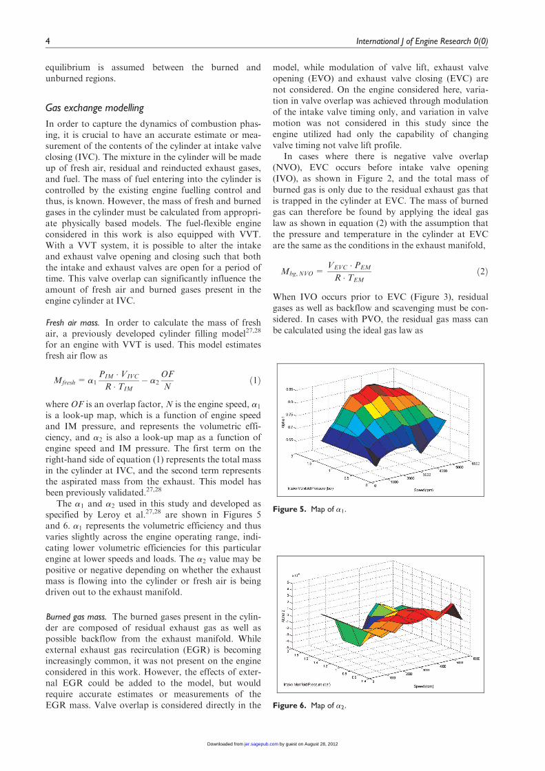
Fresh air mass. In order to calculate the mass of freshair, a previously developed cylinder filling model27,28
for an engine with VVT is used. This model estimatesfresh air flow as
Mfresh=a1PIM � VIVC
R � TIM� a2
OF
Nð1Þ
where OF is an overlap factor, N is the engine speed, a1
is a look-up map, which is a function of engine speedand IM pressure, and represents the volumetric effi-ciency, and a2 is also a look-up map as a function ofengine speed and IM pressure. The first term on theright-hand side of equation (1) represents the total massin the cylinder at IVC, and the second term representsthe aspirated mass from the exhaust. This model hasbeen previously validated.27,28
The a1 and a2 used in this study and developed asspecified by Leroy et al.27,28 are shown in Figures 5and 6. a1 represents the volumetric efficiency and thusvaries slightly across the engine operating range, indi-cating lower volumetric efficiencies for this particularengine at lower speeds and loads. The a2 value may bepositive or negative depending on whether the exhaustmass is flowing into the cylinder or fresh air is beingdriven out to the exhaust manifold.
Burned gas mass. The burned gases present in the cylin-der are composed of residual exhaust gas as well aspossible backflow from the exhaust manifold. Whileexternal exhaust gas recirculation (EGR) is becomingincreasingly common, it was not present on the engineconsidered in this work. However, the effects of exter-nal EGR could be added to the model, but wouldrequire accurate estimates or measurements of theEGR mass. Valve overlap is considered directly in the
model, while modulation of valve lift, exhaust valveopening (EVO) and exhaust valve closing (EVC) arenot considered. On the engine considered here, varia-tion in valve overlap was achieved through modulationof the intake valve timing only, and variation in valvemotion was not considered in this study since theengine utilized had only the capability of changingvalve timing not valve lift profile.
In cases where there is negative valve overlap(NVO), EVC occurs before intake valve opening(IVO), as shown in Figure 2, and the total mass ofburned gas is only due to the residual exhaust gas thatis trapped in the cylinder at EVC. The mass of burnedgas can therefore be found by applying the ideal gaslaw as shown in equation (2) with the assumption thatthe pressure and temperature in the cylinder at EVCare the same as the conditions in the exhaust manifold,
Mbg,NVO=VEVC � PEM
R � TEMð2Þ
When IVO occurs prior to EVC (Figure 3), residualgases as well as backflow and scavenging must be con-sidered. In cases with PVO, the residual gas mass canbe calculated using the ideal gas law as
Figure 5. Map of a1.
Figure 6. Map of a2.
4 International J of Engine Research 0(0)
by guest on August 28, 2012jer.sagepub.comDownloaded from

Mres =VIVO � PEM
R � TEMð3Þ
In the period of time between IVO and EVC, gasescan flow between the IM, the engine cylinder and theexhaust manifold (EM). Any residual exhaust gas thatis expelled into the IM will be reinducted during theintake stroke. In addition, depending on the placementof IVO and EVC and the pressure differential acrossthe engine, residual gas may flow into the exhaustmanifold or exhaust gas from the exhaust manifoldmay re-enter the cylinder (this is commonly referred toas backflow). The engine used in the study had an IVOand EVC that always occurred before TDC, and thusmass is always lost from the cylinder during valve over-lap. If IVO and EVC occurred after TDC, the pistonwould be moving downward during valve overlap, andexhaust gases could be reinducted back into the cylin-der. However, since valve overlap always occurs beforeTDC on this engine, the piston is moving upward, andvolume is being forced out of the cylinder during valveoverlap. The portion of residual gas that is lost to theintake and exhaust manifolds during this time of valveoverlap can be found using the ideal gas law. The frac-tion of this residual mass that exits the exhaust mani-fold is assumed to be proportional to the pressures inthe intake and exhaust manifolds. Thus, in a similarmethod as that used by Kocher et al.,29 these backfloweffects are captured by
Mbackflow=PIM
PIM +PEM� (VEVC � VIVO) � PEM
R � TEMð4Þ
Combining equations (3) and (4), the total burned gasmass in the case of valve overlap is
Mbg,PVO=VIVO � PEM
R � TEM
þ PIM
PIM +PEM� (VEVC � VIVO) � PEM
R � TEMð5Þ
Equations (1), (2), (5) and the controlled fuellingmass provide the composition of the cylinder mixtureat IVC. The BGF can then be computed by
Ybg=Mbg
Mbg+Mfreshð6Þ
where Mfresh is given by equation (1) and Mbg is givenby either equation (2) or (5), depending on the valveoverlap.
Compression modelling
After the contents of the cylinder (i.e. the burned gasmass and fresh air mass) are computed, the evolutionof the temperature and pressure of these contents fromIVC to SIT must be computed. In this phase, polytro-pic compression with a polytropic coefficient (n) of 1.29is assumed. Furthermore, the temperature and pressureat IVC are assumed to be approximately equal to those
in the IM. The conditions at SIT can be found by equa-tions (7) and (8).
PSIT =PIM �VIVC
VSIT
� �n
ð7Þ
TSIT =TIVC �VIVC
VSIT
� �n�1ð8Þ
The temperature at IVC, TIVC, is given by
TIVC=Ybg � TEM +(1� Ybg) � TIM ð9Þ
in order to take into account the effect of burned gaseson the initial temperature at IVC.
Flame-propagation modelling
Shortly after a spark is applied, the mixture will beginto burn. In order to estimate the time it takes for thefuel to burn, it is necessary to predict the manner inwhich the flame propagates.
Inputs. In addition to the pressure and temperature atSIT determined by equations (7) and (8) in the compres-sion phase of the model, it is also necessary to know themass fraction of fuel in the cylinder and the initial den-sity of the cylinder contents at SIT. Since the in-cylindercontents are assumed to be homogenous, the mass frac-tion of fuel in the unburned zone is
Yfuel, u =Mfuel
Mfuel +Mfresh +Mbgð10Þ
The initial density at SIT is
ru,SIT =Mfuel +Mfresh +Mbg
VSITð11Þ
Equations (7) to (11) provide the thermodynamic con-ditions at SIT and give the initial conditions for theflame-propagation model.
Mass fraction of fuel burned. Following SI, the rate atwhich fuel is burned can be described by
dmfuel
dt= ru �Uturb � A ð12Þ
where ru is the density in the unburned region, Uturb isthe turbulent flame speed, and A is the mean flame sur-face area.30 Note that since the mixture is assumed tobe homogenous, this rate of fuel burn will be the sameas the mixture burn rate.
Alternatively, the fraction of fuel burned (xfuel) iscaptured by the following relationship, which is derivedfrom equation (12),
dxfueldt
=1
MfuelYfuel, u � ru �Uturb � A ð13Þ
The total mass of fuel injected (Mfuel) is known andthe mass fraction of fuel (equation (10)) throughout theunburned zone is considered uniform due to the
Hall et al. 5
by guest on August 28, 2012jer.sagepub.comDownloaded from
homogeneity assumption. In order to evaluate equation(13), ru, Uturb and A must also be determined.
Unburned density and temperature. In order to calculatethe evolution of the temperature and density in theunburned zone, polytropic compression of theunburned gases is assumed,9,31,32 as captured by equa-tions (14) and (15),
Tu =Tu,SIT �P
PSIT
� �n�1n
ð14Þ
ru = ru,SIT �P
PSIT
� �1n
ð15Þ
The unburned density (ru) is required by equation(13), and the temperature in the unburned region willbe required for computation of the flame speed.
Heat transfer may affect this unburned temperatureand the impact of heat transfer is likely strongly depen-dent on the engine speed. However, this model uses theestimated unburned temperature solely in the calcula-tion of turbulent flame speed and the relationship forturbulent flame speed does include several tuning fac-tors that provide a dependence on engine speed. Thus,this effect of heat transfer on temperature and thereforeflame speed is most likely being captured by the tuningfor the turbulent flame speed model as detailed in thesection on turbulent flame speed.
In-cylinder pressure. The in-cylinder pressure and heat-release analysis is modelled based on first principles.While the approach is straightforward, it appears tocapture the burn rate accurately and similar physics-based methods have been extensively used in othercontrol-oriented models (such as those by Hillion etal.31,32 and Koeberlein33) with promising results.
The change in pressure in the flame-propagationstage can be deduced from the First Law ofThermodynamics
dE
dt=
dQ
dt� dW
dt+X
_mihi ð16Þ
which can be rewritten for a closed system as
dU
dt=
dQ
dt� P
dV
dtð17Þ
Assuming constant specific heats and an ideal gas,equation (17) becomes
(g � 1)dQ
dt= g � PdV
dt+V
dP
dtð18Þ
Furthermore, the heat addition due to combustion ofthe fuel can be expressed as
dQ
dt=Mfuel �QLHV �
dxfdt
ð19Þ
in which QLHV is the lower heating value of the fuelused.
Plugging equation (19) into equation (18) yields
(g � 1) �Mfuel �QLHV �dxfueldt
= g � PdV
dt+V
dP
dt
ð20Þ
which is used to evaluate the evolution of in-cylinderpressure following SIT.32
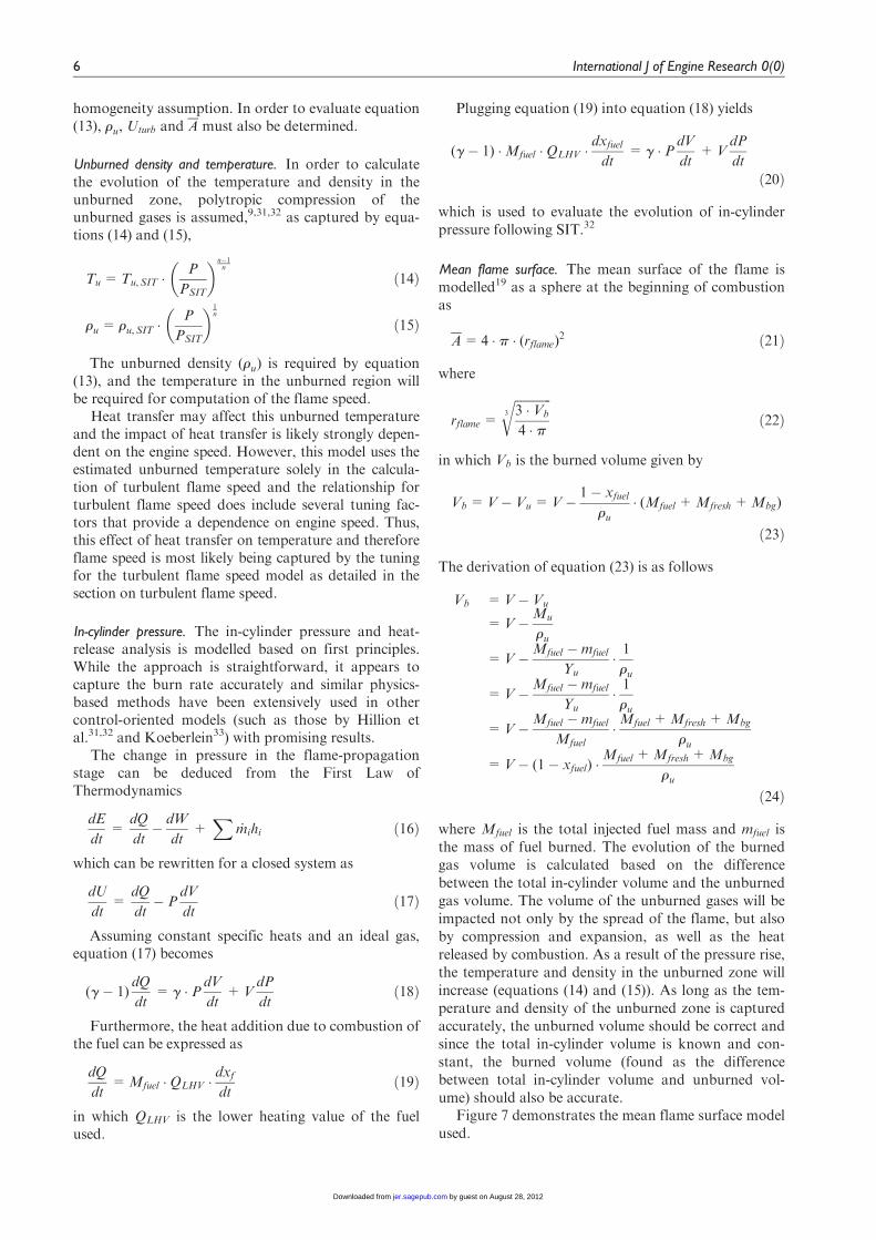
Mean flame surface. The mean surface of the flame ismodelled19 as a sphere at the beginning of combustionas
A=4 � p � (rflame)2 ð21Þ
where
rflame =
ffiffiffiffiffiffiffiffiffiffiffiffi3 � Vb
4 � p3
rð22Þ
in which Vb is the burned volume given by
Vb =V� Vu =V� 1� xfuelru
� (Mfuel +Mfresh+Mbg)
ð23Þ
The derivation of equation (23) is as follows
Vb =V� Vu
=V�Mu
ru
=V�Mfuel �mfuel
Yu� 1ru
=V�Mfuel �mfuel
Yu� 1ru
=V�Mfuel �mfuel
Mfuel�Mfuel +Mfresh+Mbg
ru
=V� (1� xfuel) �Mfuel +Mfresh +Mbg
ru
ð24Þ
where Mfuel is the total injected fuel mass and mfuel isthe mass of fuel burned. The evolution of the burnedgas volume is calculated based on the differencebetween the total in-cylinder volume and the unburnedgas volume. The volume of the unburned gases will beimpacted not only by the spread of the flame, but alsoby compression and expansion, as well as the heatreleased by combustion. As a result of the pressure rise,the temperature and density in the unburned zone willincrease (equations (14) and (15)). As long as the tem-perature and density of the unburned zone is capturedaccurately, the unburned volume should be correct andsince the total in-cylinder volume is known and con-stant, the burned volume (found as the differencebetween total in-cylinder volume and unburned vol-ume) should also be accurate.
Figure 7 demonstrates the mean flame surface modelused.
6 International J of Engine Research 0(0)
by guest on August 28, 2012jer.sagepub.comDownloaded from
After the flame reaches the piston head, the flameprogressively becomes a cylinder and the flame area iscalculated by equations
A=2 � p � (rflame) � dl ð25Þ
rflame =
ffiffiffiffiffiffiffiffiffiffiffiVb
p � dl
rð26Þ
The distance between the cylinder head and the pistonis dl.
Turbulent flame speed. The turbulent flame speed, Uturb,has been shown to be proportional to the intensity ofturbulence in-cylinder and the laminar flame speed. Anumber of factors including valve overlap and spark tim-ing, as well as in-cylinder swirl and tumble, can have animpact on the turbulence intensity. However, researchersat the University of Michigan34 have demonstrated thatthe main driver for in-cylinder turbulence is engine speedand that other factors had only minor effects. Therefore,in an effort to keep the model control amenable, turbu-lence intensity is modelled solely as a function of enginespeed. While a more complex model may improve per-formance slightly, there did not appear to be a significantdetrimental impact due to considering only the majordriver of turbulence (engine speed).
Thus, turbulent flame speed is expressed as
Uturb = f �UL ð27Þ
in which f is a turbulence-enhancement factor that isproportional to engine speed and UL is the laminarflame speed.34–36 The laminar flame speed is obtainedby
UL =UL, 0Tu
Tamb
� �aP
Pamb
� �b
(1� 2:06 � Y0:75bg ) ð28Þ
UL, 0 =Z �W � fh � e�j�(f�1:075)2 ð29Þ
in which Z is fuel dependent and W, h, j, a, and b arefuel independent. The mass fraction of burned gases isYbg. This relationship was developed by Bayraktar,37
Gulder,38 Metghalchi and Keck,39 Bonatesta andShayler,40 Syed et al.41 and Lindstrom et al.42 The val-ues for Z, W, h, j, a, and b are given in Table 2, inwhich VE is the volume fraction of ethanol in the fuel.These constants were tuned for this model but are inclose agreement with studies by Syed et al.,41
Bayraktar37 and Lindstrom et al.42 The linear depen-dance of laminar flame speed on ethanol blend is cap-tured by Z. While Gulder created a laminar flamespeed correlation for ethanol blends43 that has beenused extensively, more recent studies (which havefocused on a broader range of ethanol blends, pressuresand temperatures) have shown more linear increases inflame speed with respect to ethanol content.41,44,45 Inagreement with the studies of Syed et al.,41 Broustailet al.44 and Hara and Tanoue,45 as well as the trendsobserved in this study, a linear correlation for Z wasused that corresponds to a 10% increase in laminarflame speed at E100.
The turbulent flame speed is then calculated by
Uturb =(a �N+ b) �UL, 0Tu
Tamb
� �aP
Pamb
� �b
1� 2:06 � Y0:75bg
� �ð30Þ
where a and b are constants of 0.0025 and 3.4,respectively.
Model summary
This flame-propagation model is physically based andgeneralizable to different engine architectures. It alsotakes into account the ethanol blend ratio and in-cylinder burned gas. The complexity of the model iskept to a minimum in order to allow the model to beused for control purposes. The entire flame-propagation model is captured by the following two-state model, in which the states are the fraction of fuelburned (xfuel) and the in-cylinder pressure. The firststate equation is obtained by substituting equationsobtained by combining equations (10), (11), (14), (15)and (30) into equation (13), yielding
dxfueldt = 1
VSIT� Tu,SIT
Tamb
� �a
� P(1+ (n�1)�a)=n+b
P(1+ (n�1)�a)=nSIT
�Pb
amb
� �
�(a �N+ b) �UL, 0 � 1� 2:06 � Y0:75bg
� �� A ð31Þ
Figure 7. Mean flame surface area model.
Table 2. Values for constants in laminar flame speed.
Z 1 � (1� VE) + 1:1 � VE
W 0.4658h 0.3j 4.48a 0.9b 20.05
Hall et al. 7
by guest on August 28, 2012jer.sagepub.comDownloaded from
in which temperature and pressure at SIT can be deter-mined by equations (7) to (9) and values for UL, 0 andYbg are given by equations (29) and (6), respectively.
The second state equation is found by rearrangingequation (18) to solve for the rate of change in pressureas captured by equation (32).
dP
dt=
g � 1
V�Mfuel �QLHV �
dxfueldt� g � PdV
dtð32Þ
Model validation
The previous section outlined all of the equations neces-sary to describe the gas exchange, compression andflame-propagation models, as illustrated in Figure 4.Experimentation to validate the model was conductedon a Renault F4RT 2.1 l engine with VVT on the intakevalves. Variation in valve overlap on this engine wasachieved through modulation of the intake valve timingonly. The engine is port-fuel injected and turbocharged.The specifications for this engine are given in Table 3.
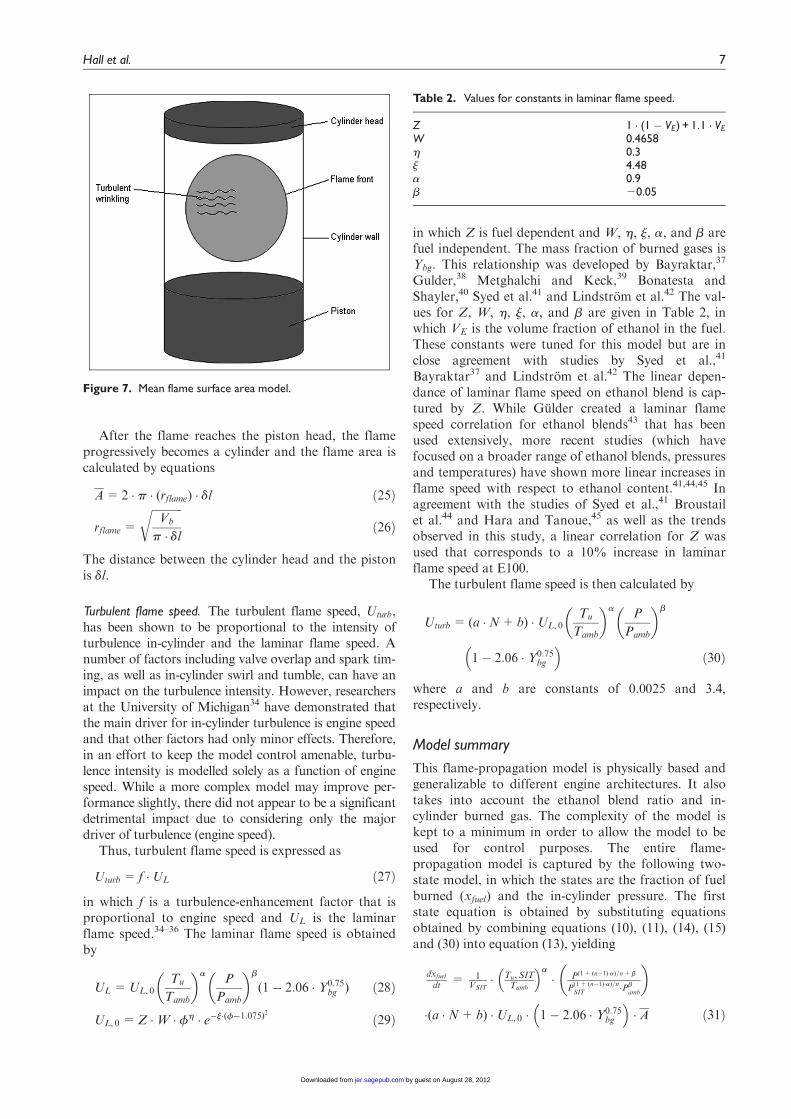
The model was validated at over 500 operatingpoints consisting of varying combinations of speed, IMpressure, valve overlap, SIT and ethanol blend fraction.In this study, valve overlap was accomplished by alter-ing the intake timing, as shown in Figures 2 and 3. Thefuels considered in the study include E0 (gasoline), E5(5% ethanol / 95% gasoline), E40 (40% ethanol / 60%gasoline), and E85 (85% ethanol / 15% gasoline).Engine speed, IM pressure, valve overlap and SIT werevaried over the ranges shown in Table 4.
As shown in Figure 8, the operating points at whichthe model was validated cover a variety of speed/loadconditions with all four fuel blends.
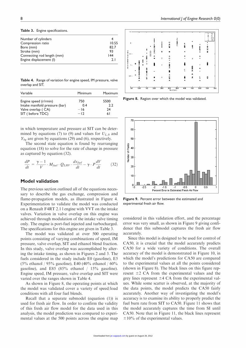
Recall that a separate submodel (equation (1)) isused for fresh air flow. In order to confirm the validityof this fresh air flow model for the data used in thisanalysis, the model prediction was compared to experi-mental values at the 500 points across the engine map
considered in this validation effort, and the percentageerror was very small, as shown in Figure 9 giving confi-dence that this submodel captures the fresh air flowaccurately.
Since this model is designed to be used for control ofCA50, it is crucial that the model accurately predictsCA50 for a wide variety of conditions. The overallaccuracy of the model is demonstrated in Figure 10, inwhich the model’s predictions for CA50 are comparedto the experimental values at all the points considered(shown in Figure 8). The black lines on this figure rep-resent 62 CA from the experimental values and thegrey lines represent 64 CA from the experimental val-ues. While some scatter is observed, at the majority ofthe data points, the model predicts the CA50 fairlyaccurately. Another way of investigating the model’saccuracy is to examine its ability to properly predict thefuel burn rate from SIT to CA50. Figure 11 shows thatthe model accurately captures the time from SI untilCA50. Note that in Figure 11, the black lines represent610% of the experimental values.
Table 3. Engine specifications.
Number of cylinders 4Compression ratio 10.55Bore (mm) 82.7Stroke (mm) 93Connecting rod length (mm) 144Engine displacement (l) 2.1
Table 4. Range of variation for engine speed, IM pressure, valveoverlap and SIT.
Variable Minimum Maximum
Engine speed (r/rmin) 750 5500Intake manifold pressure (bar) 0.4 2.2Valve overlap ( CA) 216 24SIT ( before TDC) 212 61
Figure 8. Region over which the model was validated.
Figure 9. Percent error between the estimated andexperimental fresh air flow.
8 International J of Engine Research 0(0)
by guest on August 28, 2012jer.sagepub.comDownloaded from
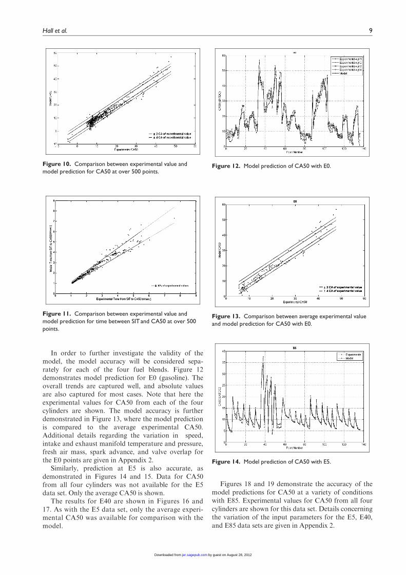
In order to further investigate the validity of themodel, the model accuracy will be considered sepa-rately for each of the four fuel blends. Figure 12demonstrates model prediction for E0 (gasoline). Theoverall trends are captured well, and absolute valuesare also captured for most cases. Note that here theexperimental values for CA50 from each of the fourcylinders are shown. The model accuracy is furtherdemonstrated in Figure 13, where the model predictionis compared to the average experimental CA50.Additional details regarding the variation in speed,intake and exhaust manifold temperature and pressure,fresh air mass, spark advance, and valve overlap forthe E0 points are given in Appendix 2.
Similarly, prediction at E5 is also accurate, asdemonstrated in Figures 14 and 15. Data for CA50from all four cylinders was not available for the E5data set. Only the average CA50 is shown.
The results for E40 are shown in Figures 16 and17. As with the E5 data set, only the average experi-mental CA50 was available for comparison with themodel.
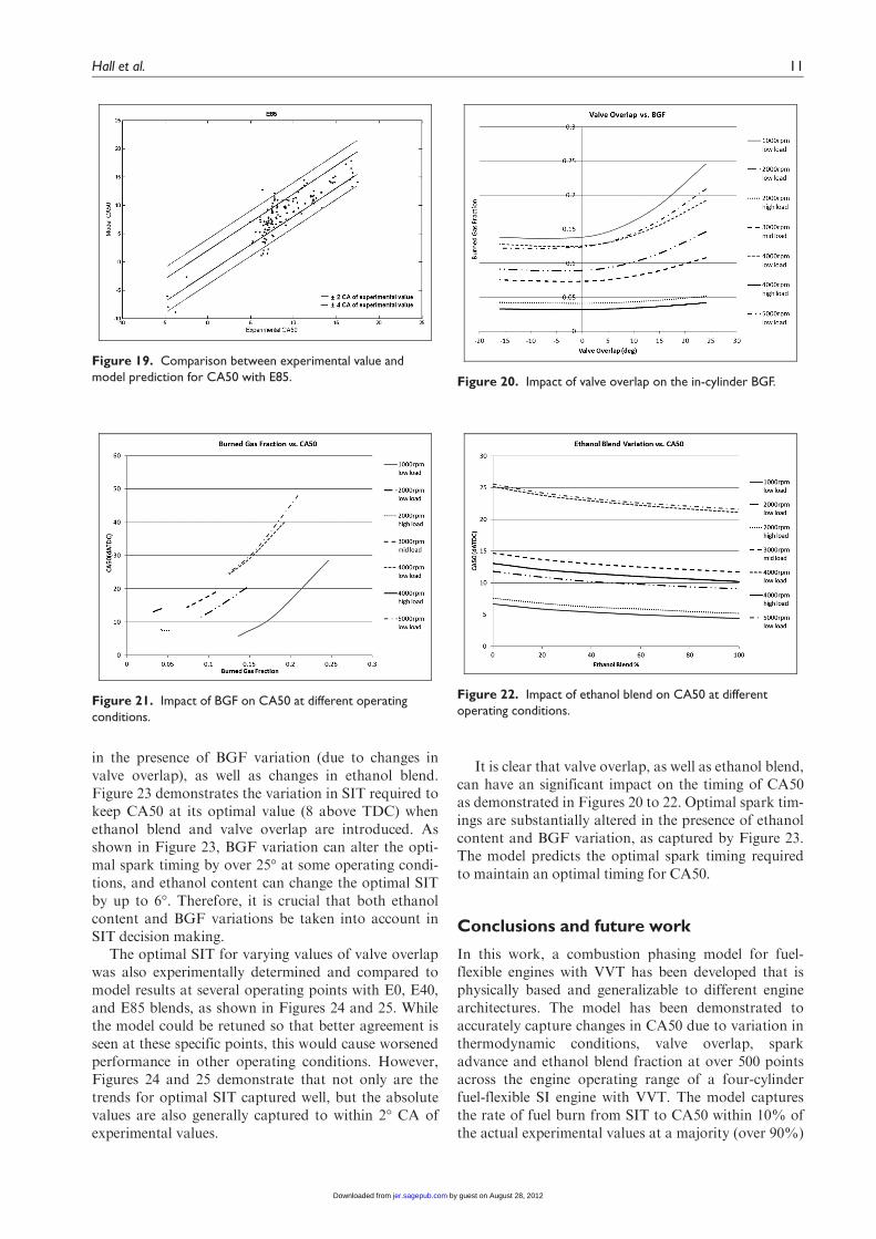
Figures 18 and 19 demonstrate the accuracy of themodel predictions for CA50 at a variety of conditionswith E85. Experimental values for CA50 from all fourcylinders are shown for this data set. Details concerningthe variation of the input parameters for the E5, E40,and E85 data sets are given in Appendix 2.
Figure 10. Comparison between experimental value andmodel prediction for CA50 at over 500 points.
Figure 11. Comparison between experimental value andmodel prediction for time between SIT and CA50 at over 500points.
Figure 12. Model prediction of CA50 with E0.
Figure 13. Comparison between average experimental valueand model prediction for CA50 with E0.
Figure 14. Model prediction of CA50 with E5.
Hall et al. 9
by guest on August 28, 2012jer.sagepub.comDownloaded from

In summary and as demonstrated in Figures 10 and11, the model is quite accurate for the vast majority ofthe operating conditions, BGFs and ethanol blendsconsidered.
Sensitivity of CA50 to inputs
As demonstrated in the previous section, this physicallybased, generalizable model accurately predicts CA50under a variety of different operating conditions.Therefore, the model can be used to investigate theinfluence of different inputs on the CA50 timing. Valveoverlap and SIT are control inputs that affect the gasexchange and flame-propagation processes, while etha-nol blend ratio can be considered a disturbance (uncon-trolled input) to the system. In this section, the modelwill be utilized to study the influence of valve overlap,ethanol blend and spark timing on CA50.
Valve overlap affects the amount of burned gasespresent in the cylinder, as demonstrated in Figure 20for E0. In regions of NVO, the effect of valve overlapon the BGF is negligible; however, when PVO isachieved, the BGF increases as PVO increases. This
effect is different depending on the operating condi-tions. At some operating points, the intake and exhaustmanifolds have similar pressures and the BGF is rela-tively constant, regardless of valve overlap. However,at other operating points, there is a larger pressure dif-ference across the engine and the resulting BGFs canbe significant (up to 25%), as shown in Figure 20.
Since valve overlap affects the BGF, it also influencesthe CA50 (equation (28)). As shown in Figure 21, CA50increases as BGF increases due to the impact of BGFon flame speed, as captured by equation (30).
As described previously, increasing the ethanolblend fraction decreases CA50 due to the faster flamespeeds of ethanol.37,44,43,41 Since the equivalence ratiois kept at 1, increasing the ethanol blend also requiresan increase in fuelling (due to the lower stoichiometricAFR of ethanol). Figure 22 demonstrates the impact ofhigher flame speeds (via equation (29)) on CA50 reduc-tion. A change in ethanol blend from E0 to E85 cancause up to a 6� change in CA50.
The spark timing also directly affects the CA50 tim-ing, since it dictates the start of the flame-propagationprocess. Earlier spark timings lead to earlier CA50s.Spark timing can be used to maintain an optimal CA50
Figure 15. Comparison between average experimental valueand model prediction for CA50 with E5.
Figure 16. Model prediction of CA50 with E40.
Figure 17. Comparison between average experimental valueand model prediction for CA50 with E40.
Figure 18. Model prediction of CA50 with E85.
10 International J of Engine Research 0(0)
by guest on August 28, 2012jer.sagepub.comDownloaded from
in the presence of BGF variation (due to changes invalve overlap), as well as changes in ethanol blend.Figure 23 demonstrates the variation in SIT required tokeep CA50 at its optimal value (8 above TDC) whenethanol blend and valve overlap are introduced. Asshown in Figure 23, BGF variation can alter the opti-mal spark timing by over 25� at some operating condi-tions, and ethanol content can change the optimal SITby up to 6�. Therefore, it is crucial that both ethanolcontent and BGF variations be taken into account inSIT decision making.
The optimal SIT for varying values of valve overlapwas also experimentally determined and compared tomodel results at several operating points with E0, E40,and E85 blends, as shown in Figures 24 and 25. Whilethe model could be retuned so that better agreement isseen at these specific points, this would cause worsenedperformance in other operating conditions. However,Figures 24 and 25 demonstrate that not only are thetrends for optimal SIT captured well, but the absolutevalues are also generally captured to within 2� CA ofexperimental values.
It is clear that valve overlap, as well as ethanol blend,can have an significant impact on the timing of CA50as demonstrated in Figures 20 to 22. Optimal spark tim-ings are substantially altered in the presence of ethanolcontent and BGF variation, as captured by Figure 23.The model predicts the optimal spark timing requiredto maintain an optimal timing for CA50.
Conclusions and future work
In this work, a combustion phasing model for fuel-flexible engines with VVT has been developed that isphysically based and generalizable to different enginearchitectures. The model has been demonstrated toaccurately capture changes in CA50 due to variation inthermodynamic conditions, valve overlap, sparkadvance and ethanol blend fraction at over 500 pointsacross the engine operating range of a four-cylinderfuel-flexible SI engine with VVT. The model capturesthe rate of fuel burn from SIT to CA50 within 10% ofthe actual experimental values at a majority (over 90%)
Figure 19. Comparison between experimental value andmodel prediction for CA50 with E85. Figure 20. Impact of valve overlap on the in-cylinder BGF.
Figure 21. Impact of BGF on CA50 at different operatingconditions.
Figure 22. Impact of ethanol blend on CA50 at differentoperating conditions.
Hall et al. 11
by guest on August 28, 2012jer.sagepub.comDownloaded from

of these points. Furthermore, its computational simpli-city and the fact that it uses only available engine
sensor measurements make it extremely valuable forefforts to control combustion phasing.
In current control methods, static look-up tables areused extensively for control of ignition, and while suchtables provide acceptable control in steady state fortheir intended fuel, significant performance is lostduring transients and when other alternative fuels areutilized. Since the model detailed in this paper canpredict CA50 on a cycle-to-cycle basis for multiplefuels, it can be used to correct or replace the existinglook-up tables. This could be done by comparing theestimated CA50 given by the model to a desired CA50(which is typically known for an engine). The errorbetween the desired and estimated CA50 can be usedto drive feedback and feedforward control algorithms,which would adjust the spark advance timing to anoptimal timing that provides the desired combustionphasing. Future efforts will focus on developing suchcontrol strategies in order to improve performanceduring transients and when operating with alternativefuels and VVT.
Funding
This work was supported by the National ScienceFoundation Graduate Research Fellowship [grant no.103049 – award no. 0833366].
Acknowledgements
Special thanks to IFP Energies Nouvelles for providingexperimental support on this project. The authors alsowish to thank Lyle Kocher, Gayatri Adi, ThomasLeroy, and Thomas Coppin for their advice and contri-butions to this work.
References
1. Coppin T, Grondin O, Maamri N, and Rambault L.
Fuel estimation and air-to-fuel ratio control for flexfuel
spark-ignition engines. In: 2010 IEEE International Con-
ference on Control Applications, 2010.2. Nakata K, Utsumi S, Ota A, Kawatake K, Kawai T,
and Tsunooka T. The effect of ethanol fuel on a spark
ignition engine. SAE paper 2006-01-3380, 2006.3. Caton PA, Hamilton LJ, and Cowart JS. An experimen-
tal and modeling investigation into the comparative
knock and performance characteristics of e85, gaso-
hol[e10] and regular unleaded gasoline[87(r+m)/2]. SAE
paper 2007-01-0473, 2007.4. Cairns A, Todd A, ALeiferis P, Fraser N, and Malcolm
J. A study of alcohol blended fuels in an unthrottled sin-
gle cylinder spark ignition engine. SAE paper 2010-01-
0618, 2010.5. Coppin T, Grondin O, Le Solliec F, Rambault, and N.
Maamri L. Control-oriented mean-value model of a fuel-
flexible turbocharged spark-ignition engine. SAE paper
2010-01-0937, 2010.6. Ahn K, Stefanopoulou A, and Jankovic M. Estimation
of ethanol content in flex-fuel vehicles using an exhaust
gas oxygen sensor: Model, tuning, and sensitivity. In:
Figure 23. SIT required to obtain the optimal CA50 atdifferent operating conditions.
Figure 24. SIT required to obtain the optimal CA50 atdifferent operating conditions.
Figure 25. SIT required to obtain the optimal CA50 atdifferent operating conditions.
12 International J of Engine Research 0(0)
by guest on August 28, 2012jer.sagepub.comDownloaded from

2008 Proceedings of the ASME Dynamic Systems and
Control Conference, pages 1309–1316, 2008.7. Ahn K, Stefanopoulou A, and Jankovic M. Tolerant
ethanol estimation in flex-fuel vehicles during MAF sen-
sor drifts. In: Proceedings of the ASME 2009 Dynamic
Systems and Control Conference, 2009.8. Ahn K, Stefanopoulou A, and Jankovic M. Fuel puddle
model and afr compensator for gasoline-ethanol blends
in flex-fuel engines. In: Proceedings of the IEEE Vehicle
Power and Propulsion Conference, 2009.9. Heywood J. Internal combustion engine fundamentals.
New York: McGraw-Hill, 1988.10. Nakama K, Kusaka J, and Daisho Y. Effect of ethanol
on knock in spark ignition gasoline engines. SAE paper
2008-32-0020, 2008.11. Fontana G, Galloni E, Palmaccio R, and Torella E. The
influence of variable valve timing on the combustion pro-
cess of a small spark-ignited engine. SAE paper 2006-01-
0445, 2006.12. Cairns A, Todd A, Hoffman H, ALeiferis P, and Mal-
colm J. Combining unthrottled operation with internal
EGR under port and central direct fuel injection condi-
tions in a single cylinder SI engine. SAE paper 2009-01-
1835, 2009.
13. Sher E and Bar-Kohany T. Optimization of variable
valve timing for maximizing performance of an
unthrottled SI engine – a theoretical study. Energy,
27:757–775, 2002.14. Scharrer O, Heinrich C, Heinrich M, Gebhard P, and
Pucher H. Review and analysis of variable valve timing
strategies - eight ways to approach. SAE paper 2004-01-
0614, 2004.15. Hong H, Parvate-Patil GB, and Gordon B. Review and
analysis of variable valve timing strategies - eight ways to
approach. Proc IMechE, Part D: J Automobile Engineer-
ing 2004; 218: 1179–1200.16. Cleary D and Silvas G. Unthrottled engine operation
with variable intake valve lift, duration, and timing. SAE
paper 2007-01-1282, 2007.17. Song J and Sunwoo M. Flame kernal formation and pro-
pagation modelling in spark ignition engines. Proc
IMechE, Part D: J Automobile Engineering 2001; 218:
105–114.18. Bade Shrestha SO and Karim GA. A predictive model for
gas fueled spark ignition engine applications. SAE paper
1999-01-3482, 1999.19. Lafossas FA, Colin O, Le Berr F, and Menegassi P.
Application of a new 1D combusiton model to gasoline
transient engine operation. SAE paper 2005-01-2107,
2005.20. Bougrine A, Richard S, and Veynante D. Modelling and
simulation of the combustion of ethanol blended fuels in
a SI engine using a 0D coherent flame model. SAE paper
2009-24-0016, 2009.21. Richard S, Bougrine S, Font G, Lafossas FA, and Le
Berr F. On the reduction of a 3D CFD combustion model
to build a physical 0D model for simulating heat release,
knock and pollutants in SI engines. Oil Gas Sci Tech –
Rev. IFP, 64(3):223–242, 2009.22. Le Berr F, Miche M, Le Solliec G, Lafossas FA, and
Colin G. Modelling of a turbocharged SI engine with
variable camshaft timing for engine control purposes.
SAE paper 2006-01-3264, 2006.
23. Lee T-K, Kramer D, and Filipi Z. High-degree-of-free-
dom engine modelling for control design using a crank-
angle-resolved flame propagation simulation and artificial
neural network surrogate models. J Syst Contr Eng 2010;
224: 747–761.24. Ahn K, Stefanopoulou AG, Jiang L, and Yilmaz H.
Ethanol content estimation in flex fuel direct injection
engines using in-cylinder pressure measurements. In:
SAE World Congress, 2010.25. Oliverio N, Stefanopoulou A, Jiang L, and Yilmaz H.
Ethanol detection in flex-fuel direct injection engines
using in-cylinder pressure measurements. SAE paper
2009-01-0657, 2009.26. Theunissen FM. Percent ethanol estimation on sensorless
multi-fuel systems: advantages and limitations. SAE
paper 2003-01-3562, 2003.27. Leroy T, Alix G, Chauvin J, Duparchy A, and Le Berr
F. Modeling fresh air charge and residual gas fraction on
a dual independent variable valve timing SI engine. SAE
paper 2008-01-0983, 2008.28. Leroy T. Cylinder filling control of variable-valve-actuation
equipped internal combustion engines. PhD thesis, MINES
Paris Tech, 2010.29. Kocher L, Koeberlein E, Van Alstine D, Stricker K, and
Shaver G. Physically-based volumetric efficiency model
for diesel engines utilizing variable intake valve actuation.
In: 2011 Dynamics Systems and Control Conference, 2011.
30. Turns S. An introduction to combustion. New York:
McGraw-Hill, 2000.31. Hillion M, Chauvin J, and Petit N. Open-loop combus-
tion timing control of a spark-ignited engine. In: Proceed-
ings of the 47th IEEE Conference on Decision and Control,
2008.32. Hillion M. Transient combustion control of internal com-
bustion engines. PhD thesis, MINES Paris Tech, 2009.33. Koeberlein E, Kocher L, Van Alstine D, Stricker K, and
Shaver GM. Physics-based control-oriented modeling of
exhaust gas enthalpy for engines utilizing variable valve
actuation. In: 2011 Dynamic Systems and Control Confer-
ence Proceedings, 2011.34. Prucka R, Lee T, Filipi Z, and Assanis D. Turbulence
intensity calculation from cylinder pressure data in a high
degree of freedom spark-ignition engine. SAE paper
2010-01-0175, 2010.35. Hiroyasu H and Kadota T. Computer simulation for
combustion and exhaust emisssions on spark-ignition
engine. In: 15th Symposium (International) on Combus-
tion, pages 1213–1233, 1975.36. Ramos J. Internal combustion engine modeling. New
York: Hemisphere Publishing Corporation, 1989.37. Bayraktar H. Experimental and theoretical investigation
of using gasoline-ethanol blends in spark-ignition engines.
Ren Energy, 30:1733–1747, 2005.38. Gulder O. Laminar burning velocities of methanol, etha-
nol, isooctane-air mixtures. In: 19th Symposium (Interna-
tional) on Combustion, pages 275–281, 1982.39. Metghalchi M and Keck J. Burning velocities of mixtures
of air with methanol, isooctane and indolene at high pres-
sure and temperature. Comb Flame, 48:191–210, 1982.40. Bonatesta F and Shayler P. Factors influencing the burn
rate characteristics of a spark ignition engine with vari-
able valve timing. Proc IMechE, Part D: J Automotobile
Engineering, 222(11):2147–2158, 2008.
Hall et al. 13
by guest on August 28, 2012jer.sagepub.comDownloaded from
41. Syed I, Yeliana, Mukherjee A, Naber J, and Michalek D.Numerical investigation of laminar flame speed of gaso-line-ethanol/air mixtures with varying pressure, tempera-ture, and dilution. SAE paper 2010-01-0620, 2010.
42. Lindstrom F, Angstrom H, Kalghatgi G, and Moller C.An emperical SI combustion model using laminar burn-ing velocity correlations. SAE paper 2005-01-2106,2005.
43. Gulder OL. Correlations of laminar combustion datafor alternative s.i. engine fuels. SAE paper 8410000,1984.
44. Broustail G, Seers P, Halter F, Moreac G, and Mou-naim-Rousselle C. Experimental determination of lami-nar burning velocity for butanol and ethanol iso-octaneblends. Fuel, 90:1–6, 2011.
45. Hara T and Tanoue K. Laminar flame speed of ethanol,n-heptane, iso-octane air mixtures. JSAE paper
20068518, 2006.
Appendix 1
Notation�A mean flame areaamb ambientb burnedbg burned gasE energyf turbulence-enhancement factorh enthalpymfuel mass of fuel burnedM massMfresh fresh air massMfuel injected fuel massn polytropic coefficientN engine speedP pressureQ heatQLHV lower heating valueres residualrflame flame radiusR universal gas constantT temperatureu unburnedU internal energyUL laminar flame speedUturb turbulent flame speedV volumeW workxfuel mass fraction of burned fuelYbg burned gas fractionYfuel, u mass fraction of fuel in the unburned
zoneg ratio of the heat capacity at constrant
pressure to heat capacity at constantvolume
dI distance between cylinder head andpiston
f equivlance ratioru density in the unburned zone
Applitions
AFR air-fuel ratioBGF burned gas fractionCA crank angleCA50 CA when 50% of the fuel has burnedE0 gasolineE5 5% ethanol/95% gasolineE40 40% ethanol/60% gasolineE85 85% ethanol/15% gasolineEGR exhaust gas recirculationEM exhaust manifoldEVC exhaust valve closingEVO exhaust valve openingIM intake manifoldIVC intake valve closingIVO intake valve openingNVO negative valve overlapOF overlap factor,PVO positive valve overlapSI spark ignitionSIT SI timingTDC top dead centerVVT variable valve timing
Appendix 2
Summary of model input variation
Figure 26 shows the variation in speed, intake andexhaust manifold temperature and pressure, fresh airmass, spark advance, and valve overlap at the E0 points.These are the inputs to the engine cylinder that affect thegas exchange and compression processes, as shown inFigure 4. The engine speed affects the amount of turbu-lence in-cylinder (equation (30)). The intake and exhaustpressures will affect the gas exchange process by directlyimpacting the mass of fresh (equation (1)) and burnedgases (equations (2) and (5)). Higher intake pressures areindicative of higher load conditions on the engine (whichrequire higher air and fuel flows). While the intake tem-peratures are approximately constant, the exhaust tem-perature varies more substantially depending on theengine load. These exhaust temperature changes impactthe burned gas mass (equations (2) and (5)), as well asthe temperature at IVC (equation (9)). The fresh air massis typically higher for higher loads and both the trendsand absolute values are captured well by the fresh airsubmodel (equation (1)). Spark timing is also signifi-cantly varied and directly impacts a number of inputs tothe flame-propagation model. Valve overlap also affectsthe mass of burned gases. As valve overlap increases andBGF increases, flame speeds are slowed and earlier sparktiming is required to maintain the same CA50. Thesecylinder inputs are used in the gas exchange and com-pression models. Following these phases, the initial con-ditions to the flame-propagation model (Figure 4) arecalculated to be those shown in Figure 27. The fuel massfraction, in-cylinder pressure, temperature, volume, den-sity, BGF and equivalence ratio all impact the speed at
14 International J of Engine Research 0(0)
by guest on August 28, 2012jer.sagepub.comDownloaded from
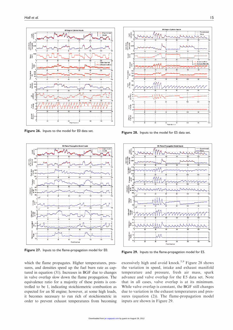
which the flame propagates. Higher temperatures, pres-sures, and densities speed up the fuel burn rate as cap-tured in equation (31). Increases in BGF due to changesin valve overlap slow down the flame propagation. Theequivalence ratio for a majority of these points is con-trolled to be 1, indicating stoichiometric combustion asexpected for an SI engine; however, at some high loads,it becomes necessary to run rich of stoichiometric inorder to prevent exhaust temperatures from becoming
excessively high and avoid knock.5,9 Figure 28 showsthe variation in speed, intake and exhaust manifoldtemperature and pressure, fresh air mass, sparkadvance and valve overlap for the E5 data set. Notethat in all cases, valve overlap is at its minimum.While valve overlap is constant, the BGF still changesdue to variation in the exhaust temperatures and pres-sures (equation (2)). The flame-propagation modelinputs are shown in Figure 29.
Figure 26. Inputs to the model for E0 data set.
Figure 27. Inputs to the flame-propagation model for E0.
Figure 28. Inputs to the model for E5 data set.
Figure 29. Inputs to the flame-propagation model for E5.
Hall et al. 15
by guest on August 28, 2012jer.sagepub.comDownloaded from
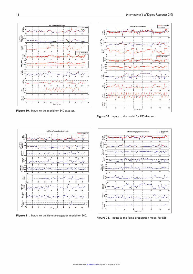
Figure 30. Inputs to the model for E40 data set.
Figure 31. Inputs to the flame-propagation model for E40.
Figure 32. Inputs to the model for E85 data set.
Figure 33. Inputs to the flame-propagation model for E85.
16 International J of Engine Research 0(0)
by guest on August 28, 2012jer.sagepub.comDownloaded from