Jed Singer and Gabriel Kreiman Summary - Harvard...

Q

Kriegeskorte—Transformations of Lamarckism

Introduction to Statistical Learning and Pattern Classification

Jed Singer and Gabriel Kreiman

Summary

Many of the chapters here concerned with experimental work (both for neurophysi-ological recordings and functional imaging measurements) have taken advantage of powerful machine learning techniques developed in the last several decades. Here we describe the underlying mathematics, discuss issues that are relevant to those who study the brain, and summarize current applications of these techniques. Chap-ters 19 and 20 extend these concepts and are concerned with the application of such techniques to neuronal and fMRI data, respectively. The material presented here is only an introduction to the topic, and the reader desiring more thorough coverage should consult more advanced textbooks (e.g., Bishop, 1995; Cristianini and Shawe-Taylor, 2000; Duda and Hart, 1973; Gabbiani and Cox 2010; Hertz et al 1992; Poggio and Smale 2003; Poggio et al 2004; Vapnik, 1995). Press et al. (1996) is also an excellent reference for computational algorithms to efficiently implement these techniques.

How Does a Machine Learn?

Let xi be a point in �d (that is, a vector with d dimensions). The data could corre-spond to the number of spikes fired by a single neuron in each of d different time windows, spike counts from d neurons during one time interval, features extracted from field potential recordings by d electrodes, or any other source of interest. Chapter 19 discusses in further detail the extraction of relevant features from neuro physiological recordings to use as input to a statistical classifier. We assume here that there are N such data, so that i ranges from 1 to N. In the context of a neuro-physiological experiment, N could correspond to the number of repetitions of a recording made under particular conditions. Each xi is associated with a label yi that describes it in some way. For example, yi could represent the identity or the category of the stimulus. The goal of machine learning is to establish a relationship

18

8404_018.indd 497 5/27/2011 7:41:01 PM

gabrielkreiman

Cross-Out

Q


498 Jed Singer and Gabriel Kreiman

between data and their labels; this relationship can then be used to predict the labels for new data (and can also tell us something about the properties of the data). The process by which such a relationship is discovered or approximated is called learn-ing. Labels can be as simple as values that are either 1 or –1, in the case of a binary classifier, or they may be of higher dimension and/or continuous-valued (in the continuous case the machine learning task is referred to as regression).

When we know the labels associated with data, that is we know ( , )xi iy , we can use this knowledge to guide the discovery of the relationship between x and y. This is called supervised learning. For example, if we have recorded spike counts over some window after presentation of a visual stimulus, we know both the data (spike counts) and the labels (the visual stimulus) for each trial. We could then relate the two using a supervised learning technique and use the discovered relationship to “read out” the stimulus in a new trial and to help explain the neural code for visual stimuli.

Sometimes, however, we do not know the labels. Say we have only a log of scalp electroencephalographic (EEG) signals recorded through a night’s sleep—we have the data, but we do not know any labels to which to relate them. There are unsu-pervised learning techniques that will operate upon a collection of unlabeled data and attempt to find structure within it. It is then up to the investigator to assign meaning to this structure.

It is not always clear what the data, the collection of xi values, should be. Differ-ent experimental techniques, from single-unit recordings to fMRI, yield data at different temporal and spatial scales and resolutions, often of very high dimensional-ity. The choice of how to process these data and which features to use can have a dramatic impact on the outcome or even the feasibility (see the “Curse of Dimen-sionality” section) of a learning algorithm. These decisions, and techniques to aid in making them, are discussed in chapter 19. It is important to note that, because the choice of features can have a profound impact on the results of the learning algo-rithm, those results must be understood in context. High classification performance indicates that the chosen features carry information about the labels assigned to their values. Low classification performance, however, indicates only that the learn-ing technique used was unable to discover a relationship between the chosen fea-tures and the labels. Different features may yield higher performance, as may a different learning algorithm. It is dangerous to compare high and low performance computed using different features and labels and conclude that more information about the labels is present in the data from the first set of features than from the second.

The nature of the labels, the yi values, is generally well specified in the case of supervised learning. These are the observed or experimentally controlled variables that are to be related to the physiological data. There is some freedom to choose

8404_018.indd 498 5/27/2011 7:41:01 PM

Q


Introduction to Statistical Learning and Pattern Classification 499

the details of representation; this goes hand in hand with choosing a learning algo-rithm and often reflects what one is trying to learn about the data. For example, real-valued labels are necessary for regression, in which one directly relates varia-tion in neural data to variation on some observed or controlled axis. Categorical data lend themselves to a classification algorithm, in which the neural data are segregated into labeled compartments. Continuous values can be compartmental-ized, if one wishes to use a classification algorithm—for example, into “low,” “medium,” and “high” values.

The use of machine-learning approaches is certainly not restricted to neuro science applications. These types of algorithms have emerged from applied mathe-matics and computer science investigations and find extensive applications in a variety of domains from weather prediction to computer vision, financial predic-tions, and many more.

The “Curse of Dimensionality,” Dimensionality Reduction, and Unsupervised Learning

Sampling in High-Dimensional Spaces

The machine learning techniques we discuss in this chapter use finite datasets to estimate properties about underlying, unknown distributions. To be able to do this successfully, however, requires that the available data sample the space in which they reside sufficiently densely. As the dimensionality of a space increases linearly, the number of points required to sample it at a given density increases exponentially. For example, a linear interval divided into two segments can be sampled at a density of one point per segment using only two points. A square with each dimension likewise divided requires four points, a cube eight, and so on. As the number of dimensions grows above a few, the number of points required for even this minimal coverage of the space quickly grows intractable. For this reason, choosing a repre-sentation for the data that minimizes its dimensionality while still preserving as much information as possible can dramatically improve the performance of machine learning techniques (which are themselves a form of dimensionality reduction).

Dimensionality Reduction

An important part of dimensionality reduction may come from knowledge about the problem at hand. For example, in the case of neurophysiological recordings, we generally have some a priori intuition about what the important aspects of the data “should” be, and we can take advantage of this knowledge. While the dimensionality of the space occupied by the data may be very high, we can often reduce it dramati-cally using heuristics. For example, rather than using the extracellular voltage

8404_018.indd 499 5/27/2011 7:41:01 PM

Q



recorded at 30 kHz resolution, most investigators high-pass filter and threshold the signal to end up with a binary representation of action potentials, sampled at a reso-lution of perhaps 1 kHz. In many cases, investigators further reduce the dimension-ality of the input by counting spikes in bins of a certain size. Care should always be taken in using such heuristics given that important aspects of the data may be dis-carded. In chapter 2, Nirenberg further discusses the relationship between spike counts and spike times. In chapter 21, Panzeri and Ince describe a systematic approach to study neural codes. Further discussion about feature extraction and formatting neuronal data are presented in chapter 19.

Several mathematical techniques are available for dimensionality reduction (Bishop, 1995; Gabbiani and Cox 2010). One widely used technique is Principal Component Analysis (PCA). PCA is an automated procedure that can be used to find the dimensions that account for most of the variance in the data. This is an unsupervised technique in that it only uses the xi values and not the labels. Essen-tially, PCA rotates the axes of the space in which the data are represented so that the first dimension (the first “principal component”) explains as much of the vari-ance in the data as possible. The second principal component, orthogonal to the first, explains as much of the residual variance as possible. The third points in the direc-tion of greatest variance orthogonal to the first two, and so forth. The original data can be rewritten in terms of these orthonormal vectors uj as:

x u==∑ cj jj

d

1

(18.1)

To map the data into a lower dimension m (m < d) that accounts for most of the variance, we need to minimize the sum-of-squares error given by

Em jT

ii

N

j m

d

jT

jj m

d

= −( )[ ] === + = +∑∑ ∑1

212

2

11 1

u x x u uG (18.2)

where the supraindex “T” indicates a transposed vector, x is the mean vector

x x=

=

∑1

1Ni

i

N

,

and G is the sample covariance matrix

Γ = −( ) −( )

=

∑11

/ N i iT

i

N

x x x x .

By minimizing Em with respect to the choice of the basis vectors uj, it can be shown that Gu uj j j= λ .

That is, the uj are the eigenvectors and the λj are the eigenvalues of the sample covariance matrix G . The eigenvalue associated with each component tells how

8404_018.indd 500 5/27/2011 7:41:01 PM

Q



much of the variance is explained by that component. Often, the bulk of the vari-ance is explained by the first few components. This also often (but not always; see figure 18.1) means that the bulk of the “interesting” variance is well explained by the first few components. By taking W, the m d× matrix formed by the first m eigenvectors, we can re-encode data points xi (of dimension d) into an m-dimensional subspace as z xi i= W . To the extent that this subspace encompasses the variance in the data that we actually care about, using PCA for dimensionality reduction can be a useful preprocessing step for later analyses (see also the discussion about feature extraction in chapter 19).

When the interesting variations do not correspond with the directions of maximum variance in the data, PCA can break down (e.g., figure 18.1B). In this case, indepen-dent component analysis (ICA) can be useful (Hyvarinen and Oja, 2000). ICA uses one of several techniques to attempt to extract maximally independent components of the data. One application is analyzing EEG data, in which the signal recorded at an electrode is often a combination of signals from many sources: neural, muscular, and external. ICA can often separate these independent sources, allowing the exper-imenter to then consider only that aspect of the signal corresponding to sources of interest (Jung et al., 2001).

There are many other techniques beyond PCA and ICA for dimensionality reduc-tion. For further details, the reader can consult textbooks such as Bishop (1995) and Duda and Hart (1973).

Figure 18.1(A) Most of the variation in this two-dimensional dataset can be captured by the value along the long axis, the first principal component. A complete (zero-error) description of each data point is achieved by considering the values along the first principal component and its orthogonal axis, the second principal component. (B) In contrast, in this example dataset, the points are distributed such that the principal components (solid lines) are not the most natural way to describe them. Independent component analysis reveals non-orthogonal axes (dashed lines) that better match the shape of the distribution, possibly allowing two different sources of variance to be considered independently.

8404_018.indd 501 5/27/2011 7:41:02 PM

Q



Unsupervised Learning

PCA and ICA are unsupervised techniques: they ignore any labels (yi) associated with the data. Sometimes, it can be of interest to look for patterns or structure or more concise representations of the data. In some cases, we do not know how the labels map onto the data; in other cases, we may not even know what the labels are. Once discovered, this underlying structure can lead to class labels or other inter-pretations depending on the source of the data. For example, unsupervised tech-niques are used in algorithms to perform spike sorting (Lewicki, 1998): we might look at a large group of spike waveforms and discover that there appear to be three distinct shapes, each presumably coming from different individual units. These sorts of problems are addressed by unsupervised learning techniques.

Clustering algorithms take as input the set of data and attempt to partition it so that similar points occupy the same partitions and dissimilar points occupy different partitions. One common clustering technique, k-means clustering, fixes the number of clusters as k and then follows an iterative approach to determine cluster locations. Clusters are defined by their means, μc (c = 1,…,k). Each point in the dataset, xi, is assigned to the cluster whose mean is closest; that is, the class c is given by arg min

ci cx − m . The means are randomly initialized, and each point is then assigned

to its cluster (note that clusters are disjoint). After assigning all points, the means (and therefore the clusters) are re-computed, and this process iterates until there is no further change in the cluster allocations (Bishop, 1995; Hertz et al., 1992; Vapnik, 1995).

A typical challenge in using k-means clustering is deciding the value of k itself. Sometimes, it is clear what k should be—e.g., we know there are four clusters and we wish to figure out to which cluster each data point belongs. In other cases, the choice of k is less clear. One solution is to perform k-means clustering for several

different values of k. The within-class dissimilarity, Dk i ji j ci j

c

k

= −∈

>=

∑∑ x x 2

1 , { }

, gives a

measure of how dissimilar the data are within each cluster (the first sum runs over all the clusters and the second sum runs over all the pairs of points within each cluster). Minimizing Dk is accomplished trivially by setting k to the number of data points; however, one can often find a value k* such that D Dk k* *− −1 is large but D Dk k* *− +1 is small (for some values of “large” and “small” determined by the experimenter). The choice of k is an example of the more general problem of com-paring models with different numbers of parameters and model selection. Several model comparison criteria can be used to compare different clustering outputs containing different numbers of parameters. Examples of these include the AIC and

8404_018.indd 502 5/27/2011 7:41:02 PM

Q



BIC criteria, which typically include a complexity term to penalize for the increased number of parameters in the model (Bishop, 1995; Akaike, 1974).

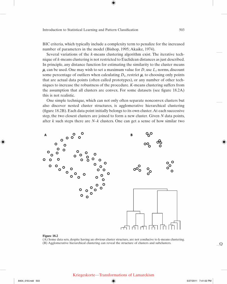
Several variations of the k-means clustering algorithm exist. The iterative tech-nique of k-means clustering is not restricted to Euclidean distances as just described. In principle, any distance function for estimating the similarity to the cluster means μc can be used. One may wish to set a maximum value for D, use L1 norms, discount some percentage of outliers when calculating Dk, restrict μc to choosing only points that are actual data points (often called prototypes), or any number of other tech-niques to increase the robustness of the procedure. K-means clustering suffers from the assumption that all clusters are convex. For some datasets (see figure 18.2A) this is not realistic.

One simple technique, which can not only often separate nonconvex clusters but also discover nested cluster structures, is agglomerative hierarchical clustering (figure 18.2B). Each data point initially belongs to its own cluster. At each successive step, the two closest clusters are joined to form a new cluster. Given N data points, after k such steps there are N–k clusters. One can get a sense of how similar two

Figure 18.2(A) Some data sets, despite having an obvious cluster structure, are not conducive to k-means clustering. (B) Agglomerative hierarchical clustering can reveal the structure of clusters and subclusters.

8404_018.indd 503 5/27/2011 7:41:02 PM

Q



points are by looking at when they were joined together into a cluster. The meaning of “closest clusters” is open to interpretation, but common choices include finding the pair of clusters with the shortest distance between any two points, the smallest average distance between points in each cluster, or the smallest distance between the farthest points in the two clusters. This straightforward and deterministic pro-cedure can be useful for getting an overview of the structure of the data.

Several more advanced clustering methods have been successfully applied to neuroscience problems. These include superparamagnetic clustering (in which the labels of points are probabilistically transmitted to nearby points, in a process inspired by the distribution of magnetic states at different temperatures) (Quian Quiroga et al., 2004), spectral clustering (in which distances between the data are used to create a weighted graph, and points are clustered based on the probability of a random walker transitioning between them), self-organizing Kohonen maps, and Gaussian mixture models, among others (Duda and Hart, 1973; Bishop, 1995; Hertz et al., 1992).

Supervised Learning

Many of the chapters in this book use supervised learning algorithms to decode the activity of populations of neurons (e.g., chapters 7 and 10). Here we provide an overview of several important supervised learning algorithms. In a typical situation, we have a dataset X={xi} (i=1,…,N and xi

d∈� ) and labels yi ∈ −{ , }1 1 —a binary classification scenario. We wish to divide the xi so that, as much as possible, they are separated according to their labels. Once this is done, the labels of new data can be “decoded” by where they lie in this space. For some datasets, it is possible to describe all or most of the “interesting” variation with one dimension. This may be the case when the data themselves are one-dimensional; more interesting are the cases in which the data are multidimensional, but some one-dimensional function of the data captures most of the “relevant” variation (as understood in the context of the clas-sification task). As emphasized in chapter 19, supervised learning involves separat-ing the data into two disjoint sets: a training set and a test set. How the data are divided into these two sets often depends on the questions under study (see more information in chapter 19). The training set is used to estimate the classification function (e.g., to compute w in the Linear Discriminant Analysis that follows). The test set is used to evaluate the performance of the classifier.

Linear Discriminant Analysis

The basic idea behind Linear Discriminant Analysis is to project the data onto a line in such a way that the projected data are well separated on that line. The trick is to find the best such line for a given definition of the classification error (see

8404_018.indd 504 5/27/2011 7:41:02 PM

Q



figure 18.3). The first property that we would like the chosen line to have is that it does a good job separating the data of the two classes. Separating their means seems like a good place to start. Let m+1 and m–1 be the means of the xi for which yi is 1 and –1, respectively. If w is the vector describing our line, we want to maximize the projected distance between m+1 and m–1; that is, find

�w w m m

w= ⋅ −+ −arg max ( )1 1

where “·” indicates the dot product operation. We will also need to find some value b that will discriminate between classes (discussed later). We then construct the “discriminant function” f b b( ; , )x w w x= + ⋅ . When f b( ; , )x w > 0, we label the point

Figure 18.3(A) The two classes of data (circles and stars), when projected onto the axis indicated, are easily sepa-rated by a point between the two clusters corresponding to the projections of the two classes. (B) A different projection yields a linearly inseparable mixture of the two classes. (C) 1. For this dataset, the line between the two class means does not yield a separable projection. 2. For the same dataset as in (c1), the axis dictated by Fisher’s linear discriminant allows us to easily separate the two projected classes.

8404_018.indd 505 5/27/2011 7:41:02 PM

Q



as +1, and when less than 0 we label the point as –1. Note that multiplying w and b by a constant c>0 does not change the discriminant function in any meaningfully way— f c cbi( ; , )x w has the same sign for any value of c and any xi. Our maximiza-tion task is therefore not well defined, as w m m⋅ −+ −( )1 1 can be made arbitrarily large by multiplying w by an arbitrarily large scalar. We therefore restrict w to be 1 and find �w w m m

w= ⋅ −+ −arg max ( )1 1 .

The solution is

wm mm m

=−−

+ −

+ −

1 1

1 1

,

the magnitude-one vector parallel to the line between the means.While projecting the two clusters of data onto the line between their means makes

intuitive sense, there are cases in which it is not appropriate (see figure 18.3C1). One common refinement of this technique, Fisher’s linear discriminant, attempts also to minimize the ratio of the difference in means to the spread within each projected cluster. Not only are we trying to separate the two groups of data, we are trying to describe each group as precisely as possible. Put another way, we are maxi-mizing the ratio of variance between projected groups to variance within projected groups. The numerator in Fisher’s criterion is the square of the difference between the projected means. The denominator is the sum of the projected variances for each class. Let G+ + += − −1 1 1( ).( )x m x mi i

Ti and G− − −= − −1 1 1( ).( )x m x mi i

Ti be

the covariance matrices for the +1 and –1 classes. The Fisher linear discriminant seeks to find the w that maximizes the following expression:

�w

w m mw ww

=⋅ −

++ −

+ −arg max

( ( )).( ).

T

T

1 12

1 1G G (18.3)

subject to w = 1 . It can be shown that this expression is minimized when:

G G+ − + −+( ) −1 1 1 1.w m m= (18.4)

In any linear discrimination problem, once we have decided upon a vector onto which we are projecting the data, we must then decide upon the boundary between classes, which is determined by b. We want a b that minimizes the classification error; hidden behind this straightforward goal are some considerations. First, how do we measure how bad an error is? Second, do we base the evaluation of classification error upon empirical data or upon inferred or assumed properties of the underlying distributions of the data? Minimizing classification error by minimizing misclassified empirical data is straightforward; optimizing the decision boundary based on prob-ability distributions takes us into the realm of decision theory.

8404_018.indd 506 5/27/2011 7:41:03 PM

Q



Neural Networks

Many classification algorithms, including the Fisher linear discriminant, can be readily interpreted and implemented through a neural network. Neural network classifiers are loosely modeled on real neurons. They are composed of intercon-nected units, each of which has a number of inputs. The strengths of those input connections are interpreted to correspond to synaptic strengths (or weights). The units in a neural network are typically arranged into multiple layers. The first layer is the input layer and the last layer is the output of the network (intermediate layers are often referred to as “hidden layers”). The “activity” of each unit is represented by a scalar value (loosely interpreted to represent the “firing rate” of the unit), denoted by aj

l( ) where (l) indicates the layer and j indicates the unit number within that layer. We denote the weight between unit i in the previous layer (l –1) and unit j in layer (l) by wji

l( )−1 . All the units in layer (l – 1) are connected to all the units in layer (l); however, some of the weights could take a value of 0. The activation aj

l( )

is computed from its inputs by taking the weighted sum of the inputs and applying an activation function:

a g w ajl

jil

il

i

d l( ) ( ) ( )

( )

=

− −

=

−

∑ 1 1

0

1

(18.5)

where typically a l0

1 1( )− = and wjl0

1( )− is a constant bias term for all the units in layer (l), g() is a nonlinear activation function and d(l –1) is the number of units in layer (l – 1). For the input layer (l = 0), a xj j

( )0 = , where xj is the jth dimension of the input. The weighted sum of all inputs is reminiscent of what happens in the soma of a neuron as it integrates inputs from its many dendrites. The activation function is often interpreted as the transformation between the weighted summed input to a neuron (loosely thought of as the intracellular voltage at the soma) and its output firing rate. The most common activation functions are sigmoids such as the hyper-bolic tangent and the log-sigmoid

g ze z

( ) =+ −

11

.

A schematic of a typical neural network architecture is shown in figure 18.4. The Fisher linear discriminant discussed earlier can be easily mapped to a two-layer network with a linear activation function.

There are two aspects to constructing a neural network to solve a problem. The first is to determine a network architecture (number of layers, number of units in each layer); once this is done, the network must be trained, a process by which the weights of the network are iteratively updated so that the network better accom-plishes the training objective. Neural networks generalize to label sets with more than two elements in a more straightforward manner than many other classifiers. Multidimensional binary labels such as (1, 0, 1, 1, 0) can be represented by training

8404_018.indd 507 5/27/2011 7:41:03 PM

gabrielkreiman

Cross-Out

Q



a network with, in this example, five units in the output layer with binary activation functions. Multiclass labels, such as those drawn from {1, 2, 3, 4}, can be represented by a single output neuron with an activation function whose range includes the desired values. It is often more successful, however, to use output coding whereby each possible class is represented by a single output unit whose value is either 0 or 1. It is also possible to use a neural network for regression, with a linear activation function in the last layer.

Deciding on the structure of a neural network has been called a black art. The number of outputs of the network, equivalent to the number of units in the highest layer, is determined as noted by the problem being solved. The number of inputs to the network, and hence the number of inputs to each unit in the first layer, is simi-larly constrained by the dimensionality of the data (see the preceding discussion and also the one in chapter 19 about feature extraction and dimensionality reduc-tion). The number of “hidden” layers between the input and output is up to the user, as is the number of units in all layers save the highest. A very common architecture, however, involves a relatively large input layer, a single hidden layer with a smaller number of units (though each layer must have enough units to adequately represent

Figure 18.4A small neural network with a four-dimensional input layer, a single two-dimensional hidden layer, and a three-dimensional output layer.

8404_018.indd 508 5/27/2011 7:41:03 PM

Q



the important dimensions of the data), and an output layer whose unit count is determined by the desired form of the output—one, for a binary classification problem.

The weights of a neural network are updated using algorithms such as backpropa-gation (Bishop, 1995). In this algorithm, the weights are updated through successive iterations according to the gradient of the empirical risk surface (“gradient descent”). This algorithm is guaranteed to converge to a local minimum of the risk surface. While the backpropagation procedure is guaranteed to converge to a local minimum in the empirical risk surface, it may take a very long time to do so. It is also some-times the case that the discovered local minimum is significantly worse than the desired global minimum. Several techniques exist to ameliorate both of these chal-lenges. Often, the weight updates are modified by some weighted sum of the recent updates (a momentum term) to speed convergence and help avoid getting stuck in small “pits” in the error surface. The initial state of the weights can exert tremendous influence on the results, so when beginning with random weights it is generally a good idea to train many networks and use the best. Heuristics also exist to set the weights to initial values that are likely to be close to the global minimum of the risk surface (Vapnik, 1995; Bishop, 1995).

Support Vector Machines

Support Vector Machines (SVM) constitute a powerful and often used approach to supervised learning problems (Cristianini and Shawe-Taylor, 2000; Vapnik, 1995). They have proven to be quite effective and robust in a variety of learning problems and are increasingly used in decoding approaches in neuroscience. We focus here on the binary classification problem where we have labeled data examples (xi, yi), yi ∈ −{ }1 1; . SVMs seek to separate the two classes by finding a hyperplane that is as far as possible from the closest data points. SVMs allow for complex nonlinear discriminations to be made in higher dimensional spaces while controlling general-ization to avoid overfitting.

This distance from the data to the separating hyperplane is quantified by the “margin” of the hyperplane. The margin is the sum of the distance to the closest point with a label of +1 and the distance to the closest point with a label of –1. In other words, the amount of space around the separating hyperplane, before you start hitting data points. Those points at this minimum distance are the “support vectors,” and describe two other parallel marginal hyperplanes bounding the margin. If the data are linearly separable, there is a hyperplane that separates the two classes, described by w xT b+ = 0 , where w is a vector normal to the hyperplane and −b / w is the distance to the origin. Note that y bi

Ti( ) /w x w+ is the perpendicular dis-

tance from the hyperplane to a correctly classified point xi (for incorrectly classified points this value is negative), and if the data are correctly separated by this hyper-

8404_018.indd 509 5/27/2011 7:41:03 PM

Q



plane we have that y biT

i( )w x + > 0 for all (xi, yi). The problem of finding the hyper-plane that induces the maximum margin is solved by minimizing w 2 subject to y bi

Ti( )w x + ≥ 1. This is done by using the technique of Lagrange multipliers to

search for the �w and

�b that minimize w 2, thereby maximizing the margin. Once

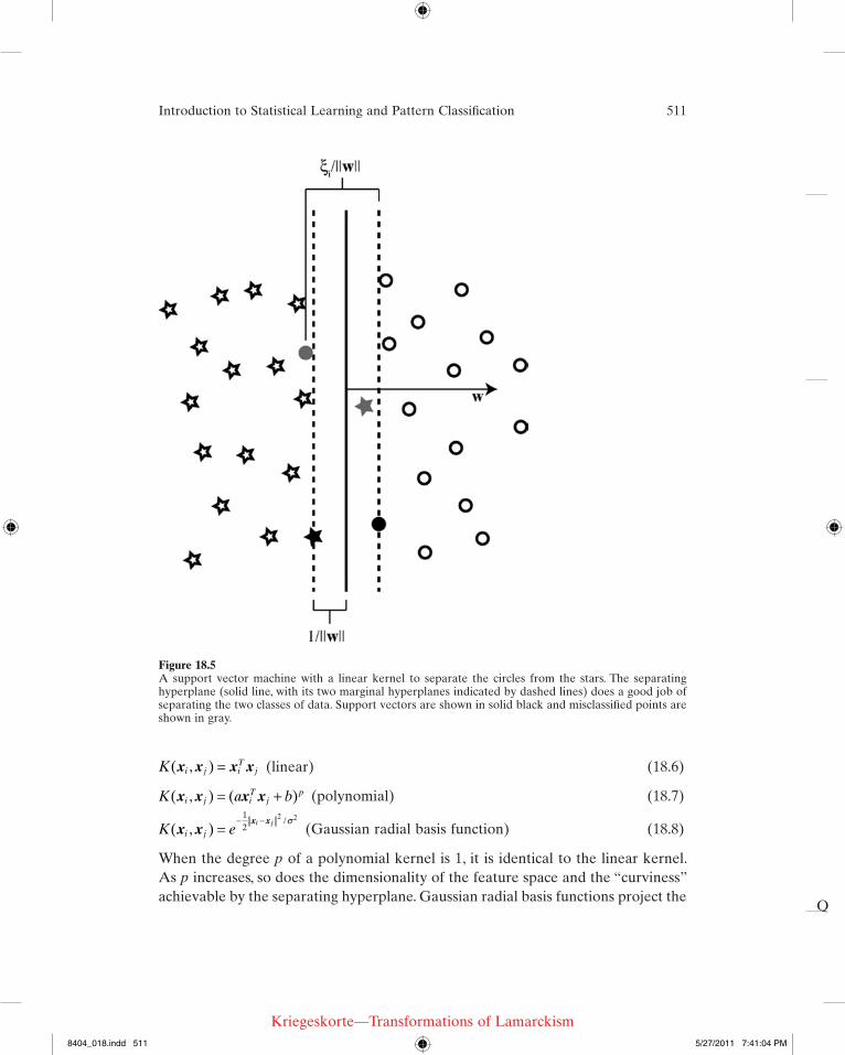
this separating hyperplane is found, evaluating the class of a new datum x is as simple as determining on which side of the hyperplane it lies, as given by the sign of � �b T+ w x. These values are illustrated in the case of a two-dimensional SVM in

figure 18.5.In the real world, and in particular in neuroscience, many datasets are not linearly

separable. Fortunately, there are enhancements to the basic maximum-margin hyperplane technique that allow SVMs to function under such conditions. First, one may permit some of the points to be misclassified. Of course, it is better to avoid this if possible, so we discourage it by penalizing it. Each point xi is associated with a “slack variable” ξi, which measures how far past the marginal hyperplane the point is. When ξi is greater than 0, xi is on the wrong side of the marginal hyperplane. When ξi is greater than 1, xi is misclassified—it is on the wrong side of the separating hyperplane. We incorporate the ξi into our previous constraint and solve the problem by minimizing w 2 2/ + ∑C i

i

ξ subject to y biT

i i( )w x + + ≥ξ 1 and (ξi ≥ 0). C is a regularization constant that regulates how stiff the penalties are for incorrect clas-sification and is typically optimized empirically.

Adding slack variables allows us to classify noisy datasets that, in the absence of noise, would be linearly separable. Some datasets, however, cannot even in principle be separated by a straight hyperplane. For these cases, we can remap the data into a new space (a “feature space”) in which they are linearly separable (or close to it—we will keep slack variables so that we do not overfit to noise). We first need some function Φ : � �d H that maps our data into the feature space H. To be useful, H is typically of higher dimension than the original data. To accomplish training of these remapped higher-dimensional values in a computationally tracta-ble way, we take advantage of the fact that the optimization problem solved in training only involves the training data as dot products of pairs of data points, x xT

i j⋅ . This means that the training on the remapped data needs expressions form of Φ Φ( ) ( )x xi

Tj⋅ —once this expression is evaluated, it is one-dimensional. For

certain classes of functions (Cristianini and Shawe-Taylor, 2000), there exists another function K (the “kernel function”) such that K i j i

Tj( , ) ( ) ( )x x x x= ⋅Φ Φ . These kernels

measure the similarity between two input vectors. Using this “kernel trick” implies that we do not ever need to compute Φ( )x ; all we need is to be able to compute the NxN kernel matrix K i j( , )x x . Training a classifier in feature space then depends only on the evaluation of this kernel function. This can cut out a huge number of calculations that would otherwise be very expensive, particularly in the case of an infinite-dimensional feature space. Several kernel functions are commonly used:

8404_018.indd 510 5/27/2011 7:41:03 PM

Q



K i j iT

j( , )x x x x= (linear) (18.6)

K a bi j iT

jp( , ) ( )x x x x= + (polynomial) (18.7)

K ei ji j

( , )/

x xx x

=− −1

22 2σ

(Gaussian radial basis function) (18.8)

When the degree p of a polynomial kernel is 1, it is identical to the linear kernel. As p increases, so does the dimensionality of the feature space and the “curviness” achievable by the separating hyperplane. Gaussian radial basis functions project the

Figure 18.5A support vector machine with a linear kernel to separate the circles from the stars. The separating hyperplane (solid line, with its two marginal hyperplanes indicated by dashed lines) does a good job of separating the two classes of data. Support vectors are shown in solid black and misclassified points are shown in gray.

8404_018.indd 511 5/27/2011 7:41:04 PM

Q



input data into an infinite-dimensional feature space; a lower standard deviation σ gives a greater ability to specify convoluted separations between data classes.

The kernel parameters are often optimized empirically by using a subset of the data (training set) to avoid overfitting. We use the same kernel trick for evaluating new data. Classifying a new data point x depends on the dot product �w xT , for which we use our kernel function rather than projecting x into feature space. Abstracting away the feature map with a kernel is incredibly powerful; not only does it save us from having to evaluate and optimize high-dimensional func-tions, but it also allows us to disregard the feature map and consider only the kernel function. When describing SVMs, therefore, people speak in terms of the kernel used rather than the feature map. In fact, while a given feature map dictates a kernel, a given kernel does not specify a particular feature map (or even a particular feature space).

Bias versus Variance

A theme central to all of machine learning is the tradeoff between minimizing bias and minimizing variance. An estimator

�θN is a function on size-N sets of data that

returns an estimate �θ of some property θ (such as the mean) of those data. In

general, the bias of an estimator is the expected deviation (over all possible datasets) from the true value:

bias( ) ( )� �θ θ θN

XNE

N= − .

An unbiased estimator, in other words, yields an estimate that on average is equal to the true value. The sample mean, for example, is an unbiased estimator of the actual mean of a distribution.

By using more complex models with more free parameters, it is possible to find lower-bias estimators. Unfortunately, these models require more data to fit properly. For a given dataset size, therefore, the estimator will have a higher variance. Simpler models, on the other hand, can be fit well with fewer points and therefore have a lower variance; the cost is a higher bias. The two are related to each other and to the overall risk as follows:

E N N N( ) ( ) var( )� � �θ θ θ θ− = +2 bias2 .

The bias term is intrinsic to the estimator, and the variance term reflects how sensi-tive the estimator is to the data. One of the most important tasks in a machine-learning problem is to choose a model of appropriate complexity given the distributions and quantity of data. It is also important, experimentally, to ensure that the quantity of data is sufficient to support classification.

8404_018.indd 512 5/27/2011 7:41:04 PM

Q



To put this issue in more concrete terms, an overly complex classifier will tend to do a very good job of separating a given dataset. It will have a low empirical risk (the manifestation for a classifier of the bias term in the equation relating bias and variance of an estimator). However, it is likely to accomplish this in a manner par-ticular to that dataset, which does not generalize to other datasets. In a word, it overfits; the confidence interval (the manifestation of the variance term for a clas-sifier) describing how close we are likely to be to the true class boundary is large. An overly simple classifier, on the other hand, will fail to accommodate real nuances in the dataset and will therefore also perform in a suboptimal manner. Figure 18.6 illustrates classifier boundaries that are too simple and too complex for the data.

In the best case, we would like to find a classifier that minimizes the overall risk. Neural networks and SVMs take complementary approaches to this problem. For a given neural network architecture, the confidence interval is fixed—the potential sensitivity to different data is intrinsic to the network architecture. The weights of the network are then tuned so as to minimize the empirical risk. SVMs instead aim to maximize the generalization power to new data by maximizing the margin (see above). It is not generally possible to know in advance the optimal complexity of classifier to use. Often, one must try many different choices of parameters (neural network architectures or kernel function parameters) in a search for the values that optimize the performance (using the training data). Testing classifier performance on the same dataset used to train it will reward very complex models that individu-ally describe each data point but are unable to generalize to new data. Instead, classifiers are usually tested using some variant of a leave-n-out strategy (see chapter 19 for further discussion of cross-validation). The data are partitioned, some data are used for training, and the classifier’s performance is then evaluated on the rest. This process is repeated for many different partitions of the data to get a good idea of the overall performance of the classifier.

Generalization Theory

It is possible to describe the capabilities of a classifier with greater rigor, and even get numerical bounds on the error as a function of the number of data points. The basic idea is that of “probably approximately correct” (PAC) learning. We want to know that there is only a small chance δ that a classifier generated with a given technique on a dataset of size N has error greater than some bound ε.

We can view a classification technique, with its corresponding parameters, as a set H of hypotheses h, functions that map from the space the data occupy to the space of classes (say, {–1, +1}). The goal of classifier training is to pick an appropriate h; here, however, we are concerned with picking an appropriate H, that is choosing the form that the classifier will take (whether this be the structure of a neural

8404_018.indd 513 5/27/2011 7:41:04 PM

Q



network, the standard deviation of the radial basis functions in an SVM, or any other such question). We will describe the capacity, the ability to fit complex data, of a class H with a value known as the VC dimension of the class (named for Vapnik and Chervonenkis).

A hypothesis class H is said to shatter a set of points {x1,…, xN} if it is possible to achieve any of the 2N possible classifications (that is, vectors of length N whose ele-ments are either +1 or –1) using only hypotheses within H. Some hypothesis classes are rich enough that they can shatter sets of points of any size; these are said to have infinite VC dimension. For others, there is some largest set size d that can be shattered by H. The VC dimension is this largest set size d, a measure of how complex a set of data one can represent with H. Furthermore, a fundamental theorem in learning theory, due to Vapnik and Chervonenkis, states the following:

Assume H has VC dimension d, and the number of data N in a sample is greater than d. Then for any hypothesis h in H, if h classifies that sample of size N cor-rectly then there is probability 1-δ that the expected error over all samples is no more than ε δ= +( )2 2 2

NeNdd ln ln as long as N > 2 / ε. In other words, given that we

know something about the richness of the classifier that we are using, we know that if it classifies a large enough dataset it is probably approximately correct with respect to the underlying distribution from which the data were generated. We can even have numerical values for “large enough,” “probably,” and “approximately.” Further refinements give similar results in the case where h classifies the data mostly correctly. This concept of VC dimension also explains why SVMs are able to achieve good generalization performance rather than overfitting, despite working with data projected into a feature space that is often of very high dimension (or even infinite dimension). For example, a radial basis function SVM works with an

Figure 18.6(A) A classification bound with low empirical risk but large confidence interval; this bound likely suffers from overfitting. (B) A classification bound with high empirical risk but low confidence interval; this bound fails to accommodate the details of the boundary between the two classes. (C) An intermediate classification bound that does a good job of separating the actual data without being ruled by details that are likely particular to this sample.

8404_018.indd 514 5/27/2011 7:41:04 PM

Q



infinite-dimensional kernel space, but has a finite VC dimension that depends inversely on σ.

Implications for Neuroscience

Neuroscience data can be noisy, complex, and difficult to understand. Compounding this by recording many channels at once can make analysis seem a daunting task. The advances in computational statistics that have been made in the last half-century allow us extract patterns from complex multidimensional datasets. The experiments described in the main chapters of this book have often made use of these techniques. Between their examples and the details provided in these appendices, we hope that the interested reader can see ways to extend analysis of his or her own data.

Supervised learning techniques such as SVMs can help quantify the amount of information about visual stimuli that are conveyed by a neuronal population. This does not imply that the brain uses the same SVM algorithms for learning the cor-responding hyperplanes. Regardless of the mechanisms that cortex might use to learn the set of weights w, once learnt, many of the classification boundaries can be described by relatively simple expressions (e.g. a linear dot product followed by a nonlinearity) that could be implemented by biological hardware.

Some Links

We provide a non-exhaustive list of links that may help the user interested in imple-menting and/or using some of the ideas in this chapter. For an expanded and updated list of links, see also http://klab.tch.harvard.edu/multivariate.html.

1. http://www.nr.com/ Numerical Recipes (The Art of Scientific Computing)

2. http://cbcl.mit.edu/software-datasets/index.html

Center for Biological and Computational Learning at MIT

3. http://www.support-vector-machines.org/

Literature and links to SVM software

4. http://www.mathworks.com/matlabcentral/fileexchange/

MATLAB File Exchange. Beware, there is good stuff and bad stuff.

5. http://sccn.ucsd.edu/eeglab/ EEGLAB: a MATLAB toolbox for performing ICA and many other analyses on multichannel data.

6. http://www.cpu.bcm.edu/laconte/3dsvm.html

AFNI 3dsvm plug-in

8404_018.indd 515 5/27/2011 7:41:04 PM

Q



7. http://code.google.com/p/princeton-mvpa-toolbox/

Princeton MVPA toolbox

8. http://pkg-exppsy.alioth.debian.org/pymvpa/

PyMVPA toolbox

9. http://www.csie.ntu.edu.tw/~cjlin/libsvm LIBSVM toolbox

10. http://www.ibtb.org/ Panzeri’s toolbox

11. http://code.google.com/p/pyentropy/ Panzeris’ toolbox

References

Akaike H. 1974. A new look at the statistical model identification. IEEE Trans Automat Contr 19: 716–723.

Bishop CM. 1995. Neural networks for pattern recognition. Oxford: Clarendon Press.

Cristianini N, Shawe-Taylor J. 2000. An introduction to support vector machines: and other kernel-based learning methods. Cambridge: Cambridge University Press.

Duda RO, Hart PE. 1973. Pattern classification and scene analysis. New York: Wiley-Interscience.

Gabbiani F, Cox SJ. 2010. Mathematics for Neuroscientists. London, UK Academic Press.

Hertz J, Krogh A, & Palmer R. 1992. Introduction to the theory of neural computation. Santa Fe, NM: Santa Fe Institute Studies in the Sciences of Complexity.

Hyvarinen A, Oja E. 2000. Independent component analysis: algorithms and applications. Neural Netw 13(4–5): 411–430.

Jung T-P, Makeig S, Mckeown MJ, Bell AJ, Lee T, Sejnowski TJ. 2001. Imaging brain dynamics using independent component analysis. IEEE Proceedings 88(7): 1107–1122.

Lewicki MS. 1998. A review of methods of spike sorting: the detection and classification of neural action potentials. Network 9: R53–R78.

Poggio T, Smale S. 2003. The mathematics of learning: dealing with data. Notices AMS 50: 537–544.

Poggio T, Rifkin R, Mukherjee S, Niyogi P. 2004. General conditions for predictivity in learning theory. Nature 428: 419–422.

Press WH, Teukolsky SA, Vetterling WT, Flannery BP. 1996. Numerical recipes in C. 2nd ed. Cambridge: Cambridge University Press.

Quian Quiroga R, Nadasdy N, Ben-Shaul Y. 2004. Unsupervised spike sorting with wavelets and super-paramagnetic clustering. Neural Comput 16: 1661–1687.

Vapnik V. 1995. The nature of statistical learning theory. New York: Springer.

8404_018.indd 516 5/27/2011 7:41:04 PM

Jed Singer and Gabriel Kreiman Summary - Harvard...

Documents

Transcript of Jed Singer and Gabriel Kreiman Summary - Harvard...