J.D. Bramble, Ph.D. Creighton University Medical Center Med 483 -- Fall 2005 Confidence Intervals.

J.D. Bramble, Ph.D.Creighton University Medical

CenterMed 483 -- Fall 2005

Confidence Intervals

J.D. Bramble, Ph.D.MED 483 – Fall 2005


Data can be described by point estimates mean, standard deviation, etc.

Point estimates from a sample are not always equal to population parameters

Data can be described by interval estimates shows the variability of the estimate.

Using the standard error we can see the amount that the estimate will vary from the true value.



Interval estimates are called confidence intervals (CI).

CI define the an upper limit and lower limit associated with a known probability.

These limits are known as confidence limits.

The associated probability of the CI is most commonly 95%, but may be 99% or 90%


Confidence limits set the boundaries that are likely to include the population mean.

Thus, we can conclude that in general, we are 95% confident that the true mean of the population is found within these limits.



Standard Error

The standard error is defined as We expect that the mean is within one

standard error of quite often. SE is a measure of the precision of x as an

estimate of . The smaller SE the more precise the estimate

SE includes two factors that affect the precision of the measurement n and sd

n

s


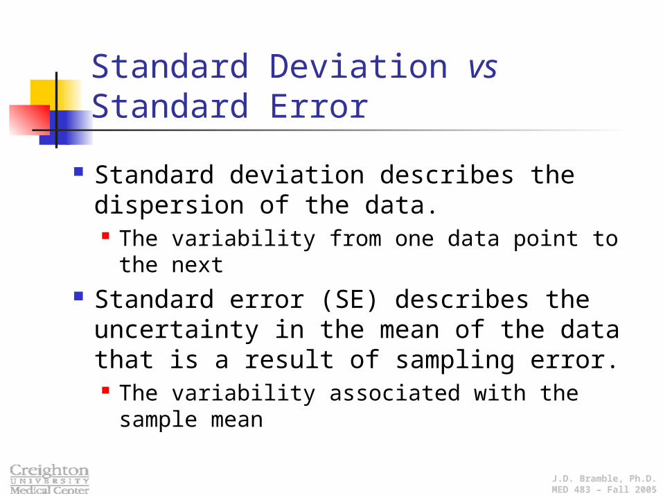
Standard Deviation vs Standard Error

Standard deviation describes the dispersion of the data. The variability from one data point to the next

Standard error (SE) describes the uncertainty in the mean of the data that is a result of sampling error. The variability associated with the sample mean


Calculating Confidence Intervals

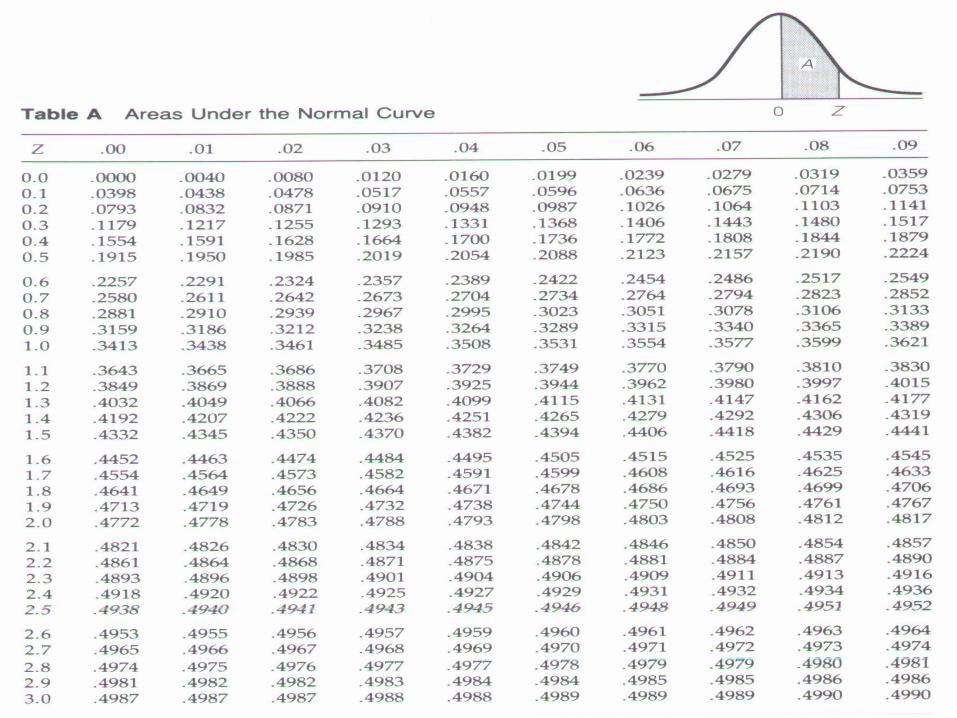
Recall that 95% of the area under a standard curve is between z = ±1.96.

-1.96 1.96

95.45%


Calculating Confidence Intervals

The general formula is:

P = 0.95

Lower limit = x - 1.96( n ) Upper limit = x + 1.96 ( n )

n

zx

n

zx


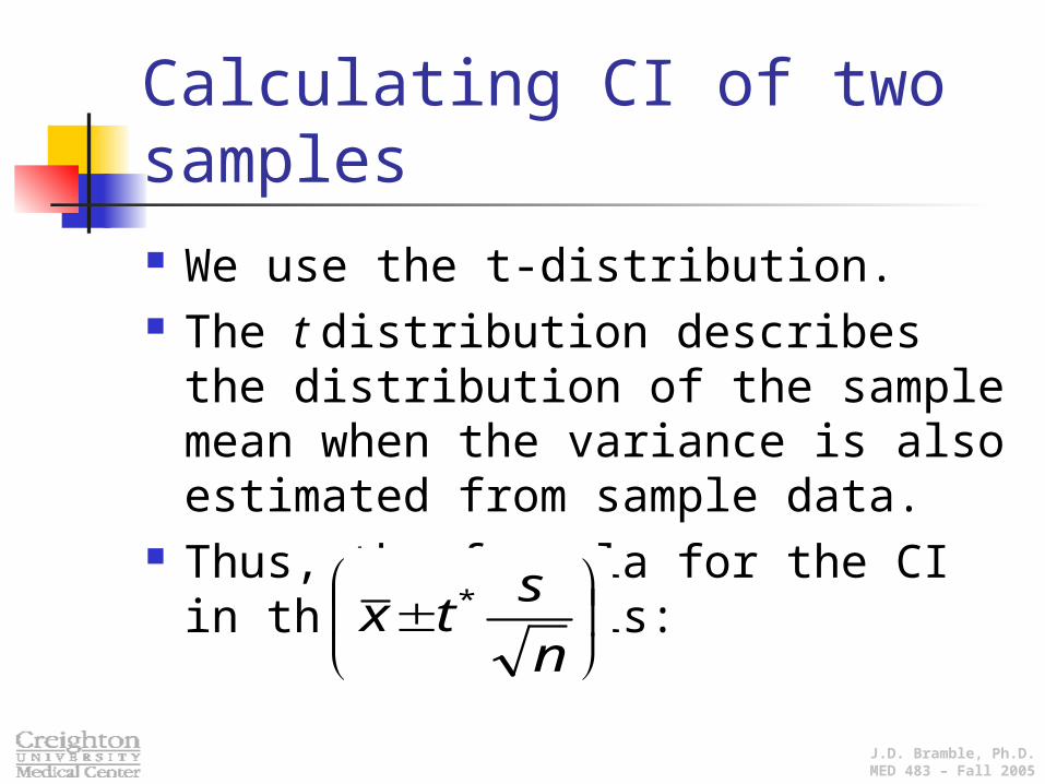
Calculating CI of two samples We use the t-distribution. The t distribution describes the distribution

of the sample mean when the variance is also estimated from sample data.

Thus, the formula for the CI in these cases is:

n

stx *


Example: Problem To assess the effectiveness of hormone replacement

therapy on bone mineral density, 94 women between the age of 45 and 64 were given estrogen medication. After taking the medication for 36 months the bone mineral density was measured for each of the women in the study. The average density was 0.878 g/cm2 with a standard deviation of 0.126 g/cm2. Calculate a 95% CI for the mineral bone density of this population.


Example: SE and t Recall that SE is:

t(, df) = t(0.025, 93) = 1.990

013.094

126.0

n

s


Example: Calculations

0.904 to0.852

0.2586 878.0

94

126.099.1878.0


Example: Conclusion

The 95% confidence limits are: lower: 0.852 g/cm2; upper: 0.904 g/cm2

We are 95% confident that the average bone density of all women age 45 to 64 who take this hormone replacement medication is between 0.852 g/cm2 and 0.904 g/cm2.


For a 95% confidence intervals we believe that 95% of the samples drawn form the population would have a mean that fall within the confidence limits

Example: Conclusions (cont’d)


Other Confidence Limits

For a 99% or 90% CI the calculations and interpretations are similar.

What CI is going to give the widest or narrowest interval?

CI can be established for any parameter mean, proportion, relative risk, odds ratio, etc.


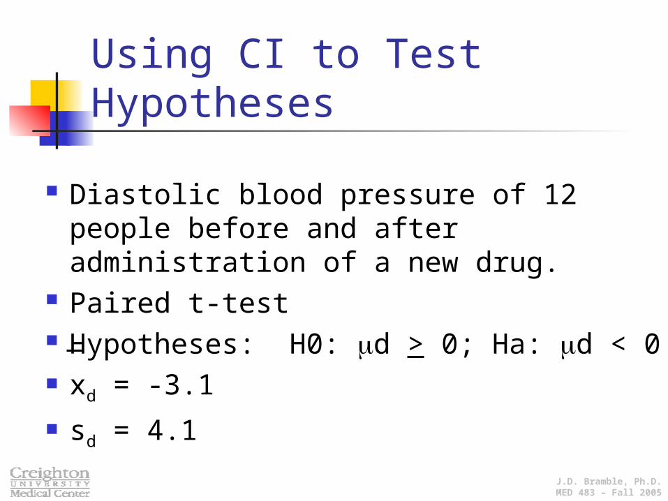
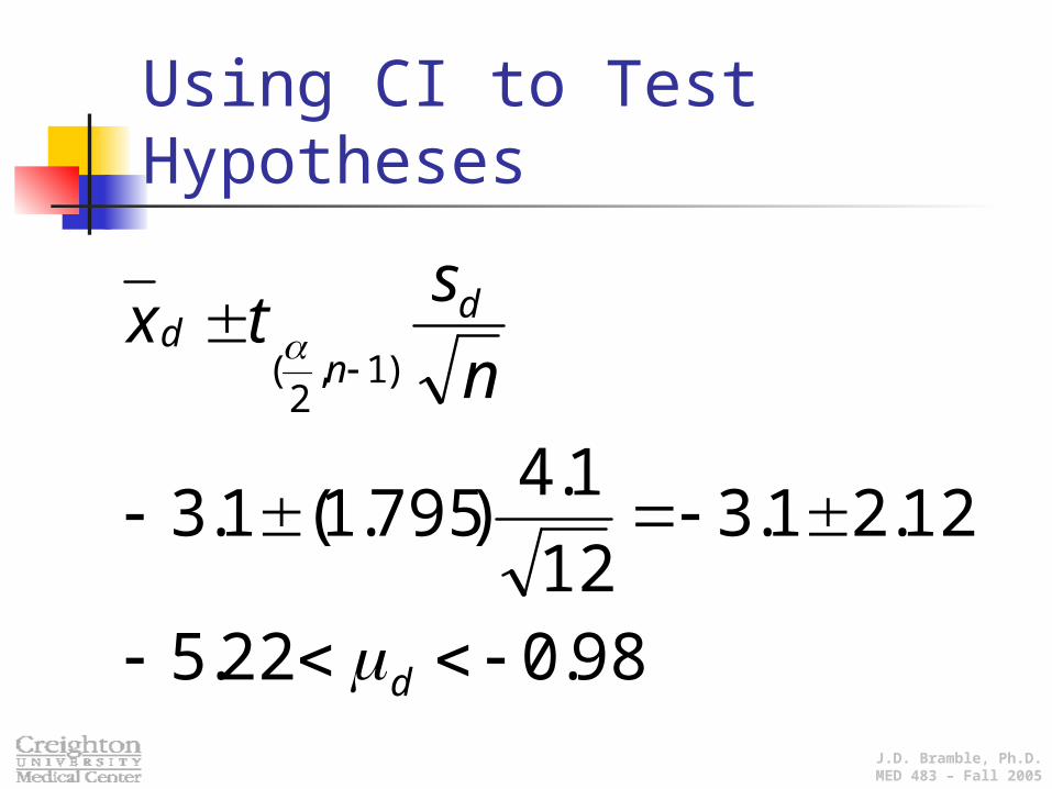
Using CI to Test Hypotheses

Diastolic blood pressure of 12 people before and after administration of a new drug.

Paired t-test Hypotheses: H0: d > 0; Ha: d < 0 xd = -3.1

sd = 4.1


98.022.5

12.21.312

1.4)795.1(1.3

)1,2

(

d

d

nd

n

stx



Conclusion – since zero does not fall within the interval we can conclude with 95% certainty that there is a significant decrease in blood pressure after taking the new drug.

If we did a paired t-test the conclusions would be the same.



]

]

]

]

]

]

]

]

]

]

]

[

[

[

[

[

[

[

[

[

[

[

True Population Mean ()

1

2

3

4

5

67

8

9

10

11

CI for different samples

Visual Representation of CI



ANOVA: Analysis of Variance

Single Factor


Objectives

Know the assumptions for an ANOVA When is ANOVA used rather than a t-test Set up ANOVA tables and understand the relationships

between the values within the table Compute the F-ratio and appropriate degrees of

freedom Know how and when to use a two factor ANOVA Apply Tukey’s multiple comparison procedure


A statistical method of comparing means of different groups.

A single factor ANOVA for two groups produces the same p-value as an independent t-test

The t-test is inappropriate for more than two groups – increases probability of a Type I error

Using a t-test to test the means of each pair leads to problems regarding the proper level of significance.

ANOVA vs. t-test


ANOVA is not limited to two groups Can appropriately handle comparisons of

several means from several groups Thus, ANOVA overcomes the difficulty of

doing multiple t-tests The sampling distribution used is the F

distribution.

ANOVA vs. t-test


ANOVA: assumptions

The observations are independent one observation is not correlated with another observation.

Variance of the various groups are homogeneous

ANOVA is a robust test that is not as sensitive to departures from normality and homogeneity, especially when sample sizes are large and nearly equal for each group.


ANOVA: Characteristics

ANOVA analyzes the variance of the groups to evaluate differences in the mean.

Within group Measures the variance of observations within each

group variance due to “chance”

Between groups measure the variance between the groups variance due to treatment or chance


ANOVA: Characteristics

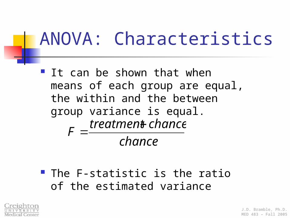
It can be shown that when means of each group are equal, the within and the between group variance is equal.

The F-statistic is the ratio of the estimated variance

chance

chancetreatmentF


ANOVA : the F distribution

The ratio follows an F distribution The F statistic has two sets of degrees of

freedom. For between groups -- (I - 1); where I is the

number of groups For within groups -- I(J - 1); where J is the

number of observations in each group


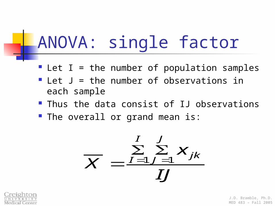
ANOVA: single factor Let I = the number of population samples Let J = the number of observations in each sample Thus the data consist of IJ observations The overall or grand mean is:

IJ

xX

jk

J

J

I

I 11


Now it is necessary to compute the sums of squares for the treatment -- SSTr (between group); error--SSE (within group), and the total-- SST.

Sum of the squared deviations between groups The total sums of squares measures the amount of

variation about the grand mean With algebraic manipulation we find that:

SST = SSTr + SSE

ANOVA: single factor


22

11

2 11)( x

IJx

JxxSSTr IJ

J

J

I

IIJ

22

11

2 1)( x

IJxxxSST IJ

J

J

I

IIJ

When completing the ANOVA table usually only SSTr and SST are calculated. SSE is found by SSE = SST - SSTr

ANOVA: sums of squared


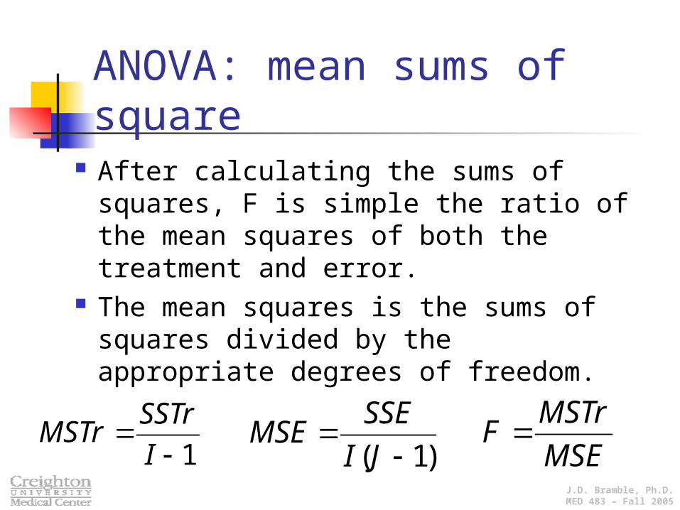
After calculating the sums of squares, F is simple the ratio of the mean squares of both the treatment and error.

The mean squares is the sums of squares divided by the appropriate degrees of freedom.

1

I

SSTrMSTr

)1(

JI

SSEMSE

MSE

MSTrF

ANOVA: mean sums of square


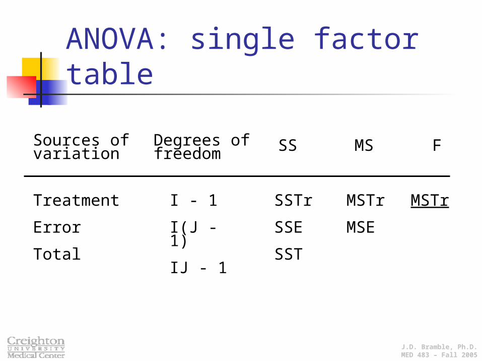
ANOVA: single factor table

Sources of variation

Degrees of freedom SS MS F

Treatment

Error

Total

I - 1

I(J - 1)

IJ - 1

SSTr

SSE

SST

MSTr

MSE

MSTr

MSE


ANOVA: Example

An experiment was conducted to examine various modes of medication delivery. A total of 15 subjects diagnosed with the flu were enrolled and the length of time until alleviation of major symptoms was measured for three groups: Group A received an inhaled version, Group B received an injection, and Group C received an oral dose.


Single factor example

x =

Groups A B C

56 62 72

102 58 100

Time (min) 90 78 117

87 68 109

94 87 103

Average 85.8 70.6 100.2


H0: all three means are equal or 1 = 2 = 3

Ha: at least one mean is different

= 0.05

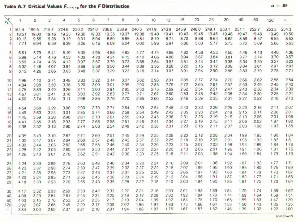
Critical value: F(, df) given I-1 = 2 and I(J-1) = 12, F(0.05, 2,12) = 3.89

Single factor example: set up


Single factor example: calculating sums of squares

7.153,53.739,109893,11415/)1283(893,114 2 SST

8.962,2128315

1])501()353()429[(

5

1 2222 SSTr

9.190,28.962,23.153,5 SSE


Single factor example: completing the table

Sources of variation

Degrees of freedom SS MS F

Treatments

Error

Total

2

12

14

2,190.3

2,962.8

5,153.7

1,095.5

246.9

4.44


Single factor example: decision and conclusions

Compare Fstat to Fcrit: 4.45 > 3.89, therefore fail to reject H0.

There evidence suggest that the time it takes to alleviate major flu symptoms differed significantly due to the mode of medication delivery.


Where is the Difference?

Recall the hypotheses of the ANOVA Ho is that all the means are equal Ha is that at least on is not.

If we fail to reject Ho the analysis is complete. What does it mean when Ho is rejected

at least one mean is different Which 's are different from one another.

if only two treatment levels. three or more treatment levels


Finding the difference We must do a post hoc analysis.

a test that is done after the ANOVA The purpose is to determine the location of

the difference. Different of post hoc test are available and

are discussed in the text. These test include Bonferroni, Sceffe,

Student Newman-Keuls, and Tukey' HSD.


Tukey’s HSD

Where, = significance levelI = number of groups

J = number of observation per treatment

MSE = mean square error (or within group MS)

J

MSEQw JII *))1(,,


Using the Tukey’s HSD

All the information, except Q, needed to find w is located in the ANOVA table

Q is determined by using the studentized range distribution, and dfwithin.

Once w is determined order all treatment level means in ascending order

Underline those values that differ by less than w. Treatment means not underlined correspond to

treatments that are significantly different.


Example Using the previous example, we no want to find which

form(s) of medication really is different form the others. To start we will order the means

Groups B A C

Average 70.6 85.8 100.2


The ANOVA Does this data indicate that the amount of time it takes a

student to nod off is dependent on the statistical topic being studied?

Source df SS MS F

Treatment (i.e., between) 3 5882.4 1960.8 21.09

Error (i.e., within) 16 1487.4 93Total 19 7369.8

Since the computed F-statistic of 21.09 is greater than the critical value of F(0.05, 3, 16) = 3.24 we reject Ho.


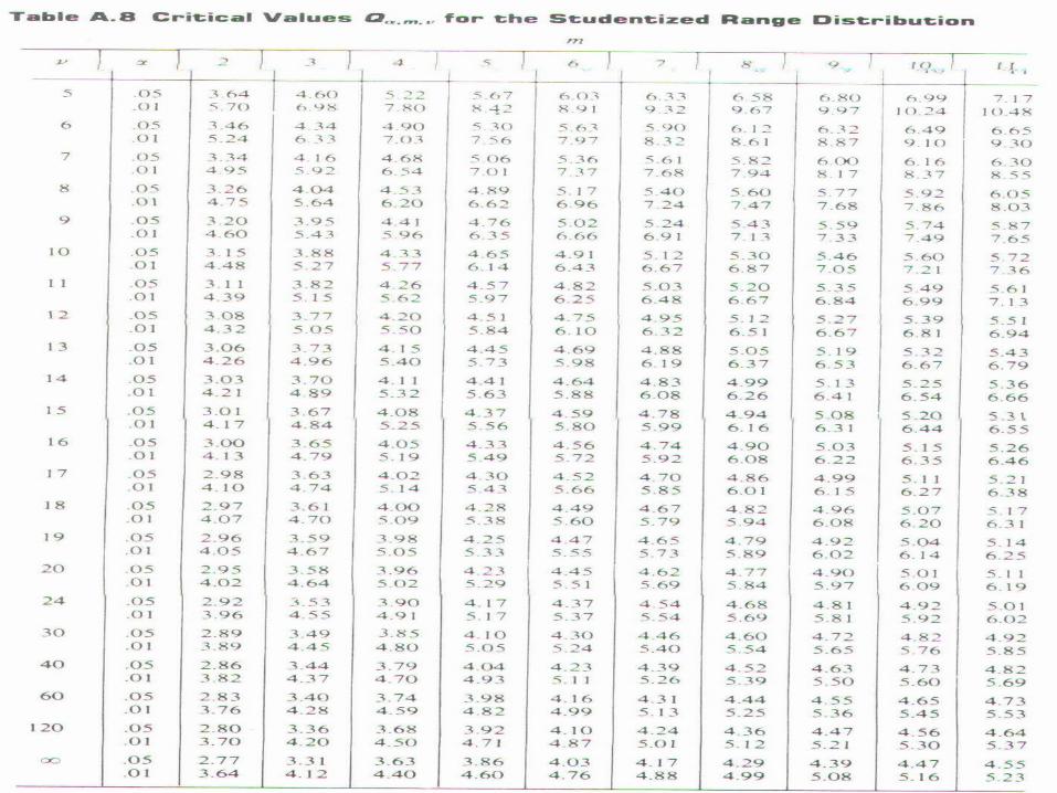
Computing the Tukey’s There are I = 3 treatments and the degrees of

freedom for the error is 12; thus, from the table Q(0.05, 3, 12) = 3.77.

Computing the Tukey value we get:

5.265

9.246*77.3*)1(,,( J

MSEQ JII


And the Difference is…

Ordering the treatment level means and underscoring those that differ by less that 26.5

We conclude that only significant difference is between group B (injection) and group C (oral).

Groups B A C

Average 70.6 85.8 100.2



ANOVA: Analysis of Variance

Two Factor


Two-Factor ANOVA

Single factor ANOVAs subjects or treatments are categorized in only

one way (i.e., type of treatment) Two factor ANOVAs

subjects or treatments are categorized in two ways (i.e., type of treatment and gender)

Two factor ANOVAs test the influence of both factors.


Examples of Two Factor Designs

An experiment is designed to test if there is a difference in how fast 3 different antacid brands (Acid Eater, Relieve the Burn, and Blah Stomach) dissolve in male and female stomachs.

What type of study techniques (1 hour every day, 3 hours once a week, an "all-nighter" prior to the exam, a late night party before the exam) results in better test scores while controlling for the person's age (<17, 18-20, 21-23, 24-26, 27 >).


Advantages of Two-way ANOVAs

Economy In a two-factor analysis we can test

interactions. Testing for an interaction allows us to

determine whether the variation of the treatment varies by the conditions in which the treatment is applied


Example

Instruction

Computer Classroom Means

Ability Whiz 90 82 86

Novice 80 88 84

Means 85 85


Three Research Hypotheses

Is there a significant difference between those taught by computer and those taught in the classroom?

Is there a significant difference between computer whizzes and computer novices

Is there a significant interaction between type of instruction and computer ability of the subject


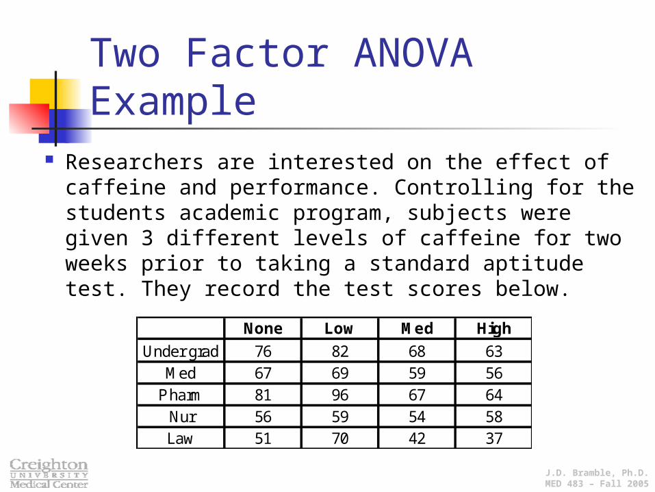
Two Factor ANOVA Example

Researchers are interested on the effect of caffeine and performance. Controlling for the students academic program, subjects were given 3 different levels of caffeine for two weeks prior to taking a standard aptitude test. They record the test scores below.

None Low Med High

Under grad 76 82 68 63Med 67 69 59 56

Pharm 81 96 67 64Nur 56 59 54 58Law 51 70 42 37


Writing the hypothesis

Hypotheses are written the same as a single factor ANOVA with the exception of adding a second set of hypotheses for the second factor.

For Factor A (Caffeine level) (I = # treatment levels) Ho: none = low = med = high

Ha: at least on is different For Factor B (Program) (J = # treatment levels)

Ho: under grad = med = pharm = nur = law

Ha: at least one is different


Critical Values

Critical values for a two factor ANOVA are found by looking on an F-table at the appropriate degrees of freedom.

Degrees of freedom for a two factor ANOVA are found for all sources of variation and the total For factor A: I-1 For factor B: J-1 For error: (I-1)(J-1) For total: I(J-1)


Calculating Degrees of Freedom For our example I = 4 and J = 5; thus, the df are:

dftask = 2-1 = 1

dfdose = 3 –1 = 2

dferror = 3 * 4 = 12

dftotal = (4 *5)-1 = 19

Notice the relationship between the degrees of freedom is the same as a single factor ANOVA dfFactor 1 + dfFactor 2 + dferror = dftotal;


Calculating Critical Values

With the df known we can now find the critical values one for Factor 1and one for Factor 2.

The critical values are found by looking on an F-table at the appropriate alpha and degrees of freedom for each factor. For factor A:F(, dfFactor A, dferror) For Factor B: F(, dfFactor B, dferror).

For our example Factor 1 is F(0.05, 3, 12) = 3.49 Factor 2 is F(0.05, 4, 12) = 3.26


Computing the Test Statistic

First compute the sums of squares for the different sources of variation. SST -- sums of square for the total SSA -- sums of square for factor A SSB -- sums of square for factor B SSE -- sums of square for the error

The relationship still holds that if you add all the sums of squares you get the sums of squares of the total. Thus, SST = SSA + SSB + SSE


The mean sums of squares for Factor 1, Factor 2, and the Error can be computed by dividing the sums of squares by the appropriate degrees of freedom.

The F-statistic is calculated by dividing the mean sums of square for each factor by the mean sums of square of the error.

Computing the Test Statistic


The ANOVA TableSources of Variation df SS MS F

Factor 1 I-1 SSA MSA MSA/MSEFactor 2 J-1 SSB MSB MSB/MSEError (I-1)(J-1) SSE MSETotal IJ-1 SST

Sources of Variation df SS MS F

Month 3 1182.95 394.32 10.72Lot 4 1947.5 486.88 13.24Error 12 441.3 36.78Total 19 3571.75


Decision and Conclusion

The relationships for making the decision is the same.

For factor A, F(0.05, 3, 12) = 3.49 and Fstat = 10.72. Since Fstat > Fcrit we reject Ho

For factor B F(0.05, 4, 12) = 3.26 and Fstat = 13.24. Since Fstat > Fcrit we again reject Ho


Where is the difference?

Looking on the table to get Q For factor 1: Q(, I,( I-1)(J-1)) . (Notice that I is the # of

levels for Factor A and (I-1)(J-1) is the df of the error) Thus, Q for Factor B: Q(, J, (I-1)(J-1))

.

The formula for w is For factor A:

For factor B


Computing the Tukey’s For factor A:

Ordering the means and underscoring all the pairs that differ by less than w = 11.39

There is a significant difference in test scores between the high and medium caffeine groups and the none.

High Med None Low55.6 58 66.2 75.2


Two Factor ANOVA:Repeated Measures

Measurements are made repeatedly on each subject (before, during, and after the intervention) Subjects are recruited as matched sets on variables such

as age or diagnosis A laboratory is experiment is run several times, each

time with several parallel treatments. When appropriate, the use of the repeated

measures ANOVA test is usually more powerful than ordinary ANOVA.


Two Factor ANOVA Example How does various types of music affect

agitation in Alzheimer’s patients?Group Piano Mozart Easy Listening

Early 2124221820

9121059

2926302426

Middle 2220251820

1418119

13

1518201319


Writing the hypothesis

For Factor A (Music) Ho: piano = mozart = easy listening

Ha: at least on is different For Factor B (Stage)

Ho: early = middle

Ha: at least one is different For the Interaction

Ho: no interaction between music and stage on agitation levelHa: there is an interaction


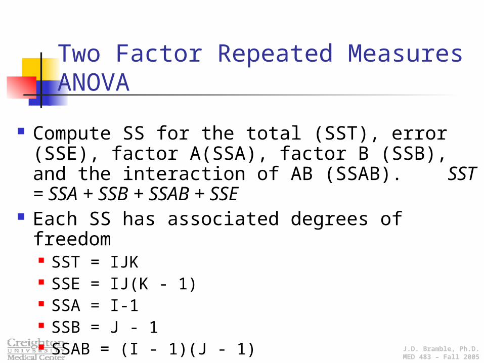
Compute SS for the total (SST), error (SSE), factor A(SSA), factor B (SSB), and the interaction of AB (SSAB). SST = SSA + SSB + SSAB + SSE

Each SS has associated degrees of freedom SST = IJK SSE = IJ(K - 1) SSA = I-1 SSB = J - 1 SSAB = (I - 1)(J - 1)

Two Factor Repeated Measures ANOVA


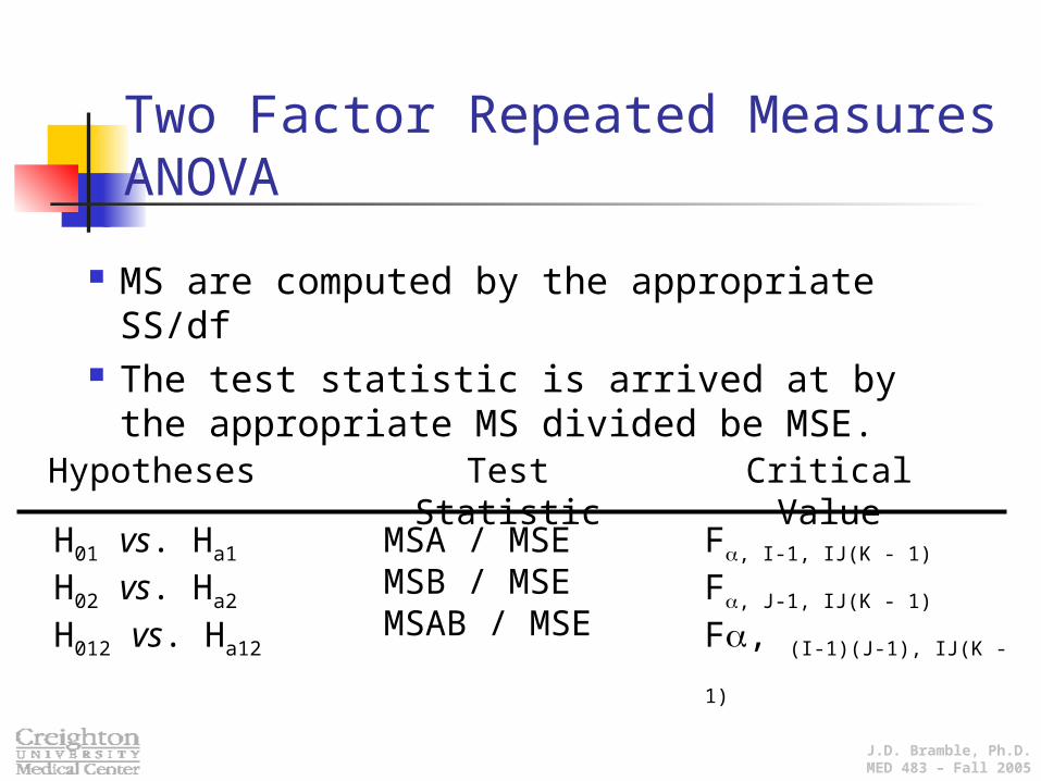
MS are computed by the appropriate SS/df The test statistic is arrived at by the

appropriate MS divided be MSE.

H01 vs. Ha1 H02 vs. Ha2

H012 vs. Ha12

F, I-1, IJ(K - 1) F, J-1, IJ(K - 1)

F, (I-1)(J-1), IJ(K - 1)

MSA / MSE MSB / MSEMSAB / MSE

Hypotheses Test Statistic Critical Value

Two Factor Repeated Measures ANOVA


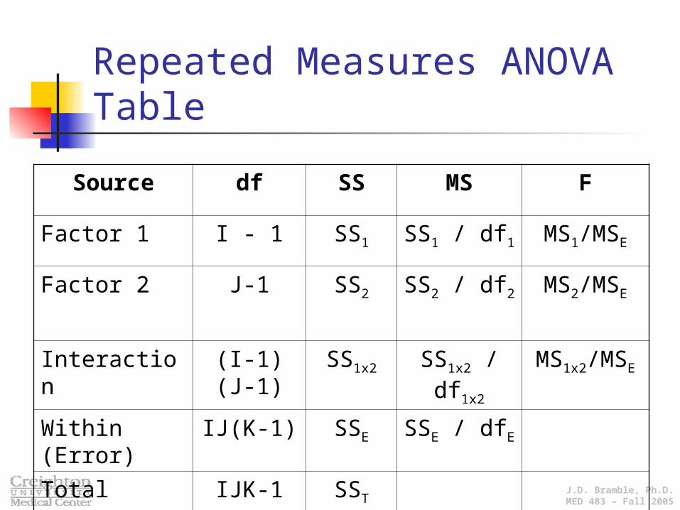
Repeated Measures ANOVA Table

Source df SS MS F

Factor 1 I - 1 SS1 SS1 / df1 MS1/MSE

Factor 2 J-1 SS2 SS2 / df2 MS2/MSE

Interaction (I-1)(J-1) SS1x2 SS1x2 / df1x2 MS1x2/MSE

Within (Error) IJ(K-1) SSE SSE / dfE

Total IJK-1 SST


The ANOVA Table

Source df SS MS F

Music 2 740 370 48.89

Stage 1 30 30 4.05

Music x Stage 2 260 130 17.53

Error 24 178 7.42

Total 29 1208


Repeated Measures: Tukey’s

When no significant interaction is found For comparing levels of factor A, obtain Q, I,

IJ(K - 1)

For comparing levels of factor B, obtain Q,

J, IJ(K - 1)

w = Q * MSE/JK for factor 1 comparisons

w = Q * MSE/IK for factor 2 comparisons Arrange sample means in increasing order and

underscore pairs of differing by less than w


Multivariate Analysis of Variance

Referred to as MANOVA Used when there is multiple dependent

variables Dependent variables are usually releted to

one another MANOVA helps to determine the effect of

the treatment (IV) on any one outcome (DV)


MANOVA Example Does sex, race, and educational level affect how well

people deal with the pressure of a terminal disease?

IV = sex (2), race (4), education (4)

DV = Coping strategies (5)

MANOVA can estimate the effects of the IV (sex, race, and education) for each of the five scales of coping strategies, independent of one another.


Analysis of Covariance Referred to as ANCOVA Allows researchers to adjust or equalize

baseline differences between groups In addition to the DV and IV a covariate is

enter into the model. The covariate is a variable that is known to

have an effect on the DV


ANCOVA example Wood et al. (2002) tested an educational intervention

to promote breast self examination (BSE).

Quasi experimental design

Difference in knowledge and skill related to BSE.

Enter these covariates into the model is essential to determine if the difference is the intervention or the initial difference

J.D. Bramble, Ph.D. Creighton University Medical Center Med 483 -- Fall 2005 Confidence Intervals.

Documents

Transcript of J.D. Bramble, Ph.D. Creighton University Medical Center Med 483 -- Fall 2005 Confidence Intervals.