January 2021 (last version before print)
47
January 2021 (last version before print) SALES AND MARKUP DISPERSION: THEORY AND EMPIRICS MONIKA MRÁZOVÁ Geneva School of Economics and Management, University of Geneva, CEPR, and CESifo J. PETER NEARY Department of Economics, University of Oxford, CEPR, and CESifo MATHIEU PARENTI ECARES, Universite Libre de Bruxelles and CEPR We characterize the relationship between the distributions of two variables linked by a structural model. We then show that, in models of heterogeneous firms in monopolistic com- petition, this relationship implies a new demand function that we call “CREMR” (Constant Revenue Elasticity of Marginal Revenue). This demand function is the only one that is con- sistent with productivity and sales distributions having the same form (whether Pareto, log- normal, or Fréchet) in the cross section, and it is necessary and sufficient for Gibrat’s Law to hold over time. Among the applications we consider, we use our methodology to characterize misallocation across firms; we derive the distribution of markups implied by any assumptions on demand and productivity; and we show empirically that CREMR-based markup distribu- tions provide an excellent parsimonious fit to Indian firm-level data, which in turn allows us to calculate the proportion of firms that are of sub-optimal size in the market equilibrium. KEYWORDS: CREMR Demands, Gibrat’s Law, Heterogeneous Firms, Lognormal versus Pareto Distributions, Sales and Markup Distributions. 1. INTRODUCTION THE HYPOTHESIS OF A REPRESENTATIVE AGENT has provided a useful starting point in many fields of economics. However, sooner or later, both intellectual curiosity and the exigencies of matching empirical evidence make it desirable to take account of agent heterogeneity. In many cases, this involves constructing models with three components. First is a distribution of agent characteristics, usually assumed exogenous; second is a model of individual agent behavior; and third, implied by the first two, is a predicted distribution of outcomes. Models of this kind are now pervasive in many research areas, including income distribution, optimal income tax- ation, macroeconomics, and urban economics. 1 In the field of international trade they have Monika Mrázová: [email protected] J. Peter Neary: [email protected] Mathieu Parenti: [email protected] This paper was first presented at ETSG 2014 in Munich under the title “Technology, Demand, and the Size Dis- tribution of Firms”. We are particularly grateful to Jan De Loecker and Julien Martin for assisting us with the data, to Stéphane Guerrier for computational advice, to the editor and five anonymous referees, to our conference discus- sants, Costas Arkolakis, Luca Macedoni, Marc Melitz, Gianmarco Ottaviano, Ina Simonovska, Frank Verboven, and Tianhao Wu, and also to Abi Adams, Andy Bernard, Bastien Chopard, Jonathan Dingel, Peter Egger, Xavier Gabaix, Basile Grassi, Arshia Hashemi, Joe Hirschberg, Oleg Itskhoki, Jérémy Lucchetti, Rosa Matzkin, Isabelle Méjean, David Preinerstorfer, Steve Redding, Kevin Roberts, Stefan Sperlich, Jens Südekum, Gonzague Vannoorenberghe, Maria-Pia Victoria-Feser, Frank Windmeijer, and participants at various conferences and seminars, for helpful com- ments and discussions. Monika Mrázová thanks the Fondation de Famille Sandoz for funding under the “Sandoz Family Foundation – Monique de Meuron” Programme for Academic Promotion. Peter Neary thanks the European Research Council for funding under the European Union’s Seventh Framework Programme (FP7/2007-2013), ERC grant agreement no. 295669. 1 For examples, see Stiglitz (1969), Mirrlees (1971), Krusell and Smith (1998), and Behrens et al. (2014), respec- tively.
Transcript of January 2021 (last version before print)

January 2021 (last version before print)
SALES AND MARKUP DISPERSION: THEORY AND EMPIRICS
MONIKA MRÁZOVÁGeneva School of Economics and Management, University of Geneva, CEPR, and CESifo
J. PETER NEARYDepartment of Economics, University of Oxford, CEPR, and CESifo
MATHIEU PARENTIECARES, Universite Libre de Bruxelles and CEPR
We characterize the relationship between the distributions of two variables linked by astructural model. We then show that, in models of heterogeneous firms in monopolistic com-petition, this relationship implies a new demand function that we call “CREMR” (ConstantRevenue Elasticity of Marginal Revenue). This demand function is the only one that is con-sistent with productivity and sales distributions having the same form (whether Pareto, log-normal, or Fréchet) in the cross section, and it is necessary and sufficient for Gibrat’s Law tohold over time. Among the applications we consider, we use our methodology to characterizemisallocation across firms; we derive the distribution of markups implied by any assumptionson demand and productivity; and we show empirically that CREMR-based markup distribu-tions provide an excellent parsimonious fit to Indian firm-level data, which in turn allows usto calculate the proportion of firms that are of sub-optimal size in the market equilibrium.
KEYWORDS: CREMR Demands, Gibrat’s Law, Heterogeneous Firms, Lognormal versusPareto Distributions, Sales and Markup Distributions.
1. INTRODUCTION
THE HYPOTHESIS OF A REPRESENTATIVE AGENT has provided a useful starting point in manyfields of economics. However, sooner or later, both intellectual curiosity and the exigencies ofmatching empirical evidence make it desirable to take account of agent heterogeneity. In manycases, this involves constructing models with three components. First is a distribution of agentcharacteristics, usually assumed exogenous; second is a model of individual agent behavior;and third, implied by the first two, is a predicted distribution of outcomes. Models of this kindare now pervasive in many research areas, including income distribution, optimal income tax-ation, macroeconomics, and urban economics.1 In the field of international trade they have
Monika Mrázová: [email protected]. Peter Neary: [email protected] Parenti: [email protected] paper was first presented at ETSG 2014 in Munich under the title “Technology, Demand, and the Size Dis-
tribution of Firms”. We are particularly grateful to Jan De Loecker and Julien Martin for assisting us with the data,to Stéphane Guerrier for computational advice, to the editor and five anonymous referees, to our conference discus-sants, Costas Arkolakis, Luca Macedoni, Marc Melitz, Gianmarco Ottaviano, Ina Simonovska, Frank Verboven, andTianhao Wu, and also to Abi Adams, Andy Bernard, Bastien Chopard, Jonathan Dingel, Peter Egger, Xavier Gabaix,Basile Grassi, Arshia Hashemi, Joe Hirschberg, Oleg Itskhoki, Jérémy Lucchetti, Rosa Matzkin, Isabelle Méjean,David Preinerstorfer, Steve Redding, Kevin Roberts, Stefan Sperlich, Jens Südekum, Gonzague Vannoorenberghe,Maria-Pia Victoria-Feser, Frank Windmeijer, and participants at various conferences and seminars, for helpful com-ments and discussions. Monika Mrázová thanks the Fondation de Famille Sandoz for funding under the “SandozFamily Foundation – Monique de Meuron” Programme for Academic Promotion. Peter Neary thanks the EuropeanResearch Council for funding under the European Union’s Seventh Framework Programme (FP7/2007-2013), ERCgrant agreement no. 295669.
1For examples, see Stiglitz (1969), Mirrlees (1971), Krusell and Smith (1998), and Behrens et al. (2014), respec-tively.

2
rapidly become the dominant paradigm, since the increasing availability of firm-level exportdata from the mid-1990s onwards undermined the credibility of representative-firm models,and stimulated new theoretical developments. A key contribution was Melitz (2003), who builton Hopenhayn (1992) to derive an equilibrium model of monopolistic competition with hetero-geneous firms. In this setting, the model structure combines assumptions about the distributionof firm productivity and about the form of demand that firms face, and from these derives pre-dictions about the distribution of firm sales. Such models have provided a fertile laboratory forstudying a wide range of problems relating to the process of globalization. However, with afew exceptions to be discussed below, we know little about how different assumptions aboutthe distributions of two variables and the structural model that links them are related to eachother.
In this paper we first provide a complete characterization of this problem in the general case.This reveals how a structural model constrains the choice of assumptions and the outcomesthat are consistent with them. We then show that, in models of heterogeneous firms in mo-nopolistic competition, this implies a new demand function that we call “CREMR” (ConstantRevenue Elasticity of Marginal Revenue). This demand function is the only one that is consis-tent with productivity and sales distributions having the same form (whether Pareto, lognormal,or Fréchet) in the cross section; and, with additive separability, it is necessary and sufficient forGibrat’s Law, a central result in the dynamics of firm size and industry structure, which pre-dicts that the growth rate of firm sales is independent of firm size. Among the applications weconsider, we use our methodology to characterize misallocation across firms; we derive thedistribution of markups implied by any assumptions on demand and productivity; and we showempirically that CREMR-based markup distributions provide an excellent parsimonious fit toIndian firm-level data, which in turn allows us to calculate the proportion of firms that are ofsub-optimal size in the market equilibrium.
Existing results in the theoretical literature on heterogeneous firms highlight important spe-cial cases in models of monopolistic competition, but give little guidance as to whether theinsights can be generalized. Helpman et al. (2004) and Chaney (2008) considered what can becalled the canonical model in this field, where firm productivities have a Pareto distributionand demands are CES. They showed that in this case the implied distribution of sales is alsoPareto. Head et al. (2014) derived a second result with a similar flavor: lognormal productivi-ties plus CES demands imply a lognormal distribution of firm sales. Finally, the literature onGibrat’s Law has shown that the rate of growth of a firm’s sales is independent of its size, fol-lowing both idiosyncratic and industry-wide productivity shocks in monopolistic competitionwith CES demands. (See Luttmer (2007, 2011), Arkolakis (2010a,b, 2016).)
All these results give sufficient conditions for the distribution of sales or sales growth to takea particular form. This leaves open the question of whether there are necessary conditions thatcan be stated, and in particular whether any demand functions other than CES are consistentwith results of this kind. CES demands have great analytic convenience: their tractability hasmade it possible to extend CES-based models to incorporate various real-world features of theglobal economy, such as outsourcing, multi-product firms, and global value chains.2 However,in a monopolistically competitive setting they also have strong counterfactual implications. Inparticular, they imply that markups are constant across space and time: in a cross section, allfirms should have the same markup in all markets; while, in time series, exogenous shockssuch as globalization cannot affect markups and so competition effects will never be observed.Trade economists have been uneasy with these stark predictions for some time, and a numberof contributions has explored the implications of relaxing the CES assumption, though to date
2See Antràs and Helpman (2004), Bernard et al. (2011), and Antràs and Chor (2013), respectively.

SALES AND MARKUP DISPERSION: THEORY AND EMPIRICS 3
without considering their implications for sales and markup distributions.3 Only recently has itbecome possible to confront the predictions of CES-based models with data, following the de-velopment of techniques for measuring markups that do not impose assumptions about marketstructure or the functional form of demand. In particular, De Loecker et al. (2016) show that thedistribution of markups from a sample of Indian firms is very far from being concentrated at asingle value. (We discuss their data in more detail in Section 6.1 below.) A possible explanationis that such markup heterogeneity arises from aggregation across sectors with different elastic-ities of substitution. However, Lamorgese et al. (2014), who use data on Chilean firms, showthat markup heterogeneity persists when the data are disaggregated by sector. Taken together,this evidence suggests that markup distributions are far from the Dirac form implied by CESdemands, but the literature to date has paid little attention to the form of these distributionsimplied by alternative assumptions and how well they match the data.
In addition to our substantive results, we make two technical contributions. First, we intro-duce the “Generalized Power Function” class of probability distributions. This nests many two-parameter distributions, including Pareto, lognormal and Fréchet, and allows compact proofsthat apply to all these cases. Second, we introduce the property of “h-reflection” of two distri-butions: the distribution of z is a h-reflection of that of y if the distributions of y and h(z) aremembers of the same family of distributions, where h(z) is a monotonically increasing func-tion. This provides a unifying principle for a range of new results relating the distributions offirm characteristics and the economic model that links them.
The rest of the paper proceeds as follows. Section 2 states a general proposition which char-acterizes the form that distributions of agent characteristics and models of agent behavior musttake if they are to be mutually consistent. Section 3 applies this result in the context of hetero-geneous firms in monopolistic competition to characterize the links between the distributions offirm productivity and firm sales, and the structure of demand. This Section highlights our newCREMR demand function, and explores its properties. Sections 4 and 5 apply these results todistributions of output (in both the market equilibrium and the social optimum), and markups,respectively. Section 6 provides a quantitative illustration of various theoretical results fromprevious sections. First, we take to data a selection of markup distributions implied by differ-ent assumptions about demand and the distribution of firm productivities. Out of the selectedalternatives, CREMR demands perform the best. We then use this best-fitting specification toquantify the degree of misallocation in a novel way. Finally, Section 7 concludes, while theAppendix and Online Appendix give proofs of propositions as well as further technical detailsand robustness checks.
2. CHARACTERIZING LINKS BETWEEN DISTRIBUTIONS
The first main result of the paper links the distributions of two agent characteristics to ageneral specification of the relationship between them: until Section 3 we make no assump-tions about whether either characteristic is exogenous or endogenous, nor about the underlyingstructural model that relates them. We assume a hypothetical dataset of a continuum of agents,which reports for each agent i its characteristics y(i) and z(i), both of which are monotonicallyincreasing functions of i.4 Formally:
3The implications of demand functions other than CES have been considered by Melitz and Ottaviano (2008),Zhelobodko et al. (2012), Fabinger and Weyl (2012), Bertoletti and Epifani (2014), Simonovska (2015), Feenstraand Weinstein (2017), Mrázová and Neary (2017), Parenti et al. (2017), Arkolakis et al. (2018), and Feenstra (2018),among others.
4Conditional on monotonicity, the assumption that y(i) and z(i) are increasing in i is without loss of generality.For example, if y(i) is increasing and z(i) is decreasing, Proposition 1 can easily be reformulated using the survival

4
ASSUMPTION 1: i, y(i), z(i) ∈Ω×R2+, where Ω is the set of agents, with both y(i) and
z(i) monotonically increasing functions of i.
Examples of y(i) and z(i) in models of heterogeneous firms include productivity, sales andmarkups.
In addition, we assume that the distributions of the two agent characteristics share a commonparametric structure:
DEFINITION 1: A family of probability distributions is a member of the “Generalized PowerFunction” (GPF) class of distributions if there exists a continuously differentiable functionH(·) such that the cumulative distribution function of every member of the family can bewritten as:
G (y;θ) =H
(θ0 +
θ1
θ2
yθ2)
(1)
where each member of the family corresponds to a particular value of the vector θ ≡θ0, θ1, θ2.
The function H(·) is completely general, other than exhibiting the minimal requirements of aprobability distribution: G(y;θ) = 0 and G(y;θ) = 1, where [y, y] is the support of G; and, tobe consistent with a strictly positive density function, Gy > 0, H(·) must satisfy the restriction:θ1H
′ > 0. As we show in Appendix A.1, the great convenience of the GPF class given by (1)is that it nests many of the most widely-used families of distributions in applied economics,including Pareto, lognormal, uniform, Fréchet, Weibull, and Gumbel, as well as their truncatedversions.
Given Assumption 1 and Definition 1, we can now state our main result:
PROPOSITION 1: Assume Assumption 1 holds. Then any two of the following imply the third:(A) The distribution of y is a member of the GPF class:
G(y;θ) =H
(θ0 +
θ1
θ2
yθ2), Gy > 0
(B) The distribution of a monotonically increasing function of z, h(z), h′ > 0, is a member ofthe same family of distributions as that of y but with different values of θ1 and θ2:
F (z;θ′) =G (h(z);θ′) =H
(θ0 +
θ′1θ′2h(z)θ
′2
), Fz > 0
(C) y is a power function of h(z): y = y0h(z)E;where the parameters are related as follows:
(i) (A) and (C) imply (B) with θ′1 = Eθ1yθ20 and θ′2 = Eθ2; similarly, (B) and (C) imply (A)
with θ1 =E−1θ′1y−E−1θ′20 and θ2 =E−1θ′2.
function of z. By contrast, the assumption that they are monotonic in i is an important restriction, though one thatis satisfied by most firm characteristics in models with uni-dimensional firm heterogeneity, on which we focus here.(For models with multi-dimensional heterogeneity, see Hallak and Sivadasan (2013), Holmes and Stevens (2014),and Harrigan and Reshef (2015).) Note that we require that monotonicity hold in theoretical models only: measuredfirm characteristics need not be monotonically related in the data.

SALES AND MARKUP DISPERSION: THEORY AND EMPIRICS 5
(ii) (A) and (B) imply (C) with y0 =(θ2θ1
θ′1θ′2
) 1θ2 and E =
θ′2θ2
.
The proof is in Appendix A.2. Comparing the distributions of y and h(z) in (A) and (B), theyare members of the same family of the GPF class, except that the parameter vectors θ and θ′
are different. The h(·) function is completely general, except that it must be monotonically in-creasing from the monotonicity restriction on F : h′ > 0 since Fz =Gyh
′ > 0; and the elementsof θ can take on any values, except that θ0 must be the same for both distributions.
Each choice of the h(·) function generates in turn a further family, such that the transforma-tion h(z) follows a distribution from the GPF class. Proposition 1 shows that these families areintimately linked via a simple power function that expresses one of the two agent characteris-tics as a transformation of the other. We say that the distribution of z is a h-reflection of that ofy:5
DEFINITION 2: The distribution of z is a h-reflection of the distribution of y if the distribu-tions of y and h(z) are members of the same family of distributions.
In the remainder of the paper, we apply Proposition 1 to the setting of heterogeneous firms inmonopolistic competition. Our theoretical results can be categorized by the type of h-reflectionthey exhibit. One central case is where h(z) is the identity transformation, h(z) = z. We callthis case “self-reflection”, since it implies from Proposition 1 that the distributions of y andz are members of the same family. This case proves particularly useful when we considerdistributions of firm sales and the rate of growth of firm sales in Section 3.
When we come to consider the distributions of output in the market equilibrium and thesocial optimum in Section 4, we will see that they exhibit “marginal-revenue reflection” and“marginal-utility reflection” of the distribution of productivity respectively. Finally, when wecome to consider the distributions of sales and firm markups for a range of demand functions inSection 5, we will see that they exhibit a wide range of forms for the h function. One importantcase is the odds transformation, h(z) = z
1−z , where 0≤ z ≤ 1. When the distributions of y andof an odds transformation of z are members of the same family, we say that the distribution ofz exhibits “odds reflection” of that of y. This case proves particularly useful when we considerdistributions of firm markups.
3. SELF-REFLECTION OF PRODUCTIVITY AND SALES: CREMR DEMANDS
In this section we explore some implications of Proposition 1 in models of monopolisticcompetition with heterogeneous firms and general demands. In particular, we ask what demandfunctions are consistent with the distributions of firm productivity and sales revenue exhibitingself-reflection, so the two distributions are members of the same family from the GPF classthough with different parameters. (Appendix A.4 gives related results for self-reflection of pro-ductivity and output and of sales and output.) As noted in the introduction, there are only tworesults in the literature that relate productivity and sales distributions: Helpman et al. (2004)and Chaney (2008) showed that CES demands are sufficient to bridge the gap between twoPareto distributions; and Head et al. (2014) showed that the same holds for two lognormaldistributions. Given the abundant empirical evidence that both firm productivity and sales are
5The property of h-reflection is not symmetric in general: the fact that the distribution of z is a h-reflection of thedistribution of y does not imply that the distribution of y is a h-reflection of the distribution of z. Also h-reflectionis not in itself related to the GPF class, though all the cases we consider in the paper assume that the distributions ofboth y and h(z) are members of a family of the GPF class.

6
either Pareto or lognormal shaped, self-reflection is a natural starting point in trying to gen-eralize these results.6 Our results illustrate the power of Proposition 1: it leads to a completecharacterization of the conditions under which self-reflection holds. This yields a new demandfunction that we call “CREMR”, which implies functional forms for the distribution of markupsfor which we find strong evidence in our empirical section. In Section 3.3, we give a furthermotivation for self-reflection, showing that it is central to an important substantive question:when does Gibrat’s Law hold in monopolistic competition? We show that, under additive sep-arability, self-reflection of cumulated productivity shocks and sales growth rates over time isequivalent to Gibrat’s Law, so Proposition 1 implies that CREMR demands are necessary andsufficient for this Law to hold in a monopolistically competitive industry. Given these importantimplications of CREMR demands, it is desirable to understand their properties and to considerwhat preferences rationalize them: Sections 3.4 and 3.5 consider these topics respectively.
We begin in Section 3.1 by introducing the monopolistically competitive setting we will usein the remainder of the paper.
3.1. The Monopolistically Competitive Setting
Consider a model of a monopolistically competitive industry with heterogeneous firms inthe tradition of Melitz (2003), extended to allow for non-CES demands. Firms differ in theirproductivity, ϕ, which is drawn from an underlying distribution G(ϕ) with support [ϕmin,∞)upon paying a sunk entry cost fe. They incur a common fixed cost f which may be zero inthe case when the demand function implies a finite upper bound for marginal revenue. Eachfirm produces a unique good, and chooses its output x to maximize its profits π, which equaloperating profits less fixed costs:
π(ϕ,λ, τ) = maxx
((p(x,λ)− τϕ−1
)x− f
)(2)
Here, p(x,λ) is the inverse demand function of a representative consumer faced by all firms,which depends negatively on their output level x and on λ, a common demand parameter thatis exogenous to firms but endogenous to the industry. From each firm’s perspective, λ is ameasure of the intensity of competition which it takes as given.7 Finally, τ is a uniform costshifter that is common to all firms; until Section 3.3 we set this equal to one.
Maximizing profits as in (2) leads to the first-order condition, which equates marginal rev-enue to marginal cost:
p(x,λ) + xpx(x,λ) = ϕ−1 (3)
Assuming the second-order condition 2px(x,λ) + xpxx(x,λ)< 0 is satisfied, (3) implies thatthe equilibrium output and price of each firm are functions of its productivity ϕ and of thedemand shifter λ, where the latter is the same for all firms. In Section 3.2, we suppress λ tosimplify notation. In the rest of the paper, we denote by G (ϕ) the distribution of operating
6Axtell (2001) and Gabaix (2009) argue that the distribution of firm sales is plausibly close to Pareto, at least inthe upper tail. However, Head et al. (2014) and Bee and Schiavo (2018) argue that it is better approximated overallby a lognormal, and Fernandes et al. (2018) find that the intensive margin of firm sales is inconsistent with a Paretoproductivity distribution. We return to this issue in Online Appendix B.4.
7The specification of demand in (2) corresponds to the generalized separability class of Pollak (1972). It allowsfor various preference systems including additive separability as in Zhelobodko et al. (2012), Bertoletti and Epifani(2014), and Mrázová and Neary (2017). Results in Section 3.2 take a “firm’s-eye" view perspective and do not dependon the micro-foundation of demand. In Section 3.3 by contrast, we invoke additive separability when discussinggeneral-equilibrium effects.

SALES AND MARKUP DISPERSION: THEORY AND EMPIRICS 7
firms with support [ϕ,∞) where ϕ is the productivity of a cutoff firm that makes zero profitsin the market equilibrium.
3.2. Self-Reflection in the Cross Section: Productivity and Sales
The necessary condition for self-reflection follows immediately from Proposition 1: if thedistributions of productivity ϕ and sales r are from the same family, which can be any memberof the GPF class, then they must be related by a power function:
ϕ= ϕ0rE (4)
To infer the implications of this for demand, we use two properties of a monopolisticallycompetitive equilibrium. First, firms equate marginal cost to marginal revenue, so from (3)ϕ = c−1 =
(∂r∂x
)−1. Second, all firms face the same residual demand function, so firm salesconditional on output are independent of productivity ϕ: r(x) = xp(x) and ∂r
∂x= r′(x).8 Com-
bining these with (4) gives a simple differential equation in sales revenue:
(r′(x))−1 = ϕ0r(x)E (5)
Integrating this we find that a necessary and sufficient condition for self-reflection of produc-tivity and sales is that the inverse demand function takes the following form:
p(x) =β
x(x− γ)
σ−1σ , 1< σ <∞, x > γσ, β > 0 (6)
Calculating marginal revenue and inverting it brings us back to (4), with the constants ϕ0 andE equal to β−
σσ−1 σ
σ−1and 1
σ−1respectively.
We are not aware of any previous discussion of the family of inverse demand functions in(6), which express expenditure r(x) = xp(x) as a power function of consumption relative to abenchmark γ. Its key property, from (5), is that the elasticity of marginal revenue with respectto total revenue is constant: E = 1
σ−1. Hence we call it the “CREMR” family, for “Constant
Revenue Elasticity of Marginal Revenue.” Summarizing:
PROPOSITION 2: The distributions of firm productivity and firm sales revenue in modelsof monopolistic competition with heterogeneous firms are members of the same family of theGeneralized Power Function class if and only if demands take the CREMR form (6).
CREMR demands include CES demands as a special case: when γ equals zero, (6) reducesto p(x) = βx−
1σ , and the elasticity of demand is constant, equal to σ. More generally, the
elasticity of demand varies with consumption, ε(x)≡− p(x)
xp′(x)= x−γ
x−γσσ, though it approachesσ for large firms.9
It is useful to consider the implications of CREMR demands combined with Pareto andlognormal distributions of productivity. Starting with the Pareto, it follows immediately as acorollary of Proposition 1 that CREMR demands are necessary and sufficient for self-reflection
8Our approach is consistent with marginal costs being chosen endogenously by firms, either by optimizing subjectto a variable cost function, as in Zhelobodko et al. (2012), or as the outcome of investment in R&D, as in Bustos(2011). However, it is not in general consistent with oligopoly, as firms may face different residual demand functions.
9Note that this contrasts with CES models under oligopolistic competition (Atkeson and Burstein (2008)) wherethe price-elasticity of demand is equal to σ for the smallest firms only.

8
in this case. We state the result formally for completeness, and because it makes explicit thelinks that must hold between the parameters of the two Pareto distributions and the demandfunction.
COROLLARY 1: Given Assumption 1, any two of the following imply the third:(A) The distribution of firm productivity is Pareto: GP(ϕ) = 1−ϕkϕ−k;(B) The distribution of firm sales revenue is Pareto: FP(r) = 1− rnr−n;(C) The demand function belongs to the CREMR family in (6);where the parameters are related as follows:
n=k
σ− 1and r = βσ
(σ− 1
σϕ
)σ−1
This extends a result of Chaney (2008), who showed that n= kσ−1
with Pareto productivity andCES demands.
Turning next to the lognormal, since it is also a member of the GPF class, it follows imme-diately from Proposition 1 that the CREMR relationship ϕ= ϕ0r
E is necessary and sufficientfor self-reflection in the lognormal case. A complication is that, except in the CES case (whenthe CREMR parameter γ is zero), the value of sales revenue for the smallest firm is strictlypositive, whereas the lower bound of the lognormal distribution is zero.10 However, this is nota problem since, as we show in Corollary 3 in Appendix A.1, a truncated distribution from theGPF family is itself a member of the family. Hence we have the result (where Φ denotes thecumulative distribution function of the standard normal distribution and T denotes the fractionof potential firms that are inactive):
COROLLARY 2: Given Assumption 1, any two of the following imply the third:(A) The distribution of firm productivity is truncated lognormal with support [ϕ,+∞):GtLN (ϕ) = Φ((logϕ−µ)/s)−T
1−T ;(B) The distribution of firm sales revenue is truncated lognormal with support [r,+∞):
FtLN (r) =Φ((log r−µ′)/s′)−T
1−T ;(C) The demand function belongs to the CREMR family in (6);where the parameters are related as follows:
s′ = (σ− 1)s
µ′ = (σ− 1)
(µ+ log
(σ− 1
σβ
σσ−1
))
r =
(σ− 1
σβ
σσ−1ϕ
)σ−1
T = Φ((logϕ− µ)/s) = Φ ((log r− µ′)/s′)
10Since p′(x) =− β
σx2 (x− γ)−1σ (x− γσ), the output of the smallest active firm when γ is strictly positive is
greater than or equal to γσ, while its sales revenue is r(x) = β (γ(σ− 1))σ−1σ > 0. When γ is strictly negative,
sales revenue is discontinuous at x= 0: limx→0+
r(x) = β(−γ)σ−1σ > 0, but r(0) = 0.

SALES AND MARKUP DISPERSION: THEORY AND EMPIRICS 9
Just as in the Pareto case, CREMR is the only demand function that is compatible with lognor-mal productivity and sales.
We will see in Section 6 how these theoretical results translate to data.
3.3. Self-Reflection over Time: Gibrat’s Law
Having derived the necessary and sufficient conditions for self-reflection in the cross-section,we now turn to self-reflection over time. Specifically, we show that CREMR demands are nec-essary and sufficient for Gibrat’s Law, or “The Law of Proportionate Effect”, which assertsthat the rate of growth of a firm is independent of its size. There is persuasive empirical evi-dence in favor of the Law in general, especially for larger and older firms; see, for example,Haltiwanger et al. (2013). A variety of mechanisms has been proposed to explain this empiricalregularity.11 Early contributions, by Gibrat (1931) himself and by Ijiri and Simon (1974), gavepurely stochastic explanations. In particular, if firms are subject to i.i.d. idiosyncratic shocks,these cumulate to give an asymptotic lognormal distribution of firm size, all growing at thesame rate. Later work has shown how Gibrat’s Law can be derived as an implication of indus-try equilibrium, when firms are subject to industry-wide as well as idiosyncratic shocks. Muchof this work has been carried out under perfectly competitive assumptions, focusing on learn-ing, as in Jovanovic (1982), or differential access to credit, as in Cabral and Mata (2003). Theresult has also been shown to hold in models of monopolistic competition by Luttmer (2007,2011) and Arkolakis (2010a,b, 2016). However, these papers assume CES demand. Putting thisdifferently, all models that generate Gibrat’s Law to date imply that prices are either equal toor proportional to marginal costs. This raises the question whether Gibrat’s Law is consistentwith demand functions that allow for variable markups. The following proposition shows thatthis is indeed the case with CREMR demands:
PROPOSITION 3: In monopolistic competition with additive separability, CREMR demandsare necessary and sufficient for Gibrat’s Law to hold following: (i) industry-wide shocks to firmproductivity; and (ii) i.i.d. or AR(1) shocks to firm productivity.
Assume that the productivity process for firm i can be written as: ϕit = γitϕt, where ϕt is anindustry-wide shock, common to all firms, whereas γit is a firm-specific idiosyncratic shock.To prove Proposition 3, we consider each of these types of shocks in turn.
Consider first an industry-wide productivity shock, as in part (i). Intuitively, it is easy to seethat CREMR demands are necessary and sufficient for such a shock to have the same pro-portionate effect on the sales of all firms. This outcome is equivalent to a constant elasticityof sales revenue with respect to marginal cost (which is the inverse of productivity). Sincemarginal cost equals marginal revenue, this in turn is equivalent to the CREMR condition forself-reflection that we have already considered, which entails a constant elasticity of marginalrevenue with respect to total revenue; though the two conditions arise in different contexts:“cross-section” comparisons across firms in the case of self-reflection, “time-series” compar-isons between the pre- and post-productivity-shock equilibria in the case of Gibrat’s Law. Thissuggests that CREMR demands are necessary and sufficient for Gibrat’s Law to hold following
11For surveys of a large literature, see Sutton (1997) and Luttmer (2010). Gibrat’s Law has also been applied to thegrowth rate of cities. See, for example, Eeckhout (2004). We do not pursue this application here, but it is clear thatanalogous results to ours can be derived in that case. As Sutton (1997) points out, different authors have consideredshocks to either sales, employment, or assets. In a monopolistically competitive setting, it is natural to assume shocksto productivity, as below.

10
industry-wide shocks to firm productivity. We can show that this holds in general equilibriumwith additive separability.
Consider a uniform improvement in the productivity of all firms that we assume is exogenousand unanticipated: τ < 0 (where a circumflex denotes a logarithmic derivative: τ = d log τ , τ >0). The growth rate of sales following such a uniform productivity shock is: g ≡ − r
τ=− τ
rdrdτ
.Hence Gibrat’s Law ( dg
dϕ= 0) obtains when r is independent of ϕ.
We first consider the effects of the shock on each firm’s price and output. Starting with thehousehold’s first-order condition under additively separable preferences, p(x,λ) = λ−1u′(x)where u(·) denotes consumer’s sub-utility, totally differentiate to get the proportional changein prices:
p=−1
εx− λ
Hence the change in sales revenue is:
r = p+ x=ε− 1
εx− λ (7)
To solve for the proportional change in outputs we totally differentiate the firm’s first-ordercondition, (3):
x=−ε− 1
2− ρ(τ + λ), (8)
where ρ(x)≡−xp′′(x)
p′(x)is the convexity of the demand function. Finally, we substitute (8) into
(7), to obtain the change in sales revenue in terms of the cost shock τ and the implied changein the intensity of competition λ:
r =− (ε− 1)2
ε(2− ρ)︸ ︷︷ ︸(?)
(τ + λ)− λ
The way in which the change in the intensity of competition λ depends on the cost shockτ follows from the assumptions we make about market equilibrium: in particular, it differsbetween the cases of free entry and a fixed number of firms. Fortunately, these differences donot matter for our purposes, since in both cases τ and λ are the same for all firms. It followsthat a necessary and sufficient condition for Gibrat’s Law in this setting is that (?) is constantacross firms. This term, (ε−1)2
ε(2−ρ) , is the elasticity of revenue with respect to productivity. It isthe inverse of the elasticity of marginal revenue with respect to total revenue, which as wehave seen is constant if and only if demands are CREMR, in which case it equals 1
σ−1. (See
Section 3.2, and equation (32) in Appendix A.3.) This confirms that dg
dϕ= 0, i.e., with additive
separability, Gibrat’s Law holds following an industry-wide productivity shock in monopolisticcompetition, if and only if demands are CREMR.
To prove part (ii) of Proposition 3, consider now idiosyncratic shocks to firms’ productivity,which can be written as follows:
γit = γi,t−1eεit (9)

SALES AND MARKUP DISPERSION: THEORY AND EMPIRICS 11
where εit are identically distributed shocks with zero mean and finite variance. Equation (9)implies:
logϕit = logγ0t +t∑
t′=0
εit′ + logϕt
We consider the case of a stationary AR(1) growth rate without drift.12 Specifically, we allowfirm growth rates to be serially correlated:
εit = ξεi,t−1 + νit
where ξ < 1 and νit is white noise with constant variance υ2. (The special case of i.i.d. growthrates is readily obtained for ξ = 0 and νit i.i.d.) Then, as t→∞, and provided logγ0t + logϕtis small relative to logϕit, the distribution of ϕit is asymptotically lognormal:
logϕitt∼N
(0,
υ2
1− ξ2
)(10)
More generally, growth rate shocks will cumulate to give an asymptotic lognormal distributionif they admit a MA(∞) representation with absolutely summable coefficients. (See Hayashi(2000), Chapter 6, for extensions of the central limit theorem.) The final step is to recall thatproductivity equals the inverse of marginal revenue:
ϕit = ϕiγit = c−1it = (r′it)
−1
Now, we can invoke Proposition 2 and conclude that CREMR demands are necessary andsufficient for i.i.d. or AR(1) shocks to productivity to cumulate to give an asymptotic lognormaldistribution of sales, with firm growth rates independent of size. Note that Proposition 2 appliesin the cross-section. In the time series, idiosyncratic shocks also imply changes in λ hence thelevel of demand over time. As shown previously however, additive separability implies thatthese general equilibrium effects impact all firms proportionally, so that our cross-sectionalcharacterization still applies.
This completes the proof of Proposition 3: CREMR demands are necessary and sufficientfor Gibrat’s Law to hold in monopolistic competition with additive separability following bothidiosyncratic and industry-wide shocks to firm productivity.
A qualification that must be made is that the above micro-foundation of Gibrat’s law implies anon-stationary distribution of firm productivity and sales. Indeed, the asymptotic law expressedin (10) features a variance that increases quadratically with t. This creates a tension with theassumption that t must be large enough for the lognormal approximation to hold. This is awell-known problem which may be solved by adding a constant term to (9), see for instanceGabaix (1999) and Head et al. (2014). This yields a Kesten process which leads asymptoticallyto a Pareto distribution of productivities in the upper tail. Proposition 2 implies in this case thatCREMR is not necessary but still sufficient to obtain a Pareto distribution of sales in the uppertail.
3.4. Properties of CREMR Demands
Consider next the properties of the CREMR demand function (6). They are derived formallyin Appendix A.3, but can be understood by referring to the three sub-panels of Figure 1. These
12As long as drifts are not firm-specific, this assumption is made without loss of generality since industry-specificdrifts are captured by ϕt.

12
(a) γ = 0: CES (b) γ > 0: Subconvex (c) γ < 0: Superconvex
FIGURE 1.—Examples of CREMR demand and marginal revenue functions. Panels (a), (b), and (c) depict theCREMR demand from (6) (solid blue line) and marginal revenue from (29) (dotted orange line) for β = 1, σ = 1.4,and for γ equal to 0, 1 and −1 respectively.
show three representative inverse demand curves from the CREMR family, along with theircorresponding marginal revenue curves. The CES case in panel (a) combines the familiar ad-vantage of analytic tractability with the equally familiar disadvantage of imposing strong andcounter-factual properties. In particular, the markup m ≡ p
cmust be the same, equal to σ
σ−1,
for all firms in all markets. By contrast, members of the CREMR family with non-zero valuesof γ avoid this restriction. Moreover, we show in Appendix A.3 that the sign of γ determineswhether a CREMR demand function is more or less convex than a CES demand function. Thecase of a positive γ as in panel (b) corresponds to demands that are “subconvex”: less convexat each point than a CES demand function with the same elasticity. (See Mrázová and Neary(2019) for further discussion.) In this case the elasticity of demand falls with output, whichimplies that larger firms have higher markups. These properties are reversed when γ is nega-tive as in panel (c). Now the demands are “superconvex” – more convex than a CES demandfunction with the same elasticity – and larger firms have smaller markups. CREMR demandsthus allow for a much wider range of comparative statics responses than the CES itself. How
(a) CREMR Demands (b) Some Well-Known Demand Functions
FIGURE 2.—Demand manifolds for CREMR and other demand functions. Each curve shows the combinations ofelasticity ε and convexity ρ implied by the demand function indicated. Values of ε and ρ in the shaded region areinadmissible. See text for details.
do CREMR demands compare with other better-known demand systems? Inspecting the de-mand functions themselves is not so informative, as they depend on three different parameters.
SALES AND MARKUP DISPERSION: THEORY AND EMPIRICS 13
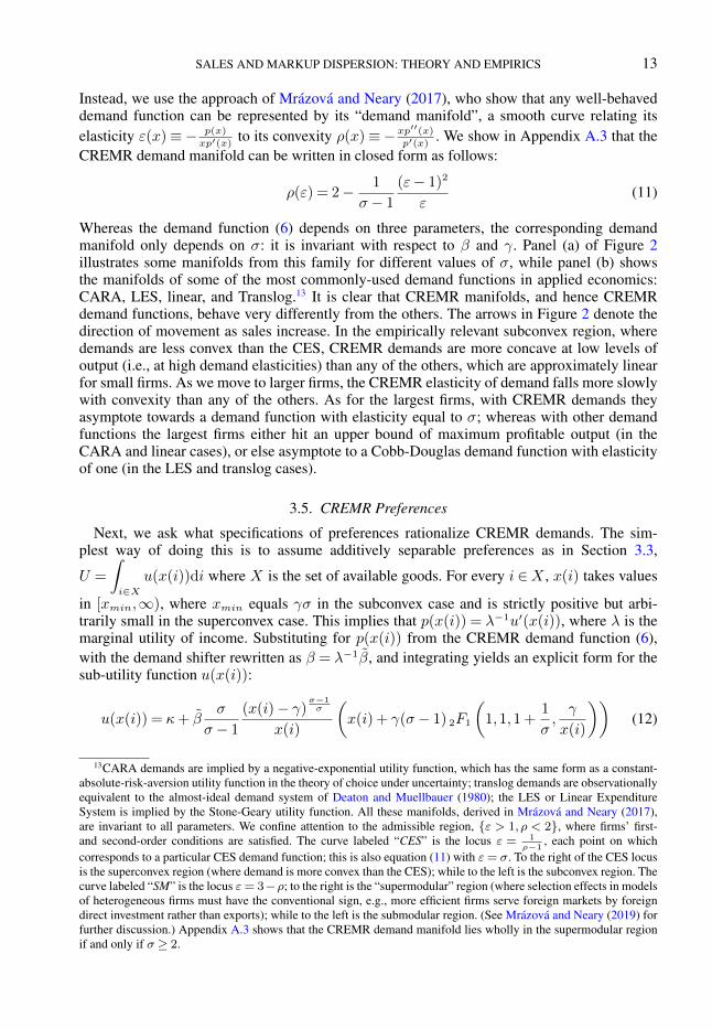
Instead, we use the approach of Mrázová and Neary (2017), who show that any well-behaveddemand function can be represented by its “demand manifold”, a smooth curve relating itselasticity ε(x)≡− p(x)
xp′(x)to its convexity ρ(x)≡−xp′′(x)
p′(x). We show in Appendix A.3 that the
CREMR demand manifold can be written in closed form as follows:
ρ(ε) = 2− 1
σ− 1
(ε− 1)2
ε(11)
Whereas the demand function (6) depends on three parameters, the corresponding demandmanifold only depends on σ: it is invariant with respect to β and γ. Panel (a) of Figure 2illustrates some manifolds from this family for different values of σ, while panel (b) showsthe manifolds of some of the most commonly-used demand functions in applied economics:CARA, LES, linear, and Translog.13 It is clear that CREMR manifolds, and hence CREMRdemand functions, behave very differently from the others. The arrows in Figure 2 denote thedirection of movement as sales increase. In the empirically relevant subconvex region, wheredemands are less convex than the CES, CREMR demands are more concave at low levels ofoutput (i.e., at high demand elasticities) than any of the others, which are approximately linearfor small firms. As we move to larger firms, the CREMR elasticity of demand falls more slowlywith convexity than any of the others. As for the largest firms, with CREMR demands theyasymptote towards a demand function with elasticity equal to σ; whereas with other demandfunctions the largest firms either hit an upper bound of maximum profitable output (in theCARA and linear cases), or else asymptote to a Cobb-Douglas demand function with elasticityof one (in the LES and translog cases).
3.5. CREMR Preferences
Next, we ask what specifications of preferences rationalize CREMR demands. The sim-plest way of doing this is to assume additively separable preferences as in Section 3.3,
U =
∫i∈X
u(x(i))di where X is the set of available goods. For every i ∈X , x(i) takes values
in [xmin,∞), where xmin equals γσ in the subconvex case and is strictly positive but arbi-trarily small in the superconvex case. This implies that p(x(i)) = λ−1u′(x(i)), where λ is themarginal utility of income. Substituting for p(x(i)) from the CREMR demand function (6),with the demand shifter rewritten as β = λ−1β, and integrating yields an explicit form for thesub-utility function u(x(i)):
u(x(i)) = κ+ βσ
σ− 1
(x(i)− γ)σ−1σ
x(i)
(x(i) + γ(σ− 1) 2F1
(1,1,1 +
1
σ,γ
x(i)
))(12)
13CARA demands are implied by a negative-exponential utility function, which has the same form as a constant-absolute-risk-aversion utility function in the theory of choice under uncertainty; translog demands are observationallyequivalent to the almost-ideal demand system of Deaton and Muellbauer (1980); the LES or Linear ExpenditureSystem is implied by the Stone-Geary utility function. All these manifolds, derived in Mrázová and Neary (2017),are invariant to all parameters. We confine attention to the admissible region, ε > 1, ρ < 2, where firms’ first-and second-order conditions are satisfied. The curve labeled “CES” is the locus ε = 1
ρ−1, each point on which
corresponds to a particular CES demand function; this is also equation (11) with ε= σ. To the right of the CES locusis the superconvex region (where demand is more convex than the CES); while to the left is the subconvex region. Thecurve labeled “SM” is the locus ε= 3−ρ; to the right is the “supermodular” region (where selection effects in modelsof heterogeneous firms must have the conventional sign, e.g., more efficient firms serve foreign markets by foreigndirect investment rather than exports); while to the left is the submodular region. (See Mrázová and Neary (2019) forfurther discussion.) Appendix A.3 shows that the CREMR demand manifold lies wholly in the supermodular regionif and only if σ ≥ 2.

14
This equals a constant of integration κ plus a primitive preference parameter β times the prod-uct of two functions, one an augmented CES, the other an augmented hypergeometric:
2F1(a, b; c;z) =∞∑n=0
(a)n (b)n(c)n
zn
n!, |z|< 1, (q)n =
Γ(q+ n)
Γ(q)(13)
where (q)n is the (rising) Pochhammer symbol, and Γ(q) is the gamma function. The onlydemand parameter that varies with income and other prices is β; it depends on λ, whose valuecan be recovered in a standard way.14 When γ is zero, the hypergeometric function also equals
(a) γ = 0: CES (b) γ > 0 (c) γ < 0
FIGURE 3.—Examples of CREMR sub-utility functions. Each panel shows the values of sub-utility u implied by(12) as a function of x for the same parameter values as in Figure 1: β = 1, σ = 1.4, and γ equal to 0, 1 and −1 inpanels (a), (b), and (c) respectively.
zero, and so (12) reduces to the CES utility function, u(x(i)) = β σσ−1
x(i)σ−1σ + κ. Figure
3 illustrates three sub-utility functions from the CREMR family, each as a function of x, fordifferent values of γ. Panel (a) is the CES case, showing that utility is increasing and concavein x. The subconvex case in Panel (b) and the superconvex case in Panel (c) (with positive andnegative values of γ respectively) deviate from the CES case in ways that parallel the ways thatthe corresponding demand functions differ from CES demands in Figure 1. In particular, utilityis defined on the same range as the demand function. If needed, they can both be extended inan appropriate way on the entire positive range to guarantee love for variety.
In some applications it may be desirable to have a homothetic specification of preferencesconsistent with CREMR demands. This is not possible with additive separability (which im-plies homotheticity only in the CES case), but it can be done by embedding CREMR de-mands in the implicitly additive preferences of Kimball (1995).15 Here the sub-functions cor-responding to each good depend on the consumption of that good scaled by total utility U :∫i∈X
Υ
(x(i)
U
)di= 1. Proceeding as in the additively separable case, we can combine the
first-order condition Υ′(x(i)
U
)= λp(i) with the CREMR demand function (6) and integrate,
14Inverting (6) yields the direct demand functions: x(i) = (u′)−1(λp(i)), which can be combined with the budgetconstraint to obtain:
∫i∈X p(i) (u′)−1(λp(i)) di = I (where I denotes consumer income). Solving this gives λ as
a function of prices and income. Note that x(i) cannot be written in closed form, but the marginal utility function isinvertible provided the elasticity of demand is positive, i.e., provided x(i) ∈ [xmin,∞).
15Fally (2018) shows that CREMR demands can be integrated to give utility functions from other members of thesingle-aggregate Pollak (1972) generalized separability class, but only in the superconvex case.

SALES AND MARKUP DISPERSION: THEORY AND EMPIRICS 15
which shows that the Υ sub-function takes the same form as u(x(i)) in (12).16 Unlike the morefamiliar Klenow and Willis (2016) special case of Kimball preferences, the Kimball-CREMRdirect utility and demand functions cannot be written in closed form, but they can still be usedas a foundation for quantitative analysis of normative issues.
4. MISALLOCATION ACROSS FIRMS
Section 3 used part (ii) of Proposition 1 to back out the demands implied by assumed dis-tributions of two firm characteristics. In this section and the next we show how part (i) of theProposition can be used to derive distributions of firm characteristics given the distribution ofproductivity and the form of the demand function. In this section we show how to compare thedistributions of output across firms in the market equilibrium and in the social optimum. Previ-ous comparisons between the allocation of resources in a monopolistically competitive marketand in the optimum that a social planner would choose have largely focused on the extensivemargin, addressing the question of whether the market leads to an under- or over-supply ofvarieties relative to the social optimum when preferences are additively separable. Dixit andStiglitz (1977) provided the definitive answer to this question when firms are homogeneous:the market is efficient, in the sense that it supplies the socially optimal number of varieties,and the optimal output of each, if and only if preferences are CES. Feenstra and Kee (2008)showed that the market is also efficient with CES preferences if firms are heterogeneous andthe distribution of firm productivities is Pareto, while Dhingra and Morrow (2019) present ageneral qualitative analysis of the heterogeneous-firm case. Here we focus on a quantitativecomparison between the market outcome and the optimal allocation at the intensive margin.In particular, we show in Section 4.1 how our methods from previous sections can be used toderive closed-form expressions for the distributions of output in the competitive market equi-librium and in the social optimum. In Section 4.2 we compare the two distributions explicitlyin the CREMR case, showing that, if and only if demand is subconvex, competitive marketsencourage too many small firms and not enough large ones relative to the optimum. Other au-thors have derived related results in different contexts: e.g., Nocco et al. (2014), Edmond et al.(2015), and Behrens et al. (2020). However, these take different approaches from ours; in par-ticular, they allow the extensive margin to adjust, and they do not compare the optimal andmarket output distributions directly as we do.
4.1. Equilibrium and Optimal Output Distributions
We wish to compare the market outcome with the social optimum. Consider first the former.Recalling from (3) that the first-order condition for each firm is that marginal cost should equalmarginal revenue, so the productivity-output relationship is:
ϕ(x) =1
r′(x)=
1
p(x) + xp′(x)(14)
16Now the direct demand functions depend on two aggregates rather than one, the true price index Pand the shadow price of the budget constraint λ: x(i) = (Υ′)−1 (λp(i)) I
P. To solve for these we use two
equations: first, the equation given in the text that implicitly defines U , evaluated at the optimal quantities:∫i∈XΥ ((Υ′)−1 (λp(i))) di= 1; and, second, the definition of the price index: P =
∫i∈Xp(i)(Υ
′)−1 (λp(i)) di.See Matsuyama and Ushchev (2017) for further details.

16
Letting G(ϕ) denote the productivity distribution of operating firms as before, (14) implies anew family of distributions, that we can call the “inverse marginal-revenue reflection” family:
J(x) =G(ϕ(x)) =G
(1
p(x) + xp′(x)
)(15)
Using (15), we can compute the distribution of firm output in the market equilibrium J(x) forany distribution of firm productivities G(ϕ) and any demand function p(x).
Consider next the social optimum. Following Dixit and Stiglitz (1977), we assume that thesocial planner cannot use lump-sum taxes or subsidies to affect profits. Extending the logic ofthis assumption to a heterogeneous-firms context, the feasible optimum is a constrained one,where the planner faces the same constraints as the market. In particular, she takes as given themass of entrants, Ne, and the productivity threshold, ϕ, equal to the productivity of a cutofffirm that makes zero profits in the market equilibrium. Given these, she maximizes aggregateutility: ∫
i∈Xu(x(i))di=Ne
∫ ∞ϕ
u(x(ϕ))g(ϕ)dϕ
where X is the set of goods produced, subject to the aggregate labor endowment constraint:17
Ne
(∫ ∞ϕ
(Lϕ−1x(ϕ) + f
)g(ϕ)dϕ+ fe
)≤ L (16)
The first-order condition for a social optimum is:
u′(x(ϕ)) = λ∗ϕ−1
where λ∗ is the shadow price of the constraint (16), which we can interpret as the socialmarginal utility of income; it is defined implicitly by (16) with equality and with x(ϕ) =(u′)−1 (λ∗ϕ−1). Hence the planner allocates production across firms according to:
u′(x(ϕi))
u′(x(ϕj))=ϕjϕi
(17)
which is a standard marginal-cost-pricing rule.We can say more if the marginal utility of a threshold firm is finite: u′(x) <∞, where x
is the output of a firm with productivity ϕ. This could be because firms incur fixed costs, orbecause the demand function implies a finite upper bound for marginal revenue, as in the caseof linear or strictly subconvex CREMR demands. Reexpressing (17) in terms of the output of atypical firm relative to that of a threshold one gives:
u′(x(ϕ))
u′(x)=ϕ
ϕ⇒ ϕ∗(x) = ϕ
u′(x)
u′(x)= ϕ
p(x)
p(x)(18)
So the optimal productivity-output relationship depends only on demand (with p(x) measuringthe marginal willingness to pay at the optimum). This implies another new family of distribu-
17The number of firms that actually produce, and so the number of varieties available to consumers, is: N =Ne∫∞ϕg(ϕ)dϕ=Ne(1− G(ϕ)).

SALES AND MARKUP DISPERSION: THEORY AND EMPIRICS 17
tions that we call the “inverse marginal-utility reflection” family:
J∗(x) =G(ϕ∗(x)) =G
(ϕu′(x)
u′(x)
)=G
(ϕp(x)
p(x)
)Just as we did for the market equilibrium, we can now compute the optimal distribution ofoutput J∗(x) for any distribution of firm productivities G(ϕ) and any demand function p(x).
4.2. Misallocation with CREMR Demands
To illustrate these general results, consider the distributions implied by CREMR demands.First we need the relationships between productivity and output in the market and sociallyoptimal cases. These follow by using the expressions for CREMR marginal revenue and pricein (14) and (18) respectively:
ϕ(x) =σ
β(σ− 1)(x− γ)
1σ = ϕ
(x− γx− γ
) 1σ
and ϕ∗(x) = ϕ(x− γ)
σ−1σ
x
x
(x− γ)σ−1σ
(19)
The lower bounds for productivity and output are related in the same way as ϕ(x) and x:
ϕ= ϕ(x) =σ
β(σ− 1)(x− γ)
1σ (20)
From (19), there is a simple relationship between the levels of productivity in the social opti-mum and the market equilibrium:
ϕ∗(x) =x− γx
x
x− γϕ(x) (21)
The coefficient of ϕ(x) on the right-hand side of (21) is less than one if and only if γ is positive.Recalling that J(x) =G(ϕ(x)) and J∗(x) =G(ϕ∗(x)) yields a simple but important result:
PROPOSITION 4: Assume the distribution of firm productivity G(ϕ) is continuous. Then,when demands are subconvex CREMR, the distribution of output in the social optimum J∗(x)first-order stochastically dominates that in the market equilibrium J(x).
Heuristically, we can say that, with subconvex CREMR demands, the market equilibrium hastoo high a ratio of small to large firms relative to the social optimum.
It is straightforward to combine the productivity-output relationships from (19) with an as-sumed underlying productivity distribution in order to derive the distributions of output in themarket equilibrium and the social optimum. We will see in Section 6.3 how these allow us toquantify the pattern of misallocation across firms, and to compare the social optimum and themarket outcome at all points in the output distribution.
5. INFERRING SALES AND MARKUP DISTRIBUTIONS
Next, we want to derive the distributions of sales r and markupsm≡ p
c, given the distribution
of productivity and the form of the demand function. Section 5.1 shows how this is done ingeneral; Section 5.2 considers the distributions of markups implied by CREMR demands; whileSection 5.3 presents the distributions of both sales and markups implied by a number of widely-used demand functions.

18
5.1. Sales and Markup Distributions in General
In order to be able to invoke part (i) of Proposition 1, we need to express productivity asa function of sales and markups; combining these with the distribution of productivity allowsus to derive the implied distributions of sales and markups: F (r) = G(ϕ(r)) and B(m) =G(ϕ(m)). To see how this works in practice, recall the relationship between productivity andoutput, ϕ(x), from (14). (We illustrate for the case where the functional form of the inversedemand function, p(x), is known. A similar approach is used when we know the direct demandfunction x(p): see the discussion of the translog case in Appendix A.5.) Next, we need to relateoutput to sales and markups. For the former, we need to invert the function r(x) = xp(x). Whenthis can be done we can solve for x(r), which gives ϕ(r) by substitution: ϕ(r) = ϕ(x(r)). Forthe latter, to express output as a function of the markup, we need to invert the function m(x) =p(x)
r′(x). When this can be done, we again obtain ϕ(m) by substitution: ϕ(m) = ϕ(x(m)).
5.2. CREMR Markup Distributions
To illustrate this approach, we consider the markup distributions implied by CREMR de-mands, which have the attraction that they take relatively simple forms. First, we can writethe CREMR markup as a function of output: m(x) = p(x)
r′(x)= x−γ
xσσ−1
. We concentrate onthe case of strictly subconvex demands (i.e., γ > 0), which implies that larger firms havehigher markups. Hence the support of the markup distribution is: m(x) ∈ [m,m); the mini-mum markup is m≡ x−γ
xσσ−1
, where x is the minimum value of output, given by (20); whilethe upper bound of the markup, m≡ σ
σ−1, is the value that obtains under CES preferences with
the same value of σ. Define the relative markup m as the markup relative to its maximum value:m≡ m
m= σ−1
σm ∈ [m,1). Hence it follows that: m(x) = x−γ
x. Inverting this allows us to ex-
press output as a function of the relative markup: x(m) = γ
1−m . Finally, combining this withthe CREMR relationship between productivity and output from (19), ϕ(x), gives the desiredrelationship between productivity and the markup:
ϕ(m) =ϕ
ω
(m
1− m
) 1σ
where ω ≡ϕβ
γ1σ
σ− 1
σ(22)
From the discussion following Proposition 1, this implies that the distribution of markups isan “odds reflection” of that of productivity. Hence, if productivity follows any distribution inthe GPF class and the demand function is subconvex CREMR, then relative markups followthe corresponding “GPF-odds” distribution. We illustrate for the Pareto and lognormal cases;extensions to other members of the GPF class are straightforward.18
First, if productivity is distributed as a Pareto as in Corollary 1, then when demands aresubconvex CREMR the relative markup has a “Pareto-Odds” distribution:
B(m) =GP(ϕ(m)) = 1−(
m
1− m
)n′ (m
1− m
)−n′m ∈ m,1 m≡ m
m, m≡ m
m,
(23)
18For example, if a firm’s productivity in different markets follows a Fréchet distribution, in the tradition of Eatonand Kortum (2002), and demands are CREMR, the relative markup follows a “Fréchet-Odds” distribution, whichprovides an exact characterization of the distribution of profit margins for a firm selling in many foreign markets, asin Tintelnot (2017).
SALES AND MARKUP DISPERSION: THEORY AND EMPIRICS 19
where n′ ≡ kσ
and m ≡ ωσ
1−ωσ . This distribution appears to be new, and may prove useful infuture applications.
Next, if productivity has a truncated lognormal distribution as in Corollary 2 and demandsare subconvex CREMR, the relative markup has a “Lognormal-Odds” distribution:
B(m) =GtLN (ϕ(m)) =
Φ
(1
s
(log
m
1− m− µ))− T
1− T(24)
where: s= σs, µ= σ(µ+ log
(ωϕ
)), and T = Φ
(1s
(log m
1−m − µ))
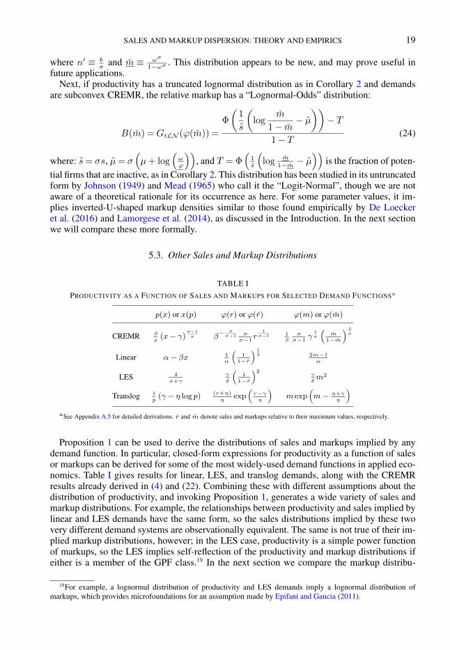
is the fraction of poten-tial firms that are inactive, as in Corollary 2. This distribution has been studied in its untruncatedform by Johnson (1949) and Mead (1965) who call it the “Logit-Normal”, though we are notaware of a theoretical rationale for its occurrence as here. For some parameter values, it im-plies inverted-U-shaped markup densities similar to those found empirically by De Loeckeret al. (2016) and Lamorgese et al. (2014), as discussed in the Introduction. In the next sectionwe will compare these more formally.
5.3. Other Sales and Markup Distributions
TABLE I
PRODUCTIVITY AS A FUNCTION OF SALES AND MARKUPS FOR SELECTED DEMAND FUNCTIONSa
p(x) or x(p) ϕ(r) or ϕ(r) ϕ(m) or ϕ(m)
CREMR β
x(x− γ)
σ−1σ β
− σσ−1 σ
σ−1r
1σ−1 1
βσσ−1
γ1σ
(m
1−m
) 1σ
Linear α− βx 1α
(1
1−r
) 12 2m−1
α
LES δx+γ
γ
δ
(1
1−r
)2γ
δm2
Translog 1p
(γ − η log p) (r+η)
ηexp
(r−γη
)m exp
(m− η+γ
η
)aSee Appendix A.5 for detailed derivations. r and m denote sales and markups relative to their maximum values, respectively.
Proposition 1 can be used to derive the distributions of sales and markups implied by anydemand function. In particular, closed-form expressions for productivity as a function of salesor markups can be derived for some of the most widely-used demand functions in applied eco-nomics. Table I gives results for linear, LES, and translog demands, along with the CREMRresults already derived in (4) and (22). Combining these with different assumptions about thedistribution of productivity, and invoking Proposition 1, generates a wide variety of sales andmarkup distributions. For example, the relationships between productivity and sales implied bylinear and LES demands have the same form, so the sales distributions implied by these twovery different demand systems are observationally equivalent. The same is not true of their im-plied markup distributions, however; in the LES case, productivity is a simple power functionof markups, so the LES implies self-reflection of the productivity and markup distributions ifeither is a member of the GPF class.19 In the next section we compare the markup distribu-
19For example, a lognormal distribution of productivity and LES demands imply a lognormal distribution ofmarkups, which provides microfoundations for an assumption made by Epifani and Gancia (2011).

20
tions implied by these different demand functions with each other and with a given empiricaldistribution.
6. FITTING MARKUPS AND QUANTIFYING MISALLOCATION
So far we have shown how to characterize the exact distributions of various firm outcomes (inparticular firm sales, markups, output in the market equilibrium and socially-optimal output)implied by particular assumptions about the primitives of the model: the structure of demandand the distribution of firm productivities. In this section, we illustrate how, when applied toan actual data set, these theoretical results can be exploited empirically to estimate markupdistributions and to quantify misallocation. In Section 6.1 we introduce the firm-level data onIndian markups used in our econometric analysis. In Section 6.2, we fit the markup distributionsimplied by the theoretical models derived in Section 5 to the markup distributions in the data,and select the best-fitting models. For these models, we show in Section 6.3 how the approachto quantifying misallocation introduced in Section 4 can be implemented. In particular, weuse the estimated parameter values obtained in Section 6.2 to infer the distributions of outputgiven by the market and the one that would be chosen by the planner, and to compare themquantitatively.
As discussed in the introduction, Pareto and lognormal distributions yield very good fits forsales distributions. Thus, since CREMR demands exhibit self-reflection by construction, wewould expect that, when combined with an underlying Pareto or lognormal distribution of pro-ductivities, they will yield a good fit to the distribution of sales.20 By contrast, we are not awareof any previous attempts to fit the distribution of markups and explore its implications for mis-allocation in a theory-consistent way. Hence we focus in this section on fitting the distributionof markups.
6.1. The Data
The data set comes from De Loecker et al. (2016): see Appendix A.6 for more details. Itconsists of 2,457 firm-product observations on markups in Indian manufacturing for the year2001. These markup data are estimated using the so-called “production approach”: markups arecalculated by computing the gap between the output elasticity with respect to variable inputsand the share of those inputs in total revenue.21 This approach assumes cost minimization, atranslog form for the production technology, and that some factor inputs are variable while oth-ers are fixed. However, it does not impose any restrictions on consumer demand nor on marketstructure. Hence it is particularly well-suited to our purpose, which is to compare the perfor-mance of different assumptions about the productivity distribution and the demand function.The approach of De Loecker et al. (2016) has been criticised by Bond et al. (2020); however,the markup estimates we use are not subject to their main critique because they are based onoutput data rather than revenue data.
6.2. Actual Versus Predicted Markup Distributions
The approach we adopt builds directly on the theoretical framework developed in previoussections. Let B(m) denote the markup distribution in the data, while B(m;θ) is the theory-
20As we show in Online Appendices B.3 and B.6, this expectation is confirmed with data on Indian sales andFrench exports respectively, in line with previous literature.
21We do not have access to the confidence intervals for the markups and so we cannot take into account the factthat they were estimated, though it would be straightforward to do so.

SALES AND MARKUP DISPERSION: THEORY AND EMPIRICS 21
consistent predicted distribution. B(m;θ) in turn is implied by an assumed underlying dis-tribution of firm productivities, G(ϕ,θ1), combined with a productivity-markup relationshipimplied by an assumed demand function, ϕ(m;θ2), as given in Table I:
B(m;θ) =G(ϕ(m,θ2),θ1),
where the parameter vector θ is a function of the parameter vectors that characterize the pro-ductivity distribution and the demand function, θ1 and θ2 respectively. For each specificationofG and ϕ, we estimate θ that provides the best fit to the observed distribution B(m). Note thatin all cases θ is of lower dimension than the combined dimensions of θ1 and θ2. Hence, theseparameters are not separately identified, so we cannot fully disentangle the effects of demand-and supply-side influences, though as we shall see we are able to discriminate between differentdemand functions given a maintained hypothesis about the productivity distribution.
To illustrate our approach in the simplest way, we select from the universe of potential speci-fications of productivity distributions and demand functions, a number of the most-widely-usedalternatives which yield closed-form expressions for the implied distributions of firm markupsand output. For the distribution of productivity, we focus on the Pareto and lognormal: bothare plausible in themselves, albeit at different tails of the distribution, and they span a widerange of distributions that have been used in practice. As for our choice of demand functions,we confine attention to the four demand functions presented in Table I in Section 5.3, all ofwhich allow for variable markups.22 It goes without saying that these choices represent onlya limited selection from all possible specifications, but nonetheless a representative sample ofcurrent practice, especially when the constraints of tractability are taken into account.
We have seen how to calculate the theoretical markup distributions in Section 5; furtherdetails are given in Appendix A.7. Using maximum-likelihood (ML) estimation, we fit thetheoretical markup density functions implied by eight different combinations of assumptionsabout the productivity distribution and the demand function. (Details of the estimation processand the code a re available on our websites.) The estimation results are summarized in Table IIand the fitted distributions illustrated in Figure 4.
As the estimates in the third column show, some of the primitive parameters are identified:the Pareto shape parameter k, the lognormal standard deviation of the logs s, and the asymptoticCREMR demand elasticity σ. The other primitive parameters are not identified from our data,and are subsumed into the estimated parameters m and µ: detailed expressions are given in Ta-ble A.II in Appendix A.7. To discriminate between different specifications, we use the Akaikeinformation criterion (AIC), which is well-suited to compare models with different numbers ofparameters, as it trades off goodness of fit and parameter parsimony. The models are ranked inthe table by their AIC values as given in the second-last column. The final column gives therelative likelihood of the other models to the AIC-minimizing one, exp((AICmin−AICi)/2),and can be interpreted as being proportional to the probability that the i’th model minimizesthe estimated information loss. Table II shows that the combination of Pareto productivity andCREMR demands minimizes the AIC. The truncated lognormal with CREMR model comesclosest, but all the others are far inferior by the AIC criterion. The Pareto assumption also givesa better fit with translog demands, but the truncated lognormal does better with LES and lineardemands. These results suggest that the choice of productivity distribution is less importantthan the choice of demand function in fitting the data. Hence in the next subsection, we willexplore misallocation focusing on the two best-fitting CREMR models.
22We do not consider refinements of CES since they cannot match the heterogeneity of markups that we see in thedata.

22
TABLE II
ESTIMATED MARKUP DENSITIES GIVEN ASSUMPTIONS ABOUT PRODUCTIVITY (PARETO (P ) OR TRUNCATEDLOGNORMAL (tLN )) AND DEMAND (CREMR, LINEAR, LES OR TRANSLOG)a
Model Markup PDF Estimated AIC Relativeb(m) Parameters Likelihood
CREMR k(
(σ−1)m
m+σ−mσ
) kσ
(σ−1)m2
((σ−1)m
m+σ−mσ
) σ−kσ
σ = 1.1116049.43
+P k = 1.233
CREMRe−
(log( σm+σ−mσ−1)−µ)2
2(σs)2√
2πms(m+σ−mσ)
1−Φ
log
((σ−1)mm+σ−mσ
)−µ
σs
µ=−49.982
+ s= 6.051 6060.99 0.003
tLN σ = 1.110
Linear √2π
e− (log(2m−1)−µ)2
2s2
s(2m−1)
1−Φ(
log(2m−1)−µs
)µ= 0.054
6180.66 3.2× 10⁻²⁹
+tLN s= 1.228
LES √2π
e− (2 log(m)−µ)2
2s2
ms
1−Φ(
2 log(m)−µs
)µ=−3.234
6184.79 4.1× 10⁻³⁰
+tLN s= 2.732
LES2k(m)2km−2k−1 k = 0.747 6244.63 4.1× 10−43
+P
Translogk(mem)k(m+ 1)m−k−1e−km k = 0.487 6258.08 4.9× 10−46
+P
Translog1√2πs
m+1m
e− (log(mem)−µ)2
2s2
1−Φ(
log(mem)−µs
) µ=−77.6416283.10 1.8× 10−51
+tLN s= 13.064
Linear2k(2m− 1)k (2m− 1)−k−1 k = 1.001 6428.43 5.1× 10−83
+P
aThe ML estimator of the minimum markup m is the minimum empirical markup mmin = 1.001.
6.3. Quantifying Misallocation
Next we want to use the estimated markup-distribution parameters from Section 6.2 for aquantitative comparison of the market and socially optimal distributions of output characterizedin Section 4.2. As we have seen, not all the demand parameters are identified. Nonetheless, wecan use the parameter estimates from the fitted markup distributions to illustrate the divergencebetween market and optimum, and we can exploit the properties of CREMR demands to drawsome general conclusions.
Consider first the case where the productivity distribution is Pareto. As we saw in Sec-tion 4.2, we can combine this with the CREMR productivity-output relationship, using J(x) =G(ϕ(x)), to derive the implied distribution of output in the market equilibrium:
J(x) = 1−(x− γx− γ
)− kσ
= 1− γ kσωk (x− γ)−kσ (25)
The first expression depends on primitive parameters, of which two (k and σ) are observableusing our data, while two (x and γ) are not; whereas in the second only γ is unobservable, since

SALES AND MARKUP DISPERSION: THEORY AND EMPIRICS 23
Histogram of m
m
Den
sity
2 4 6 8 10
0.0
0.2
0.4
0.6
0.8
CREMRLESLinearTranslog
(a) Pareto
Histogram of m
m
Den
sity
2 4 6 8 10
0.0
0.2
0.4
0.6
0.8
CREMRLESLinearTranslog
(b) Truncated Lognormal
FIGURE 4.—Histograms of empirical markup densities compared with fitted densities implied by different as-sumptions about productivity (Pareto or truncated lognormal) and demand (CREMR, LES, Linear or Translog).
ω is a composite parameter that can be calculated from the estimates in Table II. (See (23) andAppendix A.7.) The same holds for the optimal distribution of output with Pareto productivity:
J∗(x) = 1−
((x− γ)
σ−1σ
x
x
(x− γ)σ−1σ
)−k= 1− γ kσ
(ωσ−1
1 + ωσx(x− γ)
1−σσ
)−k(26)
If instead the productivity distribution is a lognormal, left-truncated at ϕ, then the distributionof output in the market equilibrium is:
J(x) =
Φ
( log
(ϕ
(x− γx− γ
) 1σ
)− µ
s
)− T
1− T=
Φ
log
(x− γγ
)− µ
σs
− T1− T
(27)
while the optimal distribution of output is:
J∗(x) =
Φ
( log
(ϕ
((x− γ)
σ−1σ
x
x
(x− γ)σ−1σ
))− µ
s
)− T
1− T
=
Φ
log
(xσ(x− γ)1−σ
γ
)− µx∗
σs
− T1− T
(28)

24
(a) γ = 1.0 (b) γ = 1.5 (c) γ = 2.0
(d) γ = 3.0 (e) γ = 4.0 (f) γ = 5.0
FIGURE 5.—Market versus socially-optimal output profiles: Pareto and CREMR. Each curve shows the market(solid blue line) or socially optimal (dotted red line) density of output, assuming a Pareto distribution of productivitiesand CREMR demands, with estimated parameters k = 1.233, σ = 1.111, and m= 1.001, for different values of γ.
where µx∗ = µ− σ log(σ−1σm)
and T is the fraction of potential firms that are inactive, as in(24). Once again, conditional on γ, the final expressions in (27) and (28) are functions of ob-servables (in this case µ, s, σ, and m). Since γ is the only unobservable parameter in equations(25) to (28), we can illustrate the implied densities of output (in the market equilibrium and inthe social optimum) given the estimates of the other parameters from Table II, conditional ondifferent values of γ. Figures 5 and 6 do this for the Pareto and lognormal cases respectively.
Once again, the choice of the underlying productivity distribution between Pareto and trun-cated lognormal does not seem to be very consequential. Indeed, the similarities between thetwo figures are striking: changes in γ seem to affect the densities in the same way; the optimaland market output densities intersect only once; and the value of output at which they intersectis increasing in γ. We will now prove the last two results more formally.
We have already seen in Proposition 4 that, with CREMR demands, the distribution of out-put in the social optimum first-order stochastically dominates that in the market equilibrium.We can go further and show that, conditional on observables, the critical value of output atwhich the market and optimal output densities intersect (which we denote by xc) is unique andincreases linearly in γ for both Pareto and lognormal distributions:
LEMMA 1: With subconvex CREMR demands, the critical value of output xc at which themarket and planner pdfs intersect is unique and proportional to γ, for any values of the ob-servable parameters (m, k, and σ) when the productivity distribution is Pareto, and for theestimated values of the observable parameters (m, µ, s and σ) when it is lognormal.
The proof is in Appendix A.8. Using the estimated parameters from Table II we find that xcequals 1.465γ in the Pareto case and 1.472γ in the lognormal case. Lemma 1 in turn impliesthat a key measure of misallocation does not depend on γ:

SALES AND MARKUP DISPERSION: THEORY AND EMPIRICS 25
(a) γ = 1.0 (b) γ = 1.5 (c) γ = 2.0
(d) γ = 3.0 (e) γ = 4.0 (f) γ = 5.0
FIGURE 6.—Market versus socially-optimal output profiles: truncated lognormal and CREMR. Each curve showsthe market (solid blue line) or socially optimal (dotted red line) density of output, assuming a truncated lognormal dis-tribution of productivities and CREMR demands, with estimated parameters µ=−49.982, s= 6.051, σ = 1.110,and m= 1.001, for different values of γ.
PROPOSITION 5: With CREMR demands and either Pareto or lognormal productivity, thefraction of firms that lies below the critical value of output xc in both the market equilibriumand the social optimum is independent of γ for given observables: m, k, and σ when theproductivity distribution is Pareto, and m, µ, s and σ when it is lognormal.
The proof is in Appendix A.9. Using the estimated parameter values, we find that J(xc) =0.795 and J∗(xc) = 0.151 in the Pareto case, while J(xc) = 0.797 and J∗(xc) = 0.153 inthe truncated lognormal case. So both the optimal and the market output profiles have moresmaller firms in the truncated lognormal case than in the long-tailed Pareto case, but thesedifferences are small as illustrated by Figures 5 and 6. Furthermore, we can conclude that,independent of γ, in the fitted CREMR-Pareto model, the market gives rise to J(xc)/J
∗(xc) =5.252 times as many “small" firms as a planner would choose, while the corresponding figurein the fitted CREMR-lognormal model is very similar: J(xc)/J
∗(xc) = 5.220. Thus, althoughthe key parameter γ is unobservable, we can draw a strong conclusion about the extent ofmisallocation with CREMR demands: for the parameters that we have estimated, the marketequilibrium has over 5.2 times as many firms that are “too small” relative to the optimum.
7. CONCLUSION
This paper has addressed the question of how to relate the distributions of agent charac-teristics in models of heterogeneous agents. We provide a general necessary and sufficientcondition for consistency between arbitrary assumptions about the distributions of two agentcharacteristics and an arbitrary behavioral model that relates those two characteristics at theindividual level. In the specific context of Melitz-type models of heterogeneous firms compet-ing in monopolistic competition, we showed that our condition implies a new demand function

26
that generalizes the CES. The CREMR or “Constant Revenue Elasticity of Marginal Revenue”demand function is necessary and sufficient for the distributions of firm productivities and firmsales to be members of the same family. It is also necessary and sufficient for Gibrat’s Lawto hold over time under additive separability, it allows for variable markups in a parsimoniousway, it provides a better empirical fit to data on Indian markups drawn from De Loecker et al.(2016) than a number of other better-known demand functions, and it leads to an operationalway of quantifying the deviation of the competitive equilibrium from the social optimum. Allthese results hold for both Pareto and lognormal distributions of productivity, suggesting thatthe choice between these two distributions is less important than the choice between CREMRand other demands.
While we have concentrated on explaining the distributions of firm markups given assump-tions about the distribution of firm productivity, it is clear that our approach has many otherpotential applications. As noted in the introduction, linking observed heterogeneity of out-comes to underlying heterogeneity of agents’ characteristics via an assumed model of agentbehavior is a common research strategy in many fields of economics. Both our general formu-lations and the specific functional forms we have introduced should prove useful in many othercontexts where our results make it possible to move seamlessly between observed distributionsof firm outcomes, hypothesized underlying distributions of firm characteristics, and the behav-ioral model that links them.23 To give just one example, the interaction of distributional anddemand assumptions matters for quantifying the misallocation of resources, as we have shownin Sections 4 and 6. The pioneering study of Hsieh and Klenow (2009) estimated that close tohalf the difference in efficiency between China and India on the one hand and the U.S. on theother could be attributed to an inefficient allocation of labor and capital. However, this was un-der the maintained hypothesis that the output of each industry was a CES aggregate. As Dixitand Stiglitz (1977) and Feenstra and Kee (2008) showed, CES preferences for differentiatedproducts imply that goods markets are constrained efficient. In a non-CES world, inefficiencymay be partly a reflection of goods-market rather than factor-market distortions, with very dif-ferent implications for welfare-enhancing policies.24 In this and other cases, the assumptionsmade about the productivity distribution and demand structure matter for the distribution ofmarkups and other firm outcomes, yet the existing literature gives little guidance on the impli-cations of relaxing the standard assumptions, nor how best to proceed when the assumptions ofthe canonical model do not hold. Our paper has charted a way forward in these directions.
APPENDIX A
This appendix gives technical details, proofs, and extensions. Sections A.1 and A.3 givemore details on the class of Generalized Power Function distributions and the properties ofCREMR demand functions respectively. Sections A.2, A.8, and A.9 give proofs of Proposi-tion 1, Lemma 1 and Proposition 5 respectively. Section A.4 notes some further implications ofProposition 1, Section A.5 sketches the derivations underlying Table I, Section A.6 discusses
23Other examples where our approach may prove fruitful are the interpretation of the trade elasticity, the elasticityof trade with respect to trade costs, which is a constant for many demand functions and Pareto productivities (seeArkolakis et al. (2012), Melitz and Redding (2015), and Arkolakis et al. (2018)) but not when the distribution of firmproductivities is lognormal (see Head et al. (2014) and Bas et al. (2017)); and the granular origins of aggregate fluctu-ations, where Gabaix (2011) and di Giovanni and Levchenko (2012) have shown that considering a discrete numberof draws from a continuous distribution implies that the largest firms can have an impact on aggregate fluctuations,when the distribution of firm size is a power law in the upper tail.
24Arguments along these lines can be found, for example, in Epifani and Gancia (2011), Dhingra and Morrow(2019), and Haltiwanger et al. (2018).
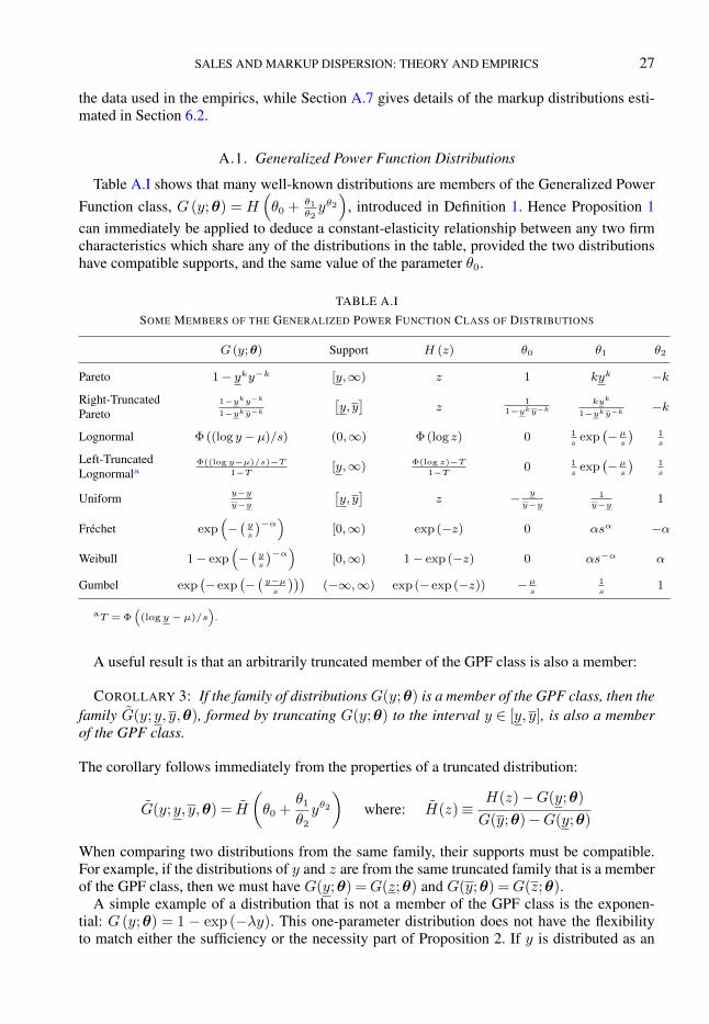
SALES AND MARKUP DISPERSION: THEORY AND EMPIRICS 27
the data used in the empirics, while Section A.7 gives details of the markup distributions esti-mated in Section 6.2.
A.1. Generalized Power Function Distributions
Table A.I shows that many well-known distributions are members of the Generalized PowerFunction class, G (y;θ) = H
(θ0 + θ1
θ2yθ2)
, introduced in Definition 1. Hence Proposition 1can immediately be applied to deduce a constant-elasticity relationship between any two firmcharacteristics which share any of the distributions in the table, provided the two distributionshave compatible supports, and the same value of the parameter θ0.
TABLE A.I
SOME MEMBERS OF THE GENERALIZED POWER FUNCTION CLASS OF DISTRIBUTIONS
G (y;θ) Support H (z) θ0 θ1 θ2
Pareto 1− yky−k [y,∞) z 1 kyk −k
Right-Truncated 1−yky−k
1−yky−k[y, y]
z1
1−yky−kkyk
1−yky−k −kPareto
Lognormal Φ ((log y− µ)/s) (0,∞) Φ (log z) 0 1s
exp(−µs
)1s
Left-Truncated Φ((log y−µ)/s)−T1−T [y,∞) Φ(log z)−T
1−T 0 1s
exp(−µs
)1sLognormala
Uniform y−yy−y
[y, y]
z − y
y−y1
y−y 1
Fréchet exp(−(y
s
)−α)[0,∞) exp (−z) 0 αsα −α
Weibull 1− exp(−(y
s
)−α)[0,∞) 1− exp (−z) 0 αs−α α
Gumbel exp(− exp
(−(y−µs
)))(−∞,∞) exp (− exp (−z)) −µ
s1s
1
aT = Φ((log y− µ)/s
).
A useful result is that an arbitrarily truncated member of the GPF class is also a member:
COROLLARY 3: If the family of distributions G(y;θ) is a member of the GPF class, then thefamily G(y;y, y,θ), formed by truncating G(y;θ) to the interval y ∈ [y, y], is also a memberof the GPF class.
The corollary follows immediately from the properties of a truncated distribution:
G(y;y, y,θ) = H
(θ0 +
θ1
θ2
yθ2)
where: H(z)≡H(z)−G(y;θ)
G(y;θ)−G(y;θ)
When comparing two distributions from the same family, their supports must be compatible.For example, if the distributions of y and z are from the same truncated family that is a memberof the GPF class, then we must have G(y;θ) =G(z;θ) and G(y;θ) =G(z;θ).
A simple example of a distribution that is not a member of the GPF class is the exponen-tial: G (y;θ) = 1 − exp (−λy). This one-parameter distribution does not have the flexibilityto match either the sufficiency or the necessity part of Proposition 2. If y is distributed as an

28
exponential and y = y0zE , then z is distributed as a Weibull: F (z;θ′) = 1 − exp(−λy0z
E).Whereas if both y and z are distributed as exponentials, then y = y0z, i.e., E = 1.
A.2. Proof of Proposition 1
We first give a preliminary lemma, that characterizes the links between the distributions of yand z and the theoretical function linking them:25
LEMMA 2: Given Assumption 1, any two of the following imply the third:(A) y is distributed with CDF G (y), where g(y)≡G′(y)> 0;(B) z is distributed with CDF F (z), where f(z)≡ F ′(z)> 0;(C) Agent behavior is such that: y = v(z), v′(z)> 0;where the functions are related as follows:
(i) (A) and (C) imply (B) with F (z) =G(v(z)) and f(z) = g(v(z))v′(z); similarly, (B) and(C) imply (A) with G(y) = F (v−1(y)) and g(y) = f(v−1(y))d(v
−1(y))
dy.
(ii) (A) and (B) imply (C) with v(z) =G−1(F (z)).
Part (i) of the lemma is a standard result on transformations of variables. Part (ii) is less standard(it is closely related to Lemma 1 of Matzkin (2003)), and requires Assumption 1: characteristicsy(i) and z(i) must refer to the same agent and must be monotonically increasing in i.
The importance of the result is that it allows us to characterize fully the conditions underwhich assumptions about the distributions of two variables and about the relationship that linksthem are mutually consistent. Part (ii) in particular provides an easy way of determining whichspecifications of agent behavior are consistent with particular assumptions about the distribu-tions of agent characteristics. All that is required is to derive the form of v(z) implied by anypair of distributional assumptions.
As already noted, part (i) of Lemma 2 is standard. To prove part (ii), that (A) and (B) imply(C), consider an arbitrary firm i with characteristics y(i) and z(i). Because y(i) and z(i) aremonotonically increasing in i, the fraction of firms with characteristics equal to or less thany(i) and z(i), are equal:
G[y(i)] = F [z(i)] ∀i ∈Ω
Inverting gives y(i) = G−1[F (z(i))]. Since this holds for any firm i ∈ Ω, it follows that y =v(z) =G−1[F (z)], as required. This completes the proof of Lemma 2.
Next, we turn to the proof of Proposition 1 itself. The proof of part (i) is immediate. To showthat (A) and (C) imply (B), assume G (y;θ) = H
(θ0 + θ1
θ2yθ2)
, Gy > 0, and y = y0h(z)E .Then the implied distribution of z is:
F (z;θ) =H
(θ0 +
θ1
θ2
(y0h(z)E
)θ2)=H
(θ0 +
θ′1θ′2h(z)θ
′2
)where: θ′2 = Eθ2 and θ′1
θ′2= θ1
θ2yθ20 so θ′1 = θ1
θ2θ′2y
θ20 = Eθ1y
θ20 . Thus (A) and (C) imply (B). A
similar proof shows that (B) and (C) imply (A).
25We consider a continuum of agents whose characteristics are realizations of a random variable. Because we workwith a continuum, the c.d.f. of this random variable is the actual distribution of these realizations. Henceforward, weuse lower-case variables to describe both a random variable and its realization.

SALES AND MARKUP DISPERSION: THEORY AND EMPIRICS 29
Next, we wish to prove part (ii), that (A) and (B) imply (C). The proof uses a key propertyof the GPF class: the composition of one member of a GPF family and the inverse of an-other is a power function: G−1 (G(z,θ′),θ) = y0z
E . Let ψ equal the distribution in (A): ψ ≡G (y;θ) = H
(θ0 + θ1
θ2yθ2)
, Gy > 0. Inverting the G and H functions gives: y ≡ G−1 (ψ;θ)
and θ0 + θ1θ2yθ2 = H−1(ψ). Eliminating y yields: G−1 (ψ;θ) =
(θ2θ1
(H−1(ψ)− θ0)) 1θ2 . In-
voking part (ii) of Lemma 2, we can state that y = G−1 (F (z;θ′) ;θ), where F (z;θ′) =
H(θ0 +
θ′1θ′2h(z)θ
′2
), Fz > 0, from (B). Hence, substituting for G−1 (ψ;θ) and F (z;θ′) gives:
y =
(θ2
θ1
(H−1
(H
(θ0 +
θ′1θ′2h(z)θ
′2
))− θ0
)) 1θ2
=
(θ2
θ1
((θ0 +
θ′1θ′2h(z)θ
′2
)− θ0
)) 1θ2
= y0h(z)E
where: E =θ′2θ2
and y0 =(θ2θ1
θ′1θ′2
) 1θ2 =
(1E
θ′1θ1
) 1θ2 . Thus (A) and (B) imply (C), which com-
pletes the proof of Proposition 1.
A.3. Properties of CREMR Demand Functions
First, we wish to show that the CREMR property ϕ= (r′)−1 = ϕ0rE is necessary and suffi-
cient for the CREMR demands given in (6). To prove sufficiency, note that, from (6), total andmarginal revenue given CREMR demands are:
r(x) ≡ xp(x) = β (x− γ)σ−1σ r′(x) = p(x) + xp′(x) = β
σ− 1
σ(x− γ)−
1σ (29)
Combining these, the revenue elasticity of marginal revenue is constant, equal to 1σ−1
:
r′(x) = βσσ−1
σ−1
σ r(x)−1
σ−1
To prove necessity, invert equation (5) to obtain r′(x) = ϕ−10 r(x)−E . This is a standard first-
order differential equation in r(x) with constant coefficients. Its solution is:
r(x) =((E + 1)
(ϕ−1
0 x− κ)) 1
E+1 (30)
where κ is a constant of integration. Collecting terms, recalling that r(x) = xp(x), gives the
CREMR demand system (6), where the coefficients are: σ = E+1E
, β = (E+1)1
E+1ϕ− 1E+1
0 , andγ = ϕ0κ. Note that it is the constant κ which makes CREMR more general than CES. Since theCREMR property ϕ = (r′)−1 = ϕ0r
E is both necessary and sufficient for the demands givenin (6), we call the latter CREMR demands.
Next, we wish to derive the demand manifold for CREMR demand functions. This can bedone directly by calculating the elasticity and convexity of demand:
ε=x− γx− γσ
σ and ρ= 2−(
1
x− γσ− 1
(x− γ)σ
)x (31)

30
Eliminating x yields the CREMR demand manifold in the text, equation (11). An alternativeroute to deriving this result that proves useful in Section 3.3 follows Mrázová and Neary (2017),who show that, for a firm with constant marginal cost facing an arbitrary demand function, theelasticities of total and marginal revenue with respect to output can be expressed in terms of theelasticity and convexity of demand. These results yield an expression for the revenue elasticityof marginal revenue which holds for any demand function:
r = ε−1εx
r′ =− 2−ρε−1
x
⇒ r′ =−ε(2− ρ)
(ε− 1)2 r (32)
Equating the coefficient of r to the CREMR elasticity from (30) above, again leads to equation(11). Note that requiring marginal revenue to be positive (ε > 1) and decreasing (ρ < 2) impliesthat σ > 1, just as in the familiar CES case.
The expression for the elasticity of demand in (31) shows that it decreases in output, and sodemand is subconvex, if and only if γ is positive. Further details on this and other properties ofCREMR demands are given in Online Appendix B.2.
A.4. Other Implications of Proposition 1
CEMR
r
CES
CREMR
x
FIGURE A.1.—Demand functions that yield self-reflection between the distributions of firm characteristics.
Section 3 showed that CREMR demands are necessary and sufficient for the distributionsof productivity ϕ and sales revenue r to be members of the same family of the GPF class ofdistributions. In Online Appendix B.1 we use the same approach to characterize the demandfunctions that are necessary and sufficient for self-reflection between the distributions of pro-ductivity and firm output x, and between output and sales revenue. Figure A.1 summarizesschematically all these results: necessary and sufficient for self-reflection of the distributionsof productivity and output is a demand function that we call “CEMR” (Constant Elasticity ofoutput with respect to Marginal Revenue); while CES demands are necessary and sufficientfor self-reflection of the distributions of output and sales. Corollaries of these results are thatCES is sufficient for each of the three bilateral links between distributions, and is necessary andsufficient for all three distributions to have the same form.
A.5. Derivations Underlying Table I
As in Mrázová and Neary (2017), we give the demand functions from a “firm’s-eye view”;many of the parameters taken as given by the firm are endogenous in industry equilibrium. For
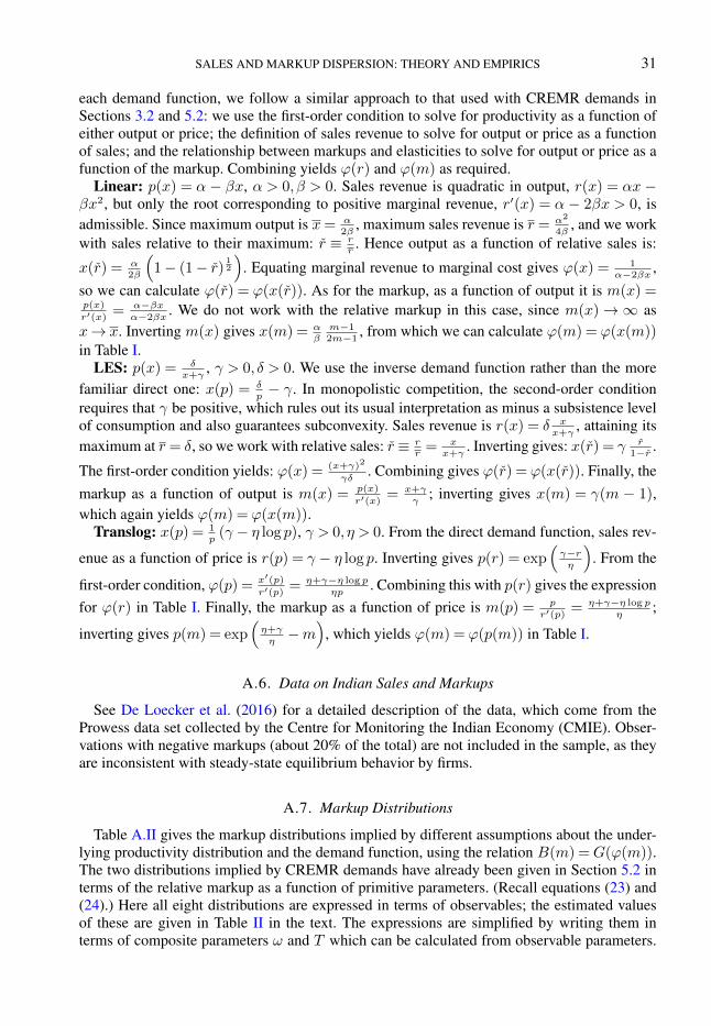
SALES AND MARKUP DISPERSION: THEORY AND EMPIRICS 31
each demand function, we follow a similar approach to that used with CREMR demands inSections 3.2 and 5.2: we use the first-order condition to solve for productivity as a function ofeither output or price; the definition of sales revenue to solve for output or price as a functionof sales; and the relationship between markups and elasticities to solve for output or price as afunction of the markup. Combining yields ϕ(r) and ϕ(m) as required.
Linear: p(x) = α − βx, α > 0, β > 0. Sales revenue is quadratic in output, r(x) = αx −βx2, but only the root corresponding to positive marginal revenue, r′(x) = α − 2βx > 0, isadmissible. Since maximum output is x= α
2β, maximum sales revenue is r = α2
4β, and we work
with sales relative to their maximum: r ≡ rr
. Hence output as a function of relative sales is:
x(r) = α2β
(1− (1− r) 1
2
). Equating marginal revenue to marginal cost gives ϕ(x) = 1
α−2βx,
so we can calculate ϕ(r) = ϕ(x(r)). As for the markup, as a function of output it is m(x) =p(x)
r′(x)= α−βx
α−2βx. We do not work with the relative markup in this case, since m(x)→∞ as
x→ x. Inverting m(x) gives x(m) = αβ
m−12m−1
, from which we can calculate ϕ(m) = ϕ(x(m))in Table I.
LES: p(x) = δx+γ
, γ > 0, δ > 0. We use the inverse demand function rather than the morefamiliar direct one: x(p) = δ
p− γ. In monopolistic competition, the second-order condition
requires that γ be positive, which rules out its usual interpretation as minus a subsistence levelof consumption and also guarantees subconvexity. Sales revenue is r(x) = δ x
x+γ, attaining its
maximum at r = δ, so we work with relative sales: r ≡ rr
= xx+γ
. Inverting gives: x(r) = γ r1−r .
The first-order condition yields: ϕ(x) = (x+γ)2
γδ. Combining gives ϕ(r) = ϕ(x(r)). Finally, the
markup as a function of output is m(x) = p(x)
r′(x)= x+γ
γ; inverting gives x(m) = γ(m − 1),
which again yields ϕ(m) = ϕ(x(m)).Translog: x(p) = 1
p(γ − η log p), γ > 0, η > 0. From the direct demand function, sales rev-
enue as a function of price is r(p) = γ − η log p. Inverting gives p(r) = exp(γ−rη
). From the
first-order condition, ϕ(p) = x′(p)r′(p) = η+γ−η log p
ηp. Combining this with p(r) gives the expression
for ϕ(r) in Table I. Finally, the markup as a function of price is m(p) = p
r′(p) = η+γ−η log p
η;
inverting gives p(m) = exp(η+γ
η−m
), which yields ϕ(m) = ϕ(p(m)) in Table I.
A.6. Data on Indian Sales and Markups
See De Loecker et al. (2016) for a detailed description of the data, which come from theProwess data set collected by the Centre for Monitoring the Indian Economy (CMIE). Obser-vations with negative markups (about 20% of the total) are not included in the sample, as theyare inconsistent with steady-state equilibrium behavior by firms.
A.7. Markup Distributions
Table A.II gives the markup distributions implied by different assumptions about the under-lying productivity distribution and the demand function, using the relation B(m) =G(ϕ(m)).The two distributions implied by CREMR demands have already been given in Section 5.2 interms of the relative markup as a function of primitive parameters. (Recall equations (23) and(24).) Here all eight distributions are expressed in terms of observables; the estimated valuesof these are given in Table II in the text. The expressions are simplified by writing them interms of composite parameters ω and T which can be calculated from observable parameters.

32
TABLE A.II
MARKUP DISTRIBUTIONS IMPLIED BY ASSUMPTIONS ABOUT PRODUCTIVITY (PARETO (P ) OR TRUNCATEDLOGNORMAL (tLN )) AND DEMAND (CREMR, LINEAR, LES OR TRANSLOG)
Demand Function Pareto Productivity Truncated Lognormal Productivity
GP(ϕ) = 1−ϕkϕ−k GtLN (ϕ) =Φ( logϕ−µ
s )−T1−T
CREMR B(m) = 1− ωk(
(σ−1)m
m+σ−σm
)− kσ
B(m) =
Φ
log
((σ−1)mm+σ−mσ
)−µ
sσ
−T1−T
p(x) = βx(x− γ)
σ−1σ ω =
ϕβ
γ1σ
σ−1σ =
((σ−1)mm+σ−σm
) 1σ
µ= σ
µ− log
σσ−1
γ1σβ
T = Φ
(logϕ−µ
s
)= Φ
log
((σ−1)mm+σ−mσ
)−µ
sσ
Linear B(m) = 1−(
2m−1ω
)−kB(m) =
Φ(
log(2m−1)−µs
)−T
1−Tp(x) = α− βx ω = αϕ= 2m− 1 µ= µ+ logα
T = Φ
(logϕ−µ
s
)= Φ
(log(2m−1)−µ
s
)
LES B(m) = 1−(m2
ω
)−kB(m) =
Φ(
2 log(m)−µs
)−T
1−T
p(x) = δx+γ
ω =δϕγ =m2 µ= µ+ log( δγ )
T = Φ
(logϕ−µ
s
)= Φ
(2 log(m)−µ
s
)
Translog B(m) = 1− ωk (mem)−k B(m) =Φ(
log(mem)−µs
)−T
1−T
x(p) = 1p(γ − η log p) ω = e
1+γη ϕ=mem µ= µ+ 1 +
γη
T = Φ
(logϕ−µ
s
)= Φ
(log(mem)−µ
s
)
The table also shows how all observable parameters can be expressed in terms of unobservableprimitive parameters.
A.8. Proof of Lemma 1
Begin with the case of a Pareto productivity distribution. We first show that the market equi-librium and optimal output pdfs cross only once. Using the distributions (25) and (26), wederive the densities j(x) and j∗(x). At any point where these intersect:
γkσk
σωk (x− γ)−
k+σσ = γ
kσk
σ
x− γσx(x− γ)
(ωσ−1
1 + ωσx(x− γ)
1−σσ
)−k⇔
(ωσ
1 + ωσ
)k=x− γσx
(x− γx
)k(33)
Given x > γσ > γ, the right-hand side of (33) is increasing in x. Two densities must intersectat least once, so this proves that they intersect only once. Next, we hypothesize that, for givenvalues of ω, k and σ, the unique solution is linear in γ, so xc = aγ, where a is a constant.Substituting this into (33), γ cancels, leaving an implicit expression for a as a function of ω, kand σ only. Recalling that ω is a composite parameter which can be expressed in terms of m

SALES AND MARKUP DISPERSION: THEORY AND EMPIRICS 33
and σ as in (23), this confirms that, for given values of observables m, k, and σ, xc = aγ is theunique solution of j(x) = j∗(x), which proves Lemma 1 for the Pareto case.
The proof in the case of a lognormal productivity distribution proceeds in the same way.Using the distributions (27) and (28), we derive the densities. At an intersection point:
exp
−(
log
(x− γγ
)− µ)2
2s2σ2
√
2πsσ(x− γ)
1− T=
(x− γσ) exp
(−
(log
(xσ(x− γ)1−σ
γ
)− µx∗
)2
2s2σ2
)√
2πsσx(x− γ)
1− T
⇔ 1 =x− γσx
(1 + ωσ
ωσx− γx
) log
(( ωσ
1+ωσ )σ xσ(x−γ)2−σ
γ2
)−2µ
2s2σ
(34)
Recalling that ω =(
(σ−1)m
m+σ−σm
) 1σ
, for the estimated values of the observable parameters µ, σ, sand m, and any γ, the right-hand side of (34) is monotonically increasing in x for x > γσ > γ.This proves that the densities intersect only once. Next, we test the solution xc = aγ where ais a constant for the estimated parameters. Substituting into (34) yields an implicit expressionfor a as a function of µ, σ, s and ω. This confirms that, for the estimated values of observableparameters µ, σ, s andm, xc = aγ is the unique solution of j(x) = j∗(x), which proves Lemma1 for the lognormal case.
A.9. Proof of Proposition 5
Consider first the Pareto case. Evaluating (25) and (26) at x= xc = aγ yields:
J(xc) = 1− ωk (a− 1)−kσ and J∗(xc) = 1−
(ωσ−1
1 + ωσa(a− 1)
1−σσ
)−kRecalling that ω is a composite parameter which can be expressed in terms of m and σ as in(23), this confirms that, for given values of observablesm, k, and σ, the proportion of firms thatare smaller or equal to xc is independent of γ in both the market and the planner’s distributions.
Similarly, in the lognormal case, evaluating (27) and (28) at x= xc = aγ yields:
J(xc) =
Φ
(log (a− 1)− µ
σs
)− T
1− Tand J∗(xc) =
Φ
(log((a− 1)1−σ)− µx∗
σs
)− T
1− T
Recall that T = Φ(
1σs
(log(
(σ−1)m
m+σ−mσ
)− µ))
and µx∗ = µ− σ log(σ−1σm). So, once again,
conditional on observables m, µ, s and σ, the proportion of firms that are smaller or equal toxc is independent of γ in both the market and the planner’s distributions.
REFERENCES
ANTRÀS, P. AND D. CHOR (2013): “Organizing the Global Value Chain,” Econometrica, 81, 2127–2204.
34
ANTRÀS, P. AND E. HELPMAN (2004): “Global Sourcing,” Journal of Political Economy, 112, 552–580.ARKOLAKIS, C. (2010a): “Market Penetration Costs and the New Consumers Margin in International Trade,” Journal
of Political Economy, 118, 1151–1199.——— (2010b): “Market Penetration Costs and the New Consumers Margin in International Trade: Appendix,” web
appendix, Yale University.——— (2016): “A Unified Theory of Firm Selection and Growth,” Quarterly Journal of Economics, 131, 89–155.ARKOLAKIS, C., A. COSTINOT, D. DONALDSON, AND A. RODRÍGUEZ-CLARE (2018): “The Elusive Pro-
Competitive Effects of Trade,” Review of Economic Studies, 86, 46–80.ARKOLAKIS, C., A. COSTINOT, AND A. RODRÍGUEZ-CLARE (2012): “New Trade Models, Same Old Gains?”
American Economic Review, 102, 94–130.ATKESON, A. AND A. BURSTEIN (2008): “Pricing-to-Market, Trade Costs, and International Relative Prices,” Amer-
ican Economic Review, 98, 1998–2031.AXTELL, R. L. (2001): “Zipf Distribution of U.S. Firm Sizes,” Science, 293, 1818–1820.BAS, M., T. MAYER, AND M. THOENIG (2017): “From Micro to Macro: Demand, Supply, and Heterogeneity in the
Trade Elasticity,” Journal of International Economics, 108, 1–19.BEE, M. AND S. SCHIAVO (2018): “Powerless: Gains from Trade when Firm Productivity is not Pareto Distributed,”
Review of World Economics, 154, 15–45.BEHRENS, K., G. DURANTON, AND F. ROBERT-NICOUD (2014): “Productive Cities: Sorting, Selection, and Ag-
glomeration,” Journal of Political Economy, 122, 507–553.BEHRENS, K., G. MION, Y. MURATA, AND J. SUEDEKUM (2020): “Quantifying the Gap Between Equilibrium and
Optimum under Monopolistic Competition,” Quarterly Journal of Economics, 135, 2299–2360.BERNARD, A. B., S. J. REDDING, AND P. K. SCHOTT (2011): “Multi-Product Firms and Trade Liberalization,”
Quarterly Journal of Economics, 126, 1271–1318.BERTOLETTI, P. AND P. EPIFANI (2014): “Monopolistic Competition: CES Redux?” Journal of International Eco-
nomics, 93, 227–238.BOND, S., A. HASHEMI, G. KAPLAN, AND P. ZOCH (2020): “Some Unpleasant Markup Arithmetic: Production
Function Elasticities and their Estimation from Production Data,” NBER Working Paper No. 27002, http://www.nber.org/papers/w27002.
BUSTOS, P. (2011): “Trade Liberalization, Exports and Technology Upgrading: Evidence on the Impact of MERCO-SUR on Argentinian Firms,” American Economic Review, 101, 304–340.
CABRAL, L. M. AND J. MATA (2003): “On the Evolution of the Firm Size Distribution: Facts and Theory,” AmericanEconomic Review, 93, 1075–1090.
CHANEY, T. (2008): “Distorted Gravity: The Intensive and Extensive Margins of International Trade,” AmericanEconomic Review, 98, 1707–1721.
DE LOECKER, J., P. K. GOLDBERG, A. K. KHANDELWAL, AND N. PAVCNIK (2016): “Prices, Markups and TradeReform,” Econometrica, 84, 445–510.
DEATON, A. AND J. MUELLBAUER (1980): “An Almost Ideal Demand System,” American Economic Review, 70,312–326.
DHINGRA, S. AND J. MORROW (2019): “Monopolistic Competition and Optimum Product Diversity under FirmHeterogeneity,” Journal of Political Economy, 127, 196–232.
DI GIOVANNI, J. AND A. A. LEVCHENKO (2012): “Country Size, International Trade, and Aggregate Fluctuationsin Granular Economies,” Journal of Political Economy, 120, 1083–1132.
DIXIT, A. K. AND J. E. STIGLITZ (1977): “Monopolistic Competition and Optimum Product Diversity,” AmericanEconomic Review, 67, 297–308.
EATON, J. AND S. KORTUM (2002): “Technology, Geography, and Trade,” Econometrica, 70, 1741–1779.EDMOND, C., V. MIDRIGAN, AND D. Y. XU (2015): “Competition, Markups, and the Gains from International
Trade,” American Economic Review, 105, 3183–3221.EECKHOUT, J. (2004): “Gibrat’s Law for (All) Cities,” American Economic Review, 94, 1429–1451.EPIFANI, P. AND G. GANCIA (2011): “Trade, Markup Heterogeneity and Misallocations,” Journal of International
Economics, 83, 1–13.FABINGER, M. AND E. G. WEYL (2012): “Pass-Through and Demand Forms,” mimeo, https://pdfs.semanticscholar.
org/70c0/34b87be44fb02f8e78849a0bdc5f80a5b5f4.pdf.FALLY, T. (2018): “Integrability and Generalized Separability,” NBER Working Paper No. 25025, https://www.nber.
org/papers/w25025.FEENSTRA, R. AND H. L. KEE (2008): “Export Variety and Country Productivity: Estimating the Monopolistic
Competition Model with Endogenous Productivity,” Journal of International Economics, 74, 500–518.FEENSTRA, R. C. (2018): “Restoring the Product Variety and Pro-competitive Gains from Trade with Heterogeneous
Firms and Bounded Productivity,” Journal of International Economics, 110, 16–27.
SALES AND MARKUP DISPERSION: THEORY AND EMPIRICS 35
FEENSTRA, R. C. AND D. E. WEINSTEIN (2017): “Globalization, Markups, and U.S. Welfare,” Journal of PoliticalEconomy, 125, 1040–1074.
FERNANDES, A. M., P. J. KLENOW, S. MELESHCHUK, M. D. PIEROLA, AND A. RODRÍGUEZ-CLARE (2018):“The Intensive Margin in Trade: How Big and How Important?” NBER Working Paper No. 25195, https://www.nber.org/papers/w25195.
GABAIX, X. (1999): “Zipf’s Law for Cities: An Explanation,” Quarterly Journal of Economics, 114, 739–767.——— (2009): “Power Laws in Economics and Finance,” Annual Review of Economics, 1, 255–294.——— (2011): “The Granular Origins of Aggregate Fluctuations,” Econometrica, 79, 733–772.GIBRAT, R. (1931): Les inégalités économiques: applications d’une loi nouvelle, la loi de l’effet proportionnel [Eco-
nomic Inequalities: Applications of a New Law, the Law of Proportionate Effect], Librairie du Recueil Sirey.HALLAK, J. C. AND J. SIVADASAN (2013): “Product and Process Productivity: Implications for Quality Choice and
Conditional Exporter Premia,” Journal of International Economics, 91, 53–67.HALTIWANGER, J., R. S. JARMIN, AND J. MIRANDA (2013): “Who Creates Jobs? Small versus Large versus
Young,” Review of Economics and Statistics, 95, 347–361.HALTIWANGER, J., R. KULICK, AND C. SYVERSON (2018): “Misallocation Measures: The Distortion that Ate the
Residual,” NBER Working Paper No. 24199, https://www.nber.org/papers/w24199.HARRIGAN, J. AND A. RESHEF (2015): “Skill Biased Heterogeneous Firms, Trade Liberalization, and the Skill
Premium,” Canadian Journal of Economics, 48, 1024–1066.HAYASHI, F. (2000): Econometrics, Princeton: Princeton University Press.HEAD, K., T. MAYER, AND M. THOENIG (2014): “Welfare and Trade Without Pareto: Online Appendix,” American
Economic Review, Papers and Proceedings, Additional Materials, 104.HELPMAN, E., M. J. MELITZ, AND S. R. YEAPLE (2004): “Export Versus FDI with Heterogeneous Firms,” Amer-
ican Economic Review, 94, 300–316.HOLMES, T. J. AND J. J. STEVENS (2014): “An Alternative Theory of the Plant Size Distribution, with Geography
and Intra- and International Trade,” Journal of Political Economy, 122, 369–421.HOPENHAYN, H. A. (1992): “Entry, Exit, and Firm Dynamics in Long Run Equilibrium,” Econometrica, 60, 1127–
1150.HSIEH, C.-T. AND P. J. KLENOW (2009): “Misallocation and Manufacturing TFP in China and India,” Quarterly
Journal of Economics, 124, 1403–1448.IJIRI, Y. AND H. A. SIMON (1974): “Interpretations of Departures from the Pareto Curve Firm-Size Distributions,”
Journal of Political Economy, 82, 315–331.JOHNSON, N. (1949): “Systems of Frequency Curves Generated by Methods of Translation,” Biometrika, 36, 149–
176.JOVANOVIC, B. (1982): “Selection and the Evolution of Industry,” Econometrica, 50, 649–670.KIMBALL, M. S. (1995): “The Quantitative Analytics of the Basic Neomonetarist Model,” Journal of Money, Credit
and Banking, 27, 1241–1277.KLENOW, P. J. AND J. L. WILLIS (2016): “Real Rigidities and Nominal Price Changes,” Economica, 83, 443–472.KRUSELL, P. AND A. A. SMITH, JR. (1998): “Income and Wealth Heterogeneity in the Macroeconomy,” Journal of
Political Economy, 106, 867–896.LAMORGESE, A., A. LINARELLO, AND F. WARZYNSKI (2014): “Free Trade Agreements and Firm-Product
Markups in Chilean Manufacturing,” mimeo, ftp://ftp.econ.au.dk/afn/wp/14/wp14_16.pdf.LUTTMER, E. G. (2007): “Selection, Growth, and the Size Distribution of Firms,” Quarterly Journal of Economics,
122, 1103–1144.——— (2010): “Models of Growth and Firm Heterogeneity,” Annual Reviews of Economics, 2, 547–576.——— (2011): “On the Mechanics of Firm Growth,” Review of Economic Studies, 78, 1042–1068.MATSUYAMA, K. AND P. USHCHEV (2017): “Beyond CES: Three Alternative Classes of Flexible Homothetic De-
mand Systems,” CEPR Discussion Paper No. 12210, cepr.org/active/publications/discussion_papers/dp.php?dpno=12210.
MATZKIN, R. L. (2003): “Nonparametric Estimation of Nonadditive Random Functions,” Econometrica, 71, 1339–1375.
MEAD, R. (1965): “A Generalised Logit-Normal Distribution,” Biometrics, 21, 721–732.MELITZ, M. J. (2003): “The Impact of Trade on Intra-Industry Reallocations and Aggregate Industry Productivity,”
Econometrica, 71, 1695–1725.MELITZ, M. J. AND G. I. OTTAVIANO (2008): “Market Size, Trade, and Productivity,” Review of Economic Studies,
75, 295–316.MELITZ, M. J. AND S. J. REDDING (2015): “New Trade Models, New Welfare Implications,” American Economic
Review, 105, 1105–46.MIRRLEES, J. A. (1971): “An Exploration in the Theory of Optimum Income Taxation,” Review of Economic Studies,
38, 175–208.

36
MRÁZOVÁ, M. AND J. P. NEARY (2017): “Not So Demanding: Demand Structure and Firm Behavior,” AmericanEconomic Review, 107, 3835–3874.
——— (2019): “Selection Effects with Heterogeneous Firms,” Journal of the European Economic Association, 17,1294–1334.
NOCCO, A., G. I. P. OTTAVIANO, AND M. SALTO (2014): “Monopolistic Competition and Optimum Product Se-lection,” American Economic Review, 104, 304–09.
PARENTI, M., P. USHCHEV, AND J.-F. THISSE (2017): “Toward a Theory of Monopolistic Ccompetition,” Journalof Economic Theory, 167, 86–115.
POLLAK, R. A. (1972): “Generalized Separability,” Econometrica, 40, 431–453.SIMONOVSKA, I. (2015): “Income Differences and Prices of Tradables: Insights from an Online Retailer,” Review of
Economic Studies, 82, 1612–1656.STIGLITZ, J. E. (1969): “Distribution of Income and Wealth Among Individuals,” Econometrica, 37, 382–397.SUTTON, J. (1997): “Gibrat’s Legacy,” Journal of Economic Literature, 35, 40–59.TINTELNOT, F. (2017): “Global Production with Export Platforms,” Quarterly Journal of Economics, 132, 157–209.ZHELOBODKO, E., S. KOKOVIN, M. PARENTI, AND J.-F. THISSE (2012): “Monopolistic Competition: Beyond the
Constant Elasticity of Substitution,” Econometrica, 80, 2765–2784.
SALES AND MARKUP DISPERSION: THEORY AND EMPIRICS 37
APPENDIX B: SUPPLEMENTARY ONLINE APPENDIX
Section B.1 proves some further corollaries of Proposition 1 beyond those given in Section3. Section B.2 expands on Appendix A.3 with further properties of the CREMR demand func-tion and its demand manifold. Section B.3 uses the Kullback-Leibler Divergence to comparethe goodness of fit for both sales and markups of Indian firms of different assumptions aboutthe productivity distribution and demand. Section B.4 explores how the relative performanceof different specifications, especially the choice of Pareto versus lognormal productivity, is af-fected by truncating the sample. Section B.5 shows that the results are robust to an alternativedistance measure, the QQ estimator. Finally, Section B.6 shows that similar results are obtainedwith a different data set of exports by French firms to Germany.
B.1. Other Implications of Proposition 1
The proof of each of these corollaries to Proposition 1 proceeds in the same way. Given twodistributions y ∼G (y) and z ∼ F (z), we first solve for y = G−1 (F (z)), and then solve theresulting differential equation to derive the implied demand function.
B.1.1. Self-Reflection of Productivity and Output
We first explore the conditions under which output follows the same distribution as pro-ductivity. Proposition 1 implies that a necessary and sufficient condition for this form of self-reflection is that productivity is a simple power function of output: ϕ= ϕ0x
E . Replacing ϕ byr′(x)−1 as before yields a new differential equation in r(x), the solution to which is:
p(x) =1
x(α+ βx
σ−1σ ) (35)
This demand function plays the same role with respect to firm output as the CREMR demandfunction does with respect to firm sales (recall (6)). It is necessary and sufficient for a constantelasticity of marginal revenue with respect to output, equal toE = 1
σ. Hence we call it “CEMR”
for “Constant (Output) Elasticity of Marginal Revenue.”26
Unlike CREMR, there are some precedents for the CEMR class. It has the same functionalform, except with prices and quantities reversed, as the direct PIGL (“Price-Independent Gen-eralized Linearity”) class of Muellbauer (1975).27 In particular, the limiting case where σ ap-proaches one is the inverse translog demand function of Christensen et al. (1975). However,except for the CES (the special case when α= 0), CEMR demands bear little resemblance tocommonly-used demand functions.28 When the common distribution of productivity and outputis a Pareto, we can immediately state a further corollary of Proposition 1:
COROLLARY 4: Given Assumption 1, any two of the following imply the third:(A) The distribution of firm productivity is Pareto: GP(ϕ) = 1−ϕkϕ−k;(B) The distribution of firm output is Pareto: FP(x) = 1− xmx−m;
26“CEMR” rhymes with “seemer,” just as “CREMR” rhymes with “dreamer.”27For this reason, Mrázová and Neary (2017) called it the “inverse PIGL” class of demand functions.28As shown by Mrázová and Neary (2017), the CEMR demand manifold implies a linear relationship between
the convexity and elasticity of demand, passing through the Cobb-Douglas point (ε, ρ) = (1,2): ρ= 2− ε−1
σ. The
manifold for the inverse translog special case (σ→ 1) coincides with the SM locus in Figure 2(b). For smaller firmswhen demand is subconvex, CEMR demands are qualitatively similar to CREMR, except that they are somewhatmore elastic: the CEMR manifold can be written as ε= (2− ρ)σ + 1, while for high ε (so ε− 1≈ ε) the CREMRmanifold is approximately ε= (2− ρ)(σ− 1) + 1.
38
(C) The demand function belongs to the CEMR family in (35);where the parameters are related as follows:
m=k
σand x=
(βσ− 1
σϕ
)σA similar result holds if firm productivities have a lognormal distribution, though, as in theCREMR case of Corollary 2, we have to allow for the possibility that the distribution is left-truncated, as the value of output for the smallest firm may be strictly positive.
COROLLARY 5: Given Assumption 1, any two of the following imply the third:(A) The distribution of firm productivity is truncated lognormal with support [ϕ,+∞):GtLN (ϕ) = Φ((logϕ−µ)/s)−T
1−T ;(B) The distribution of firm output is truncated lognormal with support [x,+∞): FtLN (x) =Φ((logx−µ′′)/s′′)−T
1−T ;(C) The demand function belongs to the CEMR family in (35);where the parameters are related as follows:
s′′ = σs
µ′′ = σ
(µ+ log
(βσ− 1
σ
))
x=
(βσ− 1
σϕ
)σT = Φ((logϕ− µ)/s) = Φ ((logx− µ′′)/s′′)
B.1.2. Self-Reflection of Output and Sales
A final self-reflection corollary of Proposition 1 relates to the case where output and salesfollow the same distribution. This requires that the elasticity of one with respect to the other isconstant, which implies that the demand function must be a CES.29 Formally:
COROLLARY 6: Given Assumption 1, any two of the following imply the third:(A) The distribution of firm output x is a member of the generalized power function class;(B) The distribution of firm sales revenue r is a member of the same family of the generalizedpower function class;(C) The demand function is CES: p(x) = βx−
1σ , where β = x
− 1E
0 and σ = EE−1
.
In the Pareto case, the sufficiency part of this result is familiar from the large literature on theMelitz model with CES demands: it is implicit in Chaney (2008) for example. The necessitypart, taken together with earlier results, shows that it is not possible for all three firm attributes,productivity, sales and revenue, to have the same distribution from the generalized power classunder any demand system other than the CES. Corollary 6 follows immediately from previous
29Suppose that x= x0r(x)E . Recalling that r(x) = xp(x), it follows immediately that the demand function musttake the CES form.
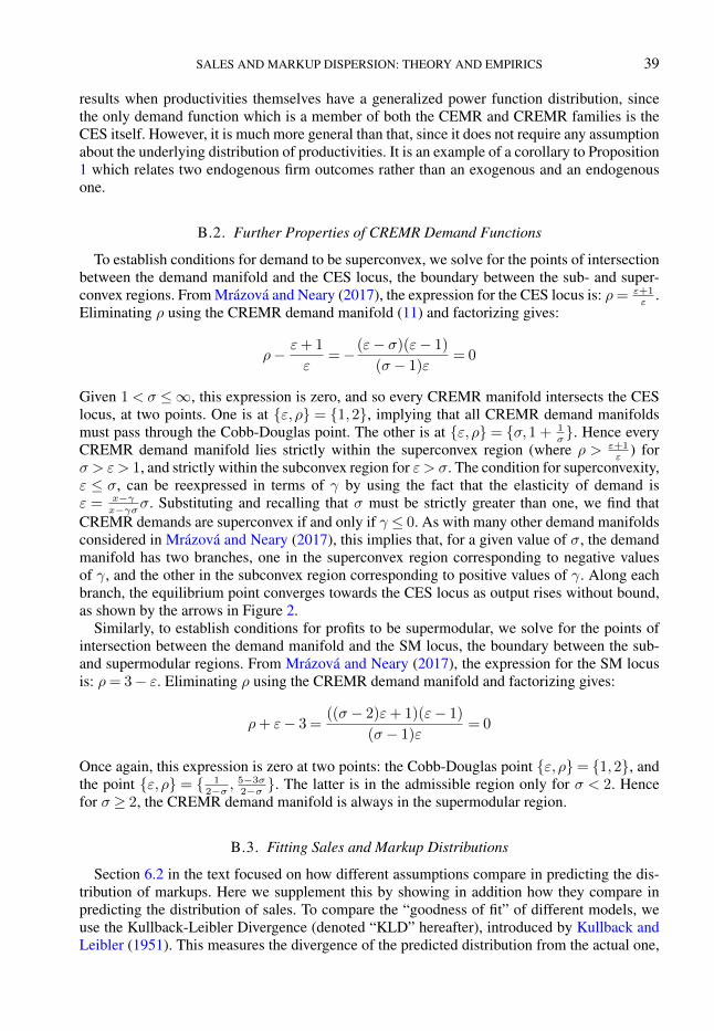
SALES AND MARKUP DISPERSION: THEORY AND EMPIRICS 39
results when productivities themselves have a generalized power function distribution, sincethe only demand function which is a member of both the CEMR and CREMR families is theCES itself. However, it is much more general than that, since it does not require any assumptionabout the underlying distribution of productivities. It is an example of a corollary to Proposition1 which relates two endogenous firm outcomes rather than an exogenous and an endogenousone.
B.2. Further Properties of CREMR Demand Functions
To establish conditions for demand to be superconvex, we solve for the points of intersectionbetween the demand manifold and the CES locus, the boundary between the sub- and super-convex regions. From Mrázová and Neary (2017), the expression for the CES locus is: ρ= ε+1
ε.
Eliminating ρ using the CREMR demand manifold (11) and factorizing gives:
ρ− ε+ 1
ε=−(ε− σ)(ε− 1)
(σ− 1)ε= 0
Given 1< σ ≤∞, this expression is zero, and so every CREMR manifold intersects the CESlocus, at two points. One is at ε, ρ = 1,2, implying that all CREMR demand manifoldsmust pass through the Cobb-Douglas point. The other is at ε, ρ = σ,1 + 1
σ. Hence every
CREMR demand manifold lies strictly within the superconvex region (where ρ > ε+1ε
) forσ > ε > 1, and strictly within the subconvex region for ε > σ. The condition for superconvexity,ε ≤ σ, can be reexpressed in terms of γ by using the fact that the elasticity of demand isε = x−γ
x−γσσ. Substituting and recalling that σ must be strictly greater than one, we find thatCREMR demands are superconvex if and only if γ ≤ 0. As with many other demand manifoldsconsidered in Mrázová and Neary (2017), this implies that, for a given value of σ, the demandmanifold has two branches, one in the superconvex region corresponding to negative valuesof γ, and the other in the subconvex region corresponding to positive values of γ. Along eachbranch, the equilibrium point converges towards the CES locus as output rises without bound,as shown by the arrows in Figure 2.
Similarly, to establish conditions for profits to be supermodular, we solve for the points ofintersection between the demand manifold and the SM locus, the boundary between the sub-and supermodular regions. From Mrázová and Neary (2017), the expression for the SM locusis: ρ= 3− ε. Eliminating ρ using the CREMR demand manifold and factorizing gives:
ρ+ ε− 3 =((σ− 2)ε+ 1)(ε− 1)
(σ− 1)ε= 0
Once again, this expression is zero at two points: the Cobb-Douglas point ε, ρ= 1,2, andthe point ε, ρ = 1
2−σ ,5−3σ2−σ . The latter is in the admissible region only for σ < 2. Hence
for σ ≥ 2, the CREMR demand manifold is always in the supermodular region.
B.3. Fitting Sales and Markup Distributions
Section 6.2 in the text focused on how different assumptions compare in predicting the dis-tribution of markups. Here we supplement this by showing in addition how they compare inpredicting the distribution of sales. To compare the “goodness of fit” of different models, weuse the Kullback-Leibler Divergence (denoted “KLD” hereafter), introduced by Kullback andLeibler (1951). This measures the divergence of the predicted distribution from the actual one,

40
and is asymptotically equivalent to maximum likelihood.30 It equals the information loss fromusing the theory rather than knowing the true distribution. Whereas information scientists typ-ically present KLD values in “bits” (log to base 2) or “nats” (log to base e), units with littleintuitive appeal in economics, we present its values normalized by the value implied by a uni-form distribution. This is an uninformative prior in the spirit of the Laplace principle of in-sufficient reason; it is analogous to the “dartboard” approach to benchmarking the geographicconcentration of manufacturing industry of Ellison and Glaeser (1997), or the “balls and bins”approach to benchmarking the world trade matrix of Armenter and Koren (2014). The value ofthe KLD is unbounded, but a specification that gave a value greater than that implied by a uni-form distribution would be an unsatisfactory explanation of the data. Appendix B.5 shows thatan alternative criterion for choosing between distributions, the QQ estimator, gives qualitativelysimilar results.
TABLE B.I
KLD FOR INDIAN SALES AND MARKUPS COMPARED WITH PREDICTIONS FROM SELECTED PRODUCTIVITYDISTRIBUTIONS AND DEMAND FUNCTIONSa
CREMR Translog LES Linear
A. Sales
Pareto 0.2253 0.1028 0.1837 0.1837
Lognormal 0.0140 0.5825 0.7266 0.7266
B. Markups
Pareto 0.1851 0.2205 0.2191 0.2512
Lognormal 0.1863 0.2228 0.2083 0.2075
aEach KLD value measures the divergence of the predicted from the empirical distribution. A value of zero indicates no divergence, avalue of one a divergence as great as a uniform distribution.
The minimized KLD values for each specification are given in Table B.I and illustrated inFigure B.1. The rankings of different specifications for sales are very different in the Paretoand lognormal cases. Conditional on a Pareto distribution of productivities, CREMR demandsgive the worst fit to sales, with translog demands performing best, and linear-LES intermediatebetween the others. However, the differences between the KLD values for these specificationsare much less than those conditional on lognormal productivities. In this case CREMR doesbest, with translog performing much less well and linear-LES worst of all.
As for the results for markups, these imply exactly the same ranking of different specifica-tions as the estimates given in Table II in Section 6.2, despite the different methodologies used(using individual observations and minimizing the AIC rather than using data grouped in binsand minimizing the KLD as here). Once again, CREMR demands clearly do best, irrespectiveof the assumed distribution, with translog and LES performing at the same level, and lineardoing better under Pareto assumptions but less well in the lognormal case. This reinforces theconclusion drawn in the text that the choice between Pareto and lognormal distributions is lessimportant than the choice between CREMR and other demands.
30The KLD weights the log of the ratio of the estimated density to the empirical density by the empirical densityitself. Many alternative weighting schemes have been proposed, such as Exponential Tilting, which weights the ratioof the empirical density to the estimated density by the estimated density. (See Nevo (2002) for further discussion).

SALES AND MARKUP DISPERSION: THEORY AND EMPIRICS 41
KLD (Sales)
KLD(Markups)
CREMR
TranslogTranslog
LESLES
Linear
Linear
CREMR
0.18
0.20
0.22
0.24
0.26
0.00 0.10 0.20 0.30 0.40 0.50 0.60 0.70 0.80
Lognormal Productivity
Pareto Productivity
FIGURE B.1.—KLD for Indian sales and markups. Data from Table B.I.
TABLE B.II
BOOTSTRAPPED ROBUSTNESS OF THE KLD RANKING: INDIAN SALESa
CREMR + LN CREMR + P TLog + P Lin + P TLog + LN Lin + LN
CREMR + LN – 0% 0% 0% 0% 0%CREMR + P 100% – 0% 0% 0% 0%
TLog + P 100% 100% – 0% 0% 0%Lin + P 100% 100% 100% – 0% 0%
TLog + LN 100% 100% 100% 100% – 0%Lin + LN 100% 100% 100% 100% 100% –
aSee text for explanation. “LN” denotes lognormal, “P” denotes Pareto.
TABLE B.III
BOOTSTRAPPED ROBUSTNESS OF THE KLD RANKING: INDIAN MARKUPSa
CREMR + P CREMR + LN Lin + LN LES + LN LES + P TLog + P TLog + LN Lin + P
CREMR + P – 2% 0% 0% 0% 0% 0% 0%CREMR + LN 98% – 0% 0% 0% 0% 0% 0%
Lin + LN 100% 100% – 0% 0% 0% 0% 0%LES + LN 100% 100% 100% – 0% 0% 0% 0%LES + P 100% 100% 100% 100% – 16% 6% 0%TLog + P 100% 100% 100% 100% 84% – 0% 0%
TLog + LN 100% 100% 100% 100% 94% 100% – 0%Lin + P 100% 100% 100% 100% 100% 100% 100% –
aSee text for explanation.
To assess whether the KLD values in Table B.I are significantly different from one another,we use a bootstrapping approach. We construct one thousand samples of the same size as thedata (i.e., 2,457 observations), by sampling with replacement from the original data. For each
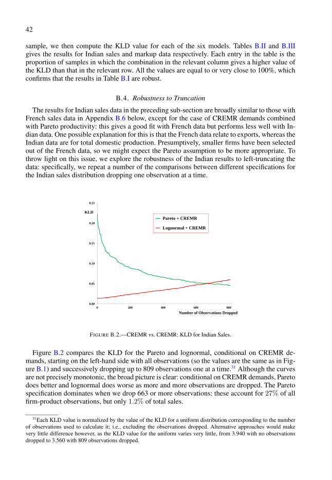
42
sample, we then compute the KLD value for each of the six models. Tables B.II and B.IIIgives the results for Indian sales and markup data respectively. Each entry in the table is theproportion of samples in which the combination in the relevant column gives a higher value ofthe KLD than that in the relevant row. All the values are equal to or very close to 100%, whichconfirms that the results in Table B.I are robust.
B.4. Robustness to Truncation
The results for Indian sales data in the preceding sub-section are broadly similar to those withFrench sales data in Appendix B.6 below, except for the case of CREMR demands combinedwith Pareto productivity: this gives a good fit with French data but performs less well with In-dian data. One possible explanation for this is that the French data relate to exports, whereas theIndian data are for total domestic production. Presumptively, smaller firms have been selectedout of the French data, so we might expect the Pareto assumption to be more appropriate. Tothrow light on this issue, we explore the robustness of the Indian results to left-truncating thedata: specifically, we repeat a number of the comparisons between different specifications forthe Indian sales distribution dropping one observation at a time.
KLD
Number of Observations Dropped
0.00
0.05
0.10
0.15
0.20
0.25
0 200 400 600 800
Pareto + CREMR
Lognormal + CREMR
FIGURE B.2.—CREMR vs. CREMR: KLD for Indian Sales.
Figure B.2 compares the KLD for the Pareto and lognormal, conditional on CREMR de-mands, starting on the left-hand side with all observations (so the values are the same as in Fig-ure B.1) and successively dropping up to 809 observations one at a time.31 Although the curvesare not precisely monotonic, the broad picture is clear: conditional on CREMR demands, Paretodoes better and lognormal does worse as more and more observations are dropped. The Paretospecification dominates when we drop 663 or more observations: these account for 27% of allfirm-product observations, but only 1.2% of total sales.
31Each KLD value is normalized by the value of the KLD for a uniform distribution corresponding to the numberof observations used to calculate it; i.e., excluding the observations dropped. Alternative approaches would makevery little difference however, as the KLD value for the uniform varies very little, from 3.940 with no observationsdropped to 3.560 with 809 observations dropped.
SALES AND MARKUP DISPERSION: THEORY AND EMPIRICS 43
0.00
0.05
0.10
0.15
0.20
0.25
0 20 40 60 80 100 120 140 160 180 200
Pareto + CREMR
Pareto + Linear/LES
Pareto + Translog
KLD
Number of Observations Dropped
FIGURE B.3.—CREMR vs. The Rest, Given Pareto: KLD for Indian Sales.
Figure B.3 shows that a similar pattern emerges when we compare the performance of differ-ent demand functions in explaining the sales distribution, conditional on a Pareto distributionfor productivity. (Note that the horizontal scale differs from that in Figure B.2.) In this case,the CREMR specification overtakes the linear one when we drop 11 or more observations,which account for 0.44% of all firm-product observations, and only 0.0002% of sales. As forthe translog, CREMR overtakes it when we drop 118 or more observations, which account for4.80% of observations, and 0.03% of sales.
These findings confirm that the combination of CREMR demand and Pareto productivitiesfits the sales data relatively better when the smallest observations are dropped. They also makeprecise the pattern observed in many datasets, whereby the Pareto assumption outperforms thelognormal in the right tail of the sales distribution. For example, Figure B.2 shows that therelevant region in the right tail begins at exactly 663 observations.
B.5. Robustness to Divergence Criterion: The QQ Estimator
To check the robustness of our results, we consider an alternative criterion to the KLD forcomparing predicted and actual distributions. Here we consider the QQ estimator, developedby Kratz and Resnick (1996), and previously used by Head et al. (2014) and Nigai (2017). Thisestimator does not have the same desirable theoretical properties as the KLD, in particular itis not asymptotically equivalent to maximum likelihood, but it has a simple interpretation. Itequals the parameter vector θ∗ that minimizes the sum of the squared deviations of the quantilesof the predicted distribution from those of the actual distribution:
QQ(F || F (·;θ)) =n∑i=1
(log qi − log qi(θ))2
where qi = F−1(i/n) is the i’th quantile observed in the data, while qi(θ) = F−1(i/n;θ) isthe i’th quantile predicted by the theory.
To implement the QQ estimator we need analytic expressions for the quantiles of the salesand markup distributions under each of the eight combinations of assumptions about demand

44
TABLE B.IV
QUANTILE FUNCTIONS FOR SALES DISTRIBUTIONS IMPLIED BY ASSUMPTIONS ABOUT PRODUCTIVITY(PARETO (P ) OR TRUNCATED LOGNORMAL (tLN )) AND DEMAND (CREMR, LINEAR, LES OR TRANSLOG)a
Demand Function Pareto Productivity Truncated Lognormal Productivity
GP(ϕ) = 1−ϕkϕ−k GtLN (ϕ) =Φ( logϕ−µ
s )−T1−T
CREMRQ(y) = βσ
(σ−1σϕ)σ−1
(1− y)1−σk Q(y) = βσ
(σ−1σeµ+sΦ−1(y(1−T )+T )
)σ−1
p(x) = βx(x− γ)
σ−1σ
LinearQ(y) =
α2ϕ2−(1−y)2k
4βϕ2 Q(y) = α2−e−2(µ+sΦ−1(y(1−T )+T ))
4βp(x) = α− βx
LESQ(y) = δ−
√γδϕ(1− y) 1
2k Q(y) = δ−√γδ
e12 (µ+sΦ−1(y(1−T )+T ))p(x) = δ
x+γ
TranslogQ(y) = η
(W(ϕe
1+γη (1− y)
− 1k
)− 1
)Q(y) = η
(W(e1+
γη+µ+sΦ−1(y(1−T )+T )
)− 1
)x(p) = γ−η log p
p
aΦ(·): c.d.f. of a standard normal;W(·): the Lambert function.
TABLE B.V
QUANTILE FUNCTIONS FOR MARKUP DISTRIBUTIONS IMPLIED BY ASSUMPTIONS ABOUT PRODUCTIVITY(PARETO (P ) OR TRUNCATED LOGNORMAL (tLN )) AND DEMAND (CREMR, LINEAR, LES OR TRANSLOG)a
Demand Function Pareto Productivity Truncated Lognormal Productivity
GP(ϕ) = 1−ϕkϕ−k GtLN (ϕ) =Φ( logϕ−µ
s )−T1−T
CREMR Q(y) = σσ−1
1(1+ω−σ(1−y)
σk) Q(y) = σ
σ−11
1+e−µ−sσΦ−1(y(1−T )+T )
p(x) = βx(x− γ)
σ−1σ ω =
ϕβ
γ1σ
σ−1σ µ= σ
µ− log
σσ−1
γ1σβ
Linear Q(y) = 12
(1 + ω (1− y)−
1k
)Q(y) = 1
2
(1 + eµ+sΦ−1(y(1−T )+T )
)p(x) = α− βx ω = αϕ µ= µ+ logα
LES Q(y) =
√ω (1− y)−1/k Q(y) = e
12 (µ+sΦ−1(y(1−T )+T ))
p(x) = δx+γ
ω =δϕγ µ= µ+ log( δγ )
Translog Q(y) =W(ω (1− y)−1/k
)Q(y) =W
(eµ+sΦ−1(y(1−T )+T )
)x(p) = γ−η log p
pω = e
1+γη ϕ µ= µ+ 1 +
γη
aΦ(·): c.d.f. of a standard normal;W(·): the Lambert function.

SALES AND MARKUP DISPERSION: THEORY AND EMPIRICS 45
and the distribution of productivity we consider. These are given in Tables B.IV and B.V. Weset the number of quantiles n equal to 100. The resulting values of the QQ estimator for Indiansales and markups are given in Table B.VI, and they are illustrated in Figure B.4.
Comparing Table B.VI and Figure B.4 with Table B.I and Figure B.1 in Appendix B.3 re-spectively, it is evident that the results based on the QQ estimator are qualitatively very similarto those for the KLD. In particular, the Pareto assumption gives a better fit for sales than formarkups, except in the CREMR case; while the lognormal assumption tends to give a betterfit for markups than for sales. Comparing different demand functions, CREMR demands givea better fit to the markup distribution than any other demands, irrespective of which produc-tivity distribution is assumed. As for sales, the results differ between the Pareto and lognormalcases. Conditional on lognormal, CREMR again performs much better, whereas, conditionalon Pareto, it performs least well, with the translog doing best. The only qualitative differencebetween the results using the two criteria is that with the QQ estimator the translog does some-what better than the LES in fitting the markup distribution. Overall, we can conclude that therankings given in Section 6.1 are not unduly sensitive to our choice of criterion for comparingactual and predicted distributions.
TABLE B.VI
QQ ESTIMATOR FOR INDIAN SALES AND MARKUPS
CREMR Translog LES Linear
A. Sales
Pareto 58.939 12.693 24.484 24.484
Lognormal 3.078 116.918 133.274 133.274
B. Markups
Pareto 0.113 0.978 1.133 3.606
Lognormal 0.110 0.990 0.340 0.325
B.6. French Exports to Germany
The Indian data used in Section 6 have the great advantage that they give both sales andmarkups for all firms. This is important, for example, in allowing us to discriminate betweenCES and CREMR, whose implications for sales are observationally equivalent. However, rel-ative to many data sets used in recent trade applications, they refer to total sales rather thanexports and they cover a relatively small number of firms. Hence it is useful to repeat the anal-ysis on a more conventional data set on export sales, even if this does not give information onmarkups. We do this in this section, using data on the universe of French exports to Germanyin 2005, drawn from the same source as that used by Head et al. (2014).32
As with the Indian data in the text, we use the KLD as the criterion to determine how welldifferent assumptions fit the data. Table B.VII gives the values of the KLD measuring the di-vergence from the empirical sales distribution from the distributions implied by CREMR/CES,translog and linear demand functions combined with either Pareto or lognormal productivities.These distributions are calculated by combining the relevant productivity distribution with the
32The data set contains 161,191 firm-product observations on export sales by 27,550 firms: 5.85 products per firm.

46
0.00
0.50
1.00
1.50
2.00
2.50
3.00
3.50
4.00
0.0 20.0 40.0 60.0 80.0 100.0 120.0 140.0
Lognormal Productivity
Pareto Productivity
QQ (Sales)
QQ(Markups)
CREMR
Translog
Translog
LES
LES
Linear
Linear
CREMR
FIGURE B.4.—QQ Estimator for Indian sales and markups.
TABLE B.VII
KLD FOR FRENCH EXPORTS COMPARED WITH PREDICTIONS FROM SELECTED DEMAND FUNCTIONS ANDPRODUCTIVITY DISTRIBUTIONS
CREMR/CES Translog Linear and LES
Pareto 0.0012 0.3819 0.4711Lognormal 0.0001 0.7315 0.8314
relationships between productivity and sales given in Table I. (Recall from that table that thelinear and LES specifications are observationally equivalent.) Each entry in the table is thevalue of the KLD that measures the information loss when the combination of assumptionsindicated by the row and column is used to explain the observed distribution of sales. (As withthe Indian data in Section 6, the data are normalized by the value of the KLD for a uniformdistribution, which for this data set is 6.8082.)
Turning to the results in Table B.VII, the values of the minimized KLD show that, conditionalon CREMR or CES demands, the lognormal provides a better overall fit than the Pareto: 0.0001as opposed to 0.0012. However, the difference between distributions turns out to be much lesssignificant than those between different specifications of demand. The KLD values for thetranslog and linear/LES specifications are much higher than for the CREMR case, as shown inthe third and fourth columns of Table B.VII, with the Pareto now preferred to the lognormal.The overwhelming conclusion from these results is that, if we want to fit the distribution of salesin this data set, then the choice between Pareto and lognormal distributions is less importantthan the choice between CREMR and other demands. This is broadly in line with the results forIndian sales data in Section 6, especially when we exclude the smallest firms as in Section B.4.
Table B.VIII repeats for French exports data the bootstrapping comparisons presented in Ta-bles B.II and B.III for Indian sales and markup data respectively. It is clear that the comparisonsbetween different values of the KLD for the French data shown in Table B.VII are just as robustas those for the Indian data shown in Table B.I and Figure B.1 in the text.

SALES AND MARKUP DISPERSION: THEORY AND EMPIRICS 47
TABLE B.VIII
BOOTSTRAPPED ROBUSTNESS OF THE KLD RANKING: FRENCH SALESa
CREMR + LN CREMR + P TLog + P Lin + P TLog + LN Lin + LN
CREMR + LN – 0% 0% 0% 0% 0%CREMR + P 100% – 0% 0% 0% 0%
TLog + P 100% 100% – 0% 0% 0%Lin + P 100% 100% 100% – 0% 0%
TLog + LN 100% 100% 100% 100% – 0.3%Lin + LN 100% 100% 100% 100% 99.7% –
aSee text for explanation.
REFERENCES
ARMENTER, R. AND M. KOREN (2014): “A Balls-and-Bins Model of Trade,” American Economic Review, 104,2127–2151.
CHANEY, T. (2008): “Distorted Gravity: The Intensive and Extensive Margins of International Trade,” AmericanEconomic Review, 98, 1707–1721.
CHRISTENSEN, L. R., D. W. JORGENSON, AND L. J. LAU (1975): “Transcendental Logarithmic Utility Functions,”American Economic Review, 65, 367–383.
ELLISON, G. AND E. L. GLAESER (1997): “Geographic Concentration in U.S. Manufacturing Industries: A Dart-board Approach,” Journal of Political Economy, 105, 889–927.
HEAD, K., T. MAYER, AND M. THOENIG (2014): “Welfare and Trade Without Pareto,” American Economic Review,Papers and Proceedings, 104, 310–316.
KRATZ, M. AND S. I. RESNICK (1996): “The QQ-estimator and heavy tails,” Stochastic Models, 12, 699–724.KULLBACK, S. AND R. A. LEIBLER (1951): “On Information and Sufficiency,” Annals of Mathematical Statistics,
22, 79–86.MRÁZOVÁ, M. AND J. P. NEARY (2017): “Not So Demanding: Demand Structure and Firm Behavior,” American
Economic Review, 107, 3835–3874.MUELLBAUER, J. (1975): “Aggregation, Income Distribution and Consumer Demand,” Review of Economic Studies,
42, 525–543.NEVO, A. (2002): “Sample Selection and Information-Theoretic Alternatives to GMM,” Journal of Econometrics,
107, 149–157.NIGAI, S. (2017): “A Tale of Two Tails: Productivity Distribution and the Gains from Trade,” Journal of International
Economics, 104, 44–62.


![Walsch.neale Print Storm-before-calm Ch1-3 Wbuylinks[1]](https://static.fdocuments.net/doc/165x107/54e8a7454a79594d398b46d0/walschneale-print-storm-before-calm-ch1-3-wbuylinks1.jpg)