January 2016 - Jerry Dwyerjerrydwyer.com/pdf/Clemson/Topic2DifferenceEquations.pdf · Solutions to...
82
Difference Equations Gerald P. Dwyer Clemson University January 2016
Transcript of January 2016 - Jerry Dwyerjerrydwyer.com/pdf/Clemson/Topic2DifferenceEquations.pdf · Solutions to...
Difference Equations
Gerald P. Dwyer
Clemson University
January 2016
Outline
1 Difference EquationsIntroduction
OperatorsMultipliers and Impulse Response Functions
Solutions to Difference EquationsSolution by IterationGeneral method of solution
Solve First-Order Difference Equation
Method of Undetermined CoefficientsLag Operator to Solve EquationsSecond-order difference equationSummary
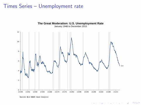
Times Series – Unemployment rate
5.0
0
2
4
6
8
10
12
1/1/48 1/1/53 1/1/58 1/1/63 1/1/68 1/1/73 1/1/78 1/1/83 1/1/88 1/1/93 1/1/98 1/1/03 1/1/08 1/1/13
The Great Moderation: U.S. Unemployment RateJanuary 1948 to December 2015
Sources: BLS, NBER, Haver Analytics
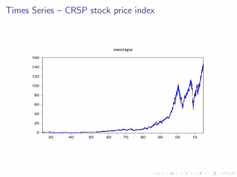
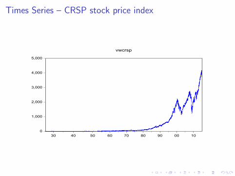
Times Series – CRSP stock price index
0
20
40
60
80
100
120
140
160
30 40 50 60 70 80 90 00 10
vwcrspx
Times Series – CRSP stock price index
0
1,000
2,000
3,000
4,000
5,000
30 40 50 60 70 80 90 00 10
vwcrsp
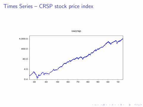
Times Series – CRSP stock price index
4,000.0
400.0
40.0
4.0
0.430 40 50 60 70 80 90 00 10
vwcrsp
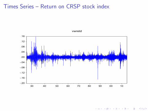
Times Series – Return on CRSP stock index
-.20
-.16
-.12
-.08
-.04
.00
.04
.08
.12
.16
30 40 50 60 70 80 90 00 10
vwretd
Autoregressions
Unemployment rate
CRSP price index
CRSP return
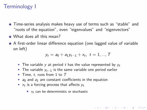
Terminology I
Time-series analysis makes heavy use of terms such as “stable” and“roots of the equation”, even “eigenvalues” and “eigenvectors”
What does all this mean?
A first-order linear difference equation (one lagged value of variableon left)
yt = a0 + a1yt−1 + xt , t = 1, ...,T
I The variable y at period t has the value represented by ytI The variable yt−1 is the same variable one period earlierI Time, t, runs from 1 to TI a0 and a1 are constant coefficients in the equationI xt is a forcing process that affects yt
F xt can be deterministic or stochastic
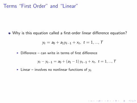
Terms “First Order” and “Linear”
Why is this equation called a first-order linear difference equation?
yt = a0 + a1yt−1 + xt , t = 1, ...,T
I Difference – can write in terms of first difference
yt − yt−1 = a0 + (a1 − 1) yt−1 + xt , t = 1, ...,T
I Linear – involves no nonlinear functions of yt
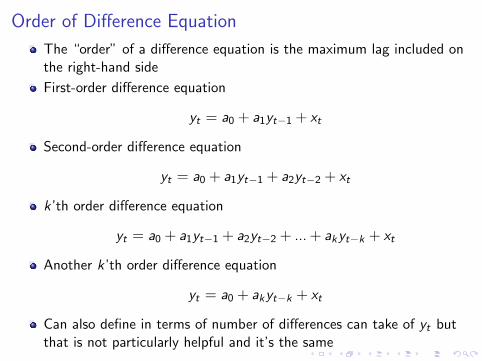
Order of Difference Equation
The “order” of a difference equation is the maximum lag included onthe right-hand side
First-order difference equation
yt = a0 + a1yt−1 + xt
Second-order difference equation
yt = a0 + a1yt−1 + a2yt−2 + xt
k ’th order difference equation
yt = a0 + a1yt−1 + a2yt−2 + ... + akyt−k + xt
Another k ’th order difference equation
yt = a0 + akyt−k + xt
Can also define in terms of number of differences can take of yt butthat is not particularly helpful and it’s the same

Deterministic and stochastic
“Deterministic” means perfectly predictable from its own past
I For example trend xt = bt with b knownI Quarterly dummy variablesI A deterministic difference equation
yt = a0 + a1yt−1 + bt, t = 1, ...,T
“Stochastic” means evolves according to a probability law, e.g.xt = εt ∼ N(0, 1)
I Another word is “random”
F Does not mean “arbitrary”
I “Random” means for example xt = εt ∼ N(0, 1)I A stochastic difference equation
yt = a0 + a1yt−1 + εt , t = 1, ...,T
εt ∼ N(
0, σ2)
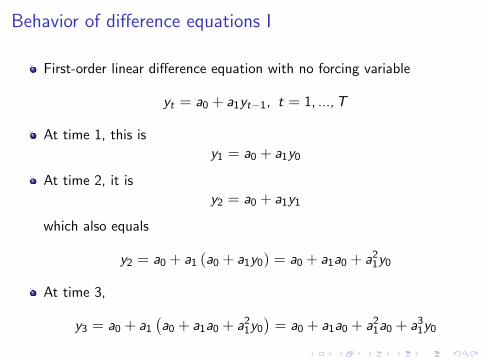
Behavior of difference equations I
First-order linear difference equation with no forcing variable
yt = a0 + a1yt−1, t = 1, ...,T
At time 1, this is
y1 = a0 + a1y0
At time 2, it is
y2 = a0 + a1y1
which also equals
y2 = a0 + a1 (a0 + a1y0) = a0 + a1a0 + a21y0
At time 3,
y3 = a0 + a1(a0 + a1a0 + a21y0
)= a0 + a1a0 + a21a0 + a31y0
Behavior of difference equations II
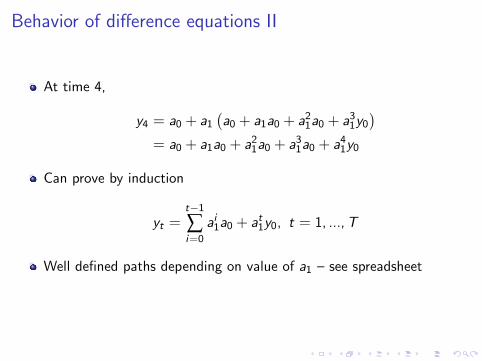
At time 4,
y4 = a0 + a1(a0 + a1a0 + a21a0 + a31y0
)= a0 + a1a0 + a21a0 + a31a0 + a41y0
Can prove by induction
yt =t−1∑i=0
ai1a0 + at1y0, t = 1, ...,T
Well defined paths depending on value of a1 – see spreadsheet
Operators I
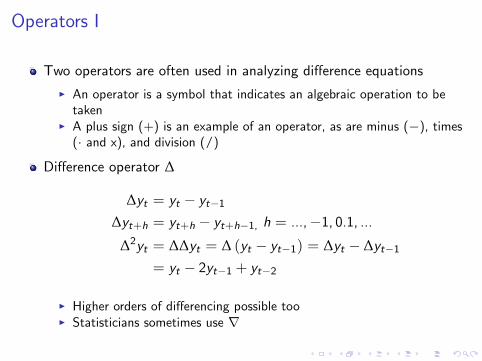
Two operators are often used in analyzing difference equations
I An operator is a symbol that indicates an algebraic operation to betaken
I A plus sign (+) is an example of an operator, as are minus (−), times(· and x), and division (/)
Difference operator ∆
∆yt = yt − yt−1
∆yt+h = yt+h − yt+h−1, h = ...,−1, 0.1, ...
∆2yt = ∆∆yt = ∆ (yt − yt−1) = ∆yt − ∆yt−1
= yt − 2yt−1 + yt−2
I Higher orders of differencing possible tooI Statisticians sometimes use ∇
Operators II
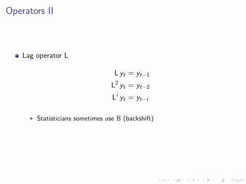
Lag operator L
L yt = yt−1
L2 yt = yt−2
Li yt = yt−i
I Statisticians sometimes use B (backshift)
Polynomial in lag operator
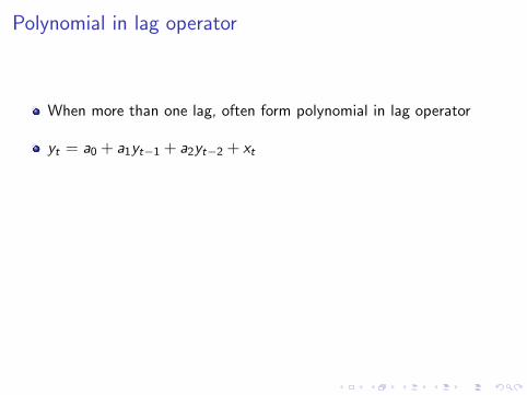
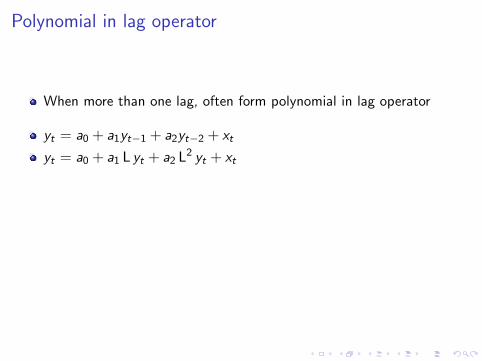
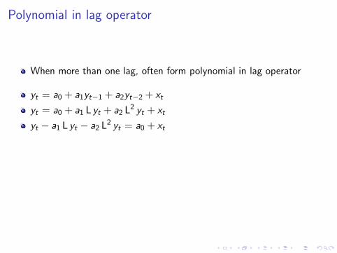
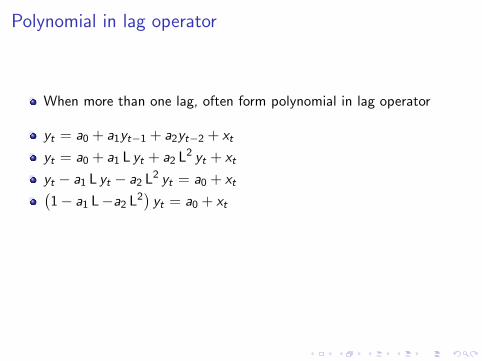
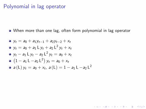
When more than one lag, often form polynomial in lag operator
yt = a0 + a1yt−1 + a2yt−2 + xt
yt = a0 + a1 L yt + a2 L2 yt + xt
yt − a1 L yt − a2 L2 yt = a0 + xt(1− a1 L−a2 L2
)yt = a0 + xt
a (L) yt = a0 + xt , a (L) = 1− a1 L−a2 L2
or yt = a0 + a∗ (L) yt−1 + xt , a∗ (L) =
1
∑i=1
ai Li = a1 + a2 L
Polynomial in lag operator
When more than one lag, often form polynomial in lag operator
yt = a0 + a1yt−1 + a2yt−2 + xt
yt = a0 + a1 L yt + a2 L2 yt + xt
yt − a1 L yt − a2 L2 yt = a0 + xt
(1− a1 L−a2 L2
)yt = a0 + xt
a (L) yt = a0 + xt , a (L) = 1− a1 L−a2 L2
or yt = a0 + a∗ (L) yt−1 + xt , a∗ (L) =
1
∑i=1
ai Li = a1 + a2 L
Polynomial in lag operator
When more than one lag, often form polynomial in lag operator
yt = a0 + a1yt−1 + a2yt−2 + xt
yt = a0 + a1 L yt + a2 L2 yt + xt
yt − a1 L yt − a2 L2 yt = a0 + xt(1− a1 L−a2 L2
)yt = a0 + xt
a (L) yt = a0 + xt , a (L) = 1− a1 L−a2 L2
or yt = a0 + a∗ (L) yt−1 + xt , a∗ (L) =
1
∑i=1
ai Li = a1 + a2 L
Polynomial in lag operator
When more than one lag, often form polynomial in lag operator
yt = a0 + a1yt−1 + a2yt−2 + xt
yt = a0 + a1 L yt + a2 L2 yt + xt
yt − a1 L yt − a2 L2 yt = a0 + xt(1− a1 L−a2 L2
)yt = a0 + xt
a (L) yt = a0 + xt , a (L) = 1− a1 L−a2 L2
or yt = a0 + a∗ (L) yt−1 + xt , a∗ (L) =
1
∑i=1
ai Li = a1 + a2 L
Lag Operator
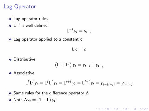
Lag operator rules
L−i is well definedL−i yt = yt+i
Lag operator applied to a constant c
L c = c
Distributive (Li + Lj
)yt = yt−i + yt−j
Associative
Li Lj yt = Lj Li yt = Li+j yt = Lj+i yt = yt−(i+j) = yt−i−j
Same rules for the difference operator ∆Note ∆yt = (1− L) yt
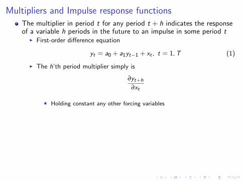
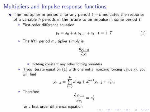
Multipliers and Impulse response functionsThe multiplier in period t for any period t + h indicates the responseof a variable h periods in the future to an impulse in some period t
I First-order difference equation
yt = a0 + a1yt−1 + xt , t = 1,T (1)
I The h’th period multiplier simply is
∂yt+h
∂xt
F Holding constant any other forcing variables
I If you iterate equation (1) with one initial nonzero forcing value xt , youwill find
yt+h =h
∑i=0
ai1a0 + ah+11 yt−1 + ah1xt
I Therefore∂yt+h
∂xt= ah1
for a first-order difference equation
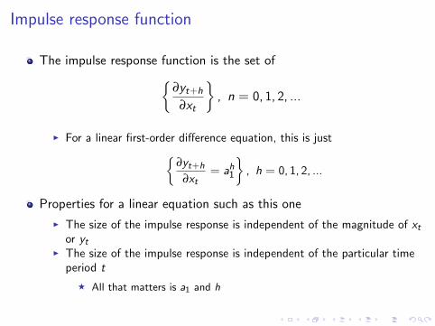
Impulse response function
The impulse response function is the set of{∂yt+h
∂xt
}, n = 0, 1, 2, ...
I For a linear first-order difference equation, this is just{∂yt+h
∂xt= ah1
}, h = 0, 1, 2, ...
Properties for a linear equation such as this one
I The size of the impulse response is independent of the magnitude of xtor yt
I The size of the impulse response is independent of the particular timeperiod t
F All that matters is a1 and h
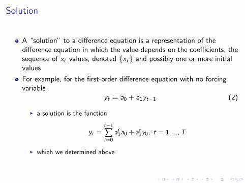
Solution
A “solution” to a difference equation is a representation of thedifference equation in which the value depends on the coefficients, thesequence of xt values, denoted {xt} and possibly one or more initialvalues
For example, for the first-order difference equation with no forcingvariable
yt = a0 + a1yt−1 (2)
I a solution is the function
yt =t−1∑i=0
ai1a0 + at1y0, t = 1, ...,T
I which we determined above
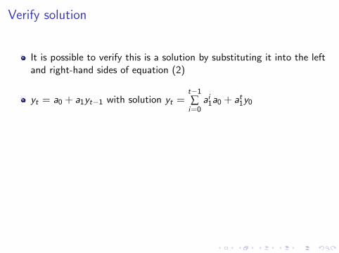
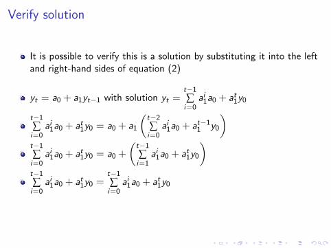
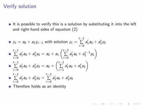
Verify solution
It is possible to verify this is a solution by substituting it into the leftand right-hand sides of equation (2)
yt = a0 + a1yt−1 with solution yt =t−1∑i=0
ai1a0 + at1y0
t−1∑i=0
ai1a0 + at1y0 = a0 + a1
(t−2∑i=0
ai1a0 + at−11 y0
)t−1∑i=0
ai1a0 + at1y0 = a0 +
(t−1∑i=1
ai1a0 + at1y0
)t−1∑i=0
ai1a0 + at1y0 =t−1∑i=0
ai1a0 + at1y0
Therefore holds as an identity
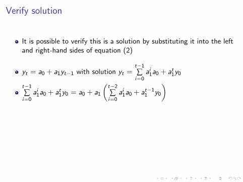
Verify solution
It is possible to verify this is a solution by substituting it into the leftand right-hand sides of equation (2)
yt = a0 + a1yt−1 with solution yt =t−1∑i=0
ai1a0 + at1y0
t−1∑i=0
ai1a0 + at1y0 = a0 + a1
(t−2∑i=0
ai1a0 + at−11 y0
)
t−1∑i=0
ai1a0 + at1y0 = a0 +
(t−1∑i=1
ai1a0 + at1y0
)t−1∑i=0
ai1a0 + at1y0 =t−1∑i=0
ai1a0 + at1y0
Therefore holds as an identity
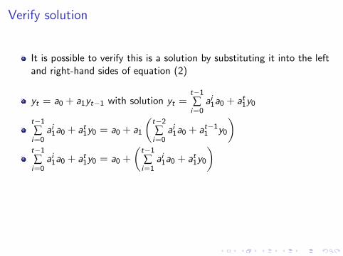
Verify solution
It is possible to verify this is a solution by substituting it into the leftand right-hand sides of equation (2)
yt = a0 + a1yt−1 with solution yt =t−1∑i=0
ai1a0 + at1y0
t−1∑i=0
ai1a0 + at1y0 = a0 + a1
(t−2∑i=0
ai1a0 + at−11 y0
)t−1∑i=0
ai1a0 + at1y0 = a0 +
(t−1∑i=1
ai1a0 + at1y0
)
t−1∑i=0
ai1a0 + at1y0 =t−1∑i=0
ai1a0 + at1y0
Therefore holds as an identity
Verify solution
It is possible to verify this is a solution by substituting it into the leftand right-hand sides of equation (2)
yt = a0 + a1yt−1 with solution yt =t−1∑i=0
ai1a0 + at1y0
t−1∑i=0
ai1a0 + at1y0 = a0 + a1
(t−2∑i=0
ai1a0 + at−11 y0
)t−1∑i=0
ai1a0 + at1y0 = a0 +
(t−1∑i=1
ai1a0 + at1y0
)t−1∑i=0
ai1a0 + at1y0 =t−1∑i=0
ai1a0 + at1y0
Therefore holds as an identity
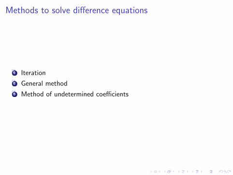
Methods to solve difference equations
1 Iteration
2 General method
3 Method of undetermined coefficients
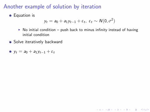
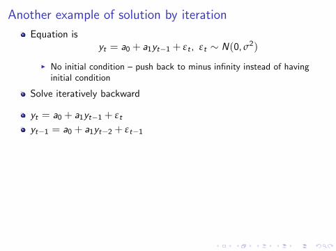
Another example of solution by iteration
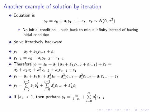
Equation isyt = a0 + a1yt−1 + εt , εt ∼ N(0, σ2)
I No initial condition – push back to minus infinity instead of havinginitial condition
Solve iteratively backward
yt = a0 + a1yt−1 + εt
yt−1 = a0 + a1yt−2 + εt−1Therefore yt = a0 + a1 (a0 + a1yt−2 + εt−1) + εt =a0 + a1a0 + a21yt−2 + a1εt−1 + εt
yt = a0 + a1a0 + a21a0 + a31yt−3 + a21εt−2 + a1εt−1 + εt
yt =t−1∑i=0
a0ai1 +
t−1∑i=0
ai1εt−i + at1y0
If |a1| < 1, then perhaps yt =a0
1−a1 +∞∑i=0
ai1εt−i
Cannot solve this way if a1 = 1 or |a1| > 1
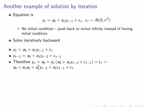
Another example of solution by iteration
Equation isyt = a0 + a1yt−1 + εt , εt ∼ N(0, σ2)
I No initial condition – push back to minus infinity instead of havinginitial condition
Solve iteratively backward
yt = a0 + a1yt−1 + εt
yt−1 = a0 + a1yt−2 + εt−1
Therefore yt = a0 + a1 (a0 + a1yt−2 + εt−1) + εt =a0 + a1a0 + a21yt−2 + a1εt−1 + εt
yt = a0 + a1a0 + a21a0 + a31yt−3 + a21εt−2 + a1εt−1 + εt
yt =t−1∑i=0
a0ai1 +
t−1∑i=0
ai1εt−i + at1y0
If |a1| < 1, then perhaps yt =a0
1−a1 +∞∑i=0
ai1εt−i
Cannot solve this way if a1 = 1 or |a1| > 1
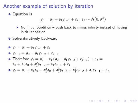
Another example of solution by iteration
Equation isyt = a0 + a1yt−1 + εt , εt ∼ N(0, σ2)
I No initial condition – push back to minus infinity instead of havinginitial condition
Solve iteratively backward
yt = a0 + a1yt−1 + εt
yt−1 = a0 + a1yt−2 + εt−1Therefore yt = a0 + a1 (a0 + a1yt−2 + εt−1) + εt =a0 + a1a0 + a21yt−2 + a1εt−1 + εt
yt = a0 + a1a0 + a21a0 + a31yt−3 + a21εt−2 + a1εt−1 + εt
yt =t−1∑i=0
a0ai1 +
t−1∑i=0
ai1εt−i + at1y0
If |a1| < 1, then perhaps yt =a0
1−a1 +∞∑i=0
ai1εt−i
Cannot solve this way if a1 = 1 or |a1| > 1
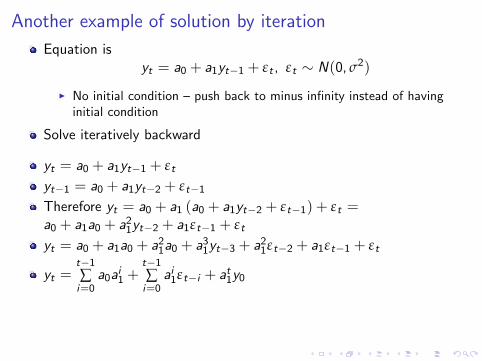
Another example of solution by iteration
Equation isyt = a0 + a1yt−1 + εt , εt ∼ N(0, σ2)
I No initial condition – push back to minus infinity instead of havinginitial condition
Solve iteratively backward
yt = a0 + a1yt−1 + εt
yt−1 = a0 + a1yt−2 + εt−1Therefore yt = a0 + a1 (a0 + a1yt−2 + εt−1) + εt =a0 + a1a0 + a21yt−2 + a1εt−1 + εt
yt = a0 + a1a0 + a21a0 + a31yt−3 + a21εt−2 + a1εt−1 + εt
yt =t−1∑i=0
a0ai1 +
t−1∑i=0
ai1εt−i + at1y0
If |a1| < 1, then perhaps yt =a0
1−a1 +∞∑i=0
ai1εt−i
Cannot solve this way if a1 = 1 or |a1| > 1
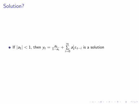
Solution?
If |a1| < 1, then yt =a0
1−a1 +∞∑i=0
ai1εt−i is a solution

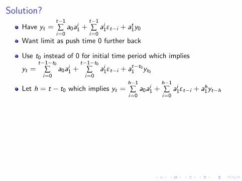
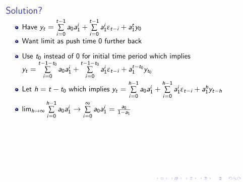
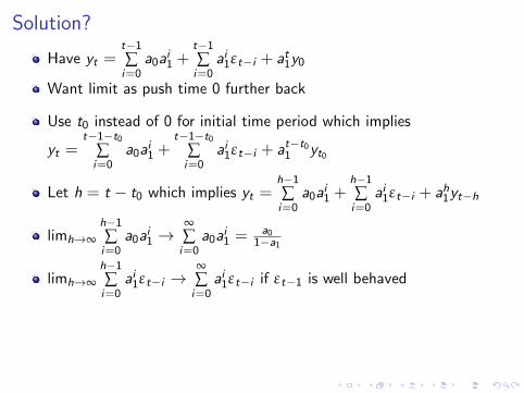
Solution?
Have yt =t−1∑i=0
a0ai1 +
t−1∑i=0
ai1εt−i + at1y0
Want limit as push time 0 further back
Use t0 instead of 0 for initial time period which implies
yt =t−1−t0
∑i=0
a0ai1 +
t−1−t0∑i=0
ai1εt−i + at−t01 yt0
Let h = t − t0 which implies yt =h−1∑i=0
a0ai1 +
h−1∑i=0
ai1εt−i + ah1yt−h
limh→∞h−1∑i=0
a0ai1 →
∞∑i=0
a0ai1 =
a01−a1
limh→∞h−1∑i=0
ai1εt−i →∞∑i=0
ai1εt−i if εt−1 is well behaved
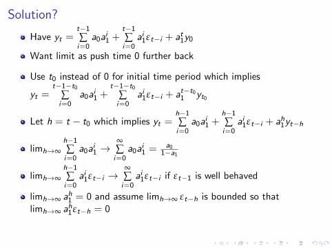
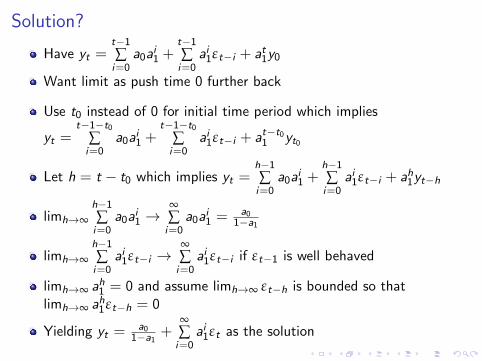
limh→∞ ah1 = 0 and assume limh→∞ εt−h is bounded so thatlimh→∞ ah1εt−h = 0
Yielding yt =a0
1−a1 +∞∑i=0
ai1εt as the solution
Solution?
Have yt =t−1∑i=0
a0ai1 +
t−1∑i=0
ai1εt−i + at1y0
Want limit as push time 0 further back
Use t0 instead of 0 for initial time period which implies
yt =t−1−t0
∑i=0
a0ai1 +
t−1−t0∑i=0
ai1εt−i + at−t01 yt0
Let h = t − t0 which implies yt =h−1∑i=0
a0ai1 +
h−1∑i=0
ai1εt−i + ah1yt−h
limh→∞h−1∑i=0
a0ai1 →
∞∑i=0
a0ai1 =
a01−a1
limh→∞h−1∑i=0
ai1εt−i →∞∑i=0
ai1εt−i if εt−1 is well behaved
limh→∞ ah1 = 0 and assume limh→∞ εt−h is bounded so thatlimh→∞ ah1εt−h = 0
Yielding yt =a0
1−a1 +∞∑i=0
ai1εt as the solution
General method of solution
Similar to way differential equations are solved
1 Solve the homogenous equation (no constant term)
2 Solve for a particular solution (complete equation)
3 The general solution is the sum of the particular solution and a linearcombination of all homogeneous solutions
4 There will be an arbitrary constant which can be eliminated byimposing the initial condition on the general solution or by driving thesolution back infinitely far
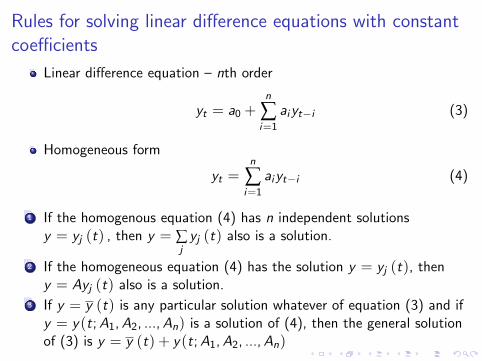
Rules for solving linear difference equations with constantcoefficients
Linear difference equation – nth order
yt = a0 +n
∑i=1
aiyt−i (3)
Homogeneous form
yt =n
∑i=1
aiyt−i (4)
1 If the homogenous equation (4) has n independent solutionsy = yj (t) , then y = ∑
jyj (t) also is a solution.
2 If the homogeneous equation (4) has the solution y = yj (t), theny = Ayj (t) also is a solution.
3 If y = y (t) is any particular solution whatever of equation (3) and ify = y(t;A1,A2, ...,An) is a solution of (4), then the general solutionof (3) is y = y (t) + y(t;A1,A2, ...,An)
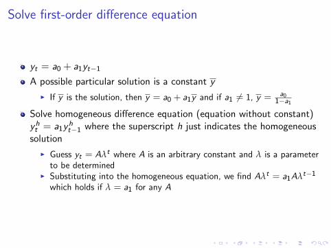
Solve first-order difference equation
yt = a0 + a1yt−1
A possible particular solution is a constant y
I If y is the solution, then y = a0 + a1y and if a1 6= 1, y = a01−a1
Solve homogeneous difference equation (equation without constant)yht = a1y
ht−1 where the superscript h just indicates the homogeneous
solution
I Guess yt = Aλt where A is an arbitrary constant and λ is a parameterto be determined
I Substituting into the homogeneous equation, we find Aλt = a1Aλt−1
which holds if λ = a1 for any A
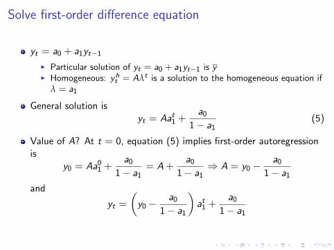
Solve first-order difference equation
yt = a0 + a1yt−1I Particular solution of yt = a0 + a1yt−1 is yI Homogeneous: yht = Aλt is a solution to the homogeneous equation if
λ = a1
General solution isyt = Aat1 +
a01− a1
(5)
Value of A? At t = 0, equation (5) implies first-order autoregressionis
y0 = Aa01 +a0
1− a1= A+
a01− a1
⇒ A = y0 −a0
1− a1
and
yt =
(y0 −
a01− a1
)at1 +
a01− a1
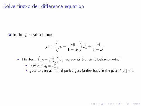
Solve first-order difference equation
In the general solution
yt =
(y0 −
a01− a1
)at1 +
a01− a1
I The term(y0 − a0
1−a1
)at1 represents transient behavior which
F is zero if y0 = a01−a1
F goes to zero as initial period gets farther back in the past if |a1| < 1
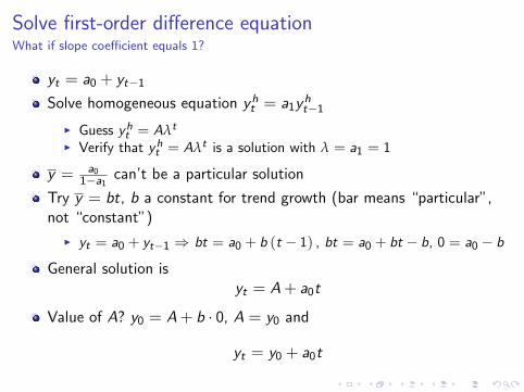
Solve first-order difference equationWhat if slope coefficient equals 1?
yt = a0 + yt−1
Solve homogeneous equation yht = a1yht−1
I Guess yht = Aλt
I Verify that yht = Aλt is a solution with λ = a1 = 1
y = a01−a1 can’t be a particular solution
Try y = bt, b a constant for trend growth (bar means “particular”,not “constant”)
I yt = a0 + yt−1 ⇒ bt = a0 + b (t − 1) , bt = a0 + bt − b, 0 = a0 − b
General solution isyt = A+ a0t
Value of A? y0 = A+ b · 0, A = y0 and
yt = y0 + a0t

Solve first-order difference equationWhat if slope coefficient is greater than 1?
yt = a0 + yt−1Solve homogeneous equation yht = a1y
ht−1
I Guess yht = Aλt
I Verify that yht = Aλt is a solution with λ = a1
y = a01−a1 can be a solution
I Verify that y = a01−a1 can be a solution
General solution isyt = Aat1 +
a01− a1
with the value of A set, it is
yt =
(y0 −
a01− a1
)at1 +
a01− a1
Transient behavior does not go to zeroI Becomes increasingly large as take initial period increasingly far back in
the past
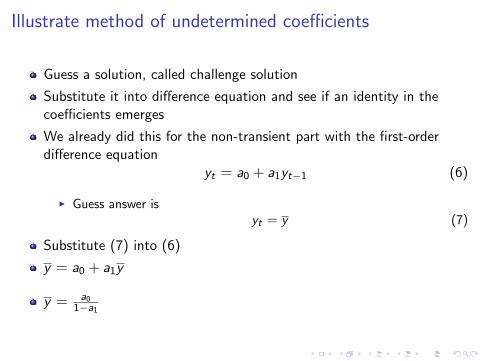
Illustrate method of undetermined coefficients
Guess a solution, called challenge solution
Substitute it into difference equation and see if an identity in thecoefficients emerges
We already did this for the non-transient part with the first-orderdifference equation
yt = a0 + a1yt−1 (6)
I Guess answer isyt = y (7)
Substitute (7) into (6)
y = a0 + a1y
y = a01−a1
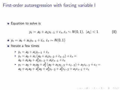
First-order autoregression with forcing variable I
Equation to solve is
yt = a0 + a1yt−1 + εt , εt ∼ N(0, 1), |a1| < 1 (8)
yt = a0 + a1yt−1 + εt , εt ∼ N(0, 1)
Iterate a few times
I yt = a0 + a1yt−1 + εtI yt = a0 + a1 (a0 + a1yt−2 + εt−1) + εt =
a0 + a1a0 + a21yt−2 + a1εt−1 + εtI yt = a0 + a1a0 + a21 (a0 + a1yt−3 + εt−2) + a1εt−1 + εt =
a0 + a1a0 + a21a0 + a31yt−3 + a21εt−2 + a1εt−1 + εt
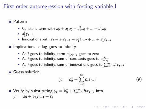
First-order autoregression with forcing variable I
Pattern
I Constant term with a0 + a1a0 + a21a0 + ... + ai1a0I ai1yt−iI Innovations with εt + a1εt−1 + a21εt−2 + ... + ai1εt−i
Implications as lag goes to infinity
I As i goes to infinity, term ai1yt−i goes to zeroI As i goes to infinity, sum of constants goes to a0
1−a1I As i goes to infinity, sum of innovations goes to ∑∞
i=0 ai1εt−i
Guess solution
yt = b∗0 +∞
∑i=0
bi εt−i (9)
Verify by substituting yt = b∗0 + ∑∞i=0 bi εt−i into
yt = a0 + a1yt−1 + εt
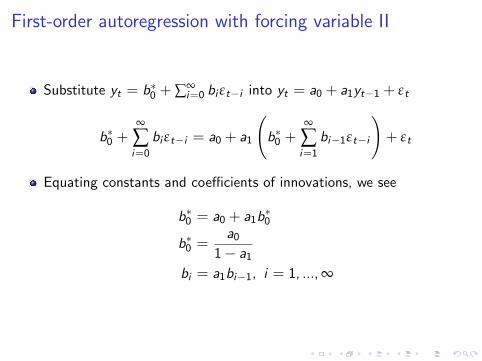
First-order autoregression with forcing variable II
Substitute yt = b∗0 + ∑∞i=0 bi εt−i into yt = a0 + a1yt−1 + εt
b∗0 +∞
∑i=0
bi εt−i = a0 + a1
(b∗0 +
∞
∑i=1
bi−1εt−i
)+ εt
Equating constants and coefficients of innovations, we see
b∗0 = a0 + a1b∗0
b∗0 =a0
1− a1bi = a1bi−1, i = 1, ..., ∞
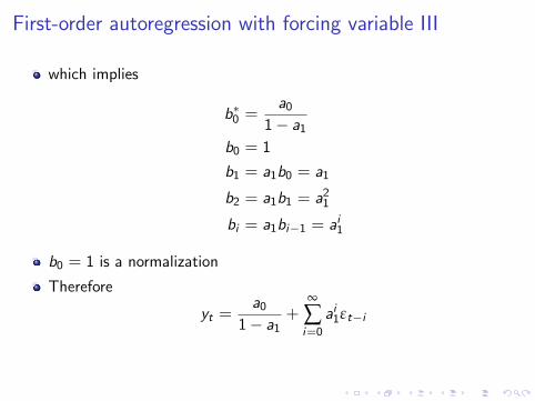
First-order autoregression with forcing variable III
which implies
b∗0 =a0
1− a1b0 = 1
b1 = a1b0 = a1
b2 = a1b1 = a21
bi = a1bi−1 = ai1
b0 = 1 is a normalization
Therefore
yt =a0
1− a1+
∞
∑i=0
ai1εt−i
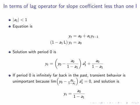
In terms of lag operator for slope coefficient less than one I
|a1| < 1
Equation is
yt = a0 + a1yt−1
(1− a1 L) yt = a0
Solution with period 0 is
yt =
(y0 −
a01− a1
)at1 +
a01− a1
If period 0 is infinitely far back in the past, transient behavior is
unimportant because lim(y0 − a0
1−a1
)at1 = 0, and solution is
yt =a0
1− a1
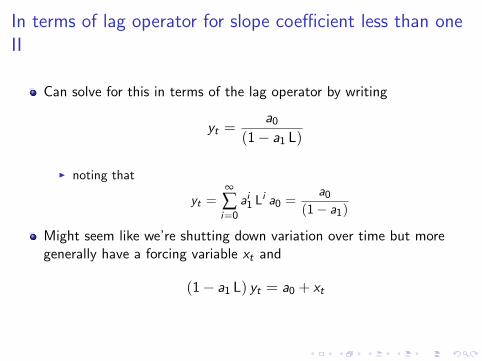
In terms of lag operator for slope coefficient less than oneII
Can solve for this in terms of the lag operator by writing
yt =a0
(1− a1 L)
I noting that
yt =∞
∑i=0
ai1 Li a0 =a0
(1− a1)
Might seem like we’re shutting down variation over time but moregenerally have a forcing variable xt and
(1− a1 L) yt = a0 + xt
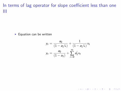
In terms of lag operator for slope coefficient less than oneIII
I Equation can be written
yt =a0
(1− a1 L)+
1
(1− a1 L)xt
yt =a0
(1− a1)+
∞
∑i=0
ai1xt
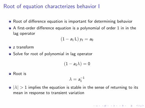
Root of equation characterizes behavior I
Root of difference equation is important for determining behavior
A first-order difference equation is a polynomial of order 1 in in thelag operator
(1− a1 L) yt = a0
z transform
Solve for root of polynomial in lag operator
(1− a1λ) = 0
Root is
λ = a−11
|λ| > 1 implies the equation is stable in the sense of returning to itsmean in response to transient variation
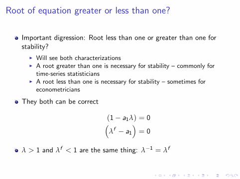
Root of equation greater or less than one?
Important digression: Root less than one or greater than one forstability?
I Will see both characterizationsI A root greater than one is necessary for stability – commonly for
time-series statisticiansI A root less than one is necessary for stability – sometimes for
econometricians
They both can be correct
(1− a1λ) = 0(λf − a1
)= 0
λ > 1 and λf < 1 are the same thing: λ−1 = λf
Possible strategy for solving difference equations I
Solve for roots in polynomial in lag operator or forward operator
We are interested in solving for roots to characterize behavior ofseries, not learning to be difference-equation wizards
Can rely on Fundamental theorem of algebra
I Every polynomial of order p has exactly p roots
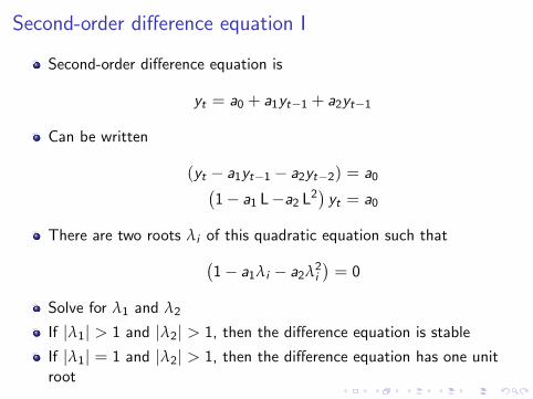
Second-order difference equation I
Second-order difference equation is
yt = a0 + a1yt−1 + a2yt−1
Can be written
(yt − a1yt−1 − a2yt−2) = a0(1− a1 L−a2 L2
)yt = a0
There are two roots λi of this quadratic equation such that(1− a1λi − a2λ2
i
)= 0
Solve for λ1 and λ2
If |λ1| > 1 and |λ2| > 1, then the difference equation is stable
If |λ1| = 1 and |λ2| > 1, then the difference equation has one unitroot
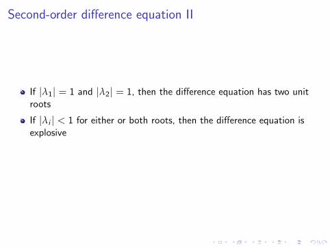
Second-order difference equation II
If |λ1| = 1 and |λ2| = 1, then the difference equation has two unitroots
If |λi | < 1 for either or both roots, then the difference equation isexplosive
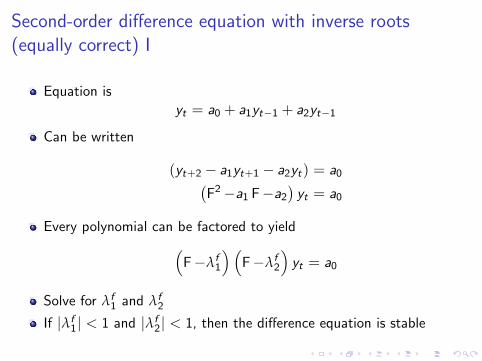
Second-order difference equation with inverse roots(equally correct) I
Equation is
yt = a0 + a1yt−1 + a2yt−1
Can be written
(yt+2 − a1yt+1 − a2yt) = a0(F2−a1 F−a2
)yt = a0
Every polynomial can be factored to yield(F−λf
1
) (F−λf
2
)yt = a0
Solve for λf1 and λf
2
If |λf1| < 1 and |λf
2| < 1, then the difference equation is stable
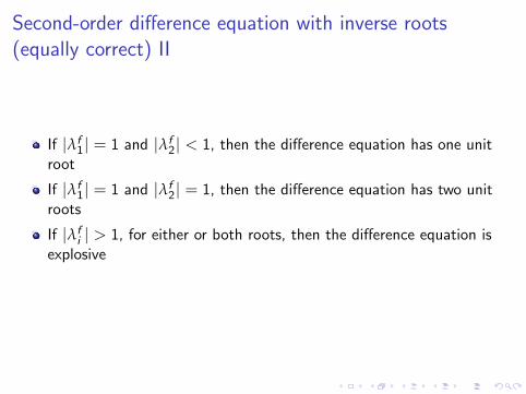
Second-order difference equation with inverse roots(equally correct) II
If |λf1| = 1 and |λf
2| < 1, then the difference equation has one unitroot
If |λf1| = 1 and |λf
2| = 1, then the difference equation has two unitroots
If |λfi | > 1, for either or both roots, then the difference equation is
explosive
Solving second-order difference equation I
We are interested in solving for roots to characterize behavior of timeseries, not to learn to be difference-equation wizards
Solve for roots of polynomial in lag operator or forward operator
Can rely on Fundamental theorem of algebra
I Every polynomial of order p has exactly p roots
General method
Equation isyt = a0 + a1yt−1 + a2yt−1
Can rely on Fundamental theorem of algebra
I Every polynomial of order p has exactly p rootsI That means two roots here
Particular solution
The particular solution is
y = a0 + a1y − a2y
andy =
a01− a1 + a2
if a1 + a2 6= 1
If a1 + a2 = 1, there is at least one unit root
Suppose there is no unit root
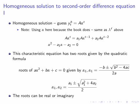
Homogeneous solution to second-order difference equationI
Homogeneous solution – guess yht = Aαt
I Note: Using α here because the book does – same as λf above
Aαt = a1Aαt−1 + a2Aαt−2
α2 − a1α− a2 = 0
This characteristic equation has two roots given by the quadraticformula
roots of aα2 + bα + c = 0 given by α1, α1 =−b±
√b2 − 4ac
2a
α1, α2 =a1 ±
√a21 + 4a2
2
The roots can be real or imaginary
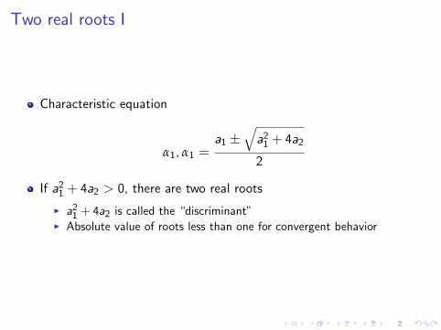
Two real roots I
Characteristic equation
α1, α1 =a1 ±
√a21 + 4a2
2
If a21 + 4a2 > 0, there are two real roots
I a21 + 4a2 is called the “discriminant”I Absolute value of roots less than one for convergent behavior

Discriminant is zero I
Characteristic equation
α1, α1 =a1 ±
√a21 + 4a2
2
If a21 + 4a2 = 0, it might seem there is only one root a1/2 but thereis another one
I The other root is t (a1/2) – a trend termI Probability of getting this with data is basically zero and I will move on
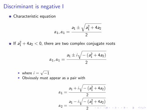
Discriminant is negative I
Characteristic equation
α1, α1 =a1 ±
√a21 + 4a2
2
If a21 + 4a2 < 0, there are two complex conjugate roots
α1, α1 =a1 ± i
√− (a21 + 4a2)
2
I where i =√−1
I Obviously must appear as a pair with
α1 =a1 + i
√−(a21 + 4a2
)2
α2 =a1 − i
√−(a21 + 4a2
)2
Discriminant is negative II
I Oscillatory behaviorI Can be stable or unstableI How can we tell? The unit circle
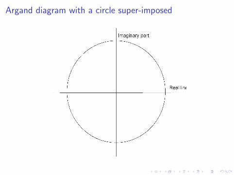
Argand diagram with a circle super-imposed
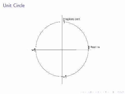
Unit Circle
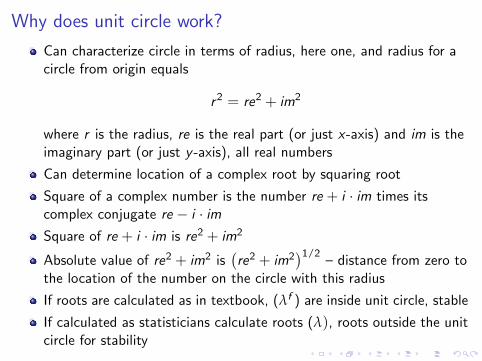
Why does unit circle work?
Can characterize circle in terms of radius, here one, and radius for acircle from origin equals
r2 = re2 + im2
where r is the radius, re is the real part (or just x-axis) and im is theimaginary part (or just y -axis), all real numbers
Can determine location of a complex root by squaring root
Square of a complex number is the number re + i · im times itscomplex conjugate re − i · imSquare of re + i · im is re2 + im2
Absolute value of re2 + im2 is(re2 + im2
)1/2– distance from zero to
the location of the number on the circle with this radius
If roots are calculated as in textbook, (λf ) are inside unit circle, stable
If calculated as statisticians calculate roots (λ), roots outside the unitcircle for stability
Complex roots and oscillations
Complex roots can be associated with oscillations – recurrent cycles
Can be seen through relationship of complex numbers and Arganddiagram
Simple way: spreadsheet
Summary
Difference equations can be stable or unstable
I Unstable means a trajectory that divergesI Stable means a trajectory that converges to a mean, to trend growth,
oscillations, some long-run path that could be repeated forever
The roots of a difference equation summarize the behavior
I As typically calculated by economists, roots with an absolute value lessthan one are stable
Second-order difference equations have two roots
I The roots can be complex numbersI Even so, roots with an absolute value less than one are stability
Unit roots mean the equation does not converge to a constant mean
Unit roots do not mean the equation is “unstable” in the sense ofdiverging from trend behavior
I yt = a0 + yt−1 always has the value given by yt − yt−1 = a0I Stable in terms of growth, just not level


![11.[36-49]Solution of a Subclass of Lane Emden Differential Equation by Variational Iteration Method](https://static.fdocuments.net/doc/165x107/577d1e5a1a28ab4e1e8e5546/1136-49solution-of-a-subclass-of-lane-emden-differential-equation-by-variational.jpg)