January 2013 Agenda Item X - Meeting Agendas (CA … · Web viewStudents learn to anticipate the...

California Department of Education i |March 2013

Common Core State Standards for Mathematicsfor California Public Schools

High School: Integrated Pathway Courses

Adopted by the California State Board of Education August 2010Updated January 2013Prepublication Version

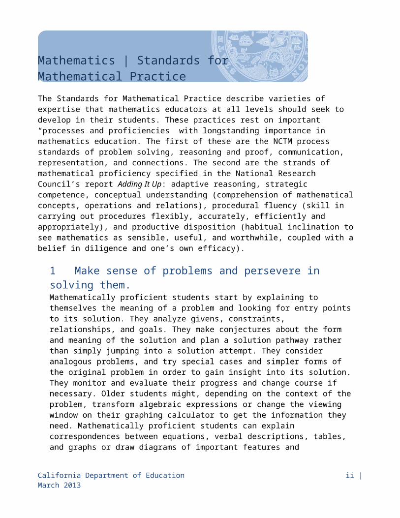
Mathematics | Standards for Mathematical PracticeThe Standards for Mathematical Practice describe varieties of expertise that mathematics educators at all levels should seek to develop in their students. These practices rest on important “processes and proficiencies” with longstanding importance in mathematics education. The first of these are the NCTM process standards of problem solving, reasoning and proof, communication, representation, and connections. The second are the strands of mathematical proficiency specified in the National Research Council’s report Adding It Up: adaptive reasoning, strategic competence, conceptual understanding (comprehension of mathematical concepts, operations and relations), procedural fluency (skill in carrying out procedures flexibly, accurately, efficiently and appropriately), and productive disposition (habitual inclination to see mathematics as sensible, useful, and worthwhile, coupled with a belief in diligence and one’s own efficacy).

1 Make sense of problems and persevere in solving them.Mathematically proficient students start by explaining to themselves the meaning of a problem and looking for entry points to its solution. They analyze givens, constraints, relationships, and goals. They make conjectures about the form and meaning of the solution and plan a solution pathway rather than simply jumping into a solution attempt. They consider analogous problems, and try special cases and simpler forms of the original problem in order to gain insight into its solution. They monitor and evaluate their progress and change course if necessary. Older students might, depending on the context of the problem, transform algebraic expressions or change the viewing window on their graphing calculator to get the information they need. Mathematically proficient students can explain correspondences between equations, verbal descriptions, tables, and graphs or draw diagrams of important features and relationships, graph data, and search for regularity or trends. Younger students might rely on using concrete objects or pictures to help conceptualize and solve a problem. Mathematically proficient students check their answers to problems using a different method, and they continually ask themselves, “Does this make sense?” They can understand the approaches of others to solving complex problems and identify correspondences between different approaches.

2 Reason abstractly and quantitatively.Mathematically proficient students make sense of quantities and their relationships in problem situations. They bring two complementary abilities to bear on problems involving quantitative relationships: the ability to decontextualize—to abstract a given situation and represent it symbolically and manipulate the representing symbols as if they have a life of their own, without necessarily attending to their referents—and the ability to contextualize, to pause as needed during the manipulation process in order to probe into the referents for the symbols involved. Quantitative reasoning entails habits of creating a coherent representation of the

California Department of Education ii |March 2013

problem at hand; considering the units involved; attending to the meaning of quantities, not just how to compute them; and knowing and flexibly using different properties of operations and objects.

3 Construct viable arguments and critique the reasoning of others.Mathematically proficient students understand and use stated assumptions, definitions, and previously established results in constructing arguments. They make conjectures and build a logical progression of statements to explore the truth of their conjectures. They are able to analyze situations by breaking them into cases, and can recognize and use counterexamples. They justify their conclusions, communicate them to others, and respond to the arguments of others. They reason inductively about data, making plausible arguments that take into account the context from which the data arose. Mathematically proficient students are also able to compare the effectiveness of two plausible arguments, distinguish correct logic or reasoning from that which is flawed, and—if there is a flaw in an argument—explain what it is. Elementary students can construct arguments using concrete referents such as objects, drawings, diagrams, and actions. Such arguments can make sense and be correct, even though they are not generalized or made formal until later grades. Later, students learn to determine domains to which an argument applies. Students at all grades can listen or read the arguments of others, decide whether they make sense, and ask useful questions to clarify or improve the arguments. Students build proofs by induction and proofs by contradiction. CA 3.1 (for higher mathematics only).

4 Model with mathematics.Mathematically proficient students can apply the mathematics they know to solve problems arising in everyday life, society, and the workplace. In early grades, this might be as simple as writing an addition equation to describe a situation. In middle grades, a student might apply proportional reasoning to plan a school event or analyze a problem in the community. By high school, a student might use geometry to solve a design problem or use a function to describe how one quantity of interest depends on another. Mathematically proficient students who can apply what they know are comfortable making assumptions and approximations to simplify a complicated situation, realizing that these may need revision later. They are able to identify important quantities in a practical situation and map their relationships using such tools as diagrams, two-way tables, graphs, flowcharts and formulas. They can analyze those relationships mathematically to draw conclusions. They routinely interpret their mathematical results in the context of the situation and reflect on whether the results make sense, possibly improving the model if it has not served its purpose.

5 Use appropriate tools strategically.Mathematically proficient students consider the available tools when solving a mathematical problem. These tools might include pencil and paper, concrete models, a ruler, a protractor, a calculator, a spreadsheet, a computer algebra system, a statistical package, or dynamic geometry software. Proficient students are sufficiently familiar with tools appropriate for their

California Department of Education iii |March 2013

grade or course to make sound decisions about when each of these tools might be helpful, recognizing both the insight to be gained and their limitations. For example, mathematically proficient high school students analyze graphs of functions and solutions generated using a graphing calculator. They detect possible errors by strategically using estimation and other mathematical knowledge. When making mathematical models, they know that technology can enable them to visualize the results of varying assumptions, explore consequences, and compare predictions with data. Mathematically proficient students at various grade levels are able to identify relevant external mathematical resources, such as digital content located on a website, and use them to pose or solve problems. They are able to use technological tools to explore and deepen their understanding of concepts.

6 Attend to precision.Mathematically proficient students try to communicate precisely to others. They try to use clear definitions in discussion with others and in their own reasoning. They state the meaning of the symbols they choose, including using the equal sign consistently and appropriately. They are careful about specifying units of measure, and labeling axes to clarify the correspondence with quantities in a problem. They calculate accurately and efficiently, express numerical answers with a degree of precision appropriate for the problem context. In the elementary grades, students give carefully formulated explanations to each other. By the time they reach high school they have learned to examine claims and make explicit use of definitions.

7 Look for and make use of structure.Mathematically proficient students look closely to discern a pattern or structure. Young students, for example, might notice that three and seven more is the same amount as seven and three more, or they may sort a collection of shapes according to how many sides the shapes have. Later, students will see 7 x 8 equals the well-remembered 7 x 5 + 7 x 3, in preparation for learning about the distributive property. In the expression x2 + 9x + 14, older students can see the 14 as 2 x 7 and the 9 as 2 + 7. They recognize the significance of an existing line in a geometric figure and can use the strategy of drawing an auxiliary line for solving problems. They also can step back for an overview and shift perspective. They can see complicated things, such as some algebraic expressions, as single objects or as being composed of several objects. For example, they can see 5 – 3(x – y)2 as 5 minus a positive number times a square and use that to realize that its value cannot be more than 5 for any real numbers x and y.

8 Look for and express regularity in repeated reasoning.Mathematically proficient students notice if calculations are repeated, and look both for general methods and for shortcuts. Upper elementary students might notice when dividing 25 by 11 that they are repeating the same calculations over and over again, and conclude they have a repeating decimal. By paying attention to the calculation of slope as they repeatedly check whether points are on the line through (1, 2) with slope 3, middle school students might abstract the equation (y – 2)/(x – 1) = 3. Noticing the regularity in the way terms cancel when expanding (x – 1)(x + 1), (x – 1)(x2 + x + 1), and (x – 1)(x3 + x2 + x + 1) might lead them to the

California Department of Education iv |March 2013

general formula for the sum of a geometric series. As they work to solve a problem, mathematically proficient students maintain oversight of the process, while attending to the details. They continually evaluate the reasonableness of their intermediate results.

California Department of Education v |March 2013

Higher Mathematics Standards

California Department of Education vi |March 2013

Standards for Higher MathematicsThe standards for higher mathematics are organized in two ways, as model courses and in conceptual categories, and include California additions1. The model courses consist of three courses in the traditional pathway (Algebra I, Geometry, and Algebra II); three courses in the integrated pathway (Mathematics I, II, and III); and two advanced courses (advanced Placement Statistics and Probability and Calculus). The model courses provide guidance for developing curriculum and instruction. The forthcoming Mathematics Framework for California Public Schools, Kindergarten Through Grade Twelve, will offer expanded explanations of the model courses and suggestions for additional courses, including Pre-Calculus and Statistics and Probability.

The six conceptual categories are number and quantity, algebra, functions, modeling, geometry, and statistics and probability. Conceptual categories portray a coherent view of higher mathematics and cross traditional course boundaries. There are no standards listed in the conceptual category of modeling. Instead, specific modeling standards appear throughout the other conceptual categories and are indicated by a star symbol ().

The higher mathematics standards specify the mathematics that all students should study in order to be college and career ready. Additional mathematics that students should learn in preparation for advanced courses, such as calculus, advanced statistics, or discrete mathematics, is indicated by (+). All standards without a (+) symbol should be in the common mathematics curriculum for all college and career ready students. Standards with a (+) symbol may also appear in courses intended for all students.

1 California additions appear in bold type and with a CA notation.

California Department of Education vii |March 2013

Table 1: Model Mathematics Courses, by Grade Level (see above paragraph for explanation of table below)

Discipline GradeSeven

GradeEight

GradeNine

GradeTen

GradeEleven

GradeTwelve

Algebra I/Mathematics I 7th 8th 9th 10th 11th 12th

Geometry/Mathematics II 8th 9th 10th 11th 12th

Algebra II/Mathematics III 9th 10th 11th 12th

Advanced Placement Probability and Statistics 10th 11th 12th

Calculus 10th 11th 12th

Local districts determine which course offerings and sequences best meet the needs of their students. The table above provides guidance on possible course-taking sequences in higher mathematics. It is not intended to be an exhaustive list of courses or sequences of courses that students could take. In the forthcoming Mathematics Framework for California Public Schools, Kindergarten Through Grade Twelve, courses in Pre-Calculus and Statistics and Probability will also be presented.

California Department of Education viii |March 2013

Higher

Mathematics Courses

California Department of Education ix |March 2013

Integrated Pathway

Mathematics I Introduction1

The fundamental purpose of the Model Mathematics I course is to formalize and extend the mathematics that students learned in the middle grades. This course is comprised of standards selected from the high school conceptual categories, which were written to encompass the scope of content and skills to be addressed throughout grades 9–12 rather than through any single course. Therefore, the complete standard is presented in the model course, with clarifying footnotes as needed to limit the scope of the standard and indicate what is appropriate for study in this particular course. For example, the scope of Model Mathematics I is limited to linear and exponential expressions and functions as well as some work with absolute value, step, and functions that are piecewise-defined. Therefore, although a standard may include references to quadratic, logarithmic, or trigonometric functions, those functions should not be included in coursework for Model Mathematics I; they will be addressed in Model Mathematics II or III.

For the high school Model Mathematics I course, instructional time should focus on six critical areas, each of which is described in more detail below: (1) extend understanding of numerical manipulation to algebraic manipulation; (2) synthesize understanding of function; (3) deepen and extend understanding of linear relationships; (4) apply linear models to data that exhibit a linear trend; (5) establish criteria for congruence based on rigid motions; and (6) apply the Pythagorean Theorem to the coordinate plane.

(1) By the end of eighth grade students have had a variety of experiences working with expressions and creating equations. Students become facile with algebraic manipulation in much the same way that they are facile with numerical manipulation. Algebraic facility includes rearranging and collecting terms, factoring, identifying and canceling common factors in rational expressions, and applying properties of exponents. Students continue this work by using quantities to model and analyze situations, to interpret expressions, and to create equations to describe situations.

(2) In earlier grades, students define, evaluate, and compare functions, and use them to model relationships among quantities. Students will learn function notation and develop the concepts of domain and range. They move beyond viewing functions as processes that take inputs and yield outputs and start viewing functions as objects in their own right. They explore many examples of functions, including sequences; interpret functions given graphically, numerically, symbolically, and verbally; translate between representations; and understand the limitations of various representations. They work with functions given by graphs and tables, keeping in mind that, depending upon the context, these representations are likely to be approximate and incomplete. Their work includes

1 Massachusetts Department of Elementary and Secondary Education, Massachusetts Curriculum Framework for Mathematics, 2011, p. 129–130.

California Department of Education x |March 2013

Mathematics I Introduction functions that can be described or approximated by formulas as well as those that cannot. When functions describe relationships between quantities arising from a context, students reason with the units in which those quantities are measured. Students build on and informally extend their understanding of integer exponents to consider exponential functions. They compare and contrast linear and exponential functions, distinguishing between additive and multiplicative change. They interpret arithmetic sequences as linear functions and geometric sequences as exponential functions.

(3) By the end of eighth grade, students have learned to solve linear equations in one variable and have applied graphical and algebraic methods to analyze and solve systems of linear equations in two variables. Building on these earlier experiences, students analyze and explain the process of solving an equation, and justify the process used in solving a system of equations. Students develop fluency writing, interpreting, and translating among various forms of linear equations and inequalities, and use them to solve problems. They master the solution of linear equations and apply related solution techniques and the laws of exponents to the creation and solution of simple exponential equations. Students explore systems of equations and inequalities, and they find and interpret their solutions. All of this work is grounded on understanding quantities and on relationships among them.

(4) Students’ prior experiences with data are the basis for the more formal means of assessing how a model fits data. Students use regression techniques to describe approximately linear relationships among quantities. They use graphical representations and knowledge of the context to make judgments about the appropriateness of linear models. With linear models, they look at residuals to analyze the goodness of fit.

(5) In previous grades, students were asked to draw triangles based on given measurements. They also have prior experience with rigid motions: translations, reflections, and rotations, and have used these to develop notions about what it means for two objects to be congruent. Students establish triangle congruence criteria, based on analyses of rigid motions and formal constructions. They solve problems about triangles, quadrilaterals, and other polygons. They apply reasoning to complete geometric constructions and explain why they work.

(6) Building on their work with the Pythagorean Theorem in eighth grade to find distances, students use a rectangular coordinate system to verify geometric relationships, including properties of special triangles and quadrilaterals and slopes of parallel and perpendicular lines.

The Standards for Mathematical Practice complement the content standards so that students increasingly engage with the subject matter as they grow in mathematical maturity and expertise throughout the elementary, middle, and high school years.

California Department of Education xi |March 2013

M1

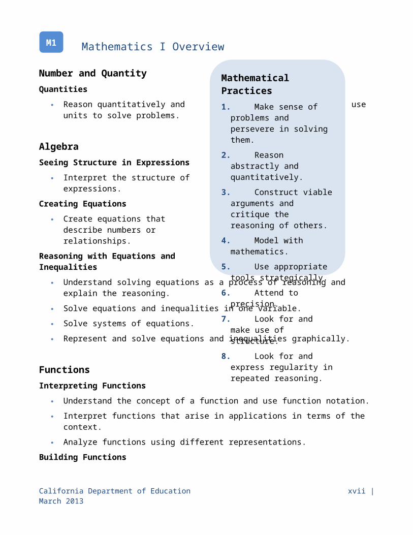
Mathematics I OverviewNumber and QuantityQuantities

Reason quantitatively and use units to solve problems.

AlgebraSeeing Structure in Expressions

Interpret the structure of expressions.

Creating Equations

Create equations that describe numbers or relationships.

Reasoning with Equations and Inequalities

Understand solving equations as a process of reasoning and explain the reasoning.

Solve equations and inequalities in one variable.

Solve systems of equations.

Represent and solve equations and inequalities graphically.

FunctionsInterpreting Functions

Understand the concept of a function and use function notation.

Interpret functions that arise in applications in terms of the context.

Analyze functions using different representations.

Building Functions

Build a function that models a relationship between two quantities.

Build new functions from existing functions.

Linear, Quadratic, and Exponential Models

Construct and compare linear, quadratic, and exponential models and solve problems.

Interpret expressions for functions in terms of the situation they model.

California Department of Education xii |March 2013

M1

Mathematical Practices1. Make sense of

problems and persevere in solving them.

2. Reason abstractly and quantitatively.

3. Construct viable arguments and critique the reasoning of others.

4. Model with mathematics.

5. Use appropriate tools strategically.

6. Attend to precision.

7. Look for and make use of structure.

8. Look for and express regularity in repeated reasoning.

Mathematics I Overview GeometryCongruence

Experiment with transformations in the plane.

Understand congruence in terms of rigid motions.

Make geometric constructions.

Expressing Geometric Properties with Equations

Use coordinates to prove simple geometric theorems algebraically.

Statistics and ProbabilityInterpreting Categorical and Quantitative Data

Summarize, represent, and interpret data on a single count or measurement variable.

Summarize, represent, and interpret data on two categorical and quantitative variables.

Interpret linear models

Indicates a modeling standard linking mathematics to everyday life, work, and decision-making(+) Indicates additional mathematics to prepare students for advanced courses

California Department of Education xiii |March 2013

M1

Mathematics I

Number and Quantity

Quantities N-QReason quantitatively and use units to solve problems. [Foundation for work with expressions, equations and functions.]

1. Use units as a way to understand problems and to guide the solution of multi-step problems; choose and interpret units consistently in formulas; choose and interpret the scale and the origin in graphs and data displays.

2. Define appropriate quantities for the purpose of descriptive modeling. 3. Choose a level of accuracy appropriate to limitations on measurement when reporting quantities.

Algebra

Seeing Structure in Expressions A-SSEInterpret the structure of expressions. [Linear expressions and exponential expressions with integer exponents.]

1. Interpret expressions that represent a quantity in terms of its context. a. Interpret parts of an expression, such as terms, factors, and coefficients. b. Interpret complicated expressions by viewing one or more of their parts as a single entity. For

example, interpret P(1 + r)n as the product of P and a factor not depending on P.

Creating Equations A-CEDCreate equations that describe numbers or relationships. [Linear, and exponential (integer inputs only); for A.CED.3, linear only.]

1. Create equations and inequalities in one variable including ones with absolute value and use them to solve problems. Include equations arising from linear and quadratic functions, and simple rational and exponential functions. CA

2. Create equations in two or more variables to represent relationships between quantities; graph equations on coordinate axes with labels and scales.

3. Represent constraints by equations or inequalities, and by systems of equations and/or inequalities, and interpret solutions as viable or non-viable options in a modeling context. For example, represent inequalities describing nutritional and cost constraints on combinations of different foods.

4. Rearrange formulas to highlight a quantity of interest, using the same reasoning as in solving equations. For example, rearrange Ohm’s law V = IR to highlight resistance R.

Reasoning with Equations and Inequalities A-REIUnderstand solving equations as a process of reasoning and explain the reasoning. [Master linear, learn as general principle.]

1. Explain each step in solving a simple equation as following from the equality of numbers asserted at the previous step, starting from the assumption that the original equation has a solution. Construct a viable argument to justify a solution method.

California Department of Education xiv |March 2013

M1

Mathematics I Solve equations and inequalities in one variable.

3. Solve linear equations and inequalities in one variable, including equations with coefficients represented by letters. [Linear inequalities; literal equations that are linear in the variables being solved for; exponential of a form, such as 2x = 1/16.]

3.1 Solve one-variable equations and inequalities involving absolute value, graphing the solutions and interpreting them in context. CA

Solve systems of equations. [Linear systems.]5. Prove that, given a system of two equations in two variables, replacing one equation by the sum of that

equation and a multiple of the other produces a system with the same solutions. 6. Solve systems of linear equations exactly and approximately (e.g., with graphs), focusing on pairs of

linear equations in two variables.

Represent and solve equations and inequalities graphically. [Linear and exponential; learn as general principle.]10. Understand that the graph of an equation in two variables is the set of all its solutions plotted in the

coordinate plane, often forming a curve (which could be a line). 11. Explain why the x-coordinates of the points where the graphs of the equations y = f(x) and y = g(x)

intersect are the solutions of the equation f(x) = g(x); find the solutions approximately, e.g., using technology to graph the functions, make tables of values, or find successive approximations. Include cases where f(x) and/or g(x) are linear, polynomial, rational, absolute value, exponential, and logarithmic functions.

12. Graph the solutions to a linear inequality in two variables as a half-plane (excluding the boundary in the case of a strict inequality), and graph the solution set to a system of linear inequalities in two variables as the intersection of the corresponding half-planes.

Functions

Interpreting Functions F-IFUnderstand the concept of a function and use function notation. [Learn as general principle. Focus on linear and exponential (integer domains) and on arithmetic and geometric sequences.]

1. Understand that a function from one set (called the domain) to another set (called the range) assigns to each element of the domain exactly one element of the range. If f is a function and x is an element of its domain, then f(x) denotes the output of f corresponding to the input x. The graph of f is the graph of the equation y = f(x).

2. Use function notation, evaluate functions for inputs in their domains, and interpret statements that use function notation in terms of a context. ).

3. Recognize that sequences are functions, sometimes defined recursively, whose domain is a subset of the integers. For example, the Fibonacci sequence is defined recursively by f(0) = f(1) = 1, f(n + 1) = f(n) + f(n 1) for n ≥ 1. ).

Interpret functions that arise in applications in terms of the context. [Linear and exponential, (linear domain).]4. For a function that models a relationship between two quantities, interpret key features of graphs and

tables in terms of the quantities, and sketch graphs showing key features given a verbal description of the relationship. Key features include: intercepts; intervals where the function is increasing, decreasing, positive, or negative; relative maximums and minimums; symmetries; end behavior; and periodicity.

California Department of Education xv |March 2013

M1

Mathematics I 5. Relate the domain of a function to its graph and, where applicable, to the quantitative relationship it

describes. For example, if the function h gives the number of person-hours it takes to assemble n engines in a factory, then the positive integers would be an appropriate domain for the function.

6. Calculate and interpret the average rate of change of a function (presented symbolically or as a table) over a specified interval. Estimate the rate of change from a graph.

Analyze functions using different representations. [Linear and exponential.]7. Graph functions expressed symbolically and show key features of the graph, by hand in simple cases and

using technology for more complicated cases. a. Graph linear and quadratic functions and show intercepts, maxima, and minima. e. Graph exponential and logarithmic functions, showing intercepts and end behavior, and

trigonometric functions, showing period, midline, and amplitude. 9. Compare properties of two functions each represented in a different way (algebraically, graphically,

numerically in tables, or by verbal descriptions).

Building Functions F-BFBuild a function that models a relationship between two quantities. [For F.BF.1, 2, linear and exponential (integer inputs).]

1. Write a function that describes a relationship between two quantities. a. Determine an explicit expression, a recursive process, or steps for calculation from a context. b. Combine standard function types using arithmetic operations. For example, build a function that

models the temperature of a cooling body by adding a constant function to a decaying exponential, and relate these functions to the model.

2. Write arithmetic and geometric sequences both recursively and with an explicit formula, use them to model situations, and translate between the two forms.

Build new functions from existing functions. [Linear and exponential; focus on vertical translations for exponential.]3. Identify the effect on the graph of replacing f(x) by f(x) + k, kf(x), f(kx), and f(x + k) for specific values of k

(both positive and negative); find the value of k given the graphs. Experiment with cases and illustrate an explanation of the effects on the graph using technology. Include recognizing even and odd functions from their graphs and algebraic expressions for them.

Linear, Quadratic, and Exponential Models F-LEConstruct and compare linear, quadratic, and exponential models and solve problems. [Linear and exponential.]

1. Distinguish between situations that can be modeled with linear functions and with exponential functions.

a. Prove that linear functions grow by equal differences over equal intervals, and that exponential functions grow by equal factors over equal intervals.

b. Recognize situations in which one quantity changes at a constant rate per unit interval relative to another.

c. Recognize situations in which a quantity grows or decays by a constant percent rate per unit interval relative to another.

2. Construct linear and exponential functions, including arithmetic and geometric sequences, given a graph, a description of a relationship, or two input-output pairs (include reading these from a table).

California Department of Education xvi |March 2013

M1

Mathematics I 3. Observe using graphs and tables that a quantity increasing exponentially eventually exceeds a quantity

increasing linearly, quadratically, or (more generally) as a polynomial function.

Interpret expressions for functions in terms of the situation they model. [Linear and exponential of form f(x) = bx + k.]

5. Interpret the parameters in a linear or exponential function in terms of a context.

Geometry

Congruence G-COExperiment with transformations in the plane.

1. Know precise definitions of angle, circle, perpendicular line, parallel line, and line segment, based on the undefined notions of point, line, distance along a line, and distance around a circular arc.

2. Represent transformations in the plane using, e.g., transparencies and geometry software; describe transformations as functions that take points in the plane as inputs and give other points as outputs. Compare transformations that preserve distance and angle to those that do not (e.g., translation versus horizontal stretch).

3. Given a rectangle, parallelogram, trapezoid, or regular polygon, describe the rotations and reflections that carry it onto itself.

4. Develop definitions of rotations, reflections, and translations in terms of angles, circles, perpendicular lines, parallel lines, and line segments.

5. Given a geometric figure and a rotation, reflection, or translation, draw the transformed figure using, e.g., graph paper, tracing paper, or geometry software. Specify a sequence of transformations that will carry a given figure onto another.

Understand congruence in terms of rigid motions. [Build on rigid motions as a familiar starting point for development of concept of geometric proof.]

6. Use geometric descriptions of rigid motions to transform figures and to predict the effect of a given rigid motion on a given figure; given two figures, use the definition of congruence in terms of rigid motions to decide if they are congruent.

7. Use the definition of congruence in terms of rigid motions to show that two triangles are congruent if and only if corresponding pairs of sides and corresponding pairs of angles are congruent.

8. Explain how the criteria for triangle congruence (ASA, SAS, and SSS) follow from the definition of congruence in terms of rigid motions.

Make geometric constructions. [Formalize and explain processes.]12. Make formal geometric constructions with a variety of tools and methods (compass and straightedge,

string, reflective devices, paper folding, dynamic geometric software, etc.). Copying a segment; copying an angle; bisecting a segment; bisecting an angle; constructing perpendicular lines, including the perpendicular bisector of a line segment; and constructing a line parallel to a given line through a point not on the line.

13. Construct an equilateral triangle, a square, and a regular hexagon inscribed in a circle.

California Department of Education xvii |March 2013

M1

Mathematics I Geometry

Expressing Geometric Properties with Equations G-GPEUse coordinates to prove simple geometric theorems algebraically. [Include distance formula; relate to Pythagorean Theorem.]

4. Use coordinates to prove simple geometric theorems algebraically. 5. Prove the slope criteria for parallel and perpendicular lines and use them to solve geometric problems

(e.g., find the equation of a line parallel or perpendicular to a given line that passes through a given point).

7. Use coordinates to compute perimeters of polygons and areas of triangles and rectangles, e.g., using the distance formula.

Statistics and Probability

Interpreting Categorical and Quantitative Data S-IDSummarize, represent, and interpret data on a single count or measurement variable.

1. Represent data with plots on the real number line (dot plots, histograms, and box plots). 2. Use statistics appropriate to the shape of the data distribution to compare center (median, mean) and

spread (interquartile range, standard deviation) of two or more different data sets. 3. Interpret differences in shape, center, and spread in the context of the data sets, accounting for possible

effects of extreme data points (outliers).

Summarize, represent, and interpret data on two categorical and quantitative variables. [Linear focus; discuss general principle.]

5. Summarize categorical data for two categories in two-way frequency tables. Interpret relative frequencies in the context of the data (including joint, marginal, and conditional relative frequencies). Recognize possible associations and trends in the data.

6. Represent data on two quantitative variables on a scatter plot, and describe how the variables are related.

a. Fit a function to the data; use functions fitted to data to solve problems in the context of the data. Use given functions or choose a function suggested by the context. Emphasize linear, quadratic, and exponential models.

b. Informally assess the fit of a function by plotting and analyzing residuals. c. Fit a linear function for a scatter plot that suggests a linear association.

Interpret linear models. 7. Interpret the slope (rate of change) and the intercept (constant term) of a linear model in the context of

the data. 8. Compute (using technology) and interpret the correlation coefficient of a linear fit. 9. Distinguish between correlation and causation.

California Department of Education xviii |March 2013

M1

Mathematics II Introduction1

The focus of the Model Mathematics II course is on quadratic expressions, equations, and functions; comparing their characteristics and behavior to those of linear and exponential relationships from Model Mathematics I. This course is comprised of standards selected from the high school conceptual categories, which were written to encompass the scope of content and skills to be addressed throughout grades 9–12 rather than through any single course. Therefore, the complete standard is presented in the model course, with clarifying footnotes as needed to limit the scope of the standard and indicate what is appropriate for study in this particular course. For example, the scope of Model Mathematics II is limited to quadratic expressions and functions, and some work with absolute value, step, and functions that are piecewise-defined. Therefore, although a standard may include references to logarithms or trigonometry, those functions should not be included in coursework for Model Mathematics II; they will be addressed in Model Mathematics III.

For the high school Model Mathematics II course, instructional time should focus on five critical areas: (1) extend the laws of exponents to rational exponents; (2) compare key characteristics of quadratic functions with those of linear and exponential functions; (3) create and solve equations and inequalities involving linear, exponential, and quadratic expressions; (4) extend work with probability; and (5) establish criteria for similarity of triangles based on dilations and proportional reasoning.

(1) Students extend the laws of exponents to rational exponents and explore distinctions between rational and irrational numbers by considering their decimal representations. Students learn that when quadratic equations do not have real solutions, the number system must be extended so that solutions exist, analogous to the way in which extending the whole numbers to the negative numbers allows x + 1 = 0 to have a solution. Students explore relationships between number systems: whole numbers, integers, rational numbers, real numbers, and complex numbers. The guiding principle is that equations with no solutions in one number system may have solutions in a larger number system.

(2) Students consider quadratic functions, comparing the key characteristics of quadratic functions to those of linear and exponential functions. They select from among these functions to model phenomena. Students learn to anticipate the graph of a quadratic function by interpreting various forms of quadratic expressions. In particular, they identify the real solutions of a quadratic equation as the zeros of a related quadratic function. When quadratic equations do not have real solutions, students learn that that the graph of the related quadratic function does not cross the horizontal axis. They expand their


California Department of Education xix |March 2013

Mathematics II Introductionexperience with functions to include more specialized functions—absolute value, step, and those that are piecewise-defined.

(3) Students begin by focusing on the structure of expressions, rewriting expressions to clarify and reveal aspects of the relationship they represent. They create and solve equations, inequalities, and systems of equations involving exponential and quadratic expressions.

(4) Building on probability concepts that began in the middle grades, students use the language of set theory to expand their ability to compute and interpret theoretical and experimental probabilities for compound events, attending to mutually exclusive events, independent events, and conditional probability. Students should make use of geometric probability models wherever possible. They use probability to make informed decisions.

(5) Students apply their earlier experience with dilations and proportional reasoning to build a formal understanding of similarity. They identify criteria for similarity of triangles, use similarity to solve problems, and apply similarity in right triangles to understand right triangle trigonometry, with particular attention to special right triangles and the Pythagorean Theorem. Students develop facility with geometric proof. They use what they know about congruence and similarity to prove theorems involving lines, angles, triangles, and other polygons. They explore a variety of formats for writing proofs.


California Department of Education xx |March 2013

M2

Mathematics II Overview

Number and QuantityThe Real Number System

Extend the properties of exponents to rational exponents.

Use properties of rational and irrational numbers.The Complex Number Systems

Perform arithmetic operations with complex numbers.

Use complex numbers in polynomial identities and equations.


Interpret the structure of expressions. Write expressions in equivalent forms to solve

problems.Arithmetic with Polynomials and Rational Expressions

Perform arithmetic operations on polynomials.Creating Equations

Create equations that describe numbers or relationships.Reasoning with Equations and Inequalities

Solve equations and inequalities in one variable. Solve systems of equations.


Interpret functions that arise in applications in terms of the context. Analyze functions using different representations.

Building Functions Build a function that models a relationship between two quantities. Build new functions from existing functions.

Linear, Quadratic, and Exponential Models Construct and compare linear, quadratic and exponential models and solve problems. Interpret expressions for functions in terms of the situation they model.

California Department of Education xxi |March 2013

M2










Mathematics II OverviewTrigonometric Functions

Prove and apply trigonometric identities.

GeometryCongruence

Prove geometric theorems.Similarity, Right Triangles, and Trigonometry

Understand similarity in terms of similarity transformations. Prove theorems involving similarity. Define trigonometric ratios and solve problems involving right triangles.

Circles Understand and apply theorems about circles. Find arc lengths and areas of sectors of circles.

Expressing Geometric Properties with Equations Translate between the geometric description and the equation for a conic section. Use coordinates to prove simple geometric theorems algebraically.

Geometric Measurement and Dimension Explain volume formulas and use them to solve problems.

Statistics and ProbabilityConditional Probability and the Rules of Probability

Understand independence and conditional probability and use them to interpret data. Use the rules of probability to compute probabilities of compound events in a uniform

probability model.Using Probability to Make Decisions

Use probability to evaluate outcomes of decisions


California Department of Education xxii |March 2013

M2

Mathematics II Number and Quantity

The Real Number System N-RNExtend the properties of exponents to rational exponents.

1. Explain how the definition of the meaning of rational exponents follows from extending the properties of integer exponents to those values, allowing for a notation for radicals in terms of rational exponents. For example, we define 51/3 to be the cube root of 5 because we want (51/3)3 = 5(1/3)3 to hold, so (51/3)3 must equal 5.

2. Rewrite expressions involving radicals and rational exponents using the properties of exponents.

Use properties of rational and irrational numbers.3. Explain why the sum or product of two rational numbers is rational; that the sum of a rational number

and an irrational number is irrational; and that the product of a nonzero rational number and an irrational number is irrational.

The Complex Number System N-CNPerform arithmetic operations with complex numbers. [i2 as highest power of i.]

1. Know there is a complex number i such that

i 2 = −1, and every complex number has the form a + bi with a and b real.

2. Use the relation

i 2 = –1 and the commutative, associative, and distributive properties to add, subtract, and multiply complex numbers.

Use complex numbers in polynomial identities and equations. [Quadratics with real coefficients.]7. Solve quadratic equations with real coefficients that have complex solutions. 8. (+) Extend polynomial identities to the complex numbers. For example, rewrite x2 + 4 as (x + 2i)(x – 2i). 9. (+) Know the Fundamental Theorem of Algebra; show that it is true for quadratic polynomials.

Algebra

Seeing Structure in Expressions A-SSEInterpret the structure of expressions. [Quadratic and exponential.]

1. Interpret expressions that represent a quantity in terms of its context. a. Interpret parts of an expression, such as terms, factors, and coefficients. b. Interpret complicated expressions by viewing one or more of their parts as a single entity. For

example, interpret P(1 + r)n as the product of P and a factor not depending on P.

2. Use the structure of an expression to identify ways to rewrite it. For example, see x4 – y4 as (x2)2 – (y2)2, thus recognizing it as a difference of squares that can be factored as (x2 – y2)(x2 + y2).

Write expressions in equivalent forms to solve problems. [Quadratic and exponential.]3. Choose and produce an equivalent form of an expression to reveal and explain properties of the quantity

represented by the expression. a. Factor a quadratic expression to reveal the zeros of the function it defines. b. Complete the square in a quadratic expression to reveal the maximum or minimum value of the

function it defines.

California Department of Education xxiii |March 2013

M2

Mathematics II c. Use the properties of exponents to transform expressions for exponential functions. For

example, the expression 1.15t can be rewritten as (1.151/12)12t ≈ 1.01212t to reveal the approximate equivalent monthly interest rate if the annual rate is 15%.

Arithmetic with Polynomials and Rational Expressions A-APRPerform arithmetic operations on polynomials. [Polynomials that simplify to quadratics.]

1. Understand that polynomials form a system analogous to the integers, namely, they are closed under the operations of addition, subtraction, and multiplication; add, subtract, and multiply polynomials.

Creating Equations A-CEDCreate equations that describe numbers or relationships.



4. Rearrange formulas to highlight a quantity of interest, using the same reasoning as in solving equations. [Include formulas involving quadratic terms.]

Reasoning with Equations and Inequalities A-REISolve equations and inequalities in one variable. [Quadratics with real coefficients.]

4. Solve quadratic equations in one variable. a. Use the method of completing the square to transform any quadratic equation in x into an

equation of the form (x – p)2 = q that has the same solutions. Derive the quadratic formula from this form.

b. Solve quadratic equations by inspection (e.g., for x2 = 49), taking square roots, completing the square, the quadratic formula, and factoring, as appropriate to the initial form of the equation. Recognize when the quadratic formula gives complex solutions and write them as a ± bi for real numbers a and b.

Solve systems of equations. [Linear-quadratic systems.]7. Solve a simple system consisting of a linear equation and a quadratic equation in two variables

algebraically and graphically. For example, find the points of intersection between the line y = –3x and the circle x2 + y2 = 3.

Functions

Interpreting Functions F-IFInterpret functions that arise in applications in terms of the context. [Quadratic.]

4. For a function that models a relationship between two quantities, interpret key features of graphs and tables in terms of the quantities, and sketch graphs showing key features given a verbal description of the relationship. Key features include: intercepts; intervals where the function is increasing, decreasing, positive, or negative; relative maximums and minimums; symmetries; end behavior; and periodicity.

California Department of Education xxiv |March 2013

M2

Mathematics II 5. Relate the domain of a function to its graph and, where applicable, to the quantitative relationship it

describes.6. Calculate and interpret the average rate of change of a function (presented symbolically or as a table)

over a specified interval. Estimate the rate of change from a graph.

Analyze functions using different representations. [Linear, exponential, quadratic, absolute value, step, piecewise-defined.]

7. Graph functions expressed symbolically and show key features of the graph, by hand in simple cases and using technology for more complicated cases.

a. Graph linear and quadratic functions and show intercepts, maxima, and minima. b. Graph square root, cube root, and piecewise-defined functions, including step functions and

absolute value functions. 8. Write a function defined by an expression in different but equivalent forms to reveal and explain

different properties of the function.a. Use the process of factoring and completing the square in a quadratic function to show zeros,

extreme values, and symmetry of the graph, and interpret these in terms of a context. b. Use the properties of exponents to interpret expressions for exponential functions. For example,

identify percent rate of change in functions such as y = (1.02)t, y = (0.97)t, y = (1.01)12t, and y = (1.2)t/10, and classify them as representing exponential growth or decay.

9. Compare properties of two functions each represented in a different way (algebraically, graphically, numerically in tables, or by verbal descriptions). For example, given a graph of one quadratic function and an algebraic expression for another, say which has the larger maximum.

Building Functions F-BFBuild a function that models a relationship between two quantities. [Quadratic and exponential.]

1. Write a function that describes a relationship between two quantities. a. Determine an explicit expression, a recursive process, or steps for calculation from a context. b. Combine standard function types using arithmetic operations.

Build new functions from existing functions. [Quadratic, absolute value.] 3. Identify the effect on the graph of replacing f(x) by f(x) + k, kf(x), f(kx), and f(x + k) for specific values of k

(both positive and negative); find the value of k given the graphs. Experiment with cases and illustrate an explanation of the effects on the graph using technology. Include recognizing even and odd functions from their graphs and algebraic expressions for them.

4. Find inverse functions.a. Solve an equation of the form f(x) = c for a simple function f that has an inverse and write an

expression for the inverse. For example, f(x) =2x3.

Linear, Quadratic, and Exponential Models F-LEConstruct and compare linear, quadratic, and exponential models and solve problems. [Include quadratic.]

3. Observe using graphs and tables that a quantity increasing exponentially eventually exceeds a quantity increasing linearly, quadratically, or (more generally) as a polynomial function.

California Department of Education xxv |March 2013

M2

Mathematics II Interpret expressions for functions in terms of the situation they model.

6. Apply quadratic functions to physical problems, such as the motion of an object under the force of gravity. CA

Trigonometric Functions F-TFProve and apply trigonometric identities.

8. Prove the Pythagorean identity sin2(θ) + cos2(θ) = 1 and use it to find sin(θ), cos(θ), or tan(θ) given sin(θ), cos(θ), or tan(θ) and the quadrant.

Geometry

Congruence G-COProve geometric theorems. [Focus on validity of underlying reasoning while using variety of ways of writing proofs.]

9. Prove theorems about lines and angles. Theorems include: vertical angles are congruent; when a transversal crosses parallel lines, alternate interior angles are congruent and corresponding angles are congruent; points on a perpendicular bisector of a line segment are exactly those equidistant from the segment’s endpoints

10. Prove theorems about triangles. Theorems include: measures of interior angles of a triangle sum to 180°; base angles of isosceles triangles are congruent; the segment joining midpoints of two sides of a triangle is parallel to the third side and half the length; the medians of a triangle meet at a point.

11. Prove theorems about parallelograms. Theorems include: opposite sides are congruent, opposite angles are congruent, the diagonals of a parallelogram bisect each other, and conversely, rectangles are parallelograms with congruent diagonals.

Similarity, Right Triangles, and Trigonometry G-SRTUnderstand similarity in terms of similarity transformations.

1. Verify experimentally the properties of dilations given by a center and a scale factor:a. A dilation takes a line not passing through the center of the dilation to a parallel line, and leaves

a line passing through the center unchanged.b. The dilation of a line segment is longer or shorter in the ratio given by the scale factor.

2. Given two figures, use the definition of similarity in terms of similarity transformations to decide if they are similar; explain using similarity transformations the meaning of similarity for triangles as the equality of all corresponding pairs of angles and the proportionality of all corresponding pairs of sides.

3. Use the properties of similarity transformations to establish the Angle-Angle (AA) criterion for two triangles to be similar.

Prove theorems involving similarity. [Focus on validity of underlying reasoning while using variety of formats.]4. Prove theorems about triangles. Theorems include: a line parallel to one side of a triangle divides the

other two proportionally, and conversely; the Pythagorean Theorem proved using triangle similarity. 5. Use congruence and similarity criteria for triangles to solve problems and to prove relationships in

geometric figures.

Define trigonometric ratios and solve problems involving right triangles.6. Understand that by similarity, side ratios in right triangles are properties of the angles in the triangle,

leading to definitions of trigonometric ratios for acute angles.

California Department of Education xxvi |March 2013

M2

Mathematics II 7. Explain and use the relationship between the sine and cosine of complementary angles. 8. Use trigonometric ratios and the Pythagorean Theorem to solve right triangles in applied problems. 8.1 Derive and use the trigonometric ratios for special right triangles (30°,60°,90°and 45°,45°,90°). CA

Circles G-CUnderstand and apply theorems about circles.

1. Prove that all circles are similar.2. Identify and describe relationships among inscribed angles, radii, and chords. Include the relationship

between central, inscribed, and circumscribed angles; inscribed angles on a diameter are right angles; the radius of a circle is perpendicular to the tangent where the radius intersects the circle.

3. Construct the inscribed and circumscribed circles of a triangle, and prove properties of angles for a quadrilateral inscribed in a circle.

4. (+) Construct a tangent line from a point outside a given circle to the circle.

Find arc lengths and areas of sectors of circles. [Radian introduced only as unit of measure] 5. Derive using similarity the fact that the length of the arc intercepted by an angle is proportional to the

radius, and define the radian measure of the angle as the constant of proportionality; derive the formula for the area of a sector. Convert between degrees and radians. CA

Expressing Geometric Properties with Equations G-GPETranslate between the geometric description and the equation for a conic section.

1. Derive the equation of a circle of given center and radius using the Pythagorean Theorem; complete the square to find the center and radius of a circle given by an equation.

2. Derive the equation of a parabola given a focus and directrix.

Use coordinates to prove simple geometric theorems algebraically.4. Use coordinates to prove simple geometric theorems algebraically. For example, prove or disprove that a

figure defined by four given points in the coordinate plane is a rectangle; prove or disprove that the point (1, 3 ) lies on the circle centered at the origin and containing the point (0, 2). [Include simple circle theorems.]

6. Find the point on a directed line segment between two given points that partitions the segment in a given ratio.

Geometric Measurement and Dimension G-GMDExplain volume formulas and use them to solve problems.

1. Give an informal argument for the formulas for the circumference of a circle, area of a circle, volume of a cylinder, pyramid, and cone. Use dissection arguments, Cavalieri’s principle, and informal limit arguments.

3. Use volume formulas for cylinders, pyramids, cones, and spheres to solve problems. 5. Know that the effect of a scale factor k greater than zero on length, area, and volume is to multiply

each by k, k², and k³, respectively; determine length, area and volume measures using scale factors. CA

California Department of Education xxvii |March 2013

M2

Mathematics II 6. Verify experimentally that in a triangle, angles opposite longer sides are larger, sides opposite larger

angles are longer, and the sum of any two side lengths is greater than the remaining side length; apply these relationships to solve real-world and mathematical problems. CA

Statistics and Probability

Conditional Probability and the Rules of Probability S-CPUnderstand independence and conditional probability and use them to interpret data. [Link to data from simulations or experiments.]

1. Describe events as subsets of a sample space (the set of outcomes) using characteristics (or categories) of the outcomes, or as unions, intersections, or complements of other events (“or,” “and,” “not”).

2. Understand that two events A and B are independent if the probability of A and B occurring together is the product of their probabilities, and use this characterization to determine if they are independent.

3. Understand the conditional probability of A given B as P(A and B)/P(B), and interpret independence of A and B as saying that the conditional probability of A given B is the same as the probability of A, and the conditional probability of B given A is the same as the probability of B.

4. Construct and interpret two-way frequency tables of data when two categories are associated with each object being classified. Use the two-way table as a sample space to decide if events are independent and to approximate conditional probabilities. For example, collect data from a random sample of students in your school on their favorite subject among math, science, and English. Estimate the probability that a randomly selected student from your school will favor science given that the student is in tenth grade. Do the same for other subjects and compare the results.

5. Recognize and explain the concepts of conditional probability and independence in everyday language and everyday situations.

Use the rules of probability to compute probabilities of compound events in a uniform probability model. 6. Find the conditional probability of A given B as the fraction of B’s outcomes that also belong to A, and

interpret the answer in terms of the model. 7. Apply the Addition Rule, P(A or B) = P(A) + P(B) – P(A and B), and interpret the answer in terms of the

model. 8. (+) Apply the general Multiplication Rule in a uniform probability model, P(A and B) = P(A)P(B|A) =

P(B)P(A|B), and interpret the answer in terms of the model. 9. (+) Use permutations and combinations to compute probabilities of compound events and solve

problems.

Using Probability to Make Decisions S-MDUse probability to evaluate outcomes of decisions. [Introductory; apply counting rules.]

6. (+) Use probabilities to make fair decisions (e.g., drawing by lots, using a random number generator). 7. (+) Analyze decisions and strategies using probability concepts (e.g., product testing, medical testing,

pulling a hockey goalie at the end of a game).

California Department of Education xxviii |March 2013

M2

Mathematics III Introduction1

It is in the Model Mathematics III course that students integrate and apply the mathematics they have learned from their earlier courses. This course is comprised of standards selected from the high school conceptual categories, which were written to encompass the scope of content and skills to be addressed throughout grades 9–12 rather than through any single course. Therefore, the complete standard is presented in the model course, with clarifying footnotes as needed to limit the scope of the standard and indicate what is appropriate for study in this particular course. Standards that were limited in Model Mathematics I and Model Mathematics II no longer have those restrictions in Model Mathematics III.

For the high school Model Mathematics III course, instructional time should focus on four critical areas: (1) apply methods from probability and statistics to draw inferences and conclusions from data; (2) expand understanding of functions to include polynomial, rational, and radical functions; (3) expand right triangle trigonometry to include general triangles; and (4) consolidate functions and geometry to create models and solve contextual problems.

(1) Students see how the visual displays and summary statistics they learned in earlier grades relate to different types of data and to probability distributions. They identify different ways of collecting data— including sample surveys, experiments, and simulations—and the roles that randomness and careful design play in the conclusions that can be drawn.

(2) The structural similarities between the system of polynomials and the system of integers are developed. Students draw on analogies between polynomial arithmetic and base-ten computation, focusing on properties of operations, particularly the distributive property. Students connect multiplication of polynomials with multiplication of multi-digit integers, and division of polynomials with long division of integers. Students identify zeros of polynomials and make connections between zeros of polynomials and solutions of polynomial equations. Rational numbers extend the arithmetic of integers by allowing division by all numbers except zero. Similarly, rational expressions extend the arithmetic of polynomials by allowing division by all polynomials except the zero polynomial. A central theme of the Model Mathematics III course is that the arithmetic of rational expressions is governed by the same rules as the arithmetic of rational numbers. This critical area also includes exploration of the Fundamental Theorem of Algebra.

(3) Students derive the Laws of Sines and Cosines in order to find missing measures of general (not necessarily right) triangles. They are able to distinguish whether three given measures (angles or sides) define 0, 1, 2, or infinitely many triangles. This discussion of general


California Department of Education xxix |March 2013

Mathematics III Introduction triangles opens up the idea of trigonometry applied beyond the right triangle, at least to obtuse angles. Students build on this idea to develop the notion of radian measure for angles and extend the domain of the trigonometric functions to all real numbers. They apply this knowledge to model simple periodic phenomena.

(4) Students synthesize and generalize what they have learned about a variety of function families. They extend their work with exponential functions to include solving exponential equations with logarithms. They explore the effects of transformations on graphs of diverse functions, including functions arising in an application, in order to abstract the general principle that transformations on a graph always have the same effect regardless of the type of the underlying function. They identify appropriate types of functions to model a situation, they adjust parameters to improve the model, and they compare models by analyzing appropriateness of fit and making judgments about the domain over which a model is a good fit. The description of modeling as “the process of choosing and using mathematics and statistics to analyze empirical situations, to understand them better, and to make decisions” is at the heart of this Model Mathematics III course. The narrative discussion and diagram of the modeling cycle should be considered when knowledge of functions, statistics, and geometry is applied in a modeling context.


California Department of Education xxx |March 2013

M3

Mathematics III Overview Number and QuantityThe Complex Number System

Use complex numbers in polynomial identities and equations.


Interpret the structure of expressions.

Write expressions in equivalent forms to solve problems.

Arithmetic with Polynomials and Rational Expressions

Perform arithmetic operations on polynomials.

Understand the relationship between zeros and factors of polynomials.

Use polynomial identities to solve problems

Rewrite rational expressions.

Creating Equations

Create equations that describe numbers or relationships.

Reasoning with Equations and Inequalities

Understand solving equations as a process of reasoning and explain the reasoning.

Represent and solve equations and inequalities graphically.


Interpret functions that arise in applications in terms of the context.

Analyze functions using different representations.

Building Functions

Build a function that models a relationship between two quantities.

Build new functions from existing functions.

California Department of Education xxxi |March 2013

M3










Mathematics III Overview Linear, Quadratic, and Exponential Models

Construct and compare linear, quadratic, and exponential models and solve problems.

Trigonometric Functions

Extend the domain of trigonometric functions using the unit circle.

Model periodic phenomena with trigonometric functions.

GeometrySimilarity, Right Triangles, and Trigonometry

Apply trigonometry to general triangles.

Expressing Geometric Properties with Equations

Translate between the geometric description and the equation for a conic section.

Geometric Measurement and Dimension

Visualize relationships between two-dimensional and three-dimensional objects.

Modeling with Geometry

Apply geometric concepts in modeling situations.

Statistics and ProbabilityInterpreting Categorical and Quantitative Data

Summarize, represent, and interpret data on a single count or measurement variable.

Making Inferences and Justifying Conclusions

Understand and evaluate random processes underlying statistical experiments.

Make inferences and justify conclusions from sample surveys, experiments, and observational studies.

Using Probability to Make Decisions

Use probability to evaluate outcomes of decisions.


California Department of Education xxxii |March 2013

M3

Mathematics III

Number and Quantity

The Complex Number System N-CNUse complex numbers in polynomial identities and equations. [Polynomials with real coefficients; apply N.CN.9 to higher degree polynomials.]

8. (+) Extend polynomial identities to the complex numbers. 9. (+) Know the Fundamental Theorem of Algebra; show that it is true for quadratic polynomials.

Algebra

Seeing Structure in Expressions A-SSEInterpret the structure of expressions. [Polynomial and rational.]

1. Interpret expressions that represent a quantity in terms of its context. a. Interpret parts of an expression, such as terms, factors, and coefficients.

b. Interpret complicated expressions by viewing one or more of their parts as a single entity. 2. Use the structure of an expression to identify ways to rewrite it.

Write expressions in equivalent forms to solve problems.4. Derive the formula for the sum of a finite geometric series (when the common ratio is not 1), and use the

formula to solve problems. For example, calculate mortgage payments.

Arithmetic with Polynomials and Rational Expressions A-APRPerform arithmetic operations on polynomials. [Beyond quadratic.]

1. Understand that polynomials form a system analogous to the integers, namely, they are closed under the operations of addition, subtraction, and multiplication; add, subtract, and multiply polynomials.

Understand the relationship between zeros and factors of polynomials.2. Know and apply the Remainder Theorem: For a polynomial p(x) and a number a, the remainder on

division by x – a is p(a), so p(a) = 0 if and only if (x – a) is a factor of p(x).3. Identify zeros of polynomials when suitable factorizations are available, and use the zeros to construct a

rough graph of the function defined by the polynomial.

Use polynomial identities to solve problems.4. Prove polynomial identities and use them to describe numerical relationships. For example, the

polynomial identity (x2 + y2)2 = (x2 – y2)2 + (2xy)2 can be used to generate Pythagorean triples.5. (+) Know and apply the Binomial Theorem for the expansion of (x + y)n in powers of x and y for a positive

integer n, where x and y are any numbers, with coefficients determined for example by Pascal’s Triangle1

Rewrite rational expressions. [Linear and quadratic denominators.]6. Rewrite simple rational expressions in different forms; write a(x)/b(x) in the form q(x) + r(x)/b(x), where

1 The Binomial Theorem may be proven by mathematical induction or by a combinatorial argument.

California Department of Education xxxiii |March 2013

M3

Mathematics III a(x), b(x), q(x), and r(x) are polynomials with the degree of r(x) less than the degree of b(x), using inspection, long division, or, for the more complicated examples, a computer algebra system.

7. (+) Understand that rational expressions form a system analogous to the rational numbers, closed under addition, subtraction, multiplication, and division by a nonzero rational expression; add, subtract, multiply, and divide rational expressions.

Creating Equations A-CEDCreate equations that describe numbers or relationships. [Equations using all available types of expressions including simple root functions.]



3. Represent constraints by equations or inequalities, and by systems of equations and/or inequalities, and interpret solutions as viable or non-viable options in a modeling context. For example, represent inequalities describing nutritional and cost constraints on combinations of different foods.

4. Rearrange formulas to highlight a quantity of interest, using the same reasoning as in solving equations.

Reasoning with Equations and Inequalities A-REIUnderstand solving equations as a process of reasoning and explain the reasoning. [Simple radical and rational.]

2. Solve simple rational and radical equations in one variable, and give examples showing how extraneous solutions may arise.

Represent and solve equations and inequalities graphically. [Combine polynomial, rational, radical, absolute value, and exponential functions.]

11. Explain why the x-coordinates of the points where the graphs of the equations y = f(x) and y = g(x) intersect are the solutions of the equation f(x) = g(x); find the solutions approximately, e.g., using technology to graph the functions, make tables of values, or find successive approximations. Include cases where f(x) and/or g(x) are linear, polynomial, rational, absolute value, exponential, and logarithmic functions.

Functions

Interpreting Functions F-IFInterpret functions that arise in applications in terms of the context. [Include rational, square root and cube root; emphasize selection of appropriate models.]

4. For a function that models a relationship between two quantities, interpret key features of graphs and tables in terms of the quantities, and sketch graphs showing key features given a verbal description of the relationship. Key features include: intercepts; intervals where the function is increasing, decreasing, positive, or negative; relative maximums and minimums; symmetries; end behavior; and periodicity.

5. Relate the domain of a function to its graph and, where applicable, to the quantitative relationship it describes.

California Department of Education xxxiv |March 2013

M3

Mathematics III 6. Calculate and interpret the average rate of change of a function (presented symbolically or as a table)

over a specified interval. Estimate the rate of change from a graph.

Analyze functions using different representations. [Include rational and radical; focus on using key features to guide selection of appropriate type of model function.]

7. Graph functions expressed symbolically and show key features of the graph, by hand in simple cases and using technology for more complicated cases.

b. Graph square root, cube root, and piecewise-defined functions, including step functions and absolute value functions.

c. Graph polynomial functions, identifying zeros when suitable factorizations are available, and showing end behavior.

e. Graph exponential and logarithmic functions, showing intercepts and end behavior, and trigonometric functions, showing period, midline, and amplitude.

8. Write a function defined by an expression in different but equivalent forms to reveal and explain different properties of the function.

9. Compare properties of two functions each represented in a different way (algebraically, graphically, numerically in tables, or by verbal descriptions).

Building Functions F-BFBuild a function that models a relationship between two quantities. [Include all types of functions studied.]

1. Write a function that describes a relationship between two quantities. b. Combine standard function types using arithmetic operations. For example, build a function that

models the temperature of a cooling body by adding a constant function to a decaying exponential, and relate these functions to the model.

Build new functions from existing functions. [Include simple, radical, rational, and exponential functions; emphasize common effect of each transformation across function types.]

3. Identify the effect on the graph of replacing f(x) by f(x) + k, kf(x), f(kx), and f(x + k) for specific values of k (both positive and negative); find the value of k given the graphs. Experiment with cases and illustrate an explanation of the effects on the graph using technology. Include recognizing even and odd functions from their graphs and algebraic expressions for them.

4. Find inverse functions.a. Solve an equation of the form f(x) = c for a simple function f that has an inverse and write an

expression for the inverse. For example, f(x) = (x + 1)/(x 1) for x ≠ 1.

Linear, Quadratic, and Exponential Models F-LEConstruct and compare linear, quadratic, and exponential models and solve problems.

4. For exponential models, express as a logarithm the solution to abct = d where a, c, and d are numbers and the base b is 2, 10, or e; evaluate the logarithm using technology. [Logarithms as solutions for exponentials.]

4.1.Prove simple laws of logarithms. CA 4.2 Use the definition of logarithms to translate between logarithms in any base. CA 4.3 Understand and use the properties of logarithms to simplify logarithmic numeric expressions and to

identify their approximate values. CA

California Department of Education xxxv |March 2013

M3

Mathematics III Trigonometric Functions F-TFExtend the domain of trigonometric functions using the unit circle.

1. Understand radian measure of an angle as the length of the arc on the unit circle subtended by the angle.

2. Explain how the unit circle in the coordinate plane enables the extension of trigonometric functions to all real numbers, interpreted as radian measures of angles traversed counterclockwise around the unit circle.

2.1 Graph all 6 basic trigonometric functions. CA

Model periodic phenomena with trigonometric functions.5. Choose trigonometric functions to model periodic phenomena with specified amplitude, frequency,

and midline.

Geometry

Similarity, Right Triangles, and Trigonometry G-SRTApply trigonometry to general triangles.

9. (+) Derive the formula A = 1/2 ab sin(C) for the area of a triangle by drawing an auxiliary line from a vertex perpendicular to the opposite side.

10. (+) Prove the Laws of Sines and Cosines and use them to solve problems.11. (+) Understand and apply the Law of Sines and the Law of Cosines to find unknown measurements in

right and non-right triangles (e.g., surveying problems, resultant forces).

Expressing Geometric Properties with Equations G-GPETranslate between the geometric description and the equation for a conic section.

3.1 Given a quadratic equation of the form ax2 + by2 + cx + dy + e = 0, use the method for completing the square to put the equation into standard form; identify whether the graph of the equation is a circle, ellipse, parabola, or hyperbola, and graph the equation. [In Mathematics III, this standard addresses circles and parabolas only.] CA

Geometric Measurement and Dimension G-GMDVisualize relationships between two-dimensional and three-dimensional objects.

4. Identify the shapes of two-dimensional cross-sections of three-dimensional objects, and identify three-dimensional objects generated by rotations of two-dimensional objects.

Modeling with Geometry G-MGApply geometric concepts in modeling situations.

1. Use geometric shapes, their measures, and their properties to describe objects (e.g., modeling a tree trunk or a human torso as a cylinder).

2. Apply concepts of density based on area and volume in modeling situations (e.g., persons per square mile, BTUs per cubic foot).

3. Apply geometric methods to solve design problems (e.g., designing an object or structure to satisfy physical constraints or minimize cost; working with typographic grid systems based on ratios).

California Department of Education xxxvi |March 2013

M3

Mathematics III Statistics and Probability

Interpreting Categorical and Quantitative Data S-IDSummarize, represent, and interpret data on a single count or measurement variable.

4. Use the mean and standard deviation of a data set to fit it to a normal distribution and to estimate population percentages. Recognize that there are data sets for which such a procedure is not appropriate. Use calculators, spreadsheets, and tables to estimate areas under the normal curve.

Making Inferences and Justifying Conclusions S-ICUnderstand and evaluate random processes underlying statistical experiments.

1. Understand statistics as a process for making inferences to be made about population parameters based on a random sample from that population.

2. Decide if a specified model is consistent with results from a given data-generating process, e.g., using simulation. For example, a model says a spinning coin falls heads up with probability 0.5. Would a result of 5 tails in a row cause you to question the model?

Make inferences and justify conclusions from sample surveys, experiments, and observational studies. 3. Recognize the purposes of and differences among sample surveys, experiments, and observational

studies; explain how randomization relates to each. 4. Use data from a sample survey to estimate a population mean or proportion; develop a margin of error

through the use of simulation models for random sampling. 5. Use data from a randomized experiment to compare two treatments; use simulations to decide if

differences between parameters are significant. 6. Evaluate reports based on data.

Using Probability to Make Decisions S-MDUse probability to evaluate outcomes of decisions. [Include more complex situations.]6. (+) Use probabilities to make fair decisions (e.g., drawing by lots, using a random number generator).

7. (+) Analyze decisions and strategies using probability concepts (e.g., product testing, medical testing,

pulling a hockey goalie at the end of a game).

California Department of Education xxxvii |March 2013

M3

Advanced Mathematics

Courses

California Department of Education xxxviii |March 2013

Advanced Placement

Probability and Statistics and

Calculus

California Department of Education xxxix |March 2013

Advanced Placement Probability and Statistics StandardsThis discipline is a technical and in-depth extension of probability and statistics. In particular, mastery of academic content for advanced placement gives students the background to succeed in the Advanced Placement examination in the subject.

1.0 Students solve probability problems with finite sample spaces by using the rules for addition, multiplication, and complementation for probability distributions and understand the simplifications that arise with independent events.

2.0 Students know the definition of conditional probability and use it to solve for probabilities in finite sample spaces.

3.0 Students demonstrate an understanding of the notion of discrete random variables by using this concept to solve for the probabilities of outcomes, such as the probability of the occurrence of five or fewer heads in 14 coin tosses.

4.0 Students understand the notion of a continuous random variable and can interpret the probability of an outcome as the area of a region under the graph of the probability density function associated with the random variable.

5.0 Students know the definition of the mean of a discrete random variable and can determine the mean for a particular discrete random variable.

6.0 Students know the definition of the variance of a discrete random variable and can determine the variance for a particular discrete random variable.

7.0 Students demonstrate an understanding of the standard distributions (normal, binomial, and exponential) and can use the distributions to solve for events in problems in which the distribution belongs to those families.

8.0 Students determine the mean and the standard deviation of a normally distributed random variable.

9.0 Students know the central limit theorem and can use it to obtain approximations for probabilities in problems of finite sample spaces in which the probabilities are distributed binomially.

10.0 Students know the definitions of the mean, median, and mode of distribution of data and can compute each of them in particular situations.

11.0 Students compute the variance and the standard deviation of a distribution of data.

12.0 Students find the line of best fit to a given distribution of data by using least squares regression.

California Department of Education xl |March 2013

13.0 Students know what the correlation coefficient of two variables means and are familiar with the coefficient's properties.

14.0 Students organize and describe distributions of data by using a number of different methods, including frequency tables, histograms, standard line graphs and bar graphs, stem-and-leaf displays, scatterplots, and box-and-whisker plots.

15.0 Students are familiar with the notions of a statistic of a distribution of values, of the sampling distribution of a statistic, and of the variability of a statistic.

16.0 Students know basic facts concerning the relation between the mean and the standard deviation of a sampling distribution and the mean and the standard deviation of the population distribution.

17.0 Students determine confidence intervals for a simple random sample from a normal distribution of data and determine the sample size required for a desired margin of error.

18.0 Students determine the P- value for a statistic for a simple random sample from a normal distribution.

19.0 Students are familiar with the chi- square distribution and chi- square test and understand their uses.

California Department of Education xli |March 2013

Calculus StandardsWhen taught in high school, calculus should be presented with the same level of depth and rigor as are entry-level college and university calculus courses. These standards outline a complete college curriculum in one variable calculus. Many high school programs may have insufficient time to cover all of the following content in a typical academic year. For example, some districts may treat differential equations lightly and spend substantial time on infinite sequences and series. Others may do the opposite. Consideration of the College Board syllabi for the Calculus AB and Calculus BC sections of the Advanced Placement Examination in Mathematics may be helpful in making curricular decisions. Calculus is a widely applied area of mathematics and involves a beautiful intrinsic theory. Students mastering this content will be exposed to both aspects of the subject.

1.0 Students demonstrate knowledge of both the formal definition and the graphical interpretation of limit of values of functions. This knowledge includes one-sided limits, infinite limits, and limits at infinity. Students know the definition of convergence and divergence of a function as the domain variable approaches either a number or infinity:

1.1 Students prove and use theorems evaluating the limits of sums, products, quotients, and composition of functions.

1.2 Students use graphical calculators to verify and estimate limits.

1.3 Students prove and use special limits, such as the limits of (sin(x))/x and (1-cos(x))/x as x tends to 0.

2.0 Students demonstrate knowledge of both the formal definition and the graphical interpretation of continuity of a function.

3.0 Students demonstrate an understanding and the application of the intermediate value theorem and the extreme value theorem.

4.0 Students demonstrate an understanding of the formal definition of the derivative of a function at a point and the notion of differentiability:

4.1 Students demonstrate an understanding of the derivative of a function as the slope of the tangent line to the graph of the function.

4.2 Students demonstrate an understanding of the interpretation of the derivative as an instantaneous rate of change. Students can use derivatives to solve a variety of problems from physics, chemistry, economics, and so forth that involve the rate of change of a function.

4.3 Students understand the relation between differentiability and continuity.

California Department of Education xlii |March 2013

4.4 Students derive derivative formulas and use them to find the derivatives of algebraic, trigonometric, inverse trigonometric, exponential, and logarithmic functions.

5.0 Students know the chain rule and its proof and applications to the calculation of the derivative of a variety of composite functions.

6.0 Students find the derivatives of parametrically defined functions and use implicit differentiation in a wide variety of problems in physics, chemistry, economics, and so forth.

7.0 Students compute derivatives of higher orders.

8.0 Students know and can apply Rolle's Theorem, the mean value theorem, and L'Hôpital's rule.

9.0 Students use differentiation to sketch, by hand, graphs of functions. They can identify maxima, minima, inflection points, and intervals in which the function is increasing and decreasing.

10.0 Students know Newton's method for approximating the zeros of a function.

11.0 Students use differentiation to solve optimization (maximum-minimum problems) in a variety of pure and applied contexts.

12.0 Students use differentiation to solve related rate problems in a variety of pure and applied contexts.

13.0 Students know the definition of the definite integral by using Riemann sums. They use this definition to approximate integrals.

14.0 Students apply the definition of the integral to model problems in physics, economics, and so forth, obtaining results in terms of integrals.

15.0 Students demonstrate knowledge and proof of the fundamental theorem of calculus and use it to interpret integrals as antiderivatives.

16.0 Students use definite integrals in problems involving area, velocity, acceleration, volume of a solid, area of a surface of revolution, length of a curve, and work.

17.0 Students compute, by hand, the integrals of a wide variety of functions by using techniques of integration, such as substitution, integration by parts, and trigonometric substitution. They can also combine these techniques when appropriate.

18.0 Students know the definitions and properties of inverse trigonometric functions and the expression of these functions as indefinite integrals.

19.0 Students compute, by hand, the integrals of rational functions by combining the techniques in standard 17.0 with the algebraic techniques of partial fractions and completing the square.

20.0 Students compute the integrals of trigonometric functions by using the techniques noted above.

California Department of Education xliii |March 2013

21.0 Students understand the algorithms involved in Simpson's rule and Newton's method. They use calculators or computers or both to approximate integrals numerically.

22.0 Students understand improper integrals as limits of definite integrals.

23.0 Students demonstrate an understanding of the definitions of convergence and divergence of sequences and series of real numbers. By using such tests as the comparison test, ratio test, and alternate series test, they can determine whether a series converges.

24.0 Students understand and can compute the radius (interval) of the convergence of power series.

25.0 Students differentiate and integrate the terms of a power series in order to form new series from known ones.

26.0 Students calculate Taylor polynomials and Taylor series of basic functions, including the remainder term.

27.0 Students know the techniques of solution of selected elementary differential equations and their applications to a wide variety of situations, including growth-and-decay problems.

California Department of Education xliv |March 2013

Modeling Modeling links classroom mathematics and statistics to everyday life, work, and decision-making. Modeling is the process of choosing and using appropriate mathematics and statistics to analyze empirical situations, to understand them better, and to improve decisions. Quantities and their relationships in physical, economic, public policy, social, and everyday situations can be modeled using mathematical and statistical methods. When making mathematical models, technology is valuable for varying assumptions, exploring consequences, and comparing predictions with data.

A model can be very simple, such as writing total cost as a product of unit price and number bought, or using a geometric shape to describe a physical object like a coin. Even such simple models involve making choices. It is up to us whether to model a coin as a three-dimensional cylinder, or whether a two-dimensional disk works well enough for our purposes. Other situations—modeling a delivery route, a production schedule, or a comparison of loan amortizations—need more elaborate models that use other tools from the mathematical sciences. Real-world situations are not organized and labeled for analysis; formulating tractable models, representing such models, and analyzing them is appropriately a creative process. Like every such process, this depends on acquired expertise as well as creativity.

Some examples of such situations might include:

Estimating how much water and food is needed for emergency relief in a devastated city of 3 million people, and how it might be distributed.

Planning a table tennis tournament for 7 players at a club with 4 tables, where each player plays against each other player.

Designing the layout of the stalls in a school fair so as to raise as much money as possible.

Analyzing stopping distance for a car.

Modeling savings account balance, bacterial colony growth, or investment growth.

Engaging in critical path analysis, e.g., applied to turnaround of an aircraft at an airport.

Analyzing risk in situations such as extreme sports, pandemics, and terrorism.

Relating population statistics to individual predictions.

In situations like these, the models devised depend on a number of factors: How precise an answer do we want or need? What aspects of the situation do we most need to understand, control, or optimize? What resources of time and tools do we have? The range of models that we can create and analyze is also constrained by the limitations of our mathematical, statistical, and technical skills, and our ability to recognize significant variables and relationships among them. Diagrams of various kinds, spreadsheets and other technology, and algebra are powerful tools for understanding and solving problems drawn from different types of real-world situations.

Prepublication Version, April 2013California Department of Education 45 |

GLOSSARY

Modeling One of the insights provided by mathematical modeling is that essentially the same mathematical or statistical structure can sometimes model seemingly different situations. Models can also shed light on the mathematical structures themselves, for example, as when a model of bacterial growth makes more vivid the explosive growth of the exponential function.

The basic modeling cycle is summarized in the diagram. It involves (1) identifying variables in the situation and selecting those that represent essential features, (2) formulating a model by creating and selecting geometric, graphical, tabular, algebraic, or statistical representations that describe relationships between the variables, (3) analyzing and performing operations on these relationships to draw conclusions, (4) interpreting the results of the mathematics in terms of the original situation, (5) validating the conclusions by comparing them with the situation, and then either improving the model or, if it is acceptable, (6) reporting on the conclusions and the reasoning behind them. Choices, assumptions, and approximations are present throughout this cycle.

In descriptive modeling, a model simply describes the phenomena or summarizes them in a compact form. Graphs of observations are a familiar descriptive model— for example, graphs of global temperature and atmospheric CO2 over time.

Analytic modeling seeks to explain data on the basis of deeper theoretical ideas, albeit with parameters that are empirically based; for example, exponential growth of bacterial colonies (until cut-off mechanisms such as pollution or starvation intervene) follows from a constant reproduction rate. Functions are an important tool for analyzing such problems.

Graphing utilities, spreadsheets, computer algebra systems, and dynamic geometry software are powerful tools that can be used to model purely mathematical phenomena (e.g., the behavior of polynomials) as well as physical phenomena.

Modeling Standards Modeling is best interpreted not as a collection of isolated topics but rather in relation to other standards. Making mathematical models is a Standard for Mathematical Practice, and specific modeling standards appear throughout the high school standards indicated by a star symbol ().

California Department of Education xlvi |March 2013

January 2013 Agenda Item X - Meeting Agendas (CA … · Web viewStudents learn to anticipate the...

Documents

Transcript of January 2013 Agenda Item X - Meeting Agendas (CA … · Web viewStudents learn to anticipate the...