Jan Gra elman - si.biostat.washington.edu

Introduction Theory PCA Biplots How many components? Examples

Module 18 Multivariate Analysis for Genetic dataSession 04: Principal component analysis

Jan Graffelman1,2

1Department of Statistics and Operations ResearchUniversitat Politecnica de Catalunya

Barcelona, Spain

2Department of BiostatisticsUniversity of Washington

Seattle, WA, USA

26th Summer Institute in Statistical Genetics (SISG 2021)

July 18, 2021

Jan Graffelman (SISG 2021) Principal component analysis July 18, 2021 1 / 32


Contents

1 Introduction

2 Theory PCA

3 Biplots

4 How many components?

5 Examples



A bit of history

Pearson, K. (1901) On lines and planes of closest fit to systems of points in space Philosophical Magazine6(2): 559-572.

Hotelling, H. (1933) Analysis of a complex of statistical variables into principal components, Journal ofEducational Psychology, 24: 417-441,498-520.

Gabriel, K. R. (1971) The biplot graphic display of matrices with application to principal componentanalysis, Biometrika, 58(3): 453-467.



PCA objectives

Main goals:

Reduce the number of variables

A picture of the data matrix (the biplot)



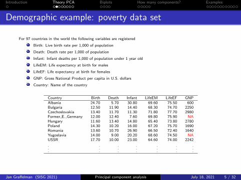
Demographic example: poverty data set

For 97 countries in the world the following variables are registered

Birth: Live birth rate per 1,000 of population

Death: Death rate per 1,000 of population

Infant: Infant deaths per 1,000 of population under 1 year old

LifeEM: Life expectancy at birth for males

LifeEF: Life expectancy at birth for females

GNP: Gross National Product per capita in U.S. dollars

Country: Name of the country

Country Birth Death Infant LifeEM LifeEF GNPAlbania 24.70 5.70 30.80 69.60 75.50 600Bulgaria 12.50 11.90 14.40 68.30 74.70 2250Czechoslovakia 13.40 11.70 11.30 71.80 77.70 2980Former E. Germany 12.00 12.40 7.60 69.80 75.90 NAHungary 11.60 13.40 14.80 65.40 73.80 2780Poland 14.30 10.20 16.00 67.20 75.70 1690Romania 13.60 10.70 26.90 66.50 72.40 1640Yugoslavia 14.00 9.00 20.20 68.60 74.50 NAUSSR 17.70 10.00 23.00 64.60 74.00 2242

.

.

.

.

.

.

.

.

.

.

.

.

.

.

.

.

.

.

.

.

.



Demographic example: poverty data set

Birth Death Infant LifeEM LifeEF GNP

Alb 24.70 5.70 30.80 69.60 75.50 600Bul 12.50 11.90 14.40 68.30 74.70 2250Cze 13.40 11.70 11.30 71.80 77.70 2980E.G 12.00 12.40 7.60 69.80 75.90 NAHun 11.60 13.40 14.80 65.40 73.80 2780Pol 14.30 10.20 16.00 67.20 75.70 1690Rom 13.60 10.70 26.90 66.50 72.40 1640Yug 14.00 9.00 20.20 68.60 74.50 NAUSSR 17.70 10.00 23.00 64.60 74.00 2242

.

.

.

.

.

.

.

.

.

.

.

.

.

.

.

.

.

.

.

.

.

R−Fp

●

●●

●

●●

●●

●

●

●

●

●

● ●●

●

●

●

●

●

●●

●

●

●

●

●

●

●

●

●

●

●

●

●

●●

●

●

●

●

●

●

●

●●

●●

●

●

●

●

●

●●

●

●

●

●●

●

●

●

●

●

●

●

●

●

●

●

●

●

●

●

●

●

●

●

●

●

●

●

●

●

●

●

●

●

●

●

●

●

●

●

●

●

●

●

●

●

●

Bol

Mex

Afg

Ban

Ang

Con

Eth

Gab

Gam

Mal

Moz

Nig

Sie

Som

SudCam

Guy

Per

Ira

IraSau

Tur IndInd

Mon

Nep

Pak

Alg

Bot

Egy

Gha

Ken

Lib MorNam

Sou

Swa

Uga

Tan

ZaiZam

Zim

BulCze

Hun

PolRom

USSBye

Ukr

Uru

BelFin

Den

Fra

Ger

GreIre

Ita

Net

Nor

PorSpa

Swe

Swi

U.K

AusJap Can

U.S

For

Yug

Kor

Alb

Arg

Bra

ChiCol Ecu

ParVenBah

Isr

JorKuw

OmaUni

Chi

Hon

MalPhi

Sin

Sri

Tha

Tun

LebVie

Death

Birth

Infant

LifeEF

lnGNP

LifeEM



Genetic example: (10 SNPs of the CHD sample of the 1,000G project)

ID SNP1 SNP2 SNP3 SNP4 SNP5 SNP6 SNP7 SNP8 SNP9 SNP10

NA17962 2 0 0 2 2 0 0 1 0 2

NA17965 1 0 1 2 1 2 2 0 0 1

NA17966 1 1 1 1 0 1 1 2 0 2

NA17967 0 2 1 1 2 1 0 0 0 1

NA17968 1 0 1 1 1 2 1 2 1 2

NA17969 2 2 0 1 1 2 1 1 1 2

NA17970 1 1 2 0 2 0 2 0 0 1

NA17972 1 2 2 2 2 0 1 0 2 0

NA17974 0 2 2 0 2 1 2 1 1 1

NA17975 2 0 0 0 2 1 2 2 2 0

NA17976 0 2 2 1 1 0 0 1 2 0

NA17977 1 0 1 2 1 2 2 1 1 1

NA17978 2 1 1 1 1 1 1 2 2 1

NA17979 1 0 2 1 0 2 0 0 1 0

NA17980 0 0 0 2 0 0 0 2 1 0

NA17981 1 0 0 0 1 2 2 1 1 1

NA17982 1 1 2 1 2 2 0 1 1 0

NA17983 1 0 1 0 2 0 0 2 1 0

NA17986 1 0 0 0 1 2 2 1 1 1

NA17987 0 1 2 0 2 1 2 0 0 1

NA17988 2 1 0 1 0 1 0 0 2 2

NA17989 1 1 1 1 2 1 2 1 1 1

NA17990 1 2 2 1 1 1 2 0 1 1

NA17993 0 2 1 1 1 2 2 0 0 0

NA17995 0 1 1 1 0 1 0 1 1 0

NA17996 1 1 1 1 1 0 1 1 1 1

NA17997 0 1 1 2 1 2 2 2 0 1

NA17998 1 0 0 2 2 1 1 2 0 1

NA17999 2 2 1 0 1 1 0 1 1 1

NA18101 1 1 2 0 1 2 0 2 0 1

.

.

.

.

.

.

.

.

.

.

.

.

.

.

.

.

.

.

.

.

.

.

.

.

.

.

.

.

.

.

.

.

.

rs1110052_T

rs9442373_Crs3813204_A

rs2274264_G

rs9439458_C

rs4074196_C

rs12044597_G

rs6661597_T

rs4648807_T

rs12045693_C



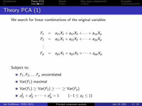
Theory PCA (1)

We search for linear combinations of the original variables

F1 = a11X1 + a12X2 + · · · + a1pXp

F2 = a21X1 + a22X2 + · · · + a2pXp

...

Fp = ap1X1 + ap2X2 + · · · + appXp

Subject to:

F1,F2, . . .Fp uncorrelated

Var(F1) maximal

Var(F1) ≥ Var(F2) ≥ · · · ≥ Var(Fp)

a2i1 + a2

i2 + · · · + a2ip = 1 (−1 ≤ aij ≤ 1)



Theory PCA

With some algebra, it can be shown that

The coefficients of the linear combinations are the eigenvectors of thecovariance matrix.

The eigenvalues of the covariance matrix are the variances of the principalcomponents.

All coefficients and eigenvalues can efficiently be obtained by the spectraldecomposition of the covariance matrix:

Σ = ADλA′.

We will use the sample covariance matrix S to estimate Σ

S = ADλA′.

and estimate the components by sample components:

F = Xc A(n × p) (n × p) (p × p)



Geometric Interpretation (p = 2)

●

●

●

●●

●

●

●

●

●

●

●

●

●

●

●

●

●

●

●●

●

●

●

●

●

●●

●

●

●

●

●

●

●

●

●

●

●

●

●●

●

●

●

●

●

●

●

●

●

●

●

●

●

●

●

●

●

●

●

●

●

●

●

●

●● ●

●

●

●

●

●

●

●

●

●

●

●

●

●

● ●

●

●

●

●

●

●

●

●

●

●

●

●

●

●

●

●

X1

X2

Z 1

Z2



Computing the PCA solution by the SVD

Xc = UDsA′

Fp = XcA = UDsA′A = UDs

1

n − 1Fp′Fp =

1

n − 1(UDs )′UDs =

1

n − 1D2s = Dλ λi =

d2i

n − 1

Fs = FpD− 1

2λ

=√n − 1UDsD−1

s =√n − 1U

1

n − 1Fs′Fs = U′U = I.

and we obtain factorizations for making biplots

Xc = FpA′ or Xc = Fs (1

√n − 1

ADs )′

Notes:

The SVD paves the way for biplot construction

The variables are also LC of the components

PCA provides a low rank approximation to the centred data matrix that is optimal in the least squares sense

PCA also provides a low rank approximation to the covariance matrix that is optimal in the least squaressense



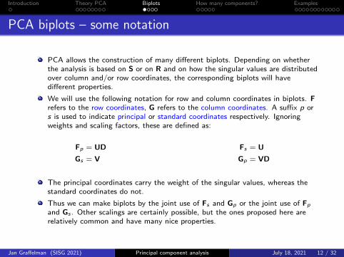
PCA biplots – some notation

PCA allows the construction of many different biplots. Depending on whetherthe analysis is based on S or on R and on how the singular values are distributedover column and/or row coordinates, the corresponding biplots will havedifferent properties.

We will use the following notation for row and column coordinates in biplots. Frefers to the row coordinates, G refers to the column coordinates. A suffix p ors is used to indicate principal or standard coordinates respectively. Ignoringweights and scaling factors, these are defined as:

Fp = UD

Gs = V

Fs = U

Gp = VD

The principal coordinates carry the weight of the singular values, whereas thestandard coordinates do not.

Thus we can make biplots by the joint use of Fs and Gp or the joint use of Fp

and Gs . Other scalings are certainly possible, but the ones proposed here arerelatively common and have many nice properties.



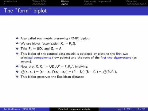
The ”form” biplot

Also called row metric preserving (RMP) biplot.

We use biplot factorization Xc = FpGs′

Take Fp = UDs and Gs = A

This biplot of the centred data matrix is obtained by plotting the first twoprincipal components (row points) and the rows of the first two eigenvectors (asarrows).

Note that XcXc′ = UDλU′ = FpFp

′, implying:

d2E (xi , xi′ ) = (xi − xi′ )

′(xi − xi′ ) = (fi − fi′ )′(fi − fi′ ) = d2

E (fi , fi′ ).

This biplot preserves the Euclidean distance



The ”covariance” biplot

Also called column-metric preserving (CMP) biplot.

We use biplot factorization Xc = FsGp′

Take Fs =√n − 1U and Gp = 1√

n−1ADs .

Gp : contains the covariances between variables and components.

1

(n − 1)Xc′Fs =

1

(n − 1)ADsU′U

√n − 1 =

1√n − 1

ADs = Gp

This biplot of the centred data matrix is obtained by plotting the first twostandardized principal components (row points) and the covariances of the firsttwo components with the variables (as arrows).

XcS−1Xc′ = (n − 1)UU′ = FsFs

′

d2M(xi , xi′ ) = (xi − xi′ )

′S−1(xi − xi′ ) = (fi − fi′ )′(fi − fi′ ) = d2

E (fi , fi′ ).

Euclidean distances in the biplot represent Mahalanobis distances.



More properties of the covariance biplot

GpGp′ = ADλA′ = S = 1

n−1Xc′Xc

cos(gi , gj ) =gi′gj

‖gi‖‖gj‖=

1n−1

xi′xj

1√n−1‖xi‖ 1√

n−1‖xj‖

=1

n−1xi′xj√

1n−1

xi ′xi√

1n−1

xj ′xj= r(xi , xj )

‖gi ‖=√

(1/(n − 1))xi ′xi = sxi

For standardized data, ‖gi ‖=√

r2(xi ,F1) + r2(xi ,F2) + · · ·+ r2(xi ,Fp) =√R2

Note that these are all full space results.



How many components ?

Criteria:

Percentage of explained variance (> 80%).

Size of the eigenvalue (> λ).

The scree plot.

Significance tests with the eigenvalues.



How many components ?

We have:

tr(S) = tr(ADλA′) = tr(Dλ).

p∑i=1

V (Xi ) =

p∑i=1

V (Fi ) =

p∑i=1

λi .

Component F1 F2 · · · FpVariance λ1 λ2 · · · λpFraction λ1/

∑λi λ2/

∑λi · · · λp/

∑λi

Cum. Fraction λ1/∑λi (λ1 + λ2)/

∑λi · · ·

∑λi/

∑λi



The scree plot (poverty data set; correlation-based)

1 2 3 4 5 6

01

23

45

Scree−plot

PC

Eig

enva

lue



Types of PCA

There are two types of PCA. Computations can be based on

the covariance matrix (S)

Not invariant w.r.t. the scale of measurementThe variable with the largest variance dominatesSome authors focus on components with λi > λ

the correlation matrix (R)

Invariant w.r.t. the scale of measurementAll variables have equal weightSome authors focus on components with λi > 1



Interpretation

Components can be interpreted with the aid of:

the coefficients

the correlations between variables and components

the biplot

If the aim is to get a picture of the data matrix, then interpretationof the components may not be needed.



Two examples

UN poverty data (n = 97 countries, p = 6 variables)

1,000 Genomes project CHD sample (n = 109, p = 28, 158SNPs)



Scatterplot matrix poverty data

10 30 50

1030

50

Birth5

1525

●

●●●●

●●

●●

●

●

●

●

●

● ●

●●●

●

●

●

●

●●

●

●

●

● ●●●

●

●

●

●

●

●

●●

●●

●

●

●

●

● ●

●

●●●

●

●

●●

●

●

●●

●

●

●

●

● ●

●●

●

●

●

●

●

●

●

●

●

●

●

●

●

●

●

●

●

●

●

●

●

●

●

●

●

●●●

●

Death

050

150

●

●●●● ●

●● ●

●●

●

●

●

●

●

●●

●

●

● ●

●

●●●●●● ●● ●●●

● ●●●●● ● ●

●

●

●

●

●

●

●

●●

●●

●

●

●

●

●

●

●

● ●

●

●

●

●

●

●●

●

●

●

●●

●

●

●

●

●

●

●

●

●

●●

●

●

●

●

●

●

●

●●

● ●

●

●

●●●

●●

●● ●

● ●

●

●

●

●

●

●●

●

●

●●

●

●● ●● ●●●●● ●●

● ●● ●●●●●

●

●

●

●

●

●

●

●●

●●

●

●

●

●

●

●

●

●●

●

●

●

●

●

●●

●

●

●

●●

●

●

●

●

●

●

●

●

●

●●

●

●

●

●

●

●

●

●●

●●

●

Infant

4060

●●

●

●

●●●

●

●●●

●

●

●

●

● ●

●

●

●

●●

●

●●●●●

●

●●

●

●●

●●●

●●

●

●●

●

●

●

●

●

●

●

●●●

●

●

●

●

●

●

●

●

●●

●

●

●

●

●●

● ●

●

●

●

●

●

●

●

●

●

●

●

●

●

●

●

●

●

●

●

●

●

●

●●

● ●

●

●●

●

●

●●●

●

●● ●

●

●

●

●

● ●

●

●

●

●●

●

●●●● ●

●

●●

●

●●

●●●●

●

●

●●

●

●

●

●

●

●

●

●●●

●

●

●

●

●

●

●

●

●●

●

●

●

●

●●

● ●

●

●

●

●

●

●

●

●

●

●

●

●

●

●

●

●

●

●

●

●

●

●

●●●●

●

●●

●

●

●● ●

●

●●●

●

●

●

●

● ●

●

●

●

●●

●

●●●●●

●

●●●

●●

●●●●●

●

●●

●

●

●

●

●

●

●

●● ●

●

●

●

●

●

●

●

●

●●

●

●

●

●

●●

● ●

●

●

●

●

●

●

●

●

●

●

●

●

●

●

●

●

●

●

●

●

●

●

●●

●●

● LifeEM

4060

80

●●

●●●

●

●● ●

●●

●

●

●

●

●●

●

●●

●●

●

●●

●

●●

●

●●

●

●

●

●●●

●●

●●

●

●

●

●

●

●

●

●

●●●●

●

●

●

●

●

●

●

●●

●

●

●

●

●

●

●●

●

●

●

●

●

●

●

●

●

●●

●

●

●

●

●

●

●

●

●●

●

●●

●●

●

● ●

●●

●●

●● ●●

●●

●

●

●

●●●

●●

●●

●

●●

●

●●

●

●●

●

●

●

●●●●

●

●●

●

●

●

●

●

●

●

●

●●●●

●

●

●

●

●

●

●

●●

●

●

●

●

●

●

●●

●

●

●

●

●

●

●

●

●

●●

●

●

●

●

●

●

●

●

●●

●

●●●

●

●

●●

●●

●●

●●●

●●

●

●

●

●

●●

●

●●

●●

●

●●●

●●

●

●●●

●

●

●●●●●

●●●

●

●

●

●

●

●

●

●● ●●

●

●

●

●

●

●

●

●●

●

●

●

●

●

●

●●

●

●

●

●

●

●

●

●

●

●●

●

●

●

●

●

●

●

●

●●

●

●●

●●

●

●●

●●

●●

●●●

●●

●

●

●

●

●●

●

●●

●●

●

●●

●

●●

●

●●

●

●

●

●●●

●●

●●

●

●

●

●

●

●

●

●

●●●●

●

●

●

●

●

●

●

●●

●

●

●

●

●

●

●●

●

●

●

●

●

●

●

●

●

●●

●

●

●

●

●

●

●

●

●●

●

●●

●●

● LifeEF

10 30 50

015

000

3500

0

●●●●●● ●●●

●●

●● ● ●●

●●● ●●

●

●

●

●

●

●

●

● ●

●

●

●

●

●

●●

●

●●

●

●

●●

●

●

●

●

●

●

●

●●

●

●●●

● ●● ●

●

●● ●

●●

●● ●● ●● ●

●

●●

●● ●● ●

●

● ●●●●● ●●

5 15 25

●●● ●

●●●● ●●

●

●●● ●●

● ●●● ●

●

●

●

●

●

●

●

●●

●

●

●

●

●

●●

●

●●

●

●

●●

●

●

●

●

●

●

●

●●

●

●●●

● ●●●

●

●●●

●●

●● ●● ●●●

●

●●

●● ● ●●

●

●●●●●●●●

0 50 150

●●

●●● ●●●●

●●

●● ● ●●

● ●●● ●

●

●

●

●

●

●

●

●●

●

●

●

●

●

●●

●

●●

●

●

●●

●

●

●

●

●

●

●

●●

●

●●●

● ●●●

●

●● ●

●●

●● ●● ●●●

●

●●

●●● ●●

●

● ●●●●●●●

40 60

●●

●●●●● ●●

●●

●●●●●

●●●●●

●

●

●

●

●

●

●

●●

●

●

●

●

●

●●

●

●●

●

●

● ●

●

●

●

●

●

●

●

● ●

●

● ●●

●● ● ●

●

●●●

●●

● ●● ●● ● ●

●

●●

●●●● ●

●

●● ●●●●● ●

40 60 80

●●

●●●●● ●●

●●

●●●●●

●●●●●

●

●

●

●

●

●

●

●●

●

●

●

●

●

●●

●

●●

●

●

● ●

●

●

●

●

●

●

●

● ●

●

● ●●

●● ● ●

●

●●●

●●

● ●● ●● ● ●

●

●●

●●●● ●

●

●● ●● ●●● ●

0 15000 35000

015

000

3500

0

GNP



Correlation matrix and variance decomposition

Birth Death Infant LifeEM LifeEF lnGNPBirth 1.00 0.49 0.86 -0.87 -0.89 -0.74

Death 0.49 1.00 0.65 -0.73 -0.69 -0.51Infant 0.86 0.65 1.00 -0.94 -0.96 -0.79

LifeEM -0.87 -0.73 -0.94 1.00 0.98 0.81LifeEF -0.89 -0.69 -0.96 0.98 1.00 0.83lnGNP -0.74 -0.51 -0.79 0.81 0.83 1.00

PC1 PC2 PC3 PC4 PC5 PC6λ 4.96 0.58 0.28 0.11 0.06 0.01fraction 0.83 0.10 0.05 0.02 0.01 0.00cumulative 0.83 0.92 0.97 0.99 1.00 1.00



Coefficients (eigenvectors) and correlations

Coefficients

PC1 PC2 PC3 PC4 PC5 PC6

Birth 0.40 -0.37 0.46 -0.65 0.23 -0.07Death 0.33 0.88 -0.06 -0.28 0.20 0.02Infant 0.43 -0.07 0.17 0.65 0.58 -0.14

LifeEM -0.44 -0.05 -0.09 -0.14 0.66 0.59LifeEF -0.44 0.05 -0.11 -0.17 0.36 -0.79lnGNP -0.39 0.28 0.85 0.16 -0.11 0.03

Correlations

PC1 PC2 PC3 PC4 PC5 PC6

Birth 0.90 -0.28 0.25 -0.22 0.05 -0.01Death 0.74 0.67 -0.03 -0.09 0.05 0.00Infant 0.96 -0.05 0.09 0.22 0.14 -0.02

LifeEM -0.98 -0.03 -0.05 -0.05 0.15 0.07LifeEF -0.99 0.03 -0.06 -0.06 0.09 -0.09lnGNP -0.86 0.22 0.45 0.06 -0.03 0.00



Form biplot (principal components)

Bol

Mex

Afg

Ban

Ang

Con

Eth

Gab

Gam

Mal

Moz

Nig

Sie

Som

SudCam

Guy

Per

Ira

IraSau

Tur IndInd

Mon

Nep

Pak

Alg

Bot

Egy

Gha

KenLibMor

NamSou

Swa

Uga

Tan

ZaiZam

Zim

BulCze

Hun

PolRomUSSBye

Ukr

Uru

BelFin

Den

Fra

Ger

GreIre

ItaNet

Nor

PorSpa

SweSwi

U.K

AusJap CanU.S

For

Yug

Kor

Alb

Arg

Bra

ChiCol Ecu

ParVenBah

Isr

JorKuw

OmaUni

Chi

Hon

MalPhi

Sin

Sri

Tha

Tun

LebVie

Death

Birth

Infant

LifeEF

lnGNP

LifeEM



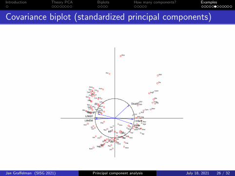
Covariance biplot (standardized principal components)

Bol

Mex

Afg

Ban

Ang

Con

Eth

Gab

Gam

Mal

Moz

Nig

Sie

Som

Sud

Cam

Guy

Per

Ira

Ira

Sau

Tur IndInd

Mon

Nep

Pak

Alg

Bot

Egy

Gha

Ken

LibMor

Nam

Sou

Swa

Uga

Tan

Zai

Zam

Zim

BulCze

Hun

PolRom

USSBye

Ukr

Uru

BelFin

Den

Fra

Ger

GreIre

Ita

Net

Nor

Por

Spa

Swe

Swi

U.K

AusJap

Can

U.S

For

Yug

Kor

Alb

Arg

Bra

Chi

Col Ecu

ParVenBah

Isr

JorKuw

Oma

Uni

Chi

Hon

Mal

Phi

Sin

Sri

Tha

Tun

Leb

Vie

Death

Birth

Infant

LifeEFlnGNP

LifeEM



Four PCA biplots

S−Form

BraGuy

Per

Afg

IraTur BanIndInd

NepPak

AngEthGab GamMor

MozNam SieSou

CamVie

BolEcu

IraSauMon

Alg

BotCon

GhaKen

LibMal

NigSomSud Swa

UgaTan

ZaiZam

Zim

BulCzeHunPolRom

USSByeUkrArgUruBelFinDenFraGerGre

IreIta

NetNorPorSpa

SweSwiU.KAusJap

CanU.S ChiHonFor Yug

AlbChi Col

ParVenMex

BahIsr

JorKuw

Oma

Uni

MalPhi

Sin Sri Tha

Egy

TunLebKor

Death

Infant

Birth

LifeEMLifeEF

lnGNP

S−Covariance

Bra

Guy

Per

Afg

Ira

TurBanIndInd

Nep

Pak

AngEthGab

Gam

Mor

Moz

Nam

Sie

Sou

Cam

Vie

BolEcu

IraSau

Mon

Alg

Bot

Con

Gha

Ken

Lib

Mal

Nig

SomSudSwa

Uga

Tan

Zai

Zam

Zim

BulCzeHun

Pol

Rom

USSBye

Ukr

Arg

Uru

BelFin

DenFra

GerGre

Ire

Ita

Net

Nor

Por

Spa

Swe

SwiU.KAus

Jap

Can

U.SChi

HonForYug

Alb

ChiCol

Par

Ven

Mex

Bah

Isr

Jor

Kuw

Oma

Uni

Mal

Phi

Sin SriTha

Egy

Tun

Leb

Kor

Death Infant

Birth

LifeEMLifeEFlnGNP

R−Form

Bol

Mex

Afg

Ban

Ang

Con

EthGab

Gam

Mal

Moz

Nig

Sie

Som

Sud Cam

GuyPer

Ira

IraSauTur IndInd

Mon

Nep

PakAlg

Bot

Egy

Gha

KenLibMor

NamSou

SwaUga

Tan

ZaiZam

Zim

BulCze

Hun

PolRomUSSBye

Ukr

Uru

BelFin

Den

Fra

Ger

GreIreIta

Net

Nor

PorSpa

SweSwi

U.K

AusJap CanU.S

For

Yug

Kor

Alb

Arg

BraChi

Col EcuParVenBah

Isr

JorKuw

OmaUni

Chi

Hon

MalPhi

Sin

Sri

Tha

Tun

LebVie

Death

Birth

Infant

LifeEF

lnGNP

LifeEM

R−Covariance

Bol

Mex

Afg

Ban

Ang

Con

Eth

Gab

Gam

Mal

Moz

Nig

Sie

Som

SudCam

Guy

Per

Ira

IraSau

Tur IndInd

Mon

Nep

Pak

Alg

Bot

Egy

Gha

Ken

LibMorNam

Sou

Swa

Uga

Tan

ZaiZam

Zim

BulCze

Hun

PolRom

USSBye

Ukr

Uru

BelFin

Den

Fra

Ger

GreIre

Ita

Net

Nor

Por

Spa

Swe

Swi

U.K

AusJapCan

U.S

For

Yug

Kor

Alb

Arg

Bra

Chi

Col Ecu

ParVenBah

Isr

JorKuw

OmaUni

Chi

Hon

MalPhi

Sin

Sri

Tha

Tun

Leb

Vie

Death

BirthInfant

LifeEFlnGNP

LifeEM



Genetic example: CHD (Chinese in Metropolitan Denver) data; 1,000G project

Genetic data typically filtered prior to PCA, using multiple criteria:

chromosome (X chromosome mostly excluded)

missingness

MAF

test results for HWE

correlation structure (LD pruning)

...

Here we use 24.087 autosomal, complete, highly polymorphic SNPs of109 CHD individuals.



CHD (Chinese in Metropolitan Denver) data; 1,000G project

−50 0 50

−10

0−

80−

60−

40−

200

20

Scatterplot PC1 − PC2

First principal axis (1.41%)

Sec

ond

prin

cipa

l axi

s (1

.4%

)

NA17981

NA17986 NA17976

NA18116

0 20 40 60 80 100

050

100

150

200

Scree plot

PC

Eig

enva

lue



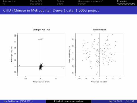
Observations

The joint plot of individuals and variables is too dense.

p > n and there are only n − 1 PCs with non-zero variance.

Explained variance is very low (typical for large-scale geneticapplications).

PCA detects outliers.

In this application, outliers are documented related pairs (one FS;one PO; one 2ND).

A covariance based PCA is the natural choice.

The form biplot is the natural choice for this data.

Computationally not attractive to extract eigenvectors of S.



CHD (Chinese in Metropolitan Denver) data; 1,000G project

−50 0 50

−20

020

4060

8010

0

Scatterplot PC1 − PC3


Thi

rd p

rinci

pal a

xis

(1.2

%)

NA17980

NA18150

−30 −20 −10 0 10 20 30

−30

−20

−10

010

20

Outliers removed


Sec

ond

prin

cipa

l axi

s (1

.1%

)



References

Anderson, T.W. (1984) An Introduction to Multivariate Statistical Analysis, Second edition, John Wiley,New York. Chapter 11.

Johnson & Wichern, (2002) Applied Multivariate Statistical Analysis, 5th edition, Prentice Hall, Chapter 8.

Jolliffe, I.T. (1986) Principal Component Analysis, Springer-Verlag, New York.

Manly, B.F.J. (1989) Multivariate statistical methods: a primer. 3rd edition. Chapman and Hall, London.Chapter 6.

Mardia, K.V. et al. (1979) Multivariate Analysis. Academic press. Chapter 10.


Jan Gra elman - si.biostat.washington.edu

Documents

Transcript of Jan Gra elman - si.biostat.washington.edu