Welcome to the

JakeOmatic

Data analysis software for fishery managers

Version 2.4

July 2006

Please address all questions or comments to:

Kevin Rogers Colorado Division of Wildlife

PO Box 775777 Steamboat Springs, CO 80477

(970) 846-7145 kevin.rogers@state.co.us

2

TABLE OF CONTENTS: Purpose 3 Quickstart 3 Installation 3 Startup 4 Data Entry 5 Printing/Export Options 9 Lake Module 10 Input 10 Output 10 Stream Module – Two Pass Removal 11 Input 11 Output 12 Stream Module – Mark Recapture 14 Input 14 Output 14 Species Codes 14 Estimate Weight 15 High Lake Plants 16 Hooking Mortality 17 Grascarp 18 About… 19 Granby Lake Trout Database 19 Advanced Topics 20 Troubleshooting 22 Known Bugs 22 Literature Cited 22 Appendices 24 Species Code List 25 List of New Features 28 Formulae Used in Version 2.2 30

3

PURPOSE Fish data analysis tool that can store and interpret stream and lake data in a file

format that can be read by ADAMAS – Colorado’s statewide fish database

QUICKSTART (for those familiar with Version 1) Install software off CD, website, or CDOW network drive

Open the installer folder and find six files Click on the setup.exe icon Follow installer instructions

• I would not change the default installation location (destination folder) – let the installer cam put the application in your “Program Files” folder

• This will allow you to access the program from your start menu The formats of the first three modules are basically the same as Version 1.9, with

some key changes (for a detailed list of new features, see List of New Features The program is running the minute you open it – select the module you want

to use and hit GO Click the DONE button anytime you want to close a module. The default windows X close button in the upper right corner grayed out – it

did many bad things

INSTALLATION Installing off CD

Open the installer folder, and double click on the “Setup.exe” icon • Follow directions for installation

Installing off Colorado Division of Wildlife website Go to http://wildlife.state.co.us/Research/Aquatic/Software Click on the JakeOmatic 2.4 link This is a zipped file, so unzip and follow directions above

Installing off CDOW server (for CDOW employees only) Since the JakeOmatic and various support documents are large (20Mb), I have

put them on the Denver server rather than emailing them to you. They are on the same drive as Terry’s Trans5 stuff, so you should already have the server mapped on your computer. If you would prefer I email the files to you, let me know…

Click on the “My Computer” icon on your desktop Find the dowhq012K\aqhatch server icon

• If the dowhq012K\aqhatch server is not mapped to your computer… ♦ Right click on you’re “My Computer” icon ♦ Click on “Map Network Drive” ♦ Enter \\ dowhq012K\aqhatch in the lower box ♦ Click OK

4

• Click open the “JakeOmatic 2.4” folder Open the installer folder, and double click on the “Setup.exe” icon

Follow the directions for installation This will install the JakeOmatic with a “Support” folder containing support

documents in your “Program Files” on your hard drive • DO NOT move or rename the “Support” folder as it contains files vital to

the operation of the program • The “Support” folder contains…

♦ This manual (MANUAL 2.4b.doc) ♦ An Excel spreadsheet (WatercodesV2.xls) that contains water codes

for water bodies in the state sorted by lakes and streams This is a large file – to make it more manageable, you can sort by

biologist, then highlight just your waters, and copy/paste them into a new spreadsheet

Alternatively, you can just use the “Find” feature in Excel to find the specific body of water you want a water code for

♦ Stream and lake Excel templates (LakeTemplateTAB.xls and StreamTemplateTAB.xls)

Allows you to enter data in Excel if you want to, rather than into the JakeOmatic directly

See directions in the data entry section for use ♦ Sample stream and lake field data entry sheets ♦ Three sample data sets to help get familiar with the capabilities of the

JakeOmatic (one for each module – LakeTest.txt; StreamTest.txt, and RecapTest.txt)

For best results, set your monitor resolution to at least 1024x768 pixels rather than say 800x600 pixels. To change or check your resolution

• Click the start menu settings control panels • Double click on the “display” icon and move the slider to change

resolution To open the application, Click on the start menu Programs JakeOmatic2.4 Alternatively, you can set up a shortcut to the JakeOmatic on your desktop by...

Finding the program file (JakeOmatic2.4) in the “JakeOmatic” folder in the “Program Files” folder on your hard drive (C:\Program Files\JakeOmatic2.4

Right-click on it and select “Create Shortcut” Drag that shortcut to your desktop

5

FIRE UP THE JakeOmatic Unlike Version 1.9, Version 2 is already running when you open the program. Toggle through the different panels using the little arrow button next to the upper

left corner of the convicts Alternatively, you can left click on the big picture to select the module you want

to use The micro-pictures in this popup look great on my Mac but lousy on your PC.

That is because PC graphic capabilities are worthless. You were the one that chose to work with an inferior operating system – deal with it!

Click the GO button on the right side of the window to start the module you have selected

Click the DONE button to stop any panel The default Windows close box (X in the upper right corner) is now gone as

clicking it did bad things

DATA ENTRY (common to all modules) Station specific information

Fill in information in the box in the upper left See each module’s instructions below for specific information As before, you can write as much as you want in the NOTES field and use any

punctuation – you just can’t hit return. Think of the notes as being contained in a cell on a spreadsheet – if you hit return it moves you to a different cell, messing up the formatting for everything else. If your comments are too verbose to fit in the NOTES pane on the LEVEL II form, print a PANEL as well – the field is even larger there.

Entering raw data into the spreadsheet table This field operates just like a spreadsheet, though the arrow keys do not work.

Use the mouse to move anywhere in the table. Tab to move right and shift-tab to move left. Return moves you down to the next row • Many of us enjoy using the arrow keys to navigate around a spreadsheet,

but the table function I am using for this program does not support the arrow keys. In practice it is actually faster to use the shift-tab combination to back up since you can do that with your left hand and enter numbers with your right. It takes a little getting used to, but is worth the time spent getting comfortable with it.

6

• DO NOT – tab four times to get to the next row – use the return key to drop down a row otherwise will overwrite data as screen fills

• DO NOT – leave the status column blank, or not all metrics will be calculated (such as mean weight)

Most fields will be automatically carried down from the row above to speed data entry • Double click on the cell if the numbers or letters need to be changed

Columns • Species

♦ You must use the 3 letter species code here (all caps) ♦ If you are unsure of the species code, click on the LUT (species lookup

table) button and enter in the species name (all caps) ♦ Don’t tell Harry, but if you need to code a fish differently (say to get a

population estimate on a batch of adipose clipped rainbows), you can cheat the system by using QQQ or VVV – just make sure to add that comment to the “Notes” field; Names for these codes are “Miscellaneous 1” and “Miscellaneous 2” respectively, and can be found at the bottom of the “Minnows” tab

• Count ♦ This defaults to 1 if you have lengths and weights on individual fish ♦ If you prefer to count fish in length bins, just enter the number of fish

in each length increment here • Length

♦ These can be entered in mm or cm (mm is default) ♦ If you want to enter data in cm, switch the mm/cm toggle

Keep in mind that although you entered this data in cm, the file is stored in mm (to facilitate smooth incorporation to ADAMAS), so if you retrieve the file for later study, the toggle will need to be set to mm

• Weight ♦ These must be entered in grams ♦ If you did not weigh fish, you can estimate their weights for a given

length by clicking the ESTIMATE WEIGHT button This button uses coefficients from the standard relative weight

equations developed for many game fish (shown in the lookup table)

The default relative weight is 93% - or what the average condition of an average fish would be. If your fish appear extra plump or skinny, you can change the relative weight value to be used

♦ Bulk weights – if you have so many fish that it is not practical to weigh and measure each individual, enter an average length and weight, and then the appropriate count. Make sure to include a note in the comments field that explains what was done.

• Status ♦ This field describes which sampling event the fish were captured in

7

♦ Lake surveys Use an E for fish caught by electrofishing, G for gill net, and T for

traps (all caps) Use a number following the letter to designate of catch by

individual stations, nets or traps (e.g. E1, E2, E3… or G1, G2, G3… or T1, T2, T3…

♦ Stream surveys – 2 pass removal Use a 1 or a 2 to represent the pass number in which the fish was

caught ♦ Stream surveys – mark recapture

Use an M for fish captured in the first pass and marked Use a C for fish captured on the second pass that were not marked Use an R for fish captured on the second pass that were marked

(recaptured) • Mark

♦ This field is for batch marks (fin clips, brands, etc) ♦ The JakeOmatic ignores this column, but entry here is useful if you are

porting the data to other programs • TagID

♦ Scroll right to reach this field ♦ This field is for individual fish marks (VI tags, Floy tags, etc) ♦ The JakeOmatic ignores this column, but entry here is useful if you are

porting the data to other programs Entering data into other spreadsheet programs (Excel, Quattro, etc)

There is nothing magical about the format of the entered data files – they are simple tab delimited ASCII text files that can be created in just about any application

If you are partial to using the arrow keys, or want someone else to enter your data on a machine that does not have the JakeOmatic, use the included Excel templates to enter data (StreamTemplateTAB.xls and LakeTemplateTAB.xls) • Open the template in Excel • “Save as” and rename the template before you start saving data to it with a

descriptive name (e.g. 2001WindyGapR.txt) • Replace red text with your site specific information (do not change any of

the black text, or the JakeOmatic will not recognize key information) ♦ New in Version 2: the header information can now be entered in the

second column. If you prefer that approach, use the new TAB templates. Version 1 files formats still work fine as well

• Enter lengths in mm (if you must use cm, you can use the toggle in the JakeOmatic to convert to mm, then resave the file when you click DONE

• Enter weights in grams if you have them • Use the copy down feature in Excel (click on a cell then drag the bottom

right corner to fill in as many additional cells with identical information) to facilitate rapid data entry

8

• When finished, do a “Save as” and make sure the file is saved as ASCII tab delimited text – these files can then be read by the JakeOmatic and ADAMAS

Make sure that all your species codes are supported by the JakeOmatic before you open it in the program, or you will be told that it is not – for every entry!

In practice, it is easier and safer to just get comfortable using the shift-tab keys, and enter the data directly in to the JakeOmatic • The only time you need to use these templates is if you are entering the

data directly into a PDA in the field Retrieving data from your hard drive

Click on the yellow folder icon in the center of the panel while the program is running

Removing rows of bad data If you have entered an entire row of bad data, click the DELETE ROW radio

button A dialog popup window will ask you which row you want to delete

Saving your data If you feel like your computer is going to crash while you are entering a big

data set (you are working on a PC after all), click the SAVE radio button to save the data you are entering to a file. If you are confident and bold, just enter the entire data set and press the DONE button – this will also save data to a file that you specify

Keep in mind that both the SAVE and DONE buttons will write your data to a file in mm only (to facilitate transfer to ADAMAS). This is only a big deal if you quit the JakeOmatic halfway through a data set that you are entering in cm, then come back to enter the remainder at a later date. If this happens, just make sure you enter the remainder in mm.

Remember to use descriptive file names such as 2003BlueRDam.txt for the data files. While you are welcome to use any three letter suffix you like, these are ASCII text files so a .txt is most appropriate.

Submitting data to ADAMAS Just attach the data files to an email to Harry Vermillion at

harry.vermillion@state.co.us with a note telling him you want the data included in ADAMAS

9

PRINTING/EXPORT OPTIONS Keep in mind that if you are running on an older computer/printer, pressing a

print button will tie up your CPU for a bit – be patient or upgrade… Press the LEVEL II button to print or view a Level II form for the survey

If you wish to save the Level II form to a Word file, just click the SAVE button. It will bring up Word with your new document to the front. Save and close that document (and minimize or close Word) to go back to the JakeOmatic running in the background.

To print the Level II form, you have two options • The upper PRINT button prints a nice looking form (no jaggies) on most

Windows2000 platforms – try it first. If the Level II does not print properly, then use the lower PRINT button

• The lower PRINT button takes a screen shot of the panel and prints that. This option prints consistently across machines/printers, but doesn’t look as good because the text has the “jaggies”. If your reports look good using the upper button, consider yourself lucky and stick with it!

• These should both automatically print in landscape format WARNING – the Level II PRINT and SAVE options only work on machines

with Windows2000 or later and Microsoft Word installed. Press the PRINT PANEL button to print a black and white version of the panel

you are looking at Good news - this panel is not a screen dump, and therefore does not have the

jaggies Bad news - it may not print well on some machines. It seems to work great on

CDOW computers running Windows2000. Let me know if that is not the case with your computer, and I will code an alternative…

The EXPORT LF button will export the length frequency histogram data to a file for import into a conventional spreadsheet program for more flexible graphing. This output file now has a header row and cleaner x-axis values

The EXPORT Wr button will export the relative weight scatter plot to a file for import into a conventional spreadsheet program for more flexible graphing (new in Version 2)

10

LAKE MODULE INPUT

Station specific information • Water – name of the lake • Effort – gill nets, traps, electrofishing (e.g. 6x150’ exp gill nets) • Drainage – major drainage (e.g. Yampa River) • Crew – at least include the biologist responsible • Notes – include all other information here (e.g. net locations) • Date – in the following format: mm/dd/yyyy • Water code – from Trans5 or the WatercodesV2.xls spreadsheet in the

“Support” folder • UTM zone • UTM x – this is the 6 digit Easting • UTM y – this is the 7 digit Northing • E hours – enter the total number of hours shocked (e.g. 1.3 hours) • G hours – enter the total number of hours gill nets were fishing (e.g. 6 nets

x12 hours = 72 hours) • T hours – enter the total number of hours your traps were fishing (e.g. 5

traps x14 hours = 70 hours) OUTPUT

Use the species tabs and drop down menu to select a species to analyze Length frequency histogram and a relative weight plot should be updating

automatically while you are entering data • The scale for both these plots can be toggled between mm, cm, and inches

(down arrow at bottom of length-frequency plot) • If nothing shows up on the relative weight plot, it is likely because a

relative weight equation has not yet been developed for the species (you can check in the lookup table (LUT button) to see if a slope and intercept are given) ♦ The red line on the relative weight plot is fixed at 93% for reference.

Wr equations are developed so that a 100% value represents condition in the 75th percentile of populations over the range of the species. If you are more interested in comparing your fish to a range-wide average (say a 50th percentile), then using approximately 93% as a reference is probably more appropriate.

Catch per unit effort (CPUE) • The catch per hour by species is expressed here for 3 gear types

(Electrofishing, Gill nets, and Traps). CPUE for fish greater than stock size (from the lookup table) are given as well

Proportional and relative stock densities (PSD and RSD)

11

• A full blown discussion of these indicies can be found in the AFS book “Fisheries Techniques” (Anderson and Neumann, 1996)

• Keep in mind that many of these species supported by the JakeOmatic do not yet have stock density cutoff sizes established. In those situations, the relative stock density values will be whacky. If you suspect foul play, check the lookup table (LUT button) to see if cutoffs have been developed for a given species.

Mean length and weight (with ranges) • These are expressed in inches and pounds, as these metrics have limited

utility outside of discussions with anglers – and after all “we don’t live in France”

Unlike the stream modules, the lake module will not estimate the weight of fish for you, since you are not able to judge total biomass without a population estimate anyway. In addition, the cutoff sliders (in the length-frequency plot) do not appear in this module, as they are also population estimation features.

STREAM MODULE – 2 PASS REMOVAL INPUT

Station specific information • Water – name of the stream • Location – Station location (e.g. Behind Safeway, Red barn, etc.) • Drainage – major drainage (e.g. Yampa River) • Crew – at least include the biologist responsible • Notes – include all other information here (e.g. survey specific comments,

flows, water chemistry, etc.) • Date – in the following format: mm/dd/yyyy • Water code – from the water code list (WatercodesV2.xls) • UTM zone • UTM x – this is the 6 digit Easting from the downstream terminus of the

station • UTM y – this is the 7 digit Northing from the downstream terminus of the

station • Station length – thalweg distance in feet • Station width – this is the mean width in feet

♦ Jake always recommended calculating a mean by measuring widths at the downstream terminus and at 50 foot intervals as you measure the thalweg ;)

♦ To facilitate calculation of mean width, you can click the X button

12

which invokes…

A – Enter widths (or anything else) to calculate mean from B – Select units of widths entered C – If widths measured in feet, select if numbers after the decimal

represent inches or tenths of a foot D – Read mean width (tenths of a foot follow decimal)

OUTPUT

Use the species tabs and drop down menu to select a species to analyze Length frequency histogram and a relative weight plot should be updating

automatically while you are entering data • The scale for both these plots can be toggled between mm, cm, and inches

(down arrow at bottom of length-frequency plot) • Drag the blue slider cutoff bar to the right or left to establish the minimum

size fish to consider in the population estimate ♦ This defaults to 150 mm since Jake liked to exclude Age 0 trout

because their capture probabilities tend to be very different than those of trout Age 1 and older

Keep in mind that in some high elevation waters, the cutoff may need to be set lower to include all Age 1 fish

Examine the length-frequency plot to decide where the break ought to be

♦ This feature also lets you assess Gold Medal status (12 trout per acre over 14 inches)

Switch the length-frequency units to inches Slide the blue bar over to 14 (or enter 14 directly in the cutoff

window)

13

♦ Unlike Version 1.9, the program now remembers what cutoff you used for each species and will default to it, as well as display it in the LEVEL II

This allows you to have distinct cutoffs for each species analyzed ♦ In Version 2 you will notice that in addition to selecting units for

display, you can also toggle between BEFORE, AFTER, or BETWEEN

BEFORE restricts the analysis to fish to the left of the blue slider AFTER restricts the analysis to fish to the right of the blue slider

(this is the traditional analysis from Version 1.9 and is the default) BETWEEN restricts analysis to fish in between the two slider bars

Though the MAX CUT field will display a value, that value is ignored unless BETWEEN is selected

Tab between English and Metric units in the output window to view population metrics with their associated 95% confidence intervals

1st Pass – number of fish captured in the first pass greater than the minimum size for analysis

2nd Pass - number of fish captured in the first pass greater than the minimum size for analysis

Capture P – this is the capture probability • Keep in mind that if this drops below 0.80, your estimates become less

reliable • If true capture probabilities do vary between passes, and the calculated

capture probability is less than 0.70, not only will your confidence intervals be large, they may not even include the true population values

Population estimate is for the stream reach LEVEL II FORM

While similar to the LAKE LEVEL II in many ways, there are some key differences. The minimum size cutoff is presented (ie the analysis is conducted with data to the right of the blue slider bar). Since the LEVEL II form is a standard reporting format, several output features that are present in the PANEL output are not available in the LEVEL II. For instance, you cannot invoke double slider output it in the LEVEL II. If you want the results of your analyses from data BEFORE or BETWEEN the slider(s), you need to print the PANEL. In addition, the length-frequency table is divided into cm bins, while the cutoff values are always shown in mm (even if you selected the slider position while the units were in cm or inches)

14

STREAM MODULE – MARK RECAPTURE INPUT

Station specific information similar to inputs for the stream module above OUTPUT

Most of the outputs are the same as that for the stream module above Mark – number of fish greater than the minimum size for analysis captured in

the first pass and (M) Capture - number of fish captured in the second pass greater than the

minimum size for analysis (C+R) Recapture – number of marked fish captured in the second pass (R)

MODELS Unlike Version 1.9 which used a maximum likelihood estimator (Otis et al.

1978), Version 2 uses Chapman’s modification of the Petersen method as GOLDMEDL does.

In practice, the results should be virtually identical, though I have noticed that if the assumption of closure is violated then the different approaches may show divergent results

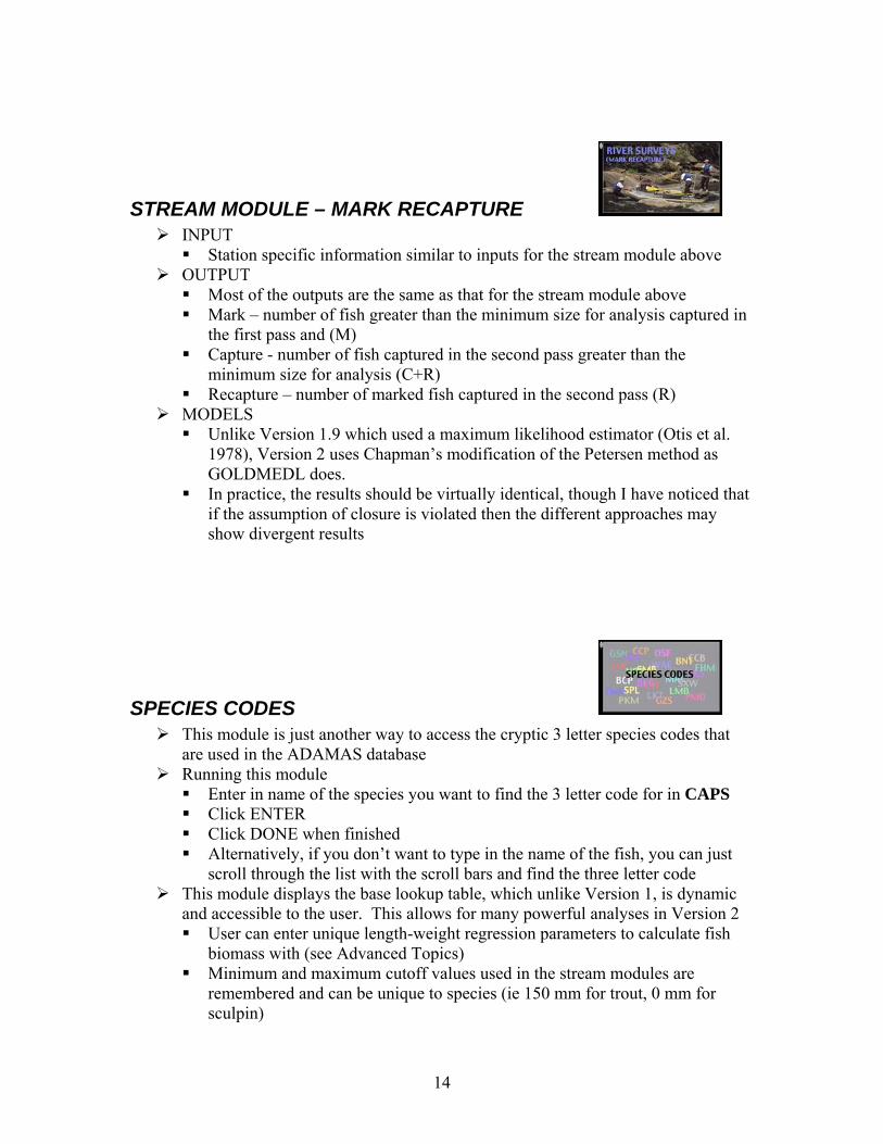
SPECIES CODES This module is just another way to access the cryptic 3 letter species codes that

are used in the ADAMAS database Running this module

Enter in name of the species you want to find the 3 letter code for in CAPS Click ENTER Click DONE when finished Alternatively, if you don’t want to type in the name of the fish, you can just

scroll through the list with the scroll bars and find the three letter code This module displays the base lookup table, which unlike Version 1, is dynamic

and accessible to the user. This allows for many powerful analyses in Version 2 User can enter unique length-weight regression parameters to calculate fish

biomass with (see Advanced Topics) Minimum and maximum cutoff values used in the stream modules are

remembered and can be unique to species (ie 150 mm for trout, 0 mm for sculpin)

15

ESTIMATE WEIGHT This program is an updated version of a program called FishScalz that I wrote in

the early 1990s. It uses the RLP relative weight (Wr) equations developed for most species of game fish to estimate the weight of a fish based on its length and a rough idea of condition (Wr value)

INPUT

A – Select species to analyze – keep in mind that the program will let you select any fish supported by the JakeOmatic . That does not mean that Wr equations exist for the species. Check H and I to see if regression coefficients appear here. If not, then the appropriate equation has not yet been developed at the time of this writing, and the module cannot generate meaningful results.

B – Either enter a relative weight here or… C – Select a rough idea of fish condition with the slider D – Enter the length of the fish in inches and… E – Click ENTER to update the program

OUTPUT F – The estimated weight appears here (in pounds) G – The three letter code used to describe the species in Colorado’s database H – The slope for the RLP Wr equation for the species (0 if not supported) I – The intercept for the RLP Wr equation for the species (0 if not supported) J – Click DONE to end the program and return user to main window

16

HIGH LAKE PLANTS In the 1970s, Wes Nelson of the Division of Wildlife’s Aquatic Research Group

did a considerable amount of work on determining the appropriate stocking densities to use for high mountain lakes in Colorado (Nelson 1987). This module uses his formulae to determine a stocking density to start with. Every high lake is different, and these numbers should only be viewed as a starting recommendation. Condition (relative weight) of fish obtained from standardized samples should be used to fine-tune these numbers for a given lake. This is his pre 1973 formula that appears on the graph in his manual

INPUT A – Lake elevation in feet above sea level B – Lake surface acres C – Fishing pressure (really harvest) Click ENTER to update

OUTPUT D – Recommended stocking density E – Number of fingerling trout to stock Click DONE to close the module and return to the main window

17

HOOKING MORTALITY As part of George Schisler’s graduate work, he developed a model to predict

hooking mortality based on a variety of factors (Schisler and Bergersen 1996). Playing around with this model gives some insight into the relative importance of these factors in trout survival

INPUT

A - Adjust slider to water temperature B - Toggle terminal tackle used C - Toggle active or passive fishing D - Toggle hook location E - Toggle leader status (cut or not) F - Adjust slider to fish length G - Dial in time played H - Dial in time out of water I - Dial in bleeding intensity Click ENTER to update

OUTPUT J – Read probability of dying Click DONE to close the module and return to the main window

18

GRASCARP This model was developed by Swanson and Bergersen (1988) to establish

recommended stocking densities for grass carp. They studied six ponds ranging in elevation from 6100 ft to 8300 ft above sea level – be careful extrapolating outside this range. In practice, numbers recommended by the model are often high. As it is easier to stock more grass carp than to remove ones already stocked, I suggest stocking less than the recommended numbers and evaluating the response. Unfortunately, vegetation control with grass carp often elicits a binomial response – either they wipe out all your vegetation or they don’t do much. It is difficult to fine-tune their numbers to obtain just the right amount of control.

INPUT A – Elevation of lake to receive grass carp B – Length of grass carp to be stocked (in inches) C – Select dominant plant species from this dropdown menu D – Ploidy of grass carp to be stocked E – Dial in plant density F – Percent of vegetation coverage G – Disturbance by boat traffic or other anthropogenic influences that may

curtail feeding H – Desired level of control Click ENTER to update

OUTPUT I – Recommended stocking density Click DONE to close the module and return to the main window

19

ABOUT… LAKE TROUT DATABASE

• Unlike Version 1.9, the path to the actual lake trout database (MacBase5.txt) is hardwired in to the program. Hence this file must remain in the “Support” folder that was installed with your program (C:\Program Files\JakeOmatic2.2\Support).

INPUT • A – Enter the tag number to consider • Click ENTER to update

OUTPUT • B – Species tagged (some northern pike have made it into this database • C – Some lake trout tagged in Blue Mesa Reservoir by Jake clones are in

this database • D – Initial capture history of tagged fish • E – Detailed recapture history • F – Fish length by year (from recapture history) • Click DONE to close the module and return to the main window

OTHER FUN STUFF Just click the buttons… self explanatory

20

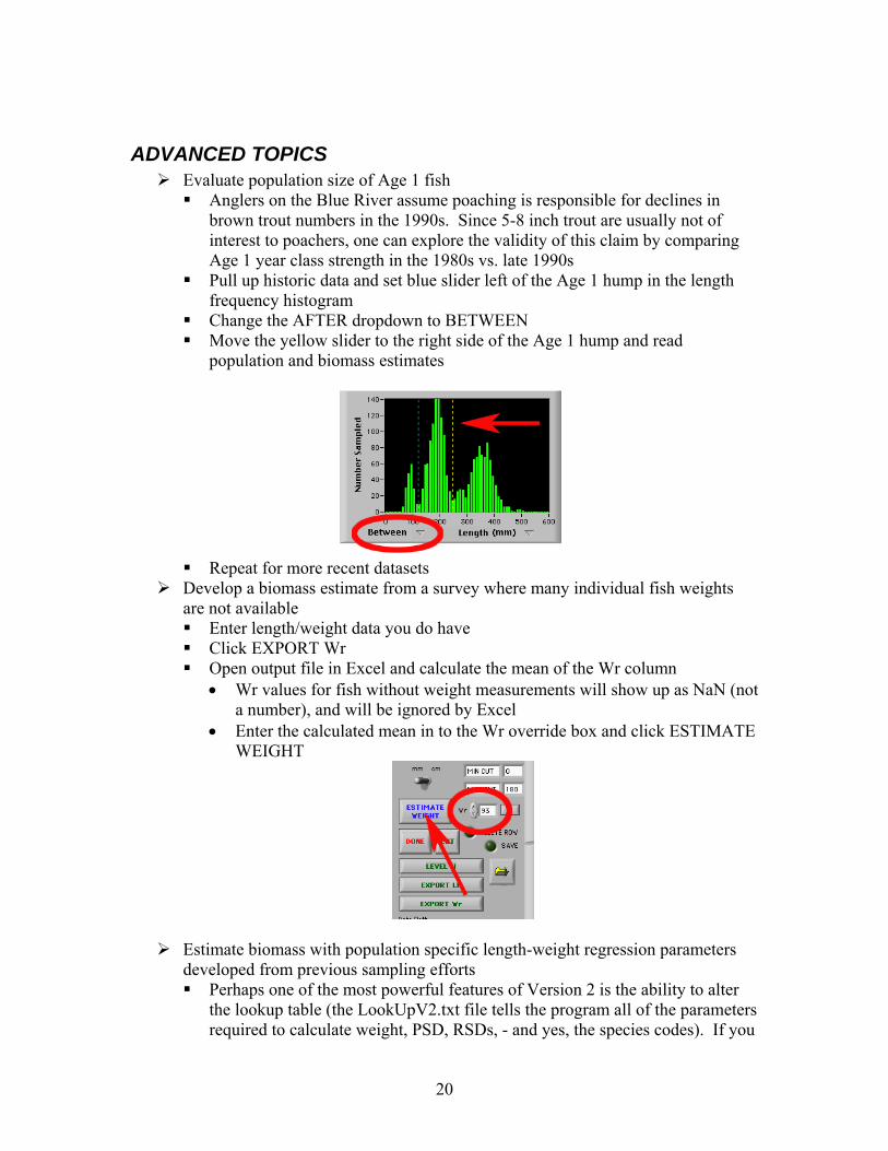
ADVANCED TOPICS Evaluate population size of Age 1 fish

Anglers on the Blue River assume poaching is responsible for declines in brown trout numbers in the 1990s. Since 5-8 inch trout are usually not of interest to poachers, one can explore the validity of this claim by comparing Age 1 year class strength in the 1980s vs. late 1990s

Pull up historic data and set blue slider left of the Age 1 hump in the length frequency histogram

Change the AFTER dropdown to BETWEEN Move the yellow slider to the right side of the Age 1 hump and read

population and biomass estimates

Repeat for more recent datasets

Develop a biomass estimate from a survey where many individual fish weights are not available Enter length/weight data you do have Click EXPORT Wr Open output file in Excel and calculate the mean of the Wr column

• Wr values for fish without weight measurements will show up as NaN (not a number), and will be ignored by Excel

• Enter the calculated mean in to the Wr override box and click ESTIMATE WEIGHT

Estimate biomass with population specific length-weight regression parameters developed from previous sampling efforts Perhaps one of the most powerful features of Version 2 is the ability to alter

the lookup table (the LookUpV2.txt file tells the program all of the parameters required to calculate weight, PSD, RSDs, - and yes, the species codes). If you

21

wish to analyze species not supported on this list, you can add species codes to the lookup table. Keep in mind that they will no longer be compatible with Colorado’s ADAMAS database, and should not be submitted to Harry Vermillion. This flexibility is especially useful if you have specific length-weight relationships developed for a particular population of fish and wish to use those in the estimation of weight for biomass calculations instead of the default Wr values. It is a good idea to save some backup copies of the default lookup table in case you need to put the correct table back. Also critical is that this table remains in the “Support” folder so that the JakeOmatic knows where to find it.

Open the “Support” folder installed with the JakeOmatic (C:\Program Files\JakeOmatic\Support)

Open the file LookUpV2.txt in Word (or any other text editor) Save a copy of this file so you can return to the default parameters Change the slope and intercept (3rd and 4th column) for the species you wish to

analyze to your population specific values and save (file name and location must stay the same for the program to recognize it)

Open dataset in analysis pane and select 100 in the Wr override box Click ESTIMATE WEIGHT button Read new biomass parameters in output

If you prefer to express CPUE in “net nights” as opposed to hours, you can trick the program into calculating it for you by just entering nights in lieu of hours – if you do this, you have to let Harry Vermillion know so that he can fix it when it is entered in to the statewide database (ADAMAS). Make sure that the notes box also includes a comment that clearly states that net nights were used rather than hours.

22

TROUBLESHOOTING Nothing happens when you click GO on the front panel – make sure the

program is running (click the white arrow in the upper left corner if not) Some population metrics not calculated – Check to make sure the status

column populated Only the data visible in the data entry table is written to file – Try hitting

return to move to the next row (do not tab four times to drop down) Population metrics for a stream module analysis using the BETWEEN

function do not match those in the LEVEL II output – this is not an error. The LEVEL II is a standard output format and always shows only the results to the right of the minimum slider cutoff (i.e. the AFTER case)

If the program is locked up and you need to force quit the JakeOmatic, invoke the task manager by pressing ctrl-alt-del and quitting the LabVIEW task.

Two individuals have reported a problem in Version 1.9 that assigned a default file extension of “.vi” to the output files which then prevented the files from being read back in to the JakeOmatic – I have never been able to replicate this problem (not on Windows 1995, 1998, 2000 or Mac), but if it happens to you, just make sure that you are saving files as tab delimited text. The most sensible file extension to use is therefore “.txt” though others will work fine as well. If you have output files with a “.vi” extension, just highlight the filename and change the “vi” to “txt”.

KNOWN BUGS • If you have missing weights in your dataset, the program will calculate the

average weight based on the values you do have. If you have many missing weights in the dataset, it may be best to assign weights with the Wr function and the ESTIMATE WEIGHT button (see second bullet under ADVANCED TOPICS)

LITERATURE CITED Anderson, R. O., and R. M. Neumann. 1996. Length, weight, and associated structural

indicies. Pages 447-482 in B. R. Murphy and D. W. Willis, editors. Fisheries techniques, 2nd edition. American Fisheries Society, Bethesda, Maryland.

Bagenal, T. 1978. Methods for assessment of fish production in fresh water, 3rd edition.

IBP Handbook #3, Blackwell Scientific Publications, Oxford, U.K. Otis, D. L., K. P. Burnham, G. C. White, and D. R. Anderson. 1978. Statistical inference

from capture data on closed animal populations. Wildlife Monograph 62.

23

Nelson, W. C. 1987. Survival and growth of fingerling trout planted in high lakes of

Colorado. Technical Publication No. 36, Colorado Division of Wildlife, Fort Collins, Colorado.

Schisler, G. J., and E. P. Bergersen. 1996. Post-release hooking mortality of rainbow

trout caught on scented artificial baits. North American Journal of Fisheries Management 16:570-578.

Seber, G. A. F. 1982. The estimation of animal abundance and related parameters, 2nd

edition. The Blackburn Press, Caldwell, New Jersey. Seber, G. A. F., and LeCren, E. D. 1967. Estimating population parameters from catches

large relative to the population. Journal of Animal Ecology 36:631-643. Swanson, E. D. and E. P. Bergersen. 1988. Grass carp stocking model for coldwater

lakes. North American Journal of Fisheries Management 8:284-291. Van Den Avyle, M. J. 1993. Dynamics of exploited fish populations. Pages 105-135 in

C. C. Kohler and W. A. Hubert, editors. Inland fisheries management in North America. American Fisheries Society, Bethesda, Maryland.

24

APPENDICES

SPECIES CODE LIST (LookUpV2.txt) Name Code Slope Intcpt Stk Qly Pfd Mbl Tfy Min Max Family GenusSpecies BROWN TROUT LOC 2.96 -4.867 150 230 300 380 460 120 250 Salmonidae Salmo trutta RAINBOW TROUT RBT 2.99 -4.898 250 400 500 650 800 268 366 Salmonidae Oncorhynchus mykiss CUTTHROAT TROUT NAT 3.086 -5.192 200 350 450 600 750 150 300 Salmonidae Oncorhynchus clarki CUTTHROAT TROUT - CRN CRN 3.086 -5.192 200 350 450 600 750 100 180 Salmonidae Oncorhynchus clarki pleuriticus CUTTHROAT TROUT - GRN GBN 3.086 -5.192 200 350 450 600 750 150 300 Salmonidae Oncorhynchus clarki stomias CUTTHROAT TROUT - RGN RGN 3.086 -5.192 200 350 450 600 750 150 300 Salmonidae Oncorhynchus clarki virginalis CUTTHROAT TROUT - SRN SRN 3.086 -5.192 200 350 450 600 750 150 300 Salmonidae Oncorhynchus clarki behnkei CUTTHROAT TROUT - YSN YSN 3.086 -5.192 200 350 450 600 750 150 300 Salmonidae Oncorhynchus clarki bouvieri CUTTBOW RXN 150 300 Salmonidae Oncorhynchus mykiss x O. clarki GOLDEN TROUT GOL 150 300 Salmonidae Oncorhynchus aguabonita KOKANEE KOK 150 300 Salmonidae Oncorhynchus nerka BROOK TROUT BRK 3.103 -5.186 200 330 150 300 Salmonidae Salvelinus fontinalis LAKE TROUT MAC 3.264 -5.681 300 500 650 800 1000 150 300 Salmonidae Salvelinus namaycush SPLAKE SPL 150 300 Salmonidae Salvelinus fontinalis x S. namaycush TIGER TROUT LXB 150 300 Salmonidae Salmo trutta x Savelinus fontinalis ARCTIC CHAR ARC 150 300 Salmonidae Salvelinus alpinus ARCTIC GRAYLING GRA 150 300 Salmonidae Thymallus arcticus MOUNTAIN WHITEFISH MWF 3.036 -5.086 150 300 Salmonidae Prosopium williamsoni RAZORBACK SUCKER RBS 150 300 Catostomidae Xyrauchen texanus RIVER CARPSUCKER RCS 2.992 -4.839 180 280 360 460 560 150 300 Catostomidae Carpiodes carpio BLUEHEAD SUCKER BHS 150 300 Catostomidae Catostomus discobolus FLANNELMOUTH SUCKER FMS 150 300 Catostomidae Catostomus latipinnis LONGNOSE SUCKER LGS 150 300 Catostomidae Catostomus catostomus MOUNTAIN SUCKER MOS 150 300 Catostomidae Catostomus platyrhynchus RIO GRANDE SUCKER RGS 150 300 Catostomidae Catostomus plebeius WHITE SUCKER WHS 2.94 -4.755 150 250 330 410 510 150 300 Catostomidae Catostomus commersoni WHITE/BLUEHEAD HYBRID WXB 150 300 Catostomidae Catostomus commersoni x C. discobolus WHITE/FLANNELMOUTH HYBRID WXF 150 300 Catostomidae Catostomus commersoni x C. latipinnis WHITE/LONGNOSE HYBRID WXL 150 300 Catostomidae Catostomus commersoni x C. catostomus NORTHERN PIKE NPK 3.096 -5.437 350 530 710 860 1120 0 150 Esocidae Esox lucius TIGER MUSKIE TGM 3.337 -6.126 150 300 Esocidae Esox lucius x E. masquinongy MUSKELLUNGE MSK 150 300 Esocidae Esox masquinongy LARGEMOUTH BASS LMB 3.191 -5.316 200 300 380 510 630 150 300 Centrarchidae Micropterus salmoides SMALLMOUTH BASS SMB 3.2 -5.329 180 280 350 430 510 150 300 Centrarchidae Micropterus dolomieu SPOTTED BASS SPB 0 150 Centrarchidae Micropterus punctulatus BLACK CRAPPIE BCR 3.345 -5.618 130 200 250 300 380 150 300 Centrarchidae Pomoxis nigromaculatus WHITE CRAPPIE WCR 3.332 -5.642 130 200 250 300 380 150 300 Centrarchidae Pomoxis annularis BLUEGILL BGL 3.316 -5.347 80 150 200 250 300 150 300 Centrarchidae Lepomis macrochirus GREEN SUNFISH SNF 3.101 -4.915 80 150 200 250 300 150 300 Centrarchidae Lepomis cyanellus PUMPKINSEED PKS 3.237 -5.179 80 150 200 250 300 150 300 Centrarchidae Lepomis gibbosus ORANGESPOTTED SUNFISH OSF 150 300 Centrarchidae Lepomis humilis REDEAR SUNFISH RSF 150 300 Centrarchidae Lepomis microlophus HYBRID SUNFISH HSF 150 300 Centrarchidae SACRAMENTO PERCH SPE 150 300 Centrarchidae Archoplites interruptus ROCK BASS ROB 150 300 Centrarchidae Ambloplites rupestris

26

WHITE BASS WBA 3.081 -5.066 150 230 300 380 460 150 300 Percichthyidae Morone chrysops STRIPED BASS SBS 3.007 -4.924 300 510 760 890 1140 150 300 Percichthyidae Morone saxatilis PALMETTO BASS (WIPER) SXW 3.139 -5.201 200 300 380 510 630 150 300 Percichthyidae Morone saxatilis x M. chrysops YELLOW PERCH YPE 3.23 -5.386 130 200 250 300 380 150 300 Percidae Perca flavescens WALLEYE WAL 3.18 -5.453 250 380 510 630 760 150 300 Percidae Stizostedion vitreum SAUGER SGR 3.187 -5.492 200 300 380 510 630 150 300 Percidae Stizostedion canadense SAUGEYE SAG 3.266 -5.692 230 350 460 560 690 150 300 Percidae Stizostedion vitreum x S. canadense GIZZARD SHAD GSD 3.17 -5.376 180 280 375 465 578 150 300 Clupeidae Dorosoma cepedianum THREADFIN SHAD TSH 150 300 Clupeidae Dorosoma petenense BLACK BULLHEAD BBH 3.085 -4.974 150 230 300 380 460 150 300 Ictaluridae Ameiurus melas BROWN BULLHEAD BRH 3.105 -5.076 130 200 280 360 430 150 300 Ictaluridae Ameiurus nebulosus YELLOW BULLHEAD YBH 3.232 -5.374 100 180 230 280 360 150 300 Ictaluridae Ameiurus natalis CHANNEL CATFISH CCF 3.294 -5.8 280 410 610 710 910 150 300 Ictaluridae Ictalurus punctatus BLUE CATFISH BCF 3.4 -6.067 150 300 Ictaluridae Ictalurus furcatus FLATHEAD CATFISH FLC 350 510 710 860 102 150 300 Ictaluridae Pylodictis olivaris STONECAT STP 150 300 Ictaluridae Noturus flavus FRESHWATER DRUM DRM 3.204 -5.419 200 300 380 510 630 150 300 Sciaenidae Aplodinotus grunniens MOTTLED SCULPIN MTS 150 300 Cottidae Cottus bairdi PAIUTE SCULPIN PAS 150 300 Cottidae Cottus beldingi LONGNOSE DACE LND 150 300 Cyprinidae Rhinichthys cataractae SPECKLED DACE SPD 150 300 Cyprinidae Rhinichthys osculus COMMON CARP CPP 2.92 -4.639 280 410 530 660 840 150 300 Cyprinidae Cyprinus carpio WHITE AMUR WHA 150 300 Cyprinidae Ctenopharyngodon idella COLORADO PIKEMINNOW CPM 150 300 Cyprinidae Ptychocheilus lucius BONYTAIL BYT 150 300 Cyprinidae Gila elegans HUMPBACK CHUB HBC 150 300 Cyprinidae Gila cypha ROUNDTAIL CHUB RTC 150 300 Cyprinidae Gila robusta RIO GRANDE CHUB RCH 150 300 Cyprinidae Gila pandora CREEK CHUB CRC 150 300 Cyprinidae Semotilus atromaculatus LAKE CHUB LAC 150 300 Cyprinidae Couesius plumbeus FATHEAD MINNOW FMW 150 300 Cyprinidae Pimephalas promelas BIGMOUTH SHINER BMS 150 300 Cyprinidae Notropis dorsalis SAND SHINER SAH 150 300 Cyprinidae Notropis stramineus EMERALD SHINER EMS 150 300 Cyprinidae Notropis atherinoides RIVER SHINER RSH 150 300 Cyprinidae Notropis blennius IOWA DARTER SSH 150 300 Cyprinidae Notropis hudsonius COMMON SHINER CSH 150 300 Cyprinidae Luxilus cornutus BRASSY MINNOW BMW 150 300 Cyprinidae Hybognathus hankinsoni CENTRAL STONEROLLER STR 150 300 Cyprinidae Campostoma anomalum GOLDEN SHINER GSH 3.302 -5.593 150 300 Cyprinidae Notemigonus crysoleucus NORTHERN REDBELLY DACE NRD 150 300 Cyprinidae Phoxinus eos SOUTHERN REDBELLY DACE SRD 150 300 Cyprinidae Phoxinus erythrogaster PLAINS MINNOW PMW 150 300 Cyprinidae Hybognathus placitus RED SHINER RDS 150 300 Cyprinidae Cyprinella lutrensis REDSIDE SHINER RSS 150 300 Cyprinidae Richardsonius balteatus SPECKLED CHUB SPC 150 300 Cyprinidae Macrhybopsis aestivalis FLATHEAD CHUB FHC 150 300 Cyprinidae Platygobio gracilis SUCKERMOUTH MINNOW SMM 150 300 Cyprinidae Phenacobius mirabilis TENCH TEN 150 300 Cyprinidae Tinca tinca RUDD RUD 150 300 Cyprinidae Scardinius erythrophthalmus PLAINS TOPMINNOW PTM 150 300 Cyprinodontidae Fundulus sciadicus PLAINS KILLIFISH PKF 150 300 Cyprinodontidae Fundulus zebrinus BROOK STICKLEBACK BST 150 300 Gasterosteidae Culaea inconstans

27

THREESPINE STICKLEBACK TSS 150 300 Gasterosteidae Gasterosteus aculeatus RAINBOW SMELT SMT 150 300 Osmeridae Osmerus mordax ARKANSAS DARTER ARD 150 300 Percidae Etheostoma cragini IOWA DARTER IOD 150 300 Percidae Etheostoma exile JOHNNY DARTER JOD 150 300 Percidae Etheostoma nigrum ORANGETHROAT DARTER ORD 150 300 Percidae Etheostoma spectabile WESTERN MOSQUITOFISH MSQ 150 300 Poeciliidae Gambusia affinis MISCELLANEOUS 1 QQQ 150 300 MISCELLANEOUS 2 VVV 150 300

LIST OF NEW FEATURES (added since Version 1.9)

• Added new modules o FishScalz o Wes Nelson’s High Lake Stocking protocol o Schisler’s Death Sensor o GrasCarp

• Moved lake trout database and Jake's quotes to ABOUT module o Updated LKT database to MacBase5, which includes all fish that Jake

tagged o Path to actual database is now hardwired o New quotes added

• 107 species now supported (including NAT, RXN, HCG, WHSxBHS, WHSxFMS, PAS)

o Lookup table is now stand alone, so can be modified by power user Allows use of population specific weight-length regression

parameters to estimate weight if don’t want to use default Wr Allows updating lookup table information without having to

develop a new version of the JakeOmatic • Module changes

o Add double slider feature on stream modules o Slider cutoffs are now species specific and remembered o Stream widths now entered in tenths of a foot o Mean calculator button allows for rapid mean width determination o Lake electrofishing effort now recorded to tenths of an hour o Mark-recapture estimator switched from Otis to Chapman in MRC module o Save dialog box now inserts file name you are working on as default o Effort field in Lake module now listed as Gear o If using Excel templates for data entry, can now tab to second column for

entering Level 1 header information This is especially handy if you are using a PDA to enter data

directly in the field The JakeOmatic still writes the same file formats as before and still

reads all historic data files (just more flexible data entry) • Export additions

o PRINT PANEL reflects analysis conducted with module (Before, After, or Between)

This is now a Word document (can save or email) Form viewable – printing optional

o EXPORT LF button now produces tables with nice x-axis values and appropriate headers that can be imported into Excel

o EXPORT Wr button added – produces table with individual Wr values and lengths that can be imported into Excel

• LEVEL II form changes o Now a Word document (can save or email)

29

o Notes section much larger o Form viewable – printing optional o Eliminated 0s from length frequency table o Form now includes 14 rows instead of 12 o Lake LEVEL II now in 3 cm increments to allow for fish sizes up to 100

cm o LEVEL II records min cutoff values only and calculates population

estimates to the right of the slider bar regardless of analysis run to maintain standard format

• Level I information can be entered in new Excel templates that puts vital information in the second column (can tab over to enter data). Version 2 still recognizes the old format and still writes to the same format as before.

• New icons for modules • Grayed out Windows X (close button) in pop up panels

LIST OF NEW FEATURES (added since Version 2.2)

• Modifications to mark-recapture module o Switched confidence interval from Otis’ estimator to Chapman’s

modification o Make “Print Panel” form cells reflect numbers seen on the front panel o Add horizontal scroll bar to data entry field

• Fix Level II form bug (stream modules) that used maximum cutoff value as minimum if max<min

• Replace inappropriate tip strips in lake module

30

FORMULAE USED IN Version 2.4 LAKE MODULE Relative weight, relative and proportional stock densities from Anderson and Neumann (1996)… Relative weight…

Wr = 100 × W / Ws( ) log10 Ws( )= a'+blog10 L( )

where a is the intercept (metric), b is the slope, and L is the total length (mm). Slopes and intercepts for each species used here can be found in the species code list (LookUpV2.txt), as are the stock density cutoffs below. Proportional stock density… PSD = ((number fish ≥ min quality length)/(number fish ≥ min stock length)) x 100 Incremental relative stock density… RSD = ((number fish in length class)/(number fish ≥ min stock length)) x 100 STREAM MODULE (REMOVAL ESTIMATOR – 2 PASS) 2 pass removal estimator from Bagenal (1978)… Subtraction of P2 in the numerator for small sample sizes…

P=1-(P2/(P1+1)); PE=(P1**2-P2)/(P1-P2); CI=1.96*sqrt(P1**2*P2**2*(P1+P2)/(P1-P2)**4);

where P = capture probability; P1 = number captured on the first pass (greater than min length); P2 = number captured on the second pass (greater than min length); PE = population estimate in reach; CI = 95% confidence interval around PE.

31

Identical formula presented in Seber (1982) from Seber and LeCren (1967) but does not include the subtraction of P2 in the numerator of PE calculation (small sample bias correction). Estimate weight button… Reverse designated Ws equation with user supplied Wr value (default 93%) Relative weight… Same as lake panel above RIVER MODULE (MARK RECAPTURE) Chapman’s modification of the Peterson method (Seber 1982; Van Den Avyle 1993)

( ) 11

)1(1ˆ −+

++=

RCMN

where M is the number captured in the 1st sample, C from the second sample, and R the number of recaptures in the second sample… the estimate of variance is…

( ) ( )( )( )( )( ) ( )21

11ˆˆ2 ++

−−++=

RRRCRMCMNarV

where N = population estimate

a 95% confidence interval would then be…

ˆ N ±1.96 ˆ V ar ˆ N ( )

NOTE: This is different than the Otis et al. (1978) estimator used in Version 1.9 Key Assumptions (from Van Den Avyle 1993):

1) Marked fish do not lose marks prior to recapture period 2) Marked fish are not overlooked in the recapture sample 3) Marked and unmarked fish are equally vulnerable to capture in the recapture

period 4) Marked and unmarked fish have equal mortality rates during the interval

between the marking and recapture sample periods 5) Marked fish become randomly mixed with unmarked fish following release

32

6) No additions to the population during the study interval Estimate weight button… Same as stream panel above Relative weight… Same as lake and stream panels above ESTIMATE WEIGHT MODULE

Ws =10a '+b log10 L( ) where a is the slope (metric), b is the intercept, and L is the total length (mm). Slopes and intercepts for each species used here can be found in the species code list (LookUpV2.txt) HIGH LAKE STOCKING MODULE From Nelson (1987)…

SD =100.00014 E−3.42

P⎛

⎝ ⎜

⎞

⎠ ⎟

where SD is the stocking density per acre, E is the elevation in feet, and P is an index of fishing pressure. HOOKING MORTALITY MODULE From Schisler and Bergersen (1996)… Loge(M/1-M) = -3.1459-0.9141(G1)+0.0960(G2)+0.1057(T)-0.9418(S)+0.9834(NC)+0.0053(PL)+0.0092(O)+0.4262(B)-0.0031(L) where M is the probability of a fish dying, G1 is 1 if caught on flies (0 if not), G2 is 1 if caught on ABA (0 if not), T is surface water temperature, S is 1 if hooked superficially (0 if not), NC is 1 if fish critically hooked and leader not cut (0 if fish critically hooked but leader cut), PL is time fish played in seconds, O is the time fish is

33

out of water in seconds, B is bleeding intensity (from 0-3), and L is the total length of the fish in mm. GRASCARP MODULE See Swanson and Bergersen (1988)