This is a preprint of the following article, which is available from http://mdolab.engin.umich.edu

M. A. Bouhlel and J. T. Hwang and N. Bartoli and R. Lafage and J. Morlier and J. R.

R. A. Martins. A Python surrogate modeling framework with derivatives. Advances in

EngineeringSoftware, 2019.

The published article may differ from this preprint, and is available by following the DOI: https:

//doi.org/10.1016/j.advengsoft.2019.03.005.

A Python surrogate modeling framework withderivatives

Mohamed Amine BouhlelDepartment of Aerospace Engineering, University of Michigan, Ann Arbor, MI, USA

John T. HwangUniversity of California San Diego, Department of Mechanical and Aerospace

Engineering, La Jolla, CA, USA

Nathalie Bartoli and Remi LafageONERA/DTIS, Universite de Toulouse, Toulouse, France

Joseph MorlierICA, Universite de Toulouse, ISAE–SUPAERO, INSA, CNRS, MINES ALBI, UPS,

Toulouse, France

Joaquim R. R. A. MartinsDepartment of Aerospace Engineering, University of Michigan, Ann Arbor, MI, USA

AbstractThe surrogate modeling toolbox (SMT) is an open-source Python package that containsa collection of surrogate modeling methods, sampling techniques, and benchmarkingfunctions. This package provides a library of surrogate models that is simple to use andfacilitates the implementation of additional methods. SMT is different from existingsurrogate modeling libraries because of its emphasis on derivatives, including trainingderivatives used for gradient-enhanced modeling, prediction derivatives, and derivativeswith respect to training data. It also includes unique surrogate models: kriging bypartial least-squares reduction, which scales well with the number of inputs; and energy-minimizing spline interpolation, which scales well with the number of training points.The efficiency and effectiveness of SMT are demonstrated through a series of examples.SMT is documented using custom tools for embedding automatically tested code anddynamically generated plots to produce high-quality user guides with minimal effortfrom contributors. SMT is maintained in a public version control repository1.

1https://github.com/SMTorg/SMT

1

1 Motivation and significanceIn the last few decades, numerical models for engineering have become more complexand accurate, but the computational time for running these models has not necessarilydecreased. This makes it difficult to complete engineering tasks that rely on thesemodels, such as design space exploration and optimization. Surrogate modeling is oftenused to reduce the computational time of these tasks by replacing expensive numericalsimulations with approximate functions that are much faster to evaluate. Surrogatemodels are constructed by evaluating the original model at a set of points, calledtraining points, and using the corresponding evaluations to construct an approximatemodel based on mathematical functions.

Surrogate modeling is often used in the context of design optimization because ofthe repeated model evaluations that are required. Derivatives play an important role inoptimization, because problems with a large number of optimization variables requiregradient-based algorithms for efficient scalability. Therefore, situations frequently arisewhere there are requirements for surrogate models associated with the computation oruse of derivatives.

There are three types of derivatives in surrogate modeling: prediction derivatives,training derivatives, and output derivatives. Prediction derivatives are the derivativesof the surrogate model outputs with respect to the inputs, and they are the deriva-tives required when using a surrogate model in gradient-based optimization. Trainingderivatives are derivatives of the training outputs with respect to the training inputsthat provide additional training data that increase the accuracy of the surrogate model.Output derivatives are derivatives of the prediction outputs with respect to the trainingoutputs, which are required if a surrogate model is reconstructed within a gradient-based optimization process. We describe these derivatives in more detail in Section 3.3.

Various packages that build surrogate models have been developed using differentprogramming languages, such as Scikit-learn in Python [35], SUMO in MATLAB [13],and GPML in MATLAB and Octave [38]. However, these packages do not handle thederivatives.

In this paper, we introduce a new Python package called the surrogate modelingtoolbox (SMT). SMT is different from existing surrogate modeling libraries because ofits emphasis on derivatives, including all three types of derivatives described above.SMT also includes newly developed surrogate models that handle derivatives and donot exist elsewhere: partial least-squares (PLS)-based surrogate models [5–7], whichare suitable for high-dimensional problems, and the regularized minimal-energy tensor-product spline (RMTS), which is suitable for low-dimensional problems with up tohundreds of thousands of sampling points [18]. To use SMT, the user should firstprovide a set of training points. This could be done either by using the samplingtechniques and benchmarking functions implemented in SMT or by directly importingthe data. Then, the user can build a surrogate model based on the training points andmake predictions for the function values and derivatives.

The main goal of this work is to provide a simple Python toolbox that contains aset of surrogate modeling functions and supports different kinds of derivatives that areuseful for many applications in engineering. SMT includes sampling techniques, which

2

are necessary for the construction of a surrogate model. Various sample functions arealso included to facilitate the benchmarking of different techniques and for reproducingresults. SMT is suitable for both novice and advanced users and is supported bydetailed documentation available online with examples of each implemented surrogatemodeling approach2. It is hosted publicly in a version-controlled repository3, and iseasily imported and used within Python scripts. It is released under the New BSDLicense and runs on Linux, macOS, and Windows operating systems. Regression testsare run automatically on each operating system whenever a change is committed tothe repository.

The remainder of this paper is organized as follows. First, we present the architec-ture and the main implementation features of SMT in Section 2 and then we describethe methods implemented in SMT in Section 3. Section 4 gives an example of SMTusage and presents a set of benchmarking functions implemented within SMT. Weapply SMT to two engineering problems in Section 5 and present the conclusions inSection 6.

2 Software architecture, documentation, and automatictesting

SMT is composed of three main modules (sampling methods, problems, and surro-gate models) that implement a set of sampling techniques, benchmarking functions,and surrogate modeling techniques, respectively. Each module contains a commoninterface inherited by the corresponding methods, and each method implements thefunctions required by the interface, as shown in Figure 1.

SMT’s documentation is written using reStructuredText and is generated using theSphinx package for documentation in Python, along with custom extensions4. Thedocumentation pages include embedded code snippets that demonstrate the usage.These code snippets are extracted dynamically from actual tests in the source code,ensuring that the code snippets are always up to date. The print output and plotsfrom the code snippets are also generated dynamically by custom Sphinx extensionsand embedded in the documentation page. This leads to high-quality documentationwith low effort, requiring only the addition of a custom directive and the path tolocating the test code. Similarly, another custom directive embeds a table of options,default values, valid types, valid values, and descriptions in the documentation for thesurrogate model, sampling method, or benchmarking problem. The documentationalso uses existing Sphinx directives to embed descriptions of the user-callable methodsin the classes.

In addition to the user documentation, we also provide developer documentationthat explains how to contribute code to SMT. The developer documentation includesa different list of application programming interface (API) methods for the Surrogate-Model, SamplingMethod, and Problem classes, which are classes that must be imple-

2http://smt.readthedocs.io/en/latest3https://github.com/SMTorg/smt4https://smt.readthedocs.org

3

Figure 1: Architecture of SMT.

SMT

+ problems+ sampling methods+ surrogate models

problems::Problem

+ call ()# evaluate()

sampling methods::SamplingMethod

+ call ()# compute()

surrogate models::SurrogateModel

+ set training values()+ update training values()+ set training derivatives()+ update training derivatives()+ predict derivatives()+ predict output derivatives()+ predict variances()+ predict values()+ train()# predict derivatives()# predict output derivatives()# predict values()# predict variances()# train()

mented to create a new surrogate modeling method, sampling technique, or bench-marking problem, respectively.

When a developer issues a pull request, the request is merged once the automaticallytriggered tests run successfully and at least one reviewer approves it. The repository onGitHub5 is linked to two continuous integration testing services, Travis CI (for Linuxand macOS) and AppVeyor (for Windows), which trigger test suite execution whenevercode is committed and prevent changes from being merged if any of the tests fail.

3 Surrogate modeling methodsTo build a surrogate model, two main steps are necessary. First, we generate a setof training points from the input space where the quantity of interest is computed.This step can be done by using one of the sampling techniques implemented in SMT(Section 3.1), or by uploading an existing training dataset. Second, we train thedesired surrogate model on those points and make a prediction of the output valuesand derivatives (Section 3.2).

3.1 Sampling methods

SMT contains a library of sampling methods used to generate sets of points in theinput space, either for training or for prediction.

Random sampling: this class creates random samples from a uniform distribution

5https://github.com/SMTorg/smt

4

over the design space.

Latin hypercube sampling: this is a statistical method for generating a quasi-randomsampling distribution. It is among the most popular sampling techniques incomputer experiments thanks to its simplicity and projection properties in high-dimensional problems. Five construction criteria are available in SMT: four cri-teria defined in the pyDOE package6 and the enhanced stochastic evolutionarycriterion [21].

Full-factorial sampling: this is a common sampling method where all input variablesare set at two levels each. These levels are usually denoted by +1 and -1 forhigh and low levels, respectively. Full-factorial sampling computes all possiblecombinations of these levels across all such input variables.

Figure 2 shows the implementation of the Random class, which inherits from theSamplingMethod class.

Figure 2: Implementation of the Random class, which inherits from the Sampling-Method class. The compute function evaluates the requested number of sampling pointsuniformly over the design space.

import numpy as np

from six.moves import range

from smt.sampling_methods.sampling_method

import SamplingMethod

class Random(SamplingMethod ):

def _compute(self , n):

"""

Compute the requested number of sampling points.

Arguments

---------

n : int

Number of points requested.

Returns

-------

ndarray[n, nx]

The sampling locations in the input space.

"""

xlimits = self.options[’xlimits ’]

nx = xlimits.shape [0]

return np.random.rand(n, nx)

3.2 Surrogate models

Table 1 lists the surrogate modeling methods currently available in SMT and sum-marizes the advantages and disadvantages of each method. The methods includeboth well-established methods and methods recently developed by the authors thatuse derivative information. Among the well-established methods, we implement krig-ing [39], radial basis functions (RBF) [36], inverse distance weighting (IDW) [41], least

6https://pythonhosted.org/pyDOE/randomized.html

5

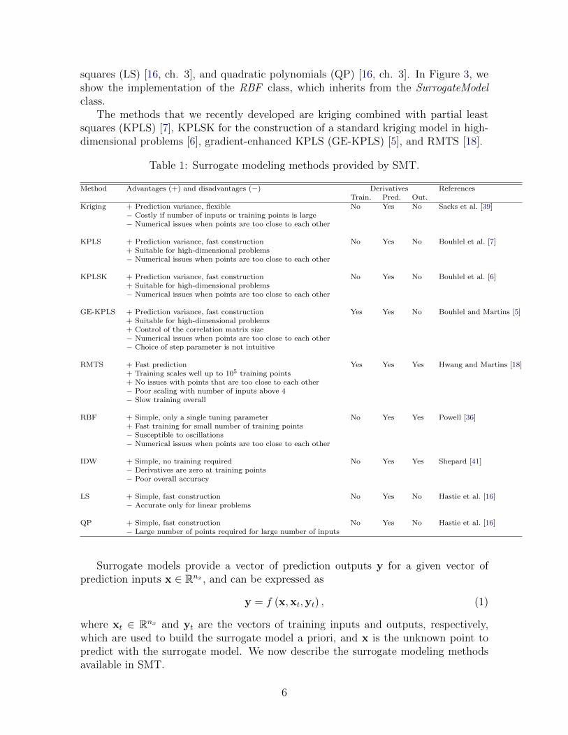
squares (LS) [16, ch. 3], and quadratic polynomials (QP) [16, ch. 3]. In Figure 3, weshow the implementation of the RBF class, which inherits from the SurrogateModelclass.

The methods that we recently developed are kriging combined with partial leastsquares (KPLS) [7], KPLSK for the construction of a standard kriging model in high-dimensional problems [6], gradient-enhanced KPLS (GE-KPLS) [5], and RMTS [18].

Table 1: Surrogate modeling methods provided by SMT.

Method Advantages (+) and disadvantages (−) Derivatives ReferencesTrain. Pred. Out.

Kriging + Prediction variance, flexible No Yes No Sacks et al. [39]− Costly if number of inputs or training points is large− Numerical issues when points are too close to each other

KPLS + Prediction variance, fast construction No Yes No Bouhlel et al. [7]+ Suitable for high-dimensional problems− Numerical issues when points are too close to each other

KPLSK + Prediction variance, fast construction No Yes No Bouhlel et al. [6]+ Suitable for high-dimensional problems− Numerical issues when points are too close to each other

GE-KPLS + Prediction variance, fast construction Yes Yes No Bouhlel and Martins [5]+ Suitable for high-dimensional problems+ Control of the correlation matrix size− Numerical issues when points are too close to each other− Choice of step parameter is not intuitive

RMTS + Fast prediction Yes Yes Yes Hwang and Martins [18]+ Training scales well up to 105 training points+ No issues with points that are too close to each other− Poor scaling with number of inputs above 4− Slow training overall

RBF + Simple, only a single tuning parameter No Yes Yes Powell [36]+ Fast training for small number of training points− Susceptible to oscillations− Numerical issues when points are too close to each other

IDW + Simple, no training required No Yes Yes Shepard [41]− Derivatives are zero at training points− Poor overall accuracy

LS + Simple, fast construction No Yes No Hastie et al. [16]− Accurate only for linear problems

QP + Simple, fast construction No Yes No Hastie et al. [16]− Large number of points required for large number of inputs

Surrogate models provide a vector of prediction outputs y for a given vector ofprediction inputs x ∈ Rnx , and can be expressed as

y = f (x,xt,yt) , (1)

where xt ∈ Rnx and yt are the vectors of training inputs and outputs, respectively,which are used to build the surrogate model a priori, and x is the unknown point topredict with the surrogate model. We now describe the surrogate modeling methodsavailable in SMT.

6

Figure 3: Implementation of the RBF class, which inherits from the SurrogateModelclass.

from smt.surrogate_models.surrogate_model

import SurrogateModel

class RBF(SurrogateModel ):

def _initialize(self):

super(RBF , self). _initialize ()

...

def _setup(self):

options = self.options

...

def _train(self):

self._setup ()

...

def _predict_values(self , x):

"""

Evaluates the model at a set of points.

x : np.ndarray [n_evals , dim]

Evaluation point input values

y (output ): Evaluation point output values

"""

n = x.shape [0]

...

def _predict_derivatives(self , x, kx):

"""

Evaluates the derivatives at a set of points.

x : np.ndarray [n_evals , dim]

Evaluation point input variable values

kx : int

The 0-based index of the input variable with

respect to which derivatives are desired.

dy_dx (output ): Derivative values.

"""

n = x.shape [0]

...

def _predict_output_derivatives(self , x):

"""

Evaluates the output derivatives at a set of points.

x : np.ndarray [n_evals , dim]

Evaluation point input variable values

dy_dyt (output ): Output derivative values.

"""

n = x.shape [0]

...

3.2.1 LS and QP

The LS method [16] fits a linear model with coefficients β = (β0, β1, . . . , βnx), where nxis the number of dimensions, to minimize the residual sum of the squares between theobserved responses in the dataset, and the responses predicted by the linear approxi-mation, i.e.,

minβ||Xβ − y||22, (2)

7

where X =(

1,x(1)T , . . . ,x(nt)T)T

. The vectors in X have (nt × nx + 1) dimensions

and nt is the number of training points. The square polynomial model is given by [16]

y = Xβ + ε, (3)

where ε is a vector of random errors and

X =

1 x(1)1 . . . x

(1)nx x

(1)1 x

(1)2 . . . x

(1)nx−1x

(1)nx x

(1)1

2. . . x

(1)nx

2

...... . . .

...... . . .

......

...

1 x(nt)1 . . . x

(nt)nx x

(nt)1 x

(nt)2 . . . x

(nt)nx−1x

(nt)nx x

(nt)1

2. . . x

(nt)nx

2

. (4)

The vector of estimated polynomial regression coefficients using ordinary LS estimationis

β = XTX−1XTy. (5)

3.2.2 IDW

The IDW model is an interpolating method where the unknown points are calculatedwith a weighted average of the sampling points using [41]

y =

∑nt

i β(x,x

(i)t

)y

(i)t∑nt

i β(x,x

(i)t

) , if x 6= x(i)t ∀i

y(i)t , if x = x

(i)t for some i

, (6)

where x ∈ Rnx is the prediction input vector, y ∈ R is the prediction output, x(i)t ∈ Rnx

is the input vector for the ith training point, and y(i)t ∈ R is the output value for the

ith training point. The weighting function β is defined as

β(x(i),x(j)

)= ||x(i) − x(j)||−p2 , (7)

where p is a positive real number called the power parameter, which must be strictlygreater than one for the derivatives to be continuous.

3.2.3 RBF

The RBF surrogate model [36] represents the interpolating function as a linear combi-nation of basis functions, one for each training point. RBF are named as such becausethe basis functions depend only on the distance from the prediction point to the train-ing point for the basis function. The coefficients of the basis functions are computedduring the training stage. RBF are frequently augmented to global polynomials tocapture the general trends. The prediction equation for RBF is given by

y = p (x) wp +nt∑i

φ(x,x

(i)t

)wr, (8)

8

where x ∈ Rnx is the prediction input vector, y ∈ R is the prediction output, x(i)t ∈ Rnx

is the input vector for the ith training point, p (x) ∈ Rnp is the vector mapping the

polynomial coefficients to the prediction output, φ(x,x

(i)t

)∈ Rnt is the vector mapping

the RBF coefficients to the prediction output, wp ∈ Rnp is the vector of polynomialcoefficients, and wr ∈ Rnt is the vector of RBF coefficients. The coefficients, wp andwr, are computed by solving the following linear augmented Gram system:

φ(x

(1)t ,x

(1)t

). . . φ

(x

(1)t ,x

(nt)t

)p(x

(1)t

)T...

. . ....

...

φ(x

(nt)t ,x

(1)t

). . . φ

(x

(nt)t ,x

(nt)t

)p(x

(nt)t

)Tp(x

(1)t

). . . p

(x

(nt)t

)0

wr1...

wrnt

wp

=

y

(1)t...

y(nt)t

0

. (9)

Only Gaussian basis functions are implemented currently. These can be written asfollows

φ(x(i),x(j)

)= exp

(−||x

(i) − x(j)||22d2

0

), (10)

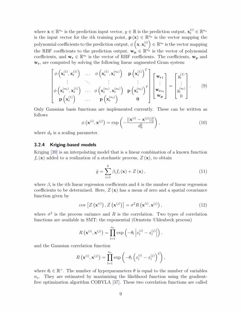
where d0 is a scaling parameter.

3.2.4 Kriging-based models

Kriging [39] is an interpolating model that is a linear combination of a known functionfi (x) added to a realization of a stochastic process, Z (x), to obtain

y =k∑i=1

βifi (x) + Z (x) , (11)

where βi is the ith linear regression coefficients and k is the number of linear regressioncoefficients to be determined. Here, Z (x) has a mean of zero and a spatial covariancefunction given by

cov[Z(x(i)), Z(x(j))]

= σ2R(x(i),x(j)

), (12)

where σ2 is the process variance and R is the correlation. Two types of correlationfunctions are available in SMT: the exponential (Ornstein–Uhlenbeck process)

R(x(i),x(j)

)=

nx∏l=1

exp(−θl

∣∣∣x(i)l − x

(j)l

∣∣∣) ,and the Gaussian correlation function

R(x(i),x(j)

)=

nx∏l=1

exp

(−θl

(x

(i)l − x

(j)l

)2),

where θl ∈ R+. The number of hyperparameters θ is equal to the number of variablesnx. They are estimated by maximizing the likelihood function using the gradient-free optimization algorithm COBYLA [37]. These two correlation functions are called

9

abs exp (exponential) and squar exp (Gaussian) in SMT. The deterministic term, thesum in the kriging prediction (11), is replaced by a constant, a linear model, or aquadratic model, all of which are available in SMT.

KPLS [7] is a kriging model that uses the PLS method. KPLS is faster than krig-ing because fewer hyperparameters need to be estimated to achieve high accuracy.This model is suitable for high-dimensional problems owing to the kernel constructedthrough the PLS method. The PLS method is a well-known tool for high-dimensionalproblems that searches the direction that maximizes the variance between the inputand output variables. This is done by a projection in a smaller space spanned by theprincipal components. The PLS information is integrated into the kriging correlationmatrix to scale the number of inputs by reducing the number of hyperparameters. Thenumber of principal components, h, which corresponds to the number of hyperparam-eters in KPLS is much lower than nx. For example, the PLS-Gaussian correlationfunction is

R(x(i),x(j)

)=

nx∏l=1

h∏k=1

exp

(−θkw(k)2

l

(x

(i)l − x

(j)l

)2). (13)

We provide more details on the KPLS method in previous work [7].The KPLSK model is built in two steps [6]. The first step is to run KPLS and

estimate the hyperparameters expressed in the reduced space with h dimensions. Thesecond step is to express the estimated hyperparameters in the original space with nxdimensions, and then use this as a starting point to optimize the likelihood function ofa standard kriging model. The idea here is to guess a “good” initial hyperparameterand apply a gradient-based optimization using a classic kriging kernel. This guess isprovided by the KPLS construction: the solutions (θ∗1, . . . , θ

∗h) and the PLS-coefficients(

w(k)1 , . . . , w

(k)nx

)for k = 1, . . . , h. Using the change of variables

ηl =h∑k=1

θ∗kw(k)l

2(14)

for l = 1, . . . , nx, we express the initial hyperparameters point in the original space. Wedemonstrate this using a KPLS-Gaussian correlation function RKPLS in the followingexample [6]:

RKPLS

(x(i),x(j)

)=

h∏k=1

nx∏l=1

exp

(−θkw(k)

l

2(x

(i)l − x

(j)l

)2)

= exp

(nx∑l=1

h∑k=1

−θkw(k)l

2(x

(i)l − x

(j)l

)2)

= exp

(nx∑l=1

−ηl(x

(i)l − x

(j)l

)2)

=nx∏l=1

exp

(−ηl

(x

(i)l − x

(j)l

)2),

(15)

10

where the change of variables is performed on the third line, and the last line is astandard Gaussian correlation function. The hyperparameters point (14) provides astarting point for a gradient-based optimization applied on a standard kriging method.

3.2.5 Gradient-enhanced KPLS models

GE-KPLS [5] is a gradient-enhanced kriging (GEK) model with the PLS approach.GEK is an extension of kriging that exploits gradient information. GEK is usually moreaccurate than kriging; however, it is not computationally efficient when the number ofinputs, the number of sampling points, or both, are high. This is primarily owing tothe size of the corresponding correlation matrix that increases in proportion to boththe number of inputs and the number of sampling points.

To address these issues, GE-KPLS exploits the gradient information with a slightincrease in the size of the correlation matrix and reduces the number of hyperparam-eters. The key idea of GE-KPLS is to generate a set of approximating points aroundeach sampling point using a first-order Taylor approximation. Then, the PLS methodis applied several times, each time on a different number of sampling points with theassociated sampling points. Each PLS provides a set of coefficients that contribute toeach variable nearby the associated sampling point to the output. Finally, an average ofall PLS coefficients is computed to estimate the global influence to the output. Denot-

ing these coefficients by(w

(k)1 , . . . , w

(k)nx

), the GE-KPLS Gaussian correlation function

is given by

RGE-KPLS

(x(i),x(j)

)= σ

nx∏l=1

h∏k=1

exp

(−θk

(w

(k)l x

(i)l − w

(k)l x

(j)l

)2). (16)

This approach reduces the number of hyperparameters (reduced dimension) from nxto h, where h << nx.

As mentioned previously, PLS is applied several times with respect to each samplingpoint, which provides the influence of each input variable around that point. The ideahere is to add only m approximating points (m ∈ [1, nx]) around each sampling point.Only the m highest coefficients given by the first principal component are considered,which usually capture the most useful information. Bouhlel and Martins [5] providemore details on this approach.

3.2.6 RMTS method

The RMTS model is a type of surrogate model for low-dimensional problems withlarge datasets that has fast prediction capability [18]. The underlying mathematicalfunctions are tensor-product splines, which limits RMTS to up to four-dimensionalproblems, or five-dimensional problems in certain cases. On the other hand, tensor-product splines enable a fast prediction time that does not increase with the numberof training points. Unlike other methods, such as kriging and RBF, RMTS is notsusceptible to numerical issues when there is a large number of training points or whenpoints are too close together. The prediction equation for RMTS is given by

y = F (x) w, (17)

11

where x ∈ Rnx is the prediction input vector, y ∈ R is the prediction output, w ∈ Rnw

is the vector of spline coefficients, and F (x) ∈ Rnw is the vector mapping the splinecoefficients to the prediction output.

RMTS computes the coefficients of the splines, w, by solving an energy minimiza-tion problem subject to the conditions that the splines pass through the training points.This is formulated as an unconstrained optimization problem where the objective func-tion consists of a term with the second derivatives of the splines, a term that representsthe approximation error for the training points, and another term for regularization.Thus, this optimization problem can be written as

minw

1

2wTHw +

1

2βwTw +

1

2

1

α

nt∑i

[F(x

(i)t

)w − y(i)

t

]2

, (18)

where x(i)t ∈ Rnx is the input vector for the ith training point, y

(i)t ∈ R is the output

value for the ith training point, H ∈ Rnw×nw is the matrix of second derivatives,

F(x

(i)t

)∈ Rnw is the vector mapping the spline coefficients to the ith training output,

and α and β are the regularization coefficients.In problems with a large number of training points relative to the number of spline

coefficients, the energy minimization term is not necessary and can be set to zero bysetting the reg cons option to zero. In problems with a small dataset, the energyminimization is necessary. When the true function has high curvature, the energy min-imization can be counterproductive. This can be addressed by increasing the quadraticapproximation term to one of higher order and using Newton’s method to solve theresulting nonlinear system. The nonlinear formulation is given by

minw

1

2wTHw +

1

2βwTw +

1

2

1

α

nt∑i

[F(x

(i)t

)w − y(i)

t

]p, (19)

where p is the order set by the approx order option. The number of Newton iterationsis specified in the nonlinear maxiter option.

RMTS is implemented in SMT with two choices of splines: B-splines and cubicHermite splines. RMTB uses B-splines with a uniform knot vector in each dimension.The number of B-spline control points and the B-spline order in each dimension areoptions that trade off efficiency and precision of the interpolant. For the cubic Hermitesplines, RMTC divides the domain into tensor-product cubic elements. For adjacentelements, the values and derivatives are continuous. The number of elements in eachdimension is an option that trades off efficiency and precision. B-splines are usually thebetter choice when training time is the most important factor, whereas cubic Hermitesplines are the better choice when the accuracy of the interpolant is most important [18].

3.3 Derivatives

There are three types of derivatives in SMT.

Prediction derivatives ( dy/ dx) are derivatives of predicted outputs with respect tothe inputs at which the model is evaluated. These are computed together with the

12

prediction outputs when the surrogate model is evaluated [26]. These are requiredfor gradient-based optimization algorithms based on surrogate models [2, 3].

Training derivatives ( dyt/ dxt) are derivatives of the training outputs with respectto the corresponding inputs. These are provided by the user and are used toimprove the model accuracy in GE-KPLS.

When the adjoint method is used to compute training derivatives, a high-qualitysurrogate model can be constructed with a low relative cost, because the adjointmethod computes these derivatives at a cost independent of the number of inputs.

Output derivatives ( dy/ dyt) are derivatives of predicted outputs with respect totraining outputs, which is a measure of how the prediction changes with a changein training outputs, accounting for the retraining of the surrogate model. Thesepost-training derivatives are used when the surrogate model is trained within anoptimization iteration. This feature is not commonly available in other frame-works; however, it is required when the training of the surrogate model is embed-ded in a gradient-based optimization. In this case, derivatives of the predictionoutputs with respect to the training outputs must be computed and combinedwith derivatives from other parts of the model using, for example, the chain rule.

Given its focus on derivatives, SMT is synergistic with the OpenMDAO frame-work [14], which is a software framework for gradient-based multidisciplinary analysisand optimization [17, 31, 32]. An SMT surrogate model can be a component that ispart of a larger model developed in OpenMDAO and can provide the derivatives thatOpenMDAO requires from its components to compute the coupled derivatives of themultidisciplinary model.

3.4 Additional surrogate modeling methods

To extend surrogate modeling to higher-level methods, we implemented a componentwithin SMT named extensions. These methods require additional and sometimes dif-ferent steps than the usual surrogate modeling. For example, multi-fidelity methodscombine data generated from different sources, such as coarse and fine mesh solutions.Another example is the mixture of experts (MoE) class of methods, which linearlycombines several surrogates. Three such methods are available within SMT.

MoE modeling performs a weighted sum of local surrogate models (experts) insteadof one single model. It is based on splitting the input space into several subspacesvia clustering algorithms and training a surrogate model within each subspace.Hastie et al. [16] provide a general introduction to the MoE method. The im-plementation of MoE within SMT is based on Gaussian mixture models andexpectation maximization [4].

Variable-fidelity modeling (VFM) samples points using both low-fidelity functionevaluations that are cheap to evaluate and more costly high-fidelity evaluations.It then uses the differences between the high- and low-fidelity evaluations to

13

construct a bridge function that corrects the low-fidelity model [15]. SMT imple-ments additive and multiplicative bridge functions.

Multi-fidelity kriging (MFK) uses a correlation factor ρ(x) (constant, linear, orquadratic) and a discrepancy function δ(x). The high-fidelity model is given by

yhigh(x) = ρ(x)ylow(x) + δ(x).

SMT follows the formulation proposed by Le Gratiet [25], which is recursive andcan be easily extended to multiple levels of fidelity.

4 Example and benchmark functionsSMT contains a library of analytical and engineering problems that can be used for in-structional or benchmarking purposes. The analytical functions currently implementedin SMT are the sphere, Branin, Lp norm, Rosenbrock, and tensor-product functions, allof which are detailed in A. The engineering functions currently implemented in SMTare the cantilever beam, robot arm, torsion vibration, water flow, welded beam, andwing weight problems (described in B).

Figure 4 shows the implementation of the Sphere class, which inherits from theProblem class. This function is a simple example that serves as a good first test fornewly developed surrogate modeling and surrogate-based optimization methods. Thisfunction is a continuous and convex function where the global minimum is at the origin.

Figure 5 shows an example of the use of RMTC within SMT for the robot armfunction [1]. This function is scalable; however, the number of dimensions must be aneven number (we use two dimensions in this example). This function gives the positionof a robot arm, which is made by multiple segments, in a two-dimensional space wherethe shoulder of the arm is fixed at the origin. This function is highly nonlinear, andthe use of training derivatives samples is particularly beneficial in this case [5].

5 ApplicationsIn this section, we describe two applications that highlight the unique features of SMT.We also provide an overview of the main previous applications realized using SMT.The first application is the computation and validation of the prediction derivatives foran airfoil analysis tool, where we apply GE-KPLS. The second application describesa practical use for output derivatives, where we use RMTS to compute the outputsderivatives for a surrogate model that is dynamically trained with an optimizationiteration.

5.1 Airfoil analysis and shape optimization tool

Li et al. [26] used the GE-KPLS implementation in SMT with an MoE technique todevelop a data-driven approach to airfoil and shape optimization based on compu-tational fluid dynamics (CFD) simulations7. They used a database of 1100 existing

7https://github.com/mdolab/adflow

14

Figure 4: Implementation of the Sphere class, which inherits from the Problem class.The main function is evaluate, which computes either the output values or the deriva-tives depending on the variable kx.

import numpy as np

from smt.problems.problem import Problem

class Sphere(Problem ):

# Class Sphere inherits class Problem

# Set up methods of class

def _initialize(self):

self.options.declare(’name’, ’Sphere ’, types=str)

def _setup(self):

# Bornes of the sphere problem

self.xlimits[:, 0] = -10.

self.xlimits[:, 1] = 10.

def _evaluate(self , x, kx):

"""

Arguments

---------

x : ndarray[ne , nx]

Evaluation points.

kx : int or None

Index of derivative (0-based) to return

values with respect to. None means return

function value rather than derivative.

Returns

-------

ndarray[ne, 1]

Functions values if kx=None or derivative

values if kx is an int.

"""

ne, nx = x.shape

y = np.zeros((ne, 1), complex)

if kx is None:

y[:, 0] = np.sum(x**2, 1).T

else:

y[:, 0] = 2 * x[:, kx]

return y

airfoils8 and enriched the database with 100,000 more generated airfoils. The data wasused to create a surrogate model of force coefficients (lift, drag, and moment) withrespect to flight speed (Mach number), the angle of attack, and airfoil shape variables.The shape design variables consisted of shape modes obtained by singular-value de-composition of the existing airfoil shapes. The approach proved successful, enablingshape optimization in 2 sec using a personal computer with an error of less than 0.25%for subsonic flight conditions. This is thousands of times faster than optimization usingdirect calls to CFD.

To validate the prediction derivatives provided by SMT, we built a surrogate modelof the airfoil drag coefficient similar to the one above using the following four inputs:first thickness mode t1, first camber mode c1, Mach number M , and angle of attack α.We compute the partial derivatives of the drag coefficient (Cd) with respect to these

8http://webfoil.engin.umich.edu

15

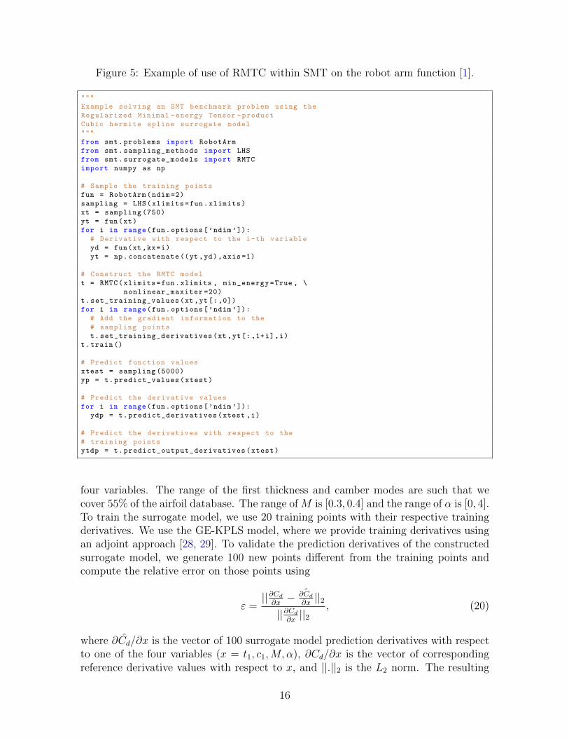
Figure 5: Example of use of RMTC within SMT on the robot arm function [1].

"""

Example solving an SMT benchmark problem using the

Regularized Minimal -energy Tensor -product

Cubic hermite spline surrogate model

"""

from smt.problems import RobotArm

from smt.sampling_methods import LHS

from smt.surrogate_models import RMTC

import numpy as np

# Sample the training points

fun = RobotArm(ndim =2)

sampling = LHS(xlimits=fun.xlimits)

xt = sampling (750)

yt = fun(xt)

for i in range(fun.options[’ndim’]):

# Derivative with respect to the i-th variable

yd = fun(xt,kx=i)

yt = np.concatenate ((yt,yd),axis =1)

# Construct the RMTC model

t = RMTC(xlimits=fun.xlimits , min_energy=True , \

nonlinear_maxiter =20)

t.set_training_values(xt,yt[:,0])

for i in range(fun.options[’ndim’]):

# Add the gradient information to the

# sampling points

t.set_training_derivatives(xt,yt[:,1+i],i)

t.train()

# Predict function values

xtest = sampling (5000)

yp = t.predict_values(xtest)

# Predict the derivative values

for i in range(fun.options[’ndim’]):

ydp = t.predict_derivatives(xtest ,i)

# Predict the derivatives with respect to the

# training points

ytdp = t.predict_output_derivatives(xtest)

four variables. The range of the first thickness and camber modes are such that wecover 55% of the airfoil database. The range of M is [0.3, 0.4] and the range of α is [0, 4].To train the surrogate model, we use 20 training points with their respective trainingderivatives. We use the GE-KPLS model, where we provide training derivatives usingan adjoint approach [28, 29]. To validate the prediction derivatives of the constructedsurrogate model, we generate 100 new points different from the training points andcompute the relative error on those points using

ε =||∂Cd

∂x− ˆ∂Cd

∂x||2

||∂Cd

∂x||2

, (20)

where ∂Cd/∂x is the vector of 100 surrogate model prediction derivatives with respectto one of the four variables (x = t1, c1,M, α), ∂Cd/∂x is the vector of correspondingreference derivative values with respect to x, and ||.||2 is the L2 norm. The resulting

16

relative errors corresponding to each variable (listed in Table 2) show that the surrogatemodel provides an accurate estimate of the derivatives with a relative error less or equalto 10−2.

Table 2: Relative error of the prediction derivative of Cd with respect to t1, c1, M ,and α. The surrogate model yields an accurate prediction derivative with an error lessthan or equal to 10−2.

∂Cd/∂t1 ∂Cd/∂c1 ∂Cd/∂M ∂Cd/∂αε 0.010 0.007 0.009 0.002

Using the constructed surrogate, we compare two gradient-based optimization al-gorithms:

Optimization 1 uses the surrogate model derivatives provided by SMT;

Optimization 2 uses finite-difference derivatives.

The optimization problem is to minimize the drag coefficient (Cd) subject to a liftconstraint (Cl = 0.5). Optimization 1 achieved a slightly lower drag (0.03%) thanOptimization 2 using 21 times fewer evaluations.

CD (10 4) CL Number ofEvaluations

BaselineOptimization 1Optimization 2

99.90 94.57 94.60

0.582 0.500 0.500

--8172

0.1

0.0

0.1

1.0

0.5

0.0

0.5

1.0

Figure 6: Top left: drag and lift coefficients for the baseline, the solution of Optimiza-tion 1, and the solution of Optimization 2. Bottom left: airfoil shapes for all threecases; the shapes for both optimizations is indistinguishable. Right: pressure distri-butions. Optimization 1 achieved a 0.03% lower drag compared with Optimization 2using a fraction of the evaluations.

17

5.2 Aircraft design optimization considering dynamics

The design optimization of commercial aircraft using CFD is typically done by modelingthe aircraft performance at a small number of representative flight conditions [22, 23].This simplification is made because it would be prohibitively expensive to simulatethe full, discretized mission profile using CFD at all points. However, full-missionsimulation is sometimes necessary, such as when the flight is short or when consideringmorphing aircraft designs [9, 30]. This requires a surrogate model of the aerodynamicperformance as a function of a small number of parameters such as flight speed andaltitude. In a design optimization context, the surrogate model must be retrained eachoptimization iteration because the aircraft design changes from iteration to iterationas the shape is being optimized.

This is the situation in an aircraft allocation-mission-design optimization problemrecently solved using RMTS [19]. In this work, the optimization problem maximizedairline profit by optimizing the twist, span, sweep, and shape of the wing of a next-generation commercial aircraft. The profit was computed by simulating the fuel effi-ciency and flight time for the aircraft on a set of routes operated by the hypotheticalairline. To do this, a surrogate model was generated for the wing lift and drag co-efficients (CL and CD) as a function of the angle of attack (α), Mach number (M),and altitude (h). In each optimization iteration, the training CL and CD values werecomputed at a series of points in M–α–h space using CFD. The training outputs wereused to retrain the RMTS surrogate model, and the mission simulations for all theairline routes were performed using inexpensive evaluations of the trained surrogatemodel, as shown in Figure 7. However, because the overall optimization problem wassolved using a gradient-based algorithm, we required derivatives of the prediction out-puts (CL and CD values at the M–α–h points at which we evaluated the surrogate)with respect to the training outputs (CL and CD values at the fixed M–α–h pointswhere the training points were located).

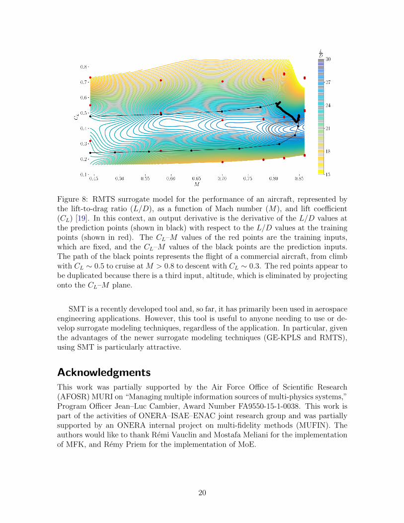
Figure 8 shows the surrogate model with the altitude axis eliminated by projectingonto the other two axes, where CL replaces α as one of the inputs. The horizontal andvertical axes represent the inputs. The red points are the training points and the blackpoints are the prediction points. Therefore, the output derivatives are the derivativesof the outputs at the black points with respect to the training outputs at the red points.

5.3 Other applications

In addition to the two applications we just described, SMT has been used to solve otherengineering problems. We summarize these applications in Table 3. The number ofinput variables ranges from 2 to 99. This demonstrates SMT’s ability to solve differentengineering problems of various complexities.

6 ConclusionsSMT is unique compared with existing surrogate modeling libraries in that it is de-signed from the ground up to handle derivative information effectively. The derivative

18

OptimizerArea, sweep,twist, shape

Area, sweep,twist, shape

Altitude,cruise Mach

Altitude AltitudeAllocationvariables

Geometricconstraints

Geometricmodel

CFD solverCFD training

data

Atmosphericmodels

Mach MachVelocity,density

Aerodynamicsurrogate

Drag

Propulsionsurrogate

SFC

Thrustconstraints

Lift ThrustMission

analysis eq.Fuel burn,block time

Profit, alloc.constraints

Allocationmodel

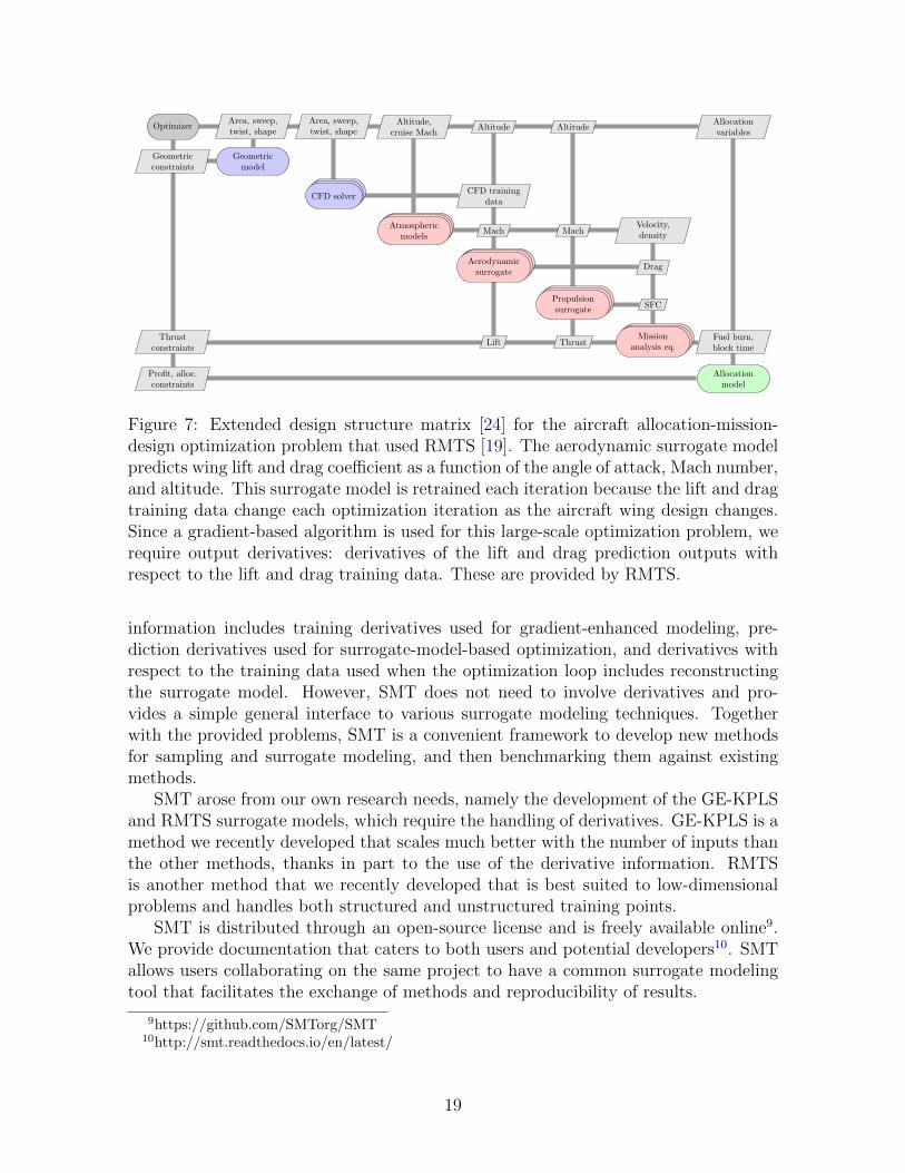
Figure 7: Extended design structure matrix [24] for the aircraft allocation-mission-design optimization problem that used RMTS [19]. The aerodynamic surrogate modelpredicts wing lift and drag coefficient as a function of the angle of attack, Mach number,and altitude. This surrogate model is retrained each iteration because the lift and dragtraining data change each optimization iteration as the aircraft wing design changes.Since a gradient-based algorithm is used for this large-scale optimization problem, werequire output derivatives: derivatives of the lift and drag prediction outputs withrespect to the lift and drag training data. These are provided by RMTS.

information includes training derivatives used for gradient-enhanced modeling, pre-diction derivatives used for surrogate-model-based optimization, and derivatives withrespect to the training data used when the optimization loop includes reconstructingthe surrogate model. However, SMT does not need to involve derivatives and pro-vides a simple general interface to various surrogate modeling techniques. Togetherwith the provided problems, SMT is a convenient framework to develop new methodsfor sampling and surrogate modeling, and then benchmarking them against existingmethods.

SMT arose from our own research needs, namely the development of the GE-KPLSand RMTS surrogate models, which require the handling of derivatives. GE-KPLS is amethod we recently developed that scales much better with the number of inputs thanthe other methods, thanks in part to the use of the derivative information. RMTSis another method that we recently developed that is best suited to low-dimensionalproblems and handles both structured and unstructured training points.

SMT is distributed through an open-source license and is freely available online9.We provide documentation that caters to both users and potential developers10. SMTallows users collaborating on the same project to have a common surrogate modelingtool that facilitates the exchange of methods and reproducibility of results.

9https://github.com/SMTorg/SMT10http://smt.readthedocs.io/en/latest/

19

Initial design

Optimized design

Fig. 8 The contours show L/D, the red markers indicate training point locations, and the black markers andlines indicate the path of the aircraft through CL-M space for the longest-range mission. The L/D = 26 contouris highlighted in grey.

22

Figure 8: RMTS surrogate model for the performance of an aircraft, represented bythe lift-to-drag ratio (L/D), as a function of Mach number (M), and lift coefficient(CL) [19]. In this context, an output derivative is the derivative of the L/D values atthe prediction points (shown in black) with respect to the L/D values at the trainingpoints (shown in red). The CL–M values of the red points are the training inputs,which are fixed, and the CL–M values of the black points are the prediction inputs.The path of the black points represents the flight of a commercial aircraft, from climbwith CL ∼ 0.5 to cruise at M > 0.8 to descent with CL ∼ 0.3. The red points appear tobe duplicated because there is a third input, altitude, which is eliminated by projectingonto the CL–M plane.

SMT is a recently developed tool and, so far, it has primarily been used in aerospaceengineering applications. However, this tool is useful to anyone needing to use or de-velop surrogate modeling techniques, regardless of the application. In particular, giventhe advantages of the newer surrogate modeling techniques (GE-KPLS and RMTS),using SMT is particularly attractive.

AcknowledgmentsThis work was partially supported by the Air Force Office of Scientific Research(AFOSR) MURI on “Managing multiple information sources of multi-physics systems,”Program Officer Jean–Luc Cambier, Award Number FA9550-15-1-0038. This work ispart of the activities of ONERA–ISAE–ENAC joint research group and was partiallysupported by an ONERA internal project on multi-fidelity methods (MUFIN). Theauthors would like to thank Remi Vauclin and Mostafa Meliani for the implementationof MFK, and Remy Priem for the implementation of MoE.

20

Table 3: Summary of SMT applications to engineering design problems.

Problem Surrogate Objective of the study Number of Referenceused design variables

3D blade KPLS Compare the accuracy and efficiency of the Up to 99 Bouhlel et al. [7]KPLS model and the Optimus [34]implementation of the kriging model

3D blade KPLSK Compare the accuracy and efficiency of the 99 Bouhlel et al. [6]KPLSK model and the KPLS model

Automotive KPLS, Minimize the mass of a vehicle subject to 50 Bouhlel et al. [8]KPLSK 68 constraints

Eight different GE-KPLS Compare the accuracy and efficiency of the Up to 15 Bouhlel and Martins [5]engineering GE-KPLS model and the indirect GEKproblems

Aircraft wing MoE Minimize the drag of aircraft wings subject Up to 17 Bartoli et al. [2]to lift constraints

2D airfoils GE-KPLS Build a fast interactive airfoil analysis and Up to 16 Li et al. [26]design optimization tool

Aircraft RMTS Optimize an aircraft design while analyzing 3 Hwang and Munster [19]performance the full mission using a CFD surrogate

Rotor RMTS Optimize a rotor using a surrogate model 2 Hwang and Ning [20]analysis for the lift and drag of blade airfoils

A Analytical functions implemented in SMTIn the following descriptions, nx is the number of dimensions.

Sphere The sphere function is quadratic, continuous, convex, and unimodal. It isgiven by

nx∑i=1

x2i , −10 ≤ xi ≤ 10, for i = 1, . . . , nx.

Branin [12] The Branin function is commonly used in optimization and has threeglobal minima. It is given by

f (x) =

(x2 −

5.1

4π2x2

1 +5

πx1 − 6

)2

+ 10

(1− 1

8π

)cos (x1) + 10,

where x = (x1, x2) with −5 ≤ x1 ≤ 10 and 0 ≤ x2 ≤ 15.

Rosenbrock [40] The Rosenbrock function is a continuous, nonlinear, and non-convex function and usually used in optimization. The minimum of this function issituated in a parabolic-shaped flat valley and is given by

nx−1∑i=1

[(xi+1 − x2

i

)2+ (xi − 1)2

], −2 ≤ xi ≤ 2, for i = 1, . . . , nx.

21

Tensor-product The tensor-product function approximates a step function, whichcauses oscillations with some surrogate models [18], and is given by

nx∏i=1

cos (aπxi) , −1 ≤ xi ≤ 1, for i = 1, . . . , nx,

ornx∏i=1

exp (xi) , −1 ≤ xi ≤ 1, for i = 1, . . . , nx,

ornx∏i=1

tanh (xi) , −1 ≤ xi ≤ 1, for i = 1, . . . , nx,

ornx∏i=1

exp(−2x2

i

), −1 ≤ xi ≤ 1, for i = 1, . . . , nx.

B Engineering problems implemented in SMT

Cantilever beam [10]

This function models a simple uniform cantilever beam with vertical and horizontalloads

50

600

17∑i=1

12

bih3i

( 17∑j=i

lj

)3

−

(17∑

j=i+1

lj

)3 ,

where bi ∈ [0.01, 0.05], hi ∈ [0.3, 0.65], li ∈ [0.5, 1].

Robot arm [1]

This function gives the position of a robot arm√√√√( 4∑i=1

Li cos

(i∑

j=1

θj

))2

+

(4∑i=1

Li sin

(i∑

j=1

θj

))2

,

where Li ∈ [0, 1] for i = 1, . . . , 4 and θj ∈ [0, 2π] for j = 1, . . . , 4.

Torsion vibration [27]

This function gives the low natural frequency of a torsion problem

1

2π

√−b−

√b2 − 4ac

2a,

where Ki = πGidi32Li

, Mj =ρjπtjDj

4g, Jj = 0.5Mj

Dj

2, a = 1, b = −

(K1+K2J1

+ K2+K3J2

),

c = K1K2+K2K3+K3K1

J1J2, for d1 ∈ [1.8, 2.2], L1 ∈ [9, 11], G1 ∈ [105300000, 128700000],

22

d2 ∈ [1.638, 2.002], L2 ∈ [10.8, 13.2], G2 ∈ [5580000, 6820000], d3 ∈ [2.025, 2.475], L3 ∈[7.2, 8.8], G3 ∈ [3510000, 4290000], D1 ∈ [10.8, 13.2], t1 ∈ [2.7, 3.3], ρ1 ∈ [0.252, 0.308],D2 ∈ [12.6, 15.4], t2 ∈ [3.6, 4.4], and ρ1 ∈ [0.09, 0.11].

Water flow [33]

This function characterizes the flow of water through a borehole that is drilled fromthe ground surface through two aquifers

2πTu (Hu −Hl)

ln(

rrw

)[1 + 2LTu

ln( rrw

)r2wKw+ Tu

Tl

] ,where 0.05 ≤ rw ≤ 0.15, 100 ≤ r ≤ 50000, 63070 ≤ Tu ≤ 115600, 990 ≤ Hu ≤ 1110,63.1 ≤ Tl ≤ 116, 700 ≤ Hl ≤ 820, 1120 ≤ L ≤ 1680, and 9855 ≤ Kw ≤ 12045.

Welded beam [11]

The shear stress of a welded beam problem is given by√τ ′2 + τ ′′2 + lτ ′τ ′′√0.25 (l2 + (h+ t)2)

,

where τ ′ = 6000√2hl

, τ ′′ =6000(14+0.5l)

√0.25(l2+(h+t)2)

2[0.707hl

(l2

12+0.25(h+t)2

)] , for h ∈ [0.125, 1], and l, t ∈ [5, 10].

Wing weight [12]

The estimate of the weight of a light aircraft wing is given by

0.036S0.758w W 0.0035

fw

(A

cos2 Λ

)q0.006λ0.04

(100tc

cos Λ

)−0.3

(NzWdg)0.49 + SwWp,

where 150 ≤ Sw ≤ 200, 220 ≤ Wfw ≤ 300, 6 ≤ A ≤ 10, −10 ≤ Λ ≤ 10, 16 ≤ q ≤ 45,0.5 ≤ λ ≤ 1, 0.08 ≤ tc ≤ 0.18, 2.5 ≤ Nz ≤ 6, 1700 ≤ Wdg ≤ 25000, and 0.025 ≤ Wp ≤0.08.

References[1] J. An and A. Owen. Quasi-regression. Journal of Complexity, 17(4):588–607, 2001.

ISSN 0885-064X. doi:10.1006/jcom.2001.0588.

[2] N. Bartoli, T. Lefebvre, S. Dubreuil, R. Olivanti, N. Bons, J. R. R. A. Martins,M. A. Bouhlel, and J. Morlier. An adaptive optimization strategy based on mixtureof experts for wing aerodynamic design optimization. In Proceedings of the 18thAIAA/ISSMO Multidisciplinary Analysis and Optimization Conference, Denver,CO, June 2017. doi:10.2514/6.2017-4433.

23

[3] N. Bartoli, T. Lefebvre, S. Dubreuil, R. Olivanti, R. Priem, N. Bons, J. R. R. A.Martins, and J. Morlier. Adaptive modeling strategy for constrained global op-timization with application to aerodynamic wing design. Aerospace Science andTechnology, 2019. (In press).

[4] D. Bettebghor, N. Bartoli, S. Grihon, J. Morlier, and M. Samuelides. Surro-gate modeling approximation using a mixture of experts based on em joint es-timation. Structural and Multidisciplinary Optimization, 43(2):243–259, 2011.10.1007/s00158-010-0554-2.

[5] M. A. Bouhlel and J. R. R. A. Martins. Gradient-enhanced kriging for high-dimensional problems. Engineering with Computers, 1(35):157–173, January 2019.doi:10.1007/s00366-018-0590-x.

[6] M. A. Bouhlel, N. Bartoli, J. Morlier, and A. Otsmane. An improved approach forestimating the hyperparameters of the kriging model for high-dimensional prob-lems through the partial least squares method. Mathematical Problems in Engi-neering, 2016. doi:10.1155/2016/6723410. Article ID 6723410.

[7] M. A. Bouhlel, N. Bartoli, A. Otsmane, and J. Morlier. Improving kriging sur-rogates of high-dimensional design models by partial least squares dimensionreduction. Structural and Multidisciplinary Optimization, 53(5):935–952, 2016.doi:10.1007/s00158-015-1395-9.

[8] M. A. Bouhlel, N. Bartoli, R. G. Regis, A. Otsmane, and J. Morlier. Efficientglobal optimization for high-dimensional constrained problems by using the krigingmodels combined with the partial least squares method. Engineering Optimization,50(12):2038–2053, 2018. doi:10.1080/0305215X.2017.1419344.

[9] D. A. Burdette and J. R. R. A. Martins. Impact of morphing trailing edge onmission performance for the common research model. Journal of Aircraft, 56(1):369–384, January 2019. doi:10.2514/1.C034967.

[10] G. H. Cheng, A. Younis, K. H. Hajikolaei, and G. G. Wang. Trust region basedmode pursuing sampling method for global optimization of high dimensional de-sign problems. Journal of Mechanical Design, 137(2):021407, 2015.

[11] K. Deb. An efficient constraint handling method for genetic algorithms. Com-puter Methods in Applied Mechanics and Engineering, 186(2–4):311–338, 1998.doi:10.1016/S0045-7825(99)00389-8.

[12] A. I. J. Forrester, A. Sobester, and A. J. Keane. Engineering Design via SurrogateModelling—A Practical Guide. Wiley, 2008. ISBN 978-0-470-06068-1.

[13] D. Gorissen, K. Crombecq, I. Couckuyt, T. Dhaene, and P. Demeester. A surrogatemodeling and adaptive sampling toolbox for computer based design. Journal ofMachine Learning Research, 11:2051–2055, July 2010.

24

[14] J. S. Gray, J. T. Hwang, J. R. R. A. Martins, K. T. Moore, and B. A. Nay-lor. OpenMDAO: An open-source framework for multidisciplinary design, anal-ysis, and optimization. Structural and Multidisciplinary Optimization, 2019.doi:10.1007/s00158-019-02211-z. (In press).

[15] Z.-H. Han, S. Gortz, and R. Zimmermann. Improving variable-fidelity surro-gate modeling via gradient-enhanced kriging and a generalized hybrid bridgefunction. Aerospace Science and Technology, 25(1):177–189, March 2013.doi:10.1016/j.ast.2012.01.006.

[16] T. Hastie, R. Tibshirani, and J. Friedman. The Elements of Statistical Learning.Springer Series in Statistics. Springer New York Inc., New York, NY, USA, 2001.

[17] J. T. Hwang and J. R. R. A. Martins. A computational architecture forcoupling heterogeneous numerical models and computing coupled derivatives.ACM Transactions on Mathematical Software, 44(4):Article 37, June 2018.doi:10.1145/3182393.

[18] J. T. Hwang and J. R. R. A. Martins. A fast-prediction surrogate modelfor large datasets. Aerospace Science and Technology, 75:74–87, April 2018.doi:10.1016/j.ast.2017.12.030.

[19] J. T. Hwang and D. W. Munster. Solution of ordinary differential equations ingradient-based multidisciplinary design optimization. In 2018 AIAA/ASCE/AH-S/ASC Structures, Structural Dynamics, and Materials Conference, Kissimmee,FL, January 2018. AIAA, AIAA. doi:10.2514/6.2018-1646.

[20] J. T. Hwang and A. Ning. Large-scale multidisciplinary optimization of an electricaircraft for on-demand mobility. In 2018 AIAA/ASCE/AHS/ASC Structures,Structural Dynamics, and Materials Conference, Kissimmee, FL, January 2018.doi:10.2514/6.2018-1384.

[21] R. Jin, W. Chen, and A. Sudjianto. An efficient algorithm for constructing optimaldesign of computer experiments. Journal of Statistical Planning and Inference, 134(1):268–287, September 2005. ISSN 0378-3758. doi:10.1016/j.jspi.2004.02.014.

[22] G. K. W. Kenway and J. R. R. A. Martins. Multipoint high-fidelity aerostructuraloptimization of a transport aircraft configuration. Journal of Aircraft, 51(1):144–160, January 2014. doi:10.2514/1.C032150.

[23] G. K. W. Kenway and J. R. R. A. Martins. Multipoint aerodynamic shape opti-mization investigations of the Common Research Model wing. AIAA Journal, 54(1):113–128, January 2016. doi:10.2514/1.J054154.

[24] A. B. Lambe and J. R. R. A. Martins. Extensions to the design structure matrixfor the description of multidisciplinary design, analysis, and optimization pro-cesses. Structural and Multidisciplinary Optimization, 46:273–284, August 2012.doi:10.1007/s00158-012-0763-y.

25

[25] L. Le Gratiet. Multi-fidelity Gaussian process regression for computer experiments.Theses, Universite Paris–Diderot - Paris VII, Oct. 2013. URL https://tel.

archives-ouvertes.fr/tel-00866770.

[26] J. Li, M. A. Bouhlel, and J. R. R. A. Martins. Data-based approach for fastairfoil analysis and optimization. Journal of Aircraft, 57(2):581–596, February2019. doi:10.2514/1.J057129.

[27] W. Liping, B. Don, W. Gene, and R. Mahidhar. A comparison of metamodelingmethods using practical industry requirements. Proceedings of the 47th AIAA/AS-ME/ASCE/AHS/ASC Structures, Structural Dynamics, and Materials Confer-ence, Newport, RI, 2006.

[28] Z. Lyu, G. K. Kenway, C. Paige, and J. R. R. A. Martins. Automatic differentia-tion adjoint of the Reynolds-averaged Navier–Stokes equations with a turbulencemodel. In 21st AIAA Computational Fluid Dynamics Conference, San Diego, CA,July 2013. doi:10.2514/6.2013-2581.

[29] C. A. Mader, J. R. R. A. Martins, J. J. Alonso, and E. van der Weide. ADjoint:An approach for the rapid development of discrete adjoint solvers. AIAA Journal,46(4):863–873, Apr. 2008. doi:10.2514/1.29123.

[30] J. R. R. A. Martins. Encyclopedia of Aerospace Engineering, volume Green Avi-ation, chapter Fuel burn reduction through wing morphing, pages 75–79. Wiley,October 2016. ISBN 978-1-118-86635-1. doi:10.1002/9780470686652.eae1007.

[31] J. R. R. A. Martins and J. T. Hwang. Review and unification of methods forcomputing derivatives of multidisciplinary computational models. AIAA Journal,51(11):2582–2599, November 2013. doi:10.2514/1.J052184.

[32] J. R. R. A. Martins and A. B. Lambe. Multidisciplinary design optimization:A survey of architectures. AIAA Journal, 51(9):2049–2075, September 2013.doi:10.2514/1.J051895.

[33] M. D. Morris, T. J. Mitchell, and D. Ylvisaker. Bayesian design and analysis ofcomputer experiments: Use of derivatives in surface prediction. Technometrics,35(3):243–255, 1993.

[34] Noesis Solutions. OPTIMUS. 2009. URL http://www.noesissolutions.com/

Noesis/optimus-details/optimus-design-optimization.

[35] F. Pedregosa, G. Varoquaux, A. Gramfort, V. Michel, B. Thirion, O. Grisel,M. Blondel, P. Rettenhofer, R. Weiss, V. Dubourg, J. Vanderplas, A. Passos,D. Cournapeau, M. Brucher, M. Perrot, and E. Duchesnay. Scikit-learn: Machinelearning in Python. Journal of Machine Learning Research, 12:2825–2830, 2011.

[36] M. J. D. Powell. The Theory of Radial Basis Function Approximation in 1990,pages 105–210. Oxford University Press, May 1992.

26

[37] M. J. D. Powell. A Direct Search Optimization Method That Models the Ob-jective and Constraint Functions by Linear Interpolation, pages 51–67. SpringerNetherlands, Dordrecht, 1994. ISBN 978-94-015-8330-5. doi:10.1007/978-94-015-8330-5 4.

[38] C. E. Rasmussen and C. K. I. Williams. Gaussian Processes for Machine Learning.Adaptive Computation and Machine Learning. MIT Press, Cambridge, MA, USA,Jan. 2006.

[39] J. Sacks, S. B. Schiller, and W. J. Welch. Designs for computer experiments.Technometrics, 31(1):41–47, 1989.

[40] Y. Shang and Y. Qiu. A note on the extended Rosenbrock func-tion. Evolutionary Compuation, 14(1):119–126, Mar. 2006. ISSN 1063-6560.doi:10.1162/106365606776022733.

[41] D. Shepard. A two-dimensional interpolation function for irregularly-spaced data.In Proceedings of the 1968 23rd ACM National Conference, ACM ’68, pages 517–524, New York, NY, USA, 1968. ACM. doi:10.1145/800186.810616.

27