Jacobi rational–Gauss collocation method for Lane–Emden ... · [email protected] cFaculty...

Nonlinear Analysis: Modelling and Control, 2014, Vol. 19, No. 4, 537–550 537http://dx.doi.org/10.15388/NA.2014.4.1

Jacobi rational–Gauss collocation methodfor Lane–Emden equations of astrophysical significance

Eid H. Dohaa, Ali H. Bhrawyb,c, Ramy M. Hafezd, Robert A. Van Gordere,1

aFaculty of Science, Cairo UniversityGiza, [email protected] of Science, King Abdulaziz UniversityJeddah, Saudi [email protected] of Science, Beni-Suef UniversityBeni-Suef, EgyptdInstitute of Information Technology, Modern AcademyCairo, [email protected] of Mathematics, University of Central FloridaOrlando, FL 32816, [email protected]

Received: 24 July 2013 / Revised: 22 January 2014 / Published online: 25 August 2014

Abstract. In this paper, a new spectral collocation method is applied to solve Lane–Emdenequations on a semi-infinite domain. The method allows us to overcome difficulty in boththe nonlinearity and the singularity inherent in such problems. This Jacobi rational–Gaussmethod, based on Jacobi rational functions and Gauss quadrature integration, is implementedfor the nonlinear Lane–Emden equation. Once we have developed the method, numerical resultsare provided to demonstrate the method. Physically interesting examples include Lane–Emdenequations of both first and second kind. In the examples given, by selecting relatively few Jacobirational–Gauss collocation points, we are able to get very accurate approximations, and we are thusable to demonstrate the utility of our approach over other analytical or numerical methods. In thisway, the numerical examples provided demonstrate the accuracy, efficiency, and versatility of themethod.

Keywords: Lane–Emden equation, isothermal gas spheres, collocation method, Jacobi rational–Gauss quadrature, Jacobi rational polynomials.

1The author supported in part by NSF grant # 1144246.

c© Vilnius University, 2014

mailto:[email protected]




538 E.H. Doha et al.

1 Introduction

The fundamental goal of this paper is to develop a suitable way to approximate thesingular nonlinear Lane–Emden equation on the interval x ∈ (0,∞) using the Jacobirational polynomials. To this end, consider

u′′(x) +a

xu′ = g

(x, u(x)

), 0 < x <∞, (1)

subject to u(0) = b0 and u′(0) = b1, where the prime denotes differentiation with respectto x, and a > 0, b0 and b1 are constants. Lane–Emden equations model many phenomenain mathematical physics and astrophysics. This equation is a generalization of some ofthe basic equations in the theory of stellar structure, and has been the focus of manystudies [1–7]. When a = 2 and g = um, we recover the Lane–Emden equation of the firstkind, while when g = exp(u), we recover the Lane–Emden equation of the second kind.

Many mathematical problems arising in science and engineering are defined overunbounded domains. To make matters more complicated, many such problems are non-linear. Several spectral methods have been successfully applied in the approximation ofproblems on unbounded domains. The common methods for dealing with such problemsare the Hermite spectral method [8, 9], the Laguerre spectral method [10–12], mappingthe original problem in an unbounded domain to a problem in a bounded domain [13, 14]and rational approximations [15–17].

The solution of nonlinear singular initial value problems of Lane–Emden type isnumerically challenging because of the singularity at the origin, in addition to the strongnonlinearity. Approximate solutions to the Lane–Emden equation were given by implicitseries solution [18] and the homotopy perturbation method [19,20]. In [21], the Boubakerpolynomials expansion scheme is applied successfully in order to obtain analytical-nu-merical solutions for two kind of Lane–Emden problems. The enhanced Lagrangian for-mulation method and the Boubaker polynomials expansion scheme have been confirmedin [22] to solve the related generalized Lane–Emden equation for polytropic star structureanalysis under Bonnor–Ebert gas sphere astrophysical configuration. Moreover, Danishet al. [23] introduced an optimal homotopy analysis method to overcome the presence ofsingularity of some related boundary value problems arising in engineering and appliedsciences.

Polynomial approximations can be quite useful for expressing the solution of a dif-ferential equation [24]. One such approach would be the spectral methods. A well-knownadvantage of a spectral method is that it achieves high accuracy with relatively fewerspatial grid points when compared with other numerical or analytical methods. Recently,Bhrawy et al. [25] proposed the shifted Jacobi collocation spectral method for solvingthe nonlinear Lane–Emden type equation, while the spatial approximation is based onshifted Jacobi polynomials with their parameters α and β and used the collocation nodesof shifted Jacobi–Gauss points. Adibi and Rismani [26] proposed an approximation al-gorithm for the solution of (1) using modified Legendre-spectral method. Recently, thesinc-collocation method and Hermite function collocation method is introduced in [27]and [28] for the solution of Lane–Emden type equations. A modified generalized Laguerre

www.mii.lt/NA

Jacobi rational–Gauss collocation method for Lane–Emden equations 539

functions Lagrangian method and the rational Legendre pseudospectral approach are alsointroduced in [29, 30]. More recently, Pandey et al. [31], and Pandey and Kumar [32] de-veloped two numerical methods for solving Lane–Emden type equations using Legendreand Bernstein operational matrices of differentiation, respectively.

The use of Jacobi polynomials for solving differential equations has gained increasingpopularity in recent years (see [33–37]). The main concern of this paper is to developa spectral Jacobi rational–Gauss collocation (JRC) method to find an approximate solutionuN (x) of singular Lane–Emden type initial value problems on the semi-infinite domain(0,∞). We first derive an algorithm for the general Lane–Emden model so that we mayapply the Jacobi rational–Gauss collocation method to determine solutions. Then weapply the algorithm to some physically reasonable examples, namely, the Lane–Emdenequations of first and second kind, in order to demonstrate the method. We show that theproposed method is both accurate and efficient compared with alternative methods.

This paper is organized as follows. In Section 2, we construct collocation algorithmfor Lane–Emden equation using the Jacobi rational polynomials. Then, in Section 3, theproposed method is applied to various types of Lane–Emden equations, and the results arecompared with existing analytic or exact solutions that were reported in other publishedworks in the literature.

2 Jacobi rational–Gauss collocation method

In this section, we use the Jacobi rational–Gauss collocation method to solve numericallythe following model problem:

u′′(x) = f(x, u(x), u′(x)

), 0 < x <∞, (2)

subject tou(0) = d0, u′(0) = d1, (3)

where the values of d0 and d1 describe the initial state of u(x) and f(x, u, u′) is a non-linear function of x, u and u′ which may be singular at x = 0. It is well known that theLane–Emden equations of first and second kind are special cases of (2)–(3).

It should be noted that for a second-order differential equation with the singularityat x = 0 in the interval [0,∞), one is unable to apply the collocation method withJacobi rational–Gauss–Radau points because the fixed node x = 0 is necessary to use asa collocation node. Therefore, the collocation method with Jacobi rational–Gauss nodesare used to overcome the difficulty of such a singular point at x = 0; i.e., we collocatethe singular nonlinear ODE only at the N − 1 Jacobi Rational–Gauss points that are theN − 1 zeros of the Jacobi rational polynomial on (0,∞). These equations together withtwo initial conditions generate N + 1 nonlinear algebraic equations which can be solved.

Let us first introduce some basic notation that will be used. To begin with, somemathematical preliminaries are laid out in the Appendix. We use the results presentedthere to construct our algorithm. To begin with, we set

SN (0,∞) = span{R

(α,β)0 (x), R

(α,β)1 (x), . . . , R

(α,β)N (x)

}, (4)

Nonlinear Anal. Model. Control, 2014, Vol. 19, No. 4, 537–550


while we define the discrete inner product and norm as

(u, v)χ(α,β)R ,N

=

N∑j=0

u(x(α,β)R,N,j

)v(x(α,β)R,N,j

)$

(α,β)R,N,j ,

‖u‖χ(α,β)R ,N

=√

(u, u)χ(α,β)R ,N

.

(5)

Here x(α,β)R,N,j and $(α,β)R,N,j are the nodes and the corresponding weights of the Jacobi

rational–Gauss quadrature formula on the interval (0,∞), respectively. Obviously,

(u, v)χ(α,β)R ,N

= (u, v)χ(α,β)R

∀u, v ∈ S2N−1. (6)

Thus, for any u ∈ SN (0,∞), the norms ‖u‖χ(α,β)R ,N

and ‖u‖χ(α,β)R

coincide.

Associating with this quadrature rule, we denote by IR(α,β)T

N the Jacobi rational–Gaussinterpolation

IR

(α,β)T

N u(x(α,β)R,N,j

)= u

(x(α,β)R,N,j

), 0 6 k 6 N.

The Jacobi rational–Gauss collocation method for solving (2) and (3) is to seekuN (x) ∈ SN (0,∞) such that

u′′(x(α,β)R,N,k

)= f

(x(α,β)R,N,k, u

(x(α,β)R,N,k), u′

(x(α,β)R,N,k

)), k = 0, 1, . . . , N − 2,

u(i)N (0) = di, i = 0, 1.

(7)

Now, we derive the algorithm for solving the singular second-order differential equa-tion (2) and (3). Let

uN (x) =

N∑j=0

ajR(α,β)j (x), a = (a0, a1, . . . , aN )T. (8)

We first approximate u(x), u′(x) and u′′(x), as Eq. (8). By substituting these approxi-mations in Eq. (2), we get

N∑j=0

ajD2R

(α,β)j (x) = f

(x,

N∑j=0

ajR(α,β)j (x),

N∑j=0

ajDR(α,β)j (x)

). (9)

Therefore, we deduce from (A.11) and (A.12) that

N∑j=0

aj[(j + α+ β + 1)2(x+ 1)−4R

(α+2,β+2)j−2 (x)

− 2(j + α+ β + 1)(x+ 1)−3R(α+1,β+1)j−1 (x)

]= f

(x,

N∑j=0

ajR(α,β)j (x),

N∑j=0

aj(j + α+ β + 1)(x+ 1)−2R(α+1,β+1)j−1 (x)

). (10)

www.mii.lt/NA


Substitution of (8) into (3) yields

N∑j=0

ajDiR

(α,β)j (0) = di, i = 0, 1. (11)

To find the solution uN (x), we first collocate Eq. (10) at the N − 1 Jacobi rationalroots, yields

N∑j=0

aj[(j + α+ β + 1)2

(x(α,β)R,N,k + 1

)−4R

(α+2,β+2)j−2

(x(α,β)R,N,k

)− 2(j + α+ β + 1)

(x(α,β)R,N,k + 1)−3R

(α+1,β+1)j−1

(x(α,β)R,N,k

)]= f

(x(α,β)R,N,k,

N∑j=0

ajR(α,β)j

(x(α,β)R,N,k

),

N∑j=0

aj(j + α+ β + 1)(x(α,β)R,N,k + 1

)−2R

(α+1,β+1)j−1

(x(α,β)R,N,k

)). (12)

Next, Eq. (11), after using (A.9) and (A.10), can be written as

N∑j=0

(−1)jΓ(j + β + 1)

Γ(β + 1)j!aj = d0, (13)

N∑j=1

(−1)j−1(j + α+ β + 1)Γ(j + β + 1)

(j − 1)! Γ(β + 2)aj = d1. (14)

Finally, from (12), (13) and (14), we get N + 1 nonlinear algebraic equations which canbe solved for the unknown coefficients aj by using any standard iteration technique, likeNewton’s iteration method. Consequently, uN (x) given in Eq. (8) can be evaluated.

3 Numerical results

We report in this section some numerical results obtained with the algorithms presentedin the previous section. Comparisons of the results obtained by the present method withthose obtained by other methods reveal that the present method is very accurate andefficient. We consider the two examples, both of which are physically relevant.

3.1 Lane–Emden equation of the first kind

The nonlinear problem we shall consider is the Lane–Emden equation of the first kind, ofindex m. The equation is given by

u′′(x) +2

xu′(x) + um(x) = 0, x > 0, (15)



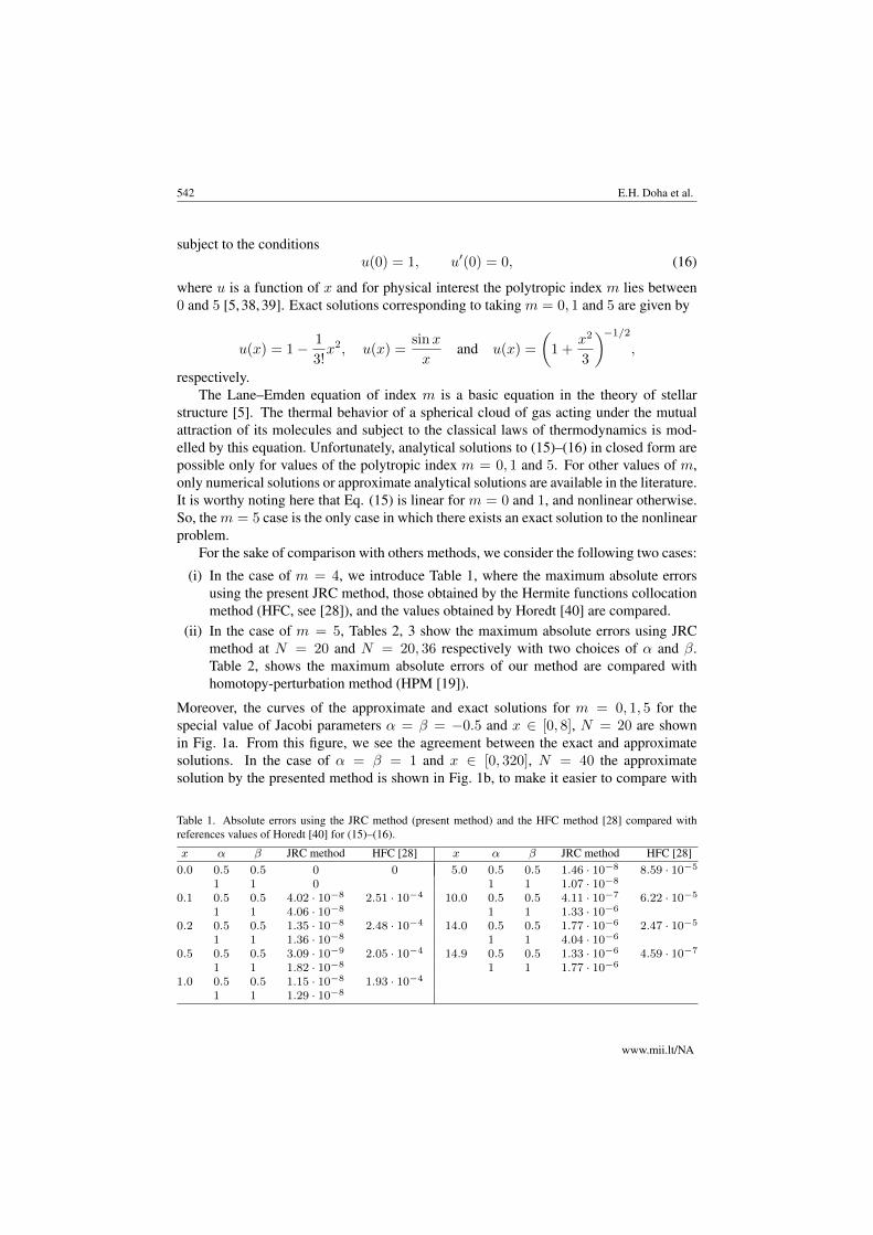
subject to the conditionsu(0) = 1, u′(0) = 0, (16)

where u is a function of x and for physical interest the polytropic index m lies between0 and 5 [5, 38, 39]. Exact solutions corresponding to taking m = 0, 1 and 5 are given by

u(x) = 1− 1

3!x2, u(x) =

sinx

xand u(x) =

(1 +

x2

3

)−1/2,

respectively.The Lane–Emden equation of index m is a basic equation in the theory of stellar

structure [5]. The thermal behavior of a spherical cloud of gas acting under the mutualattraction of its molecules and subject to the classical laws of thermodynamics is mod-elled by this equation. Unfortunately, analytical solutions to (15)–(16) in closed form arepossible only for values of the polytropic index m = 0, 1 and 5. For other values of m,only numerical solutions or approximate analytical solutions are available in the literature.It is worthy noting here that Eq. (15) is linear for m = 0 and 1, and nonlinear otherwise.So, them = 5 case is the only case in which there exists an exact solution to the nonlinearproblem.

For the sake of comparison with others methods, we consider the following two cases:

(i) In the case of m = 4, we introduce Table 1, where the maximum absolute errorsusing the present JRC method, those obtained by the Hermite functions collocationmethod (HFC, see [28]), and the values obtained by Horedt [40] are compared.

(ii) In the case of m = 5, Tables 2, 3 show the maximum absolute errors using JRCmethod at N = 20 and N = 20, 36 respectively with two choices of α and β.Table 2, shows the maximum absolute errors of our method are compared withhomotopy-perturbation method (HPM [19]).

Moreover, the curves of the approximate and exact solutions for m = 0, 1, 5 for thespecial value of Jacobi parameters α = β = −0.5 and x ∈ [0, 8], N = 20 are shownin Fig. 1a. From this figure, we see the agreement between the exact and approximatesolutions. In the case of α = β = 1 and x ∈ [0, 320], N = 40 the approximatesolution by the presented method is shown in Fig. 1b, to make it easier to compare with

Table 1. Absolute errors using the JRC method (present method) and the HFC method [28] compared withreferences values of Horedt [40] for (15)–(16).

x α β JRC method HFC [28] x α β JRC method HFC [28]0.0 0.5 0.5 0 0 5.0 0.5 0.5 1.46 · 10−8 8.59 · 10−5

1 1 0 1 1 1.07 · 10−8

0.1 0.5 0.5 4.02 · 10−8 2.51 · 10−4 10.0 0.5 0.5 4.11 · 10−7 6.22 · 10−5

1 1 4.06 · 10−8 1 1 1.33 · 10−6

0.2 0.5 0.5 1.35 · 10−8 2.48 · 10−4 14.0 0.5 0.5 1.77 · 10−6 2.47 · 10−5

1 1 1.36 · 10−8 1 1 4.04 · 10−6

0.5 0.5 0.5 3.09 · 10−9 2.05 · 10−4 14.9 0.5 0.5 1.33 · 10−6 4.59 · 10−7

1 1 1.82 · 10−8 1 1 1.77 · 10−6

1.0 0.5 0.5 1.15 · 10−8 1.93 · 10−4

1 1 1.29 · 10−8

www.mii.lt/NA


Table 2. Absolute errors using the JRC method (present method) with N = 20 and the HPM [19] comparedwith reference values from the exact solution when in the case m = 5 for (15)–(16).

x α β JRC method HPM [19] x α β JRC method HPM [19]0.0 0.5 0.5 0 0 0.6 0.5 0.5 2.759 · 10−10 5.118 · 10−5

0 0 0 0 0 4.704 · 10−10

0.2 0.5 0.5 3.763 · 10−11 8.540 · 10−9 0.8 0.5 0.5 5.977 · 10−10 4.754 · 10−4

0 0 1.269 · 10−11 0 0 9.625 · 10−10

0.4 0.5 0.5 4.084 · 10−11 2.111 · 10−6 1.0 0.5 0.5 5.795 · 10−10 2.599 · 10−3

0 0 9.122 · 10−11 0 0 8.573 · 10−10

Table 3. Absolute errors using the JRC method (present method) with N = 20, 36 in the case m = 5for (15)–(16).

x α β JRC method x α β JRC methodN = 20 N = 36 N = 20 N = 36

0.0 0.5 −0.5 0 0 40.0 0.5 −0.5 2.594 · 10−7 5.068 · 10−14

0 0 0 0 0 0 6.625 · 10−8 2.292 · 10−13

5.0 0.5 −0.5 1.072 · 10−9 3.830 · 10−14 80.0 0.5 −0.5 1.136 · 10−6 1.739 · 10−13

0 0 1.013 · 10−8 2.237 · 10−14 0 0 3.257 · 10−6 1.038 · 10−12

10.0 0.5 −0.5 6.531 · 10−8 6.841 · 10−14 160.0 0.5 −0.5 3.898 · 10−6 1.357 · 10−13

0 0 5.040 · 10−8 7.790 · 10−14 0 0 8.410 · 10−6 3.762 · 10−12

20.0 0.5 −0.5 9.730 · 10−8 1.424 · 10−13 320.0 0.5 −0.5 6.333 · 10−6 7.613 · 10−12

0 0 1.847 · 10−8 1.645 · 10−13 0 0 1.265 · 10−5 2.578 · 10−11

(a) m = 0, 1, 5 (b) m = 5

Fig. 1. Comparison of the approximate and exact solutions to (15)-(16) for the Lane–Emden equation of thefirst kind.

the analytic solution. Therefore, this example indicates that the obtained numerical resultsare accurate and that the spectral Jacobi rational–Gauss collocation method is comparedfavorably with the analytical solution.

3.2 Lane–Emden equation of the second kind

Consider the second-order nonlinear ordinary differential equation (see [41])

u′′(x) +2

xu′(x)− e−u = 0,

subject to the conditions u(0) = 0, u′(0) = 0.



Table 4. Approximate solutions for the Lane–Emden equation of the second kind with N = 22.

x α = β = −0.5 α = β = 0 α = β = 0.5 x α = β = −0.5 α = β = 0 α = β = 0.5

0.0 0.000000 0.000000 0.000000 2.5 0.806373 0.806357 0.8063490.5 0.041156 0.041155 0.041154 3.0 1.063340 1.063330 1.0633301.0 0.158825 0.158827 0.158827 3.5 1.320710 1.320740 1.3207601.5 0.338034 0.338025 0.338022 4.0 1.52722 1.527223 1.5272242.0 0.559801 0.559814 0.559819

Fig. 2. Graph of the approximation uN (x) (dotted line) and u′N (x) (dashed line) for α = β = −0.5 atN = 22 for the Lane–Emden equation of the second kind.

(a) N = 20 (b) N = 40

Fig. 3. Graph of residual error functions for α = β = 0.

Table 4 lists the results obtained by the Jacobi rational collocation method in termsof approximate solutions at N = 22 with α = β = −0.5 (which reduces to the firstkind Chebyshev rational collocation method), and α = β = 0 (which reduces to theLegendre rational collocation method) and α = β = 0.5 (which reduces to the sec-ond kind Chebyshev rational collocation method). The resulting graphs of the approx-imate solution and its first derivative for α = β = −0.5 at N = 22 are shown inFig. 2. Moreover, Figs. 3a and 3b show the residual error functions in the interval [0, 20]for α = β = 0 at N = 20 and N = 40, respectively. As expected, the numberof nodes is larger for this example than it was for the first, owing to the fact that theexponential nonlinearity exp(−u) is harder to work with than polynomial nonlinearityof the form um.

www.mii.lt/NA


4 Conclusions

We have applied a Jacobi rational–Gauss collocation method to solve Lane–Emden equa-tions on a semi-infinite domain. We then provided numerical results to demonstrate theutility of the method. Physically interesting examples include Lane–Emden equationsof both first and second kind. In the examples given, by selecting relatively few Jacobirational–Gauss collocation points, we are able to get very accurate approximations, andwe are thus able to demonstrate the utility of our approach over other analytical or numer-ical methods such as other collocation methods or perturbation methods. The solutionsalso agree strongly with exact solutions from the literature, in cases where such exactsolutions exist. As many problems arising in theoretical physics and astrophysics aresingular and nonlinear, it stands to reason that the present method can be used to solvea number of related problems efficiently and accurately. Indeed, with the freedom to selectthe parameters α and β, the method can be calibrated for a wide variety of problems.

Appendix: Jacobi rational interpolation

In this appendix, we detail the mathematical properties of Jacobi polynomials and Jacobirational functions that are used to construct the JRC method.

The Jacobi polynomials P (α,β)k (y), k = 0, 1, 2, . . . , are the eigenfunctions of the

Sturm–Liouville problem

∂y((1− y)α+1(1 + y)β+1∂yυ(y)

)+ λ(1− y)α(1 + y)βυ(y) = 0,

y ∈ I = [−1, 1]. (A.1)

Their corresponding eigenvalues are λ(α,β)k = k(k + α+ β + 1), k = 0, 1, 2, . . . .Let Γ(x) be the Gamma function, then it is to be noted that

P(α,β)k (−y) = (−1)kP

(β,α)k (y), P

(α,β)k (1) =

Γ(k + α+ 1)

k! Γ(α+ 1),

P(α,β)k (−1) =

(−1)kΓ(k + β + 1)

k! Γ(β + 1).

(A.2)

The Jacobi polynomials fulfill the recurrence relations (see [42])

P(α,β−1)k (y)− P (α−1,β)

k (y) = P(α,β)k−1 (y), (A.3)

(k + α+ β)P(α,β)k (y) = (k + β)P

(α,β−1)k (y) + (k + α)P

(α−1,β)k (y), (A.4)

∂yP(α,β)k (y) =

1

2(k + α+ β + 1)P

(α+1,β+1)k−1 (y), (A.5)

and

∂2yP(α,β)k (y) =

1

4(k + α+ β + 1)(k + α+ β + 2)P

(α+2,β+2)k−2 (y). (A.6)



Let w(α,β)(y) = (1− y)α(1 + y)β . Then for α, β > −1, the set of Jacobi polynomials isa complete L2

w(α,β)(I)-orthogonal system, i.e.,∫I

P(α,β)k (y)P

(α,β)l (y)w(α,β)(y) dy = h

(α,β)k δk,l, (A.7)

where δk,l is the Kronecker function and

h(α,β)k =

2α+β+1Γ(k + α+ 1)Γ(k + β + 1)

(2k + α+ β + 1)Γ(k + 1)Γ(k + α+ β + 1). (A.8)

We denote the norm and semi-norm of the weighted Sobolev space Hrw(α,β)(I) by

‖υ‖r,w(α,β),I and |υ|r,w(α,β),I , respectively. In particular, L2w(α,β)(I) = H0

w(α,β)(I) and‖υ‖w(α,β),I = ‖υ‖0,w(α,β),I .

The Jacobi rational functions, denoted by R(α,β)k (x), are defined as follows:

R(α,β)k (x) = P

(α,β)k

(x− 1

x+ 1

), k = 0, 1, 2, . . . .

According to (A.1), R(α,β)k (x) are the eigenfunctions of the singular Sturm–Liouville

problem

∂x(xβ+1(x+ 1)−α−β∂xυ(x)

)+ λxβ(x+ 1)−α−β−2υ(x) = 0, x ∈ Λ = (0,∞).

Their corresponding eigenvalues are λ(α,β)k = k(k+α+β+1), k = 0, 1, 2, . . . . Moreover,the recurrence relations (A.2)–(A.6) imply that

R(α,β)k (x) = (−1)kR

(β,α)k

(1

x

), R

(α,β)k (∞) =

Γ(k + α+ 1)

k!Γ(α+ 1),

(A.9)R

(α,β)k (0) = (−1)k

Γ(k + β + 1)

k!Γ(β + 1),

DR(α,β)k (0) =

(−1)k−1Γ(k + β + 1)(k + α+ β + 1)

(k − 1)!Γ(β + 2), (A.10)

(k + α+ 1)R(α,β)k (x)− (k + 1)R

(α,β)k+1 (x)

= (2k + α+ β + 2)(x+ 1)−1R(α+1,β)k (x),

R(α,β−1)k (x)−R(α−1,β)

k (x) = R(α,β)k−1 (x),

(k + α+ β)R(α,β)k (x) = (k + β)R

(α,β−1)k (x) + (k + α)R

(α−1,β)k (x),

∂xR(α,β)k (x) = (k + α+ β + 1)(x+ 1)−2R

(α+1,β+1)k−1 (x), k > 1, (A.11)

www.mii.lt/NA


and

∂2xR(α,β)k (x) = (k + α+ β + 1)(k + α+ β + 2)(x+ 1)−4R

(α+2,β+2)k−2 (x)

− 2(k + α+ β + 1)(x+ 1)−3R(α+1,β+1)k−1 (x), k > 2. (A.12)

Let χ(α,β)R (x) = xβ(x + 1)−α−β−2, α, β > −1. Thanks to (A.7) and (A.8), the Jacobi

rational functions form a complete L2

χ(α,β)R

(Λ)-orthogonal system, i.e.,∫Λ

R(α,β)k (x)R

(α,β)l (x)χ

(α,β)R (x) dx = γ

(α,β)k δk,l,

where

γ(α,β)k =

Γ(k + α+ 1)Γ(k + β + 1)

(2k + α+ β + 1)Γ(k + 1)Γ(k + α+ β + 1).

For any υ ∈ L2

χ(α,β)R

(Λ),

υ(x) =

∞∑j=0

a(α,β)j R

(α,β)j (x), a

(α,β)j =

(γ(α,β)k

)−1 ∫Λ

υ(x)R(α,β)j (x)χ

(α,β)R (x) dx.

We turn to the Jacobi–Gauss interpolation. We denote by x(α,β)N,j , 0 6 j 6 N ,

the nodes of the standard Jacobi–Gauss interpolation on the interval (−1, 1). Their cor-responding Christoffel numbers are $

(α,β)N,j , 0 6 j 6 N . The nodes of the Jacobi

rational–Gauss interpolation on the interval (0,∞) are the zeros of R(α,β)N+1 (x), which we

denote by x(α,β)R,N,j , 0 6 j 6 N . Clearly, x(α,β)R,N,j = (1 + x(α,β)N,j )/(1− x(α,β)N,j ), and their

corresponding Christoffel numbers are $(α,β)R,N,j = 1/(2α+β+1)$

(α,β)N,j , 0 6 j 6 N . Let

SN (0,∞) be the set of polynomials of degree at most N . Thanks to the property of thestandard Jacobi–Gauss quadrature, it follows that for any φ ∈ S2N+1(0,∞),

∞∫0

xβ(x+ 1)−α−β−2φ(x) dx

=1

2α+β+1

1∫−1

(1− x)α(1 + x)βφ

(1 + x

1− x

)dx

=1

2α+β+1

N∑j=0

$(α,β)N,j φ

(1 + x

(α,β)N,j

1− x(α,β)N,j

)=

N∑j=0

$(α,β)R,N,jφ(x

(α,β)R,N,j),

where

$(α,β)R,N,j =

(2N + α+ β + 2)Γ(N + α+ 1)Γ(N + β + 1)

2P(α,β)N (x

(α,β)N,j )∂xP

(α,β)N+1 (x

(α,β)N,j )

,

consider the orthogonal projection PN,α,β : Lχ(α,β)R

(Λ)→ RN . It is defined by

(PN,α,βυ − υ, φ)χ(α,β)R

= 0 ∀φ ∈ RN .



In order to present the approximation results precisely, we introduce the spaceHr

χ(α,β)R ,Λ

(Λ), r ∈ N, with the following semi-norm and norm:

|υ|r,χ

(α,β)R ,Λ

=

( ∞∑k=r

(λ(α,β)k

)r|ak|2γ(α,β)k

)1/2

,

‖υ‖r,χ

(α,β)R ,Λ

=

(r∑l=0

|υ|2l,χ

(α,β)R ,Λ

)1/2

.

For any r > 0, we define the space Hr

χ(α,β)R ,Λ

(Λ) and its norm by space interpolation as

in [43].

Theorem. For any υ ∈ Hr

χ(α,β)R ,Λ

(Λ), r ∈ N, and 0 6 µ 6 r,

‖PN,α,βυ − υ‖µ,χ(α,β)R ,Λ

6 CNµ−r|υ|r,χ

(α,β)R ,Λ

.

A complete proof of the theorem and discussion on convergence are given in [44].

References

1. A. Aslanov, A generalization of the Lane–Emden equation, Int. J. Comput. Math., 85:1709–1725, 2008.

2. S. Chandrasekhar, An introduction to the Study of Stellar Structure, Dover Publications, NewYork, 1967.

3. M. Dehghan, F. Shakeri, Approximate solution of a differential equation arising in astrophysicsusing the variational iteration method, New Astron., 13:53–59, 2008.

4. P.S. Om, K.P. Rajesh, K.S. Vineet, An analytic algorithm of Lane–Emden type equationsarising in astrophysics using modified homotopy analysis method, Comput. Phys. Commun.,180:1116–1124, 2009.

5. N.T. Shawagfeh, Nonperturbative approximate solution for Lane–Emden equation, J. Math.Phys., 34:4364–4369, 1993.

6. R.A. Van Gorder, An elegant perturbation solution for the Lane–Emden equation of the secondkind, New Astron., 16:65–67, 2011.

7. R.A. Van Gorder, K. Vajravelu, Analytic and numerical solutions to the Lane–Emden equation,Phys. Lett. A, 372:6060–6065, 2008.

8. D. Funaro, O. Kavian, Approximation of some diffusion evolution equations in unboundeddomains by Hermite functions, Math. Comput., 57:597–619, 1991.

9. B.Y. Guo, Error estimation of Hermite spectral method for nonlinear partial differentialequations, Math. Comput., 68:1067–1078, 1999.

10. O. Coulaud, D. Funaro, O. Kavian, Laguerre spectral approximation of elliptic problems inexterior domains, Comput. Method. Appl. M., 80:451–458, 1990.

www.mii.lt/NA


11. B.Y. Guo, J. Shen, Laguerre–Galerkin method for nonlinear partial differential equations ona semi-infinite interval, Numer. Math., 86:635–654, 2000.

12. H.I. Siyyam, Laguerre Tau methods for solving higher order ordinary differential equations,J. Comput. Anal. Appl., 3:173–182, 2001.

13. B.Y. Guo, Jacobi spectral approximation and its applications to differential equations on thehalf line, J. Comput. Math., 18:95–112, 2000.

14. B.Y. Guo, Jacobi approximations in certain Hilbert spaces and their applications to singulardifferential equations, J. Math. Anal. Appl., 243:373–408, 2000.

15. C.I. Christov, A complete orthogonal system of functions in L2(−∞,∞) space, SIAM J. Appl.Math., 42:1337–1344, 1982.

16. J.P. Boyd, Spectral methods using rational basis functions on an infinite interval, J. Comput.Phys., 69:112–142, 1987.

17. J.P. Boyd, C. Rangan, P.H. Bucksbaum, Pseudospectral methods on a semi-infinite intervalwith application to the hydrogen atom: A comparison of the mapped Fourier-sine method withLaguerre series and rational Chebyshev expansions, J. Comput. Phys., 188:56–74, 2003.

18. E. Momoniat, C. Harley, An implicit series solution for a boundary value problem modellinga thermal explosion, Math. Comput. Model., 53:249–60, 2011.

19. M.S.H. Chowdhury, I. Hashim, Solutions of a class of singular second-order IVPs by homoto-py-perturbation method, Phys. Lett. A, 365:439–447, 2007.

20. M.S.H. Chowdhury, I. Hashim, Solutions of Emden–Fowler equations by homotopy-perturba-tion method, Nonlinear Anal., Real World Appl., 10:104–115, 2009.

21. K. Boubaker, R.A. Van Gorder, Application of the BPES to Lane–Emden equations governingpolytropic and isothermal gas spheres, New Astron., 17:565–569, 2012.

22. K. Boubaker, A.H. Bhrawy, Polytropic star structure analysis under Bonnor–Ebert gas sphereastrophysical configuration thorough investigating analytical solutions to the related Lane–Emden equation, Advances in Space Research, 49:1062–1066, 2012.

23. M. Danish, S. Kumar, S. Kumar, A note on the solution of singular boundary value problemsarising in engineering and applied sciences: Use of OHAM, Comput. Chem. Eng., 36:57–67,2012.

24. J. Villadsen, M.L. Michelsen, Solution of Differential Equation Models by Polynomial Approx-imation, Prentice-Hall, Englewood Cliffs, NJ, 1978.

25. A.H. Bhrawy, A.S. Alofi, A Jacobi–Gauss collocation method for solving nonlinear Lane–Emden type equations, Commun. Nonlinear Sci. Numer. Simulat., 17:62–70, 2012.

26. H. Adibi, A.M. Rismani, On using a modified Legendre-spectral method for solving singularIVPs of Lane–Emden type, Comput. Math. Appl., 60:2126–2130, 2010.

27. K. Parand, A. Pirkhedri, Sinc-collocation method for solving astrophysics equations, NewAstron., 15:533–537, 2010.

28. K. Parand, M. Dehghan, A. Rezaeia, S. Ghaderi, An approximation algorithm for the solutionof the nonlinear Lane–Emden type equations arising in astrophysics using Hermite functionscollocation method, Comput. Phys. Commun., 181:1096–1108, 2010.



29. K. Parand, A.R. Rezaei, A. Taghavi, Lagrangian method for solving Lane–Emden typeequation arising in astrophysics on semi-infinite domains, Acta Astronautica, 67:673–680,2010.

30. K. Parand, M. Shahini, M. Dehghan, Rational Legendre pseudospectral approach for solvingnonlinear differential equations of Lane–Emden type, J. Comput. Phys., 228:8830–8840, 2009.

31. R.K. Pandey, N. Kumar, A. Bhardwaj, G. Dutta, Solution of Lane–Emden type equations usingLegendre operational matrix of differentiation, Appl. Math. Comput., 218:7629–7637, 2012.

32. R.L. Pandey, N. Kumar, Solution of Lane–Emden type equations using Bernstein operationalmatrix of differentiation, New Astron., 17:303–308, 2012.

33. A.H. Bhrawy, A Jacobi–Gauss–Lobatto collocation method for solving generalized Fitzhugh–Nagumo equation with time-dependent coefficients, Appl. Math. Comput., 222:255–264, 2013.

34. E.H. Doha, A.H. Bhrawy, Efficient spectral-Galerkin algorithms for direct solution of fourth-order differential equations using Jacobi polynomials, Appl. Numer. Math., 58:1224–1244,2008.

35. E.H. Doha, A.H. Bhrawy, An efficient direct solver for multidimensional elliptic Robinboundary value problems using a Legendre spectral–Galerkin method, Comput. Math. Appl.,64:558–571, 2012.

36. E.H. Doha, A.H. Bhrawy, R.M. Hafez, On shifted Jacobi spectral method for high-order multi-point boundary value problems, Commun. Nonlinear Sci. Numer. Simulat., 17:3802–3810,2012.

37. E.H. Doha, A.H. Bhrawy, R.M. Hafez, A Jacobi dual–Petrov–Galerkin method for solvingsome odd-order ordinary differential equations, Abstr. Appl. Anal., 2011, Article ID 947230,21 pp., 2011,

38. H.T. Davis, Introduction to Nonlinear Differential and Integral Equations, Dover Publications,New York, 1962.

39. A.M. Wazwaz, A new algorithm for solving differential equations of Lane–Emden type, Appl.Math. Comput., 118:287–310, 2001.

40. G.P. Horedt, Polytropes: Applications in Astrophysics and Related Fields, Kluwer AcademicPublishers, Dordrecht, 2004.

41. R.A. Van Gorder, Analytical solutions to a quasilinear differential equation related to the Lane–Emden equation of the second kind, Celest Mech. Dyn. Astr., 109:137–145, 2011.

42. R. Askey, Orthogonal Polynomials and Special Functions, CBMS-NSF Reg. Conf. Ser. Appl.Math., Vol. 21, SIAM, Philadelphia, PA, 1975, pp. 1258–1288.

43. J. Bergh, J. Löfström, Interpolation Spaces: An Introduction, Springer-Verlag, Berlin, 1976.

44. Z.Q. Wang, B.Y. Guo, Jacobi rational approximation and spectral method for differentialequations of degenerate type, Math. Comput., 77:181–199, 2008.

www.mii.lt/NA

Jacobi rational–Gauss collocation method for Lane–Emden ... · [email protected] cFaculty...

Documents

Transcript of Jacobi rational–Gauss collocation method for Lane–Emden ... · [email protected] cFaculty...