J.Stat.M

ech.(2008)

P12005

ournal of Statistical Mechanics:An IOP and SISSA journalJ Theory and Experiment

Hydrodynamic stability of multi-layerHele-Shaw flows

Prabir Daripa

Department of Mathematics, Texas A&M University, College Station,TX 77843, USAE-mail: prabir.daripa@math.tamu.edu

Received 29 September 2008Accepted 19 November 2008Published 10 December 2008

Online at stacks.iop.org/JSTAT/2008/P12005doi:10.1088/1742-5468/2008/12/P12005

Abstract. Upper bound results on the growth rate of unstable multi-layerHele-Shaw flows are obtained in this paper. The cases treated are constantviscosity layers and variable viscosity layers. As an application of the bound,we obtain some sufficient conditions for suppressing instability of two-layer flowsby introducing an arbitrary number of constant viscosity fluid layers in between.This sufficient condition has very practical relevance because it narrows the choiceof internal-layer fluids on the basis of the surface tensions of all interfaces andviscosities of fluids in various layers. The importance of this condition whichhas been hitherto unknown is also discussed. Other consequences of these upperbounds and sufficient conditions are discussed. The case of internal fluid layershaving stable and unstable viscous profiles is also treated for three-layer andfour-layer flows. The connection of these variable viscosity results to viscousfingering in complex fluids is also established. Implications of these stabilityresults for these various multi-layer flows are discussed and compared from apractical standpoint.

Keywords: hydrodynamic instabilities, hydrodynamic waves, flow in porousmedia

c©2008 IOP Publishing Ltd and SISSA 1742-5468/08/P12005+32$30.00

J.Stat.M

ech.(2008)

P12005

Hydrodynamic stability of multi-layer Hele-Shaw flows

Contents

1. Introduction 2

2. Background 5

3. Three-layer flows 93.1. A classic result on the upper bound . . . . . . . . . . . . . . . . . . . . . . 93.2. A useful lemma . . . . . . . . . . . . . . . . . . . . . . . . . . . . . . . . . 113.3. Some notation . . . . . . . . . . . . . . . . . . . . . . . . . . . . . . . . . . 123.4. New improved results on the upper bound . . . . . . . . . . . . . . . . . . 133.5. Best estimates on modal and absolute upper bounds . . . . . . . . . . . . . 143.6. Stability enhancement . . . . . . . . . . . . . . . . . . . . . . . . . . . . . 16

3.6.1. Role of long waves. . . . . . . . . . . . . . . . . . . . . . . . . . . . 163.6.2. Role of short waves. . . . . . . . . . . . . . . . . . . . . . . . . . . 173.6.3. Sufficient conditions for stability enhancement. . . . . . . . . . . . . 18

4. Four-layer flows 194.1. Upper bounds based on asymptotics . . . . . . . . . . . . . . . . . . . . . 224.2. Sufficient conditions for stability enhancement . . . . . . . . . . . . . . . . 23

5. Multi-layer flows 235.1. Sufficient conditions for stability enhancement . . . . . . . . . . . . . . . . 245.2. Upper bounds based on asymptotics . . . . . . . . . . . . . . . . . . . . . 255.3. Determination of the number of layers from the prescribed arbitrary growth

rate of instability . . . . . . . . . . . . . . . . . . . . . . . . . . . . . . . . 25

6. Three-layer flows 26

7. Four-layer flows 28

8. Conclusions 30

Acknowledgment 31

References 31

1. Introduction

Interfacial flows are ubiquitous in Nature and play very important roles in many areas ofscience and technology. Over the last few decades, there have been significant advances inthe theory and modeling of flows involving only one interface. However, research on flowsinvolving more than one interface, though ongoing, is still very primitive. Quantitativelyuseful theory and efficient accurate modeling techniques for such multi-interface flowsare few in comparison, though interaction of interfaces with each other and with theincompressible fluid around these can be explained easily in a qualitative sense using lawsof physics. We take the fluid to be incompressible for ease of explanation. Since the fluidbetween any two interfaces is incompressible, the amount of fluid between two interfacescannot change due to conservation of mass. Therefore, in general an arbitrary motion of

doi:10.1088/1742-5468/2008/12/P12005 2

J.Stat.M

ech.(2008)

P12005

Hydrodynamic stability of multi-layer Hele-Shaw flows

one interface, however small, must induce motion of the other interface; otherwise it willviolate the principle of conservation of mass. The only way it can do this is to cause fluidflow in between the interfaces. This basic mechanism in multi-layer flows explains thatan infinitesimal disturbance of even one interface will cause fluid flows and motion of allother interfaces, however small. Similarly, using conservation laws one can understand themechanism behind stabilization or destabilization of any specific interface. We provide asimplistic explanation: for destabilization of an interface, energy of the fluid surroundingthis interface will feed into its motion and vice versa for stabilization.

Mathematical equations governing the evolution of interfacial disturbances are wellunderstood and it is accessible to mathematical analysis within linear theory in the single-interface case for many flows. This allows reliable prediction of the effect of variousfluids and interfacial properties on the growth of interfacial disturbances. In turn, thisknowledge also guides selection of correct fluid and interfacial properties a priori toachieve desirable enhancement or suppression of instability of interfacial flows. In contrast,the mathematical theory of stability of multi-interface flows is much less well developed.Understanding of similar issues even for two-interface, or equivalently three-layer, flowsis incomplete. The prediction and the selection problems, similar to the ones discussedabove for the single-interface case, are open problems for most multi-interface flows. Suchproblems are commonly solved from extrapolation of single-interface results due to lackof useful theoretical results for such multi-interface flows. This aspect of multi-interfaceflow problems is further discussed below using viscosity driven instability in Newtonianincompressible fluids.

The displacement of a more viscous fluid by a less viscous one is known to bepotentially unstable in a Hele-Shaw cell. Such flows first studied by Hele-Shaw [1] areknown as Hele-Shaw flows and have similarities with flows through porous media [2] inthe sense that in both of these flows, fluid velocity is proportional to the pressure gradient.Because of this analogy and relative ease and accuracy with which such Hele-Shaw flowscan be experimentally studied in comparison to flows in porous media, Hele-Shaw flowshave been studied extensively over many decades. The instability theory in this context,also known as Saffman–Taylor instability [3], is now well developed for single-interfaceflows. Exact growth rates of interfacial disturbances for such flows are well known andwell documented in standard textbooks on hydrodynamic stability theory, e.g. Drazinand Reid [4]. For our introduction below and later reference in this paper, it is worthciting some exact results for rectilinear flows. If μr is the viscosity of the displaced fluid,μl (μl < μr) is the viscosity of the displacing fluid, U is the constant velocity of therectilinear flow, and the surface tension at the interface is T , then the growth rate σst ofthe interfacial disturbance having wavenumber k is given by

σst(k) =Uk(μr − μl) − k3T

μr + μl

, (1)

from which it follows that the growth rate of any unstable wave cannot exceed σust:

σst ≤ σust =

2T

(μr + μl)

(U(μr − μl)

3T

)3/2

. (2)

These formulae imply that increasing the interfacial surface tension suppresses instabilitywhereas increasing the positive viscosity jump at the interface in the direction of flow

doi:10.1088/1742-5468/2008/12/P12005 3

J.Stat.M

ech.(2008)

P12005

Hydrodynamic stability of multi-layer Hele-Shaw flows

further enforces instability [4]. On the basis of this understanding, it is common practiceto use a layer of third fluid in between having viscosity less than that of the displacedfluid and more than that of the displacing fluid, in the hope that it will suppress thegrowth of instability that is otherwise present in the absence of this middle layer [5]–[7]. This expectation is justified on the basis of the application of our understandingof single-interface flows to multi-interface case under the assumptions that (i) there isminimal or favorable interfacial interaction and (ii) surface tensions at two interfaces aresimilar to the surface tension at the original interface between the displaced and thedisplacing fluid in the absence of the middle layer. This makes each of these interfacesless unstable individually due to reduction in the viscosity jump across them. However,when surface tensions as well as the viscosity jumps at two interfaces are significantlymodified due to the middle-layer fluid, it is not easy to correctly predict the outcome ofthese collective effects on the overall instability of these flows from simple extrapolationof our understanding of single-interface flows. This problem becomes even more dauntingin the case of flows with arbitrary number of interfaces. This paper makes a theoreticalattempt to partially address these issues by extending and building on our previous workon the upper bound on growth rates of disturbances in three-layer flows.

For the three-layer case, an absolute upper bound of the growth rate, usingGerschgorin’s localization theorem on a discrete version of the continuous flow problem,has been derived earlier in [8]. A simpler derivation of the same bound using a weakformulation has been derived recently in [9]. The absolute upper bound reported thereis in non-strict inequality form meaning, in practice, that this bound will not be reachedfor a non-trivial disturbance as discussed in [10]. In [10], it was shown how this boundreduces to a strict inequality for a non-trivial disturbance and how to improve upon itby taking physics into consideration. Several interesting theoretical results were reportedthere that are independent of the length of the middle layer as well as a numerical studyof the interfacial instability transfer mechanism being presented.

In this paper, we further build on these works in several respects. In particular, inPart I we consider interfacial flows which have arbitrary number of individually unstableinterfaces (meaning that the viscosity jump is positive in the direction of flow at each of theinterfaces) but individually stable constant viscosity layers. In Part II, we have partiallyextended the results of Part I when layers themselves are also individually unstable. Thiscase is significantly more difficult as we will see later. To be specific:

(1) In section 2, the problem is formulated mathematically.

(2) In section 3.1, the stability problem (see section 5 of [8]) for three-layer flows withconstant viscosity layers is revisited and the old classic result on the upper bound onthe growth rate is presented. To improve upon this bound, a new inequality involvingan integral is derived in section 3.2. Then using this new inequality, continuousfamilies of upper bound estimates (see inequality (45)) indexed by two parametersare obtained in section 3.4. By sweeping over the range of values that these parameterscan take, an estimate (see (47)) of the modal upper bound σm

1 (the subscript ‘1’ aboverefers to one internal layer or equivalently a three-layer case) is obtained. From this,an absolute upper bound σu

1 (see (49)) on the growth rate of a non-trivial disturbanceis obtained in a non-strict form without taking into account any ad hoc physicalconsiderations. This new bound is shown to be an improvement over the upper

doi:10.1088/1742-5468/2008/12/P12005 4

J.Stat.M

ech.(2008)

P12005

Hydrodynamic stability of multi-layer Hele-Shaw flows

bounds known to date. An explicit and useful good approximation (see (53)) to thisabsolute upper bound is also derived here. In section 3.6, roles of short and longwaves are first investigated. Then in section 3.6.3, as an application of this newabsolute upper bound, we obtain an exact theoretical result embodying collectivecompeting effects of interfacial viscosity jumps and surface tension forces. This resultprovides a family of sufficient conditions for suppression of instability which is usefulin the selection of middle-layer fluid based on its interfacial surface tension propertieswith the extreme-layer fluids and their viscosities. Strikingly, this family includes asufficient condition that does not depend on the viscosity of the middle-layer fluid.

(3) In section 4, we extend the above results first to four-layer flows which are moreamenable to and provide an inductive basis for generalization to flows involvingarbitrary number of unstable interfaces separated by constant viscosity layers.

(4) In section 5, using results of section 4 as an inductive basis we generalize results ofsection 3 to flows with arbitrary number of constant viscosity layers. In addition,in section 5.3 as another application of our results we prescribe a solution to thefollowing inverse problem: determine the number of layers of constant viscosity fluidfrom the prescribed maximal growth rate of the instability.

(5) In section 6, we briefly revisit the stability problem [9] for three-layer flows withunstable viscosity profile in the middle layer. Extending results from flows withconstant viscosity layers to flows with two or more individually unstable internallayers is difficult, which has been discussed in section 7. In section 7 where four-layerflows with internal layers having unstable viscosity profiles are treated, we are able toobtain some results on the upper bound and some interesting consequences of theseresults. This section makes it clear that the tools of analysis that are used in thispaper are not sufficient to provide any interesting results on an upper bound for flowswith arbitrary number of individually unstable internal fluid layers beyond 1.

(6) Finally we conclude and provide a summary of this work in section 8.

In closing this section, it is important to emphasize that though this work wasoriginally motivated by enhancing oil recovery from porous media, the paper mainly dealswith stability of multi-layer Hele-Shaw flows and provides many new stability results offundamental interest. In fact, there are no theoretical results on multi-layer Hele-Shawflows and this paper is the first of its kind. Moreover, the technique applied in the paperis of general interest and may be applicable to other multi-layer flows such as multi-layerRayleigh–Taylor instabilities.

2. Background

We first review the physical set-up of the problem and its mathematical formulation [11].

The physical set-up consists of two-dimensional fluid flows in a three-layer Hele-Shawcell as shown in figure 1. The domain Ω of interest is then Ω := (x, y) = R

2 (with aperiodic extension of the set-up in the y direction). The fluid upstream (i.e., as x → −∞)has a velocity u = (U, 0). The fluid in the left layer with constant viscosity μl extends up

doi:10.1088/1742-5468/2008/12/P12005 5

J.Stat.M

ech.(2008)

P12005

Hydrodynamic stability of multi-layer Hele-Shaw flows

Figure 1. Three-layer fluid flow in a Hele-Shaw cell.

to x = −∞, the fluid in the right layer with constant viscosity μr extends up to x = ∞,and the fluid in between middle layer of length L has a smooth viscous profile μ(x) withμl < μ(x) < μr. The underlying equations of this problem are

∇ · u = 0, ∇p = −μu,∂μ

∂t+ u · ∇μ = 0, (3)

where ∇ = ( ∂∂x

, ∂∂y

). The first equation (3)1 is the continuity equation for incompressible

flow, the second equation (3)2 is the Darcy law [2], and the third equation (3)3 isthe advection equation for viscosity [11, 12]. Equation (3)2 has been used successfullyin modeling Hele-Shaw flows for a long time [1]. For example, Taylor showed inphysical experiments development of fingers in a Hele-Shaw cell which were also obtainedanalytically by Saffman and Taylor [3] using the Darcy law (3)2 for modeling velocity.There is a rich history to this in fluid mechanics [13, 14]. The advection equation (3)3 forviscosity arises from the continuity equation of species such as polymer in water which issimply being advected and viscosity of this poly-solution (polymer in water) is an invertiblefunction of the polymer concentration. More details of this can be found in [11].

The above system admits a simple basic solution: the whole fluid set-up moves withspeed U in the x direction and the two interfaces, namely the one separating the left layerfrom the middle layer and the other separating the right layer from the middle layer, areplanar (i.e. parallel to the y–z plane). The pressure corresponding to this basic solution isobtained by integrating (3)2. In a frame moving with velocity (U, 0), the above system isstationary along with two planar interfaces separating these three fluid layers. Here andbelow, with slight abuse of notation, the same variable x is used in the moving referenceframe.

In the moving frame, the basic solution (u = 0, v = 0, p0(x), μ(x)) is perturbed by(εu, εv, εp, εμ), where ε is a small parameter. We write equations (3)1–(3)3 in the abovemoving frame and then substitute the perturbed variables in these modified equations. Weequate to zero the coefficients of the small parameter ε to obtain the following linearized

doi:10.1088/1742-5468/2008/12/P12005 6

J.Stat.M

ech.(2008)

P12005

Hydrodynamic stability of multi-layer Hele-Shaw flows

equations for u = (u, v), p, and μ:

∇ · u = 0, (4)

∇ p = −μ u− μ (U, 0), (5)

∂μ

∂t+ u

dμ

dx= 0. (6)

We study temporal evolution of arbitrary perturbations by the method of normal modes.Hence, we consider typical wave components of the form

(u, v, p, μ) = (f(x), τ(x), ψ(x), φ(x)) e(i k y+σt), (7)

where k is a real axial wavenumber, and σ is the growth rate which could be complex.The ansatz (7) is consistent with (4)–(6) provided

τ(x) = ik−1fx, ψ(x) = −k−2μ(x)fx, φ(x) = −σ−1f(x)μx, (8)

where fx denotes the derivative function of f(x). In general, functions f(x), τ(x), ψ(x),and φ(x) could be complex since the disturbances u, v, p, μ in the ansatz (7) are real.However, it has been shown in [9] that these are real including the growth rate σ.Therefore, these variables will be treated as real for our purposes below.

Cross differentiating the x and y components of the vector pressure equation (5) andusing the ansatz (7) and (8), we obtain

μ(fxx − k2f) + μxfx +k2U

σμxf = 0, x �= −L, 0. (9)

Note that coefficients of this equation depend on k only in its even power (2 to be specific).Therefore, without any loss of generality, below we take k ≥ 0 which is equivalentto writing |k| for k below, which is consistent with the above equation. Recall thatμ(x) = μl, x < −L and μx = μr > μl, x > 0. Therefore, in the two extreme layers thisequation simplifies to

fxx − k2f = 0, x < −L, x > 0. (10)

The far-field boundary conditions f → 0 as x → ∓∞ then give the following solutions inthe exterior of middle layer:

f(x) = f(−L) exp(k(x + L)), for x < −L,

f(x) = f(0) exp(−kx), for x > 0.(11)

We know that the basic state has two planar interfaces at x = 0 and −L in the movingframe. For general treatment of the derivation of the boundary conditions at theseinterfaces, let a planar undisturbed interface be located at x = x0. If this planar surfaceis disturbed slightly such that its equation becomes x = x0 + η(y, t), then the kinematiccondition that each particle remains there gives

ηt = u(x, y, t) ≈ u(x0, y, t), on x = x0 + η(y, t), (12)

and the last approximation in the above equation uses linear approximation assumingthat the perturbation is small. It then follows from (7)1 and (12) that

η(y, t) = (f(x0)/σ) exp(iky + σt). (13)

doi:10.1088/1742-5468/2008/12/P12005 7

J.Stat.M

ech.(2008)

P12005

Hydrodynamic stability of multi-layer Hele-Shaw flows

Thus kinematic boundary condition at the interface provides the equation of theinterface in terms of function f(x). This is used below to obtain relevant equationsfrom the dynamic boundary condition for the interface. This condition, within linearapproximation, is given by

p+(x) − p−(x) = T ηyy(x), on x = x0 + η(y, t), (14)

where the superscripts ‘+’ and ‘−’ are used to denote the ‘right’ and ‘left’ limit values(direction from ‘left’ to ‘right’ is in the positive direction of the x axis), T is the surfacetension and ηyy is the approximate curvature of the perturbed interface. Above and below,hy denotes the derivative of an arbitrary function h(y) with respect to y.

The pressure at the perturbed interfaces will be discontinuous due to curvature effectsand associated surface tension force. We have the following expression for the pressure atthe interface x = x0 + η(y, t) as we approach it from the right:

p+(x0 + η(y, t)) = p+0 (x0 + η(y, t)) + p+(x0 + η(y, t))

≈ p0(x0) + η(y, t) · (∂p+0 /∂x)|x=x0 + p+(x0), (15)

where the approximation above retains only the linear term in perturbation. The basicpressure p0(x0) is continuous across the planar interface profile of the basic state. Theright limit values (∂p+

0 /∂x)|x=x0 from (6) and p+(x0) from (7) and (8) are given by

∂p+0 /∂x(x0) = −Uμ+(x0), p+(x0) = −(μ+(x0) f+

x (x0)/k2) exp(iky + σt), (16)

and similar expressions can be obtained for corresponding left limit values.Substituting (16) into (15) provides the right limit value of the pressure at the perturbedinterface x = x0 + η(y, t) and similar expressions and manipulations provide the left limitvalue of the pressure at the interface. These are

p+(x0 + η(y, t)) = p0(x0) − μ+(x0)

{f+

x (x0)

k2+

U

σf(x0)

}exp(iky + σt), (17)

p−(x0 + η(y, t)) = p0(x0) − μ−(x0)

{f−

x (x0)

k2+

U

σf(x0)

}exp(iky + σt). (18)

Using (17) and (18) in the linearized dynamic condition (14) gives

μ−(x0)

{f−

x (x0)

k2+

U

σf(x0)

}− μ+(x0)

{f+

x (x0)

k2+

U

σf(x0)

}= −T

k2f(x0)

σ, (19)

or equivalently

(μ−f−x f)(x0) − (μ+f+

x f)(x0) =k2U [μ+(x0) − μ−(x0)] − k4T

σf 2(x0). (20)

This equation holds at each of the two interfaces, one at x0 = 0 with surface tension T0

and the other at x = −L with surface tension T1. In this equation for the interface atx0 = −L, we use f−

x (−L) = kf(−L) from (11), and similarly for the interface at x0 = 0,we use f+

x (0) = −kf(0) from (11). Therefore, from equation (20) for these two interfaceswe obtain

−(μ−f−x f)(0) = μr k f 2(0) − E0

σf 2(0),

(μ+f+x f)(−L) = μl k f 2(−L) − E1

σf 2(−L),

(21)

doi:10.1088/1742-5468/2008/12/P12005 8

J.Stat.M

ech.(2008)

P12005

Hydrodynamic stability of multi-layer Hele-Shaw flows

where

E0 = k2U [μr − μ−(0)] − T0k4, E1 = k2U [μ+(−L) − μl] − T1k

4. (22)

The mathematical problem for this three-layer case is defined by the field equation (9),far-field boundary conditions (11) and two interfacial conditions (21).

In Part I below, we first consider the above problem with constant viscosity fluid in themiddle layer and obtain results which go beyond our previously reported results in [15] onthis problem. Then we generalize these results to a multi-layer case with arbitrary numberof interfaces separating constant viscosity fluids. In Part II, we provide results on upperbounds and their consequences for three-layer and four-layer flows with variable viscousprofiles for the internal layers. Difficulties for extending these results to a multi-layer caseare addressed in this part.

Part I: Constant viscosity fluid layers

3. Three-layer flows

3.1. A classic result on the upper bound

Consider that the fluid in the intermediate layer has constant viscosity μ1 with μl < μ1 <μr. Then the problem for the middle region [−L, 0] defined by equation (9) and the twointerfacial conditions (21) reduces to

fxx − k2f = 0,

−μ1(f−x f)(0) = (μrk − σ−1E0)f

2(0),

μ1(f+x f)(−L) = (μlk − σ−1E1)f

2(−L),

(23)

where

E0 = {[μ]r Uk2 − T0k4}, E1 = {[μ]l Uk2 − T1k

4}. (24)

Above and below, we have used the notation [μ]l = (μ1 − μl) and [μ]r = (μr − μ1).Multiplying (23)1 with f(x) and then integrating on the interval (−L, 0) leads to

(f+x f)(−L) − (f−

x f)(0) +

∫ 0

−L

f 2x dx + k2

∫ 0

−L

f 2 dx = 0, (25)

where we have used (f1f2)(x) = f1(x)f2(x). Using boundary conditions (23)2 and (23)3

in (25) and then simplifying leads to

σ =E0 f 2(0) + E1 f 2(−L)

μr k f 2(0) + μl k f 2(−L) + μ1

∫ 0

−L(k2 f 2 + f 2

x) dx. (26)

All the terms in the denominator above are positive.

doi:10.1088/1742-5468/2008/12/P12005 9

J.Stat.M

ech.(2008)

P12005

Hydrodynamic stability of multi-layer Hele-Shaw flows

In (26), if we neglect appropriate positive terms from the denominator and negativeterms from the numerator if any; then we get the following four cases:

k2 > max

{U [μ]lT1

,U [μ]rT0

}⇒ E0 < 0, E1 < 0 ⇒ σ < 0, (27)

U [μ]rT0

< k2 <U [μ]lT1

⇒ E0 < 0, E1 > 0 ⇒ σ <E1

μlk, (28)

U [μ]lT1

< k2 <U [μ]rT0

⇒ E0 > 0, E1 < 0 ⇒ σ <E0

μrk, (29)

k2 < min

{U [μ]lT1

,U [μ]rT0

}⇒ E0 > 0, E1 > 0 ⇒ σ <

E0f2(0) + E1f

2(−L)

μrkf 2(0) + μlkf 2(−L), (30)

for a non-trivial disturbance. We first consider the upper bound on the growth rates ofwaves in the range

k2 < min

{U [μ]rT0

,U [μ]lT1

}, (31)

where the inequality (30) for the growth rate σ holds. To this inequality, we apply thefollowing relation from [9] which holds for arbitrary n under the condition Ai > 0, Bi >0, Xi > 0, for i = 1, . . . , n,

∑ni (AiXi)∑ni (BiXi)

≤ maxi

{Ai

Bi

}. (32)

Then we obtain for waves in the range (31)

σ(k) < max

{E0

kμr,

E1

kμl

}= max

{([μ]r Uk − T0k

3

μr

),

([μ]l Uk − T1k

3

μl

)}, (33)

where we recall [μ]r = (μr − μ1), and [μ]l = (μ1 − μl). Since the upper bound (33) isnot less than the estimates (28) and (29) for the upper bounds on growth rates for wavesoutside the range (31), (33) is a modal upper bound for all waves. The absolute upperbound (i.e., the growth rate of any unstable wave cannot exceed this bound) is then givenby

σ < max

{2T0

μr

(U [μ]r3T0

)3/2

,2T1

μl

(U [μ]l3T1

)3/2}

. (34)

Below, in lemma 1 we obtain an estimate for the integral in the denominator of (26)which was neglected in the above estimate. This estimate will then be used to obtaina new upper bound for this three-layer case which, as we will see, is an improvementover (33) and (34).

doi:10.1088/1742-5468/2008/12/P12005 10

J.Stat.M

ech.(2008)

P12005

Hydrodynamic stability of multi-layer Hele-Shaw flows

3.2. A useful lemma

We need the following lemma to obtain the improved upper bound.

Lemma 1. Consider the function f and the integral I such that

fxx(x) − k2f(x) = 0, ∀ x ∈ (−L, 0), I =

∫ 0

−L

(k2f 2 + f 2x) dx. (35)

Then we have the inequality

I ≥ k tanh(kL)(λ1 f 2(−L) + λ2 f 2(0)), (36)

where tanh(x) = (exp(x) − exp(−x))/(exp(x) + exp(−x)), λi ≥ 0, and λ1 + λ2 ≤ 1.

Proof. The general solution of equation in (35) in terms of boundary data for theeigenfunction f is given by

f(x) =f(0) sinh(kx + kL) − f(−L) sinh(kx)

sinh(kL), (37)

from which we have

fx(0) =k

sinh(kL){f(0) cosh(kL) − f(−L)},

fx(−L) =k

sinh(kL){f(0) − f(−L) cosh(kL)}.

(38)

We use (35), (38) and get

I =

∫ 0

−L

(fxf)x dx = f(0)fx(0) − f(−L)fx(−L)

=k

sinh(kL){f(0)2 cosh(kL) − 2f(0)f(−L) + f 2(−L) cosh(kL)}. (39)

It is easy to see that the following inequality holds for the quadratic form F given below:

F (ζ, χ) =1

sinh b{ζ2 cosh b − 2ζχ + χ2 cosh b} ≥ tanh b χ2. (40)

For this, a new form of the above inequality is considered which is useful for our purposes:

ζ2 cosh b − 2ζχ + χ2

{cosh b − sinh2 b

cosh b

}≥ 0. (41)

We recall the formula cosh2 b − sinh2 b = 1. Then the last inequality is equivalent to

ζ2 cosh b − 2ζχ + χ2 1

cosh b=

(ζ√

cosh b − χ√cosh b

)2

≥ 0. (42)

doi:10.1088/1742-5468/2008/12/P12005 11

J.Stat.M

ech.(2008)

P12005

Hydrodynamic stability of multi-layer Hele-Shaw flows

Since F (ζ, χ) is symmetric in ζ and χ, the inequality (40) also holds if ζ and χ areinterchanged in this equality. Then we have

F (χ, ζ) =1

sinh b

{ζ2 cosh b − 2ζχ + χ2 cosh b

}≥ tanh b ζ2. (43)

Recall that cosh b ≥ 1, sinh b > 0, ∀ b > 0. Taking a convex combination of thetwo inequalities (40) and (43) and then using the resulting inequality in (39) withζ = f(0), χ = f(−L), b = kL, we obtain the inequality (36) with λ1 + λ2 = 1. However, ifthe inequality (36) holds for λ1 + λ2 = 1, then it must also hold for λ1 + λ2 ≤ 1 as eachof the two additive terms in this inequality is positive. ��

Lemma 2. The integral I defined in (35) satisfies the following inequality:

I ≥ max{k tanh(kL)f 2(−L), k tanh(kL)f 2(0)

}≥ k tanh(kL)(λ1 f 2(−L) + λ2 f 2(0)),

(44)

where λi ≥ 0, and λ1 + λ2 ≤ 1.

Proof. Regarding the best choice for the pair (λ1, λ2) in lemma 1 above so that we havethe upper lower bound of integral I in (35), the following main result of linear programingtheory (also known as the simplex method) is useful: ‘The maximum value of a linearfunction f on a convex set S is attained at one of the edges of S.’

Let S = {x, y|x, y,≥ 0, x + y ≤ 1} be the convex set between the lines x = 0, y = 0,y = 1 − x. Edges of S are the points A = (0, 0), B = (1, 0), and C = (0, 1). The linearfunction is f(x, y) = ax + by, a, b > 0, x, y ≥ 0. The maximum value of f on S is attainedeither at A or at B or at C. But f(A) = 0 < f(B) and f(A) = 0 < f(C). Then themaximum value of f on S is attained in B or in C, which are the edges of the segmentx + y = 1 intersecting with S. Then the conclusion is that the maximum value of f isattained either at (1, 0) or at (0, 1), Then the best possible choices of the two parametersare (λ1 = 1, λ2 = 0) and (λ1 = 0, λ2 = 1). This proves (44). ��

To obtain an improved absolute upper bound compared to (34), the inequality (44)needs to be used in (26) for the integral in the denominator which was earlier neglectedto obtain (34). Because the inequality (44) depends on two parameters and the tanh(kL)term, a straightforward use of this will give a bound that depends on these, as we will seebelow. We have to seek values of the parameters and k which give the best absolute upperbound. To methodically do this, we introduce below different types of upper bounds andby analyzing these bounds, we obtain best absolute upper bound but only in terms of twoconstants which arise due to the tanh(kL) term. To get estimates of these constants, someanalysis involving short and long waves is necessary for reasons discussed in section 3.6.

3.3. Some notation

For the rest of Part I (constant viscosity fluid layers) of the paper, the above two lemmaswill be used to obtain several results on the upper bound on the growth rate in severalkinds of flows. Because of there being two parameters (see inequalities (36) and (44))in the above lemma, these parameters will appear often and we need a convention fornotation for various upper bounds, some of which will depend on these parameters and

doi:10.1088/1742-5468/2008/12/P12005 12

J.Stat.M

ech.(2008)

P12005

Hydrodynamic stability of multi-layer Hele-Shaw flows

some of which will not. For ease of reference, whenever necessary while reading the restof the paper, we give this notation here.

• λi,j: this notation is a generalization of the notation λ1 and λ2 used in the lemmaabove. This is required for multi-layer flows as we will see in later sections. The firstsubscript ‘i’ on λi,j can be either 1 or 2 in the spirit of the lemma (see (36)). Aswe will see below, an inequality of the type (36) will appear for each internal layerfor multi-layer flows. The second index ‘j’ on λi,j refers to the specific internal-layernumber ‘j’ in multi-layer flows. Below, we do not use this second index when thereis only one internal layer, i.e., in the three-layer case, because there is no source ofconfusion in not using this second index in this case. In general, however, for flowswith more than one internal layer we will use λi,j in the notation when using theabove lemma.

• σn(k): this notation stands for the exact value of the growth rate σn(k) of a mode withwavenumber k in (n+2)-layer Hele-Shaw flows which has n internal layers (n = 1, 2, Nare of interest below).

• σmn (k; λi,j): this notation stands for the modal upper bound on σn(k) which depends

on parameters λi,j. In other words, σn(k) ≤ σmn (k; λi,j) for all allowable values of λi,j

according to lemma 1. The exact number of parameters that it will depend on willbe exactly 2n and this will be explicit in the expression for σm

n (k; λi,j).

• σmn (k): this stands for the modal upper bound independent of parameters λi,j.

Physically, this is of interest. Thus it is defined as

maxλ1,j+λ2,j≤1

σmn (k; λi,j) ≤ σm

n (k).

This maximum is to be taken over all layers, i.e., λ1,j + λ2,j ≤ 1, ∀ 1 ≤ j ≤ n.

• σun(λi,j): this is the absolute upper bound over all wavenumbers for any specific choice

of parameters within the constraint of lemma 1.

• σun: this is the absolute upper bound over all wavenumbers and over all allowable values

of the parameters λi,j. Growth rates cannot exceed this value regardless of the valueof k and parameters λi,j. Thus

maxk

σmn (k) ≤ σu

n = maxλi,j

σun(λi,j).

Below, when necessary we will use either s or l subscript on σ in addition to n todenote short wave or long wave regimes respectively.

3.4. New improved results on the upper bound

Using inequality (36) of the above lemma in (26) and then using inequality (32) gives thefollowing modal upper bound σm

1 (k; λ1, λ2) (subscript 1 on σ is now used here to indicatethe case of one internal layer or equivalently three-layer flows) for any specific choice forthe values of (λ1, λ2) within the constraint of lemma 1:

σ1(k) ≤ ([μ]r Uk − T0k3) f 2(0) + ([μ]l Uk − T1k

3) f 2(−L)

(μr + λ2μ1 tanh(kL))f 2(0) + (μl + λ1μ1 tanh(kL))f 2(−L)

≤ max

{[μ]l Uk − T1k

3

μl + λ1μ1 tanh(kL),

[μ]r Uk − T0k3

μr + λ2μ1 tanh(kL)

}

doi:10.1088/1742-5468/2008/12/P12005 13

J.Stat.M

ech.(2008)

P12005

Hydrodynamic stability of multi-layer Hele-Shaw flows

= max {Ql(k, λ1), Qr(k, λ2)}= σm

1 (k; λ1, λ2). (45)

For purposes below, we have used above the notation

Ql(k, λ1) = ([μ]l Uk − T1k3)/(μl + λ1μ1 tanh(kL)),

Qr(k, λ2) = ([μ]r Uk − T0k3)/(μr + λ2μ1 tanh(kL)).

(46)

Since the modal upper boundσm1 (k; λ1, λ2)is in terms of two parameters λ1 and λ2, we have

two families of upper bounds in (45). We derive such formulae in sections 4 and 5 for four-layer (see (90)) andN -layer (see (99)) flows respectively. For the choice of (λ1, λ2) = (0, 0),the modal upper bound σm

1 (k; λ1, λ2) given by (45) reduces to the already known upperbound result given by (33). Since tanh(kL) is an increasing function of kL, the new upperbound σm

1 (k; λ1, λ2) given by (45) is certainly an improvement over (33) for any choice of(λ1, λ2) �= (0, 0). The modal upper bound σm

1 (k; λ1, λ2) for λ1 = λ2 = 12

is an interestingupper bound because of the equal effects that these parameters produce on Ql(k, λ1) andQr(k, λ2) (see (46) and (45)).

3.5. Best estimates on modal and absolute upper bounds

For the best possible estimate of the upper bound within the limitation of lemma 1, weneed to use values of (λ1, λ2) for which the estimate (45) is the least over all admissiblevalues of λ1 and λ2. Therefore, using lemma 2, it is clear from the expression (45) thatthe desired estimate σm

1 (k) of the modal upper bound over all allowable values of λ1 andλ2 is given by

σ1(k) ≤ min (σm1 (k; 1, 0), σm

1 (k; 0, 1))

= min(max

{Ql(k, λ1 = 1),

Qr(k, λ2 = 0)}, max {Ql(k, λ1 = 0), Qr(k, λ2 = 1)}

)

= min

(max

{[μ]l Uk − T1k

3

μl + μ1 tanh(kL),[μ]r Uk − T0k

3

μr

},

max

{[μ]l Uk − T1k

3

μl

,[μ]r Uk − T0k

3

μr + μ1 tanh(kL)

})

= σm1 (k). (47)

The functions Ql(k, λ1 = 0) and Qr(k, λ2 = 0) take their maximum values Ql,max(λ1 = 0)and Qr,max(λ2 = 0) at k = kc,1 and k = kc,2 respectively which are given by

kc,1 =

√U [μ]l3T1

, kc,2 =

√U [μ]r3T0

,

Ql,max(λ1 = 0) =2T1

μl

(U [μ]l3T1

)3/2

, Qr,max(λ2 = 0) =2T0

μr

(U [μ]r3T0

)3/2

.

(48)

The denominator of Ql(k, λ1) is an increasing function of k for λ1 �= 0 and therefore itseffect on the parabolic profile in k of the numerator is to reduce the maximum valueQl,max(λ1 = 0) given by (48) and it appears as one of the terms in old estimate (34) of

doi:10.1088/1742-5468/2008/12/P12005 14

J.Stat.M

ech.(2008)

P12005

Hydrodynamic stability of multi-layer Hele-Shaw flows

the absolute upper bound. And similarly for Qr,max(λ2 = 0). Therefore, it should be clearthat the estimate σu

1 of the absolute upper bound based on the maximum values of theterms in (47) is an improvement over the previous estimate (34).

The following improved estimate σu1 of the absolute upper bound follows from (47)

and (48):

σ1(k) ≤ min

(max

{Ql,max(λ1 = 1),

2T0

μr

(U [μ]r3T0

)3/2}

,

max

{2T1

μl

(U [μ]l3T1

)3/2

, Qr,max(λ2 = 1)

})

= σu1 , (49)

where

Ql,max(λ1 = 1) = maxk

([μ]l Uk − T1k

3

μl + μ1 tanh(kL)

)=

([μ]l Uk∗

1 − T1(k∗1)

3

μl + μ1 tanh(k∗1L)

), (50)

and k∗1 is the value of k that solves the following equation:

[μ]l Uk − T1k3

μl + μ1 tanh(kL)=

([μ]l U − 3T1k2) cosh2(kL)

μ1 L. (51)

Similarly, formulae analogous to (50) and (51) can be written down for Qr,max(λ2 = 1)and the corresponding value of k∗

2 respectively. One has to take recourse to numericalcomputation to first find k∗

1, k∗2 from (51) etc, and then find the upper bound σu

1 usingthe above formulae (49). Below, we derive an approximation σa

1 (see (53) below) of thebound σu

1 (see (49) above) that does not require numerical computation.Since tanh(kL) is an increasing function of its argument, we can obtain from (46)

that

Ql,max(λ1) = maxk

([μ]l Uk − T1k

3

μl + λ1μ1 tanh(kL)

)

≤ maxk

([μ]l Uk − T1 k3

μl + λ1μ1 c1

)

=2T1

μl + λ1μ1 c1

(U [μ]l3T1

)3/2

, (52)

where 0 < c1 < tanh(k∗1L) ≈ tanh(kc,1 L) (kc,1 has been defined in (48)). Since k∗

1 < kc,1

(see the explanation given earlier in the paragraph preceding (49)), it is safe to choose avalue for c1 ≤ tanh(kc,1 L). Note that formulae similar to (52) exist for Qr,max(λ2) witha constant c2 ≤ tanh(kc,2 L). Using these facts in (50) and in an analogous formula forQr,max(λ2 = 1), we obtain from (49) the following approximate upper bound σa

1 givenexplicitly in terms of the parameters of the problem, unlike the bound σu

1 given in (49):

σ1(k) ≤ min

(max

{2T1

μl + μ1 c1

(U [μ]l3T1

)3/2

,2T0

μr

(U [μ]r3T0

)3/2}

,

max

{2T1

μl

(U [μ]l3T1

)3/2

,2T0

μr + μ1 c2

(U [μ]r3T0

)3/2})

= σa1 ∼ σu

1 . (53)

doi:10.1088/1742-5468/2008/12/P12005 15

J.Stat.M

ech.(2008)

P12005

Hydrodynamic stability of multi-layer Hele-Shaw flows

Note that the selection procedure for values of c1 and c2 in this formula has been discussedabove. It should be clear that the bound σu

1 given in (49), though requiring numericalcomputation for evaluating its value, is the best absolute upper bound obtained so far onthe growth rate. The approximate one σa

1 given above in (53) may not be an improvementover σu

1 . However, both of these estimates are significant improvements over the previouslyknown result (34).

3.6. Stability enhancement

In two-layer flows, a reduction in the jump in viscosity μr − μl (see equation (2)) atan unstable interface has a stabilizing effect whereas a reduction in the value of thesurface tension has a destabilizing effect. Therefore, stabilizing an unstable interface inan otherwise two-layer flow (fluid with viscosity μl pushing fluid with viscosity μr) byintroducing a third fluid having viscosity μ1 with μl < μ1 < μr (the notation has beendiscussed above) requires that interfacial surface tensions must have reasonable values soas not to offset any gain in stabilization due to reduction in viscosity jump at the leadinginterface in this three-layer set-up. It is of interest to be able to mathematically quantifythis in terms of fluid viscosities and interfacial surface tensions for the three-layer flows.We will do this below in this section after discussing the roles of short and long waves inthis stabilization process.

Since surface tension primarily affects short waves and not long waves, it is possiblethat middle-layer fluid with μl < μ1 < μr in the three-layer flow suppresses the instabilityof long waves regardless of the surface tension values at the two interfaces. We need tomathematically investigate this issue in this three-layer case for several reasons. If this isindeed the case (as we will see below), then it will allow us to obtain estimates for theconstants c1 and c2 that appear in the formula (53).

3.6.1. Role of long waves. Below we use subscript l to refer to ‘long’ wave regime. Forthe modal upper bound σm

1,l(k; λ1, λ2) for long waves (kL � 1), the inequality (45) isapproximated as

σ1,l(k) < σm1,l(k; λ1, λ2) ≈ max

{kU(μ1 − μl)

μl + λ1k L μ1,

kU(μr − μ1)

μr + λ2k L μ1

}. (54)

This approximate upper bound σm1,l(k; λ1, λ2) for long waves will be less than the Saffman–

Taylor growth rate for long waves (see formulae (1)) if both of the following inequalitieshold:

kU(μ1 − μl)

μl + λ1k L μ1<

kU(μr − μl)

μr + μl, (55)

and

kU(μr − μ1)

μr + λ2k L μ1<

kU(μr − μl)

μr + μl. (56)

The inequality (55) leads to

μ1 − μl <μr − μl

μr + μl

(μl + λ1kLμ1) <μr − μl

μr + μl

(μl + Lμ1). (57)

doi:10.1088/1742-5468/2008/12/P12005 16

J.Stat.M

ech.(2008)

P12005

Hydrodynamic stability of multi-layer Hele-Shaw flows

Since μl + Lμ1 < μr + Lμr = μr(1 + L), the above inequality becomes

μ1 < μl +μr − μl

μr + μlμr(1 + L). (58)

Similarly, inequality (56) leads to

μr − μ1 <μr − μl

μr + μl(μr + λ2kLμ1) <

μr − μl

μr + μl(μr + Lμ1). (59)

Since μr + Lμ1 < μr + Lμr = μr(1 + L), the above inequality becomes

μr −(μr − μl)μr(1 + L)

μr + μl

< μ1. (60)

From (58) and (60),

μr −(μr − μl)μr(1 + L)

μr + μl< μ1 < μl +

(μr − μl)μr(1 + L)

μr + μl. (61)

This is consistent with the requirement μl < μ1 < μr. From (61), we have

μr −(μr − μl)μr(1 + L)

μr + μl

< μl +(μr − μl)μr(1 + L)

μr + μl

, (62)

or equivalently

(μr − μl) < 2(μr − μl)μr(1 + L)

μr + μl, (63)

which, after cancelation of (μr − μl) from both sides, simplifies to

(L + 1) >μr + μl

2μr⇒ L >

μl − μr

2μr. (64)

This relation always holds since L > 0 and μl < μr. Therefore, all long wave disturbances(kL � 1) are less unstable in this three-layer set-up than in the two-layer set-up regardlessof the values of interfacial surface tensions. Therefore, only stabilities of short waves areaffected by surface tension whereas the viscosity μ1 of the middle-layer fluid (with μl andμr fixed) affects the stability of all waves.

3.6.2. Role of short waves. For kL ≥ 1 (short wave regime), inequality (45) is

σ1,s(k) < σm1,s(k; λ1, λ2) = max

λ1+λ2=1

{kU [μ]l − k3T1

μl + λ1c1μ1

,kU [μ]r − k3T0

μr + λ2c2μ1

}. (65)

The subscript s above refers to the short wave regime: kL ≥ 1. Recall from the line afterequation (52) that c1 ≤ tanh(k∗

1L) with k∗1 defined as a root of equation (51) and c2 is

defined similarly. It is clear that we can take c1 = c2 = tanh(1) = 0.7616 in the aboverelation (65) as well as in (53). This value of c will only provide a conservative estimate ofthe absolute upper bound since the actual value of c will usually be higher (but less than1) as tanh(kL) is an increasing function of its argument. The terms in these modal upperbounds are similar in form to the formula (1) for the exact growth rate in the two-layercase, only μ1 in the denominator now has a multiplicative term involving μ1. Below, wewrite c for both c1 and c2 and as justified above, we can safely take c = tanh(1).

doi:10.1088/1742-5468/2008/12/P12005 17

J.Stat.M

ech.(2008)

P12005

Hydrodynamic stability of multi-layer Hele-Shaw flows

3.6.3. Sufficient conditions for stability enhancement. Improvement in stability for thesethree-layer flows over the two-layer case requires that σu

1 < σst. We, instead, use

σa1 < σst, (66)

where we recall that the approximate upper bound σa1 on the growth rate is given by (53)

and σst by (2). This leads to two inequalities:

2T1

μl + λ1cμ1

(U(μ1 − μl)

3T1

)3/2

<2T

(μr + μl)

(U(μr − μl)

3T

)3/2

, (67)

and

2T0

μr + λ2cμ1

(U(μr − μ1)

3T0

)3/2

<2T

(μr + μl)

(U(μr − μl)

3T

)3/2

. (68)

These two inequalities are written in terms of λ1 and λ2 so that they cover all four casesarising from the above requirement of enhancement of stability. The inequalities (67)and (68), after simple manipulation, lead to respectively

μ1 < μl +

(T1

T

)1/3

(μr − μl)

(μ1l

μl + μr

)2/3

, (69)

and

μr −(

T0

T

)1/3

(μr − μl)

(μr1

μl + μr

)2/3

< μ1, (70)

where

μ1l = (μl + λ1μ1 c), and μr1 = (μr + λ2μ1 c). (71)

The inequalities (69) and (70) when put together give

μr −(

T0

T

)1/3

(μr − μl)

(μr1

μl + μr

)2/3

< μ1 < μl +

(T1

T

)1/3

(μr − μl)

(μ1l

μl + μr

)2/3

. (72)

Now, the above inequality (72) arising from the requirement of stability enhancementgives a lower (upper) bound on μ1 in terms of μr (μl), not inconsistent with μl < μ1 < μr.The leftmost and rightmost parts of this inequality, after simple manipulation, give(

T0

T

)1/3 (μr1

μl + μr

)2/3

+

(T1

T

)1/3 (μ1l

μl + μr

)2/3

> 1, (73)

or equivalently

α

(T0

T

)1/3

+ β

(T1

T

)1/3

>

(μl + μr

μ∗r

)2/3

, (74)

where

α =

(μr1

μ∗r

)2/3

, and β =

(μ1l

μ∗r

)2/3

, (75)

doi:10.1088/1742-5468/2008/12/P12005 18

J.Stat.M

ech.(2008)

P12005

Hydrodynamic stability of multi-layer Hele-Shaw flows

with μ∗r = μr + max(λ1, λ2)cμ1. The form of the inequality (74) is amenable to

generalization for multi-layer flows as we will see later. For purposes below, it is betterto rewrite (74) equivalently as(

T0

T

)1/3

+

(μl + λ1μ1c

μr + λ2μ1c

)2/3 (T1

T

)1/3

>

(μr + μl

μr + λ2μ1c

)2/3

. (76)

The significance of (76) should not be underestimated as it allows, for the purpose ofenhancement of stability, selection of middle-layer fluids purely based on its interfacialtension properties for the extreme-layer fluids. It is appropriate here to recall theimportance of the constraint μl < μr. Only when μl < μ1 < μr can criterion (76) be usedto identify a class of middle-layer fluids for the purpose of enhancement of stability of two-layer fluid flows. Next, we consider some specific sufficient conditions arising from (76)for specific choices of the parameters λ1 and λ2.

For the choice (λ1, λ2) = (0, 0) corresponding to the upper bound (34), inequality (76)reduces to the sufficient condition(

T0

T

)1/3

+

(μl

μr

)2/3 (T1

T

)1/3

>

(1 +

μl

μr

)2/3

. (77)

Note that this particular sufficient condition (77) does not depend on the viscosity of themiddle-layer fluid but it does depend on the interfacial tensions which certainly depend onthis middle-layer fluid since both interfaces separate this middle-layer fluid from extreme-layer fluids. Notice that if T0 = T1 = T , then (77) reduces to an inequality which is alwayssatisfied since, in general, it can be easily shown that (1 + xp) ≥ (1 + x)p, p ∈ (0, 1), x ∈[0, 1]. (The proof for this is simple: consider the function F (x) = (1 + xp) − (1 + x)p.Then F ′(x) = p[xp−1 − (1 + x)p−1]. Since (1 + x) ≥ 1 for 0 ≤ x ≤ 1 and (p − 1) < 0,we have 0 < (1 + x)p−1 ≤ 1 and xp−1 ≥ 1. Therefore F ′(x) > 0 and since F (0) = 0, wehave F (x) > 0 ∀ x ∈ [0, 1].) Therefore, if the surface tensions at interfaces separatingevery pair of these three fluids are the same, then we can always expect an enhancementof stability: a fact expected from physical insight.

For any other choice of (λ1, λ2), the sufficient condition (76) depends on the viscosityμ1 of the middle-layer fluid directly. For example, the choice of (λ1, λ2) = (1, 0) in (76)gives the inequality(

T0

T

)1/3

+

(μl + μ1c

μr

)2/3 (T1

T

)1/3

>

(μr + μl

μr

)2/3

. (78)

On the other hand, (λ1, λ2) = (0, 1) in (76) gives the inequality(T0

T

)1/3

+

(μl

μr + μ1c

)2/3 (T1

T

)1/3

>

(μr + μl

μr + μ1c

)2/3

. (79)

4. Four-layer flows

In this four-layer case, fluid flows at a constant velocity U in the direction of increasingviscosity with four layers, each having different but constant viscosity with positiveviscosity jump in the direction of flow at each of the three planar interfaces (see figure 2).In a reference frame moving in the same direction as the flow with speed U , a fluid of

doi:10.1088/1742-5468/2008/12/P12005 19

J.Stat.M

ech.(2008)

P12005

Hydrodynamic stability of multi-layer Hele-Shaw flows

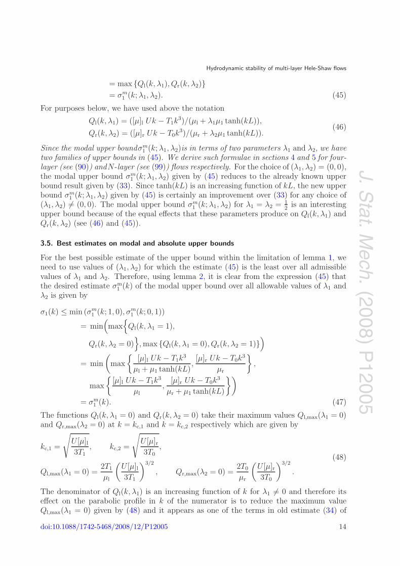
Figure 2. Four-layer fluid flow in a Hele-Shaw cell. The surface tensions at threeinterfaces are shown as T0, T1, and T2. The constant viscosities are increasing inthe direction of flow: μl < μ2 < μ1 < μr.

viscosity μl occupies an infinite region x < −2L and a fluid of viscosity μr > μl occupiesan infinite region x > 0. Two intermediate regions −L < x < 0 and −2L < x < −L havefluids of constant viscosities μ1 and μ2 respectively such that μl < μ2 < μ1 < μr. It isclear that there are three interfaces located at x = 0, −L, and −2L with correspondinginterfacial surface tensions denoted by T0, T1, and T2 respectively.

In this four-layer case, the relation (10) still holds away from all three interfaces andhence the relation (11) still holds in the exterior of the two internal layers of fluids withthe obvious modification:

f(x) = f(−2L) exp(k(x + 2L)), for x < −2L,

f(x) = f(0) exp(−kx), for x > 0.(80)

Then we have f−x (−2L) = kf(−2L) and f+

x (0) = −kf(0) in the exterior of theintermediate regions. The limit values of fx on the boundaries of the two internal layersare given by formulae similar to (38). Using these limit values at the interfaces in thelinearized dynamic and kinematic interfacial conditions, like in the three-layer case, aftersome algebraic manipulation, leads to the following three conditions at three interfaces,similar to (23):

−μ1(f−x f)(0) = (μr k − σ−1E0)f

2(0),

μ1(f+x f)(−L) − μ2(f

−x f)(−L) = −σ−1E1f

2(−L),

μ2(f+x f)(−2L) = (μl k − σ−1E2)f

2(−2L),

(81)

where

E0 = k2 U(μr − μ1) − k4T0,

E1 = k2 U(μ1 − μ2) − k4T1,

E2 = k2 U(μ2 − μl) − k4T2.

(82)

As before, we integrate equation (10) (which (9) reduces to in each layer) after multiplyingwith f(x) on the interval x ∈ (−2L, 0). In this interval, there is an interior interface atx = −L across which there is a jump in the values of μ and fx(x). Therefore, we split theintegral into two parts, namely on the intervals (−2L,−L) and (−L, 0). Thereby we get

−μ2

∫ −L

−2L

(fxf)x dx − μ1

∫ 0

−L

(fxf)x dx +

∫ 0

−2L

μf 2x dx + k2

∫ 0

−2L

μf 2 dx = 0. (83)

doi:10.1088/1742-5468/2008/12/P12005 20

J.Stat.M

ech.(2008)

P12005

Hydrodynamic stability of multi-layer Hele-Shaw flows

Upon integration and simplifying, we get

−μ2(f−x f)(−L) + μ2(f

+x f)(−2L) − μ1(f

−x f)(0)

+ μ1(f+x f)(−L) +

∫ 0

−2L

μ(f 2x + +k2f 2) dx = 0. (84)

Using (81) in (84) and then simplifying, the growth rate can be expressed as

σ2(k) =E0 f 2(0) + E1f

2(−L) + E2f2(−2L)

μrkf 2(0) +∫ 0

−2Lμ(f 2

x + k2f 2) dx + μlkf 2(−2L)

=E0f

2(0) + E1f2(−L) + E2f

2(−2L)

μrkf 2(0) + μ1 I1 + μ2 I2 + μl kf 2(−2L), (85)

where

I1 =

∫ 0

−L

(f 2x + k2f 2) dx, and I2 =

∫ −L

−2L

(f 2x + k2f 2) dx.

The subscript 2 on σ above refers to the four-layer case. We use lemma 1 for these twointegrals I1 and I2 in the above inequality. For each of these two integrals in lemma 1, weuse different pairs of constants (see lemma 1). Our convention below will be to use a pairof constants λ1,j and λ2,j for internal layer j defined as the layer in −jL < x < −(j−1)L.Thus for integral I1 which is over layer 1 (the rightmost internal layer), we use λ1,1 andλ2,1 in place of λ1 and λ2 respectively in lemma 1 (also see section 3.3). And similarly forother layers. Applying the lemma in this way, we obtain

μ1I1 + μ2I2 ≥ μ1{λ1,1f2(−L) + λ2,1f

2(0)}k tanh(kL)

+ μ2

{λ1,2f

2(−2L) + λ2,2f2(−L)

}k tanh(kL). (86)

The above two inequalities give us

σ2(k) ≤ E0f2(0) + E1f

2(−L) + E2f2(−2L)

F0f 2(0) + F1f 2(−L) + F2f 2(−2L), (87)

where the Ei are defined in (82) and the Fi are defined as follows:

F0 = k {μ1λ2,1 tanh(kL) + μr} ,

F1 = k (μ1λ1,1 + μ2λ2,2) tanh(kL),

F2 = k {μl + μ2λ1,2 tanh(kL)} .

(88)

We are interested in the modal upper bounds on the growth rates of all waves. For reasonsmentioned earlier in section 3.1, it is sufficient to analyze (87) for the upper bound whenall Ei > 0, i = 0, 1, 2, in (87), i.e., when wavenumber k is in the range

k2 ≤ min

{U(μ2 − μl)

T2

,U(μ1 − μ2)

T1

,U(μr − μ1)

T0

}. (89)

doi:10.1088/1742-5468/2008/12/P12005 21

J.Stat.M

ech.(2008)

P12005

Hydrodynamic stability of multi-layer Hele-Shaw flows

Therefore we apply inequality (32) (for k in the range given by (89)) to (87) and obtainthe following estimate of the upper bound on the growth rates of all waves:

σ2(k) ≤ max

{E0

F0

,E1

F1

,E2

F2

}

= maxλ1,j+λ2,j=1

{(μ2 − μl) Uk − T2k

3

μl + λ1,2μ2 tanh(kL),

(μ1 − μ2) Uk − T1 k3

(μlλ1,1 + μ2λ2,2) tanh(kL),

(μr − μ1) Uk − T0k3

μr + λ2,1μ1 tanh(kL)

}

= σm2 (k; λ1,1, λ2,1, λ1,2, λ2,2) ≡ σm

2 (k; λi,j). (90)

The procedure that we outlined in section 3 after (46) can be used to derive estimatesanalogous to (47) and (49). Since this is straightforward, we omit this here.

4.1. Upper bounds based on asymptotics

It is difficult to obtain an absolute upper bound from (90) over the entire spectrum ofwavenumbers for arbitrary values of the λ parameters within the constraint of lemma 1.However, for short waves and long waves, the asymptotic approximations to modal upperbound (90) are useful for the purposes of stability enhancement as before.

For kL � 1, the upper bound (90) can be approximated as

σ2,l(k) ≤ max

{kU(μ2 − μl)

μl + λ1,2kLμ2

,U(μ1 − μ2)

L(λ2,2μ2 + λ1,1μ1),

kU(μr − μ1)

μr + λ2,1kLμ1

}

= σm2,l(k; λi,j). (91)

The second term in the above expression does not depend on k. Therefore, the modalupper bound (91) is not arbitrarily small for long waves, i.e., when k tends to zero.Compare this with modal upper bounds σst(k) (see (1)) for the two-layer case and σm

1,l(k)(see (54)) for the three-layer case. This shows that the stability of long waves maynot always be enhanced in going from two- or three-layer flows to the four-layer flowsconsidered here.

For short waves kL ≥ 1, we have from (90)

σ2,s(k) ≤ max

{(μ2 − μl) Uk − T2k

3

μ2l

,(μ1 − μ2) Uk − T1 k3

μ12

,(μr − μ1) Uk − T0k

3

μr1

}

= σm2,s(k; λi,j), (92)

where c ≤ tanh(k∗L) and

μr1 = (μr + λ2,1μ1 c), μ12 = (λ1,1μ1 + λ2,2μ2)c, μ2l = (μl + λ1,2μ2 c). (93)

The subscript s in (92) refers to the ‘short’ wave regime as before. The terms in thesemodal upper bounds are similar in form to the formula (1) for the exact growth rate inthe two-layer case. An absolute upper bound (i.e., independent of k but dependent onthe parameters λi,j), denoted by σu

2,s(λi,j) and defined by σu2,s(λi,j) = max

k{σm

2,s(k; λi,j)} for

doi:10.1088/1742-5468/2008/12/P12005 22

J.Stat.M

ech.(2008)

P12005

Hydrodynamic stability of multi-layer Hele-Shaw flows

waves in this short wave regime, is then given by

σ2,s(k) ≤ max

{2T0

μr1

(U [μ]03T0

)3/2

,2T1

μ12

(U [μ]13T1

)3/2

,2T2

μ2l

(U [μ]23T2

)3/2}

= σu2,s(λi,j), (94)

where λi,j can take values within the constraint of lemma 1.

4.2. Sufficient conditions for stability enhancement

Improvement in stability for such four-layer flows over the two-layer case requires thatthe upper bound on the growth rate given by (94) be less than σst (see (2)). Using aprocedure described in section 3.6.3, we obtain the following formula analogous to (73) ofsection 3.6.3:

i=2∑i=0

αi

(Ti

T

)1/3 (μi,i+1

μl + μr

)2/3

> 1 +(μ2 − μ1)

(μr − μl), (95)

where μ0,1 = μr1 and μ2,3 = μ2l as defined above in (93). Above, α0 = 1, α1 = 2, α2 = 1.

5. Multi-layer flows

Consider N intermediate regions of equal length L in the interval (−NL, 0) in therectilinear Hele-Shaw cell of infinite length. Each of these regions contains constantviscosity fluids with fluid of viscosity μl occupying the leftmost infinite region x < −NLand fluid of viscosity μr occupying the rightmost infinite region x > 0. In the region(−pL,−pL + L), with p = 1, 2, . . . , N , the viscosity of the fluid is μp such thatμl = μN+1 < μN < μN−1 < · · · < μp < μp+1 < · · · < μ1 < μ0 = μr. We have(N + 1) number of interfaces located at xi = −iL, i = 0, 1, 2 . . . , N , and labeled as theith interface. For i = 0, 1, . . . , N , we denote the surface tension coefficient on the ithinterface at x = xi as Ti. Similarly, we use [μ]i = μi − μi+1 for the viscosity jump atthe ith interface, i = 0, 1, . . . , N . The flow, as before, in the cell is in the direction ofincreasing viscosity. Recall the previous section. A quite similar procedure and lemma 1give the following estimate:

σN ≤∑N

i=0 Ei f2(xi)∑N

i=0 Fi f 2(xi), (96)

where Ei = k2U [μ]i − k4 Ti, i = 0, 1, . . . , N , and the Fi are defined as follows:

F0 = k (μ1λ2,1 tanh(kL) + μr) ,

Fi = k (μiλ1,i + μi+1λ2,i+1) tanh(kL), i = 1, . . . , (N − 1),

FN = k (μl + μNλ1,N tanh(kL)) ,

(97)

with λ1,i ≥ 0, λ2,i ≥ 0 such that λ1,i + λ2,i ≤ 1, ∀ i = 1, . . . , N . For reasonsmentioned earlier in section 3.1, it is sufficient to analyze (96) for the upper bound for allEi > 0, i = 0, . . . , N , in (96), i.e., when wavenumber k is in the range given by

k2 ≤ mini

{U(μi − μi+1)

Ti

}, i = 0, 1, . . . , N. (98)

doi:10.1088/1742-5468/2008/12/P12005 23

J.Stat.M

ech.(2008)

P12005

Hydrodynamic stability of multi-layer Hele-Shaw flows

Applying the inequality (32) to the above formula (96) for waves in the range given by (98),we obtain the following estimate of the modal upper bounds on the growth rates of allwaves:

σN (k) ≤ maxλ1,i+λ2,i=1

{E0

F0,E1

F1, . . . ,

Ei

Fi, . . . ,

EN−1

FN−1,EN

FN

}

≤ maxλ1,i+λ2,i=1

{Q0, Q1, . . . , Qi, . . . , QN−1, QN}

= σmN (k; λi,j), (99)

where

Q0 =E0

F0=

kU [μ]0 − k3 T0

(μr + λ2,1μ1 tanh(kL)),

Qi =Ei

Fi=

kU [μ]i − k3 Ti

(λ1,iμi + λ2,i+1μi+1) tanh(kL), i = 1, . . . , (N − 1),

QN =EN

FN

=kU [μ]N − k3 TN

(μl + λ1,NμN tanh(kL)).

(100)

Following the procedure outlined in section 3 after (46), one can judiciously choosethe parameters λi,j for the best modal upper bound σm

N (k), analogous to (47), and forthe best absolute upper bound σu

N , analogous to (49). The absolute upper bound arisingfrom (99) will depend on parameters λ1,j and λ2,j, j = 1, . . . , N . In this parameterspace, this estimate is better with (λ1,j, λ2,j) �= (0, 0) even for some j ∈ [1, N ] than withλ1,j = λ2,j = 0, ∀ j = 1, . . . , N . The best estimate of this absolute upper bound σu

N

can be derived from (99) by the procedure outlined for the four-layer case in the previoussection. In fact, it is easy to see that a similar procedure will give an expression for σu

N

similar in form to (94) except that there will be N + 1 terms in its expression instead ofthree (see (94)). Since all this is straightforward along the lines of three-layer case treatedearlier, we omit any further details here.

5.1. Sufficient conditions for stability enhancement

Using a procedure similar to those used for other cases (see section 3.6.3), we obtain thefollowing generalization of the sufficient condition (95) from the four-layer case to this(N + 2)-layer case:

i=N∑i=0

αi

(Ti

T

)1/3 (μi,i+1

μl + μr

)2/3

> 1 +(μN − μ1)

(μr − μl), (101)

where α0 = 1, αN = 1, αi = 2, for i = 2, . . . , (N − 1), and

μ0,1 ≡ μr1 = μr + λ2,1μ1 c,

μi,i+1 = (λ1,iμi + λ2,i+1μi+1)c, i = 1, 2, . . . , (N − 1),

μN,N+1

≡ μNl

= μl + λ1,N

μN

c.

(102)

doi:10.1088/1742-5468/2008/12/P12005 24

J.Stat.M

ech.(2008)

P12005

Hydrodynamic stability of multi-layer Hele-Shaw flows

5.2. Upper bounds based on asymptotics

For long waves (i.e. kL � 1), using (96), (97), (99), and tanh(kL) ∼ kL, we obtain themodal upper bound σm

N,l(k; λi,j) for the individual wave with wavenumber k:

σN,l(k) ≤ σmN,l(k; λi,j) = max

{Ql

0, . . . , Qlp, . . . , Q

lN

}, (103)

where

QlN =

kU(μN − μl)

μl + μNλ1,NkL, Ql

0 =kU(μr − μ1)

μr + μ1λ2,1kL,

Qlp =

U(μp − μp+1)

(μpλ1,p + μp+1λ2,p+1)L, p = 1, . . . , (N − 1).

(104)

For short waves with kL ≥ 1, using (96), (97), and (99), we obtain an upper boundσu

N,s(λi,j) on the growth rate of waves in this short wave range:

σN,s(k) ≤ σuN,s(λi,j) = max

{Qs

0, . . . , Qsp, . . . , Q

sN

}, (105)

where

Qs0 =

2T0

μr + λ2,1cμ1

(U(μr − μ1)

3T0

)3/2

, QsN =

2TN

μl + λ1,NcμN

(U(μN − μl)

3TN

)3/2

,

Qsp =

2Tp

(λ1,pμp + λ2,p+1μp+1)c

(U(μp − μp+1)

3Tp

)3/2

, p = 1, 2, . . . , (N − 1).

(106)

5.3. Determination of the number of layers from the prescribed arbitrary growth rate ofinstability

In this section, we want to show that one can estimate the number of internal layers(N) that will ensure that the growth rate does not exceed a prescribed value, howeversmall, when the viscosity jumps across all layers are equal. In this case, μi − μi+1 =(μr − μl)/(N + 1). Therefore all viscosity jumps are equal. Moreover, we chooseλi,p = 1/2, ∀ i, p, for our estimations below. We estimate the above for short and longwaves separately.

First, we estimate for long waves. It then follows from (104), after using the fact thatka/(b + kc) < a/c for positive k, a, b, c, that

Ql0 < Q∗, Ql

N < Q∗, Qlp < Q∗/2, where Q∗ =

2U(μr − μl)

(N + 1)Lμl, (107)

and hence from (103),

σN,l(k) ≤ Q∗ =2U(μr − μl)

(N + 1)Lμl

.

From this, we see that the number of layers can be determined a priori from the desiredgrowth rate for long waves which can be as small as we please. For the growth rate notto exceed ε, this gives

(N + 1) >2U(μr − μl)

ε L μl

. (108)

doi:10.1088/1742-5468/2008/12/P12005 25

J.Stat.M

ech.(2008)

P12005

Hydrodynamic stability of multi-layer Hele-Shaw flows

Now for short waves, we use the estimate (106). Using the conditions μi > μl, (λ1,i +λ2,i)c ≤ 1, ∀ i = 1, . . . , N , in (106), we obtain from (105)

σN,s ≤2Tmin

μl c

(U(μr − μl)

3(N + 1)Tmin

)3/2

. (109)

Therefore, to obtain a growth rate less than ε, however small, we get the following estimatefor the number of layers of fluid:

(N + 1) ≥(

2

εμl c√

Tmin

)2/3 (U(μr − μl)

3

), (110)

where Tmin = min{T0, T − 1, . . . , TN}. Finally, using the above results (108) and (110),we get

(N + 1) > max

{2U(μr − μl)

ε L μl,

41/3U(μr − μl)

3(εμl c)2/3(Tmin)1/3

}, (111)

which gives the number of layers required for σ ≤ ε. Therefore, we can obtain a maximalgrowth rate as small as we please by increasing the number N of internal layers. Therefore,the two-layer Saffman–Taylor interfacial instability σst can be reduced by any factordesired simply by increasing the number of layers according to the relation (111). Thenumber of layers according to (111) is likely to be so high (due to the small value of ε)that sufficient condition (101) will be automatically satisfied.

Part II: Variable viscosity fluid layers

We consider three- and four-layer flows below each layer having a smooth viscous profilewith μx > 0 in each layer. Below, we first review three-layer flows from [9] very brieflyto recall the procedure in this variable viscosity case and to highlight the significance ofthe result. The procedure outlined will then be helpful in explaining the mathematicaldifficulty in obtaining similar results for the case of more than three layers in general.Moreover, the procedure provides a way for us to obtain some interesting results for thefour-layer case as we will shortly see.

6. Three-layer flows

The three-layer case (see figure 3) is briefly reviewed here from [9] for reasons cited above.Multiplying (9) by f(x) and then integrating on the interval (−L, 0), we obtain

(μ+f+x f)(−L) − (μ−f−

x f)(0) +

∫ 0

−L

μ(f 2x + k2 f 2) dx = σ−1k2U

∫ 0

−L

μxf2 dx. (112)

We recall the notation (f1f2)(x) = f1(x)f2(x) used before. Using boundary condition (21)in (112) and then simplifying leads to

σ =E1 f 2(−L) + E0 f 2(0) + k2 U

∫ 0

−Lμxf

2 dx

μl k f 2(−L) + μr k f 2(0) +∫ 0

−Lμ (f 2

x + k2 f 2) dx. (113)

Note that all terms in the denominator of (113) are positive. As in earlier sections,it is sufficient to analyze (113) for the upper bound when Ei > 0, i = 0, 1, i.e., when

doi:10.1088/1742-5468/2008/12/P12005 26

J.Stat.M

ech.(2008)

P12005

Hydrodynamic stability of multi-layer Hele-Shaw flows

Figure 3. Three-layer fluid flow in a Hele-Shaw cell. The surface tensions at twointerfaces are shown as T0 and T1. The middle layer has variable viscosity. Theflow is potentially unstable.

wavenumber k is in the range

k2 < min

{U [μ]rT0

,U [μ]lT1

}, (114)

where [μ]r = (μr − μ−(0)), and [μ]l = (μ+(−L) − μl). As before, applying theinequalities (32)–(113) for k in the range given by (114) (so that E1 and E2 are positive),

we obtain after neglecting the positive term∫ 0

−Lμ f 2

x in the denominator of (113) thefollowing estimate of the upper bound on the growth rates of all non-trivial waves:

σ < max

{E1

kμl,

E0

kμr,

U

μlsup

x{μx}

}

= max

{[μ]r Uk − T0k

3

μr

,[μ]l Uk − T1 k3

μl

,U

μl

supx{μx}

}. (115)

The absolute upper bound (i.e., the growth rate of any unstable wave cannot exceed thisbound) is then given by

σ < max

{2T0

μr

(U [μ]r3T0

)3/2

,2T1

μl

(U [μ]l3T1

)3/2

,U

μlsup

x{μx}

}. (116)

For the ‘optimal’ viscosity profile given by

supx

(μx) ≤μl

Umax

{2T0

μr

(U [μ]r3T0

)3/2

,2T1

μl

(U [μ]l3T1

)3/2}

, (117)

doi:10.1088/1742-5468/2008/12/P12005 27

J.Stat.M

ech.(2008)

P12005

Hydrodynamic stability of multi-layer Hele-Shaw flows

the estimate (115) becomes

σ < max

{2T0

μr

(U [μ]r3T0

)3/2

,2T1

μl

(U [μ]l3T1

)3/2}

. (118)

Note the significance of this result: if the limit viscosities μ+(−L) and μ−(0) atthe two interfaces are close enough to μl and μr respectively and if we use the optimalprofile (117) for the middle layer, then the upper bound on the growth rate becomesarbitrarily small and the flow is almost stable. However, to generate the optimal profileon the basis of this upper bound, length L of the middle layer can, in principle, be verylarge since the gradient of the viscosity at any point in the interior layer cannot exceeda predetermined small value which is dependent on the growth rate itself and (μl/U)according to relation (117).

We see from (113) that μx > 0 for the middle layer has a destabilizing effect and μx < 0has a stabilizing effect. This also holds in the two-layer case with the middle-layer profileextending all the way up to −∞ because in this case the first terms from the numeratorand the denominator of (113) drop out. Such viscous profiles are automatically createdwhen a shear thinning or shear thickening fluid is used as a displacing fluid. Therefore,if we just use this non-Newtonian property of these complex fluids within the Newtonianframework of this paper, then we expect similar kinds of stabilizations and destabilizationsof instabilities when such fluids are used as displacing fluids. In fact, recent works onviscous fingering in complex fluids [16]–[21] show this to be the case even in the highlynon-linear regime of viscous fingering. Therefore, in the absence of understanding based onexact non-linear theory of non-Newtonian complex fluids, we believe that our results andapproach presented in this paper may be useful in interpreting some of the experimentalresults on viscous fingering in complex fluids.

7. Four-layer flows

The physical set-up here is same as in the constant viscosity case addressed in section 4except that each of the two internal fluid layers has a smooth viscous profile μ(x) withμx > 0. This flow has three interfaces, one at x = 0 with surface tension T0, and anothertwo at x = −L,−2L with surface tensions T1, T2 respectively. We assume that each ofthe two extreme interfaces at x = −2L and 0 has positive viscosity jump in the directionof flow. The middle interface at x = −L can have a similar positive viscosity jump in thedirection of flow but, as we will see below, some interesting results can be obtained whenthe viscosity jump at this middle interface in the direction of flow is negative.

The mathematical problem is still defined by equation (9) in each layer, though thisequation simplifies to (10) in the exterior layers: x < −2L, x > 0, Because of this, far-field behavior defined by (80) still holds, because of which f−

x (−2L) = kf(−2L) andf+

x (0) = −kf(0) on the exterior side of the outer two interfaces. The limit values of fx onthe boundaries of the two internal layers are given by formulae similar to (38). Using theselimit values at the interfaces in the linearized dynamic and kinematic interfacial conditions,like in the four-layer constant viscosity case of section 4, after some algebraic manipulation,leads to the following three interfacial boundary conditions at x = −2L, x = −L, x = 0,

doi:10.1088/1742-5468/2008/12/P12005 28

J.Stat.M

ech.(2008)

P12005

Hydrodynamic stability of multi-layer Hele-Shaw flows

similar to (81):

−(μ−f−x f)(0) = μr kf 2(0) − σ−1E0 f 2(0),

(μ+f+x f)(−L) − (μ−f−

x f)(−L) = −σ−1E1 f 2(−L),

(μ+f+x f)(−2L) = μl kf 2(−2L) − σ−1E2 f 2(−2L),

(119)

where

E0 = E0(k) = k2U [μr − μ−(0)] − k4T0,

E1 = E1(k) = k2U [μ+(−L) − μ−(−L)] − k4T1,

E2 = E2(k) = k2U [μ+(−2L) − μl] − k4T2.

(120)

In contrast with the constant viscosity case in section 4 where equation (10) wasintegrated, now equation (9) is integrated on the interval x ∈ (−2L, 0) after multiplyingwith f as in the previous section. In this interval, μ(x)fx(x) is discontinuous at the interiorinterface location x = −L. Therefore the integral is split into two parts, namely on theintervals (−2L,−L) and (−L, 0). Thus we get

−(μ−f−x f)(−L) + (μ+f+

x f)(−2L) − (μ−f−x f)(0) + (μ+f+

x f)(−L) +

∫ 0

−2L

μf 2x dx

+ k2

∫ 0

−2L

μ f 2 dx = σ−1k2U

∫ 0

−2L

μxf2 dx. (121)

Using relations (119) in (121) and then simplifying we obtain

σ =E2f

2(−2L) + E1f2(−L) + E0f

2(0) + k2∫ 0

−2Lμx f 2

μl kf 2(−2L) + μr kf 2(0) +∫ 0

−2Lμ(f 2

x + k2f 2) dx. (122)

We see that the numerator of (122) contains f 2(−L) which does not appear in thedenominator. Because of this, for positive viscosity jump in the direction of basic flowat each of the three interfaces (when E0, E1, E2 > 0 for waves in the range given earlierin (89)) (122) cannot be reduced to a form to which the inequality (32) can be appliedas we have done in previous cases to obtain an estimate of the upper bound in termsof the parameters of the problem. We can do so only if we allow the viscosity jump(μ+(−L)−μ−(−L)) at the interior interface at x = −L to be negative, instead of positive,in the direction of basic flow. Then E1 < 0 for waves in the range (89) and the terminvolving f 2(−L) in the numerator of (122) is negative. Therefore, separating E1 fromthe numerator recasts (122) as the difference between the ‘first part’ and the ‘second part’where the ‘first part’ is a ratio similar in form to (113) and the ‘second part’ is a positivequantity proportional to (μ−(−L) − μ+(−L)). A consequence of this observation is thatan absolute upper bound similar to (116) is obtained by neglecting the ‘second part’,namely

σ < max

{2T0

μr

(U [μ]r3T0

)3/2

,2T2

μl

(U [μ]l3T2

)3/2

,U

μl

supx{μx |x �= −L,−2L, 0}

}. (123)

We see that this absolute upper bound for the optimal profile (117) will be arbitrarilysmall if positive viscosity jumps at the x = −2L and 0 interfaces in the direction of

doi:10.1088/1742-5468/2008/12/P12005 29

J.Stat.M

ech.(2008)

P12005

Hydrodynamic stability of multi-layer Hele-Shaw flows

Figure 4. Four-layer fluid flow in a Hele-Shaw cell. The two internal layers havevariable viscosity and thus each of these layers is potentially unstable individually.The two extreme interfaces are also unstable individually except for the internalinterface. This multi-layer flow could be overall potentially stable if the internalinterface is strongly stable on its own.

flow are small enough for reasons given after (117). Therefore, the maximum growthrate will be less than this absolute upper bound by a positive amount proportional toμ−(−L)−μ+(−L) > 0. If (μ−(−L)−μ+(−L)) > 0 is large enough, the maximum growthrate could be negative and the flow could be stable. Thus, in spite of the fact that internallayers and outer interfaces are individually unstable, this four-layer flow overall is stableonly due to the middle interface being strongly stable on its own. Such a potentiallystable configuration is shown in figure 4; keep in mind that the jumps in viscosities arenot shown on a true scale.

Part III: Discussion and concluding remarks

8. Conclusions

In this paper, we have obtained the following results.

(1) For three-layer Hele-Shaw flows with constant viscosity layers, a new absolute upperbound (53) on the growth rate of instabilities is obtained as a non-strict inequality.Thus, this bound can in principle be reached for a non-trivial disturbance. This isa considerable improvement over the absolute upper bound (34) which could not bereached for a non-trivial disturbance. A potential application of this is to controlthe instability of an interface separating low viscosity fluid from a high viscosity fluidthat it is displacing. The way to do this is to introduce an intermediate layer of fluidwith properties that will satisfy the two-parameter family of sufficient conditions (76)for enhancement of stability. The condition (77) is interesting because it does notdepend on the viscosity μ ∈ (μl, μr) of the fluid in the middle layer. These results areof significance for the design of effective enhanced oil recovery methods.

(2) We extended the above results to four-layer flows (see section 4), all layers havingconstant but different viscosity fluids. This four-layer case is important in setting thestage for a generalization to arbitrary number of layers of constant viscosity fluids andin exemplifying the difficulties associated with deriving similar results when internallayers have potentially unstable viscous profiles.

(3) In section 5, the above mentioned results were generalized to arbitrary number oflayers. As an application of these results, we have shown that the instability of

doi:10.1088/1742-5468/2008/12/P12005 30

J.Stat.M

ech.(2008)P

12005

Hydrodynamic stability of multi-layer Hele-Shaw flows

potentially unstable two-layer or three-layer flows with constant viscosity fluid layerscan be significantly reduced to any desired level, however small, by increasing thenumber of layers (see section 5.3).

(4) An absolute upper bound result for the three-layer case with potentially unstablemiddle layer is revisited. It is shown that extension of this to the four-layer casewhen both the internal layers and the three interfaces are individually unstable runsinto difficulty with our approach. Thus this is an open problem. However, in thisfour-layer set-up, an absolute upper bound is obtained using our approach providedthe middle interface is individually stable (meaning that the viscosity jump is negativein the direction of flow at this interface). In fact, we have shown that if this viscosityjump at the middle interface is large enough, the upper bound on the growth ratecould in fact be negative and the flow overall could be stable.

Within the framework of the results itemized above, if one is to devise ways tosignificantly stabilize a viscosity jump driven unstable two-layer flow, there are threealternatives:

(i) use of successive constant viscosity fluid layers with appropriate interfacial surfacetensions so that sufficient conditions for stability enhancements are satisfied;

(ii) use of a fluid layer in between whose viscous profile is optimal, given by (117), andwhere the limit viscosities μ+(−L) and μ−(0) at the two interfaces are close enoughto μl and μr respectively;

(iii) use of two internal fluid layers with viscous profiles of the internal layers such thatthe middle interface is strongly stable.

Towards this end, we must stress that many of the results obtained in this paperare general in character and that the techniques used hold promise for applications toother unstable multi-layer flows such as Rayleigh–Taylor unstable flows, coating flows, jetflows, and Kelvin–Helmholtz flow, to mention but a few. These results are obviously offundamental and practical importance to many applications where stability of flows playsa decisive role. One instance of such an application is that of enhanced oil recovery bypolymer flooding [5]–[7].

Acknowledgment

The author is grateful to two reviewers for their constructive criticisms which have helpedus to improve the paper.

References

[1] Hele-Shaw H S, On the motion of a viscous fluid between two parallel plates, 1898 Trans R. Inst. Na. Archit.Lond. 40 218

[2] Darcy H, 1856 Les Fontaines Publiques de la Ville de Dijon Victor Dalmond[3] Saffman P G and Taylor G I, The penetration of a fluid in a porous medium or Hele-Shaw cell containing a

more viscous fluid , 1958 Proc. R. Soc. A 245 312[4] Drazin P G and Reid W H, 1981 Hydrodynamic Stability (London: Cambridge University Press)[5] Slobod R L and Lestz J S, Use of a graded viscosity zone to reduce fingering in miscible phase

displacements, 1960 Producers Month. 24 12[6] Uzoigwe A C, Scanlon F C and Jewett R L, Improvement in polymer flooding: the programmed slug and the

polymer-conserving agent , 1974 J. Petrol. Tech. 26 33–41

doi:10.1088/1742-5468/2008/12/P12005 31

J.Stat.M

ech.(2008)

P12005

Hydrodynamic stability of multi-layer Hele-Shaw flows

[7] Shah D and Schecter R, 1977 Improved Oil Recovery by Surfactants and Polymer Flooding(New York: Academic)

[8] Daripa P and Pasa G, On the growth rate for three-layer Hele-Shaw flows: variable and constant viscositycases, 2005 Int. J. Eng. Sci. 43 877

[9] Daripa P and Pasa G, A simple derivation of an upper bound in the presence of viscosity gradient inthree-layer Hele-Shaw flows, 2006 J. Stat. Mech. P01014

[10] Daripa P, Studies on stability of three-layer Hele-Shaw flows, 2008 Phys. Fluids 20 112101[11] Daripa P and Pasa G, New bounds for stabilizing Hele-Shaw flows, 2004 Appl. Math. Lett. 18 1293[12] Gorell S B and Homsy G M, A theory of the optimal policy of oil recovery by the secondary displacement

process, 1983 SIAM J. Appl. Math. 43 79[13] Saffman P G, Viscous fingering in Hele-Shaw cells, 1986 J. Fluid Mech. 173 73[14] Howison S D, Complex variable methods in Hele-Shaw moving boundary problems, 1992 Eur. J. Appl. Math.

3 209[15] Daripa P and Pasa G, An optimal viscosity profile in enhanced oil recovery by polymer flooding , 2005 Int. J.

Eng. Sci. 42 2029[16] Ben Amar M and Poire E C, Pushing a non-Newtonian fluid in a Hele-Shaw cell: from fingers to needles,

1999 Phys. Fluids 11 1757[17] Chevalier C, Ben Amar M, Bonn D and Lindner A, Inertial effects on Saffman–Taylor viscous fingering ,

2006 J. Fluid Mech. 552 83[18] Lindner A, Bonn D, Poire E C, Ben Amar M and Meunier J, Viscous fingering in non-Newtonian fluids,

2002 J. Fluid Mech. 469 237[19] Lindner A, Coussot P and Bonn D, Viscous fingering in a yield stress fluid , 2000 Phys. Rev. Lett. 85 314[20] Lindner A, Bonn D and Meunier J, Viscous fingering in a shear-thinning fluid , 2000 Phys. Fluids 12 256[21] Lindner A, Bonn D and Meunier J, Viscous fingering in complex fluids, 2000 J. Phys.: Condens. Matter

12 A477

doi:10.1088/1742-5468/2008/12/P12005 32