ll2 Transportation Research Record 1034

J- Integral and Cyclic Plasticity Approach to Fatigue and Fracture of Asphaltic Mixtures

A. A. ABDULSHAFI and KAMRAN MAJIDZADEH

ABSTRACT

A nationwide survey of pavement performance indicated that fatigue is the most important distress problem in U.S. primary pavements. The classical approaches to investigating fatigue problems are classified as phenomenological and mecha­nistic. The phenomenological approach is based on developing a distress func­tion using laboratory simulation of third-point beam loading, beam on elastic foundation, discs, and so fm:th; its main drawback is that most of the fatigue life is exhausted through cyclic plasticity, and crack initiation, propagation, and ultimate failure, with the associated stress and strain redistributions, are not accounted for. The mechanistic approach is based on the laws of linear elastic fracture mechanics (LEFM) to model laboratory-simulated ci:ack initi­ation, propagation, and unstable failure; its main shortcoming is that failure is assumed to be by brittle fracture and the initiation phase is not modeled becam~e lt lo; ao;o;umeu that " c:rack. size of "c0 " inilially exists. Moreover, the stress intensity factor requires rather specialized computational tech­niques like finite elements. In this paper, a cyclic plasticity fatigue model is developed through laboratory-controlled stroke fatigue testing of unnotched disc samples of asphaltic mixes. This model is statistically matched with con­trolled stroke fatigue testing of notched discs under the same stroke range loading condition. Another model is developed for fatigue crack propagation using the elasto-plastic fracture mechanics (EPFM) approach. The EPFM fracture criterion is the path-independent contour J-integral. Within the development of the propagation model, a method for J-integral testing of asphal tic mixtures has been established. An example is presented and worked out to illustrate how this new approach can be used in modeling fatigue life.

A nationwide survey of pavement performance (1) in­dicated that fatigue of primary pavements is gen­erally the most important distress type. Fatigue is defined as "the phenomenon of fracture under re­peated or fluctuating stress having a maximum value much less than the tensile strength of the material" (2). In connection with this definition, a failure criterion has to be defined. Failure is a complex process that is based on the damage accumulation concept. An introduction to the mechanisms by which damage progresses in the continuum under load appli­cations is instructive in casting light on the fail­ure manifestations.

Damage can be defined as a structure-sensitive property that is imparted to the material through the influence of defects (microscopic or macroscopic cracks, voids, dislocations, and oo forth) that are naturally or artificially introduced, thereby ren­dering the material inhomogeneous (3). The progres­s ion of damage under load applications is due to internal irregularities or defects that grow grad­ually to a certain critical size; thereafter, growth is unstable. In engineering materials, damage has been categorized by two different conditions: duc­tile (plastic flow) or brittle (elastic fracture). This implies that fatigue is not, in itself, a sin­gle physical phenomenon but rather a condition brought about by several different processes that may lead to the disintegration of a body by the ac­tion of mechanical forces <i>· Damage may therefore progress within a material under the different mech­anisms of fracture and flow, depending on critical values of stresses, strains, and environmental and temperature conditions. A material may have more

than one character is tic parameter to be evaluated when different damage mechanisms operate at critical levels.

It can be postulated that cracks (not voids that are considered probabilistic crack initiators) and plastic deformation (which may be accompanied by viscous flow) are valid material failure criteria. Observations of the type of failure occurring within a continuum can reveal which condition dominates during the damage process. However, in real-life materials, the state responsible for damage reverses randomly, making fracture and plastic deformation equally probable. The distribution and progression of damage are random processes that are spatial, time dependent, and temporal. Whether or not a con­tinuum exhibits fracture or inelastic flow depends on many factors, including the normal stresses, the tensile or shear stress required to cause fracture, the shear stresses, the shear stress required for inelastic flow, and moisture and temperature con­ditions.

CLASSICAL APPROACHES TO FATIGUE PROBLEMS

Approaches to the fatigue problem can be classified as phenomenological or mechanistic. In the first approach, laboratory testing of a beam or disc under controlled load (stress) or controlled stroke ( str.ain) loading mode is used to develop stress or strain versus number of cycles to failure (S-N) curves. Due to the scatter of results, a regression analysis is usually employed to fit the obtained

Abdulshafi and Majidzadeh

data and arrive at a mathematical expression (dis­tress function) such as that of Pell's equation (2_):

Nr = c (l/a or er (1)

where

Nf number of load applications to failure; £ = amplitude of applied tensile strain in con­

trolled strain mode; a = amplitude of applied stress in controlled

stress mode; and c,m = factors that depend on the material compo­

sition, mix properties, and loading mode.

Research has indicated (6) that controlled strain mode is appropriate for thin (2 in. or less) pave­ments and controlled stress mode is appropriate for thick stiff pavements (greater than 6 in.). Between these two ranges in thickness, some form of loading intermediate to both controlled strain and stress is appropriate. Investigations in the past 20 years have been concerned with effects of factors such as using trapezoidal-shaped cantilever beams (7-9), compound loadings (10) , frequency (11) , and -rest periods (12) on the distress function:-In short, it has been noted that although this approach gained universal acceptance, its limitation is that it can­not account for crack initiation and propagation and the subsequent redistribution of stresses within the layered system (13).

Mechanistic approaches using the application of fracture mechanics are based on nominal or local stress-strain analysis. It has been speculated that the major deficiencies in inaccurate prediction of fatigue life based on nominal stress analysis could be overcome if local stress-strain in the immediate vicinity of a stress raiser were considered instead.

The nominal stress-strain mechanistic approach developed at Ohio State University is credited to Majidzadeh et al. (14). This approach is based on the postulate that fatigue life can be described by the process of crack initiation, propagation, and ultimate fracture. These three damage ~ocesses in­clude material parameters that can characterize fa­tigue and fracture and that can be related as

Nr = </> (c0 , A, n, K, KIC)

such that

where

c0 = initial crack length, A,n material constants,

K =elastic stress intensity factor, and KIC elastic fracture toughness.

(2)

(3)

A and n are affected by such parameters as load frequency, external boundary conditions, tempera­ture, and statistical distributions of flaws in the materials as well as the dimensions of the models used. Extensions to Maj idzadeh' s work in applying linear elastic fracture mechanics (LEFM) include research studies on the effects of frequency (2_) ,

crack tip plasticity (15), and wave form and com­pound loading (16) On Crack propagation; however I

the idea of usin9""°LEFM remains the same. Laboratory experimentation to find the fracture­

fatigue function involves testing a beam on an elas­tic foundation and monitoring crack advance versus the number of load applications. The data thus ob­tained can be fitted by least squares approximation

113

procedures of regression analysis to arrive at a best fit. A two-term model fit can take the form:

implying that

Nf Cf f dN = f [dc/(a 1k 1 +a2 Ki)J 0 c0

Hence,

NEW CONCEPTS IN FATIGUE MODELING OF ASPHALTIC MIXTURES

Introduction

(4)

(5)

(6)

In a laboratory-controlled setting, given a valid constitutive law, it should be possible to predict laboratory sample performance, namely rutting and fatigue in asphaltic mixtures, with reasonable ac­curacy. Both laboratory and field investigation in­dicate that the failure of asphaltic mixes for a given set of loading conditions could be due to rut­ting (permanent deformation), fatigue cracking, or a combination of the two. Whether material parameters are stress or environment dependent, or both, is a subject of controversy.

The authors are inclined to believe that the material will exhibit a range of characteristic be­havior within which the material parameters are un­coupled from stress and environmental conditions. Further, examination of sample failures will reveal the states that dominate at the unstable failure conditions. That is where laboratory samples attain their importance as an indicator of field perfor­mance.

Following this point leads to another point of controversy--simulation of the fatigue problem. It has been argued that fatigue life determined from small laboratory specimens could be misleading in determining the fatigue life of an actual pavement (14,16); this is because it has been observed that mostof the fatigue life of a small, smooth, un­notched specimen will be consumed in initiating a crack and, therefore, the final stages of crack propagation and ultimate failure become indistin­guishable within the data scatter (16-18,p.132). The question of whether these are typicalof field ob­servations cannot be directly addressed; however, inconsistent correlations of fatigue life predicted from laboratory testing indicate that more research needs to be done.

To better simulate the failure conditions or de­termine where the importance of fracture toughness 1 ies, fracture conditions must be induced in the small specimens. To promote early crack growth, it is proposed that notched specimens be used, A model could then be developed to make a comparison between notched and unnotched specimens, and another model could be developed for crack growth.

In the analysis of unnotched specimens, cyclic plasticity and energy balance should be the tools by which the analysis is effected. On the other hand, the notched specimens should be investigated within the framework of lo<:al stress-strain analysis that will directly introduce the elasto-plastic (or time­dependent) fracture mechanics approach.

Exhaustion of Ductility Model (unnotched samples)

Fatigue life passes through three distinct periods: initiation of a crack, propagation of the crack to a

114

critical size, and ultimate failure. In each life period, there is a damaging mechanism or mechanisms that exhaust energy and lead to transition to the other phase. Many research studies have been done, especially in metallurgical engineering, postulating theories for the cause or causes of fatigue: how­ever, most of these theories conclude that inhibi­tion of fine slips that grow to a crack that will subsequently propagate and lead to ultimate failure is the cause of fatigue. Morrow (17) explained that, on the microscopic level, the cyclic plastic strain is related to the movement of dislocations, and the cyclic stress is related to the resistance to their motion. According to Morrow, repeated stress without accompanying plastic strain will not cause fatigue damage nor would repeated slip without repeated stress. He also suggested a tentative set of six fatigue fracture properties that are shown to apply well to SAE 4340 steel. These six fatigue properties will be examined to determine their applicability to asphalt fatigue models.

These properties are associated with coefficients that could be obtained from controlled stroke labo­ratory fatigue experimentation shown in Figure 1 as b, c, and £fr and from Sf and S. The mathematical representation of the suggested fatigue model is

(7)

The first four coefficients will be defined later, and Sf is the strength limit (associated with endurance limit) and S is the standard devia­tion of data scatter.

The controlled stroke fatigue coefficients shown in Figure 1 are defined as

I

Ef =

I

af

b

c =

fatigue ductility coefficient--the strain in­tercept of the ductility line at N • 1 cycle: it is related to Efr where •f = the mono­tonic fracture ductility: fatigue strength coefficient--the strain in­tercept of the strength line at N = 1 cycle divided by E: it is related to af, where af =the monotonic fracture strength: fatigue strength exponent--the slope of the strength line: and fatigue ductility exponent--the slope of the ductility line.

The idea of this scheme is to construct the fa­tigue curve without the need for doing "fatigue testing.• This can be done by evaluating the mono-

Transportation Research Record 1034

tonic coefficients (•f• af, and E) and using the uni­versal slopes b and c. The universal slopes are well established in the metallurgical engineering field: however, their applicability to asphaltic mixtures has not been researched until now.

The scheme of characterizing fatigue through six coefficients is advantageous in that the coeffi­cients relate to other engineering properties of as­phaltic mixtures that are routinely determined. The mathematical expressions for this model will be ref­erenced in a later section. This model applies to ductile failures where "cracking life is short" and used with a brittle failure model to predict crack initiation life.

The main criticism of the scheme is that field performance is not simulated by using small labora­tory samples that exhaust most of their fatigue life in the crack initiation phase. The model that repli­cates field conditions should contain crack propaga­tion and ultimate failure matched with the cyclic plasticity model. Matching criteria should be mod­eled by an expression for the actual number of cy­cles to initiate a crack. This will be addressed in a subsequent section of this paper.

Fracture Mechanics Considerations

Plastic zones created in the material when it is subjected to alternating low stress levels are mainly due to crack presence. In addition, during each loading cycle the sharp aggregate corners transmit point loading conditions to the asphalt cement with a stress singularity. Hence, even before crack formation, a plastic zone exists at each (sharp aggregate corner-asphalt cement) contact, and energy is dissipated through cyclic plasticity. Once a crack is initiated, then at the tip of the crack, stresses assume an inverse, square root stress (and strain) singularity. Because the material can toler­ate stresses up to its yield point, a plastic zone around the crack tip forms and blunts the crack ad­vance. The size of this plastic zone is critical in the analysis of fatigue life. If the formed plastic zone is small compared to the crack size and the geometry of the continuum, linear elastic fracture mechanics (LEFM) is approximating conditions of failure favorably (small scale yielding) • On the other hand, if the size of the plastic zone cannot be ignored (several orders of magnitude of the crack size), a nonlinear fracture mechanics approach is more appropriate.

Ef line

w

2 of ·.-1

'° Al -E-M

' .... curve

CJ) Fatigue strength line

with slope = b

LOG. Reversals to Failure, Nf

FIGURE 1 Controlled stroke fatigue diagram-fatigue coefficients.

Abdulshafi and Majidzadeh

In asphaltic mixtures, cracks usually develop at the bottom of the asphaltic layer due to tensile stresses exceeding a threshold yield stress value. This provides an opening mode fracture, designated as Mode 1. Further, the crack propagates vertically but in a zig-zag path, indicating either an aggre­gate obstruction or a weak contribution of Mode 2 loading type i however, for all practical purposes, Mode 1 can be considered dominating.

Hence, in the first case (LEFM), the material is assumed to exhibit brittle fracture (KI dominant region) where the Mode 1 critical stress intensity factor (KlC) is the material fracture characteristic. In the second case, the material is assumed to ex­hibit ductile fracture (J-dominant region) where JlC represents the material elasto-plastic fracture characteristics.

Bituminous mixtures can exhibit brittle or duc­tile fracture, depending on the state of stress at failure, which, in turn, depends on such factors as temperature, loading conditions, hardening or soft­ening induced, and inherent properties. Furthermore, the literature indicates that (19)

! E plane stress

E' = 1E/1 - v2 plane strain (8)

where

J1 s path-independent Mode 1 contour J-integral, K1 Mode 1 elastic stress intensity factor, E uniaxial elastic modulus, v = Poisson's ratio,

G1 strain energy release rate, 6t crack opening displacement, ay yield strength, and

y scalar multiplier.

At the incipient crack conditions, the fracture criterion is

K1 = KIC and JI =lie (9)

and the relationships given in Equation B hold. In fact, Begley and Landes (19) have used small,

fully plastic specimens to determine Jic values. These values were found to be in good agreement with Kic values obtained from large independent elastic specimens that satisfied plane strain fracture toughness requirements.

It is apparent then that Jic is an appropriate material characterization for both elastic and elasto-plastic fracture mechanics approaches. The exper !mental evaluation of J and J IC can be found elsewhere (20). The basic idea behind the develop­ment of a J-integral testing procedure is to inter­pret the J-integral as the energy release rate (.!!) : then,

J = (-1/B) (au/aa) It> It> means b. is held fixed

where

B specimen thickness, U total strain energy, a crack length, and ~ = load-point displacement.

(10)

For simplicity, elastic unloading is considered only at the fracture point for the monotonic load­ing, and U can be found as the area under the load­displacement curve. Development of the appropriate fracture mechanics models to describe the fatigue

115

life of asphaltic mixtures is considered in the next section.

Development of Fatig ue Fracture Models

Fatigue Crack Propagation Model (notched sample)

To promote crack propagation, a notch has to be in­troduced into the sample, together with a fine, sharp-edged crack, Manson (16) has suggested that

dc/dN =A" c

where

c = crack length, N number of cycles at crack length c, and A s material constant.

The LEFM considers

(I I)

(12)

The extension of the J-integral to the elastic case gives (from Equation B)

Substituting into Equation 12 gives

C = JE '/CT2=1/a ~E = J/2U0 (13)

where Ue is elastic strain energy and J is J(c,U) where U is the total strain energy.

Substitute Equation 13 into Equation 11 to get

dc/dN = A(J/2Ue) (I4)

Equation 14 represents the crack propagation model. Experimentally (20) (a) a J-c curve will be estab­lished, where Ue can also be found and (b) a c-N relationship will be found by performing fatigue tests on notched specimens. This relationship will be differentiated to obtain the (dc/dn) versus N relationship. Now, for certain N, c and dc/dN can be obtained. From (a) , J that corresponds to c can be obtained and then the relationship (dc/dN) - J can be established. The slope of this relationship should be A/2Ue.

Crack Initiation Model

Only a theoretical model is discussed in this sec­tion because crack initiation will be determined ex­per !mentally by monitoring the number of cycles to propagate different size cracks of the disc speci­mens. The theoretical discussion of the crack initi­ation models serves as an introduction to a fol­low-up paper.

From Equation 14,

dN = (2Ue/AJ) *de= dJ/(J *A) (15)

Therefore,

/ dN = / (dJ/J) * (1/A) (16) No Io

and therefore,

(I 7)

where J 0 and N0 correspond to the initial lower bound values of the J-integral and the number of cycles

ll6

below which the crack propagation law (Equation 11) does not hold.

rhe parameter A is assumed to be a material con­stant. To provide the appropriate condition for the assumption of parameter A, a loading condition should be set such that the size of the plastic zone ahead of the crack tip is constant and moving very slowly during propagation.

The upper limit of the validity of Equation 17 is when N tends toward Ney and J tends toward Jrci hence,

(18)

Substituting into Equation 17 gives

(19)

where Ccy and NC"(. are critical crack length and corresponding critical number of cycles at which the third phase of unstable failure commences.

Divide Equation 17 into Equation 19 to obtain

(20)

For Equation 20, J depends on assuming an ini­tial detectable crack size in which a definition ia required. The detectable length varies as a function of the measuring devices. Extremely short crack lengths are determined with extremely sensitive mea­suring devices like the scanning electron microscope and ultrasonic and acoustic emission. Alternatively, an "engineering size crack" that is detectable to the eye could be found experimentally as follows: N0 to propagate different crack sizes should be recorded and a re·lationship between N0 /J\:y and c es­tablished. This relationship could be extrapolated to find the era.ck size c~ at N/Nc::y " 0. ,

From the c-J relationship, the , value of c 0 is entered and the corresponding J 0 is obtained, This value should be substituted in Equation 20 in­stead of J0 , Now Equation 20 will reduce to the nondimeneional relationship,

J = f (t.N/l:INr) (21)

where N is the number of ,cycles required to propa­gate a crack from size c 0 to any arbitrary value c that corresponds to N.

Ultimate Failure Model

The ultimate failure model is defined by finding the number of cycles associated with unstable crack propagation. Unstable crack propagation occurs dur­ing the last cycles of fatigue life where the crack opens under extremely low loading conditions and, in this case, J " J IC' The number of cycles from the critical crack size (Ccyl until complete failure is monitored experimentally for each initial crack size and denoted as 6Nf •

A relationship between the dimensionless quantity c/D and 6Nf, where Dis the sample diameter, is es­tablished as a model for ultimate failure. The other alternative is to use the relationship between 6cf/D and 6Nf, where 6Cf is the remaining length at the on­set of unstable crack growth. The better correlated relationship will be used in this paper. In as­phaltic mixtures, however, the contribution of this phase to fatigue life is minimal.

Matching Model

At this point, a form of relationship to serve as a matching criterion between notched and unnotched

Transportation Research Record 1034

specimen test results should be established to enable the determination of the number of cycles required to initiate an engineering size crack cor­responding to C0 '. For this purpose, notched spec­imens should be subjected to the same stroke range loading conditions as the unnotched specimens, and the number of cycles required to initiate a detect­able-to-the-eye crack recorded as N0 '. A regression line between N0 ' from the notched specimens· and N from the unnotched specimens will establish the re­quired relationships.

Summary of the Proposed Fatigue Life Model

Fatigue life is then calculated according to the following formula:

where

Nf N ' 0

(6Nf)

(22)

total fatigue life, number of cycles to initiate a crack, c0 '; this is obtained (at present) from the matching model. number of cycles required to propagate a crack from c0 ' to Ccyl this is obtained from the crack propagation model. number of cycles required to open the crack from Cc to ultimate failure; this is obtained from the ultimate failure model.

The simple procedure for determining these terms is as follows:

1, Establish cyflic plasticity fatigue curve us­ing af, E, and Cf from routine monotonic tests and the universal slopes b and c established in this paper.

2. Run fatigue tests on notched discs together with J-integral testing.

3, Use Equation 19 to obtain (6Ncyl. 4. For any selected Nf value from Step 1, enter

the matching model to get N0 •

5. Use the ultimate failure model to obtain (6Nf).

6. Add to get the total fatigue life as in Equa­tion 22.

EXPERIMENTATION

Marshall-type specimens were prepared from a laid recycled mix <W and processed for determination of parameters in the developed models. Samples for the controlled stroke fatigue testing were unnotched Marshall-type specimens prepared according to ASTM 01559. Samples for the J-integral and fatigue crack propagation models were notched Marshall-type speci­mens with various initial crack lengths. The notches were made by sawing the specimens to a depth of 0,75 in, Cracks were created by applying static loads,

Controlled Stroke Testing

Samples were subjected to a controlled stroke ampli­tude (U) ranging from 5 x lo-~ to 186 x lo-~ in. at a frequency of 60 cpm. Teet results are given in Table l. The relationship between the total strain range (6£) and the number of cycles to failure (Nf) is plotted on a semilog scale (Figure 2) , the strain being on the arithmetic scale and the Nf being on the logarithmic scale. Tangents were drawn at both

Abdulshafi and Majidzadeh

TABLE 1 Fatigue on Discs

Stroke Control Test No.• Stroke I'm (in.) tic(%) X 10-l

I 0.0005 0.125 2 0.0024 0.6 3 0.0048 1.2 4 0.0076 1.9 5 0.186 4.65

Note: Frequency= 60 cpm; sample: t = 21h jn., 0 = 4,00 in, 8 Average of three samples per test,

Nr

11,789 9,894 1,964 1,224

150

sides of this curve and their slopes and intercepts with the strain range scale were found to be

t.E. = 1.9 * 10-1 % at Nr = 1; slope= -0.0422

llep = 12.9 * 10- 1 % at Nr = 1; slope= 0.387

(23)

(24)

where 6£E is the intercept of the fatigue strength line and 6tp is the intercept of the fatigue ductil­ity line.

Hence,

lleE = 0.2094 N,-0.0422

llEp = 3.1445 Nr-0•387

(25)

(26)

Then the total strain is related to the number of cycles to failure by

(27)

Comparing the coefficients of this equation with those of Equation 7 reveals

ac' = 0.2094

and

A2 ' x D'= 3.1445

but

D'= 1.29%

13

12

11

117

Therefore

A2 ' = 2.437

Hence, Equation 27 can be written as

(28)

where

a!laf = fatigue dynamic stress ratioi D'/D = fatigue dynamic ductility ratio; monotonic fracture strength and ductility, respectivelyi and corresponding values of af and D as ex­trapolated to Nf = l in the controlled stroke fatigue testing.

The fatigue dynamic ratios (Al and A2) need to be found statistically. Because of the limited amount of available data, these coefficients are determined here with values to serve as an illustration. How­ever, by assumption (21), Al= A2 = 1. Furthermore, indirect tensile strength tests were carried out on six samples and the deformation was recorded. Re­sults of these tests were

ar = 41.1 ± 3 psi and D% = 1.28 ± 0.04 (average values)

But

a( = E x 0.2094 x 10-3

= 0.21'5 x 106 x 0.2094 x 10-3 = 45 psi

D= 1.29%

and

D' = 1.29% (from Figure 2).

Therefore,

A1 = 1.09, A2 = 1.0078 =- I

and hence the controlled stroke fatigue curve can be constructed from the following relationship:

c= 1.095 (ar/E)Nr-0.0422 + 2.437 D N,-o .387

Fatigue on discs stroke control mod frequency = 60 cpm

(29)

10

9 £ 1.1 of (Nf)-.0422 + 2.4 D (Nf)-.387

E C> M 8 x

7 ..... 0

I 6 .....

5

4

3

2

1

10 100 1000 Log Nf

F1GURE 2 Controlled stroke fatigue on unnotched discs.

10,000 100,000

118

where a f, D, and E are to be found exper imen­tally from any monotonic testing program.

Matching Model

Notched specimens were subjected to the same stroke range as was used in the fatigue testing. The number of cycles to initiate a crack was recorded and the crack was monitored to failure (Table 2). The re­sults at high stroke range were extrapolated from low stroKe range test results. The number of cycles to initiate a crack was plotted against the number of cycles to failure for the corresponding stroke ranges. The relationship was found by linear regres­sion as follows:

log Nr = 1.86537909 + 0.79051038 log (N)

R2 = 0.963584

J-Integral Testlng

(30)

Notched Marshall-type samples with different initial crack sizes were tested in a load control mode with rate of loading • 1,000 psi per minute. The load (P) versus displacement (6) curve test results are given in Table 3 and were plotted on an arithmetic scale paper. The areas under the P-6 curves were found at displacements of 2, 4, 6, B, and 10 in. x 10- • and are given in Table 4. This table is used

Transportation Research Record 1034

to find the relationship U/B versus c0 , which is plotted on arithmetic scale paper. The slope of the curves between U/B and c0 is the J-integral value, which was found at the different initial crack sizes and Plotted in Figure 3 as J-integral versus 6. It is noted from Figure 3 that Jic can be found directly at the points of crack starting to open (i.e., dis­placement under no change in J-values). This was checked against actual monitored displacement under incipient crack conditions. It is of interest to compare values of the JIC and elastic fracture toughness (Kicl because J-integral testing included the KIC testing method . Table 5 gives the results, with the last column indicating the corresponding values of E.

Fatigue Crack Propagation Model Verification

Notched Marshall-type specimens with different ini­tial crack sizes were tested in load control mode. The test setup was the same as that used in Kic testing. The number of cycles to propagate the crack was recorded, and the number of cycles to advance the crack each 0.5 cm thereafter was monitored. Test results are given in Table 6. The crack (c) versus number of cycles (N) relationship was fitted using nonlinear least squares approximation. The general form of the fitted equation thus obtained is

(31)

TABLE 2 Matching Model Test Resulu

SM!lle No : L2S Mh No. 6 Stl"Dke • 0.2 co • 0.0 ,, • 1n-3

Crtct J°jorth creek (cm) (}+ o.s 1.0 1. s 2.0 2.S 3.0

length .South crick

(cm) (cm) O+ 0.51 1.0 1. 5 2 .o 2 .5 3.0

Ho. of Cycle " (eye 1es•1 o2 2090 2440 2865 3145 3260 3.0 3337

Sample No : l2S Hix No. 6 Stroke • 0 .2 co • 0.0 ,. • 1n·l

Crick Harth crack 3. 5 4.0 4.5 F'ai 1 ure (cm)

Length South crtcl 3. 5 4 .0 4.5 (cm)

(an)

No. of Cycle N 3395 3358 3363 3374 (cycJes•102

S...ple No : LSS Hh No . 6 Stroke • O.S c0 • o,o '~••n-3

North er.ck Crack (cm) O+ 0.5 1.0 1. 5 2 .0 2. 5 3.0

Length South cracl (cm) (cm) O+ o. 7 2.0 3.0 3. 5 3. 7 3 .0

rio. of Cycle N 2080 24« 2740 2900 3130 3150 3165 c- ........ 102

s.tilple No : LSS Mh No. 6 Stl"Dke • O·. S c0 • o.o (In • l0-3)

North CrtCI 3. 5 4.0 4.5 F1ilure Crick (an)

lHgth liouth crick 4.1 4.5 4.5 .... 1 (an)

flia. of Cycl• " 3172 3190 3200 {crcle:1•102 3275

119

TABLE 2 continued

Mod• of 101d1ng Stroke Control .

S.~1 • NO : LIDS "ix NO: 6 Stroke (1n •10" 3)

• 2 .4 co • o.o

North crack o• 0. 5 1.0 I. 5 2 .o 2. 5 3.0 Cr1ek (cm)

Length South cruk o• ,_,

lrm\ o. 7 I. 3 2.0 2 .6 2.9 3. 3

NO . of Cycle N (eye 1es•1 o2 105 140 176 187 ~95 204 215

Sample No : LB: Mix No. 6 7~:oke 1 ~-~io co • 0 . 0

Crack North crack

0 .

0.5 1. 5 2.0 2. 5 3. 0 (cm) 1.0

Length South crack 0

+ 0.3 2. 0 2.0 2. 5 2' 7 3.0

(cm) (cm)

14 157 346 800 889 930 990 , 160

Uo. of Cycle (eye l es• 102

Sa111Ple No : LB: Mix No. 6 Str-oke • 2. 0

(in • 10° 3 ) c 0 - 0 .Cl

Crack North crack 3. 5 4 . 0 4 . 5 foi lure (cm)

Length

(cm) South cracl 3. 5 4.0 4. 5 (cm)

N ~o. of Cycle cycles•102 1228 1236 1250 1268

Sampl• No : L12S Mix No. 6 Stroke • 3.6

co • 0.0 (in • 10" 31

Crack North cr1c1 o• n.s 1.0 1. s 2.0 Failure (cm)

L•ngth South crac1 o• 0 . 7 1.5 1. 9 2 . 4 (cm) (cm)

~o . of Cycl1 N

319 (cyclu•102 275 207 295 300 304

TABLE 3 p-<'l Results

Sample No. C0 (in.) Load and Displacement (lb and in. x 10-2 )

LM-4 0.25 Load 0 150 350 625 900 1,100 1,225 1,200 975 750 Displacement 0 1.25 2.5 3.75 4.38 5.63 6.25 7.5 8.75 10.0

LM·5 0.25 Load 0 25 237.5 500 1,075 1,187.5 1,325 1,325 1,025 600 412.5 Displacement 0 0.625 1.25 2.5 3.75 4.38 5.63 6.88 7.5 8,75 IO

LM·IO 0.5 Load 0 37.5 262.5 575 900 1,125 1,225 1,125 887.5 675 512.~ Displacement 0 0.63 I.88 2.5 3.75 5.0 5.63 6.88 8.13 8.75 10

LM·ll 0.5 Load 0 50 375 825 1,225 1,350 1,350 1,350 950 575 487,5 Displacement 0 0.63 1.88 2.5 3.75 5.0 6.25 6.88 8.13 8.75 10

LM·13 0.75 Load 0 25 137.5 375 650 900 1,025 1,000 825 650 500 Displacement 0 1.88 2.5 3.75 5.0 5.63 6.88 8.13 8.75 10.0 I 1.25

LM·15 0.75 Load 0 25 100 250 450 650 825 912.5 900 762.5 575 Displacement 0 1.88 2.5 3.75 5.0 5.63 6.88 8. 13 8.97 10.0 I 1.25

LM·21 1.00 Load 0 25 100 250 450 700 900 975 875 650 462 .5 Displacement 0 1.88 3.13 4.38 5 6.25 7.5 8.75 9.38 10.63 I 1.25

LM-26 1.00 Load 0 87.5 212.5 450 725 1,000 1,150 1,125 825 550 Displacement 0 1.25 2.5 3.75 4.38 5.63 6.25 7.5 8.75 10.0

LM-31 l.25 Load 0 62,5 175 400 600 700 650 512.5 375 275 Displacement 0 1.25 1.88 3.13 4.38 5.0 6.25 7.5 8.13 9.38

LM-32 1.25 Load 0 125 325 437.5 550 600 550 437.5 337.5 275 Displacement 0 1.25 2.5 3.13 4.38 5.63 6.88 7.5 8.75 10.0

120

where

c crack leng~h, c 0 initial crack length,

N number of cycles at crack length c, and A,n constants to be found experimentally.

Nonlinear least squares fitting of the c-N data is plotted in Figure 4. The mathematical expressions for these relationships are

TABLE4 U/B Values

6 in. x 10-2

C0 (in.) 2 4 6 8 10

0.25 320 1,840 4,380 6,830 8,230 0.5 232 1,692 4,222 6,682 8,072 0,75 0.0 450 1,680 3,600 5,340 1.00 14 574 1,984 3,984 5,704 1.25 131 901 2,151 3,181 5,131

8000

7000

6000

N I 0 ..... x r:: 5000

·.-< ...... Ul .a .....

4000 ..... "' >< tr> (lJ

+' r:: 3000 H

I ,.,

2000 Jlc

1000

+

t

Transportation Research Record 1034

For c0 = 0.25 in., c/c0 = 3.5502662 x 10-2 NE2 · 895 with R2 = 0.96

For c0 = 0.50 in., c/c0 = 1.1889786 x 10-7 NEl.847 with R2 = 0 .977

For c 0 = 0.75 in., c/c0 = 1.5500153 x 10-9 NE2•41 with R2 = 0.985

For C0 = 1.0 in., c/c0 = 4.965967 x 10-3 NE3•679 with R2 = 0.969

For c 0 = 1.5 in., c/c0 = 2.2545445 x 10- 17 NE4•936 with R2 = 0.987

Development of the Relationship dc/dN Versus J with worked 'Example

The development of this relationship will be illus­trated by an example using c 0 = 0.5 in.

1. The relationship dc/dN is found as a function of N. For c = 0.5 in., the relationship is

dc/dN = 1.0980217 x 10-1 N in./cycleo.8 47 (32)

2. Table 7 is constructed using the relationship obtained in Step 1.

3. From the graphs of P~, the relationship

+ Crack Point

---or. __ __ c = 0.25"

1 2 3 5 6 7 8 9 10

Displacement, 6 (in x 10- 2)

FIGURE 3 J-integral versus displacement for different initial crack lengths.

TABLE 5 Klc - J le Comparison

Thickness t Pr.u Kie a

J le E=(K1e2 /J1c) X (1/(1-µ 2 )]

Co (in.) (lb) (psi) (lb/in. x 10-2 ) (psi)

0.25 2.6 1,287.5 496.9 0.5 2.60 1,225 531 1,900 169.2 x 102

0.75 2.5 5 987.5 540 1,900 174.9xi02

8K = F8tre88 x Fgeom c (P/tR) where Fstress = 6,53078 e

4•30577

(c/R)2.475

, F geom = 3.950373 e·3.07103 (c/R)0.25,

R =radius, t =thickness, P = vertfoal appHed load, and µ = 0,35.

Abdulshafi and Majidzadeh

TABLE 6

C0 (in.)

0.25 0.5 0.75 1.0 1.5 0.15•

•p = 300 lb.

5.5

s.o

4. 5

4.0

-e ~3.5

0

_.;3. 0 +I 1:11 i:: ~2. 5

.>( 0 ~2.0 u

1. 5

1. 0

0.5

0

c-N Test Results at P = 200 lb

N (cm)

O+ 0.5 1.0 1.5 2.00

2900 8100 12 300 12 600 12 700 2300 3775 4270 6070 7320 1500 2510 3450 4300 4800 1170 2100 2450 2750 3225 650 1580 1750 1960 2115 450 735 850 1000 1030b

bUrn1table crack propagatJon.

FOR C0

= 0.5":

9S 2 2 BN-· 847 *l0- 7 cm/cycle dn •

100

2.5

12 900 8500 5400 3485b 2210b 1037

: U'\ r-

e

0 u

1000

3.00

15 300 9820 5600 3530 2240 1039

3,5 4.00

16 900 17 160 9580 10 105 5800 5880b

1040

U'\ r-

0

0 0

0

.--<

121

4.50 5.0 Failure

17 500 17 640b 17 650 10 21ob 10 230

5913 3550 2242

1047 1042

= U'\

= N 111

0 0

0 0 u

u

10,000 Log Number of Cycles (Nf)

FIGURE 4 C-N relationship.

TABLE 7 Worked Example for C0 -0.S in.

N

3,000 4,000 5,000 6,000 7,000 10,000

c x 10-5 1.57 2,67 4.04 5.65 7,52 14.53 dc/dN x 10-2 9.677 12.35 14.92 17.41 19.83 26.83 J x 10-2 100 200 250 650 1,900

c-6 can be constructed for the same loading ampli­tude used to develop the C-N relationship. This gives the corresponding fourth row in Table 7.

4. For those values of 6, values of J-integral are found in Figure 3. These values are given in the fifth row of Table 7.

5, The relationship dc/dN is now ready to be fitted with J-integral values. The fitted relation­ship is shown in Figure 5, and has the form

10000 + 28,57 J • 10- 8 in./cycle ... 10-6 < dc/dN < 1.8 * 10-6

dc/dN 17000 +4.865J * 10-8 in.fcycle ... 1.8 x 10-6 dc/dN 2.6x10-5

" 10-5 in./cycle .. • for dc/dN > 2.6 x 10-6 (33)

Ultimate Failure Model

A linear regression relationship was fitted between 6Nf versus c/D and 6N versus Cf/D. These relation­ships were found to be

l::.Nr = 22.01408451 + 11.26760563 !::.cr/D R2 = 0.868

log l::.Nr = 2.05451064 + 0.82823077 log c/D R2 = 0.883

CONCLUSIONS

(34)

(35)

l. A simple procedure for constructing the stroke control fatigue curve was illustrated and is based on simple routine laboratory tests compiled with the universal slopes b and c established in this work. The fatigue life analysis is then based on monotonic material strength and ductility param­eters. This approach will help highway engineers ac­quire greater experience with pavement life evalu­ation.

2. A J-integral test method for asphaltic mix­tures was established. This method includes the test method for K1c. The value of the J1c fracture tough-

122 Transportation Research Record 1034

28

26

24

22

L1"l 20 I 0 rl 18 ~

QJ

\ 100 + 28.6J *10-6 10'4 de 1.8 x lo-6

< 16 .--<

u < dn >, 14 u '- de

170 + 4.9J i:: 12 ctN ..... *10-6 1. 8 x lo-6 ~ de < 2.6 x lo- 6

dn

1. 3J l.e *10- 5 de ~

2.6 *10- 6 dn

ulz 10 'O 'O

8

6

4

2

0 500 1000 1500 2000

J-Integral (lb/in) * 10- 2

F1GURE 5 dC/dN versus ].integral relationship.

ness is compared to that of Krc showing that, al­though differences exist between the two, a trend relationship probably exists. More experimentation is needed if a relationship is to be found.

3. A crack propagation model showed a linear relationship between dc/dN and J. This model is rec­ommended for use in the fatigue life analysis of flex ible pavements instead of that of dc/dN ver s us K because it only requires an experimentation phase and accounts for both elastic and plastic fracture behavior.

4. A crack initiation model and ultimate failure model were established. The general method of find­ing fatigue life using elasto-plastic fracture me­chanics was illustrated.

REFERENCES

l. C.F. R09er s et al. Nationwide Survey of Pave­ment Termina l Serviceability. In RRB Record 42, RRB, National Research Council, Washington, D.C., 1963, pp. 26-44.

2. Revision of Section II, Manual on Fatigue Test­ing. Special Technical Publication 91, ASTM, Philadelphia, Pa., 1959.

3. F. Moavenzadeh, J.R. Soussou, and H.K. Findakly. A Stochastic Model for Prediction of Accumulative Damage in Highway Pavements. Mas­sachusetts Institute of Technology, Cambridge, 1971.

4. T.M.H. Von Karman. Forschungsarbeiten Deutscher Ingenieur, Pt. 118, 1912, pp. 37-68.

5. B. Mukberejee and D.J. Burne, Growth of Part Throug.h Thickness Fatigue Cracks in Sheet Poly­methylmethacrylate. Engineering Fracture Me­chanics, Vol. 4, No. 4, 1972.

6. C. Monismith and J.A. Deacon. Fatigue of As­phal t Paving Mixtures. Journal of the Transpor­tation Engineering Division, ASTM, No. TE2, 1969.

7, P. Basin et al. Deformability, Fatigue and Healing Properties of Asphalt Mixes. Proc.,

Second International Conference on Structural Design of Asphalt Pavements, Ann Arbor, Mich., 1967.

8. B. Coffman. The Fatigue of Flexible Pavements. Final Report EES 296-B-l. Ohio State University Engineering Experiment Station, Columbus, 1971.

9. Savin. Stress Concentration Around Holes . Perga­mon Press, New York, 1966.

10. C.L. Monismith. Viscoelastic Behavior of As­phalt Concrete Pavements. Proc., International Conference on Structural Design of Asphalt Pavements, 1963.

ll. J.A. Deacon and C.L. Monismith. Laboratory Flexural-Fatigue Testing of Asphalt-Concrete with Emphasis on Compound-Loading Tests. In HRB Record 158, HRB, National Research C~cil, Washington, D.c., 1967, pp. l-31.

12. P. S. Pell. Fatigue of Asphalt Pavement Mixes. Proc., Second International Conference on Structural Design of Asphalt Pavements, Ann Arbor, Mich., 1967.

13. K, Majidzadeh et al. Development and Field Ver­ification of a Mechanistic Structural Design System in Ohio. Proc., 4th International Con­ference on Structural Design of Asphalt Pave­ments, Ann Arbor, Mich., 1977.

14. K. Majidzadeh et al. Application of Fracture Mechanics for Improved Design of Bituminous Concrete. Final Report RF3736. Ohio State University Research Foundation, Columbus, 1967.

15. G.P. Cherepanov. On the Theory of Fatigue Crack Growth. Engineering Fracture Mechanics, Vol. 4, 1972.

16. S.S. Manson. Interfaces Between Fatigue, Creep and Fracture. International Journal of Fracture Mechanics, Vol. 1-2, 1965-1966, pp. 327-363.

17. J. Morrow. Cyclic Plastic Strain Energy and Fa­tigue of Metals . In Special Technical Publica­tion 378: Internal"""Friction, Damping and Cyclic Plasticity, ASTM, Philadelphia, Pa., 1965, PP• 45-87.

18. w. Weibull. Fatigue Testing and Analysis of Re­sults. Pergamon Press, New York, 1960.

Transportation Research Record 1034 123

19. J.A. Begeley and J.D. Landes. Special Technical Publication 514. ASTM, Philadelphia, Pa., 1972, pp. 1-20.

in Torsion. Proc., ASTM, Philadelphia, Pa., Vol. 62, 1962.

20. A.A. Abdulshafi. Viscoelastic/Plastic Charac­terization Rutting and Fatigue of Flexible Pavements. Ph.D. dissertation. Ohio State Uni­versity, Columbus, 1983.

21. G.R. Halford and J. Morrow. Low Cycle Fatigue

Publication of this paper sponsored by Committee on Characteristics of Bituminous Paving Mixtures to Meet Structural Requirements.

Importance and Cost-Effectiveness of

Testing Procedures Related to Flexible Highway

Pavement Construction in Florida

JOHN M. LYBAS, BYRON E. RUTH, and KARL W. KOKOMOOR

ABSTRACT

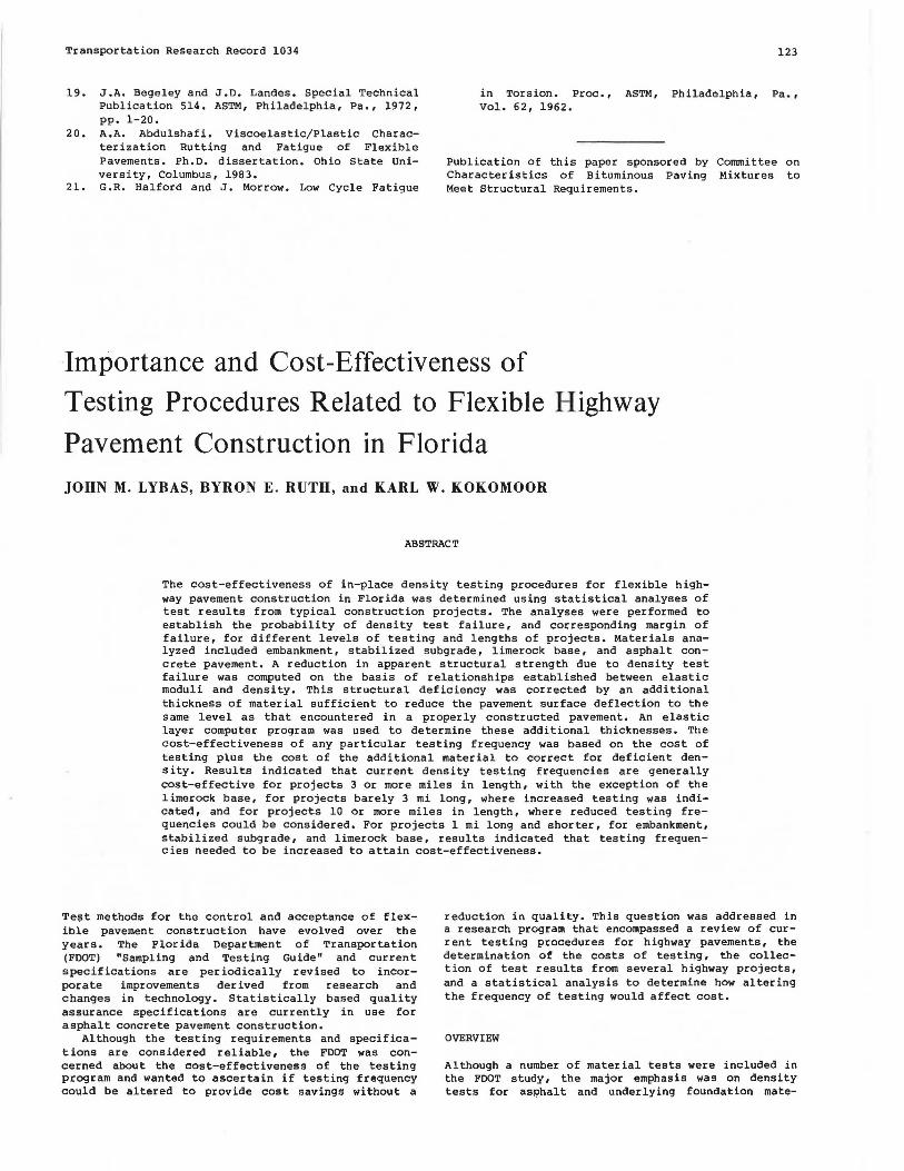
The cost-effectiveness of in-place density testing procedures for flexible high­way pavement construction in Florida was determined using statistical analyses of test results from typical construction projects. The analyses were performed to establish the probability of density test failure, and corresponding margin of failure, for different levels of testing and lengths of projects. Materials ana­lyzed included embankment, stabilized subgrade, limerock base, and asphalt con­crete pavement. A reduction in apparent structural strength due to density test failure was computed on the basis of relationships established between elastic moduli and density. This structural deficiency was corrected by an additional thickness of material sufficient to reduce the pavement surface deflection to the same level as that encountered in a properly constructed pavement. An elastic layer computer program was used to determine these additional thicknesses. The cost-effectiveness of any particular testing frequency was based on the cost of testing plus the cost of the additional material to correct for deficient den­sity. Results indicated that current density testing frequencies are generally cost-effective for projects 3 or more miles in length, with the exception of the limerock base, for projects barely 3 mi long, where increased testing was indi­cated, and for projects 10 or more miles in length, where reduced testing fre­quencies could be considered. For projects 1 mi long and shorter, for embankment, stabilized subgrade, and limerock base, results indicated that testing frequen­cies needed to be increased to attain cost-effectiveness.

Test methods for the control and acceptance of flex­ible pavement construction have evolved over the years. The Florida Department of Transportation (FDOT) "Sampling and Testing Guide" and current specifications are periodically revised to incor­porate improvements derived from research and changes in technology. Statistically based quality assurance specifications are currently in use for asphalt concrete pavement construction.

Although the testing requirements and specifica­tions are considered reliable, the FDOT was con­cerned about the cost-effectiveness of the testing program and wanted to ascertain if testing frequency could be altered to provide cost savings without a

reduction in quality. This question was addressed in a research program that encompassed a review of cur­rent testing procedures for highway pavements, the determination of the costs of testing, the collec­t ion of test results from several highway projects, and a statistical analysis to determine how altering the frequency of testing would affect cost.

OVERVIEW

Although a number of material tests were included in the FDOT study, the major emphasis was on density tests for asphalt and underlying foundation mate-