
J - Department of Statistics
153
SURVIVAL ANALYSIS FROM THE VIEWPOINT OF HAMPEL'S THEORY FOR ROBUST ESTIMATION by Steven J. Samuels '.. Department of Biostatistics University of North Carolina at Chapel Hill .4 Institute of Statistics Mimeo Series No. JUNE 1978
Transcript of J - Department of Statistics

SURVIVAL ANALYSIS FROM THE VIEWPOINTOF HAMPEL'S THEORY FOR ROBUST ESTIMATION
by
Steven J. Samuels'..
Department of BiostatisticsUniversity of North Carolina at Chapel Hill
.4
Institute of Statistics Mimeo Series No. 116~
JUNE 1978

SURVIVAL ANALYSIS FROM THE VIEWPOINTOF HAMPEL'S THEORY FOR ROBUST ESTIMATION
by
Steven J. Samuels
Department of BiostatisticsSchool of Public Health
University of North Carolina at Chapel Hill, NC 27413

TABLE OF CONTENTS
LIST OF FIGURES
LIST OF TABLES
Chapter
1. INTRODUCTION. . . . . . . . . . . . . . .
1.1 Survival Background, Parameterization ..
1.2 Description of Contents .
2. IDEAS FROM THE THEORY OF ROBUST ESTIMATION
2.1 Estimators as Functionals
Page
1
1
3
5
5
2.2 Fisher Consistency•... 7
2.3 Robustness, the Influence Curve\
The Influence Curve • . .Theoretical Considerations...Use of the I.C. with Outliers ..Assessing Robustness with the I.C.Interpretation of the I.C. in Regression.
3. EXTENSION OF HAMPEL'S FRAMEWORK TO SURVIVAL DATA •.
9
1013151516
19
3.1 Introduction.....•.. 19
3.2 The Random Censorship Model with Covariates 20
3.3 Related Work. . . . . . . . 24
3.4 Independence of Censoring and Survival •.
3.5 Limitations of Hampel's Approach ••
4. THE ONE PARAMETER EXPONENTIAL MODEL..
4.1 The Model ...
The Estimator .Functional Form .Fisher Consistency.••
4.2 The Influence Curve.
Interpretation..•.
26
28
30
30
303131
32
34

4.3 The Limiting Variance and Distribution of ~n
Page
35
4.4 Other Functions of A • 36
5. NONPARAMETRIC ESTIMATION OF AN ARBITRARY SURVIVALFUNCTION . ...•.
5.1 Note on Rank Estimators.
5.2 The Product Limit and Empirical HazardEstimators.......•.....
5.3 Functional Form: Fisher Consistency UnderRandom Censoring.
5.4 The Influence Curve ••
39
39
39
41
42
5.5 Discussion • . • • 45
5.6 The Squared I.C.
6. AN EXPONENTIAL REGRESSION MODEL
6.1 Introduction .•...
6.2 Likelihood Equations •.
6.3 The Estimator as a Von Mises Funcational,Fisher Consistency..
6.4 The Influence Curve ..
47
52
52
52
54
56
6.5
6.6
The Squared I.C. under Random Censorship.
Discussion . •
58
59
7. COX'S ESTIMATOR 62
7.1 Introduction • 62
7.2 The Proportional Hazards Model, TimeDependent Covariates.
Random Censorship.
63
64
7.3
7.4
7.5
Cox's Likelihood .•
Solvability of the Likelihood Equations ..
The Estimator as a Von Mises Functional •.
65
69
70

7.6 Fisher Consistency.
Page
73
7.7 The Influence Curve ..
7.8 The Squared I.C. under Random Censorship.
7.9 The Empirical I.C. and Numerical Studiesof Cox's Estimate •.
7.10 The Simulation Study.
7.11 Conclusions and Recommendations
8. ESTIMATION OF THE UNDERLYING DISTRIBUTION INCOX'S MODEL. . . . • .
76
84
91
105
111
113
8.1
8.2
Introduction .
Cox's Approach.
113
113
8.3 The Approaches of Kalbfleisch and Prentice
8.4 The Likelihoods of Oakes and Breslow.
8.5 Functional Form; Fisher Consistency ofBreslow's Estimator
8.6 The Influence Curve.
8.7 Estimation of G(sl~)
8.8 Conjectured Limiting Distribution forBreslow's Estimator ..•.
BIBLIOGRAPHY. .
Appendices
AI. APPENDIX TO CHAPTER FIVE••.
A2. APPENDIX TO CHAPTER SEVEN
116
119
121
123
125
127
129
133
139
A3.
A4.
APPENDIX TO CHAPTER EIGHT
COMPUTER LISTING OF SAMPLES FOR CHAPTERSEVEN PLOTS. • . • • • . . . • • • .
142
144

Figure
7.9.1.
7.9.2.
7.9.3.
7.9.4.
7.9.5.
7.9.6.
7.9.7.
7.9.8.
LIS']' OF FIGURES
Plots of the empirical influence cu~ve forCox's estimate aguinst t: n=49, a =0.36
n
Plots of the normalized differ~nce in Coxestimates against t: n=49, a =0.36.
n
Plots of the empirical influence curve for"Cox's estimate against t: n=49, 8 =1.36n
Plots of the normalized differ~nce in Coxestimates against t: n=49, 8 =1.36.
n
Plots of the empirical influence curve forCox's estimate against z: n=49, B =0.36
n
Plots of the normalized differ~nce in Coxestimates against z: n=49, S =0.36.
n
Plots of the empiri~:al influence cu~ve furCox I s estimate ag,linst z: n=49, 8 =1.36
n
Plots of the normalized difference in Coxestimates against z: n=49, B =1.36.
n
Page
97
98
99
100
101
102
103
104
LIs'r OF TABLES
Table
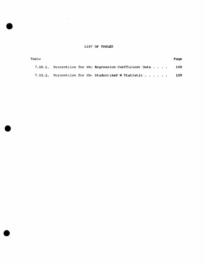
7.10.1. Percentiles for the Regression Coefficient Data .
7.10.2. Percentiles for th(' Studentized W Statistic ...
Page
108
109

ACKNOWLEDGMENTS
I am pleased to acknowledge the teaching and help of my advisor,
Professor Lloyd Fisher. The comments of Professor Norman Breslow led
to improvements in the final dr-aft, while a conversation with Ms. Anne
York was very helpful at an early stage of the work. I want to express
special appreciation to Professors o. Dale Williams and C. E. Davis,
for making possible the completion of this study. Dr. Geoff Gordon wrote
the computer programs, and Mrs. Gay Hinnant did the superb typing. To
all these I am grateful. Finally, I want to thank my parents, for their
unfailing encouragement over the years.
This work was supported, in part, by U.S.P.H.S. Grant 5-T01-GM-1269
and, in part, by u.s. National Heart, Lung, and Blood Institute Contract
NIH-NHLBI-7l-2243 from the National Institutes of Health.

1. [NTRODUCTION
Clinical trials, industrial life testing, and longitudinal studies of
human or animal populations often require the statistical analysis of cen-
sored survival data. (An elemllntary account can be found in the book by
Gross and Clark (1976). A review article with many references is Breslow
(1975). Farewell and Prentice (1977) provide advanced parametric methods.)
In this study we are concerned with the robustness of some estimators
encountered in survival analysis. In particular We extend to the censored
survival problem a formal framtlwork, due to Hampel (1968, 1974), for the
study of robustness. By robustness, we mean, loosely, insensitivity of an
estimator to deviunt data and <lepartures from assumptions. For concreteness
we will speak mostly in terms of human follow-up studies; but the results
may apply to other fields.
1.1. survival_Background, Parameterization
In survival andlysis, interest centers on time to an inevitable
response, which we term "death" or "failure." The time to failure we call
"failure time" or "survival time." (No distinction is intended.) Failure
time is modeled as d non-negat ive random variabll~ s.
Suppose we follow a sample of n persons, each with a potential failure
time S. (i=1, ... ,n). Censoring arises when S. is unobservable. This can~ ~
happen for a variety of reason:;. For example, the study may E!nd before all
n people fail; a person may drop out or move away. (A different kind of
censoring, more l.'ommon in i.ndustrial li.fe testing, is progress ive censoring.
A progressive censoring scheme is one in which the experimenter deliberately
remuves object.s from ,·.;tudy.)
2
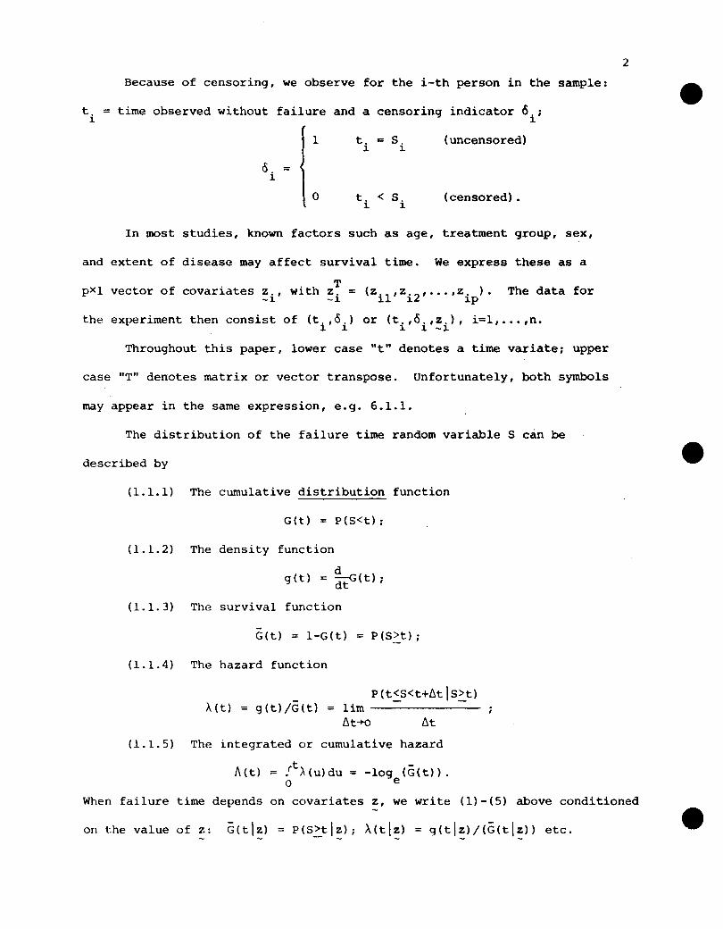
Because of censoring, we observe for the i-th person in the sample:
ti
= time observed without failure and a censoring indicator 0i;
0. =1.
1
o
t. -= S1. i
(uncensored)
(censored).
In most studies, known factors such as age, treatment group, sex,
and extent of disease may affect survival time. We express these as a
1 f · . h Tpx vector 0 covar1.ates z., W1.t z, =-1. -1.
the experiment then consist of (ti,Oi)
(Zil,zi2, •.• ,zip)' The data for
or (t"o"z.), i=l, ... ,n.1. 1.-1.
Throughout this paper, lower case "t" denotes a time variate; upper
case "T" denotes matrix or vector transpose. Unfortunately, both symbols
may appear in the same expression, e.g. 6.1.1.
The distribution of the failure time random variable S can be
described by
(1.1.1) The cumulative distribution function
G(t) = P(S<t):
(1.1.2) The density function
dget) = dtG(t) :
(1.1.3) The survival function
G(t) = I-G(t) = P(S~t);
(1.1.4) The hazard function
A(t) = g(t)/G(t) =P(t~s<t+6t IS~t)
lim--------6t-+o 6t
(1.1.5) The integrated or cumulative hazard
A(t) = ftA(u)du = -log (G(t».o e
When failure time depends on covariates z, we write (1)-(5) above conditioned
on the value of z: G(tl~)

3Inference from survival data requires the choice of models and tests
of hypotheses about parameters. These are important topics, but in this'
thesis we concentrate on estimators and their properties.
1.2. Description of Contents
Chapter 2 sketches the ~~in results from Hampel's robustness theory.
A central idea is to define est:imators based on ~l '~2' ••. '~n as functionals
of the empirical distribution function F: e =w(F). Such estimators aren n
cdlled von Miscs functionals. An estimator is Fisher consistent if
~(FO) :.:: ~, where Fa is the underlying distribution of the X's. The
influence curve (I.C.) is introduced. The I.C. is essentially a derivative
of the functional w(F) and shows the sensitivity of w(F) to local changes
in the underlying model. An empirical version of the I.C. shows how the
estimator reacts to perturbations in the data. Related theory is discussed.
"In particular, if ~e is asymptotically normal, the asymptotic variance 0 2
is often related to the I.C. by
( L 2.1)
or by a multivariatl' version ot (1.2.1) if 0 is a vector.
The general method for applying Hampel 's idl~as to censored survival
data is outlined in Chapter 3.' The idea is to write X = (t,6) or
X = (t,o,z) and define the empirical distribution function F (x) accordingly.n
We also need to model the X's dS random variables with a common underlying
distribution F(x). One such distribution is proposed, termed a random
censorship model with covariates. Limitations of Hampel's approach are
discussed, and some related work in the survival literature is reviewed.
Each of the remaining ch<1pters is devoted to a particular estimation
problem and associated estimator. Chapter 4 considers the simple

4cxponent·ial model A(t) ~ ,\ and the maximum likelihood t!l:>timator (M.L.E.) for
the model. In Chapter 5, a nonparametric eBtimator for an arbitrary survival
function G(t) is examined. Chapter 6 studies an exponential regression model
A(tl~) = exp(~T~)Ao and the corresponding M.L.E.'s.
Each of the estimators in these chapters is shown to be a von Mises
functional and, under random censorship, is proved l"isher consistent. The
influence curVe is derived, and, again under random censorship, the
relationship l.2.1 is proved.
Chapt.ers 7 and 8 are devoted to a major topic of this thesis--the
proport.ional hazards (P.H.) model of D. R. Cox (1972). In this model
>'(tlz) ~ expWTz)A (t), where A (t) is the hazard function of an arbitrary- - - 0 0
unspecified underlying distribution. Cox's estimator for 8 is examined in
detail in Chapter 7. In Chapter 8 we study an estimator (due to Breslow
1972a,b) for the underlying distribution in the P.lI. model.

2. IDEAS F'ROM THE THEORY OF ROBUST ESTIMATION
This chapter introduces those ideas from the theory of robust estima-
tion which underlie the succeeding chapters. The formal theory originated
in Hampel's doctoral dissertation (Hampel, 1968). For illuminating reviews
of robust statistics, including Hampel's theory, see Huber (1972) and
Hampel (1973,1974). There is also a brief introduction in Cox and Hinkley
(1974, Section 9.4). Hampel began by characterizing estimators as func-
tionals on the space of probability distributions.
2.1. Estimators as Functiona1s
The statistical problem is to estimate a p X1 parameter vector 8£0.
At hand are observations xl
,x2
, ••• ,xn
, possibly multivariate, with empirical
distribution function F (x).n
Definition: An estimator e for 8 is said to be a von Mises functional if-n
8 can be written as a functional of F , that is if-n n
e _. w (F ),_n n
where the functional w('), defined on the space of probability measures and
taking values in 0, does not depend on II (von Mise.s, 1947; Hampel, 1961:.l,
1974; Huber, 1972).
Exampl.es
(1) The arithmetic mean can be written
where
dF (x)n
= w (F ),n
(2.1.1) w(F) = Ix dF(x).
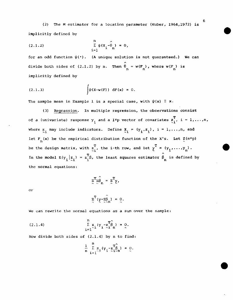
6(2) The M estimator for a location parameter (Huber, 1964,1972) is
implicitly defined by
(2.1.2)n "l: IjJ(X.-e ) = a,
i=l 1. n
for an odd function ~(.). (A unique solution is not guaranteed.) We can
divide both sides of (2.1.2) by n.
implicitly defined by
Then en
w(F ), where w(F ) isn n
(2.1. 3) f~(X-W(F» dF(x) o.
In the model E (y. Iz. )1 -1
The sample mean in Example 1 is a special case, with ~(x) = x.
(3) Regression. In multiple regression, the observations consist
of a (univariate) response y. and a lXp vector of covariates z~, i = 1, •.. ,n,1 -1
where z. may include indicators. Define X. = (y. ,z.), i ::; 1, ... ,n, and-1 -1 1 1
let Fn(X) be the empirical distribution function of the X's. Let ~(nXp)
be the design matrix, with ~~, the i-th row, and let yT = (Y1""'Yn)'
Tz.8, the least squares estimator 8 is defined by1 n
the normal equations:
or
T "Z (y-Z8 ) = a.- - --n
We can rewrite the normal equations as a sum over the sample:
(2.1.4)n T"r. z. (y.-z.a ) ::; a.
i=1-1 1 -1 n
Now divide both sides of (2.1.4) by n to find:
n "1 ~ 7,. (y.-z~8 ) = o.n i-=1"] 1 -1-n

Therefore B = w(F ), where w(F) is defined by-n n
_00
7
(2.1.5) J J ~(y_~T~(F» dF(Y,~) = o.Z _00
and Z is the domain of the z's. In this case, we can of course explicitly
solve (2.1.5) for w(F):
The reader can easily show that this gives the usual least squares solution
when F = F .n
An estimator that is not exactly a von Mises functional itself
may be nearly equal to such a functional. The sample median M , forn
example, depends for its definition on whether the sample size is even or
odd; but in large samples
(2.1.6)
The right hand side (hereafter abbreviated r.h.s.) of (2.1.6) is a von Mises
functional w(F ), defined byn
(2.1.7)
2.2. Fisher Consistency
Suppose w(F ) is a von Mises functional for estimating 8£0. Now- n
assume that the observations x1
,x2
, ... ,xn
are independent random variables,
with cornmon cumulative distribution function Fe(x).
Definition: The estimator w(F ) is Fisher consistent (F.e.) (Hampel, 1974)n
iff
~(F8) - 0, identically in 8

Remarks
1. The virtue of a Fisher consistent estimator is that it estimates the
right quantity if faced with the "true" distribution.
2. The definition given abovt' is the one used by Hampel (1968,1974) and
others. Rao (1965, Sc.l) requires in addition that w(-) be a weakly
continuous functional over the space of probability distributions.
3. Fisher consistency does not refer to a limiting operation. Fisher
consistency and ordinary weak consistency (convergence in probability)
cannot be related without regularity conditions on w(-) and the space
of probability distributions.
4. The parameter 8 need not completely identify the distribution FO.
Examples
8
1. Consider the family of distributions F with finite first moment ll.II
Then the functional (2.1.1) evaluated at F givesII
w(F ) = Ix dF (x) == ll.P II
Therefore the arithmetic mean is F.C.
2. In the regression sptup of Example 3 in Section 2.1, let the
covariates z be drawn from a probability space Z with distribution function
K(z). Conditional on z, draw the response y from a distribution GS(yl~)
such that
E I (y\z) -= Jy dGo(y\z)y z - p-
'l'hpn the joint dist.ribution of (y,z) is
Tz (~.
If this distribution is substituted in the normal equations, (2.1.5), one can
easily show that w(F) S is a solution. (Details are left to the reader).

9Therefore, the least squares estimator w(F) defined by (2.1.5) is, under
this model, Fisher consistent.
2.3. Robustness
Hampel chose to study an estimator w(F) in terms of its functional
properties. For example, the natural requirement that w(F) estimate the
"right thing" is translated, in functional terms, into Fisher consistency.
"Robustness" is identified, in part, with stability of w(F) to changes in F.
As outlined by Huber (1972) and Hampel (1974), there are three aspects to
this stability: continuity of the estimator, its "breakdown point," and
sensitivity to infinitesimal changes in F.
Continuity is the requirement that small changes in F (errors, con-
tamination, distortion) lead to only small changes in the estimator w(F) .
Formally, a metric is introduced onto the space of probability distributions,
and continuity of w(F) in this metric is required. The Prokhorov metric
is often convenient for studying robustness, though other metri.C's can be
used (Prokhorov, 1956; Hampel, 1968,1974; Martin, 1974). Among familiar
estimators, the sample mean defined by (2.1.1) is nowhere continuous in the
space of distributions.
The breakdown point is, roughly, the smallest percentage of observa-
tions that can be grossly in error (at ~ 00, say) before the estimator
itself becomes unbounded. For example, the breakdown point of the mean is
zero; that of the median is 50 percent. Again, there is a formal definition
in terms of the Prokhorov metric.
The Prokhorov metric proves difficult to work with in the survival
setup of the next chapter. Therefore, we will not formally study con-
tinuity and the breakdown point in this thesis. Instead we concentrate
on the third aspect of robustness--stability of w(F) in the face of local

or infinitesimal changes in F. This leads naturally to consideration of 10
a "derivative" of w(F) at F and consequently to the influence curve.
The Influence Curve
The influence curve (I.C.) was introduced by Hampel (1968). Among
published discussions are an expository article by Hampel (1974) and
sections of Huber (1972) and of Cox and Hinkley (1974, Sec. 9.4).
Most applications of the I.C. have been to estimation of univariate
location and scale (Andrews, ~! al., 1972). For mUltivariate applications
see Mallows (1974) (regression and correlation) and Devlin, Gnanadesikan,
and Kettenrinq (1975) (correlation).
We first. define a general first order von Mises derivative. Let F(x)
and K(x) be probability measures on a complete, separable metric space.
Suppose w(0) is a vector valu('d von Mises Functional (estimator). Form
the (-mixture distribution F£ (l-C)F + £K. For sufficiently nice F, the
estimator w(o) has a von Mises derivative at F:
£(2.3.1) U~ w(F)J =
d - ££ £:;0
w(F ) - w(F)1 , - £1m _
£-..0
for some function IC(x;w,F) (von Mises, 1947; Filippova, 1962, Hampel,
1968) .
In particular, we can find I_C(XiW,F) by letting K(x) =
distribution function which puts mass one at x.
I , thex
(poi.ntwj~;e) <it 1S i~; given by:

11
(2.3.2)
£
where F £ = (1-£) F + £ Ix'
Example 2.3.1 (means)
Let
~[(l-£)F + £ I 1lim x
£~
w(F) = EF(~(x»
J~(U) dF(u),
- 't(F)
*for some function b(x). Then, contaminating F with the point x , we have
w(F ) = J~ (u) d[(1-£) F + £ I * ] (u)c x
J~(U)dF (u) *= (1-£) + £b(x )
*= w (F) + £[b(x ) -w(F»).
And
Therefore
w(F ) - w(F)~ £
£w(F) - b(x) (ve:>O) •
(2.3.3) * *Ie (x ; w , F):: b ( x ) - EF
(b ( x) ) •
When F = F , the empirical I.C. of the sample mean (b(x) = x) isn
(2.3.4)
Remarks
IC(XiW,F )n
x - Xn
1. If w(F) is a pXl vector valued estimator, ~(F)T '" (W1
(F),W2
(F), ... ,Wp
(F»,
the IC(x,w,l") is also a pXI vpctor. The k-th coordi.nate of the IC is

(2.3.5) Ie (XiW,F) '" IC(xiwk,F).k-
] 2
That is, ICk
is just the I.C. of wk'
2. Let us note for future use that L=O corresponds to the "central case":
3. How does the I.C. express Lhe "influence" of un observation on an
estimator? For one answer, we consider the empirical I.C. for a sample
with d.f. F. Let w(F ) bt~ the estimator based on F and x a possiblen n n
observation (not necessarily in the sample). Form F = (l-£)F + £ In,E n x
A first order Tay1or.'s series expansion about w(F ) using (2.3.2) givesn
(2.306) w(F ) - w(F ) == L IC(XiW,F ) .. 0([").n,L n II
l/n+1. Tht'n each of the observ,ltion~; x. (i=1, ... ,n),1
which in Fn hud mass J/n, hilS in Fn ,J/(u+1) mdSS
(1-£) /n 1/ (n+1) .
The "new" observation x ha~; mass
f = 1/(n+1).
Therefore, the mixture dis1.ribution F is the distribution ofn,l/(n+1)
+xthe samplt~ of: size !~+l., F
n+
J, say, consisti.ng of x1, ... ,x
nand x.
( +x ) .. hThp esti.mclt.or w(F / » == w FIlS the (~st1.mat.or based on t. en,l (n+l n+
dugmpntt'd sampll', dnd the t'xpansion (2.3.5) becomps
(2.3.7) W(f'+x\) - w(F )n+ n
IC(XiW,F )n
n+J+ O(l/(n+1) 2).
Approximately
(2.3.8)+x
(n+l) Iw(F l)n+.
w(F ) 1n
IC(xiw,F ).n
In other words, the empirical I.C. measures the normalized change in
the estimator caused by tht· addit. ion of a point x to the sample.

13
For the case of the sample mean w(F ) = x , one can easily shown n
x-xn
n+1
That~ is, the rcl.ationship (2.3.H) is exact. In other cases, where w(F)
is not linear in 1", (2.3.8) may provide only d qualitative approximation.
(The approximation will be examined in Chapter 7 for the case of Cox's
estimator.)
4. If (2.3.]) holds, then
(2.3.9) o.
In particular, when F = Fn
(2.3.10)II
r. IC(x. ;w,F ) = o.i=l 1 - n
For the estimators examined in this study, we will not prove the
existence of tlw general von Mises derivdtive sat i sfying 2.3.1. But
equations (2.3.') and 2.3.]0) will be checked for the I.C.'s d(~rived
in the chapters to come.
Theoretical Considerations
When the general von MiSt'S derivative (2.3.1) exists, another Taylor
series expansion may hold.
(2.3.11) w«l-c)F +£K) - w(F)
This leads to d proof of the a~;ymptotiG normality of 0 = w(F) (Cox and-n n
Binkley, \974).
1/11 and let K(x) = ni" (x) - (n-1) F(x).n
Then
P (l-L) P +l. K ~ F and( II
Jrc(X;~,F) dK(x)
w; i Ill) (2. 3.9) .

14
The n by ( 2 • 3. Ll)
(2.3.12) w(F ) - w(F)n
n
= (l/n) .}: I_~(xi;~'I") + O«]/n)2).1-"]
Note that the 1. C. with respect. to F, not F , appears on the r. h. s. ofn
(2.3.12) Here IC(X.iW,F) expn'sses the "influence" of x. on w(F) in1 - 1
a way d liferent from (2.3.7). The summands IC(X.iW,F) are i.i.d. random- 1-
v<..lriables with mean zero (by (:>..3.9) and variance-covariance matrix
TE (JC(x,;w,F) IC(X.iW,F) )
F - J -. - 1-
(2.3.13)
Appeal to the central l.imit th.'on!m leads to the conclusion that
U.3.L4) ;;-; (w (F ) - w ( F» ~ N ( 0 , A (w , 1") ) •- n·· ~ • -
'rill' l·oll<.lilion~; under whie'll (2 ..LI4) ho.Ldu h,)v.' bel'lI dlBcusBod by
VOII MiHt'H (llJ47), !"iliI'Povu (illbl), und MUII'r and Sun (llJ7:l). Ttll! ('on-
ditions are so IlC,.1Vy t.hat in pJ'CJ(;ticp, asymplot.ic l1ormalit.y if::; usually
proved by other means.
When asymptotic normality has been proved by other theory for estimates
ill succCl~ding dl<..lpt.l'rS, we will check that l\(w,F) agret's with the limiting
covarianc0 mat.rix.
A sample approximation to l\(w,1") is (for p=l)
(2.:L 15)n
l\(w,F ) =- 1/11 ): TC~ (x. ;w,F ).fI i=1 1 n
'l'hj~. cstimatL' of l\(w,l<') is dis('u5~H.'d by Cox ,wd Hinkley (1975) and by
Mal lows (1974).
For one I!St. imdtor st uelled in thiH thes is, till' Breslow Cot imate of the
underlying dj!;tribution in Uw Cox modol, Chapter II, no limi.ting result.s are
known. In th is case we wiJ 1 ~~l!~~-,.::t~~ that asymptotic norma.1 i ty holds,
15
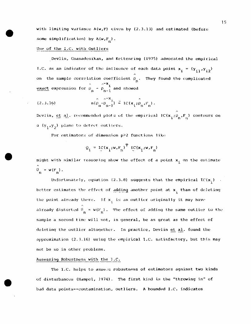
with limiting variance A(w,F) qivl'n by (2.3.13) and estimated (before
some simplification) by A(w,F ).n
Use of the I.C. with Outliers
Devlin, Gnanadesikan, and KeLtcnring (1975) advocated the empirical
I.C. as an indicator of the influence of each data point Xi = (YiI'Yi2)
on the sample correlation coefficient p. They found the complicatedn
.,,-x.. 1.
exact expressIon for p - P 1 and showedn n-
A-X ..1 ~
n (p -p ] ) IC (x. i P , F ).n n- 1 n n
Dev 1 in, et al. ['(-commended plot S 0 f t.he f~mp i r i<,:a} JC(x.;P ,I" ) contours on1 n n
For estimators of dimension p>2 functions like
TQ. = lC(X.iW,F) IC(Xiiw,F)1- 1 n - n
might with similar reasoning sllow t.he effect of a point x. on the estimate1.
o w(F) .n n
Unfortunatl:'ly, equation (2.3.8) suggests that the empirical IC(x.)1.
better estimi.lt.es the <,ffpet of ~~~i.-n~ another point at x. than of dl>] et.inq1.
t.he point already there. I f' x. is an out.] ier originally it may haw'1
already distorted II = w(F ). 'I'hc effcct of adding the same outlier to t.hL'n n
si.unple a second t im(; wi 11 not, :i n general, be as great as the effect of
deleting the outlier altoqethel. In practice, Devlin et al. found the
approximat ion (2. J .16) usi ng the l~mpirical 1. C. satisfactory, but thi s may
not. be so in other problems.
Assessing Robustness with the l.C.
The I.C. helps to asse.;s robustness of estimators against two kinds
of disturbances (Hampel, J974). The first kind is the "throwing in" of
bad data points--contamination, outliers. A bounded I.C. indicates
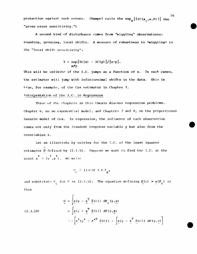
protection against such errors.
"gross error sensitivity.")
16(Hampel calls the sUPxIIIC(xi;w,Fl II the
A second kind of disturbance comes from "wiggling" observations:
rounding, grouping, local shifts. A measure of robustness to "wiggling" is
the "local shift sensitivity":
A = supIIC(x) - IC(y) I/Ix-yl.x,/y
This will be infinite if the I.C. jumps as a function of x. In such cases,
the estimator will jump with infinitesimal shifts in the data. This is
true, for examplp, of the Cox pstimator in Chapter 7.
'I'hn.'(.' of the chapters in this thesis discuss n~grE'ssion problems.
Chapter 6, on an exponential model, and Chapters 7 and 8, on the proportional
hazards model of Cox. In regression, the influence of each observation
comes not only from the (random) response variable y but also from the
covariables z.
Let us illustrate by solving for the I.C. of the least squares
estimator Bdefined by (2.1.5). Suppose wp want to find the I.C. at the
* * *point x = (y ,z). W<' writ.!'
F ( I -I") F + F r *I X
and substitute Fl
then
[or F in <2.1.5): The equation defining f3(E;) = w(F ) is£
J:(y TB(f.) ) dF£(y,~)0 - z
(2.3.18) I: ()' T B(E) ) dF(y,z)- z
r * *.T B(n) hey T B(,') ) dF (y , ~)1I Z Iy - z - z

Now differentiate (2.3.18) w.r.t. (: and evaluate at £=0. This gives,
(using 2.3.9),
17
(2.3.19)
Or
* * *T+ z Iy - z S(O»).
* *IC(y ,z ;l3,F)
( 2. 3.20)
when F = F , 8(0)n
is therefore
IfT -j-l * * _z *T Q «» 1
:: dF(y,:) ~ (y ....
B(F ), the loS. estimate based on F. The empirical I.C.n n
(2.3.21) * *IC(y ,z d3,F )- - n
T -1 * * *T A
n (Z Z) z (y - z S) •-on
This implies, that
(2 ..3.22)
(2.:L 23)
A * *It(y ,l, )"n-tl
- n T -1 * *(--) (Z Z) z (yn+ 1 ",."
T -1 ." *(Z Z) z r
*where r y * *'1'- z l3
-n* *We see that the point (y ,z ) influences the estimate B in two ways.
*One, as expected, is by means of the discrepancy between y and its
*Tpredicted value z S; this discrepancy is measured by the residual
-n
*r y * *T A
z l3-n
The second way is by means of the magnitude of the
*independent variables z. EVlm if the residual is slight, extreme values
*of z may strongly affect the estimate. Hampel (1973) calls this effect
*of z th(~ "infllll'nCe of pl)~1ition in factor space."

Errors in the data may give rise to large residuals, but a
*(relatively) large z may not be an error at all. We may nonetheless
18
want to make an estimator robust against the influence of z's far from the
data (Hampel, 1973; Huber, 1973). This influence can stand out strongly
in estimators that are otherwise robust (e.g. the Cox estimator, based
on ranks, in Chapter 7).

3. EXTENSION OF HAMPEL'S FRAMEWORK TO SURVIVAL DATA
3.1. Introduction
In this chapter we 5how how Hampel's ideas can be applied to censored
survival data with covariates. In the last part of the chapter, some other
work on the robustness of survival estimators is reviewed.
Application of Hampel's ideas first requires definition of an
empirical distribution function F. Recall from Chapter 1 that in an
for each patient: t. is the observed time on study, 6. is a censoring1 1
indicator (0 = censored, 1 = uncensored), and ~i is a vector of covariates.
We therefore find it natural to make the following definitions:
Definition 3.1.1. The observations in the survival problem consist of
vectors x. ,x2
, ••• ,x , where1 n
x. (t"6,,z.)J 1 1-1
if covariates are present; and
if covariates are not present. To simplify notation the wavy underscore is
omitted from the x's, though Hot from other vectors, throughout this
dissertation.
Definition 3.1.2. The empirical distribution function F (x) based on the-'-..----- ------- ----- -n--
sample xl
,x2 " .. ,xn is that distribution function which puts mass lin at
each observed x. (i = 1, ••• ,n).1
With F defined, we can study survival estimators as von Misesn
functionals w(F ).n

3.2. The Random Cens_orship Model with Covariates
Application of Hampel's theory also requires that the observations
xl
,x2
, ... ,xn
be modeled as Li.d. random variablf~s with distributi.on
20
function Fe. (Here e is the parameter to be estimated.) This allows
consideration of Fisher consistency and properties of the influence
curve with regard to an underlying distribution.
This requirement poses a problem: In survival analysis, the only
distribution specified is Ge(s I~) (or Ge(s), a special case), the dis
tribution of the failure time random variable S: the only ~Emeter..:?_ of
-interest are p~rameters of GO' The observations x ~ (t,O,z) depend, how-
ever, not only on GO but on the occurrence of censoring and on the
covariates z. The mechanisms generating the censoring and the covariate
are arbitrary nuisance mechanisms, which may not be random at all. The
data can therefore arise in many ways.
To apply Hampel's ideas, we define a distribution F(x) in which the
censoring and covariates are random but otherwise unspecified. This dis-
tribution is an extension of t.he model of random censorship (Gilbert, 1962:
Breslow, 1970: Breslow and Crowley, 1974; Crowley, 1973). We may t:herefore
call this new model the !andom. .ce~sorship !!:.odel ~ith covariates (and where
Definition 3.2.1. 1\n observat.ion x. "" (t. ,l). ,z.) from the random ('ensor-1 1. 1 -1.
~,hip model is lIt'nerated in th" following steps:
1. The z. are a random sample from il distribution with d.L K(~)~l.-
on domain Z. We may assume that the distribution has a density
k(z)dz = dK(z) (defined suitably when z contains both continuous
and discrete elements).
2. Obtain the failure t lme S. from G(slz.) with density g(s\z.) ,Where1 ~l. ".1
z. was generated as in (1).~l

213. Independent of step (2) pick the censoring time C
ifrom a distri-
bution H(c lz.)-1.
with H(c\Z.) =-1
= p{c<clz.},-1
1 - H(clz.).-1
with density dH(clz.) = h(clz.), and-1 -1
Again z. is from step (1). In-1
other words, Ci
is, conditional on ~i' independent of Si·
4. Form t. = mineS. ,C.) and o.111 1
tor of the event A).
5. Then x. = (t.,O. ,z.) and the resulting distribution function is1 1 1-1
F (x) •
If there are no covariate~~, the process consists of picking Si and Ci
independently from G(s) and H(c) respectively, and of forming (ti,Oi) as
in steps (4) and (5).
We can calculate expressions for the joint distrihution f(t,o,z) as
follows. For the moment, let upper case "T" denote the random variable,
while lower case "t" denotes a particular value.
P(T<t,O=ll:) = P(S<t,s<cl~)
t
= J H(yl~)g(yl~)dY.o
The conditional density is found by differentiating the last
expression with respect to t:
We will denote this f(t,ll~)
(3.2.1) f(t,O=ll~) = H(tl~)g(tl~).
dF(t,ll~)
dt
Then
f(t,l,z) ~ f(t,ll~) k(~)

Similarly, 22
()F(t,O,z)where, again f(t,O,z) '''' --J:-~-- is "hort for f(t,o==O,z).
utaz
The total density, with respect to the product of Lebesque and
counting measure, is
(3.2.3)
(3.2.4)
f(t,o,z) [H(t!:)g(tl:)]O [G(tl:)h(tl:)2l-0k(:)
I 0- I 1-0 I 0- I 1-0[get ~) G(t:) ] [h(t :) H(t:) lk(:).
In estimation problems, the parameters of interest are parameters
of G and g. The factorization of f(t,o,z) is noted only implicitly and
only the first term
(3.2.5) I 0- I 1-0get :) G(t :)
appears in the likelihood.
The symbols F ilnd f will designate marginal, conditional, and uncon-
ditional distributions of (t,O,z). Thus we write
f (t, 1)(3.2.6) ~F~~,_u.. == J f(t,l,~)dK(:),Z
for the marginal density of observed failure times. We will always assume
enough regularity so that integcations in t,z, or in C,S, and z can he
performed in any order.
Derivations, when there are no covariates, are easily made.
Remarks
1. This random censorship modet with covariates WetS inspired by E'nrlier
work of Breslow (1970). Brt~slow studied a generalization of the Kruskal-
Wallis test for comparing survival distributions of K populations. The
long run proportion of obsecvations from the j-th population was
K
A. ( E A,==1); and a different censoring distribution was allowed forJ j==l )
each population.
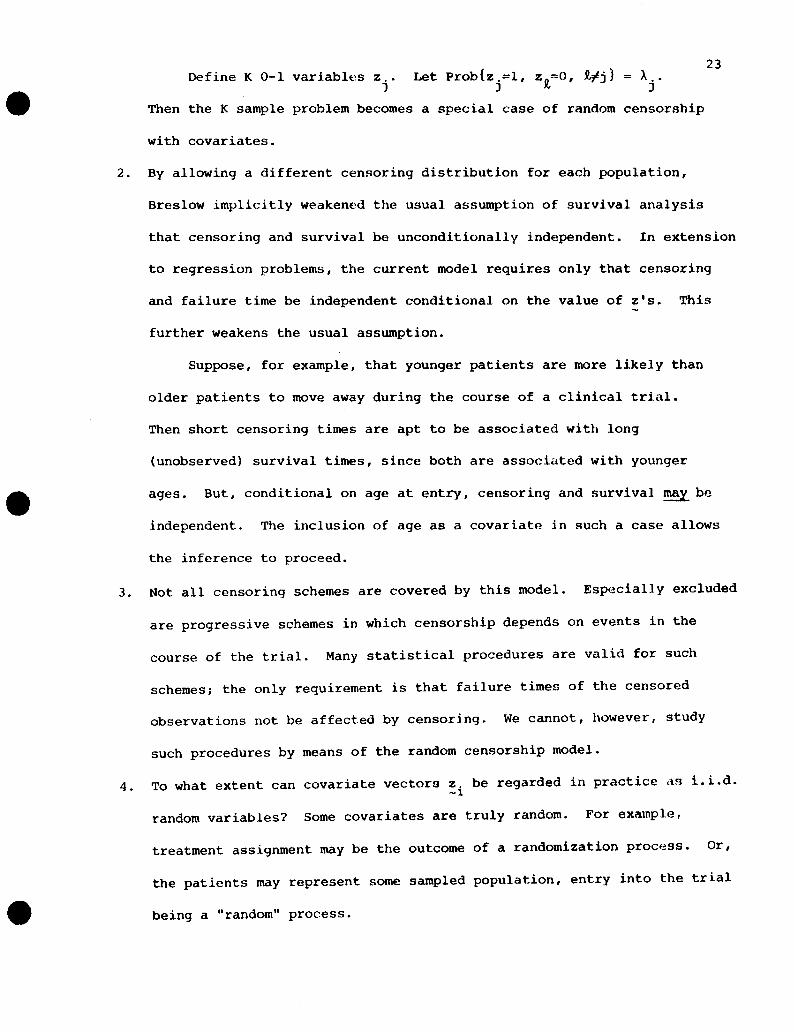
Define K 0-1 variables Zj' Let prob{Zj=l, Zl~O, ~j} = Aj
.
Then the K sample problem becomes a special case of random censorship
with covariates.
23
2. By allowing a different censoring distribution for each population,
Breslow implicitly weakened the usual assumption of survival analysis
that censoring and survival be unconditionally independent. In extension
to regression problems, the current model requires only that censoring
and failure time be independent conditional on the value of ZI S • This
further weakens the usual assumption.
Suppose, for example, that younger patients are more likely than
older patients to move away during the course of a clinical trial.
Then short censoring times are apt to be associated with long
(unobserved) survival times, since both are associated with younger
ages. But, conditional on age at entry, censoring and !'iurvival may be
independent. The inclusion of age as a covariate in such a case allows
the inference to proceed.
3. Not all censoring schemes are covered by this model. ESp(~cially excluded
are progressive schemes in which censorship depends on events in the
course of the trial. Many statistical procedures are valid for such
schemes; the only requirement is that failure times of the censored
observations not be affected by censoring. We cannot, however, study
4.
such procedures by means of the random censorship model.
To what extent can covariate vectors ~i be regarded in practice
random variables? Some covariates are truly random. For example,
1. Ld.
treatment assignment may be the outcome of a randomization process. Or,
the patients may represent some sampled population, entry into the trial
being a "random" process.

24At the other extreme <lrE' covariates which are fixed. The need for an
intercept in a regression mod(~l, for· example, may require a covariate
z .. - 1. We may think of this covariate value as being sampled with1)
probab il ity one.
Between the t'xtremes of truly random and truly fixed covariates are
others, in which t.he sampled distribution may be hard to describe at
best: patient assignment schemes, "balancing" of patients within
treatments, biased or arbitrary recruitment and selection. In such
cases (which are cormnon), we would only conjecture that the covariates
behave like random varidbles wit.h some regularity conditions.
5. In Cox' oS (lC)72) regn'ssion model, the covariate values may change with
time. Such covariates may also be considered in a random censorship
model. 1\ di scussion is <]('fer-red unt i 1 Chapter Seven, where the study
of Cox's model takes placf'.
3.3. Related Work
In this section, some rplated work on robm;tness in the survival
literature is outlined. 'l'hesp references do not constitute a complete
survey; they are intended only to alert the readf'Y to other approaches.
Fisher and Kandrek (197'la) studied the extent to which choic{' of
incorr('C't model ;lffccted illfer('lIl'(' in f;lIrviv,ll "IIdlysi!C;. They studied four
exponent ial regre~;~;ion models. with Ute distribut i 011 dcpelldinq on one
covariate z:
1. A1 (z)
2. \.~ (z)
3. A (z)J
4. A4
(Z)
1/(0 + l~ z), Felq.1 and Zelf'1l (l<.)()5).o 1
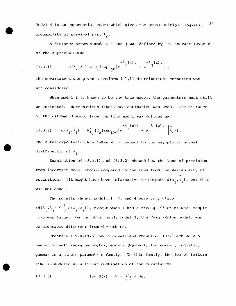
Model 4 is an exponential mo<1('1 which qivp~; the usual multip.le logistic
probability of survival past to'
'".L.:J
A distilnce bf'twf'en models i dnd j W3!'; dl'firll'd by !h(· ,lv('cdqe (over z)
of the supremum norm:
(J.3.l) d(A"A.).1 1
-'\,(z)t
E (su1> II' 17. t>O
-A.(Z)t
.1 I).- e
The covariate z was given a uniform (-1,1] distribution; censoring was
not considered.
When model i is known to be tlw true model, the parameters must sti 11
be estimated. Here maximum likelihood c!;t.imation was used. The distance
of the cstimatf'd model from tll(~ tru£' model was ciefint~d its:
(3.3.2) dO,.,A.).1 1
-A.(Z)t~ I 11':\ (E (~;up >0 ('(\ . z t
1
-A.(Z)t I"-e 1 1\).
'I'hl' outer expecLltioll wa~; Llkt'n with respect to the asymptotic normill
distribution of A..1
Examination of (3 ..1.1) ilnd (3.3.2) showed how the loss of precision
from incorrect model choice compared to the loss from the variability of
estimation. (It might have b('en informativp to compute d(A .. ~,.), but this) 1
Waf) not done.)
Th(' re~;1I1 t~; sh()w,-~d mode l~; I, J, and 4 wen' vpry c I OS('
I ~
(el(A.,A,) <_. tI(A.,A.)), "xc!'},t wh(~n z h(ld d stconq t'ffl.'ct or wht'l\ sample1 1 .3 1 1
:;i7.e was LHqP. On the other h.Jnd, model 2, thp i"f·iql--·7,(']en model, was
considerably di ff('rent from tile uthccs.
Prentice (1974,1975) and Fan'well ann Prentice (ll)'17) embedd('d i1
number of well known parametric models (Weibull, log normal, logistic,
gamma) in a !;inqle parametric family. In this family, the log of failure
time is modeled as <1 line,lr combination of the covdriates:
(1.3.3) log S (z) a TZ('1 + p + Ow.

Here a is a scale parameter and w is an error random variable.26
According to
the generality required, w follows eithpr the distribution of the log of a
ganuna R. V. (one parameter) or the log of an F' random variable (two
parameters). Censoring is taken into account; likelihood methods provide
tests and estimates. Prentice and Farewell show that inference about B
may be more robust to spurious response times, if the model (3.3.3) is
fitted.
Independence of Censoring and Sur_vival
Most procedures in survival analysis depend upon some kind of
assumption of the independence of censoring and survival. (In the random
censorship model, we require independence conditional on z.) The assumption
enables one to factor likelihoods, so that estimation of the survival
-function G can proceed.
In many applications, the assumption of independence is suspect.
Patients who drop out of clinical trials may De more sickly than those
who stay in, or they may be hE·althier. For example, patients who drop out
because of drug side effects may be constitutionally different from those
who do not suffer such side effects. Or, patients who are healthier may be
better able to move away from the city in which a study is located.
What are the consequencE's for survival analysis? This question has
been studied by several authors. Peterson (1975) and Tsiatis (1975) in a
competing risks set-up proved the following: that any underlying distribu-
tion F(t,O) (or F(t,O,z» of the observed data may arise from an infinite
number of survival distributions G, if dependent censoring is possible.
Therefore G is not identifiilble.
-Peterson studied nonparametric estimation of G via the Kaplan-Mei.er
estimate (described in Chapter Four). He obtained sharp upper and lower

27bounds for the estimate. The lower bound is equivalent to designating all
censored observations as failures immediately after censoring. The upper
bound is found by treating all censored observations as if they never fail.
For some data sets (in which there is little censoring) the bounds can be
narrow; with heavy censoring they can be wide.
Fisher and Kanarek (l974b) also studied the problem of estimating a
-single survival function G, when censoring and failure time are dependent.
TIley presented a model with two kinds of censoring. The first kind was
"administrative" censoring caused by end of study; such censoring should
be independent of survival. The second censoring was loss to follow-up
due to dropping out. In the model, such loss to follow-up affected failure
time through a non-estimable scaling parameter, 0 ~ a ~ 00. Large values
of a (>1) corresponded to poor survival, following censoring; small values
«1) corresponded to better survival. The extremes of a=O and a::ro
corresponded to Peterson's upper and lower bounds, respectively, while
a=l was equivdlent to independence. By varying a and finding the M.L.
estimate of G for each value, an investigator could asspss the rob\l~tness
of his estimates to the indep{.·ndence assumpt ion.
Fisher and Kanarek also discussed ways of using auxiliary information
to test the assumption of indE'pendence. Suppose that at time t., N. peopleJ J
are being followed and K. of these are lost to follow-up (in some smallJ
interval following t.). If the assumption of independence holds, any setJ
of K. people of the N. at risk might, with equal probability, have beenJ J
lost. If the assumption is not true the covariate values for the K.J
who were lost should be somewhat separated from those who were not lost.
These facts are exploited to give tests of the independence assumption.
The appllcabi lity uf thl'5e results in regression problems is not
cloar. Certainly one can apply til£' trick of failing censored ubservdtions

28at the time of censoring or of letting them live forever. This should be
easy to do and to program on a computer. Perhaps an analogue of Fisher
and Kanarek's (l974b) a-technique can be extended to the regression problem;
this might provide a more realistic assessment than the extreme bounds
(corresponding to a=o and a=oo).
3.5. Limitations of Hampel's Approach
First consider the estimation problem when there are no covariates.
We would like to study the continuity of O=w(F) with respect to changes in
G, the survival function. We are restricted to studying continuity with
respect to changes in F, the argument of the functional w. Results quoted
in the last section show that the same F may correspond to many different
survival distributions G, if censoring and survival are not independent.
This nonidentifiability property makes a general study of continuity
extremely difficult. ~I
One approach is the following: Assume that rdndom censorship holds
(thus ensuring independence of failure and censoring times). In addition,
assume that the censoring distribution H(c) is fixed. The resultinq
distribution F of x=(t,6) should be a 1-1 functional of G: F=q(G), say.
The estimator is then also a functional of G, defined by neG) = w(q(G).
The formal study of the functional n=wOq can then proceed; we shall not,
however, do so.
With covariates, the situation is more complicated. We cannot define
the estimator as a functional O=fj(G), because there is no single underlying
G. Instead there is a different distribution G(·I~) for each value of the
covariables z. In regressiun problems, therefore, the functional approach
if> restricteJ to st.uJy of U""w(F).

29The restriction of Hampel's ideas to estimation is another limitation.
Some extensions to test statistics are possible, but we will not pursue the
subject in this study.
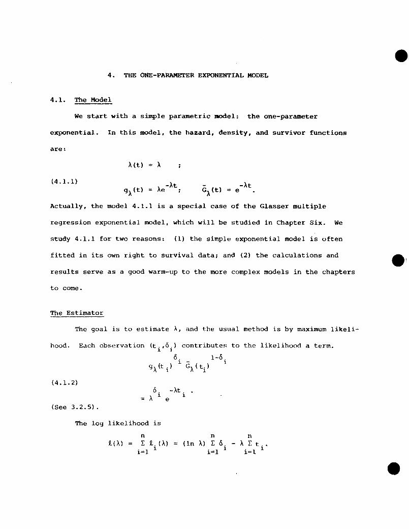
4. THE ONE-PARAMETER EXPONENTIAL MODEL
4. 1. The Model
We start with a simple parametric model: the one-parameter
exponential. In this model, the hazard, density, and survivor functions
are:
A(t) :: A
(4.1.1) -Ate
Actually, the model 4.1.1 is a special case of the Glasser multiple
regression exponential model, which will be studied in Chapter Six. We
study 4.1.1 for two reasons: (1) the simple exponential model is often
fitted in its own right to survival data; and (2) the calculations and
results serve as a good warm-up to the more complex models in the chapters
to come.
The Estimator
The goal is to estimate A, and the usual method is by maximum likeli-
hood. Each observation (t. ,6.) contributes to the likelihood a term.1. ]
6. 1-6.1. - 1
gA(ti
) G).(ti
) .
(4.1.2)6. -At. •
:: ). 1. e 1.
(See 3.2.5).
The log likelihood is
nt(A):: E t. (A) ::
i=l 1.
n n(In A) E 6. - A E t ..
i=l 1. i=l 1.

.H
The estimatiny equation :is therefore
nd
n n(4.1.3) ): V. (A)
dAY.Pd = )~ o. - E t. = 0,
i=ll.
i=l l. i=lJ.
AO.
where Vi (A) = Al. - ti
is the efficient score for a single observation.
Equation 4.1.3 is solved by
An
n nLO./Lt ..
i=l l. i=l l.
>. is the ratio of the observed number of failures to the total exposuren
(4.1.4)
time in the sample.
Functional Form
Let 1" be the s.:lmplp dist ribution fWlCtion of (t,l). A can bl~n
written
A1 1
= (-r.0 . ) / (-}: t . )n n 1. n l.
(4.1.5)
= Io dFn(O)/[t dFn(t),
= l\(F ) /B (1" ), say,n n
wlwre A(F) EF' «(.\) , B(F) = EF
(1) • Therefore A = w(F ) , withn n
(4.1.6) w (l~) A(1")/B(f') •
!::_lsher Consislcn<..:y
Let Hk) bp an urbitrary distribution of cem;oring time. With the
model 4.1.1 for failure timp.s, a random censorship model (without covariates)
is easily defined, uS in Section 3.2. Let F>.(t,O) be the resulting distribu
tion of the data. Fisher consistency will hold, if

32
We show this by evaluating A(FA
) and B(FA), which are the expectations
(over 1'\) of 0 and t, respt!ct.ively:
A(FA) = EF
(0) = p{s<c}A
(4.1.8)00
= J H(t)gA(t)dt
o
00
J- -AtA H(t)e dt.
o
(4.1.9)
00
B(FA) = EFA
(t) = f (I-FA(t)dt). (Rao, 1965, 2b2.1)
o
I-FA(L) p{S>t} p{c>tl, by independence,
(4. L 10) = G,\ (t) 11 (t)
-Ate H (t) •
Therefore,
(4.1.11>
and
4.2. The Influence Curve
00
J-At-
e H(t)dt,
o
Suppose we cont,iminute d distrihution F' with a point x ~ (t,6). We
Writl' the contdmillcited di::;ldbution as Fc = (l-c)F' +f:I1x1
' where Ilxl is
the c.d.f. which puts mass 1 at x.
The estimator of the exponential hazard based on F is:(:
(4.2.1) w ( F ) = A ( F ) /8 ( F ),£ £ I::
or, to simplify notation:
(4.2.2) w(c)

BIOMATH£MATlCS TRAtNING PROGRAM
The influence curve is given by:33
(4.2.3) IC(x;w,F) = :i w(C) Ic~o =B(O)A' (0) - A(O)B' (0)- B 2 (0)
where 1'.'(0) :::: ?d 1\«(:)1 0 etc. and 1\(0) :::: An'). 'fhe derivatives A'(O)C L=
and B'(O) are easy to evaluate from (2.3.3), since A(F) and B(F) are
means:
A' (0) = <5 - A(F)
(4.2.4)
B'(O) = t - B(F).
Simplifying (4.2.3), we find
1('( (t,cS) ;w,F)
(4.2.5)
= 6 - [( A (F) /B (F) 1t:_Bn')
<5 - w(F)t------_.B (F)
The ~mpirica1 I.C. is found by substituting Pn
for P in (4.2.5):
(4.2 •. 6) IC( (t,o) ;w,F )(I
o - A tn
B<J.T =n
6 - A tn
tn
Check on Computatio~
By (2.3.9), an I.C. should satisfy EF(IC(x;w,F» = O. We can easily
show this for the I.C. (4.2.5). By definition, we have for any F,
Ep
(0) = A ( F), EF
( t ) "" B ( F) • By ( 4 • 2 • 5)
E (I C ( (t ,0) ; w , f') = E {.o - (A (F) /8 (P) ) t.}F F B(P)
(4.2.7)
:::: (A(Fr - A(F'»/B(F) = O.
The argument ctbove holds for 1"= 1.0' so thatn'n~ IC(x.;w,F ) = 0,
i=l 1 n
which is (2.3.10).
o

34
Interpretation
The influencE;' curve~ for the estimated hazard rate are fairly easy
to interpret. We go into some detail, because the principles will apply
in later chapters.
How will the addition of a new data point x=(t,O) affect an estimate
A based on a sample of size n'? For an answer, let us first examine then
formula 4.1.5 for A ,n
An
(4.1.5)(l/n) >:0 .
1
.( lIn )-r.t,'1.
We see that 0=1, an observed f.lilure, will increase the estimate, if the
-corresponding t is less than 01" equal to tn
Similarly, 0=0 and t>t willn
,~+x \result 1.n 1\ 1 < 1\n+ n
The change in other cases depends on the relat.ive
changes in (l/n)L(S, and (l/ll)r.t.. Intuitively, a relatively large t ought1. 1.
to decrease the estimator, even if 0=1.
Let us now see how the empirical I.C. clarifies matters. Recall this
is
(4.2.6)o - A t
n
tn
From (2.3.7), we regard the 1.('. as a (first order) approximation to
A+ X(n+1) (A I - A).
n+ nTo an approximation, then, we expect the estimate to
decrease if o/t < A , to increase if Oft > A and to show no change ifn n
0/t = A. Note that the first inequality is not entirely correct. Ann
observation (t,O) with 0=0 can still result in a decreased estimate if t is
small enough.
Another shortcoming of the approximation is also apparent. For
large enough t, the approximation implies that A can decrease belown+l
zero, but A>O.

35
Another point of interest is this: We can regard 0 as the observed
number of failures (0) in x=(t,O) and A t as the expected number ofn
failures (E) in time t. Then the empirical I.C. is proportional to O-E,
a kind of "residual" of the observation (t,o). We therefore see that the
I.C. gives at least a qualitativ~ indication of the influence of (t,O),
when (t,O) is added to the sample.
4.3. The Limiting Variance and Distribution of An
We now compare the limiting distribution of ~ from standard likelin
hood theory to that suggested by the theory of von Kises derivatives.
Suppose that the data arise from a random censorship model FA' with
survival given by (4.1.1). The information in a single observation (t,O) is
(4.3.1)
If the ordinary regularity conditions dpply to the density f~(t,O),
then we have the stand.'\rd result (Hao, 1965, 5f).
(4.3.2)
wher(~
(4.3.3)
The regularity conditions apply to the total random censorship model, which
includes the di.stribution of the censoring times C. (i=l, ... ,n). This poses1.
no real problem, as one can first condition on C. before taking expectations.1.
See Cox and Hinkley (1975, 4.8).
The result (4.3.2) can also be obtained direetly from the formula1
,\ ~:\~ />:t .. 'I'11l' dsympt.otic normality of nin~O./n,}:t./n) is proved by an n 1 1 1.

36
multivariate central limit theorem. The limiting distribution of n~(~ -X)n
is then obtained by the "0 method" (Rao, 1965, 6a.2). Details are left
to the reader.
According to the theory of von Mises derivative
(4.3.4) In(~ - X) 1 N(O,EF
(IC2 (XiW,F).n X
We now show that the limiting variances of (4.3.4) and (4.3.3) agree.
The I.C. (4.2.5) can be written
=
(4.3.5)
o - AtIC(XiW,FA) = B(F
X)
X 0 - Xt)= B(F
X) ( X
X( ) u. (X) •B FX 1.
where U. (X) is the efficient score defined at 4.1.3.1.
Therefore
EF
(IC2 (Xi W,F »X2
E(U~(X»::B2 (F
A)
(4.3.6)X2
i (X) X2 A(FX
)= B2(F
A)
::
B2 (FX
) )\2
A(FX
)T(A)-l.= X2
Therefore the two variances are identical.
4.4. Other Functions of A
Suppose we are interested not only in estimating X but in estimating a
parameter 8 which is a 1-1 function of X: 8=q(X). The maximum likelihood
estimate of e is then e =q(X). We now show that the results for A extendn n n
in a straightforward way to e .n
First. it is easy to see that 8 is a von Mises functional defined
by reF ) = q(8) = q(w(F ». This functional is Fisher consistent:n n
r(FX) = q(W(FX
» = q(A) = e.

(4.4.1)
37
The influence curve for reF) follows directly from that of w(F) •
Write r(R ) = q(w(F ». Provided that q(e) is differentiable, we have£: C
IC(x;r,F) = :£ r(F£) 1£=0
= q'(w(F» l:£ W(F£) 1£=01
= q'(w(F» IC(x;w,F).
If the theory of von Mises derivatives is applied to e, then
10(0 - 0) 1 N(O,E (IC 2 (x;r,F»n F
where
(4.4.2)
This is exactly the same result obtained from applying the "0 method" to
the function q(A ).n
Example 4.4.1. Let a=l/A, the mean of the exponential distribution (4.1.1).
Here a =l/A = Et./Eo ..n n 1 1
-1 -1Formally q(A)=A , and r(F)=w(F) . By (4.4.1)
-2IC( (t,O) ;r,F) = -A IC( (t,O) ;w,F)
(4.4.3)
-1= A(F) (t-8o) .
As expected, a large obsl~rvation time t will probably increase the
estimate of O. In form, the Ie (4.4.2) for a is unbounded as a function
of t. In practice, censoring will usually impose an upper limit, Cmax
say, on the observation times. Deviant survival times greater than Cmax
are "moved back" to C and have influence curve no greater thanmax
A(F)-l Cmax
If only one failure time is observed in a sample of size n,
the rest being censored, 8 will remain bounded. Therefore, the estimaten
does not break down easily, unlike the mean for uncensored observations.
Nonethpless, the? bound A(F)-l C may still be large, if Cis.max max
A
And, as Hampel (1968, p. 89) remarks in a similar context, the estimate en

38
may be sensitive to distribution of failure times near Cmax
Example 4.4.2. Let 8=log A, a location parameter for log failure time. The
influence curve is easily found to be
IC(XiW,F) = IC(XiW,F)/X
6= ---
A(F)tB(F) •
5. NONPARAMETRIC ESTIMATION OF AN ARBITRARY SURVIVAL FUNCTION
5.1. Note on Rank Estimators
In this chapter and in Chapters Seven and Eight, we consider esti-
mators based on the rank ordering of observations. Some comment is needed
to show how the rank representation is based on the sample F •n
Let the data be (t.,o.) or (ti,o"zi)' as (i = l, ..• ,n). The marginal~ 1. ~ -
distribution of t, in the sample, is
(5.1.1)1 n
F (t) = - I I[ <t).n n i=l t i
If t(i) is the i-th largest observation, then 5.1.1 means that
(5.1.2)
and that
(5.1.3)
Here F is defined to be continuous from the right, following Breslown
and Crowley (1974).
Note that the rank of t. is usually defined by1.
(5.1.4)
Therefore
nR. = I I .~ . 1 [t.<t.l
J= J- 1.
(5.1.5)
a fact used repeatedly.
= (n-R.+l)/n,1.
5.2. The Product Limit and EmpiricalHazard Estimators
When a parametric model i.s not specified, a nonparametric estimate
of G(s) is called for. A well known estimator is the product limit (P.L.)

40estimate, discovered by Kaplan and Meir (1958). If there are no ties
among the failure times, the P.L. estimate is defined by
[ J
6= TI n-R i. < 11:t S
i- n-Ri+l
(5.2.1)
..TI [1-
i:t.<s1.-
This is a step function, jumping at observed failure times and
constant between. The P.L. estimator has been studied by Efron (1967) and
Breslow and Crowley (1974), with extensions to multiple decrement models
by Peterson (1975) and Aalen (1976).
Peterson (1975) has succeeded in writing 5.2.1 as a functional of
F. His representation is difficult to work with, so we consider insteadn
a nearly equivalent estimator of G(s). This is the empirical hazard
estimator (Grenander, 1956~ Altschuler, 1970~ Breslow and Crowley, 1974):
(5.2.2)
where
(5.2.3)
= exp(-Ae(s»n
E (l)
{ , < ~ l} n-R,+l1:t, S,u,'" 1
1.- 1.
estimates the cumulative hazard A(s). (Again the absence of ties is
assumed.) If the largest observation, t max ' is a failure time, then
Ae(s) = +00, for s>t .n - max
The empirical hazard estimate can be derived as the maximum likeli-
hood estimate of G(s), assuminq a constant hazard function between observed
failure times. Breslow and Crowley prove the following lemma relating

41Lemma: Let net) equal the number of individuals at risk of failure at t.
Then,
o < -log {aPI,(s)} _ Ae(s) < n-n(s)e n n n-n(s)·
Proof: Breslow and Crowley, 1974, Lemma 1.
The estimates are therefore close and are asymptotically equivalent.
5.3. Functional Form: Fisher Consistency under Random Censoring
We choose to work primarily with Ae(s); conclusions about ae(s) willn n
follow immediately.
From 5.1.5 and 5.2.3, we see that
(5.3.1)s
= f (l-Fn<t»-l
o
dF (t,l).n
This representation was first given by Breslow and Crowley (1974, eq. 7.6).
For general F, we define the functional
(5.3.2)
Then
s
A(s,F) =I (l_F(t»-l dF(t,l).
o
eA (s) = A(s,F ).
n n
Fisher consistency under random censorship now follows, as Breslow
and Crowley showed. For, sUPIKlse F i9 a random censorship distribution.
By 3.2.2
dF(t,l) • H(t)g(t)dt.
Also,
I-F(t) = H(t)G(t) .

Therefore
s s
A(s,F) :: I 9(:)dt IA(t)dtG(t)
o 0
= A(s) •
The estimator of G(s) in functional form is
Ge(s) = exp(-A(s,F »,n n
and this is also Fisher consistent:
exp(-A(s,F» = G(s).
Breslow and Crowley actually proved the weak convergence of A(s,F )n
to A(s). This follows from continuity of A(s,F) in the supremum norm
and from the convergence in the norm of F to F.n
5.4. The Influence Curve
We now find the I.C. of A(s,F). Write the contaminating point as
* * *x (t,O), where the asterisks are temporarily added for clarity. Let
F£ :: (l-£)F + £1 * = F + £(1 .-F).x x
The estimator based on F of the cumulative hazard, is A(s,F ), andc £
the I.C. will be given by
42
(5.4.1)
From 5.3.2
•I.C. (x ;A(s,F» = dd A(s,F) I O'£ £ £=
(5.4.2) A(S,F )£ = f
-1I[ . lO(l-F (y» dF(y,O).
y~s £

We expand this:
(5.4.3)
= I -1I[ < l0(l-F (y» dF(y,O)y_s .
+ £[I[t*~S)6*(1-F£(t*»-1
- £J I[Y~S)6(1-F£(y»-ldF(Y,O»).
43
Let us assume that we can differentiate with respect to £ under the
integral sign in 5.4.3. Then
IC{{t*,O*); l\(s,F»
(5.4.4)
dd l\(s,F) I 0
£ £ £=
J I[ < )O{dd (l-F (y»-ll 0}dF(y,6)y _s £ £ £=
-1+ I 6*(l-F(t*» - l\(s,F),[t*<s]
since Fo F.
d -1We must evaluate -(l-F (y» :
de £
d -11 -2 d I-d(l-F (y» 0 = -(l-F(y» [-d (l-F (y» 0]£ E E= E E· £=
(5.4.5)
-2 d I+(1-F (y) ) [-d-F . (y) _=() 1-(L L
The last derivative is
(5.4.6)ddE [F(y) + E (I [y>t*l - !"(y» 1 = I [y>t*) - F(y) •
The indicator in 5.4.6 in the distribution fWlction wi.tlt ffidSS 1 at
t*, evaluated at y.
(5.4.7)
or
Y'2.t *y>t*
(C,.4.8)

Incorporating 5.4.6 and 5.4.5 into 5.4.4, we find,
s
IC«t*,<5*);l\(S,F») = f (1-F(y»-2 I [y>t*ldF(y,1)
o
44
(5.4.9)
s
- f-2
(l-F(y» F(y)dF(y,l)
o
+ I <5*(l-F(t*»-l[t*~s I
- l\(s,F).
This can be simplified, if we add and subtract from the first two
terms the following expression:
min(s,t*)
D J (1-F(y»-2dF (y,1)
o
(5.4.10)s
= f (l-F(y» -21 [y<t*ldF(y ,1) •
o
~len the sum of the first two Lerms in 5.4.9 is
s
J -2(1-F(y» (I [y~t*l + I [y>t*l - F(y) )dF(y,l) - 0
(5.4.11)
os
f-2
(1-F (y) ) (1-F (y) ) dF (y , 1) - D
o
l\(s,F) - D.
as
Therefore, we can rewritl~ the I.C. 5.4.9, dropping the asterisks,
min(t,s)
I C ( (t , <5); 1\ ( s , F» = - f (1-F (y) ) -2dF (y , 1 )
o
(5.4.12)
-1+ <5 I [t<sl (1-F(t» •

45
The empirical I.C. of A(s,F ) is found by substituting F for F in 5.4.12:n n
IC«t,o);A(s,F »n
(5.4.13)
In Appendi.x AI, it is shown that EF(IC(X;!I.(S,F» = 0, for differ
entiable F, and that the empirical I.C. sums to zero over the sample. Note
that 5.4.12 and 5.4.13 will be undefined for any t such that F(t) = 1. We
therefore agree to define the estimators only for s such that F(s) < 1.
The influence curve for
(5.4.14) G(S,F) = exp{-!l.(s,F)}
-the estimator of G based on F, follows easily from 5.4.12:
(5.4.15)
IC(x;G(s,F» ~ dd exp{-A(s,F )}I£ £ £=0
.. -G(s,F ) [~d (s,F) I 0)o £ £ f. ..
~ -G(s,F) IC(XiA(S,F».
eIn particular, when F=F , we obtain the empirical I.C. of G (s):n n
IC(t,O); G(s,F »n
(5.4.16)
5.5. Discussion
-eLet us examine the empirical I.C. for G (s) (5.4.16) to see how an
new point (t,O) affects the estimator. We consider separately the cases
0=0 and 0=1.

46Case 1: 0=0.
When (t,O) is added to the sample, the I.C. is
(5.5.1) Ge(s) ! {L (l-F (t.»-2 }n n n 1.
{i:O.=l,t.<min(s,t) }1. 1.-
For t less than the smallest sample failure time, the I.C. is zero,
implying no change in the estimate. This is also apparent by reference
to 5.2.2 and 5.2.3.
Suppose there are m failure tim:~s, ordered t(l) < t(2) <
Then as t moves past t(j)' for. t ej ) < s, the I.C. is increased by
(5.5.2)-e -2Gn(s) (l-Fn(t(j») .
n
Each term 5.5.2 is larger than the previ0\1s ones, suggesting that larger
censored observations have a stronger influence than smaller ones. This
larger influence is clearly related to the diminishing number at risk,
expressed by increasing F (t).. n
As soon as t>s, the I.C. does not add any more terms but instead
remains constant. This const~lt influence indicates that Ge(s) is notn
affected badly by outliers greater than s.
Case 2: 6=1.
When a failure time (t,l) is added to the sample, the picture changes
dramatically.
(5.5.3)
Now there is a negative contribution to the I.C. from
-e -1-Gn (s) I [t~sl (l-Fn (t» .
For t<t(l)' the negatjve contribution of 5.5.3 constitutes the entire
I.C. As T moves past the sample failure times 5.5.3 grows larger in
absolute value, but its contribution is offset by 5.5.1. The tradeoff
continues until t>s; at that ~)int the contribution of 5.5.3, which had

47
been increasing, becomes zero. Thereafter the observation has the same
influence as a censored time greater than s.
The lesson in all this iB fairly clear and expected. Failure times
tend to decrease the estimated probability of survival. Late failure times
and censored times are influential because the risk sets have diminished
in size.
5.6. The Squared I.C.
Suppose o<s<u. Define the functional
(5.6.1)
Then
(5.6.2)
!\(s,u,F)- 2xl
!\(s,u,F )- n
= [J\(S,F)].
J\(u,F)
eJ\ (s,u), say.-n
For arbitrary F, the influence curve of 5.6.1 is
(5.6.3) IC(x;I\(S,U,F»
2x1
= [IC(X;I\(S,F)]
IC(x;I\(u,F)
Now assume that the observations xi = (ti,Oi)' i = l, ••• ,n are
distributed according to F(t,O), not necessarily a random censorship
distribution.
(5.6.4)
where
According to the theory of von Mises derivatives (2.3.14)
~(I\e(s,u) - l\(s,u,F» ~ N(O,A(F»-n
(5.6.5) A(F)
2X2
T= EF{~C(Xil\(S,U,F) IC(XiJ\(S,u,F» l.

48
Explicitly, the elements of a(F) are
(5.6.6)
Breslow and Crowley (1974) provide a rigorous proof of the limiting
normality of ~(Ae(s,u) - A(s,u,F». Their proof (which does not depend on-n
the von Mises theory) holds if (a) F(t) < 1 if t<oo and (b) F(t) and F(t,l)
are continuous. The covariance matrix of the limiting normal process is
(1-F(t»-2 dF(t 1), ,(5.6.7)
(wij
) (2 X2) where for s~u, wll
: w12
: w21
: W(s), defined by
s
W(s) : fo
and w22
: W(u).
If a random censoring model holds, condition (b) above is replaced
by (b) I G and H are continuous. In this case, the covariance function w(s)
becomes
W(s)·
s
f-1
(l-F (T) )
o
G(T) -1 dG(T).
For the result of Breslow and Crowley to agree with the theory of
von Mises derivatives, we must show A(F) : W, or for s<u
(5.6.8)
(5.6.9) E {IC(Xi1\(s,F» IC(XiA(u,F»} : W(s).F
We now prove (5.6.8), assuming that F is differentiable. The proof
of (5.6.9) is similar and is therefore omitted.

49We start by expanding the IC (5.4.12)
min (t ,s)
IC«t,O) ,A(s,F»= - I (1_F(y»-2 dF(y,l)
o
(5.6.10)
(5.6.11)
where
-1+ 0 I[t<s] (1-F(t»
t
-I[t<sJ I (1_F(y»-2 dF(y,l)
os
J-2
-I[t>sl (1-F(y» dF(y,l)
o
+ 0 I [t<s] (l-F(t»-l
-I[t<sl B(t)
-I[t>sl B(s)
+ 0 I [t<sl (l-F (t» -1
(5.6.12) B(t)
t
J-2(l-F(y) )
o
dF (y ,1) .
Squaring the Ie, we have
(5.6.13)
2 2 1: -1+ I [t~sl B (s) - 2 u I [t<s] I [t<s] B(t) (l-F (t»
Because I[t~s]I[t<Sl =0, the last two cross products are zero. The squared
I.C. therefore reduces to:

50
= I[ ]B2
(t) + I[ <" ]0(1-F(t»-2t<s t -s
(5.6.14)
2 0 -1+ I [t>sjB (s) - 2 I [t<S]B(t) (1-F(t» •
Taking the expectation of these terms, we find
s s
JIC 2 «t,O);A(S,F» dF(t,O) = f B2(t) dF(t) + f (1-F(t)-2dF (t,1)
o o
(5.6.15)s
+ B2 (s) (l-F(s» - 2JB(t) (l-F(t» -1dF (t,1).
o
The second integral on the r.h.s. of 5.6.15 can be recognized as
W(s). Let the sum of the remaining terms be denoted Q(s). Then 5.5.8 will
hold if Q(s) = 0 V s>O.s
Q(s) = J B2 (t) dF(t) + B2 (s) - B(s)F(s)
o
(5.6.16)s
- 2 IB ( t) (1-F (t) ) -1 dF ( t , 1) •
o
Now differentiate both sides of 5.6.16 with respect to s. Because
B(O) = 0, we may neglect terms multiplied by B(O).
Then
Q' (3) = B2(8) dF(s) + 2B(s)B' (s)
ds
( 5 . 6 . 17) - B2 (s) dF ( s ) - 2B (s ) B' (s) F (s )ds
-1- 2 B(s) (l-F(s» dF(s,l)
ds
(5.6.18) = 2B(s){B'(s) (1-F(s» - (1-F(S»-1 dF(s,1)}
ds-2
Because B'(s) = (l-F(s» dF(s,l), the term in brackets is zero,ds
and Q' (s) = 0 V s>O.

51This implies Q(s) is constant. With the immediate side condition
Q(O) = 0, we must have Q(s) =0, proving 5.6.8.
The asymptotic normality of In(Ge(s) - G(s)) follows from applicationn
of the o-method to Ge(s) = exp{-Ae(s)}. The limiting variance of In Ge(s)n n n
is given by
(5.6.19)] V(s) = (l-F(s))W(s).
As shown in 4.4, this is identical to EF{IC2(XJG(s,F))}.

6. AN EXPONEN'rIAL 1{!~GRESSTON MODEL
6.1. Introduction
In this chapter we encounter the first of the two regression models
we will study. This model is exponential, with hazard function depending
on the covariates but not on time.
(6.1.1)
Here B is a pXl vector of regression coefficients, including inter-
cepts. (Recall upper case "T" denotes a transpose.)
Model (6.1.1) was proposed by Feigl and Zelen (1965), who gave the
likelihood equations for uncensored data with one intercept and one con-
tinuous covariate. Glasser (1967) wrote down the likelihood equations for
censored data with several intercepts. This work was in turn extended by
Breslow (1972a,1974) to multiple covariates. Prentice (1973) treated the
problem from the viewpoint of structural inference.
The likelihood equations below are slightly different from those
appearing in earlier work. In an analysis of covariance with parallel
lines, the estimated treatment effects (intercepts) can be written in terms
of the other estimated parameters. The likelihood equations and the
observed information matrix are thereby reduced in dimension and changed
in form. In this chapter, we retain full generality and do not separate
treatment intercepts from other coefficients.
6.2. Likelihood Equations
The density and survival functions corresponding to the hazard 6.1.1
are

(6.2.1)T T= exp(~ ~) exp(-exp(a z)t)
53
and
(6.2.2)T= exp(-exp(a z)t),
respectively.
From 3.2.5 the contribution of a point xi E (t.,o, ,zi) to the log1. 1.-
likelihood is
0, l-Oi~(a;x,) =: log [gO(t'\Zi) 1. GQ(t,lz.)
- 1. e ~ 1. - ~ 1-1.
(6.2.3)T T= a z.6. - expC6 zi)t ..
- -1. 1. - 1
The efficient score for the observation is then (utilizing vector
notation)
(6.2.4)T
z. (O.-exp(a Z,)t,).-1 1 - -1. 1
Based on the sample xl
,x2
, ••. ,xn
, the M.L.E. is the solution to the
p likelihood equations:
n " TE z, (O.-exp(a z.)ti
) a O.i=l -1 1 -n -1
U(B ) =n
pXl
The equations are usually solved by a Newton Raphson procedure. The
(6.2.5)
observed second derivative of ~(B;x.) is-1.
(6.2.6)T T
= -Z,Z. exp(a z, )t,.-1-1 - -1. 1.
1 =avg
The observed average information matrix is therefore,
1 n 1 n T TE C(~ix) ~ E Z Z exp(a Z .)t
i.
n i=1 - - i n i-I -i-i - -1(6.2.7)
pXp

The actual average information is:
TE(U(SiX.) u(8.x.) )1 _ -1 1
54
(6.2.8)T TI (13) = E (z . z. exp (8 z.) t . ) ,
-avg - -1-1 - -1 1
if the zls are regarded as random variables, or
(6.2.9)
in general.
1 n T TI (13) = lim{- E z.z. exp(13 z.) E(t.lz.)}-avg - n~ n i=1-1-1 - -1 1 -1
According to standard likelihood theory for nonidentically distri-
buted variables (Cox and Hinkley, 1975, Sec. 9.2).
(6.2.10) m(S -13) 1 N(O, 1-1 (a»,-n - - -avg -
-1assuming the model is true. In practice I (8) is
-avgestimated by i- l (B ).
avg n
6.3. The estimator as a von Mises Functional, Fisher Consistency
We now show that 13 is implicitly defined as a functional of F •-n n.
The proof is similar to that in the multiple regression example in 2.li
we simply divide the likelihood equations 6.2.5 by n:
(6.3.1)
or
.!.U.(S)n 1-n
nA T
z. (6 . -exp (8 z . ) t . )-1 1 -n -1 1
o
(6.3.2)
For the formal approach, we define
(6.3.3) U(8,F) = I~(6-exP(~T~)t)dFp'><l
where 0 is pXl and F is an arbitrary distribution function.
Then the Glasser estimator based on F is d~fined to be that value
of El, such that

(6.3.4) U(6,F) = 0,55
(6.3.6)
assuming a unique solution exists. For the solution to 6.3.4, write
(6.3.5) 6 = B(F)
where B(·) is a functional. Then B(F) is defined by
~(~(F) ,F) = f~(o-eXP(~(F)T~)t dF • O.
The finite sample M.L.E. is just B = B(F ), and the likelihood-n - n
equations 6.3.2 are
(6.3.7) U(B ,F ) = O.- -n n -
Suppose now that the random censorship model with covariates (see
3.2) governs the distribution of the data x = (t,6,z). Failure time
is assumed to follow the exponential regression model 6.1.1, and we label
the resulting distribution F8.
By the definition 6.3.6 of the estimator B(F), Fisher Consistency
will hold if
(6.3.8)
But 6.3.8 is just the condition
(6.3.9) EF
(U (B , x)} == 0,13 -
which follows from a standard result for regular likelihood problems
(Cox and Hinkley, 1975, 4.8).
We will also find it helpful to define the average information matrix
6.2.8 as a functional of F:
(6.3.10)
Then the reader can easily check that the observed sample information
matrix 1 (8) (6.2.7) is, in functional form, written I (I3(F),F).-avg -n -avg - n n

566.4. The Influence Curve
* * * *We contaminate an arbitrary distribution F with a point x = (t ,6 ,z )
and write
F =(l-£)F+£I*£ x
Let S(F ) be the regression estimator based on F£. By 6.3.6, S(F )~ £ - £
is defined by the relation
(6.4.1) U(S(F ),F ) = O.- - £ £ -
For notational convenience, we write
(6.4.2)
Then
Recall that the influence curve of the estimate is given by
* dIC(x ;f3,F) = -d S(£) I '- - £ - £=0
where the differentiation is coordinate-by-coordinate (2.3.5). We will
find the I.C. by implicit differentiation of the estimating equation
6.4.1.
Expanding F , we find£
(6.4.3) ()
J'1'
= ~{6-exp(~ ~(£»t}dF
* * *T *t £Ix {IS -exp(z S(£»t})

57Or
o = U(l3(£),F )- £
(6.4.5)* * *T *= U(l3(£) ,F) + £[z {o -exp(z l3(£»t}]
- U(l3(O) ,F).
The first term on the r.h.s. can be evaluated by vector calculus
if we differentiate under the integral sign.
(6.4.6)
~(a(E).F) IE~O ~ :E I~{6-eXP(~T~(E))t}dF
-f~[=£ exP(~T~(£»tl ]dF£=0
-f~ ~T exp(~T~(O»t dF[:£ ~(£) I ]£=0
*::: -I <SCO) ,F) IC(x ia,F)-avg -
pxp pXl
The third term on the r.h.s. of (6.4.5) is U(l3(O) ,F) = ~ by
definition of 13(0) 6.4.1.
Thus
(6.4.7)
o *-1 (~(F) ,F) IC(x ;f3,F)-avg -
* * *T *+ Z {o -exp(z l3(F»t}.
* * * *Now we drop the asterisks from x = (t,o ,z ), and solve (6.4.7) for
the I.C.
IC( (t,o,z) ;t3,F)- --(6.4.8)
p X1
= C l UHF) ,F) {z(o-exp(zTf3 (F»t.},-avg - - - -
pXp pX1
where a generalized inverse ~lY be used.

58We recognize the I.C. as
(6.4.9) -1IC(xd3,F) = I (fl,F) U(fliX)- - avg - -
where U(S,x) is the efficient score 6.2.4 based on x s (T,O,z).
The empirical I.C. follows by substituting F for F :n
IC ( (t, 0 , z) i fl , F )- - n
(6.4.10)" "-1 T
== I (fl,F) {z(O-exp(z a )t)}.avg n n - - -n
We can easily show that the basic property 2.3.9 holds for the I.C.
6.4.6. That is,
(2.3.9) f~C(X;~'F)dF = 0,
for arbitrary F. For, in~egrating 6.4.6 over F, we find
(6.4.11)
I~C(Xi~,F) = !~~g(~(F) ,F) I~{o-exP(~T~(F»t}dF
-1= I (fl (F) ,F) U(a (F) ,F)-avg -
= o.
The proof applies to F == F , so that alson
(6.4.12)nE
i=lIC (x. , a, F ) lC o.
1 - n
6.5. The Squared I.C. Under Random Censorship
Suppose that the model 6.1.1 is true and that random censorship holds.
The asymptotic covariance matrix of a given by likelihood theory (6.2.10)n
-1is! (~,Fa). From the theory of von Mises derivatives, (2.3.14), we there-
fore expect:

(6.5.1)T
EF
{IC(Xia,FQ ) IC(Xia,FQ ) }a- -~ - -p
-1 .= 1 (a,FQ ) •-avg - p
59
But by 6.4.9 the l.h.s. is equal to
o
-11 (a,FQ )
-avg - ~
-11 (a,Fa )-avg - ~
-1= 1 (a,FQ ) 1 (a,FQ )-avg - ~ -avg - ~
-1::: 1 (a,FQ ).-avg - ~
(6.5.2)
6.6. Discussion
Recall from 2.3.8 that for x = (t,o,z),
(6.6.1) (n+l)[8+Xl
- 8) - IC«t,o,z);a,F)-n+ -n n
-1 ~ T= 1 (8,F ) {z(o-exp(z a )t)},-avg n n - _ -n
where S+X is the estimated baued on xl' x 2 ' ..• , xnand x.
-n+l~
sentation, we <.:an draw some conclusions about the way a
individual data points:
From this repre-
is affected by
1. The I.C. is continuous as a function of t, for t < C , the maximum- max
possible observation time. The estimator therefore depends (for
fixed z) strongly on the value of t.
2. The term
multiplies all entries in Lhe I.C.
For any r<.lndom censOl:ship model F, it can be shown that
El" (0) = EF
(1\ ( t I~» ,
where 1\(tlz) is the cumulative hazard 1.1.5. of the failure time. In
the exponential model, 1\(tl~) = exp(zTa)t; therefore
TEF(O) = EF{exp(z 8)t).
Now, 15 can be considered the observed nwnber of failures (0) in the
T~
obsprvation (t,o,z), and cxp(z a)t may be regarded as the ~xpectt1d

60number of failures (E) in the observation. Therefore
TA
R = o-exp(z B)t
= Observed - Expected = O-E,
is a kind of residual associated with the observation. (This is the
viewpoint of Peto and Peto, 1972, p. 193.)
A negative residual large in absolute value can arise when
exp(ZTa) » 1 (implying early failure) and instead a large t is observed.
A large positive residual can occur when a small predicted hazard func
tion exp(ZTa ) is coupled with an early observed failure. Though the- _n
residuals sum to zero over the sample (6.4.12), their distribution will
be highly skewed.
3. The residual O-E is multiplied by z. Therefore the influence of a con-
taminating observation de~~nds on the relative size of z, apart from the
size of the residual. This phenomenon was encountered in the multiple
An extreme value in one of the4.
regression example at 2.3.19.
Note the effect of 1-1 (a,F ) in 6.6.1.-avg n
coordinates of z (say the k-th) affects not only zk but the other
coefficients as well. The strength of the influence of zk on B. depends- -]-1 A
on the size of the (k,j)-th element of I (8,F). This element is an-avg -n n
A A
estimate of the asymptotic covariance of InBj
and InSk
.
5. With the interpretation of the residual in remark 2, the I.C. 6.4.10
shows a remarkable correspondence to that for the least squares estimator
in multiple linear regression (2.3.21). In both
Ic(x;B,F) = A z R,- -where A is a pXp matrix proportional to the estimated covariance matrix
of Bi z is the pXl vector of covariates for the contaminating data pointJ
and R is a scalar residual, appropriately defined. The I.C.'s in both
61cases depend continuously on the response (y or t) and on~. We conclude
that the exponential estimator will, like its least squares counterpart,
be sensitive to outliers in the data.

7. COX'S ESTIMATOR
7.1. Introduction
In many applications prognostic factors may vary with time.
Example 7.1.1. If a patient undergoes a series of treatment, define a
covariate z(t), indicating the treatment current at t. Or z(t) may
indicate the whole sequence of treatments up to t.
Example 7.1.2. The covariate might be the current value of some biological
variate: white blood count, number of cigarettes smoked/day, tumor size,
cholesterol, and so on.
Where such variables act through cumulative exposure, one might
define z(t) as the "effective dose" at t. Such a dose might be measured
as a weighted average of past exposure levels.
With such time dependent variables, D. R. Cox (1972) introduced the
proportional hazards (P.H.) model:
(7.1.1)
Here A (t) is an arbitrary unspecified underlying hazard function.o
Cox introduced likelihood methods for estimating S, and in this chapter
we consider Cox's estimator. Estimation of the underlying distribution is
of interest in its own right and some estimates will be examined in
Chapter 8.
In the next section, we further develop the model 7.1.1., including
an extension of random censorship. Section 7.3 presents the likelihood
equations for estimating B. ]n 7.4 we briefly state some conditions under
which the likelihood equationt; have no finite solution. Section 7.5 contains
the demonstration that the estimator ~ is a von Mises functional. In 7.6n

63Fisher consistency under random censorship is proved when the covariates do
not depend on time. The influence curve of a and related theory are
contained in Sections 7.7 and 7.8. The chapter closes with some numerical
and Monte Carlo studies of the effects of outliers.
7.2. The P.". Model
Let us define the covariate z as a function of time.
Definition 7.2.1. A time dependent covariate z(pXl) is defined by
z = {z(t) : t~O},
where z (t) q = l, .•. ,p is a real function of t. We assume z is an elementq
of a (measurable) space Z.
With time dependent z, define the integrated hazard from 7.1.1.t
AS(tl:) = IAS(Y\:»dY
o(7.2.1)
The survival function is
t
I exp(~T:(y»Ao(Y)dY.o
(7.2.2)
If z does not depend on time, this simplifies to:
GS(tl:)T A(t) }= exp{-exp(S z)
(7.2.3)T
= G(t)exp(~ :)
wheret
(7.2.4) A(t) f A (y)dy and G(t) '" exp{-A(t)},0
0
c.lre the undl~rlyillY intf'lJriltcd hazar.d and survival functiotlH.

Again, with time dependent z, the density in the P.H. mode~ is 64
(7.2.5)
With z a function of time, we can again define each observation as
x . (t . , 6. , z. ), i = 1,..., n •1 1 1-1
The fact that z is a function of time creates a host of potential
problems for the results in this chapter: definition of F(t,o,z), measura-
bility, the existence of expectations, and so on. We adopt the following
compromise: (1) All proofs will be valid, with conditions stated, when
z is not a function of time; (2) when z is a function of time, we regard- --
our methods as heuristic, the manipulations as formal only.
As examples of the "heuristic" method, we "define" the sample
empirical d.f. F (t,e,z) to be that distribution function which puts massn -
I-at each observed sample point x. = (t.,6.,z.). We also will "define"n 1 1 1-1
arbitrary distributions F(t,6,z) and write down expectations over these
distributions.
Random Censorship
Our formal manipulations with time dependent z will not be extended
to the random censorship model. For example, our proof of Fisher consistency
for S will be carried out only for time independent covariatt.'s; the expectd-
tion of the squared I.C. will be found under the same conditions.
Let us, however, briefly indicate how the random censorship model
could be extended to the case of time dependent covariates. We define a
Borel Field B on the space Z of the functioffi, z = {z(t)}. Let p(.) be a
probability measure on B, so that (Z,B,P) is a probability space. With a
suitable metric on B, let K(z) be a distribution function corresponding to P.
Then observations x = (t,6,z) are formed in the usual way: Choose z
according to K (or r); continqent on z, choose failure and censoring times

65Sand C; let t = min(S,C); and set o.
This model has promise, but we will not pursue it any further. To
summarize the strategy for this chapter, formal manipulations of F(t,o,z)-for time dependent covariables will be carried out only in Section 7.5
(showing B is a von Mises functional) and in Section 7.7 (finding the
influence curve). In other sections--involving random censorship--the
proofs involving F(t,o,z) will be confined to variates which do not depend
on time.
7.3. Cox's Likelihood
Suppose the sample consists of (t. ,o.,z.), i = l, ••• ,n, where now1 1-1
z, = {Z, (t) lo<t<t.}. (We do not observe Z1' (t), if t>t i ).-1. -1. - - 1.
Definition 7.3.1. The risk set R(t) at time ~ is the set of labels for
individuals still at risk of failing (observed) at time t. That is:
(7.3.1)
Suppose now there are m distinct failure times in the sample, at
< t(m). By convention the t(j)' j = l, ••• ,m are failure
times, a subset of the t., i == l, ..• ,n, the observation times. The label1.
of the (j)-th failure is (j).
In what follows, we assume no ties among failure times. Modifica-
tions to Cox's likelihood in case of ties have been suggested by Cox
(1972), Peto and Peto (1972b) and Efron (1977), Kalbfleisch and Prentice
(1973, and Breslow (1975); Breslow's approach will be reviewed in Chapter
Eight, in conjunction with his estimate of the underlying distribution.
Assuming no ties, Cox argued as follows: With the P.H. model 7.1.1
and conditional on (a) the risk set R(t(j» and (b) the fact that a failure
occurs at t(j)' the probability that the observed failure was (t(j)'~(j»
is the ratio of hazards:

66
(7.3.2)
The reasoning is this. Let Ek be the event {Individual k fails at
t (j) ; the others in R(t(j) ) survive} • The probability density of Ekis,
by independence, 7 •1. land 7. 2 • 5 •
(7.3.3)
The events {Ek : kER(t(j»} are mutually exclusive, so that the probability
that a single failure occurs at t(j)I conditional on R(t(j»' is
E f(Ek).
kER(t (j) )
Therefore, the probability that the failed individual at t(j) has
label (j), conditional on
(7.3.4)
R(t (j» is
f(E(j»
and this reduces immediately to p(t(j) ,~). Notice that both numerator and
denominator in (7.3.3) are probability densities conditional on R(t(j».
Multiplication of the p(t(j) I~) leads to Cox's likelihood for a:
(7.3.5) L(a)
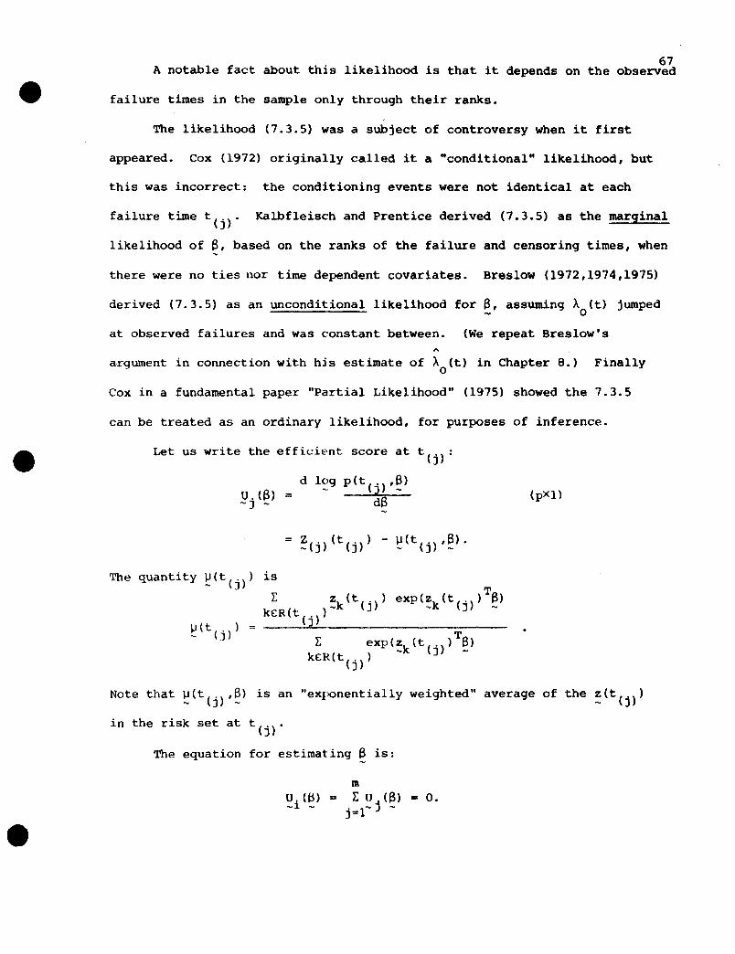
67A notable fact about this likelihood is that it depends on the observed
failure times in the sample only through their ranks.
The likelihood (7.3.5) was a subject of controversy when it first
appeared. Cox (1972) originally called it a "conditional" likelihood, but
this was incorrect: the conditioning events were not identical at each
failure time t(j). Kalbfleisch and Prentice derived (7.3.5) as the marginal
likelihood of a, based on the ranks of the failure and censoring times, when
there were no ties nor time dependent covariates. Breslow (1972,1974,1975)
derived (7.3.5) as an unconditional likelihood for a, assuming A (t) jumped- 0
at observed failures and was constant between. (We repeat Breslow's
argument in connection with his estimate of A (t) in Chapter 8.) Finallyo
Cox in a fundamental paper "Partial Likelihood" (1975) showed the 7.3.5
can be treated as an ordinary likelihood, for purposes of inference.
(pX})dau. (a) =-J -
Let us write the efficient score at t(j) :
d log p (t ( . ) , a)J -
Note that ~(t(j) ,~) is an "exponentially weighted" average of the ~(t(j»
in the risk set at t(j).
The equation for estimating a is:

A
Or, by writing a , for the solution, we define B by the equation-n -n
m
68
(7.3.9) E lz(.)(t(.» - \J(t(j),a)] '" o.j=l - J J - -n
A solution to (7.3.9) may not exist, as discussed in the next section.
The observed pxp information matrix is
(7.3.10)
where
m1(13) = r ~(t(.),~),
j=l J
That is, C(t(.) ,B) is the variance-covariance matrix of the z's in the risk- J -
set at t(j)' under the scheme of exponentially weighted sampling.
In the 1975 paper, Cox shows that under a wide variety of censoring
schemes,
(7.3.12)
E(~j(~» = 0 and v~r(~j(~» = -E(~(t(j) ,~» =
I (6) = lim(~ Ei.).-avg - n~ n -J
i. ,-J
say. Write
The sum rio has m terms; the divisor n is needed for work with F. If-J n
m/n ~ Q, say, then I (B) = Q(lim! rij). Under regularity conditions,
-avg - m~ m --1/2
a C.L.T. for dependent R.V. 's applies to n Eu. (B), and-J
(7.3.13)
12" A L
n (a -B) -+ N(o,l (a».-n - - -avg -
I (B) will be consistently estimated by-avg -
(7.3.14)
providing for large sample inference.

We can,
(7.3.15)
therefore, base large sample inference on the fact that1
1(6 )2 (6 -6) i N(O,I x ).- n -n - - -p p
69
7.4. Solvability of the Likelihood Equations
In this section, we briefly outline some conditions under which the
estimating equations 7.3.9 have no finite solution. For simplicity, assume
the z's do not depend on time. Then the likelihood equation 7.3.9 is
(7.4.1)m
1: (~(j) - ~(t(j) ,~) = ~.j=l
There will be no finite solution if, for some coordinate of ~, say
the q-th, and for all B,
(7.4.2) z (j) > «) IJ (t(,),B), j::o: l, ... ,mq - - q ) -
with at least one strict inequality. In words, we require z for theq
Let us see how this can arise in practice.
observed failure at t(j) to be greater than (less than) or equal to the
exponentially weighted mean of the Zq'S in the risk set at t(j).
Suppose Z is a 0-1q
indicator of group membership. Then 7.4.2 will hold if all of the l's are
failed or censored before the first 0 fails. For, suppose the first
O-failure takes place at t(t). Then, Zq(l) ::0: Zq(2) ::0: ••• = Zq(t_l) = 1.
But the risk sets {R(t(j»: j = 1, ... ,t-l} all contain some O's. Therefore,
IJ (t(,),B) < 1, j = 1, •.. ,t-l, _00 < B < 00, precisely because IJ (t(,) ,B) isq ) - q ) -
an average of the Z. As a result,q
(7.4.3) j ::0: 1, ... , l-l.
But if there are no l's left in the risk set at t(l)' then
(7.4.4) z(,)-IJ(t(,),B) -o,t<j<m.q ) q ) -

70Together, 7.4.3 and 7.4.1 imply 7.4.2, and Cox's likelihood has no finite
solution in this case.
Note that if there are any l's left in the risk set at t(~), then
Zq(j) < ~q(t(j) ,~) for at least one j ~ ~ and for any B. The estimating
equations 7.4.1 may then have a finite solution, illustrating a peculiar
role of censoring.
With no censoring, condition 7.4.2 will hold in general if, for some
q, 1 2. q < p,
(7.4.5) Z >z > >zq(l) - q(2) - ... - q(n)'
with at least one strict inequality. (The direction of the inequalities
7.4.5 may of course be reversed.)
7.5. The Estimator as a von Mises functional
With time dependent z's F is again defined to be the distributionsn
with mass lin at (t. ,o.,z.), is i=l, ... ,n. Note that z. (t) is only defined1. 1. -1. 1.
if t.>t; otherwise we may set z. (t) = 0 if t.<t. Our strategy is to1.- 1. 1.
write sums in 7.3.7 and 7.3.9 over the whole sample and divide by n.
The statement "k£R(t)" about risk set measurement is converted to
= 1."
We begin by writing the exponentially weighted mean ~(t,B) as a
functional of F. Let e be a pXl vector. Thenn
(7.5.1) ~(t,EJ) =
1 n T- E I[t >t]z.(t) exp(z.(t) 8)n. 1 . J -J-J= J-
1 n T- E I[t >t]exp(z.(t) 8)n. l' -J-J= J-
The division of numerator and denominator by n has converted the sums
to averages over the sample.
redefining ~:
We make the dependence on F explicit byn

(7.5.2) ~(t,e,F ) =- - n
A(t,e,F )- - nB(t,e,F )
- n
71
where (letting y be a dummy for time) :
(7.5.3)
~d
(7.5.4)
F(y,z) is the marginal distribution of (y,z), and integration is
over [0,00) x Z where Z is the domain of the covariates.
Note that 7.5.3 is formally equivalent to
(7.5.5)
(7.5.6) = E {p(Y>tlz) z(t) exp(z(t)Te )}.z - _ - __
Here t is a fixed time point, while Y and z(t) are random quantities. We
must assume the existence of the expectation on the r.h.s. of 7.5.S to
avoid measurability problems. Similar remarks apply to 7.5.4 and other
expressions in this chapter.
There is a connection here with the work of Efron (1977) on the
efficiency of Cox's likelihood, Efron makes his calculations on the basis
of the fixed sample zl,z2""'z. The randomness in the risk sets R(t)- - -n
is in his work due only to censorship and failure of the sample items.
For example, let P. (t) be the probabiliey that sample item i is in R(t).~
Then Efron (c.f. his equation 3.18) works with quantities like the
following:

72E{E z. (t) e xp (z. (t) T8) }
i£R(t)-~ -1-
(7.5.7)
nE P. (t) z . (t) exp (z. (t) T8) •
i=l 1 -1 -1-
Now,
P.(t)z.(t)1 -1
the probability P. (t) is p(Y.>tlz.). Therefore each term1 1- -1
exp(z. (t)T8 ) summed in 7.5.7 can be identified with the-1 -
quantity whose expectation is taken in 7.5.6.
The approach of this chclpter explicitly recognizes the randomness
of the z's, while the approach of Efron does not. However, asymptotic
arguments with Efron's work require some sort of long run distribution for
the z's. Indeed, in the two sample problem presented by Efron as an
example (z. = 0 or z. = 1), the two samples are present in fixed propor-1 1
tions p and l-p.
Using 7.5.2 we can write the estimating equation 7.3.9 for S over-n
the whole sample and divide by n.
(7.5.8) .!u(B )n- -n
1 n "= - E 6. (z. (t.) - lJ(t.,B ,F » = o.
ni=l 1 -1 1 - 1 -n n
For an arbitrary distribution F, let us define a functional S(F)
implicitly by:
(7.5.9) ~(~(F) ,F) = I 6(~(t) - lJ(t,B(F) ,F» dF(t,6,z) = o.
Then by 7.5.5, Cox's estimator is a von Mises functional, with B-n
•
B(F ).n
oNote that existence and uniqueness of a solution to 7.5.9 are not
guaranteed. Nevertheless, we will continue to speak of "the" Cox estimator
defined by 7.5.9.

7.6. Fisher Consistency
Suppose now that the covariates z do not depend on time. Let the
73
observations x = (t,6,z) be from a random censorship model (Definition 3.2.1),
with failure time S from a P.H. distribution 7.1.1:
Label the resulting random censorship distribution Fa{t,6,~).
In this section we show that Cox's estimator is Fisher consistent
under the random censoring. The equation defining the estimator for
arbitrary F is 7.5.6:
(7.6.l) u(8(F) ,F) = f6{~ - l..I{t,8{F) ,F»dF(t,6,z) = O.
Fisher consistency will hold if U{~,F8) = 0, that is if:
(7.6.2)
Let us rewrite 7.6.2 as
00 00
(7.6.3) JhdF8(t , 1 , ~)o Z
making explicit the region of integration as Z x [0,00] and 6=1. We will
evaluate both sides of 7.6.3 and show them to be equal.
We assume enough regularity in the distribution of F8(t,1,~) so
that a density function (with respect to Lebesg4e and counting measures)
exists (3.2.2):
(7.6.4)
We also assume that ~f8(t,1,~) and ~(t,~,F8) f8(t,1,~) are integrable on
Z x [0,(0), so that Fubini's theorem may be invoked.

We begin by writing74
~(t,~,Fa)= ",,"'Y_
B(t,~,Fa)
and evaluating ~(t,~,Fa) and B(t,~,FB) .
By 7.5.3,
00
(7.6.5) = f fZ 0
TI )z exp(~ ~) dFa(y,z:y).[y~t - -- ...
By definition, we have
(7.6.6)
When 7.6.6 is substituted into 7.6.5, let us assume that the
resulting function is integrable. We apply Fubini's theorem, finding
00
~(t,~,FB) f~T k(~) [f f~(yl~)= exp(z 13) dy) dz
Z t
h TFS(tl~)(7.6.7) = exp(z S) k (z) dz,
Z
h T H(t Iz) GS(tl~)exp(z 13) k (z) dz.
Z
The last equation holds because
by the conditional independence of Sand C, given z, in the random censor-
ship model.
In a similar fashion, we can show
(7.6.9) B(t,~,FS) = Jexp(zTS) k(z) H(tl~)GB(tl~) dz.
Z

We now write the r.h.s. of 7.6.3 as 75
R.H.S.
(7.6.10)
using Fubini's theorem.
By 7.6.4, this is
00
IIA(t,a,Fe)
= : a dFa(t,l,z)B(t, ,Fa) -o Z - _ -
(7.6.11)
(7.6.12)
(7.6.13)
R.H.S.
00
[fga(tl~) H(tl~) k(z) d~)dt,Z -
lIAo(t) exP(~T~)G8(tl~) H(tl~) k(z)d~)dt,Z
(7.6.14) = I A(t,~,F~)AO(t)dt.o
We further evaluate 7.6.14 using 7.6.7
00
I I: TH(tl:) Ga(tl~) A (t)dz dt.R.H.S. = exp(z S) k(z)
o -o Z
00
= I J: ga(tl:) H(tl~) k(z)dt dz,
o Z
00
= I I~ dFa(t,l,:), by 7.6.4
o Z
= L.H.S. of 7.6.3.
This proves Fisher consistency. o

76Remark: The reader is invited to try a "proof" of Fisher consistency with
time dependent z's, along the lines of this section. Surprisingly, if.the
formal manipulations are carried out with Fubini's theorem--such a "proof"
will go through.
7.7. The Influence Curve
In this section, we derive the I.C. for Cox's estimator, allowing
the covariates to depend on time. The strategy for finding the I.C. is
similar to that in Chapter 6. We contaminate an arbitrary F with
* * *x = (~,o ,z ), the resulting distribution is F£ = (l-£)F + £ Ix.. The
Cox estimator based on F£ is defined by U(6(F ),F ) = 0 (7.5.6). This- - £ £ -
equation will be differentiated with respect to £ in order to find
:£ ~(F£) I ' the influence curve.£=0
Before we proceed, it will be helpful to restate the definitions of
some functionals needed in the sequel and to define some new functionals.
* • •To avoid confusion with the contaminating point (t ,0 ,~ ), let y and u
be variables for time.
From 7.5.2, 7.5.3, and 7.5.4, we have the exponentially weighted
mean at y:
where
l-/(y,n,F)
pXl
A(y,e,F)- -=B(y,e,F)
and
A(y,O,F) = II[U~]~(Y) exp(~(y)T~) dF(u,z)
pXl
B(y,e,F) = fl[U~] exp(z(y)Te ) dF(u,z).

Define the matrix D(y,e,F) by- - -77
(7.7.1)
Then let
(7.7.2) C(y,e,F)D(y,e,F)
= - - - ~(y,e,F)B(y,e,F)-T
~(y,e,F) .
The reader may verify that C(y,e,F ) is just the exponentially weighted- - n
covariance matrix of the z's at y, defined at 7.3.11.
Finally let
1 (e,F) = Jo~(y,~,F) dF(y,O)-avg ---
pxp(7.7.3)
~ J~(Y'~'F) dF(Y,l)
Note that I (O,F) is analogous to the average information matrix-avg
I (6) defined at 7.3.12. The relationship will be discussed in 7.8.-ilVg
To ease the notational burden, we adopt the convention
(7.7.4)
Then
13(0) = 13(F).
The defining equation for 13(£) is
(7.7.5) u (13 (£) , F ) = Jo (~ (y) - ~ (y , 13 (£) , F ») dF = O.- - £- - - £ £
The I.C. will be
Wo now expand 7.7.5.

(7.7.6)
* *. *+ £ 0 (z (t ) - )..I (t , S (£) , F » = O.- £
Or
* * * *o = (1-£) U(S(£) ,F) + £ [0 (z (t ) - lJ(t ,6(£),F »1.- - £
We now differentiate 7.7.6 coordinate by coordinate with respect to £
and evaluate at £=0.
78
(7.7.7)
o ~c ~(~(£) ,F f ) I = ic u(6(£) ,1") I£=0 £ - £=0
* * * *+ 6 (z (t ) - pet ,~(O) ,F)}- U(S(O) ,F)
d * • *;)E ~(s(n,F)lc'=o + 0 (z (t)
*)..I (t ,6 (0) , F»,- -because u(S(O) ,F) = 0 by 7.5.6.
Now
aa£ ~(~(£) ,F) I
£=0
(7.7.8)
= ~ I(z (y) - )..I (y , S(£) , F ») dF (y , 1) Io£ - - - £ £=0
We assume sufficient regularity in 7.7.8 to allow differentiation under
the integral sign. Sufficient conditions are given, fOr example, in
Theorem l7.3e of Fulks (1409). Assume:
a. I)..I(y,(3(C),F) dF(y,l) and f~ )..I(y,S(E),F ) dF(y,l)- - C a£ - - £
are continuous with respect to y and £.
b. There is an £' fOL which IJ..I(y,6«('),F ,) dF(y,l) converges- - e:
(true here for £' =0) •

c. I~ V(y,B(£),F ) dF(y,l) converges uniformly for 0<£<1.a£ _ - £
With these assumptions,
79
(7.7.9)
The inner derivative is:
(7.7.10)
(7.7.11)
We require
dId ~~(Y'~(E)'FE)~d£ ~(y,~(£) ,FE) E=O = a£ B(y,a(E),F )
- E E=O
= {S(y, ~ (0) ,F) [iE ~(y) ~ (E) ,FE} IE=O]
- A(y,I3(O) ,F) [~ B(y,I3(£),F) I -olL 1 J- - a£ - E £- ~2(Y,I3(0)'F;I
~ A (y , B(£) , F ) I and ~ B (Y, 13 (£) , F ) I .a£ - - £ 0 a£ - £ 0c= E=
We find the first of these expressions by writing out ~(y,~(E),FE):
(7.7.12) = A(y,B(£),F)
Here
Texp(z(y) B(E» dF (u,z)
- - I:
[* * To+ £ I[t*~l~ (y) exp(z (y) ~(c»
- ~(y,~(E) ,F}l(7.7.13)
Then, differentiating 7.7.12,
(7.7.14)
* * Tn+ I I t *> ) Z ( y) e xp ( Z (y) ~ (0» - A(t , l3 (0) , F) .-Y

The first term of 7.7.14 is
a . ,a£ ~(y,~(£) ,F) £=0
80
(7.7.15)
~(y) exp(~(y)T~(£) dF(U,Z)ll •J £",,0
Again let us assume that we can differentiate with respect to £
under the integral sign in 7.7.15. (Recall that the regularity conditions
in Theorem 17.3e of Fulks (1969) will apply only when z does not depend on
time.) They by the chain rule of multivariable calculus, we have
(7.7.16)
(pXl)
J1 [u~yl ~ (y) [~£ exp (~(y)T ~ (£)) 1£=0] dF (u, Z)
J1 [u~yl ~ (y) ~ (yl T exp(~ (y) T~ (0)) [:£ ~ (£1 1£=0]dF (u,~)
= D(y,(3(O) ,F) (3' (0),-pxp- pXl
where D(y,(3(O) ,F) was defined at 7.7.1. Note that (3' (0) is the influence
curve we are seeking.
Therefore, collecting terms from 7.7.16 and 7.7.14, we have
~ A(y,13(£),F) I 0oC - 1 E E=px
• • TD(y,S(O) ,F) 13' (0) + I[t.5)~ (y) exp(z (y) (3(0»
pxp pXl pXl
- A(y,(3(O),F).-pxl-

In a similar fashion, we can find:
()"B(y,B(£),F );aE: - £
81
(7.7.18)
paralleling 7.7.12 - 7.7.14.
The first term on the r.h.s. of 7.7.18 is
()aE B(Y,~(£) ,F) I
£=0
-~ II exp(~(y) T~(£» dF(U,~) I- ()£ [U51 £=0
(7.7.19)
TA(y,B(O),F) p'(O)
lXp pXl
assuming we can differentiate under the integral sign. Again 13'(0) is the
I.e.
Therefore
~£ B(y,~(E:) ,F£) I = ~(y,~(O) ,F) T ~'(O)£=0
(7.7.20)
* T+ I(t*51 exp(~ (y) 13(0» - B(Y,~(O) ,F).
We ndw simplify notation by writing

(7.7.21)
We also write
82A(y) = ~(y,~(O),F)
pXl
B(y) = B(y,~(O),F)
~(y)
l.I(y) = B(yfpXl
~(y) = ~(y,~(O),F)
pxp
~(y) = ~(y,~(O),F).
pXp
tHo) = B,- -suppressing the dependence on F.
We now substitute from 7.7.20 and 7.7.17 into 7.7.11:
* * T= [B(y)~(y)~' (0) + B(Y)I[t*51~ (y) exp(~ (y) ~) - B(y)A(y)
(7.7.22)T
- ~(y)~(y) ~'(O) - ~(y) I [t*511
+ ~(Y)B(Y)l [B2(y)1
~)(y) A(y)A(y) TJ--- - - - a' (0)B(y) B(y)B(y) -
* Texp(z (y) a)- -
(7.7.23)
( *( )TD ) ~z*(y) A(y)]+ I * exp z y ~ - - -[t ~y) - - B(y) BZ (y)
This result is substituted into 7.7.8.

~£ ~(~(£) ,F) I ..,£=0
(7.7.25)
00
-[I~(y) dF(y,l»)~'(O)o
00
83
(7.7.26)
- II[t*~]exP(~*(y)T~) (~*(Y)-~(Y»dF(y,l)o B(y)
t*
= -I (6,F)6' (0) - IexP~(Y)'_)(Z_*(Y)-ll_(Y»dF(Y,l).-avg - - _~
o B(y)
(7.7.27)
We substitute 7.7.26 in turn back into 7.7.7:
t*
0=-1 (6,F)6' (0) - IexP(~*(y)T~) (z_*(Y)-ll_(y»dF(y,l)-avg - - --~
o B(y)
We can now solve for 6'(0) *= IC(x iB,F).
The result is a
Theorem 7.7.1
Let Cox's estimator 6(F) be defined by 7.5.6, and let I (6(F) ,F)-l-avg -
be an inverse of I (6(F) ,F). (A generalized inverse will do.) Then-avg -
the influence curve for Cox's estimator at x* • (t*,o*,z*) is...
* * *le( (t ,6 ,z ) i6,F)
The empirical• O.
!avg(~(F) 'F)-l{-I::PI~*IYlT~(Flll~*(Y)-~(YlldF(Y'l)o B(y)
+ 6* (~* (t*)-~(t*))} .
*shown that EF(~C(x J~,F)In Appendix A2 it is
I.e. and robustness are discussed in 7.9.

7.8. The Squared I.C. Under Random Censorship
According to the theory of von Mises derivatives, we expect
84
(7.8.1)
where
(7.8.2)
~(8 -6) ~ N(O,V(F»-n .~
(7.8.3)
Suppose now that the P.H. model holds in the random censorship
setup of Section 7.6. (In that setup, recall that the covariates do not
depend on time.) As in 7.6, call the resulting distribution Fa.
The main result of this section is Theorem 7.8.1, which states:
T -1E
FS(~C(x;~,FB) ~C(x;~,FB) ) = !aVg(~,Fa) .
~lThis implies V(Fo ) = 1 (a,Fa )
- I.J avg - I.J
How does this compare to the asymptotic covariance matrix from
Cox's (1975) partial likelihood? That theory, as quoted in 7.3, gave a
-1covariance matrix of 1 (B) ,where 1 (a) was defined at 7.3.12.
-avg - -avg -
Writing 7.3.12 in functional form, we see that
(7.8.4)
1 (a)-avg -
n= lim{-E (~ E C.C(t. ,a,F )}
Fo n . 1 1_ 1 - nn-)(lO I.J 1=
The identity of 1 (8) ,md 1 (13, Fa) should follow from the mild-avg - -avg - I.J
conditions of Cox's theory; but no proof will be given.
We begin the proof of the theorem with two closely related lemmas.
These were implicitly proved in Section 7.6. Lemma 7.8.1 will be of
use in Chapter 8.

Assume the P.H. model 7.1.1 for failure time:
with a random censorship distribution as in Section 7.6. With the
integrability conditions of Section 7.6, then
85
LeIlll\a 7. 8 •1.
Lemma 7.8.2.
Proofs:
By 7.6.4 and 7.2.5
(7.8.5)
Then
dFS(t,l) = IdFS(t,l,:)
z(7.8.6)
by 7.6.9. This proves Lemma 7.8.1.
Also,
dFB(t,ll:) = dFS(t,l,:)
k(z)dz
(7.8.7)
by 7.6.8, proving the second lemma.
Theorem 7.8.1. With the assumptions of the previous lemmas
o
(7.8.8)-1= I (a,Fa )
-avg - ....

Proof:86
(7.8.9)
Then,
-1I (13,FQ ) {-w(t,z) + O(z-ll{t» },say.-avg - p --
pxp pX1 pX1
+ O{z-ll(t»}
T20w(t,z) (z-ll{t»
(7.8.10)T -1
+ 6{Z-1l(t» (z-ll{t»}I (B,FQ )
-avg - .....
where
N(t,O,z)
TM(t,z) =, w(t,z) w{t,z)
and
(7.8.11)
Then
pxp
N(t,6,z)
pXp
lXp
T26w(t,z)(z-P(t» .
lXp
(7.!:L12)
TE
FS(I_C«t,6,:) ;~,FS) I_C{(t,O,:) ;~,FB) )
1 (B,FS)-l{B (M(t,z) - N{t,z»}I (B,FS)-1-avg - F
B- -avg -
-1 T-1+ !avg(~,FB) tEF(O{:-~{t» (:-~(t) )}!avg{~,FB)

We compll,te the proof in two parts. In Part I, we show that
E (M(t,z) - N(t,6,z» = O. In the second part, we show thatFa - -
E {O(z-~(t» (z_~(t»T} = I (a,Fa ). The theorem follows immediately.Fa - - - - -avg - ~
Part I.
87
To show: EF
(M(t,z) - N(t,O,z» m O.a - - - - -The following step is crucial. Define the pXp matrix
where the differentiation is coordinate by coordinate. Then
(7.8.13)
Comparing ~l(t,~) to ~(t,6,~) defined at 7.8.10, we see that
(7.8.14) N(t,6,z) = 6~1 (t,~)B(t)
exp(~T~) ~Fa~:'1)J
By Lemma 7.8.1, this is
(7.8.15)
Then
N(t,6,z) = 6~1 (t,~)
exp(zTa)A (t)- - 0
00
(7.8.16)
E (N(t,6,z»Fe - f f ~1 (t,~)dFa(t,1,:)Z 0 T
exp(z a)A (t)- - 0

88
00
by Lemma 7.8.2.
We also evaluate E (M(t,z»:Fe - -
(7.8.17)
-J r~(t.~)dFa(t'~))dK(~).Z 0
Therefore
E (M(t,z) - N(t,O,z»Fa - - - -(7.8.18) f~ro
- (~(t,~)dFB(tl~)
Z dt
The elementary rUle for differentiation of products reveals
(7.B.l9)
Let us clSSumC that for ('very z, the elements of the matrix H(OO,z)
are finite. This will be tnl(' it. fer inslancp, the cov.:lriates ore bounded.
Or, more realistically, the a~;sumption will hold if there is an upper
limit of observation,C , so that H(C Iz) = o.max max -
With the assumption, ~he inner integral in 7.8.18 can be evaluated
by the fundamental theorem of calculus and 7.8.19:

00
= f ~t ~(t,~) FB(tl~)dto
= M(oo,z) x 0 - 0 x 1
= o.
Therefore, the entire integral 7.8.18 is zero, and
EF
(M(t,z) - N(t,6,z» = o.B - -
Part II.
We must show that
89
(7.8.20)T
Ep (6(z-~(t» (z-~(t» ) l% J (B,I"o).B -avg - I-'
It is ea~;ier to start flom the r.h.s, defined at 7.7.3:
00
I (B,Fo )-avg - I-'
f ~(t,~,Fa) dFa(t,l).
o
Recall from the remark at 7.7.2 that ~(t,~,FB) is the exponentially
weighted covariance matrix of the z's in R(t); we can, therefore, write
it as:
00
And, assuming we can apply Fubini's Theorem:
1 (B,Fa )-avg - I-'
" I~[IImexP(~T~)(c-~(t» (~_~(t»T dFa(yl~) k(~)d~]dFB(t'l)o -Zt B(t)
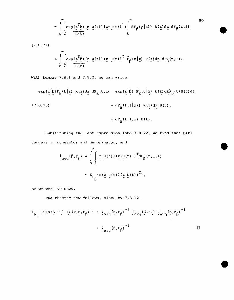
00
= I JeXP(~T~) (~-~(t)) (~-~(t»T(I dFa(y\Z» k(~)d~ dFa(t,1)
o Z -8ft) t
(7.8.22)
on
J JexP(:T~) (~-~(t) (:_~(t»T Fa(tl:) k(z)dz dFa(t,l).
o Z B(t)
With Lemmas 7.8.1 and 7.8.2, we can write
90
(7.8.23) = dFa(t,1Iz» k(z)dz B(t).
= dF8 (t , 1 , z) B ( t) .
Substituting the last expression into 7.8.22, we find that B(t)
cancels in numerator and denominator, and
00
I (S,Fa )-avg - IJ
as we were to show.
JJ(~-~(t» (~-~(t) ) TdFS (t,l,~)() Z
TE (O(z-v(t»(z-V(t»),
FS - - - -
The theorem now follows, since by 7.8.12,
'I'EI-' l (~'(x;~,l"l;) l~C(xd~,F(:)) )
bI (R,F )-1 I (B,p) I (S,F )-1-avq - B -~vg - B -avg - B
[J
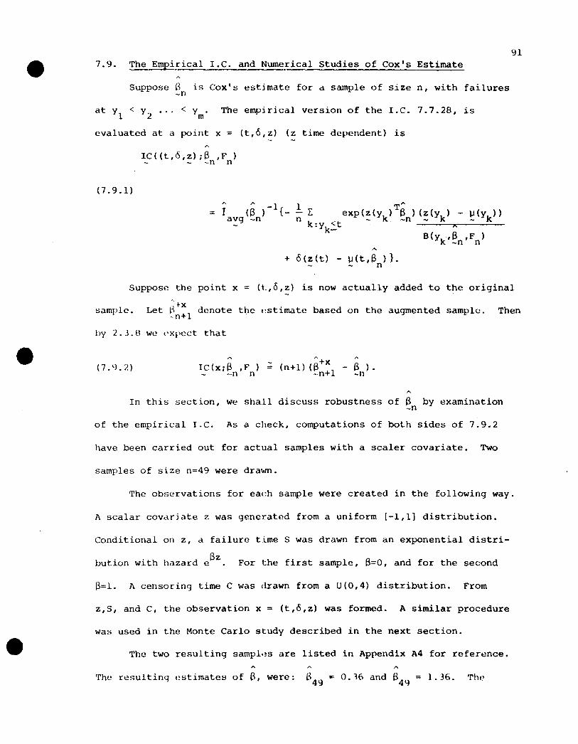
917.9. The Empirical I.C. and Numerical Studies of Cox's Estimate
Suppose B is Cox's estimate for a sample of size n, with failures~n
at Yl
< Y2
•.. < Ym
' The empirical version of the I.C. 7.7.28, is
evaluated at a point x = (t,6,z) (z time dependent) is
IC( (t,6,z);l3 ,F )- - ~·n n
(7.9.1)
+ 6(z(t) - ll(t,S )}.- n
Suppose the point x = (L,6,~) is now actually added to the original
sample. Let ~~~=l denote the t!stimate based on the augmented sample. Then
by 2.3.8 we t'xpect that
(7.9.2) IC(xd3 ,F )~n n
- "+x= (n+1) (B 1 - 8 ).-n+ -n
In this section, we shall discuss robustness of 8 by examination~n
of the empirical I.C. As a check, computations of both sides of 7.9.2
have been carried out for actual samples with a scaler covariate. Two
samples of size n=49 were drawn.
The observations for each sample were created in the following way.
A scalar covariate z was gener.ated from a uniform [-I,ll distribution.
Conditional on z, a failure time S was drawn from an exponential distri-
Bzbution with hazard e • For the first sample, 8=0, and for the second
13=1. A censoring time C was drawn from a U(0,4) distribution. From
z,S, and C, the observation x = (t,6,z) was formed. A similar procedure
was used in the Monte Carlo study described in the next section.
The two resul ting sampl.~s are listed in Appendix A4 for reference.
The resulting estimates of S, were: 849
'" 0.36 and 84q = 1.36. The>
first sample thus provides a "small" estimated B and the second a "large"
one, as desired.
We begin our examination of ehe empirical I.C. by observing that it
is the sum of two parts, both multiplied by I (6 )-1. The first part-avg -n
is
The second part is
In the augmented sample, the added observation is present in those
risk sets R(k)' such that Yk~t. This presence is represented by Ql "
On the other hand, Q2
can contribute to the I.C. only if the
added observation is a failurl! (~=l). In this case a new risk set at t
is formed. This may not be aile of the original m risk sets. As a con-
vention, we agree that if t is larger than all n sample times, then
~(t,S ) = z(t)" In this case there is therefore no contribution from Q2'- n
Indeed in the ~lUgmented sample, with t the largest observation, we must
have
since only z is in R(t}" Ref(~rence to th!' original likelihood equations
(7.3.9) shows that the contribution of x then does not depend on 8.
92
We now consider in detail how an observation x = (t,8,z) influences
S To do so, it seems useful to consider two cases separately. In the-n
first, we assume z and 6 are fixed, but t moves. In the second case t
and 6 are held constant, but z is allowed to vary.

For t>y , Ql(t,z) is constant.m -
93
Case 1: Fix z and 6~ vary t.
For fixed z = {z(y) :y~O}, the term Ql(t,~) is a step function in t,
taking on m+l possible values. For t<yl
, Ql
(t,z) = O. A term is added
to the sum for each failure Yk
with Yk2t.
Ql
is therefore bounded.
The term Q2(t,6,~) is also bounded. For time dependent zls, z(t)
and ~(t'~n) may vary continuously with t. Therefore Q2 is not, in
general, limited to a finite number of values, as Ql
is. For zls which
are not time dependent, Q2
takes on at most n+l values; there is a value
for each original observation t., i = l, •.. ,n, and zero, as agreed, for1
t>t , the largest sample valu(!.n
From these observations we may conclude that the I.C. is discon-
tinuous as a function of t and is bounded. The same conclusions should
apply to the quantity 50 (B;~ - 649 ). Let us turn to the sample data to
check these conclusions.
For the first sample, B49
= 0.36. The largest observation was a
failure at t == 3.69. In Figure 9.2.1 the Ic(t,6,z) is plotted for the
four combinations resulting from z = {-l,+l} and 6 = {O,l}. Thus the
curve labeled "1" is the combination (z == -1,6=0); the curve labeled "2"
is (z = -1,0=1) and so on. The horizontal axis is plotted from t=O to
t==4.
. . d' f r. ( ~+x Q )The correspond1ng norma]1zed 1f erences are :>0 1->50 - 1->49' These
are designated "DIFF" and are plotted in Figure 7.9.2. The I.C. and
DIFF were plotted and were both calculated at increments of 0.10 in t.
We can see that the I.e. plots are very similar in shape to the
corresponding DIFF plots. Thl' I.C. exaggerates the true influence at
values of t. Both the I.C. and DIFF curves are discontinuous in t, as

94predicted. 'fhe curves are geJlPrill I y monotone, except for a few
instances.
The curves at z=+l decroase with increasing t. This is to be
expected. As t increases, we expect the estimated hazard to decrease."8 "
For z = +1, this hazard is e ; therefore a should increase. Also at z = +1,
an added failure (0=1) should result in a larger estimated hazard than an
added censored time (0=0), no matter what the value of tis.
precisely the behavior shown by the I.C. and DIFF.
This is
For z = -1, the estimated hazard is e8. By symmetry we can account
for the increase in a with increasing t. For either value of z(-l or +1),
the value of l) does not affect the estimate of t > 3.69, the maximum
sample observation. In this sample, the largest change is 850
occurs
in the case (z=l,O=l). The re-estimated values of s+x range from 0.4250
at t=O to 0.11 for t = 3.69.
Now let us turn to the second sample, which resulted in 849
= 1.36.
In this sample, the maximum observation was a censoring time at t = 3.99.
The four empirical influence curves for z = {-l,+l} and 0 == {O,l} are
plotted in Figure 7.9.3. The DIFF curves for the normalized change in aare plotted in Figure 7.9.4.
Again the I.e. curves strongly mimic the shape of the DIFF curves.
But the influence curve also badly overestimates the large changes in the
estimator for z +1. The discontinuous effect of the risk sets is also
apparent here. Indeed, of 27 failures, only two occurred after t = 1.5.
The curves for z = +1 show much more of a change with t than do the
curves for z = -1. The original data give, for z = +1, an estimated mean
failure time of E(S) = ;1.36 = 0.25. Larger observed times dramatically
decrease the estimate (from 850
= 1.42 at t=O.O and 0=1 to 850
= 0.95
for t == 4.0 and 0=1).

95From these examples, we may conclude that the influence of t on B
n
is indeed bounded. A virtue of the Cox estimator is that only the ranks
and not the values of t enter into the estimate. Therefore any monotone
transformation of the original sample times leaves the values of the I.C.
unchanged. The most that an outlier can do is shift from being largest
observation to smallest. The actual value does not matter.
The discontinuities in the I.C. and normalized difference curves
have been noted. These discontinuities mean that B is sensitive to local
shifts in the data--the "wiggling" mentioned in Section 2.3.
Case 2: Fix t and 6; vary z.
We have seen that the I.C. and normalized change in the estimate are
both bounded, as functions of t. As a function of z, the I.C. is con-
tinuous and unbounded. There are terms linear in z and also there are
exponential terms: If the actual change (S+x - S )-n+l -n
depends exponentially on z, this would pose a serious problem. For
outliers in z could potentially cause large changes in S. This phe-
nomenon of "influence" of position of the independent variables was
encountered in the cases of multiple least squares regression
(Section 2.3) and of exponential survival regression (Chapter Six).
It is therefore of interest to look at some examples.
"'+x '"Plots of the I.C. and of DIFF ; (n+l) (8
n+
l- 5
n), as functions of
z, were made from the two samples of n :c 49 described earlier. Four
combinations of (t,6) were considered. In each, z ranges from -5 to +5
in increments of 0.2; recall that in the original samples z is in the
interval [-I,ll. The four combinations of (t,6) are: (1) t=0,6=1;
(2) t=1,6=0; (3) t=1,6=l; and (4) t=4. By our earlier discussion, the
curves for t=4 will be the same for 6=0 and for 6=1. Also, an added
point with t=O and 6=0 has no influence on the estimate. Therefore the

96points chosen cover the range of possible (t,O) values.
For the first sample (S = 0.36) the I.C. 's are plotted in
Figure 7.9.5 and the corresponding OIFF curves are plotted in Figure 7.9.6.
For the I.C. all curves except that at t=O show the effect of the exponen
tial term. Indeed the curve at t = 4.0 has a value of -401.0 at z=5.
When we turn to the actual OIPF plots, we notice that the predicted
exponential declines in ~ do rIot take place in the curves 2, 3, and 4.
These curves seem to level off as z becomes larger; indeed thi.s is true
of curve 1 also.
Nonetheless, the I.C. mimics the qualitative behavior of all four
DIFF curves. For example, both curves for situation 1 are approximately
linear. It is interesting th.lt the DIFF curves are not necessarily
monotone in z, for curves 2,~, and 4. The I.C. captures this behavior,
at least for curves 3 and 4.
Plots of the I.C. 's from the second sample (S = 1.36) are shown in
Figure 7.9.7. Withthe larger value of S, the exponential fall-off in
curves 2, 3, and 4 is more pr'Jcipitous than before. The corresponding
DIFF curves aro plotted in Fi'Jure 7.9.H. Again the actual fall-off in
650
is not nearly so severe a~ the I.C. 's predict.
The I. C. therefore has ,~xaggerated in both samples the extreme
effects of outliers in z. But comparison of the I.C. and DIFF curves
show close agreement for smaller values of z. And, in both samples, the
changes in 650
caused by outliers in z are more extreme than the changes
caused by the variation in t.
Remarks
We close this section with a few miscellaneous remarks on the I.C.
A small Monte Carlo simulation is presented in Section 7.10. Conclusions
and recommendations will be made in Section 7.11.

e - e
Fig. 7.9.1. Plots of the empirical influence curve for Cox's estimate against t: n=49, B =0.36.n
The cases are: 1: (z=-l,C=O) 2: (z=-l,C=l) 3: (z=l,C=O) 4: (z=l,O=l).
"~1'I
", .. ,.
3 3 3 3 3 3 3 3 3 !
1 1 111 1 1 1 1 1
2222222 222
4 .. • II II
3 3
1 1
222 2
II •
3 3 3 3
444411
""'1'
4
3 3 3 33 J 3
1 1 , 1
333
1 1 1
8 +--------------------------------------------------------------------------------1I l-~11I,,
II ~
,. II, 'Q 4, 411111t 1111 Illlll
o ~~1-------------------1l-.-----------------2-2----------------_A- .._~_., ~ ~ ~ ~ , 222 222f 3 2222114'2, 2 2 2 2, 222 JJ
-4 ~ 2 2,2Ie I,
I-8 ..
III,
-12 ~,,I,
-16 ..IfI,
-20 +,,I,
-2/1 +-+-------------------+-------------------f-------------------+-------------------+o , 2 3 ,
'!'\£l....a

Fig. 7.9.2. Plots of the normalized difference in Cox estimates against t: n=49, 8 =0.36._ n -The cases are: 1: (z=-l,~=O) 2: (z=-l,O=l) 3: (z=l,O=O) 4: (z=l,O=l).
8 +--------------------------------------------------------------------------------1I 1, I1 1 1 ~ 1I 1111111111 I
Q + 1""'2222222222 I'QQ 1111111 I1 Q Q II 1 , I'Q111111 2222 I1 "" QQQll 22 I
o +'-1-------------------Q-Q-------------------------------------------------------I 313 3 4 2 222 2 2 2I 3 222 2 Q II III 2 2 2 2122 2 333 Q Q 0 • Q 0
-0 +2 2 2 3 3 Q Q
1 333 OQDIY!' , 3.Q Q
1 3333333 'lala'laltlt1
-8 + J JI,II
-'2 +I!,I
-16 +IIII
-20 +II,I
-2Q +
3 3 J 3 3 3 3 3 J J
3 3 J 3,II
e
-+-------------------+-------------------+------------~-----+--------------.----+o 1 2 J •
T
e e
..0IJ:)

e - e
Fig. 7.9.3. Plots of the empirical influence curve for Cox's estimate against t: n=49, 8 =1.36.nThe cases are: 1: (z=-1,8=O) 2: (z=-l,o=l) 3: (z=l),O=O) 4: (z=l,O=l).
8 +----------------~---------------------------------------------------.. ---------,II
11111111111
IIIII /I
1 11/1 """"",",,',,11111,o +1-'- '-1-'-1-----------~------------2-2-2-2-2-2-2-2-2-2-2-2-2-2- 2-2-2-2-2-2-2-2-
I 3 '3 II133 II II /II 3 2 2I 3 3
-8 + 2 2 2 2 2 2 2 3 312,I,
-'6 +I
Ie III
-2' +t1II
-32 +IIII
-flO +IIII-/18 +IIII
-56 +
2 2/I 2 2222 2
II II II .. •3
/I ..333
3 3
, II .. .... .. .. II II .. ..~ 3 II
3 3 3 J J 3 J J 3 333
II , II .. II , , II , •
IIII
3 3 3 3 3 3 3 3 3 3 3III
-+-------------------+-------------------+-------------------+-------~---------+o 1 23'
'1'
\0\0

Fig. 7.9.4.
e
Plots of the normalized difference in Cox estimates against t: n=49, 6 =1.36.The cases are: 1: (z=-l,o=O) 2: (z=-l,O=l) 3: (z=l,O=O) 4: (z=l,O=l). n
8 +--------------------------------------------------------------------------------1I 11 I,~ " II ~~ 11111111111111111111111111111111111
o +1-1-1-1-1-1-------------------------2-2-2-2-2-2-2-2-2-2-2-2-2-2-2-2-2-2-2-2-2-2-1I 3 4 2 2133 4 4 ~ ~ 2 2133 222 222I 2222 ~ll
-8 +2 2 2 2 3 3 3 ~ III 3 3 31 3 3 III 33 llllllllllllllll'll'I
-16 + 3 3 3 3 3 3 3 3 3 3 3 3, a .. 411 ••••••
DIP!' ,1333 3 333 3 3 3 3
I-2'1 +
IIJ,
-32 +II,I
-'0 +I,I1
-II" +"11tI
-56 +-+-------------------~-------------------+-------------------+-------------------+o , 2 3 •
T
- e
Ioo

e
:ig. 7.9.5.
-Plots of the empirical influence curve for Cox's estimate against z:The cases are: 1: (t=:J,C=l) 2: (t=l,O=O) 3: (t=1,5=1) 4: (t=4).
....n=49, 13 =0.36.
n
e
20 +----------------------------------------------------------------------------------------------------11 1I 1 1111
, 1I 1 1I 411444444 1IIIIIIIQQ IaQQ 11
10 +" " 1 1I II 1I 4 " 1 1I 1 1, '"1 '" 112 2 2 2 2 2 2 2 2 2 2 2 2 2 2 2 2 2 2 2 2 1I 2222 113
J... 3311 3333I 331 22 3, 33" 4 2 33, 33 1 22 3
IC I 3 3 1 1 2I 3 3 1 , Il 2 3t 3 1 3t 3 3 1 1 2
-1:> + 3 3 1 1 "2 3I 3 1 2I 3 3 1 1 3I 3 1 II 2I 3 3 1 1 3I 3 1 1 2J 3 1 "3I 1 1 2
-20 +'I 2 3I •I, 2 3II 2I II
-30 + 3-+---------+---------+---------+---------+---------f---------+---------+---------t---------+---------+-~ -II -3 -2 -1 0 1 2 3 II 5
7:
to-'oto-'
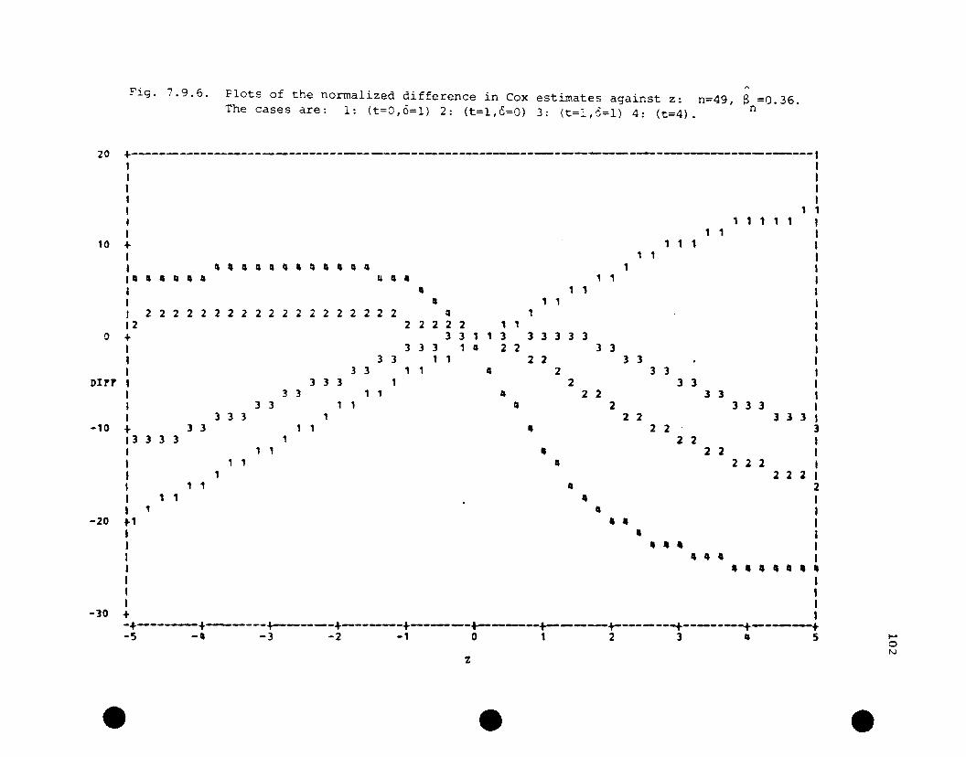
Fig. 7.9.6. Plots of the normalized difference in Cox estimates against z: n=49, 8 =0.36." ;:, nThe cases are: 1: (t=O,O=l) 2: (t=l,u=O) 3: (t=l,::'=l) 4: (t=4).
20 +----------------------------------------------------------------------------------------------------1I I, II II I111
I 1"'1, , ,10 + , 1 1
I 1 1,llllllllllllllllllllllQ 11""1111111& UQ. l'I "1,, II 1 1I 222 2 2 222 2 2 2 2 2 2 2 2 222 II 112 22222 11
0+ 3311333333, 333 '11 22 33I 33" 22 33, 3 3 1 1 " 2 3 3
DUr I 3 3 3' 2 3 3, 33 l' Il 22 33I 33" "2 333, 333 1 22 333
-10 + 3 3 1 , II 2 2 313333 1 22 I", II 22 I," "222 I1 1 2221, 1 1 "2I 1 1 Il 1I 1 "I
-20 +1 II II II Il II II II II 1
I '''' 1Ill." Il " • "
I I, I, I
-30 + I-f----f------+--------f-----f---------+------+----f--------+--------f----f-5 -" -3 -2 -1 0 1 2 3 Q S
e
z
- e
....or-J

e
Fig. 7.9.7.
e
Plots of the empirical influence curve for Cox's estimate against z:The cases are: 1: (t=O,6=1) 2: (t=1,6=O) 3: (t=1,6=1) 4: (t=4).
,..n=49, 8 =1. 36.
n
e
3 J3 1
3 3 1 13 1 1
3 3 13 1 1
331 13 1
331 13 3 1 1
3 1:3 3 1 11 1
1 11 1
1, 1
1 122:3 :3 3 1332113
1 1 2 31 2..
2 3
It2
3
•2
:3
•2
....ow

Fig. 7.9.8. Plots of the normalized difference in Cox estimates against z: n=49, 8 =1.36.The cases are: 1: (t=O,O=l) 2: (t=l,O=O) 3: (t=1,5=1) 4: (t=4). n
16 +----------------------------------------------------------------------------------------------------1
I-'o.s:o
1 11 1 1 1
1 1 111'11 1
2 3
2 3
1 1 1
3
2 3
2 3
,
2
3
•
2
4
3
1 ,
2
Ia
/I"1 1
J 3
1 1J
3 31 13 3
1 ,3
3 31 ,3 3
, 13 33 ."
3 3 1 13 3 1 1
1
• • 4/1/1 2 2 222 2 2 3 J 3 12 2 2 2 2 2 2 2 222 2 2 2 2 222 332 1 1 3
3 3 1 1 2, u
8
II,+1I1
o +2I,J
-8 +I,I+IJJ+J 3 3II 1 1,1 1+ 2 3J .),I 2 3 II • 2 J+ 2 3 I• /I 3 II • 2 3 3 ,I 2 2 3 I+ 4 2 33 II 4 2 3 IJ 114 22 333I II 2 2 I+ /I /I 2 21 /I /I II /I 4 II II 4 /I+ 1-+------+-------+---+-----+---------+-----+-- - +------+--------+--- -- -+-S -4 -3 -2 -1 0 1 2 3 /I 5
01""
-laS
-2'
-16
-32
-40
-56
-64
z
e e e

One cause of this complexity is multiplication
1051. The discussion in this section has been mainly in terms of a scalar
covariate. The sensitivity of Cox's estimator to outliers will not
be simple to describe when the z's are multivariate.
by 1 (6) in-avg -n
7.9.1. This means that an outlier in only one coordinate of z can
affect the estimates of coefficients for the other coordinates. This
phenomenon is also encountered in the exponential survival model
(Section 6.6, Remark 4) and in least squares regression.
2. The I.C. (7.9.1) shows why time dependent covariables are natural
when used with Cox's model. For example, the ~C«t,o,~) ,~,F) is zero
if z(y) = ~(y), for every y~O.
3. Most of the discussion in this section has centered around the
empirical I.C. The IC(Xi8,F) evaluated at a true long run distribu-
tion F serves as the limit of the empirical I.C. (Mallows, 1974).
No attempt has been made here to evaluate the I.C.: for a theoretical
distribution. Still, some observations can be made.
The behavior of the I.C. as a function of z should be analogous
to the bahavior of the empirical I.C. As a function of t, the I.C.
should be smoother. Discontinuities in the censoring pattern and
in values of the time dependent z's may still produce discontinuities
in the I.C. itself.
7.10. The Simulation Study
The last section showed the effects of outliers in single samples.
To provide a probabilistic look at the problem of outliers, a simulation
study was carried out. Th~ simulation was designed to show the influence
outliers have in a random censorship setting.

For model BO, beta is zero, so the hazard
106Five models were studied.
1. BO: no outliers, beta = O.
Each observation (t,6,z) was picked according to a random censorship
model. In this model, the covariate z was picked from a U[-l,ll distribu-
tion. Conditional on z, the failure time S was chosen from an exponential
distribution with hazard e Bz
is equal to one. Finally a censoring time S was generated from a U[0,41
distribution. The endpoint 4 was chosen to achieve approximately a 25\
censoring rate at z=O. To complete the observation, t is set to the
minimum of S on C and 0=0. This process is repeated 100 times to form
a sample.
2. Bl: no outliers, beta = 1.
Model Bl is the same as BO, except that the failure times S are
. . h 1exponent~al w~th azard e .
3. BO/T4:
In model BO/T4, the basic setup is similar to BO. But each
observation has a 10% chance of being t == 4.0, 0=0, and z=5. In BO/T4,
we expect the estimates to be decreased by the 10% contamination.
4. Bl/T4.
Bl/T4 is model Bl contaminated with 10% outliers with t = 4.0,
0=0, and z=5.
5. BO/TO.
BO/TO is model BO contaminated with approximately 10% outliers at
t=O, 0=1, z=5. In contrast to BO/T4, the contamination is expected to
increase the estimate of beta.
For each of these model:; 1000 samples of size n=lOO were formed.
The estimated regression coefficient in Cox's model was found with its

calculated for each sample.
107estimated variance by Newton Raphson iteration. In about six cases, a
solution to the likelihood equations could not be found, and replacement
samples were required. An attempt was made to produce estimates from a
Bl/TO model analogous to the BO/TO model above. However, a solution to
the likelihood equation could not be found for over 10% of the samples
generated; therefore a Bl/TO case is not included.
Computations were carried out in single precision arithmetic on an
IBM 370/65 at the Triangle Universities Computation Center, Research
Triangle Park, North Carolina. The basic random numbers generator was a
Tausworthe generator of uniform [0,1] numbers, described by J. Whittlesey,
Communications of the A.C.M. 11 (1968). The same uniform numbers were
reused for each model. Therefore the covariate and censoring times are
identical for samples in different models, if the observation is not an
outlier.
Percentile points for the estimated regression coefficients appear
in Table 7.10.1. The tabled percentiles are: 1 2.5 5 10 25 50 75
90 95 92.5 99.
In addition to regression coefficients, a l3tudent-type statistic was
For the j-th sample let 13. be the estimated)
regression coefficient and v. its estimated variance. If the uncontam~J
inated portion of the sample was generated with the true beta equal to
zero, define
(7.10.1)13.
w. = ~] v.
J
For those samples for models Bl and Bl/T4,
W III
j

108Since outliers also affect the estimated variances, the W distribu-
tions need not show the same patterns as the B distributions. Percentiles
for the W's are presented in Table 7.10.2. All the percentiles were cal-
culated according to an empirical distribution function definition. For
comparative purposes, the percentage points from a N(O,l) distribution
are also tabled with the w's.
TABLE 7. 10 . 1
PERCENTILES FOR THE REGRESSION COEFFICIENT BETA
Model
Percentiles BO BO/T4 BO/TO Bl BI/T4
1.0 - 0.51 - 0.73 0.45 0.48 - 0.39
2.5 - 0.45 - 0.67 0.53 0.58 - 0.37
5.0 - 0.34 - 0.62 0.59 0.64 - 0.35
10.0 - 0.26 - 0.58 0.63 0.71 - 0.32
25.0 - 0.15 - 0.52 0.69 0.85 - 0.28
50.0 - 0.01 - 0.45 0.75 0.99 - 0.23
75.00.13 - 0.39 0.82 1.15 - 0.18
90.0 0.25 - 0.34 0.88 1. 29 - 0.12
9 r>.0 0.32 - 0.29 0.91 1. 37 - 0.09
97.5 0.38 - 0.26 0.94 1. 76 - 0.05
99.0 0.46 - 0.22 0.98 1. 56 0.00

109
TABLE 7.10.2
PERCENTILES FOR THE STUDENTIZED W STATISTIC
Model
Percentiles BO BO/T4 BO/TO Bl Bl/T4 N (0,1)
l.0 - 2.44 - 4.76 2.72 - 2.40 -15.76 - 2.33
2.5 - 2.19 - 4.57 3.58 - 1.94 -15.35 - 1.96
5.0 - 1.70 - 4.43 4.17 - 1.66 -15.15 - 1.64
10.0 - 1.25 - 4.28 4.80 - 1. 36 -14.89 - 1.28
25.0 - 0.69 - 3.98 5.50 - 0.71 -14.30 - 0.67
50.0 - 0.04 - 3.62 6.10 - 0.07 -13.66 0.00
75.0 0.64 - 3.24 6.51 0.62 -12.93 0.67
90.0 1. 20 - 2.81 6.79 1.21 -12.28 1.28
95.0 1. 54 - 2.45 6.91 1. 54 -11.87 1.64
97.5 1.83 - 2.27 6.99 1.88 -11.42 1.96
99.0 2.18 - 1.98 7.06 2.19 -10.79 2.33
Here are some short comments on the results for each model.
1. Model BO
Both Bct.:l und W show a sliqht negative bias. In addition the left
tails are slightly more stretched than the right tails.
2. Model BO/T4
The di sLribuLioll of BeLl is shifted to the left, as expected: the
shift is about -0.44 at the 50-th percentile and is greater in the right
tail than in the left. The resulting distribution is much more tightly
bunched than the BO distribution. Similar remarks apply to the W distri
bution.

110
3. Model BO/TO
Both the Beta and W distribution show the expected shifts to the
right. The W distribution has a longer right tail than left tail. The
Beta distribution shows the same tendency to a lesser extent.
4. Model Bl
For this no-outlier model; the Beta percentiles show a slight ten
dency to a longer right tail. The W distribution, on the other hand,
shows a slightly more stretched left tail. This was a characteristic of
the BO W distribution. The similarity may be due to use of the same
random numbers.
5. Mode 1 Bl/T4
Both the Beta and W distributions show a large shift to the left
from the Bl distribution. For Beta, the shift at the 50-th percentile
is about -1.22. The greater mdgnitude of this shift compared to that
from BO to BO/T4 is expected from the plots in Section 7.9 of the normal
ized changes in B: the influence of outliers at t~4 and z m 5 was stronger
in the sample with (349 = 1. 36 than in the sample with f3 49 :z: 0.36. Thtl
right tail is slightly longer than the left, and the distribution is much
tighter than the Bl case with no outliers.
Both tails of the W distribution are heavier than the corresponding
N(O,l) distribution. In addition the right tail is more stretched than
the left tail. The middle part of the distribution is symmetric around
the median; the interquartile range is 1.37, very close to the theoretical
1. 35.
Perhaps the results for the outlier models arc not surprising, since
the outliers are unusually bad. 'l'en percent gross errors is not unusual
in practice. (Hampel, 1973).

7.11. Conclusions and Recommendations 111
From the results of the last two sections, some conclusio~s can be
drawn about the robustness of Cox's estimator:
1. The estimator is robust to outliers in the observed sample times.
This robustness reflects the nonparametric rank approach of the Cox pro
cedure.
2. On the other hand, the estimator is relatively more sensitive
to outliers in the covariates. The influential covariates are likely to
be found at the extremes of the sample ranges. In this sensitivity to
covariate position, the Cox estimator is like parametric regression models.
3. Infinitesimal shifts in sample times can cause abrupt changes in
the estimated coefficients. The influential local shifts are those which
move an observation in or out of a risk set. These shifts may result
in practice from errors, rounding, and grouping.
The user of Cox's estimate can take some practical action to protect
the analysis against outliers in the covariates:
1. Identification of extreme values is essential.
2. Once extremes in the covariates are identified, a nwnber of steps
can be taken. (Hampel, 1973). Impossible values should be rejected. On
the other hand, the extreme values may provide most of the variation in a
particular covariate; in such cases it may be nece~sury to keep and trust
the values.
3. As a middle way, Hampel suggests moving doubtful outlying z's
towards the rest of the data. This might be done by applying a trans-
formation.
4. At some point, the Htatistician may choose to delete observations
with outliers to see how Cox's estimate is affected. It may be the case

112that the influence is not largl!.
5. The approach described above deals with extremes in the zls
on a coordinate by coordinate basis. Assessment of the total influence
of each observation would be helpful. To do this one might calculate
the empirical influence curve. The use of the empirical I.C. to detect
outliers was not dealt with in this chapter, but it is a topic worthy of
investigation. For further discussion, see Chapter Two. As a substitute
for calculating the I.C., observations could be ranked in order of their
estimated hazards.
There seems to be no simple remedy for the sensitivity of the
estimator to local shifts in the observation times. To check on this
sensitivity, the estimation procedure might be run with different scalings
of time. Observations measured in days might, for example, be grouped in
two-day or weekly units.
Another approach is to decrease all censoring times by a fixed
amount, or--equivalently--to increase all failure times. This tactic
should alter some of the risk sets sufficiently to provide an additional
check on the sensitivity to local shifts.
If one finds that a sample estimate is sensitive to perturbations
or outliers, the question to a:3k is: how sensitive? One measure may be
the change in the estimate in comparison to the size of its esti.mated
standard errClr. Of course the standard error, too, may be disturbed.
Of poor comfort is the fact that the influence curve is related
to a change in estimates multiplied by sample size. This fact implies
that the influence of any pilrticular observations diminishes as sample
size grows. Unfortunately, the number of bad data points is likely to
increase at the sam(~ time.
8. ESTIMATION OF THE UNDERLYING DISTRIBUTION
IN COX'S MODEL
8.1. Introduction
Recall that in the P.H. model (7.1.1)
Cox's likelihood for a did not require knowledge of the underlying survival
distribution G(t), with hazard AO(t). Nonparametric estimation of G(t) is
of obvious interest in its own right, and several approaches have been
proposed. We assume that the covariates do not depend on time.
We will describe briefly the estimation schemes of Cox (1972) and
of Kalbfleisch and Prentice (1973). A simple proof of the inconsistency
of Cox's method is given.
The main topic of this chapter is an estimator for G(t) (in two
versions) due to Breslow (1972a,b) and considered in a slightly different
form by Oakes (1972).
8.2. Cox's Approach
Cox (1972) chose to model the underlying distribution as discrete,
with mass at the observed failure times tel) ,t(2) , ... ,t(m)· Let nk(~) be
the conditional probability of failure at t(k)' for a patient with
covariates z who has survived up to t(k)-O. In the underlying distribution,
z~O, and the underlying conditional probability is nk(~). To estimate
nk(o), Cox postulated a logistic relationship:

(8.2.1)T
nk
(:) == exp (13 z)
I-n (z)k ~
n (0)k ~
I-n (0)k -
(k=l, •.. ,m)
114
The previously derived value of Bwas inserted for B in (8.2.1), and
separate maximum likelihood est.imation for nk(~), was carried at each
observed failure point.
It is natural to regard t:he discrete probabilities 1Tk(~) defined by
(8.2.1) as approximations to probabilities in continuous time. Doing so
leads to Cox's estimator for Go(t)
(8.2.2) G(t)
Unfortunately, the logistic di~;crete model (8.2.1) is not compatible with
any continuous time model. This inconsistency was noted by Breslow (1972a)
and by Kalbfleisch and Prentic\~ (1973). We give a (new) simple proof here.
Suppose that t1
and t2
(tl<t
2) are successive failure times. In
continuous time, We would writ.~ the conditional probability of failure at
l ilSI
(8.2.3) 1T(Z) == p{t <s<t Is>t ;z},- 1- 2 - 1 -
with n(z) related to n(O) by (8.2.1).
Now introduce d new failure time t', with t1<t'<t
2.
Define
TI (z) ::: p{t <s<t' \s>t ;z};1 - 1- - 1
(8.2.4)
(ltobubi I i t.i£H'; ctlrrL'sponding to lI(Z). We wi! l show that the loqi!:it.i(·
wlc.ltionshii> (EL2.1) C<lnnot hold for If(Z), TIl (~), and 112(~) simultanuously.

We start with two equivalent equations relating W(z) to Wl(z) and
115
(8.2.5)
(8.2.6)
(Equation 8.2.5 is obtained from the fact that failure in [tl,t2)
requires failure in [tl,t') or, conditional on survival in [t1,t'),
failure in [t',t2). Equation 8.2.6 is obtained by subtraction or by
noting that survival of the entire interval [tl,t
2) requires survival of
the two subintervals.)
Therefore
(8.2.7) n (z) = nl (~) + n2 (~)
l-n(z) (l-nl(:» (l-n2 (~» l-n2 (:)-
In particular, for z=O
(8.2.8) n(o) = 1Tl(~) + W2 (~)-l-n(O) (l-nl (~» (l-n2 (~» l-n2(~)
Now apply the logistic relationship (8.1.1) to n (z) :
(8.2.9) n (z)
I-n (z)
T.- exp(a z) n(p) •
l-n (0)-Substituting for n(O)/l-n(O) from 8.2.8 into 8.2.9 we find:
(8.2.10) n (z)
l-'IT (z)

116By (8.2.1) we also have
(8.2.11)
and
T= exp(~ ~) TIl (~)
l-TI 1 (~)
Texp(~ ~) 1T2(~)
l-TI2 (?)
We can substitute from 8.2.11 into 8.2.7 and find another expression
for IT(Z)/1-1T(Z):
(8.2.12) 'IT (z)
1-11 (z)
Texp(~ ~) 1T 2 (,9)
1-1T2(~)
If we equate the right hand sides of 8.2.10 dnd 8.2.12, we conclude
that
(8.2.13)
But 8.2.13 implies that 1T2(~) does not depend on z, a clear contra-
diction. 0
We should nob- that Cox llsed the discrete modol 8.2.1 not only for
l~st imat ion of G bul d J.so for e~;timdtion of B whon tied failur~ time!, were
present. This pstimate, as shown by Kalbfleisch and prentice, was
inconsistent.
8.3. The Approaches of Kalbfleisch and Prentice
Kalbfleisch and Prentice (1973) proposed a discrete model which is
compatible with the P.H. model in continuous time. The time axis is again
partitioned at the observed failure times t(k)' k = l, .. "m. The model
Spt·(' i f i l'!;

(8.3.1)Texp(B z)
I-n (z) ~ (l-n (0» - - ,k - k _
117
where nk(~) is the conditional probability of failure at t(k). To
simplify notation, let us follow Kalbfleisch and Prentice by writing
(8.3.2)
(8.3.3)
The probability that a person with covariates z fails at t(k) is:
T k-l T(1-(1 exp(~ ~» n a. exp(~ ~)
k j=O )
The probability that a person with covariate z survives past t(k) is,
,in the discrete model,
(8.3.4)k Tn exp(B z)a
j.
j=O
Expression (8.3.3) is therefor~ the contribution to the likelihood of a
person failing at t(k)' Expression (8.3.4) is the contribution of a
person censored in £t(k) ,t(k+l». The use of (8.3.4) is equivalent to
moving a censoring time in £t(k) ,t(k+l» back to t(k)+O.
For a fixed value of B, the likelihood equation for ~ is:
(8.3.5) = I exp(~T~),
j£R(k)
when' F is the set of individuals failing at t(k)' (Therefore ties. (k)
are allowed.) The previously derived estimate B is inserted into (8.3.5),
which is then solved for ~ = 1-nk(~)' (Iteration is necessary if there
is more than one failure at t(k)') The estimate of the survivor function
is given by (8.2.2), resulting in a step function.
Kalbfleisch and Prentice also proposed a method of estimating Go(t)
by a connected series of straight lines. For fixed intervals

II = [YO,yl), 1
2= [Y
l'Y
2) , .•. ,I
r= [yr-l,y
r), the hazard function was 118
approximated by a step function AO(t) = A~ for tCI~.
Let R~ be the risk set at the fixed point Y~, and let R~_l/Rl be the
set of individuals failed or censored in I~. Of these m~ are observed
failures in I ~.
Then, for 6=6, (previously derived), the likelihood function of
A ,A2
, ... ,A is proportional to1 r
r m~ "T "Tn A~ eXP{-A~(.E (~-Y~_l)exp(~ :k) + r. (Y~-Y~_l)exp(~ :k»}
l=l 1E:R~_/R~ kE:Rl
(8.3.6)
=
The maximum likelihood estimator of Al
is easily found to be
(8.3.7)
A continuous estimate of the underlying survival function is:
G(t)
where
(8.3.8)
t
Ao(t) = f ~o(U)dUo
This estimate was suggested by the estimators of Oakes (1972) and Breslow
(1972a,b), which are considered in the next section.
We note that if A~ = m~/Q~ is inserted into (8.3.6), the resulting
likelihood is a function oF. I{ alone. This likelihood can in turn be
maximized with respect to 6, without recourse to a previously derived

119
estimate. Holford (1976) giv~~ details of this approach. The resulting
estimator ~ is extremely dependent on the stepwise exponential assumption,
on the intervals chosen, and on the exact times of failure and censoring
within those intervals. Holford's estimator a is therefore not recommended,
especially as the much more robust estimator of Cox is available.
8.4. The Likelihoods of Oakes and Breslow
Oakes (1972) and Breslow (l972a,b) both approximated the underlying
hazard by a step function constant between observed failure times. Suppose
there are failure times: t(l) ,t(2) , ••• ,t(m)· Then, the model is
(0.4.1)
Oake~' estimator i~ essentially that of equation (H.3.7), where now there
are m random intervals. Oakes' el:>timate therefore incorporates knowledge
of exact censoring times betwel!n failures; a previously derived rank
estimator of 8 is required.
Breslow, on the other hand, followed the practice of Kalbfleisch
and Prentice (1973) with regard to the likelihood (8.3.5): he moved
censoring times in [t(k) ,t(k+l» back to t(k). The resulting likelihood
'" '"provided for simUltaneous estimation of the Ak's and~. We develop Breslow's
estimators, following the technical report, (Breslow, 1972a) in which they
were first derived. See also CrOWley and I1u (1977).
With constant hazard between failures, the probability that a person
with covariates z fdils at t(k) is:
(8.4.2)
With Kalbfleisch and Prentice'H simplification of the censoring times,
the probability of being censored at t(k) is:

(8.4.3)120
The likelihood for the data is therefore
(8.4.4) m[mn A kk=l k
T8 z.
J[ exp{-e- ~'J
jll)/'\.+l
k
I.1=1
where §k is the sum of the covariates for those who fail at t(k)' and
\.1\.+1 is the set of individuals failing or censored in [t(k) ,t(k+l».
[This is the same as (8.3.6), with the adjustment to censoring times.)
The log likelihood is
(8.4.5)
The likelihoud equation for Ak
is therefore
(8.4.6)
When these values of A are substituted into the 10g- likelihood (8.4.5),k
tlw resulting 1 ikelihood equation for 8 is
(8.4.7) u (8)m
):. [~k-~ ~ ( t (k) ») = (),k=.1
where ~ (t. (k» is the exponentially weighted mean (7. J.I) .
When there arc no ties, (mk=n the likelihood equation (8.4.7) is
identical to Cux's original likelihood (7.3.9). In any case, ties do not
make the estimation of 8 or the Ak's overly complex, as is the case with
other approaches.
The estimator 8 is inserted into (8.4.£1) yielding

(8.4.8)~---------- AT
(t(k)-t(k_l» E exp(~ ~i)j£'\.
121
This estimator is also a first order approximation to the solution of
Kalbfleisch and Prentice's equation (8.3.5).
For the remainder of the chapter, we consider in detail properties
of estimates of G(t) based on Rreslow's estimator (8.4.8). Both Oakes
and Breslow called their est imcltes "maximum like 1 i hood." But this is not
strictly correct, as Kalbfleisch and Prentice (1973) remark: the model is
not chosen independent of the data; the parameters depend on the sample;
and usual likelihood inference does not apply. We will therefore consider
estimators based on (8.4.8) under the general random censorship model
and will disregard the original piecewise model (8.4.1).
8.5. Functional Form; Fisher Consistency of Breslow's Estimate
From the tlstimated hazard rate A(t) (8.4.8), t.wo different estimators
n (l -
{k:t(k)~t}
G(l) (t) =n
(8.5.1)
of G(t) can be defined. The first treats the quantities Ak(t(k)-t(k_l» as
condit.ional probabilities of f,lilure in (t(k_l),t (k)]; thus
mk
T )>: exp (6 z.)
j£Rk
--J
This version therefore generalizes the product. limit estimator (5.2.1),
(Breslow, 1974).
The se<..:o~d estimator trea.ts the quantitiel;; .\ (t (k) -t(k_U) as
I(k)
estimates of A(u)du:
t(k_l)
(8.5.2)
(Breslow, 1975).
= exp{- L [- ~ T 1l ,k:t(k)~S ~ exp(~ ~.)
j£'\. 1
l;(2) (0) generalizes the empirical cumulative hazardn

process estimator (5.2.2). 122
Just as the product limit and empirical hazard process estimators
-(1) -(2)are close, so we expect G and G to be close in practice.
n nG(2) is
n
easier to write as a von Mises functional, so it will be studied in detail.
From now on let us assume that there are no ties among the observed
times in the data (~ - 1, V k). Then, the solution S • S(F ) to-n n
Breslow's likelihood is a von Mises functional, Fisher consistent, with a
known I.C., on the basis of the last chapter. These facts make the proofs
of the next theorems easy.
Theorem (8.5.1). G(2) (s) is a von Mises functional.n
Proof: With S
(:;(2) (5)n
= B(F ), we can write G(2) (8) as- n n
n
(8.5.3)
where
s
exp{-f
o
dF (t , 1 ) /B (t , a (F ), F )}n _ n n
was defined at 7.2.
Therefore G(2) (5) =n
(8.5.4) G(s,F)
G(s,F ), a von Mises functional withn
s
exp{- J dF(t,l)/B(t,S(F) ,F)
o o
Theorem (8.5.2). Assume that the observations (t,O,~) ~rc generated from a,...
random censorship model Fa with covariates, in which the P.H. model (7.1.1)
holds. Assume the regularity conditions required in Section 7.6, so that
B is Fisher consistent. Then G(2) (s) is Fisher consistent.n

Proof:
By Lenuna 7.8.1,
Therefore,
123
(8.5.5)
s
G(S,FS
) ~ exp{-f
os
:: exp{-f
o
:: G(s).
o
8.6. The Influence Curve
-(2)The influence curve for G (s) follows from results in Chapter 7.
* * * *First we let the added point by x :: (t ,6 ,z ), and write...,
F £ = (1-£) F + £ I [x*) • The estimate for G(s) based on F is:E
s
G(S,FE
) exp{-f dF (t,l)!B(t,S(E),F )}E - £
owhere following our previous practice, we write ~(E) :: ~(F£) and
B 13(0) = B(F).
The I.C. is given by
* - (2) d - IIC(x;G (s) ,F) = dE G(s,F[) 1[=0
(8.6.1)
[s ]
d dF (t,l)
=.-G(S,F) dE J B(~,~(E) ,FE) •
o - £=0
Let us expand the integral in (8.6.1) and differentiate each term:

SdF (t,l)
f B(~,~(C),F ) =o
124
(8.6.2)
[
eS*1 [t*<s] S 1+ £ - _ dF(t,l)
B(t* ,B(£),F) IB(t,B(£),F )- £ 0 - £
We differentiate the first term on the r.h.s. of (8.6.2) under the
integral sign:
(8.6.3)
S
d f dF(t,1) Id£ B(t,13 (£),F) 0=
- £ £=o
s
-l[[~ B(t,~(£) ,F£) 1£=0
B 2 (t,13,F)
By 7.7.20, this isT
_[ (~(t'~'F)dF(t'l)] 1_C(x*;~,F)B(t,B,F)
o -
(8.6.4)
s
- J
s
JdF (t, 1)
+ B(t,B,F)o
where IC(x;~,F) is the I.C. of S (7.7.28). The derivative of the second
term in (8.6.2) is simply
(8.6.5)d [ 0*1 [t*2,.s)- £1----
d£ B (t* , ~ ( £) , F , E, ) JS
dF(t,1) IIB(t,B(£),F )JJ
o - ££=0
O*I[t*<S]
*B(t ,e,F)
S
I dF(t,l)
B(t,13,F)o _

Adding (8.6.4) and (8.6.5), we find that the I.C. of G(2) (s) at
* * * * * -(2)x = (t ,6 ,z ) is IC(x;G (s) ,F) =
125
min(t*,s)
+ I exp(~*T~)dF(t,l)G(s,F) { -6·I(t.~SlB(t*,B,F)
oB2(t,B,F)
(8.6.6)s
+ If ~(t,~,F)dF(t,l)JT ~C(X·'~'F)} .
o B(t,~,F)
8.7. Estimation of G(sl~)
A statistician may wish to estimate not G(s) (corresponding to zzO)
but
TG(slz) = G(s)exp(~ ~»
The obvious estimate, based on a sample of size n is
(8.7.1)
The properties of G(2) (slz) follow in a straightforward way fromn -
A
those of G(2) (s) and ~. Thus G(2) (slz) is a von Mises functional and isn -n n-
Fisher consistent under random censorship.
- (2) IThe influence curve of G (s~), based on arbitrary F, is easily
derived. Let us write G£(sl~) for the estimate based on F£
temporarily dropping the superscript (2» or
(l-£)F + £ I[x.)
TG£(sl~) = [G£(8»)exp(~(£) ~),
-£ -(2) Iwhere G and 13(£) are functionals based on F£. Then the I.C. of G (8~)
is

* * * -(2)IC«t ,8 ': );G (SI:),F)
(8.7.2)
d -£ I I-- G (5 Z)d£ -
£=0
d -£ T I= d£ exp(log G (5) exp(~(£) ~» £=0
126
- (2) I { T * T= G (s~) log G(s) exp(~ ~)~C(X ia,F) z
+ exp(STz ) IC(X* i<;(2) (5) ,F)}
<;(2)(5)
This can be simplified by using 8.6.6 and the fact that
-(2)log G (s)
e
* * * -(2)IC«t,8,z )iG (sIZ),F)
to- -
s
fdF(t,l)B(t,S,F)
o
(8.7.3) T -(2) I= exp(~ =)G (s =) *IC(x is,F)
"- 8 I[t*~sJ +
*B(t )
Texp(~ ~*)
*min (t , s)
f dF(t,~_}o B 2 (t)
In Appendix A3, we show that EF(IC(/:<;(2)(sl~),F) = 0, V s~O.
The empirical I.C. follows when F is substituted for F in 8.7.3.n
Let T(j)' j = l, ... ,m be the observed failure times.
* * * -(2)IC«t,8 ,z )iG (S\Z),F)"" n _ n
Then
(8.7.4)
* "T * }- 0 I[t*<sl + exp(~.~). L . * (1/I32(j».
{ J : t ( ]' ) ~ml.n ( t , s) }B (t.)-

127
The sum runs over the observed failure times.
8.8. Conjectured Limiting Distribution for Breslow's Estimate
Let s~u be two points in time and z a covariate, with Breslow's
estimates G(2) (slz) and G(2) (ulz). If F is the true distribution of then - n -
data, then G(2) (slz) and G(2) (u\z) are, by definition Fisher consistentn - n -
for some constants, G(s,rlz) und G(u,Flz), respectively. If these- -constants exist, they may have no meaning unless a P.H. model holds.
Now define
Win = m(G(2) (slz) - G(s,FI~»n -
(8.8.l) w2n = m(G(2) (u\z) - G(u,FI~»n -
T(WI ,w2 ).w =
-n n n
If the theory of von Mises derivatives is applied to the functionals
G(2) (-Iz), we would conclude the w has a limiting multivariate normaln - .... n
distribution:
(8.8.2)
where A(F)
(8.8.3)
Lw -+ N(O,A(F»,_n
(a .. ) is 2x2, and1.)
= E {IC(X*;G(2) (SIZ),F)IC(X*;G(2)(ulz),F)},F - -
{ 2 * - (2) I }= EF
Ie (X;G (u~) ,F) .
In other words, we conjecture that the estimator G(2) (slz) is,n -
as a function of s, a normal process. No rigorous proof (or disproof)
of this conjecture is known. It is interesting that the von Mises theory
128
suggests such a conclusion for general F. The topic deserves further
investigation, perhaps through Monte Carlo methods.
To estimate the variance all of Breslow's estimate, the empirical
influence curve may be used. The proposed estimate is
(8.8.4) 1 n 2 * -(2) I( ) L IC (x.;G (s z),F ),n-l 1=1 1 - n
where the summands are the squared empirical I.C.'s 7.7.4, evaluated at
*x., 1 = l, .•. ,n. The denomindtor (n-l) is suggested because1
nr. IC(X~;G(2) (S!Z),F ) = O. Again, the utility of 8.8.4 must be checked,
1=1 1 - n
and this will be the topic of further research.

BIT3LIOGRAPHY
[1] Aalen, O. (1976). Nonparametric inference in connection withmultiple decrement models. Scand. J. Statist. l, 15-27.
[2] Altschuler, B. (1970). Theory for the measurement of competingrisks in animal experiments. Mathematical Biosciences ~,
1-11.
[3] Andrews, D. F., Bickel, P. J., Hampel, F. R., Huber, P. J.,Rogers, W. H., and Tukey, J. W. (1972). Robust Estimatesof Location: Survey and Advances. Princeton UniversityPress.
[4] Breslow, N. (1970). A generalized Kruskal-Wallis test forcomparing ! sampl~s subject to unequal patterns of censorship. Biometrika 57, 579-594.
[5] Breslow, N. (1972a). Covariance analysis of censored survivaldata. Technical Report. Department of Biostatistics,University of Washington.
[6] Breslow, N. (1972b). Contribution to the discussion on the paperby D. R. Cox, Regression Models and Life Tables. J. Roy.~S_t~a~t_._S~o~c~. (~) 34, 216-217.
[7] Breslow, N.data.
(1974). Covariance analysis of censored survivalBiometrics 30, 89-100.
[8] Breslow, N. (1975). Analysis of survival data under the proportional hazards model. Int. Stat. Rev. 43, 45-58.
[9] Breslow, N. and Crowley, J.life table and productcensorship. Annals of
(1974). A large sample study of thelimit estimates under randomStatistics 2, 437-53.
[10] Byar, D. P., Huse, R., Bailar, J. C. III and the VeteransAdministration Cooperative Urological Research Group.(1974). An exponential model relating censored survivaldata and concomitant information for prostatic cancerpatients. J. Nat. Cancer Institute 52, 321-326.
[HI Cox, D. R. (1972)discussion) .
Regression methods and life tables (withJ. Roy. Stat. Soc. (~) l!, 187-220.

130
[121 Cox, D. R. (1975). Partial likelihood. Biometrika 6~, 269-274.
ll31 Cox, D. R. and Hinkley, D. V. (1974). Theoretical Statistics.Chapman and Hall, London.
l141 Crowley, J. (1973). Nonparametric analysis of censored survivaldata, with distribution theory for the k-sample generalizedSavage statistic. Unpublished Ph.D. dissertation, Universityof Washington.
[15] Devlin, S. J., Gnanadesikan, R., and Kettenring, J. R. (1975).Robust estimation and outlier detection with correlationcoefficients. Biometrika 62, 531-545.
[16] Efron, B. (1967). The two sample problem with censored data.Proc. Fifth Berkeley Symp. Math. Statist. Prob. i, 831-853.University of California Press.
[17] Efron, B. (1977). The efficiency of Cox's likelihood functionfor censored data. J. Amer. Statist. Asso~. 72, 557-565.
[lSI Feigl, P. and Zelen, M. (1965). Estimation of exponential survivalprobabilities with concomitant information. Biometrics ~!_,
826-3~.
[19] Farewell, V. T. and Prentice, R. L.tional shape in life testing.
(1977). A study of distribuTechnometrics 19, 69-76.
[20] Fillipova, A. A. (1961). Mises' theorem on the asymptoticbehavior of functionals of empirical distribution functionsand its statistical applications. Theory Prob. and Its Appl.!.-, 24-57.
[211 Fisher, L. and Kanarek, P. (1974a). Is there a practical differencebetween some common survival models? Preliminary Version.Department of Biostatistics, University of Washington.
[22] Fisher, L. and Kanarek, P. (1974b). Presenting censored survivaldata when censoring and survival times may not be independent.In ~eliability and Biometry: Statistic~l Analysi~~Lif~
le,:gth, pp. 303-326. eds. Proschan, F. and SPlfling, R. J.Society for Industrial and Applied MaUle·mell.les, 'foronto.
[231 Grenander, V.Part II.
(1956). On the theory of mortality measurement,Skan. Aktuarietidskr. 39, 125-153.
[24] Hampel, F. R. (1968). Contributions to the theory of robustestimation. Unpublished Ph.D. Dissertation, University ofCalifornia, Berkeley.
[251 Hampel, F. R.survey.87-104.
(1973). Robust estimation: a condensed partialZeit. Wahrscheinlichkeits Theorie Verw. Geb~~,

131
[26] Hampel, F. R. (1974). The influence curve and its role in robustestimation. J. Amer. Statist. Assoc. 69, 383-393.
[27] Holford, T. R. (1976). Life tables with concomitant information.Biometrics ~, 587-598.
[28] Huber, P. J. (1972). Robust statistics: a review. Ann. Math.Statist. 43, 1041-1067.
[29] Huber, P. J. (1973).and monte carlo.
Robust regression: asymptotics, conjectures,Ann. Statist. !, 799-821.
[30] Kalbfleisch, J. D. and Prentice, R. L. (1973). Marginal likelihoods based on Cox's regression and life model. Biometrika60, 267-278.
[31] Kanarek, P. (1973). Investigation of exponential models forevaluating competing risks of death in a popUlation ofdiabetes subject to different treatment regimens. UnpUblished Sc.D. dissertation, Harvard University.
[32] Kaplan, E. L. and Meier, P. (1958). Nonparametric estimation fromincomplete observations. J. Amer. Statist. Assoc. 53, 457481.
[33] Mallows, C. L. (1974). On some topics in robustness. Unpublishedms. Bell Labs., Murray Hill, N. J.
[34] Martin, R. D. (1974). Robust estimation: theory and algorithms.Preliminary rough draft, October 18, 1974. Department ofElectrical Engineering, University of Washington.
[35] Miller, R. G., Jr. and Sen, P. K. (1972). Weak convergence ofU-statistics and von Mises' differentiable statisticaldecision functions. Annals of Math. Stat. ~, 31-41.
[36] Oakes, D. (1972). Contribution to the discussion on the paperby D. R. Cox, Regression Models and Life Tables. ~. Roy.Stat. Soc. (~) 34, 208.
[37] Peterson, A. V. (1975). Nonparametric estimation in the competingrisks problem. T\!chnical Report No. 73. Department ofStatistics, Stanford University.
[38] Peto, R. and Peto, J. (1972).variant test procedures.206.
Asymptotically efficient rank inJ. Roy. Stat. Soc. A. 135, 185-
[39] P~~khorov, Yu. V. (1956). Convergence of random processes andlimit theorems in probability theory. Theory Prob. and Its~_. !, 157-214.

132
[40) Rao, C. R. (1965). Linear Statistical Inference and Its Applications. Wiley, New York.
[41) Truett, J., Cornfield, J., and Kannel, W. (1967). A multivariateanalysis of the risk of coronary heart disease in Framingham.J. Chronic Diseases 20, 511-524.
[42) Tsiatis, A. (1975). A nonidentifiability aspect of the problem ofcompeting risks. Froc. Nat. Acad. Sci. U. S. A. 72.
[43] von Mises, R. (1947). On the asymptotic distribution of differentiable statistical decision functions. Ann. Math.Stat. 18, 309-348.

AI. APPENDIX TO CHAPTER FIVE
Theorem AI.l.
For differentiable F and for the IC(x;A(s,F» defined by 5.4.12,
(ALL)
Proof:
Define
M(s) = fIC(X;A(S,F»dF = o.
(Ai. 2)
t
B(t) = f (1-F(y»-2dF (y,1).
o
Then the I.C. 5.4.12 can be written as
IC( (t,O) ;A(s,F»
(Ai. 3)
-1+ 0 I [t<sl (l-F(t» .
I\lld
M( s) = "\' ( Ie ( (t , 0) ; A(s , F) )
(Ai. 4)
where
(Al.5)
s
- f B(t)dF(t)
o
- B(s) (l-F(s»
s s
J (1-F' ( t) ) -1d F( t , 1) = I (1- [0' ( t) ) (1-[0' ( t) ) -2
dF ( t , I) •
() o

134
We can evaluate Al
(5)
(Al.6)
Now B(O) F(O)
S . S
A1
(s) :=: - B(t)F(t) I + JF(t)B' (t)dt.
o 0
0, and
(Al.7)
Therefore
B' (t)-2
:=: (l-F(t» dF(t,l)dt
(Al. 8)
s
I -2- B(s)F(s) + F(t) (l-F(t» dF(t,l).
o
(Al. 9)
s
- B (s) F (s) + J (1-F (t) ) -2
dF (t , l)
o
- - B(slF(s) + B(s)
=: - A (s).1.
rI
Theorem A2.2. Let (t .. O.) i '" 1, ..• ,n constitute the sample used to1 1
eestimate A (5). We assume th(!n~ are no ties among the t '8. Let the
n
J.C. 5.4.13 be written
IC(t.,l~.;A (5»1 1 n
for simplicity. Then \is=:!), 2.3.10 holds:
(Al.lO)
Proof:
nE re(t.,o.;A (s» = O.
i=l 1 1 n
The proof is by induction. For convenience we reorder the sample
< ... < t .(n)
Th(m the conclusion of tht;.> theorem is
(1\1.11) o.

135
The proof rests on the observation that, considered as a function of
5, each term
takes on at most i+l distinct values, V i = l, .•. ,n. The possible values
occur when s < t(l)' s = t(l)' s = t(2)' ... , s = ten)' In fact,
0, s < t(l) i
1k
-2n E 0(") (l-F (t (j») ,
j=l ) n
for k such that t(k) < s < t(k+l)< t .- (i)'
IC (t (i) ,°(i) ; \ (s) ) =1
i-2
E °(") (l-Fn(t(j»)(Al.12)
n j=l )
-1+ O(i)(l-Fn(t(i») ,
t(i) < s.
s <
For example, IC(t(l) ,5(1) iAn(S» takes on at most two values: for
tel) and for s ~ tel) .
To prove Al.11, therefore, it is sufficient to consider the cases
s < tel) and s = t(k)' k = l, ... ,n. The proof is by induction on k.
Case I: s < t(l)'
Then IC(t(i) 'O(i) ;An(s» = a V i :0: l, ... ,n, and thf' conclusion
holds in this case.
Case II: s = t (l)' (or t (l) .2 s < t (2) ) .
Recall that (l-Fn(t(j») = (n-j+l)/n. Then (l-Fn(t(l») =
(n-1+1) In :: 1.

136
Now
(Al. 13)
lC(t (1) ,0 (1) iAn (t (1») !.n-F (t » -2n n (1)
-1+ (l-F
n(t (1»)
1-+1.n
(Al.14)
'rherefore
1n
for i = 2, •.. , n .
n
(A1.1S) i:/C(t(i),O(i)i"'n(t(1») = - ~ + 1 - (n-1)/n = O.
Now assume that the lennna holds for
t (k) < s < t. (k+l) ) .
This means that the sum
s ;:: t (k) (or, equivalently, for
(Al.16)
Explicitly
n
r. IC (t ( i) ,0 (i) i ''n (t (k») ;:: o.i=l
(AI.l7)
ok):
i == l
li
- ):11
j-=lo(j) (1-Fn (t (j) ) ) -
2
k
+ ): O(i)(l-FJ\(t(i»)-li=l
k1 " .c -2
+ (n-k) [- n U U (j) (l-E'n (t (j») ].j=l
The first two sums arc contributions from the first k observations. The
last term comes from the (n-k) observations greater than t(k) I all having
the same value for the I.C. at s = t(k). We must show Hk
+l
= O.
H 1 may be Qvaluated in three parts:k+

l. A contribution to Hk+l from tel) ,t(2) , ... ,t(k):
137
k!:
i=l
i1 -2n L 0(,) (l-F (t(),»)
j=l) n
(Al.18)
k -1+ !: 0(,) (l-F (t(,») .
i=.l 1. n 1.
2. Contribution from IC(t(k+l) 'O(k+l) ;An(t(k+l»):
1 k+l -2 -1C2 = - ~ ,L
lO(j) (l-Fn(t(j») + °(k+l) (l-Fn(t(k+l»)
)=
(Al.19)
-2 -1- O(k+l) (l-Fn(t(k+l») + O(k+l) (l-Fn(t(k+l») .
n
3. Contribution from the I.C.'s of the n-k-l observations t(k+2) ,t(k+3)'
... ,ten) larger than t(k+l):
k+l-2
C = -(n-k-l) >: O(j) (l-Fn(t(j»)"3j=ln
(Al. 20)
- (n-k-l)n
Hk+1
(Al. 21)
-2- (n-k-l) °(k+l) (l-Fn (t (k+l) ) ) .
n
Now writing Hk
+l
= Cl
+ C2
+ C3
and collecting terms multiplied by
O(k+l)' we have:
k 1 i -2 k -1E E O(,)(l-F (t(,») + E O(,)(l-F (t(,»)
i=l n j=l) n) i=l 1. n 1.
1 k -2+ (n-k) [- - E 0 (l-Fn(t(),») ]
n , 1 (j))=
n

The first three terms add to "k' which is zero by the induction
hypothesis. The last term is (using I-Fn(t(k+l» = n-k)n
-2O(k+l) (l-Fn(t(k+l») {-l + n(l-Fn(t(k+l») - (n-k-l)}
n
(Al.22)
= o.
138
Therefore "k+l o and the theorem is proved. o

A2. APPENDIX TO CHAPTER SEVEN
In this appendix we show that the I.C. (7.7.28) of Cox's estimator
satisfies 2.3.9:
(A2.l)
where F is arbitrary.
We drop the asterisks from x ; (t,6,~), where ~ ; {~(y) : y~O}
depends on time. (As in Chapter Seven, the proof will be strictly valid
only when z does not depend on time.) Again write B ; B(F) for the esti-
mator defined by 7.5.6.
Then
+ O(z(t)-lJ(t,B,F»1.
E (IC( (t,O,z) ;t3,F»F - --
dF(y,l)
(A2.2) dF(y,l)
Writing out the second t.erm in brackets, we find
(A2.3)
by the definition 7.5.6 of Cox's estimator B ; B(F).

140
Then E (IC(XiB,F) = 0 ifF - - .-
(A2.4)
or
t
EF(IeXP(~T~» (z(y)-~(y» dF(y,l» = 0,
o B(y)
Q(B,F) 0, say.
We have
00 00
Q(B,F):: II rI I[y~t]eXP(~T:(y» (~(y)-~(y» dF(y,l)l dF (t,Z).
Zo 0 B(y)
Let us assume we can interchange the order of integration in (L,~) ..inu '/.
(The conditions for Fubini's theorem will, of course, strictly apply only
if Z does not depend on time.)
With the interchange,
00 00
Q(8,F) = I lB~Y) III[t?y]l!XP(~T:(y» (:(y)-~(y» dF(t,~)]dF(Y,l)o Zo
00
r~(y) dF(y,l), SdY·
o
We complete the proof by showing
"! (y ) == ~, y?-O •
'0
00
w (y) sly) JJexP(~T~(y»:(y) dF(t,z)
Zy
- ~(y) JJexP(~T:(y» dF(t,z)
S (y) Zy
:: A ( y) - 11 ( y) s (y), by 7. 5 . 3 and 7. 5 . 4
B(y) B(y)
jJ (y) - lJ (y) O. [J

The proof applies to F F , so that we also haven
141
wL IC(x.,8 ,F ) = o.
i=l 1. -n n

A]. APPENDIX TO CHAP'rER £o;IGHT
. . b' d" b' d f ( * - (2) () }Proposl.tl.on: For an ar l.trary lstn. utlon £0' an or IC x;G s,F
given by 8.6.6,
A3.1. { * - (2) }EF
I C (x ; G ( s) , F) _ == o. v s">o.
Proof:
*Let us drop t.ll(' ast.erisk~; from x , so that x == (t.,l\,Z)
Then
- (2)Ie ( x ; G ( s) ,to')
-: ( 2)(, (s) {-o I ( < Jt s
------B (t)
min (t , s)
T I -+ exp(~ ,~) ~!~U.
o R (y)
(A3.2)s
+ [I p (y) dF (y , l) JT
o B (y)
IC(XiB,F) }
By the result of A2,
E (rC(x;8,1")} == o.F - -
Therefore the expected v.llue of the last bracketed term in (AJ.2) is
zero. The proposit.ion will hold if (ignoring the factor G(s»
~.._Ll.lB:> (y)()
min(t.,s)
IEF
(l5T It::.s)} :: EF{cxp(~T~)..._--
B(t)
(A3.1)
Thl~ 1.h.s. of A3.3 can be written
(A3.4) L.H.S.
s
=Io
= l\ (S,lt") •o

The r. h . s . i s143
dF (y, 1) I. B 1 (V)
()
min(t,s)
JT
E fexp(z (3)F ' .~
R.ILS.
.x>
dF (V, 1) ) }
dl" (y , l)} dF (t , z) •I I[y~t] [y.2.s)
8 2 (V)
00
E {exp (zTB) f I [ < I I [ <.)F - - y_t y_?
o ---------B2(y)
00
f f exp(:T!~) {fZ () 0
(1\3.5)
Here the inner integral .i.s with respect t.O y, the outer ones are with
respect to (t, z), (Z is the domain of z). Let. us interchange the order of
(l.,z) and V integration. Then 1\3.6 becomes
un
R.II.S.
s
J tJ Jo Z V
s
f (l/H(y» dF(V,l), bV definition 7.5.4 for B(y),
o
- f\ (s l")o '
1..11.5.
[]

144
A4. COMPUTER LISTING OF SAMPLES FOR CHAPTER SEVEN PLOTS"-
Sample I. n=49, l3 =0.36. The observations are (t,o,z) .n
0.0007 1 0.7500.0035 1 O.qqll0.0127 1 -0.3330.0302 0 0.8210.0350 0 -0.6670.0650 1 0.372O.OqqO 1 -0.5580.11190 1 -0. lfJ6O.lAIlO 0 -0. 8t1 70.1979 1 0.5890.2231 0 -0.8RO0.2386 1 -0.0100.2567 0 0.9020.2577 1 -0.3830.2655 0 0.8780.3445 1 0.6920.340Q 0 -0.8550.3699 0 -0.4140.11004 1 0.4720.430R 0 0.1250.4558 1 -0.2280.4878 1 0.0530.5295 1 -0.0380.5362 1 0.8600.580B 1 0.2510.f'015 0 -0.3600.7461 1 -0.3160.763Q 1 0.7100.7801 0 0.6QlO. fHiqa 1 -0.6030.975'; , 0.4191.0633 , -0.4631.1368 1 -0.8681. 1 II 70 0 0.BQ31. 2178 1 -0.12A1.32B9 1 0.2081. 3q:n , 0.6381.3921 , -0.7471.4045 0 -0.6931.6322 , -0.5741.6565 0 -0.7851.781A 1 C.0291.8607 0 -0.1662.07Ql 1 0.971.>2. 26Q, 0 0.871l2.11268 1 -0.65112.6624 1 0.5172.9724 0 -0.72<)3.6949 1 -0.619

BtOMATHEMATICS TRAINING PROGRAM
A4. (Continued)
Sample II. n=49, S =1.36. The observations are (t,o,z).n
145
0.00030.00130.01770.03020.03500.04480.1098O. 17250.17300.18120.18400.22310.2270O. 24110.24970.25670.26550.3489O.369C}0.37550.37800.43080.4518O. qf; 280.55020.r;7270.58140.60150.64150.70Q90.78010.18661.02341.07891. 12911.31021.32031.33091.41111. 48451.58771.65651.73021.86071. 86112.9l762.97243. q 2413.9QSq
1 0.7501 0.9941 -0.333o 0.821o -0.6671 0.3721 0.5891 0.6c}21 -0.5581 -0.196o -0.8Ino -0.8801 . 0.8601 -0.0101 0.412o 0.902o 0.878o -0.855o -0.4141 0.1101 -0.383o 0.1251 O. 2511 0.0531 -0.0381 -0.2281 0.893o -0.3601 O. 419, 0.638o 0.6911 0.9101 -0.)161 0.208o -0.46)1 0.A15o -0.868o -0.128o -0.603o -0.6931 0.517o -0.7851 0.029o -0.166o .-0.5741 -0.741o -0.729o -0.619o -0.654