IXRefraX Shootout Tutorial

Interpretation of Trimmed SAGEEP 2011 “Shootout” refraction

tomography data using IXRefraX© 2011 Interpex Limited

There was a special “Blind Test” refraction tomography on Monday afternoon 11 April 2011 at the SAGEEP meeting in Charleston. Colin Zelt at Rice University (czelt@rice.edu) generated a dense data set comprised of a 100-geophone spread and 101 shots and offered it to anyone who wanted to interpret it with refraction tomography. Approximately 10 speakers responded with models. The “true” model was not revealed until the very end of the session.This data set is well suited for interpretation with the commonly used seismic tomography methods. It is not designed for use with time-delay methods such as the Generalized Reciprocal Method, as the interior shots are very densely spaced and there are no far shots. In this presentation, we interpret a subset of the original set trimmed to 66 geophones and 7 shots, two of which are far shots.Please also see the interpretation of the full data set in a separate presentation.

Description

The author would like to acknowledge the co-chairs of the Seismic Refraction Shootout: Blind Test of Methods for

Obtaining Velocity Models from First-Arrival Travel Times:

Colin Zelt Rice University, czelt@rice.eduSeth Haines U.S. Geological Survey, shaines@usgs.govMichael Powers U.S. Geological Survey, mhpowers@usgs.govJacob Sheehan Zonge Engineering & Research Organization, jacob.sheehan@zonge.usWilliam Doll Battelle, dollw@battelle.org

Acknowledgements

Use File/Create Spread to import data.Examine data using flat refraction interpretation to estimate layered model.Use Calculate/Estimate Model to generate a 2-D model of the section.Use Calculate/Estimate Layer Assignments and Estimate Reciprocal Times.Use Calculate/GRM Interpretation to generate GRM Section.Examine velocities and velocity analysis curves to find discontinuities.Regenerate GRM section after assigning discontinuities

Import & Interpretation Sequence

Full Data Set consists of 101 Shots

The full data set for the blind shootout test consisted of 100 geophones and 101 shots. There were no far shots. We will trim the spread by

removing 50 m from each end and keeping only 7 shots.

Examine data to estimate model.

Right-clicking on a travel time curve pops up a menu. Select Flat Refraction Interpretation to estimate velocities and depths from Slope-Intercept analysis. For

interior shots, click on a point to the right or left of the shot to interpret the respective side using SI analysis. Here we see the results for forward shot at 51 m.

Examine data to estimate model.

We use every available curve and end up with 7 in all. Here we see the results for reverse shots at 252.

The table on the right shows a summary of the results. Average velocities were determined by averaging the slowness rather than the velocity.

Estimate the Model

Use Calculate/Estimate Model to select number of layers, topography following factor and the number of geophones per node in the model.

Then we press OK and enter the average velocities and layer thickness from the previous slide.

An inversion process will find the best possible fit from these starting values.

Results of Model Estimation

When the iterations are finished, the final result is displayed. Remember, the layer velocities are constant across the section. RMS fit is 4.5 ms, compared with about 1 ms or so for the tomography results presented in the oral session.

Estimated Layer Assignments

GRM requires that each arrival be assigned to a layer. This is done automatically using the 2-D model results. Note the rays are displayed and that the color of the travel time data points reflects the layer assignment. Reciprocal times between shots are also estimated automatically.

Alternative Methods of Performing GRM Analysis

The GRM analysis can be carried out in several ways, depending on your choices. We will use the full GRM analysis in this presentation.

Full GRM analysis uses the existing X-Y values to perform the analysis for each pair of curves. The starting point for these values comes from the 2-D model.

Partial GRM analysis allows you to specify an X-Y value for each refractor.

Optimum GRM analysis performs a two step process. First, the analysis is performed using the Time-Delay method (X-Y=0). The depths of the layers are used during this step to find the X-Y values and the analysis is run again using these values.

Time-Delay method uses X-Y=0 for all layers.

Perform GRM Analysis

The next step is to interpret the data using the GRM method, now that layer assignments have been made for each travel time point and the reciprocal times between each shot pair have been estimated.

We start the GRM interpretation by including as much data as possible.

The dialog shows that the surface velocity will be determined from segments with at least 3 points and an RMS error of fit to a line of 4.5 ms or less.

Slope-Intercept results require a length of 3 points and RMS fit of 5.5 ms or less.

GRM velocity analysis segments require at least 3 points and RMS fit of 4.5 ms or less.

We will ignore segments with a velocity of more than 15,000 m/s.

Velocity analysis graphs will not be displayed.

Duplicate points (overlap) will result in a shift of the far offset data.

Slope-Intercept and GRM Velocity Analysis Statistics

The next dialog shows the statistics from the automatic Slope-Intercept and GRM analyses.

The surface velocity was determined from 7 segments with 10-13 points and RMS fit of 0.6 to 5.3 ms. Of 8 segments, 7 were used, 1 was discarded.

Refractor velocities were determined from 10 segments with 3 to 66 points and RMS fit of 0.0 to 5.5 ms. Of 10 segments, all 10 were used and none were discarded.

There were 15 velocity analysis segments with 3 to 63 points and RMS fit of 0.3 to 2.2 ms 14 of these were used and 1 was discarded (for too few points).

This information is useful in case too many segments were discarded. You can rerun the GRM analysis with revised parameters.

In this case, we purposely included too many segments to see what was present in the data, with intention to revise later.

GRM Velocity & Time-Depth Results

The velocities are shown on top with time-depths shown below. Red lines on both graphs are slope-intercept results for the refractor and the rest are GRM results. Darker lines at the top of the velocity graph are surface velocities determined from slopes of the direct arrivals. Note that the time depths are of consistent shape with some degree of offset.Now we select one of the longest time-depth curves and display the velocity analysis by clicking on it.

GRM Velocity Analysis Curves

The velocity analysis curve (upper curve on lower graph) shows the travel time to a point along the refractor. The slope of this curve is the slowness of the refractor. Changes in slope show discontinuities in the refractor velocity. We will right-click on slope inflection points and select New Fault from the pop-up menu to add discontinuities.

GRM Velocity Analysis Curves

As we introduce discontinuities, the curve is refit with the appropriate number of sections. We see 3 discontinuities in this V/A curve at about 90 m, 165 m and 190 m. The result shows a much better fit to the V/A curve than we had before.We can step through all the V/A segments by pressing P and N or using the toolbar/menu options to compare with all data.

GRM Velocity Analysis Curves

Some of the V/A curves indicate a slightly different position for slope break. Pointing at the velocity discontinuity turns the cursor into an E-W arrow. Pressing the button allows us to move the discontinuity to a new position.Finally, we press OK and the refresh the GRM results.

Regenerate Section with Stricter Parameters

Combine Segments to make Composite

Velocity and Time-Depth profiles may contain gaps.Gaps can be filled by Using the nearest value to the undefined value

Interpolating to find undefined valueOr, gaps can be left unfilled.

Surface velocity can be ignored, and the Average Velocity concept is then used (velocity found from XY value).

Slope-Intercept Results can be used to fill in missing values for refractors.

Velocities, Time-Depths or both can be used.

Can be used for all layers or just for near-surface layers.

Preview and Edit Section if Desired

Section is shown with gaps where values are undefined.

Velocity and Time-Depth values can be edited.

Press OK to interpolate as selected on previous dialog.

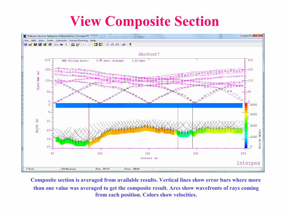
View Composite Section

Composite section is averaged from available results. Vertical lines show error bars where more than one value was averaged to get the composite result. Arcs show wavefronts of rays coming

from each position. Colors show velocities.

Add Labels for Velocity

Right-click on a point to add a label or label the velocity. Velocity labels show velocity at label center and this changes if the label is moved.

Discussion

The final section shows a relatively constant surface velocity, with a lower velocity near 100 m and again near 220 m.The highest refractor velocities lie between 90 and 160 m and again right of about 195 m. There is a low velocity zone from about 160-190 m.The refractor is deepest left of 90 m at about 22 m and shallower to the right of 90 m at about 15 m, including the low velocity section.What lies below the refractor is, of course, not determined by these data since no rays penetrate below that. Any areas shown in white are pretty much not well constrained.

Comparison

A comparison of the trimmed data set (below) with the full data set (above) shows they are quite similar. The left and right sides of the trimmed data set is more reasonable and closer to the true model. The low velocity zone near the right-center of the refractor is narrower in the second interpretationbut it does bleed to the right into the higher velocity section.The refractor surface seems a little rougher and the error bars are somewhat higher in the results from the trimmed data set.The trimmed data set has about 1/15th of the number of shots, so it would be considerably more cost effective from a logistics point of view.