Iterative computation of negative curvature...
24
Comput Optim Appl (2007) 38: 81–104 DOI 10.1007/s10589-007-9034-z Iterative computation of negative curvature directions in large scale optimization Giovanni Fasano · Massimo Roma Published online: 17 May 2007 © Springer Science+Business Media, LLC 2007 Abstract In this paper we deal with the iterative computation of negative curvature directions of an objective function, within large scale optimization frameworks. In particular, suitable directions of negative curvature of the objective function represent an essential tool, to guarantee convergence to second order critical points. However, an “adequate” negative curvature direction is often required to have a good resem- blance to an eigenvector corresponding to the smallest eigenvalue of the Hessian matrix. Thus, its computation may be a very difficult task on large scale problems. Several strategies proposed in literature compute such a direction relying on matrix factorizations, so that they may be inefficient or even impracticable in a large scale setting. On the other hand, the iterative methods proposed either need to store a large matrix, or they need to rerun the recurrence. On this guideline, in this paper we propose the use of an iterative method, based on a planar Conjugate Gradient scheme. Under mild assumptions, we provide theory for using the latter method to compute adequate negative curvature directions, within optimization frameworks. In our proposal any matrix storage is avoided, along with any additional rerun. Keywords Conjugate gradient method · Large scale optimization · Negative curvature directions · Convergence to second order critical points G. Fasano ( ) · M. Roma Dipartimento di Informatica e Sistemistica “A. Ruberti”, Università di Roma “La Sapienza”, via Buonarroti, 12, Roma, Italy e-mail: [email protected] M. Roma e-mail: [email protected] G. Fasano Istituto Nazionale per Studi ed Esperienze di Architettura Navale INSEAN, via di Vallerano, 139, Roma, Italy e-mail: [email protected]
Transcript of Iterative computation of negative curvature...

Comput Optim Appl (2007) 38: 81–104DOI 10.1007/s10589-007-9034-z
Iterative computation of negative curvature directionsin large scale optimization
Giovanni Fasano · Massimo Roma
Published online: 17 May 2007© Springer Science+Business Media, LLC 2007
Abstract In this paper we deal with the iterative computation of negative curvaturedirections of an objective function, within large scale optimization frameworks. Inparticular, suitable directions of negative curvature of the objective function representan essential tool, to guarantee convergence to second order critical points. However,an “adequate” negative curvature direction is often required to have a good resem-blance to an eigenvector corresponding to the smallest eigenvalue of the Hessianmatrix. Thus, its computation may be a very difficult task on large scale problems.Several strategies proposed in literature compute such a direction relying on matrixfactorizations, so that they may be inefficient or even impracticable in a large scalesetting. On the other hand, the iterative methods proposed either need to store a largematrix, or they need to rerun the recurrence.
On this guideline, in this paper we propose the use of an iterative method, basedon a planar Conjugate Gradient scheme. Under mild assumptions, we provide theoryfor using the latter method to compute adequate negative curvature directions, withinoptimization frameworks. In our proposal any matrix storage is avoided, along withany additional rerun.
Keywords Conjugate gradient method · Large scale optimization · Negativecurvature directions · Convergence to second order critical points
G. Fasano (�) · M. RomaDipartimento di Informatica e Sistemistica “A. Ruberti”, Università di Roma “La Sapienza”,via Buonarroti, 12, Roma, Italye-mail: [email protected]
M. Romae-mail: [email protected]
G. FasanoIstituto Nazionale per Studi ed Esperienze di Architettura Navale INSEAN,via di Vallerano, 139, Roma, Italye-mail: [email protected]

82 G. Fasano, M. Roma
1 Introduction
In this paper we tackle a general problem which arises in the definition of manyminimization methods: the computation of suitable negative curvature directions ofthe objective function, in large scale settings. Our interest is mainly motivated by thepossibility of using negative curvature directions, within linesearch based truncatedNewton methods, for large scale unconstrained optimization. However, the approachwe propose may be exploited in many different contexts of nonlinear programming.
We recall that, given a twice continuously differentiable real valued function f
and the point x ∈ Rn, the vector d ∈ R
n is a direction of negative curvature at x ifdT ∇2f (x)d < 0. The use of negative curvature directions in designing minimizationmethods has a twofold importance: from the theoretical point of view, convergencetowards second order critical points, i.e. stationary points where the Hessian matrixis positive semidefinite, may be guaranteed. From the computational point of view,observe that negative curvature directions exploit the local nonconvexities of the ob-jective function. Then, a descent negative curvature direction is such that the objec-tive function and its directional derivative are (locally) decreasing along it. Therefore,a step along a negative curvature direction, can hasten the search for a region wherethe objective function is convex.
The use of negative curvature directions in unconstrained optimization goes backup to [22] and the two landmark papers [21, 23], where linesearch based modifiedNewton methods were proposed. Here, a curvilinear path obtained by combininga Newton-type direction and a negative curvature direction was considered. Moreovera “second order” Armjio-type rule was used, to ensure the convergence to a secondorder critical point. The second order convergence can be ensured by exploiting thelocal curvatures of the objective function, contained in the second order derivatives.In particular, the negative curvature direction is required to resemble the eigenvectorcorresponding to the smallest eigenvalue λmin(∇2f (x)) of the Hessian matrix. For-mally, if xj denotes the current iterate of the algorithm in hand, the negative curvaturedirection dj must be nonascent and such that
(dj )T ∇2f (xj )dj → 0 implies min
[0, λmin(∇2f (xj )
)] → 0. (1.1)
Note that convergence to second order critical points is guaranteed also for the trustregion methods in unconstrained optimization (see, e.g. [3, 24, 28]): the latter resultstrongly motivates the interest for such methods.
The use of appropriate directions of negative curvature plays a key role also inconstrained optimization, when defining algorithms with convergence to points sat-isfying the second order KKT necessary optimality conditions (see, e.g. [6] and thereferences reported therein).
The computation of a nonascent direction of negative curvature dj , which sat-isfies (1.1), is a very difficult task, and the difficulty increases with the dimension.Indeed, in principle the computation of dj is equivalent to compute an eigenvectorcorresponding to the smallest eigenvalue of the Hessian matrix. In [23] the Bunchand Parlett factorization was proposed for determining a negative curvature direc-tion which satisfies (1.1). It was proved that the Bunch and Parlett decomposition,for a symmetric indefinite matrix, can be used for computing both a Newton-type

Iterative computation of negative curvature directions 83
direction and an adequate negative curvature direction. In [12] this approach was em-bedded in a nonmonotone framework, showing how its potentiality may be furtherexploited. In both cases, the computation of the negative curvature direction relies onmatrix factorizations, which are impracticable when dealing with large scale prob-lems. On the basis of this observation, in [19] a new strategy based on an iterativealgorithm was proposed, within truncated Newton schemes. The computation wasbased on the well known ability of the Lanczos algorithm, to efficiently determineextreme eigenpairs of an indefinite matrix. In particular, the SYMMLQ algorithm[26] was successfully used. However, here at step h ≤ n the negative curvature di-rection dj in (1.1) is computed as dj = Vhwh, where the h columns of Vh are theLanczos vectors and wh ∈ R
h. Therefore, the storage of matrix Vh is required, andin order to handle the large scale case, only a limited number of Lanczos vectorsare stored. Of course, this implies that dj is only approximately evaluated, and thesecond order convergence is no longer guaranteed.
In [15] a new approach for managing negative curvature directions, in large scaleunconstrained optimization, was introduced. In particular, a truncated Newton ap-proach was considered, where the alternate use of a Newton-type direction anda negative curvature direction was proposed. Then, an appropriate linesearch wasperformed on the chosen direction. To ensure condition (1.1) the strict connectionbetween the Conjugate Gradient (CG) and the Lanczos methods is exploited. Con-vergence to second order points is proved under mild assumptions, in such a way thatthe storage of any matrix is avoided. However, the price to pay is the necessity ofrerunning the recurrence, in order to regenerate the Lanczos vectors whenever theyare needed, similarly to the truncated Lanczos approach in [14].
A similar approach for iteratively computing a direction of negative curvature wasproposed in [2], where the authors discuss the possibility of using Lanczos, Cheby-shev and two-step Lanczos algorithms. As alternative to the storage of all the Lanc-zos vectors, they propose to store the two most recent vectors and to rerun the wholeLanczos process whenever necessary.
These considerations indicate the need of iterative methods, which computenonascent negative curvature directions satisfying (1.1), without storing any matrix.In this paper we focus on a variant of one of the most popular Krylov-based method,the CG method. As well known, it plays a central role in many implementations oftruncated Newton methods, due to its efficiency in determining a Newton-type direc-tion. Unfortunately the CG algorithm could untimely stop in the nonconvex case. Toovercome this drawback, the use of planar conjugate gradient algorithms has beenproposed [1, 5, 9, 10, 17, 18, 22]. Planar schemes are an extension of the linear CGmethod to the indefinite case. They iteratively perform the search of critical points ei-ther on mutually conjugate directions or planes, so that they are effective both in thedefinite and in the indefinite case. Such methods can be naturally embedded withinlarge scale unconstrained optimization, however they represent an important tool alsowithin other nonlinear optimization frameworks.
In this paper we propose the use of the planar CG method FLR, described in [9], inorder to iteratively compute, at each iteration of a truncated Newton method, a nega-tive curvature direction which satisfies condition (1.1), without requiring to store anymatrix and avoiding any rerun.
84 G. Fasano, M. Roma
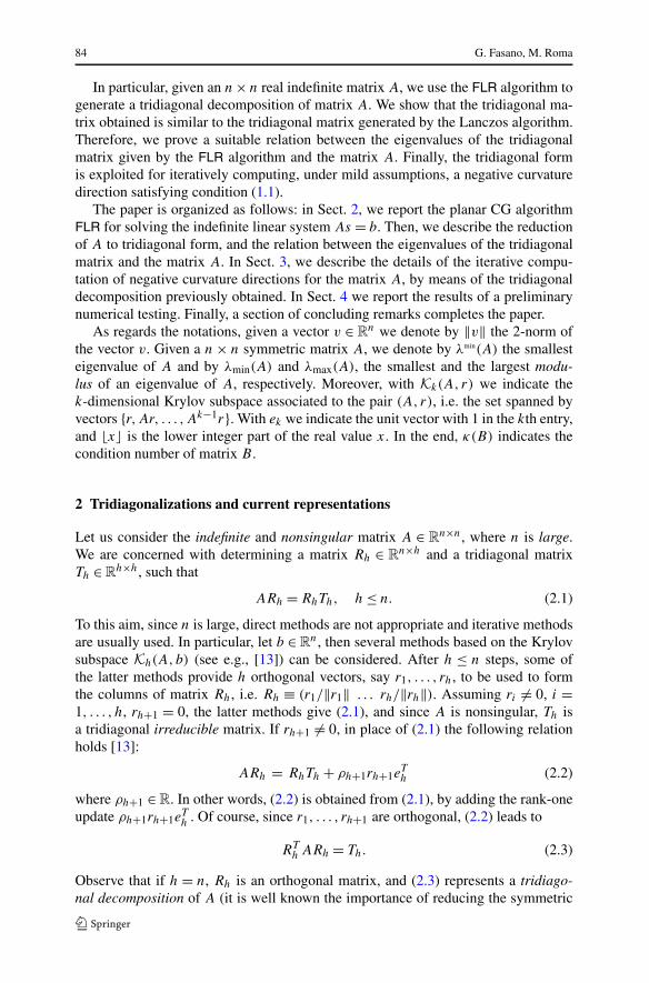
In particular, given an n × n real indefinite matrix A, we use the FLR algorithm togenerate a tridiagonal decomposition of matrix A. We show that the tridiagonal ma-trix obtained is similar to the tridiagonal matrix generated by the Lanczos algorithm.Therefore, we prove a suitable relation between the eigenvalues of the tridiagonalmatrix given by the FLR algorithm and the matrix A. Finally, the tridiagonal formis exploited for iteratively computing, under mild assumptions, a negative curvaturedirection satisfying condition (1.1).
The paper is organized as follows: in Sect. 2, we report the planar CG algorithmFLR for solving the indefinite linear system As = b. Then, we describe the reductionof A to tridiagonal form, and the relation between the eigenvalues of the tridiagonalmatrix and the matrix A. In Sect. 3, we describe the details of the iterative compu-tation of negative curvature directions for the matrix A, by means of the tridiagonaldecomposition previously obtained. In Sect. 4 we report the results of a preliminarynumerical testing. Finally, a section of concluding remarks completes the paper.
As regards the notations, given a vector v ∈ Rn we denote by ‖v‖ the 2-norm of
the vector v. Given a n × n symmetric matrix A, we denote by λmin(A) the smallesteigenvalue of A and by λmin(A) and λmax(A), the smallest and the largest modu-lus of an eigenvalue of A, respectively. Moreover, with Kk(A, r) we indicate thek-dimensional Krylov subspace associated to the pair (A, r), i.e. the set spanned byvectors {r,Ar, . . . ,Ak−1r}. With ek we indicate the unit vector with 1 in the kth entry,and �x� is the lower integer part of the real value x. In the end, κ(B) indicates thecondition number of matrix B .
2 Tridiagonalizations and current representations
Let us consider the indefinite and nonsingular matrix A ∈ Rn×n, where n is large.
We are concerned with determining a matrix Rh ∈ Rn×h and a tridiagonal matrix
Th ∈ Rh×h, such that
ARh = RhTh, h ≤ n. (2.1)
To this aim, since n is large, direct methods are not appropriate and iterative methodsare usually used. In particular, let b ∈ R
n, then several methods based on the Krylovsubspace Kh(A,b) (see e.g., [13]) can be considered. After h ≤ n steps, some ofthe latter methods provide h orthogonal vectors, say r1, . . . , rh, to be used to formthe columns of matrix Rh, i.e. Rh ≡ (r1/‖r1‖ . . . rh/‖rh‖). Assuming ri = 0, i =1, . . . , h, rh+1 = 0, the latter methods give (2.1), and since A is nonsingular, Th isa tridiagonal irreducible matrix. If rh+1 = 0, in place of (2.1) the following relationholds [13]:
ARh = RhTh + ρh+1rh+1eTh (2.2)
where ρh+1 ∈ R. In other words, (2.2) is obtained from (2.1), by adding the rank-oneupdate ρh+1rh+1e
Th . Of course, since r1, . . . , rh+1 are orthogonal, (2.2) leads to
RTh ARh = Th. (2.3)
Observe that if h = n, Rh is an orthogonal matrix, and (2.3) represents a tridiago-nal decomposition of A (it is well known the importance of reducing the symmetric

Iterative computation of negative curvature directions 85
matrix A to the tridiagonal form Th). Relation (2.2) will be referred in the sequel ascurrent representation of the symmetric matrix A.
The CG and the Lanczos methods are among the most commonly used Krylovsubspace methods to give (2.3). In the case of the CG method, the vector ri , i ≤ n,is the residual generated at iteration i − 1. The Lanczos method directly calculatesorthonormal vectors (the Lanczos vectors) which can be used as columns of the ma-trix Rh. The two methods, along with their equivalence, have been deeply studied(see, e.g., [3, Sect. 5.2], [4, 13, 29]). We only recall that if A is positive definite, thenTh is positive definite too, so that the tridiagonal matrix Th can be stably factorizedin the form
Th = LhDhLTh (2.4)
where Lh is a unit lower bidiagonal matrix and Dh is diagonal. Furthermore, theentries of the matrix Lh and the diagonal elements of the matrix Dh can be easilyrecovered from the quantities generated by the CG or the Lanczos algorithms (see,e.g., [29]).
If A is indefinite, the factorization (2.4) may fail—in the sense that it may not existor may be very unstable—and a stable indefinite factorization must be alternativelyconsidered. Such a decomposition is based on factorizing the tridiagonal matrix Th
in the form
Th = LhBhLTh (2.5)
where Lh is a unit lower bidiagonal matrix, while Bh is a block diagonal—and nolonger a diagonal matrix. Each diagonal block of Bh is 1 × 1 or 2 × 2, hence theprocedure to obtain the decomposition (2.5) is definitely more cumbersome.
In this paper, in order to obtain relations (2.2) and (2.3), we propose the use of theplanar-CG algorithm FLR [9], which is a modification of the planar CG algorithmproposed in [17]. It is an extension of the standard CG algorithm to the indefinitecase; moreover it enables to overcome the well known drawbacks due to possiblepivot breakdowns.
2.1 A planar-CG algorithm
In this section we briefly describe the planar CG algorithm FLR proposed in [9] andreported in Table 1, which will be used to obtain relations (2.1–2.3). This scheme isa modification of the algorithm proposed by Hestenes in [17]. An extensive descrip-tion of the FLR algorithm can be found in [9, 10]; here we report some new relatedresults, which arise from the application of the FLR algorithm within optimizationframeworks. (We highlight that the role of the logical variable CR, introduced in Ta-ble 1, will be clarified in Sect. 3.3.)
Firstly, suppose the matrix A is positive definite; as long as at Step k we haveεk ≤ λmin(A), the planar CG Step kB is never performed, therefore the algorithm re-duces to the standard CG. On indefinite linear systems the FLR algorithm overcomesthe well known drawback of the standard CG, which may untimely stop. The lat-ter result is accomplished by detecting the critical point of the associated quadraticfunction f (x) = 1/2xT Ax − bT x on mutually conjugate directions or planes. This isa common feature of all the planar CG methods (see [9] and the references reported

86 G. Fasano, M. Roma
Table 1 Algorithm FLR for solving the linear system As = b
Algorithm FLR
Step 1: k = 1, s1 = 0, r1 = b, CR = false. If r1 = 0 then CR = true and STOP,
else compute p1 = r1.
Step k: Compute σk = pTk Apk .
If | σk |≥ εk‖pk‖2 then go to Step kA else go to Step kB
– Step kA (standard CG step):
Set sk+1 = sk + akpk , rk+1 = rk − akApk , where ak = rTk pk
σk.
If rk+1 = 0 then CR = true and STOP
else compute pk+1 = rk+1 + βkpk with βk = −pTk Ark+1σk
= ‖rk+1‖2
‖rk‖2 .Set k = k + 1 and go to Step k.
– Step kB (planar CG step):If k = 1 then compute the vector qk = Apk ,else compute the vector
qk =
⎧⎪⎪⎨
⎪⎪⎩
Apk + bk−1pk−1, if the previous step is Step (k − 1)A
Apk + bk−2�k−2
(σk−2qk−2 − δk−2pk−2),
if the previous step is Step (k − 2)B
where bk−1 = −(Apk−1)T Apk/σk−1 and bk−2 = −(Aqk−2)
T Apk .
Compute ck = rTk pk , δk = pT
k Aqk , ek = qTk Aqk , �k = σkek − δ2
k
and ck = (ckek − δkqTk rk)/�k , σk = (σkq
Tk rk − δkck)/�k .
Set sk+2 = sk + ckpk + σkqk , rk+2 = rk − ckApk − σkAqk .
If rk+2 = 0 then CR = true and STOP
else compute pk+2 = rk+2 + βk
�k(σkqk − δkpk) with βk = −qT
k Ark+2.
Set k = k + 2 and go to Step k.
therein). In particular, assuming that the matrix A is indefinite and nonsingular, byapplying the standard CG, pivot breakdown occurs at Step k if pT
k Apk = 0, so thatthe iterates are terminated prematurely. On the contrary, planar CG methods generateanother direction at Step kB (denoted by qk). Then, instead of detecting the criticalpoint along the line xk + αpk , α ∈ R (which is carried on at Step kA), they performa search on the 2-dimensional linear manifold xk + span{pk, qk}. More specifically,as concerns the FLR algorithm, it can be easily proved (see Lemma 2.2 in [9]) that, ifthe matrix A is nonsingular and at Step k we have rk = 0, the FLR algorithm can al-ways perform either Step kA or Step kB . For further properties of the sequences {pk}and {qk} we refer to Theorem 2.1 in [9]. As regards the parameter εk at the Step k

Iterative computation of negative curvature directions 87
(see also [9]), let ε ∈ R be positive, then the choice
ε < εk, at Step kA,
ε < εk ≤ εk = min
{2
3λmin(A)
‖rk‖‖pk‖ , λ2
max(A)‖pk‖‖qk‖ ,
λ4min(A)
2λmax(A)
‖pk‖2
‖qk‖2
}, (2.6)
at Step kB,
guarantees the denominators at Step kA and Step kB to be sufficiently bounded awayfrom zero. We highlight that the choice (2.6) is slightly stronger than the choice ofthe parameter εk at Step k of the FLR algorithm in [9]. As regards the apparentlycumbersome computation of the quantity ‖qk‖ in (2.6), no additional cost is needed(see also [9]). In the sequel we assume that at Step k the parameter εk satisfies con-dition (2.6).
2.2 Tridiagonalizations and current representations via the FLR algorithm
In this section we describe how to obtain a tridiagonal decomposition and a cur-rent representation of the matrix A, by means of the FLR algorithm. As regards thesequence of the directions generated by this algorithm, we adopt the following no-tation: if at Step k the condition |pT
k Apk| ≥ εk‖pk‖2 is satisfied, then set wk = pk
(standard CG step) otherwise set wk = pk and wk+1 = qk (planar CG step). With thelatter convention, {wi} represents the sequence of directions generated by the FLRalgorithm.
Observe that the sequence of the residuals {ri} is necessary to form the matrix Rh
in (2.3); however, note that in the planar CG Step kB , the vector rk+1 is not generated.The latter shortcoming may be overcome by introducing a “dummy” residual rk+1,which completes the sequence of orthogonal vectors r1, . . . , rk, rk+1, rk+2, . . . , rh[1, 7]. It is easy to see that the only possible choice (apart from a scale factor) forthe dummy residual rk+1, such that rk+1 ∈ Kk(A, r1) and rk+1 /∈ Kk−1(A, r1), is thefollowing [7]:
rk+1 = αkrk + (1 + αk) sgn(σk)Apk, αk = − |σk|‖rk‖2 + |σk| (2.7)
where the coefficient αk is computed by imposing the orthogonality conditionrTk+1pk = rT
k+1rk = 0. We highlight that since ‖rk‖ and ‖Apk‖ are bounded, ‖rk+1‖is bounded too. Moreover, from (2.7) and [9, Theorem 2.1], it can be readily seen thatthe dummy residual rk+1 satisfies also the required orthogonality properties
rTk+1ri = 0, i ≤ k, and rT
i rk+1 = 0, i > k + 1.
Now, we show that the FLR algorithm yields both the tridiagonalization (2.3) andthe current representation (2.2), when matrix A is indefinite. To this aim suppose thatthe FLR algorithm performs up to step h and, for the sake of simplicity, the onlyone planar CG step is Step kB < h. Then, considering (2.7) and the instructions atStep kB , along with the position
Rh =(
r1
‖r1‖ · · · rh
‖rh‖)
∈ Rn×h, Ph =
(w1
‖r1‖ · · · wh
‖rh‖)
∈ Rn×h,

88 G. Fasano, M. Roma
the following result can be obtained:
Theorem 2.1 Consider the FLR algorithm and let ‖ri‖ = 0, i ≤ h. Suppose the onlyone planar CG step is Step kB < h. Then the following relations hold:
PhLTh = Rh, (2.8)
APh =(
Rh
...rh+1
‖rh+1‖)(
Lh
lh+1,heTh
)Dh, h < n, (2.9)
ARh =(
Rh
...rh+1
‖rh+1‖)(
Th
th+1,heTh
), h < n, (2.10)
where
Lh =
⎛
⎜⎜⎜⎜⎜⎜⎜⎜⎜⎜⎜⎜⎜⎜⎜⎜⎜⎜⎜⎝
1
−√β1 ·
· 1
−√βk−1 1 0
α1 α2
α3 α4 1
0 −√βk+2 ·
· 1
−√βh−1 1
⎞
⎟⎟⎟⎟⎟⎟⎟⎟⎟⎟⎟⎟⎟⎟⎟⎟⎟⎟⎟⎠
(2.11)
with (βk = ‖rk+1‖2/‖rk‖2, βk+1 = ‖rk+2‖2/‖rk+1‖2)
α1 = αk√βk
, α2 = (1 + αk) sgn(σk),
α3 = βkδk
�k
√βk+1βk
, α4 = − βk σk
�k
√βk+1
,
(2.12)
Dh =
⎛
⎜⎜⎜⎜⎜⎜⎜⎜⎜⎜⎜⎝
1a1 ·
1ak−1
01ξk
1ξk+1
0 1ak+2 ·
1ah
⎞
⎟⎟⎟⎟⎟⎟⎟⎟⎟⎟⎟⎠
, (2.13)
Iterative computation of negative curvature directions 89
Lh =
⎛
⎜⎜⎜⎜⎜⎜⎜⎜⎜⎜⎜⎜⎜⎜⎜⎜⎜⎜⎜⎝
1
−√β1 ·
· 1 0
−√βk−1 α1 α3
α2 α4
α5 1
0 −√βk+2 ·
· 1
−√βh−1 1
⎞
⎟⎟⎟⎟⎟⎟⎟⎟⎟⎟⎟⎟⎟⎟⎟⎟⎟⎟⎟⎠
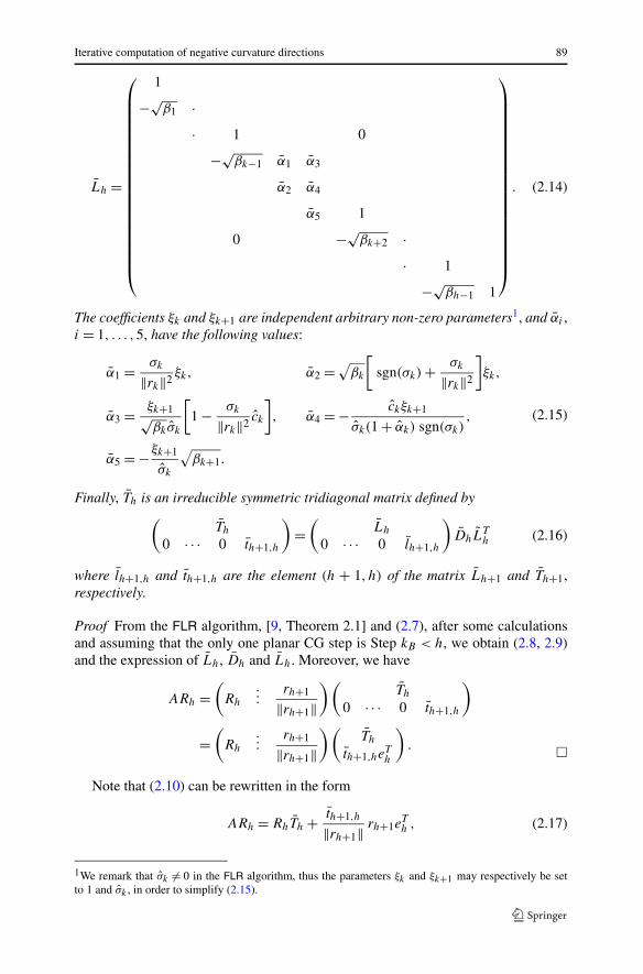
. (2.14)
The coefficients ξk and ξk+1 are independent arbitrary non-zero parameters1, and αi ,i = 1, . . . ,5, have the following values:
α1 = σk
‖rk‖2ξk, α2 = √
βk
[sgn(σk) + σk
‖rk‖2
]ξk,
α3 = ξk+1√βkσk
[1 − σk
‖rk‖2ck
], α4 = − ckξk+1
σk(1 + αk) sgn(σk),
α5 = −ξk+1
σk
√βk+1.
(2.15)
Finally, Th is an irreducible symmetric tridiagonal matrix defined by(
Th
0 · · · 0 th+1,h
)=
(Lh
0 · · · 0 lh+1,h
)DhL
Th (2.16)
where lh+1,h and th+1,h are the element (h + 1, h) of the matrix Lh+1 and Th+1,respectively.
Proof From the FLR algorithm, [9, Theorem 2.1] and (2.7), after some calculationsand assuming that the only one planar CG step is Step kB < h, we obtain (2.8, 2.9)and the expression of Lh, Dh and Lh. Moreover, we have
ARh =(
Rh
...rh+1
‖rh+1‖)(
Th
0 · · · 0 th+1,h
)
=(
Rh
...rh+1
‖rh+1‖)(
Th
th+1,heTh
). �
Note that (2.10) can be rewritten in the form
ARh = RhTh + th+1,h
‖rh+1‖ rh+1eTh , (2.17)
1We remark that σk = 0 in the FLR algorithm, thus the parameters ξk and ξk+1 may respectively be setto 1 and σk , in order to simplify (2.15).

90 G. Fasano, M. Roma
which is a current representation of the indefinite nonsingular matrix A. The follow-ing result provides further theoretical properties of the matrix Lh, which will be usedlater on.
Proposition 2.2 Consider the FLR algorithm and let ‖ri‖ = 0, i ≤ h, where h < n.Suppose that λmin(A) ≥ γ > 0, γ ∈ R, and that ν ≥ 0 planar CG steps are performed.Let the parameter εk satisfy condition (2.6), with k ≤ h. Then, the matrix Lh in (2.11)is nonsingular and ‖Lh‖ is bounded. Moreover, the following relations hold
(1
1+4λ2min(A)/(9ε)
)ν
≤ |det(Lh)| ≤ 1, (2.18)
‖Lh‖ ≤ �max
[(2h − 1) + h
2
]1/2
where (2.19)
�max = max k∈{j1,...,jν }i=1,...,h−1, i =k,k+1
{√βi,2,2
√βk+1βk,2 εk
λ2min(A)
βk
√βk+1
}, (2.20)
�max is bounded, j1, . . . , jν are the indices of the planar CG steps and jp ≤ h − 1,p = 1, . . . , ν.
For the sake of brevity, we do not report here the proof of this result for which werefer to [11].
As we already discussed, several methods may be used to reduce the matrix A
to a tridiagonal form. Furthermore, it can be worthwhile to point out to what ex-tent the tridiagonal matrix generated depends on the method. On this guideline theTheorem 7-2-2 in [27] allows us to immediately derive the following proposition,concerning the FLR algorithm.
Proposition 2.3 Let A ∈ Rn×n be symmetric and indefinite. Suppose to perform the
FLR algorithm and generate the orthogonal matrix Rn = (r1/‖r1‖ . . . rn/‖rn‖),along with the irreducible tridiagonal matrix Tn, such that ARn = RnTn. Then, Tn
and Rn are uniquely determined by A and r1/‖r1‖ or, alternatively, by A and rn/‖rn‖.
2.3 Relationship between the eigenvalues of matrices Th and A
Suppose now to apply the Lanczos algorithm to the linear system As = b, withb ∈ R
n. Then, after n steps the Lanczos algorithm generates the orthogonal matrixVn = (v1, . . . , vn) and the tridiagonal matrix Tn, such that AVn = VnTn. Similarly toProposition 2.3, by Theorem 7-2-2 in [27] we have that Tn and Vn are uniquely deter-mined by A and v1, or alternatively by A and vn. However, this does not imply that thetridiagonal matrices Tn (from the Lanczos process) and Tn (from the FLR algorithm)coincide. It rather suggests that the vectors ri/‖ri‖ and vi , i ≤ n, are parallel. Thus,the sequences {vi} and {ri/‖ri‖} are orthonormal bases of the same Krylov subspace,and vi = θi ri/‖ri‖, with θi ∈ {−1,+1}. The sequence {θi} is uniquely defined. Inparticular, in case no planar CG steps are performed (the FLR algorithm reduces tothe standard CG), the detailed calculus of θi can be found, e.g., in [3, Sect. 5.2.2].

Iterative computation of negative curvature directions 91
When planar CG steps are performed in the FLR algorithm, the expression of θi isreported in [8]. This implies that the following relation holds
Th = V Th AVh = �T
h RTh ARh�h = �hTh�h, h ≤ n, (2.21)
where �h = diag{θi, i = 1, . . . , h} is nonsingular. Due to the similarity (2.21), someimportant relations between the eigenvalues of matrices Th and A hold from the rela-tion between Th and A. Therefore, properties on the eigenvalues of Th can be directlyinherited from the properties of the eigenvalues of Th. We now briefly describe therelation between the smallest eigenvalue of the tridiagonal matrix Th in (2.16), andthe eigenvalues of matrix A. This will provide a tool for estimating the eigenvectorof A associated to the smallest eigenvalue of matrix A. Then, the latter vector will beused to compute a suitable negative curvature direction in optimization frameworks.
Theorem 2.4 Let λ1(A) ≤ · · · ≤ λn(A) be the ordered eigenvalues of the matrix A.Moreover, let μ1(Th) ≤ · · · ≤ μh(Th) be the ordered eigenvalues of the matrix Th.Then the following statements hold.
(i) The inequality λ1(A) ≤ μ1(Th) ≤ λ1(A) + C
φ2h−1(1+2ρ)
, holds where C is a pos-
itive scalar, φh−1 is the h − 1 degree Chebyshev polynomial and ρ = (λ2(A) −λ1(A))/(λn(A) − λ2(A)).
(ii) Let rh = 0 and rh+1 = 0, then the eigenvalues μ1(Th) ≤ · · · ≤ μh(Th) of thematrix Th are also eigenvalues of matrix A, and μ1(Th) < μ1(Th−1) < · · · <
μh−1(Th−1) < μh(Th). Moreover if u(h)i is the eigenvector of Th correspond-
ing to the eigenvalue μi(Th), then the vector Rhu(h)i is an eigenvector of the
matrix A.(iii) There exists an eigenvalue λ(A) ∈ R of matrix A such that
∣∣λ(A) − μi(Th)∣∣ ≤ |th+1,h|.
Proof It is well known that properties (i) and (ii) hold if we consider the tridiago-nal matrix Th generated by the Lanczos algorithm (see e.g. [13]). Hence, from thesimilarity (2.21) they hold for the tridiagonal matrix Th.
As regards (iii), suppose (μi(Th), u(h)i ) is an eigenpair of matrix Th, i ≤ h with
‖u(h)i ‖ = 1. Then, by Theorem 4-5-1 in [27] and (2.17), an eigenvalue λ(A) of A
exists such that:
|λ(A) − μi(Th)| ≤ ‖ARhu(h)i − μi(Th)Rhu
(h)i ‖
‖Rhu(h)i ‖
= ∥∥(ARh − RhTh)u(h)i
∥∥
=∥∥∥∥th+1,h
rh+1
‖rh+1‖eTh u
(h)i
∥∥∥∥ ≤ |th+1,h|. (2.22)
�
Observe that from property (i), the smallest eigenvalue of the tridiagonal matrixTh approaches very quickly the smallest eigenvalue of the matrix A (see also [30,p. 279]).

92 G. Fasano, M. Roma
Property (ii) yields μ1(Th) < μ1(Th−1) therefore, at each iteration the FLR algo-rithm improves the estimate of the smallest eigenvalue of the matrix A, by means of(2.17) and (2.22).
Finally, property (iii) shows that if |th+1,h| is sufficiently small, the quantityμi(Th) is a good approximation of the eigenvalue λ(A) of matrix A (we recall thatwhen th+1,h = 0 the FLR algorithm stops).
3 Iterative computation of negative curvature directions
In this section we use the theory developed in the previous sections within truncatedNewton frameworks. We recall that the latter iterative schemes have proved to beeffective tools for large scale optimization problems (see, e.g., [25]). In particular,in unconstrained optimization, convergence towards second order stationary pointswhere the Hessian is positive semidefinite, can be ensured by computing, at eachiteration j , a pair of directions (sj , dj ). The direction sj is a Newton-type directionobtained by approximately solving the Newton’s system ∇2f (xj ) s = −∇f (xj ),whose purpose is to guarantee the convergence to stationary points. The direction dj
is a suitable negative curvature direction used to force convergence to second orderstationary points [19, 23]. This requires that the sequence {dj } satisfies the followingassumption.
Condition A The directions {dj } are bounded and such that
(dj )T ∇2f (xj )dj < 0, (3.1)
(dj )T ∇2f (xj )dj → 0 implies min
[0, λmin(∇2f (xj ))
] → 0, (3.2)
where λmin(∇2f (xj )) is the smallest eigenvalue of the Hessian matrix ∇2f (xj ).
Here we describe how to compute such directions {dj } by using the theory devel-oped in the previous sections. More specifically, we describe how to exploit relation(2.17), obtained in Sect. 2 via the FLR algorithm, for iteratively computing directiondj in order to satisfy Condition A.
To this aim, we focus on a generic iteration j of a truncated Newton method andwe consider the matrix A as the system matrix at the j th iteration of the method(in the unconstrained optimization case As = b is the Newton’s system at the j thiteration with A = ∇2f (xj )). Now, suppose to apply the FLR algorithm and that itterminates after n steps, i.e. the condition rn+1 = 0 is fulfilled and formulae (2.8) and(2.9) hold with h = n. Observe that in a large scale setting, when far from the solution,the FLR algorithm should possibly avoid to completely investigate an n-dimensionalKrylov subspace. Thus, in general it may be impossible to guarantee condition (3.2)because (see [15, Sect. 4]) “. . . the Krylov subspace investigated may not contain anyeigenvector corresponding to the leftmost eigenvalue. However [in a truncated New-ton scheme, when close to a stationary point] this happens with probability zero inexact arithmetic, and we don’t expect it to happen in presence of rounding.” There-fore, we carry on a theoretical analysis under the assumption that the FLR algorithmperforms exactly n steps, while in practice, we will compute the direction dj after

Iterative computation of negative curvature directions 93
a smaller number of steps. The numerical experience in Sect. 4 gives evidence thatthe latter approach is effective and efficient.
On this guideline, condition rn+1 = 0 in (2.17) yields ARn = RnTn. So that from(2.16), we have the following factorization for the symmetric tridiagonal matrix Tn
Tn = LnDnLTn (3.3)
where Ln and Ln are given in (2.11) and (2.14) (with h = n). Note that in generalLn = Ln, unless no planar CG steps were performed by the FLR algorithm. Sinceboth Ln and Ln are nonsingular, the nonsingular matrix �n ∈ R
n×n exists such that
Ln = Ln�n. (3.4)
Now, w.l.o.g. assume that only one planar CG step was performed and it was Step kB ;then, the explicit expression of �n is given by
�n =
⎛
⎜⎜⎜⎜⎜⎜⎜⎜⎜⎜⎜⎜⎝
1. . . 0
1πk,k πk,k+1
πk+1,k πk+1,k+1
1
0. . .
1
⎞
⎟⎟⎟⎟⎟⎟⎟⎟⎟⎟⎟⎟⎠
, (3.5)
with
πk,k = α1, πk,k+1 = α3,
πk+1,k = α2 − α1α1
α2, πk+1,k+1 = α4 − α3α1
α2
(3.6)
where αi and αi , i ≤ 4, are given in (2.12) and (2.15). Hence, by (3.3) and (3.4)
Tn = Ln(�nDn)LTn , (3.7)
and it is easy to verify that the block diagonal matrix �nDn is symmetric.The importance of the factorization (3.7) in computing the negative curvature di-
rection dj , for matrix A, relies on the following facts:
• the computation of the eigenpairs of �nDn is trivial. Furthermore it is possible toestablish a simple relation between the eigenvalues of Tn and the eigenvalues of�nDn;
• since ri = 0, i = 1, . . . , n and rn+1 = 0, the matrix Tn is irreducible and theeigenvalues μ1(Tn) < · · · < μn(Tn) of Tn are also eigenvalues of matrix A (Theo-rem 2.4).
Now let us state the following technical proposition.

94 G. Fasano, M. Roma
Proposition 3.1 Consider the solution y of the linear system LTn y = z1, where Ln
is given in (2.11) and z1 is the normalized eigenvector corresponding to the smallesteigenvalue of �nDn (see (2.13) and (3.5)). Let ν ≥ 0 be the number of the planar CGsteps performed by the FLR algorithm. Let �max be an upper bound for the modulusof the entries of matrix Ln. Assume that εk in the FLR algorithm satisfies (2.6). Thenthe vector y is bounded and satisfies
‖y‖ ≤ n2ν(�max)n−1
√
(n − ν) + ν
(1 + 4
9
λ2min(A)
ε
)2
where
�max =(
1 + 4
9
λ2min(A)
ε
)�max.
For the sake of brevity, we do not report here the proof of this result for which werefer to [11].
The next theorem, which follows from [23, Lemma 4.3], shows how to determinea direction of negative curvature by means of the decomposition (3.7).
Theorem 3.2 Let us consider the decomposition (3.7), where Tn has at least one neg-ative eigenvalue. Let z1 be the normalized eigenvector corresponding to the smallesteigenvalue of �nDn, and y ∈ R
n the solution of the linear system
LTn y = z1. (3.8)
Then the vector
dj = Rny (3.9)
is a bounded negative curvature direction satisfying (3.1) and (3.2).
Proof From relation (2.3) with h = n and considering that μmin(Tn) is the smallesteigenvalue of Tn, Lemma 4.3 in [23] yields
0 > μmin(Tn) ≥ (yT Tny
)‖Ln‖2 ≥ [κ(Ln)
]2 (yT Tny)
‖y‖2
= [κ(Ln)
]2 [(Rny)T A(Rny)]‖Rny‖2
. (3.10)
Finally, from Theorem 2.4 the smallest eigenvalue λmin(A) of A satisfies λmin(A) =μmin(Tn), then
0 > λmin(A) ≥ [κ(Ln)
]2 [(Rny)T A(Rny)]‖Rny‖2
, (3.11)
i.e. dj is a negative curvature direction and (3.2) holds. Now we show that the direc-tion dj defined in (3.9) is bounded. On this purpose, considering that Rn is orthog-onal, dj is bounded as long as the solution y of the linear system (3.8) is bounded.The latter result is stated in Proposition 3.1. �

Iterative computation of negative curvature directions 95
Now observe that, according to (3.9), the computation of dj requires the storageof both the vector y and the full rank matrix Rn. Unfortunately this is unpractical forlarge scale problems. Here we show that both the computation of y and the storage ofRn may be avoided, so that the FLR algorithm iteratively provides the vector dj . Wedistinguish between the (simpler) case in which no planar CG steps are performed,from the case where planar CG steps are performed.
3.1 No planar CG steps are performed in the FLR algorithm
If no planar CG steps are performed, in Proposition 3.1 we have z1 = em, for a certainm ≤ n. Moreover, the decomposition (3.3) becomes Tn = LnDnL
Tn , where [29]
Ln =
⎛
⎜⎜⎜⎜⎜⎜⎜⎝
1 0−√
β1 1
· ·
· 10 −√
βn−1 1
⎞
⎟⎟⎟⎟⎟⎟⎟⎠
and Dn = diag{1/a1, . . . ,1/an}. Therefore, recalling relation βi = ‖ri+1‖2/‖ri‖2,i ≤ n − 1, the solution y = (y1 . . . yn)
T of the linear system (3.8) can be obtained bybacktracking from yn to y1. In particular, we have
yn = · · · = ym+1 = 0, ym = 1, and
ym−1 = ‖rm‖‖rm−1‖ , ym−2 = ‖rm‖
‖rm−2‖ , . . . , y1 = ‖rm‖‖r1‖ .
From (3.9), recalling that pi = ri + βi−1pi−1, i ≤ n, we simply obtain
dj = ‖rm‖m∑
i=1
ri
‖ri‖2= pm
‖rm‖ . (3.12)
The difficulty that m is not known “a priori,” can be easily overcome, since m is theindex of the least negative diagonal entry of matrix Dn, i.e. 1/am ≤ 1/ai , for anyai < 0, i ≤ n. Hence, from (3.12) the calculation of dj may be easily carried oniteratively and requires the storage of only one additional vector.
3.2 Some planar CG steps are performed in the FLR algorithm
In case some planar CG steps are performed by the FLR algorithm, the structure ofmatrix Ln in (3.8) is given in (2.11) with h = n. Now, we manipulate (3.7) so that
Ln = LnDn and Tn = LnBnLTn (3.13)
where Dn is a nonsingular diagonal matrix and Ln is a nonsingular unit lower triangu-lar matrix (see [11] for the exact definition of Dn and Ln). Then, Bn = Dn�nDnDn

96 G. Fasano, M. Roma
is a block diagonal matrix with 1 × 1 and 2 × 2 nonsingular blocks. From Proposi-tion 3.1 and its proof we observe that w.l.o.g., in place of solving the linear system(3.8) in Theorem 3.2, we can consider equivalently from (3.13) the system
LTn y = z1 (3.14)
where now z1 is the normalized eigenvector corresponding to the least negative eigen-value of Bn. The vector z1 may have two different expressions:
(1) if the smallest negative eigenvalue of Bn is a 1 × 1 diagonal block of matrix Bn
(corresponding to a standard CG step in the FLR algorithm), then z1 = em fora certain m ≤ n;
(2) otherwise, let λm,λm+1 be eigenvalues of Bn, corresponding to a 2 × 2 diagonalblock (planar CG step in the FLR algorithm), with λm ≤ λm+1. Then, if λm is thesmallest eigenvalue of Bn, it results z1 = (0, . . . ,0,ωm,ωm+1,0, . . . ,0)T whereωm, ωm+1 ∈ R and can be trivially calculated.
Therefore, as in the previous section we want to determine the solution y of (3.14)and the direction dj of (3.9) in either the cases above, assuming that some planar CGsteps were performed.
• We first consider the case (1) in which
z1 = em, (3.15)
i.e. the smallest eigenvalue of Bn corresponds to a standard CG step in the FLRalgorithm. By simply backtracking from yn to y1 we obtain (see (3.14))
yn = · · · = ym+1 = 0.
Then, we compute yi , i = 1, . . . ,m, by checking whether Step i, i = 1, . . . ,m,was a standard CG step or a planar CG step. In particular, suppose w.l.o.g. thatthe FLR algorithm performed the standard CG steps mA, (m − 1)A, . . . , (h + 2)A,
(h − 1)A, . . . ,1A, and the only one planar CG step hB . Then, it is possible to verifythat by backtracking from index i = m, we have from (3.14)
yi = ‖rm‖‖ri‖ , i = m, . . . , h + 2,
yh+1 = ‖rm‖‖rh+2‖�
(h)1 ,
yh = ‖rm‖‖rh+2‖�
(h)2 ,
yi = ‖rm‖‖rh+2‖�
(h)2
‖rh‖‖ri‖ , i = h − 1, . . . ,1,
(3.16)
where
�(h)1 = − α
(h)4
α(h)2
, �(h)2 = α
(h)1 α
(h)4
α(h)2
− α(h)3 . (3.17)
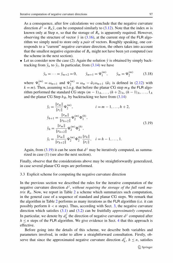
Iterative computation of negative curvature directions 97
As a consequence, after few calculations we conclude that the negative curvaturedirection dj = Rny, can be computed similarly to (3.12). Note that the index m isknown only at Step n, so that the storage of Rn is apparently required. However,observing the structure of vector y in (3.16), at the current step of the FLR algo-rithm we simply need to store only a pair of vectors. Roughly speaking, one cor-responds to a “current” negative curvature direction, the others takes into accountthat the smallest negative eigenvalue of Bn might not have been yet computed (seethe scheme in the next section).
• Let us consider now the case (2). Again the solution y is obtained by simply back-tracking from yn to y1. In particular, from (3.14) we have
yn = · · · = ym+2 = 0, ym+1 = �(m)1 , ym = �
(m)2 (3.18)
where �(m)1 = ωm+1 and �
(m)2 = ωm − α1ωm+1 (α1 is defined in (2.12) with
k = m). Then, assuming w.l.o.g. that before the planar CG step mB the FLR algo-rithm performed the standard CG steps (m − 1)A, . . . , (h + 2)A, (h − 1)A, . . . ,1A
and the planar CG Step hB , by backtracking we have from (3.14)
yi = ‖rm‖‖ri‖ �
(m)2 , i = m − 1, . . . , h + 2,
yh+1 = ‖rm‖‖rh+2‖�
(m)2 �
(h)1 ,
yh = ‖rm‖‖rh+2‖�
(m)2 �
(h)2 ,
yi = ‖rm‖‖rh+2‖�
(m)2 �
(h)2
‖rh‖‖ri‖ , i = h − 1, . . . ,1.
(3.19)
Again, from (3.19) it can be seen that dj may be iteratively computed, as summa-rized in case (1) (see also the next section).
Finally, observe that the considerations above may be straightforwardly generalized,in case several planar CG steps are performed.
3.3 Explicit scheme for computing the negative curvature direction
In the previous section we described the rules for the iterative computation of thenegative curvature direction dj , without requiring the storage of the full rank ma-trix Rn. Now, we report in Table 2 a scheme which summarizes such computation,in the general case of a sequence of standard and planar CG steps. We remark thatthe algorithm in Table 2 performs as many iterations as the FLR algorithm (i.e. it canpossibly perform h < n steps). Thus, according with Sect. 3, the negative curvaturedirection which satisfies (3.1) and (3.2) can be fruitfully approximately computed.In particular, we denote by d
jh the direction of negative curvature dj computed after
h ≤ n steps of the FLR algorithm. We give evidence in Sect. 4 that this approach iseffective.
Before going into the details of this scheme, we describe both variables andparameters involved, in order to allow a straightforward consultation. Firstly, ob-serve that since the approximated negative curvature direction d
jh , h ≤ n, satisfies

98 G. Fasano, M. Roma
Table 2 The iterative computation of the approximate negative curvature direction djh
, after h ≤ n itera-tions of the FLR algorithm. The logical variable CR (defined in the FLR algorithm) is used for the stoppingcriterion
Step 1: k = 1, dA = dcurrA = 0, dB = dcurrB = 0, rnormA = 0, λmA = λmB = 0,
CR = false.
Step k: If CR = true then go to the Final step.
If |σk | ≥ εk‖pk‖2 then
if 1/ak ≥ λmA then
dcurrA = dcurrA + rk‖rk‖2 , k = k + 1, go to Step k
else
dcurrA = dcurrA + rk‖rk‖2 , dA = dcurrA , λmA = 1/αk
rnormA = ‖rk‖, k = k + 1, go to Step k
endif
if 1/ak ≥ λmB then
dcurrB = dcurrB + rk‖rk‖2 , k = k + 1, go to Step k
else
dcurrB = 0, dB = 0, λmB = 0, k = k + 1, go to Step k
endif
Else
compute λk, λk+1, ωk and ωk+1. Set λ = min{λk,λk+1}if λ ≥ λmA then
dcurrA = (dcurrA + rk
‖rk‖2
)�
(k)2
‖rk‖‖rk+2‖ + rk+1‖rk+1‖‖rk+2‖�
(k)1
k = k + 2, go to Step k
else
W = dcurrAdcurrA = (
dcurrA + rk‖rk‖2
)‖rk‖�(k)2 + rk+1‖rk+1‖�
(k)1
dA = dcurrA , rnormA = 1, λmA = λ, k = k + 2, go to Step k
endif
if λ ≥ λmB then
dcurrB = (dcurrB + rk
‖rk‖2
)�
(k)2
‖rk‖‖rk+2‖ + rk+1‖rk+1‖‖rk+2‖�
(k)1
k = k + 2, go to Step k
else
dcurrB = (W + rk
‖rk‖2
)‖rk‖�(k)2 + rk+1‖rk+1‖�
(k)1
dB = dcurrB , λmB = λ, k = k + 2, go to Step k.
endif
Endif
Final step:
If λmA < λmB then
djh
= rnormAdAElse
djh
= dBEndif
If gT djh
> 0 then djh
= −djh.

Iterative computation of negative curvature directions 99
djh = ∑h
i=1 yi ri/‖ri‖, at each step of the FLR algorithm we refine the calculation
of djh , by adding a new term. The latter result is iteratively achieved in the scheme
of Table 2 by updating contemporaneously the information referred to a couple ofdifferent scenarios (A and B).
The index m in Sects. 3.1 and 3.2 corresponds either to the standard CG step mAor the planar CG step mB . Thus, in the scenario with subscript A we store informationrelated to the best standard CG step, performed by the FLR algorithm up to the currentstep. In the scenario with subscript B we store the information related to the bestplanar CG step, performed by the FLR algorithm up to the current step. Moreover,each step of the FLR algorithm may affect both scenarios, so that we need to storea pair of vectors for each scenarios. As regards unknowns and parameters we have:
• k is the index of the current iteration of the FLR algorithm;• d
jh is the negative curvature direction computed after h ≤ n iterations of the FLR
algorithm;• rnormA is a scalar which contains the norm ‖rm‖ where m is defined above;• dA, dB , dcurrA , dcurrB are four n real vectors with the following role:
– rnormAdA and dB represent the best negative curvature directions, in the respec-tive scenarios, detected up to the current Step k,
– dcurrA and dcurrB contain the current information which will be possibly used toupdate respectively dA and dB;
• λmA and λmB contain the best current approximation of the least negative eigen-value of the matrix A, respectively in scenario A and scenario B. AlternativelyλmA and λmB contain the current least negative eigenvalue of respectively 1 × 1and 2 × 2 diagonal blocks of matrix Bn in (3.13);
• {rk}, {pk}, {εk}, {ak} are defined in the FLR algorithm;• g is defined as g = −r1, and is used in the Final step to ensure that d
jh is of descent
(in an optimization framework where As = b is the Newton equation);• the sequences {�(k)
1 } and {�(k)2 } are defined in (3.17);
• the sequences {�(k)1 } and {�(k)
2 } are defined in (3.18);• the real scalars λm, λm+1, ωm, ωm+1 are defined in (2) of the previous section;• W is an n real working vector;• CR is the logical variable introduced in Table 1, to address the stopping condition.
Thus, it is accordingly used in Table 2.
Observe that at Step k, either the quantity 1/ak (eigenvalue of the current 1×1 block)or λ (the least eigenvalue of the current 2 × 2 block) is tested. In particular, the latterquantities are compared with the current least negative eigenvalues λmA and λmB inboth scenarios. In case 1/ak and λ are larger than λmA and λmB , then only vectorsdcurrA and dcurrB are updated. On the contrary, if 1/ak or λ improve respectively λmAor λmB , then also λmA or λmB will be updated, along with dA or dB .
Finally, observing the iterative procedure in the scheme of Table 2, we remark thatat most 4 vectors (dA, dB , dcurrA , dcurrB ), additional with respect to the ones required
by the FLR algorithm, need to be stored for computing djh .

100 G. Fasano, M. Roma
4 Preliminary numerical experience
In this section we aim at preliminarily assessing both the reliability and the effective-ness of the approach proposed in this paper to compute negative curvature directions.On this guideline we applied the algorithm proposed in Table 1 to solve:
(a) “stand alone” indefinite linear systems;(b) linear systems arising in nonconvex unconstrained optimization.
As regards (a), the algorithm in Table 1 is experienced for solving a sequenceof symmetric indefinite linear systems of 500 unknowns, in order to verify if inpractice condition (3.11) is met. In other words, we give evidence that few itera-tions ( n) suffice to obtain a satisfactory negative curvature direction. In partic-ular different values of the condition number (cond) are considered for each lin-ear system in Table 3. The latter choice is evidently motivated by the well knownstrong dependency of the CG-type methods from cond [13]. In particular the valuescond = exp(α), α = 2,4,6,8,10, were considered. Furthermore, the stopping crite-rion adopted at Step k of the FLR algorithm is ‖rk+1‖ ≤ 10−8‖r1‖, so that in Table 3we can observe that the stopping criterion was met within 500 iterations only forcond = exp(2) ∼= 7.39.
As regards the other acronyms in Table 3, n represents the number of unknowns,CG_it is the number of iterations which are necessary to meet the stopping criterion.CG_it gives an average result over 10 randomly generated runs with n and condfixed. Then, ‖r500‖/‖r1‖ is the ratio between the norm of the residual computed atstep 500 and the initial residual r1. Finally, with κ2
LRay(dk/‖dk‖) we indicate thequantity (see relation (3.11))
[κ(Lk)
]2 [(Rky)T A(Rky)]‖Rky‖2
, k ≤ n,
computed after k = 50,100, . . . ,450 iterations. Observe that the results in Table 3aim at giving evidence that (3.11) holds even in case k n in the FLR algorithm. Inparticular, the Table 3 confirms that (3.11) is largely satisfied, provided that at leastone negative curvature direction was detected. We can see that the latter conditionalways occurs even after a small fraction of n iterations.
As regards (b), in order to assess if the iterative computation of negative curvaturedirections described in the previous sections is reliable within optimization frame-works, we performed a preliminary numerical study. We embedded the new com-putational scheme in the truncated Newton method for unconstrained optimizationproposed in [19]. For the sake of brevity, we refer to [19] and [20] for a description ofthe method. We only recall that at the current iterate xj of this method, a pair of direc-tions is computed—a Newton-type direction sj and a direction of negative curvaturedj —and the new point is computed by means of a curvilinear search along the pathx(α) = xj + α2sj + αdj . Convergence towards stationary points where the Hessianmatrix is positive semidefinite is guaranteed by a suitable assumption on the nega-tive curvature direction (which is slightly weaker than Condition A stated in Sect. 3).In [19] both the search directions are computed by using a Lanczos based iterativetruncated scheme. In particular, in determining the negative curvature direction, it is
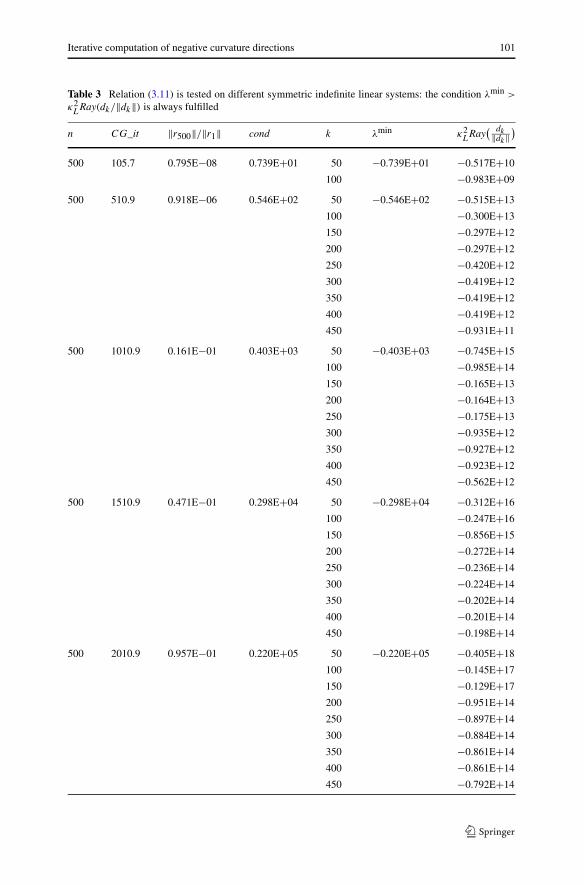
Iterative computation of negative curvature directions 101
Table 3 Relation (3.11) is tested on different symmetric indefinite linear systems: the condition λmin >
κ2L
Ray(dk/‖dk‖) is always fulfilled
n CG_it ‖r500‖/‖r1‖ cond k λmin κ2L
Ray( dk‖dk‖
)
500 105.7 0.795E−08 0.739E+01 50 −0.739E+01 −0.517E+10
100 −0.983E+09
500 510.9 0.918E−06 0.546E+02 50 −0.546E+02 −0.515E+13
100 −0.300E+13
150 −0.297E+12
200 −0.297E+12
250 −0.420E+12
300 −0.419E+12
350 −0.419E+12
400 −0.419E+12
450 −0.931E+11
500 1010.9 0.161E−01 0.403E+03 50 −0.403E+03 −0.745E+15
100 −0.985E+14
150 −0.165E+13
200 −0.164E+13
250 −0.175E+13
300 −0.935E+12
350 −0.927E+12
400 −0.923E+12
450 −0.562E+12
500 1510.9 0.471E−01 0.298E+04 50 −0.298E+04 −0.312E+16
100 −0.247E+16
150 −0.856E+15
200 −0.272E+14
250 −0.236E+14
300 −0.224E+14
350 −0.202E+14
400 −0.201E+14
450 −0.198E+14
500 2010.9 0.957E−01 0.220E+05 50 −0.220E+05 −0.405E+18
100 −0.145E+17
150 −0.129E+17
200 −0.951E+14
250 −0.897E+14
300 −0.884E+14
350 −0.861E+14
400 −0.861E+14
450 −0.792E+14

102 G. Fasano, M. Roma
required to store n Lanczos vectors to ensure the convergence to second order criticalpoints. Actually, due to the requirement of limited storage room, only a (fixed) smallnumber of such vectors (say 50) is stored in practice.
We considered the monotone version (MonNC) of the method proposed in [19]where we replaced the computation of the negative curvature direction with the it-erative scheme proposed in Table 2. Therefore the resulting algorithm uses substan-tially the same Newton-type direction as in the MonNC algorithm, and differs fromMonNC only in the determination of the negative curvature direction. This is moti-vated by the need to assess only the new iterative scheme for computing the direc-tion of negative curvature, the computation of the Newton direction being equal (ofcourse, a more realistic algorithm could be considered, which uses the same itera-tive scheme for computing both the search directions). As regards all the parameters,we adopt the standard values reported in [19], while as termination criterion we use‖∇f (xj )‖ ≤ 10−5 max{1,‖xj‖}.
The large scale unconstrained problems from the CUTEr collection [16] are usedas test problems. We compare the results obtained by the original (Lanczos based)MonNC truncated algorithm and the one which uses the new iterative scheme (weremark that for each outer iteration of the truncated scheme, both the algorithms areforced to perform the same number of inner iterations). In Table 4, we report the re-
Table 4 Comparison on nonconvex large scale problems, between the Lanczos based iterative scheme(MonNC [19]), and a Truncated Newton method which uses the algorithm in Table 1
Problem n Lanczos-based scheme New iterative scheme
it/ng nf it/ng nf
BRYBND 10000 26 42 25 34
COSINE 10000 10 15 9 13
CURLY10 10000 3034 3042 2963 2971
DIXMAANE 1500 15 17 15 17
DIXMAANE 3000 16 18 16 18
DIXMAANG 3000 15 16 15 16
DIXMAANH 1500 16 17 16 17
DIXMAANI 1500 24 25 24 25
DIXMAANI 3000 27 28 27 28
FLETCHCR 1000 1604 2368 1613 2417
GENROSE 1000 660 1194 679 1151
GENROSE 10000 6782 12380 6916 11693
MSQRTALS 1024 49 50 46 47
MSQRTBLS 1024 45 46 45 46
SINQUAD 1000 17 24 19 24
SINQUAD 10000 27 35 31 39
SPMSRTLS 1000 15 16 15 16
SPMSRTLS 10000 18 19 18 19
TOINTGSS 1000 5 6 6 7
TOINTGSS 10000 5 6 5 6
WOODS 1000 65 95 56 71
WOODS 10000 109 123 107 129

Iterative computation of negative curvature directions 103
sults obtained for all the problems coherently solved by both the algorithms, whereconvergence to the same point is achieved and negative curvature directions were en-countered (if negative curvature directions are not encountered, the two algorithmscoincide). The results are reported in terms of number of iterations and gradient eval-uations (it/ng), number of function evaluations (nf). We highlight that this preliminarytest does not aim at assessing the performance of two different algorithms; rather ittests the new approach in computing negative curvature directions in optimizationframeworks. From these results it can be observed that the adoption of the iterativescheme based on the FLR algorithm provides “good” directions of negative curvature.In fact, our proposal is effective and, in some cases, even better than the Lanczosbased scheme MonNC. Moreover, unlike algorithm MonNC, we recall that the newscheme does not require to store any matrix, in order to guarantee the convergence tosecond order critical points.
5 Conclusions
In this paper we introduce a new approach for iteratively computing directions of neg-ative curvature, for an indefinite matrix. The latter result can be used within differentcontexts of large scale optimization. The aim of this work is to provide a generaltheoretical framework to ensure the convergence to second order critical points, insolving optimization problems. The resulting method allows to compute adequatenegative curvature directions, avoiding any matrix storage in large scale settings. Weperformed a preliminary numerical experience where our proposal was effective.
However, to better evaluate the efficiency of the proposed method, an extensive nu-merical testing is certainly needed, and this deserves a separate work. In fact, a wideinvestigation is necessary on different optimization contexts, in order to assess thecapability of our approach to take advantage from the nonconvexity of the objectivefunction.
Acknowledgement This work was partially supported by the Ministero delle Infrastrutture e deiTrasporti in the framework of the research plan “Programma di Ricerca sulla Sicurezza,” Decreto17/04/2003 G.U. n. 123 del 29/05/2003. This work was also partially supported by Research Project FIRBRBNE01WBBB on “Large Scale Nonlinear Optimization,” Rome, Italy.
We would like to thank the anonymous referee for the constructive comments and suggestions whichled to improve the paper.
References
1. Bank, R., Chan, T.: A composite step bi-conjugate gradient algorithm for nonsymmetric linear sys-tems. Numer. Algorithms 7, 1–16 (1994)
2. Boman, E., Murray, W.: An iterative approach to computing a direction of negative curvature. Pre-sented at Copper Mountain conference, March 1998. Available at the url: www-sccm.stanford.edu/students/boman/papers.shtml
3. Conn, A.R., Gould, N.I.M., Toint, P.L.: Trust-Region Methods. MPS–SIAM Series on Optimization.SIAM, Philadelphia (2000)
4. Cullum, J., Willoughby, R.: Lanczos Algorithms for Large Symmetric Eigenvalue Computations.Birkhäuser, Boston (1985)
5. Dixon, L., Ducksbury, P., Singh, P.: A new three-term conjugate gradient method. Technical report130, Numerical Optimization Centre, Hatfield Polytechnic, Hatfield, Hertfordshire, UK (1985)

104 G. Fasano, M. Roma
6. Facchinei, F., Lucidi, S.: Convergence to second order stationary points in inequality constrainedoptimization. Math. Oper. Res. 93, 746–766 (1998)
7. Fasano, G.: Use of conjugate directions inside Newton-type algorithms for large scale unconstrainedoptimization. PhD thesis, Università di Roma “La Sapienza”, Roma, Italy (2001)
8. Fasano, G.: Lanczos-conjugate gradient method and pseudoinverse computation, on indefinite andsingular systems. J. Optim. Theory Appl. DOI 10.1007/s10957-006-91193
9. Fasano, G.: Planar-conjugate gradient algorithm for large-scale unconstrained optimization, part 1:theory. J. Optim. Theory Appl. 125, 523–541 (2005)
10. Fasano, G.: Planar-conjugate gradient algorithm for large-scale unconstrained optimization, part 2:application. J. Optim. Theory Appl. 125, 543–558 (2005)
11. Fasano, G., Roma, M.: Iterative computation of negative curvature directions in large scale optimiza-tion: theory and preliminary numerical results, Technical report 12-05, Dipartimento di Informaticae Sistemistica “A. Ruberti”, Roma, Italy (2005)
12. Ferris, M., Lucidi, S., Roma, M.: Nonmonotone curvilinear linesearch methods for unconstrainedoptimization. Comput. Optim. Appl. 6, 117–136 (1996)
13. Golub, G., Van Loan, C.: Matrix Computations, 3rd edn. John Hopkins University Press, Baltimore(1996).
14. Gould, N.I.M., Lucidi, S., Roma, M., Toint, P.L.: Solving the trust-region subproblem using the Lanc-zos method. SIAM J. Optim. 9, 504–525 (1999)
15. Gould, N.I.M., Lucidi, S., Roma, M., Toint, P.L.: Exploiting negative curvature directions in linesearchmethods for unconstrained optimization. Optim. Methods Softw. 14, 75–98 (2000)
16. Gould, N.I.M., Orban, D., Toint, P.: CUTEr (and SifDec), a constrained and unconstrained testingenvironment, revisited. ACM Trans. Math. Softw. 29, 373–394 (2003)
17. Hestenes, M.: Conjugate Direction Methods in Optimization. Springer, New York (1980)18. Liu, Y., Storey, C.: Efficient generalized conjugate gradient algorithm, part 1. J. Optim. Theory Appl.
69, 129–137 (1991)19. Lucidi, S., Rochetich, F., Roma, M.: Curvilinear stabilization techniques for truncated Newton meth-
ods in large scale unconstrained optimization. SIAM J. Optim. 8, 916–939 (1998)20. Lucidi, S., Roma, M.: Numerical experiences with new truncated Newton methods in large scale
unconstrained optimization. Comput. Optim. Appl. 7, 71–87 (1997)21. McCormick, G.: A modification of Armijo’s step-size rule for negative curvature. Math. Program. 13,
111–115 (1977)22. Miele, A., Cantrell, J.: Study on a memory gradient method for the minimization of functions. J. Op-
tim. Theory Appl. 3, 459–470 (1969)23. Moré, J., Sorensen, D.: On the use of directions of negative curvature in a modified Newton method.
Math. Program. 16, 1–20 (1979)24. Moré, J., Sorensen, D.: Computing a trust region step. SIAM J. Sci. Stat. Comput. 4, 553–572 (1983)25. Nash, S.: A survey of truncated-Newton methods. J. Comput. Appl. Math. 124, 45–59 (2000)26. Paige, C., Saunders, M.: Solution of sparse indefinite systems of linear equations. SIAM J. Numer.
Anal. 12, 617–629 (1975)27. Parlett, B.: The Symmetric Eigenvalue Problem. Prentice-Hall Series in Computational Mathematics.
Prentice-Hall, Englewood Cliffs (1980)28. Shultz, G., Schnabel, R., Byrd, R.: A family of trust-region-based algorithms for unconstrained mini-
mization. SIAM J. Numer. Anal. 22, 47–67 (1985)29. Stoer, J.: Solution of large linear systems of equations by conjugate gradient type methods. In:
Bachem A., Grötschel M., Korte B. (eds.) Mathematical Programming. The State of the Art, pp. 540–565. Springer, Berlin/Heidelberg (1983)
30. Trefethen, L., Bau, D.: Numerical Linear Algebra. SIAM, Philadelphia (1997)