Iterative Basis Pursuit for Image Sequence...

Iterative Basis Pursuit for Image Sequence Denoising Brian Eriksson ECE 738 Final Project Abstract An iterative method is purposed in this paper using the basis pursuit algorithm for spatial denoising, coupled with temporal wavelet denoising to result in a denoised video signal. Introduction Several new techniques have been developed recently for the purposes of denoising images. The most promising of these techniques have been the curvelet and undecimated wavelet transforms. Using a basis pursuit algorithm, the advantages of each algorithm can be taken advantage of to produce a spatially denoised image. When working with image sequences, the correlation between frames can be used to denoise images. Considering each pixel as a time-domain signal across multiple frames, this signal can be denoised using hard thresholding of wavelets. This paper purposes a iterative method of basis pursuit spatial denoising combined with temporal denoising using wavelets to produce a denoised image sequence signal. Curvelet Algorithm The Curvelet transform (original purposed in [4]) consists of an overcomplete representation of an image using a series of L2 energy measurements ranging across scale, orientation, and position. Each curvelet consists of a tight frame constrained over a slice of the fourier domain. In the spatial domain, the curvelet is a scaled and rotated gabor signal along the width and is a scaled and rotated gaussian signal along the length. One of the most important properties of the curvelet is length = width^2 (length = 2^-J, width = 2^-(2*J), J = scale). This allows for the curvelet to act like a needle at fine scale representations. A brief overview of the mathematical framework from [2] is now presented to give the reader a formal representation of curvelets. Each curvelet is defined by three parameters (J, K, L). J = Scale L = orientation K = location

Brian Eriksson – Iterative Basis Pursuit for Image Sequence Denoising 2

Parabolic Scaling Matrix:

⎟⎟⎠

⎞⎜⎜⎝

⎛=

J

j

JD 20022

Rotation Angle:

lJJ *2*2 −= πθ

Translation Parameter:

1 1 2 2

1 2

( * , * ), _ tan

k k knormalizing cons ts

δ δ δδ δ

=

=

Curvelet Basis Function:

1 2 1 2

1 1

2 2

( , ) ( ) * ( )( ) ( )( ) ( )

x x x xx Gabor xx Gaussian x

γ ψ ϕψϕ

===

Finally, the curvelet parameterized by (J,K,L) can be defined as 32

( , , ) 1 2 1 2( , ) 2 * ( * * ( , ) )J

j

j l k Jx x D R x x kθ δγ γ= − Curvelet Properties: -Anisotropy Scaling Law 2lengthwidth ≈ -Directional Sensitivity

JnsOrientatioof 1__# =

-Spatial Localization -Curvelet coefficients form a Cartesian coordinate grid with spacing

proportional to the length in Jθ direction and the width of the

curvelet in the normal (respective to Jθ ) direction. -Oscillatory Nature

-Across a ridge, a curve displays an oscillatory nature. This is shown by the use of the gabor waveform in the normal direction.


Now a more intuitive graphical explaination of the curvelet transform is presented. (Spatial Domain) (Curvelet Coefficient Domain) Figure – Example of a group of curvelets at a fixed orientation and scale and its relationship to the curvelet transform. Each coefficient relates to an L2 energy measurement of the oval region in the spatial domain. Figure – Example of curvelets with fixed scale and location, varying along orientation Using curvelets of varying orientation (figure above) the resulting coefficients would be very close to zero for (A) due to only a small amount of edge energy included in the curvelet area. (B) would have a slightly larger coefficient but still relatively small in comparison to the coefficient related to figure (C) which would be quite large due to the tight frame of the curvelet being tangential to the edge.

(A) (B) (C)


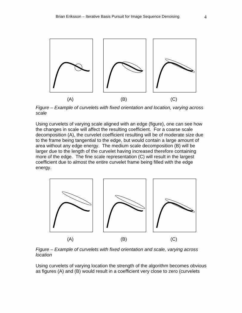
Figure – Example of curvelets with fixed orientation and location, varying across scale Using curvelets of varying scale aligned with an edge (figure), one can see how the changes in scale will affect the resulting coefficient. For a coarse scale decomposition (A), the curvelet coefficient resulting will be of moderate size due to the frame being tangential to the edge, but would contain a large amount of area without any edge energy. The medium scale decomposition (B) will be larger due to the length of the curvelet having increased therefore containing more of the edge. The fine scale representation (C) will result in the largest coefficient due to almost the entire curvelet frame being filled with the edge energy. Figure – Example of curvelets with fixed orientation and scale, varying across location Using curvelets of varying location the strength of the algorithm becomes obvious as figures (A) and (B) would result in a coefficient very close to zero (curvelets

(A) (B) (C)

(A) (B) (C)


are not compactly supported), while the coefficient related to (C) would be very large due to the edge being contained in the curvelet frame. In [1] it is shown that curvelets give a sparse representation of edges in C2 space. The problem with curvelets is their poor presentation of point singularities, which relates to points or corners in an image. This is shown at length in [2], as using the curvelet transform to reconstruct a noisy version of the Lena image results in very high quality performance on the elongated potions of the image (hat edges, outline of lena’s face), but performs quite poorly on the fine scale edges (eyes, mouth). Undecimated Wavelet Algorithm The standard one-dimensional A Trous Wavelet filter structure has the appearance of: Figure - Analysis Phase Figure - Synthesis Phase This is the structure that is used when a normal orthogonal discrete wavelet transform is performed.

HPF

LPF

2

2 HPF

LPF

2

2 HPF

LPF

2

2

2

2

HPF

LPF

+

2

2

HPF

LPF

+

2

2

HPF

LPF

+


The undecimated wavelet transform is performed by removing all the upsampling and downsampling blocks from the filter bank. In this representation, the signal is never decimated (downsampled), so the wavelet coefficients at each level are the same size as the original signal. This is a change from the critically sampled orthogonal wavelet transform, where the size of the coefficients after filtering is the same size of the original image. For an image transformed under the Undecimated Discrete Wavelet Transform (UDWT), decomposition and reconstruction under one level would have the filter bank representation of: Figure – Undecimated Wavelet Transform It should be noted that after one level of analysis, the size of the wavelet coefficients would be 4 times larger than the original image size. Like Orthogonal wavelets, the Undecimated wavelet transform will obtain a sparse representation of singularities (corners in an image) while performing quite poorly on the elongated portions (long edges). This is shown in detail in [2], as the reconstruction of the noisy Lena image results in very good performance in the fine detail edges (facial features), while doing quite poorly on the long edges (outline of Lena, hat edges).

LPF Rows

HPF Rows

LPF Cols

HPF Cols

HPF Cols

LPF Cols

LPF Cols

HPF Cols

HPF Cols

LPF Cols

LPF Rows

HPF Rows


Basis Pursuit Method Currently we have presented the curvelet method that works well for long curves but poorly for sharp edges, and the undecimated wavelet method that works well for sharp edges but poorly for long curves. Intuitively, one would want to use what the both methods do well, and leave out what they do poorly. This is the intention of the Basis Pursuit method. A generalized method of basis pursuit is described in [2], below is the modified version implemented in this paper.

imagenoisysTransformCurveletInverseT

TransformCurveletTTransformWaveletdUndecimateInverseT

TransformWaveletdUndecimateT

curve

curve

wave

wave

___

____

__

1

1

==

==

=

−

−

iterations1

1

=

=

δ

λ

imagezerousT

sT

curveNoise

curve

waveNoise

wave

_)(

)(

==

=

α

α

noisestdtvalsignificannoisestderrorval

_*2_=

=

for k = 1:iterations

waveNoise

wavewave

wavewave

residual

uT

αα

α

−=

= )(

if errorvaljkresidualwave >),( & tvalsignificanjkNoisewave >),(α

),(),( jkjk Noisewavewave αα =

)),,((_),( λαα jkthresholdsoftjk wavewave = End

)(1wavewaveTu α−=


curve

Noisecurvecurve

curvecurve

residual

uT

αα

α

−=

= )(

if errorvaljkresidualcurve >),( & tvalsignificanjkNoisecurve >),(α

),(),( jkjk Noisecurvecurve αα =

)),,((_),( λαα jkthresholdsoftjk curvecurve = end

)(1curvecurveTu α−=

)(__ uvaluesnegativeclipu = δλλ −= end The ideal results of this algorithm would be an image that reconstructs the long edges of an image like the curvelet transform, while reconstructing the sharp edges like the undecimated wavelet transform. Temporal Wavelet Algorithm With an image sequence, there is structured redundancy across multiple frames. This redundancy can be related to the background or a slow moving object. Ideally we would want to average the background pixels and modify them to values as constant as possible while still allowing each pixel to change for movement. (A)


(B) Figure – Pixel observed across a group of frames The peaks of the pixel value graph are assumed to be the result of motion in the image, all other values are assumed to be background that is under the effect of noise. Using a standard (decimated/orthogonal) haar wavelet transform, the pixel graph is denoised using hard thresholding. All coefficients below a certain range (value determined by the noise model) are thresholded to zero. The result should appear like the graph below. Figure – Wavelet denoised pixel signal Ideally the result of this method would be background pixels averaged out across all frames, while pixels that are the result of motion would be maintained at their original value.

Frame Number

Pix

el V

alue

Frame Number

Pix

el V

alue


Iterative Basis Pursuit Algorithm Description An iterative method is now purposed using both basis pursuit and the temporal wavelet method. Prior to this algorithm, the groups of frames are denoised using a light wiener filter and block averaging. original_frames = Noisy group of frames std = standard deviation of additive noise

_ _ _ ( _ )_ _ _ ( _ )

_ _ _ lg ( _ , )_ [0.3* , 0.15* , 0.075* ]

wiener frames Light Wiener Filter original framesblock frames Block Averaging Filter wiener framesnew frames Basis Persuit A oirhtm block frames stdstd array std std std

==

==

For 3:1=k

_ ( )_ _ _ lg ( _ ,3* )

_ _ _ lg ( _ ,1.2* )

std std array kbasis frames Basis Pursuit a orithm new frames stdnew frames Temporal Wavelet a orithm basis frames std

===

End

Noisy Image

Base

Basis PursuitTemporal

Denoised

Update

Noisy Image

Base Denoising Techniques

Basis PursuitTemporal

Update Assumed

Noise

Basis Pursuit

Temporal Wavelet Denoising

Denoised Image


The idea behind this is that basis pursuit denoising will reconstruct the frame image while also reconstructing some of the noise. The temporal wavelet denoising technique is very good at removing noise in redundant pixels, but will add its own noise caused by movement in the image. By iterating multiple times and decreasing the amount of assumed noising each time, the movement noise caused by the temporal wavelet denoising will be removed by the basis pursuit algorithm and a majority of the noise reconstructed by basis pursuit will be eliminated by temporal wavelets. Experiments The iterative basis pursuit method was tested using two image sequence sets. One set, the MOBCAL sequence, consists a real video sequence with many different objects moving simultaneously. The other set, the cartoon sequence, is a series of drawings with a large amount of constant background with characters running across the screen. The sequences were tested using a light noise condition (variance = 100) and a heavy noise condition (variance = 900). Results After examining the preliminary results it was determined that the interesting cases were the MOBCAL sequence under light noise and the CARTOON sequence under heavy noise. The first results received were very optimistic for the heavy noise cases, with iterative method PSNR performing almost 1 dB better than all other methods. The light noise case showed a significantly different story as the iterative basis pursuit method was far too drastic with its denoising and ended up blurring the image. The resulting PSNR values were more than 1 dB away from the best method for this case (the base denoising methods). These observations were taken into consideration and the iterative method’s threshold values were modified in order to even up the performance results.


Figure: MOBCAL Sequence with additive noise standard deviation = 10. (Plus sign) = Iterative Basis Pursuit Method, (Circle) = Single Basis Pursuit, (Square) = Curvelet Denoising, (Diamond) = Base Denoising methods As shown in the figure, the iterative basis pursuit method still performs below the base denoising methods in this case. After modifying the method, the results improved from 1 dB away to only roughly 0.4 dB away from the best denoising method.

Figure: (A) The original frame image, (B) Frame image after additive white noise


Figure: (A) Frame denoised using Basis Pursuit spatial method, (B) Frame denoised using Curvelet denoising, (C) Frame denoised after iterative basis pursuit method From a distance the iterative basis pursuit method appears to perform the best out of all three methods. In the iterative basis image all the smooth areas appear to be completely denoised with very little variation along smooth patches.


Figure: (A) Frame denoised using Basis Pursuit spatial method, (B) Frame denoised using Curvelet denoising, (C) Frame denoised after iterative basis pursuit method Upon zooming in on an area containing a majority of smooth areas, the power of both basis pursuit methods (A,C) can be seen. Specifically compare the noise contained on the surface of the ball and on the edge of the calendar between the basis pursuit methods (A,C) and the curvelet denoising method (B). By comparing the dark sections of the wall, the difference between the spatial basis pursuit (A) and the iterative basis pursuit method (C) can be seen.


Figure: (A) Frame denoised using Basis Pursuit spatial method, (B) Frame denoised using Curvelet denoising, (C) Frame denoised after iterative basis pursuit method The failure of the iterative method can be seen in the figure above. Notice the detail of the pigs on the wallpaper in the curvelet denoised method (B). Now contrast again the iterative denoised image in (C). Although the method does fairly well in denoising the smooth portions of the wallpaper, the details on the pigs is almost completely eliminated. This causes the drop in PSNR for the iterative basis pursuit method.


Figure: Cartoon Sequence with additive noise standard deviation = 30. (Plus sign) = Iterative Basis Pursuit Method, (Circle) = Single Basis Pursuit, (Square) = Curvelet Denoising, (Diamond) = Base Denoising methods The PSNR resulting from denoising the CARTOON sequence plot is seen above. The iterative basis pursuit performs by far the best for this image sequence. This can be explained because the CARTOON image sequence consists of a large number of smooth image portions which the iterative basis pursuit method can denoise quite well.

Figure: (A) Frame image of original CARTOON sequence, (B) Frame image of CARTOON sequence with additive noise with variance = 900


Figure: (A) Frame denoised using Basis Pursuit spatial method, (B) Frame denoised using Curvelet denoising, (C) Frame denoised after iterative basis pursuit method The advantages of the iterative basis pursuit method can be seen in the figure above. By cursorily glance, one can see that the background in (C) contains drastically less noise than the images (A) or (B). In contrast, the areas around the lion (which is quick motion in the image sequence) contain some motion noise caused by the temporal wavelet denoising techniques, as expected this noise does not appear in the other two images.


Figure: (A) Frame denoised using Basis Pursuit spatial method, (B) Frame denoised using Curvelet denoising, (C) Frame denoised after iterative basis pursuit method The failure of curvelets can be seen in image (A), as the fine detailed corners in the lion’s face (the eye, teeth) are very poorly represented after curvelet reconstruction. The improvements made by implementing basis pursuit can be seen in (B) as the eye and nose areas are much better defined by reconstructing with both curvelets and undecimated wavelets. The iterative basis pursuit image (C) shows both improvements and problems over the previous methods. The fine detail seems to be better defined that the single basis pursuit methods, while motion noise caused by temporal wavelets seems to drastically degrade the image.


Conclusions As can be seen in the two experiments detailed in this paper, the iterative basis pursuit method has both advantages and drawbacks. In light noise situations, results can be assumed to be comparable or slightly below established denoising methods. In heavy noise situations, the iterative method outperforms all other methods tested. The smooth areas of the image that remain stationary across multiple frames will result in very high denoising performance while problems exist with fast motion causing less than ideal temporal wavelet denoising results. References [1] - E. J. Candès and D. L. Donoho (2004), New Tight Frames of Curvelets and Optimal Representations of Objects and Piecewise C2 Singularities, Communications on Pure and Applied Mathematics, Vol. LVII, 219-266 [2] – J. L. Starck, E. J. Candès and D. L. Donoho (2001). Very High Quality Image Restoration by Combining Wavelets and Curvelets, Wavelet Applications in Signal and Image Processing IX, Proc. SPIE 4478 [3] - A Gyaourova, C Kamath, IK Fodor, Undecimated wavelet transforms for image denoising, Technical report, Lawrence Livermore National Laboratory [4] - E. J. Candès and D. L. Donoho (1999). Curvelets – A surprisingly effective nonadaptive representation for objects with edges. Curves and surfaces, 105-120 [5] – A. Kokaram, Motion Picture Restoration, Springer-Verlag 1998 Software References The Curvelet Transform was performed using a beta version of the MATLAB Curvelet Toolbox by Laurent Demanet - http://www.acm.caltech.edu/~demanet/ The Undecimated Wavelet Transform was performed using the Rice Wavelet Toolkit (RWT) - http://www.dsp.rice.edu/software/rwt.shtml Image sequences used were from “Motion Picture Restoration” - http://www.mee.tcd.ie/~ack/ All other code was developed by Brian Eriksson.

Iterative Basis Pursuit for Image Sequence...

Documents

Transcript of Iterative Basis Pursuit for Image Sequence...