Istituto Nazionale di AstrofisicaIstituto di Fisica dello Spazio Interplanetario Consiglio Nazionale...
72
Torino 4 – 7 September Torino 4 – 7 September 2006 2006 Istituto Nazionale di Astrofisica Istituto di Fisica dello Spazio Interplanetario Consiglio Nazionale delle Ricerche Istituto di Scienza e Tecnologie della Informazione David M. Lucchesi David M. Lucchesi The Lense–Thirring effect The Lense–Thirring effect measurement with LAGEOS measurement with LAGEOS satellites: satellites: David M. Lucchesi David M. Lucchesi 1,2,3 1,2,3 Error Budget and impact of the time– Error Budget and impact of the time– dependent part of Earth’s gravity dependent part of Earth’s gravity field field 1. Istituto di Fisica dello Spazio Interplanetario (IFSI/INAF), Roma, Italy 2. Istituto di Scienza e Tecnologie della Informazione (ISTI/CNR), Pisa, Italy 3. Istituto Nazionale di Fisica Nucleare (INFN), Sezione di Roma XVII SIGRAV Conference XVII SIGRAV Conference
-
Upload
britton-marsh -
Category
Documents
-
view
215 -
download
0
Transcript of Istituto Nazionale di AstrofisicaIstituto di Fisica dello Spazio Interplanetario Consiglio Nazionale...
Torino 4 – 7 September 2006Torino 4 – 7 September 2006
Istituto Nazionale di AstrofisicaIstituto di Fisica dello Spazio Interplanetario
Consiglio Nazionale delle RicercheIstituto di Scienza e Tecnologie della Informazione
David M. LucchesiDavid M. Lucchesi
The Lense–Thirring effect measurement The Lense–Thirring effect measurement with LAGEOS satellites:with LAGEOS satellites:
David M. LucchesiDavid M. Lucchesi 1,2,31,2,3
Error Budget and impact of the time–dependent Error Budget and impact of the time–dependent part of Earth’s gravity fieldpart of Earth’s gravity field
1. Istituto di Fisica dello Spazio Interplanetario (IFSI/INAF), Roma, Italy
2. Istituto di Scienza e Tecnologie della Informazione (ISTI/CNR), Pisa, Italy
3. Istituto Nazionale di Fisica Nucleare (INFN), Sezione di Roma II, Roma, Italy
XVII SIGRAV ConferenceXVII SIGRAV Conference
Torino 4 – 7 September 2006Torino 4 – 7 September 2006
David M. LucchesiDavid M. Lucchesi
Table of ContentsTable of Contents
Gravitomagnetism and Lense–Thirring effect;Gravitomagnetism and Lense–Thirring effect; The LAGEOS satellites and SLR;The LAGEOS satellites and SLR; The 2004 measurement and its error budget (EB);The 2004 measurement and its error budget (EB); The reviewed EB and the J-dot contribution;The reviewed EB and the J-dot contribution; Difficulties in improving the present measurement Difficulties in improving the present measurement
with LAGEOS satellites only;with LAGEOS satellites only; Conclusions;Conclusions;
Torino 4 – 7 September 2006Torino 4 – 7 September 2006
David M. LucchesiDavid M. Lucchesi
Gravitomagnetism and Lense–Thirring effectGravitomagnetism and Lense–Thirring effect
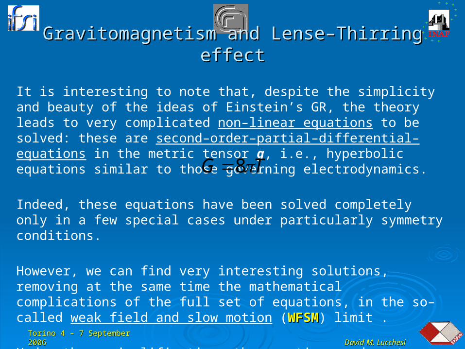
It is interesting to note that, despite the simplicity and beauty of the ideas of Einstein’s GR, the theory leads to very complicated non–linear equations to be solved: these are second–order–partial–differential–equations in the metric tensor g, i.e., hyperbolic equations similar to those governing electrodynamics.
Indeed, these equations have been solved completely only in a few special cases under particularly symmetry conditions.
However, we can find very interesting solutions, removing at the same time the mathematical complications of the full set of equations, in the so–called weak field and slow motion (WFSMWFSM) limit .
Under these simplifications the equations reduce to a form quite similar to those of electromagnetism.
TG
8
Torino 4 – 7 September 2006Torino 4 – 7 September 2006
David M. LucchesiDavid M. Lucchesi
Gravitomagnetism and Lense–Thirring effectGravitomagnetism and Lense–Thirring effect
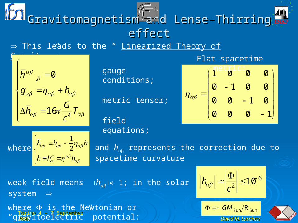
This leads to the “ Linearized Theory of Gravity ”:
Tc
Gh
hg
h
4
,
16
0 gauge conditions;
metric tensor;
field equations;
1000
0100
0010
0001
Flat spacetime metric:
and h represents the correction due to spacetime curvature
hhh
hhh2
1
where
weak field means h« 1; in the solar system 6
210
ch
where is the Newtonian or “gravitoelectric” potential: SunSun RGM
Torino 4 – 7 September 2006Torino 4 – 7 September 2006
David M. LucchesiDavid M. Lucchesi
Gravitomagnetism and Lense–Thirring effectGravitomagnetism and Lense–Thirring effect
Tc
Gh
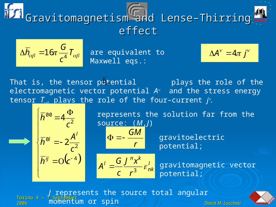
416 jA 4are equivalent to Maxwell eqs.:
That is, the tensor potential plays the role of the electromagnetic vector potential A and the stress energy tensor T plays the role of the four–current j.
4
20
200
2
4
ch
c
Ah
ch
ij
ll
represents the solution far from the source: (M,J)
r
GM gravitoelectric potential;
lnk
knl
r
xJ
c
GA
3 gravitomagnetic vector potential;
J represents the source total angular momentum or spin
h
Torino 4 – 7 September 2006Torino 4 – 7 September 2006
David M. LucchesiDavid M. Lucchesi
Gravitomagnetism and Lense–Thirring effectGravitomagnetism and Lense–Thirring effect
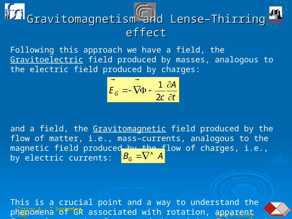
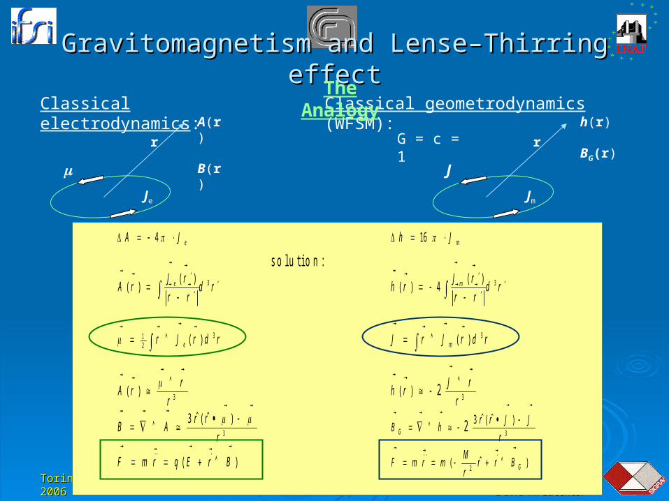
Following this approach we have a field, the Gravitoelectric field produced by masses, analogous to the electric field produced by charges:
and a field, the Gravitomagnetic field produced by the flow of matter, i.e., mass–currents, analogous to the magnetic field produced by the flow of charges, i.e., by electric currents:
This is a crucial point and a way to understand the phenomena of GR associated with rotation, apparent forces in rotating frames and the origin of inertia in general.
t
A
cEG
2
1
ABG
Torino 4 – 7 September 2006Torino 4 – 7 September 2006
David M. LucchesiDavid M. Lucchesi
Gravitomagnetism and Lense–Thirring effectGravitomagnetism and Lense–Thirring effect
These phenomena have been debated by scientists and philosophers since Galilei and Newton times.
In classical physics, Newton’s law of gravitation has a counterpart in Coulomb’s law of electrostatics, but it does not have any phenomenon formally analogous to magnetism.
On the contrary, Einstein’s theory of gravitation predicts that the force generated by an electric current, that is Ampère’s law of electromagnetism, should have a formal counterpart force generated by a mass–current.
Torino 4 – 7 September 2006Torino 4 – 7 September 2006
David M. LucchesiDavid M. Lucchesi
Gravitomagnetism and Lense–Thirring effectGravitomagnetism and Lense–Thirring effect
eJA
4 mJh
16
s o l u t i o n :
rdrr
rJrA e
3)()(
rdrr
rJrh m
3)(4)(
rdrJr e
321 )(
rdrJrJ m
3)(
3)(
r
rrA
32)(
r
rJrh
3
)ˆ(ˆ3
r
rrAB
3
)ˆ(ˆ32r
JJrrhB G
)(...
BrEqrmF
)ˆ(.
2
..
GBrrr
MmrmF
r
Je
A(r)
B(r) J
r
Jm
h(r)
BG(r)
Classical electrodynamics: Classical geometrodynamics (WFSM):The Analogy
G = c = 1
Torino 4 – 7 September 2006Torino 4 – 7 September 2006
David M. LucchesiDavid M. Lucchesi
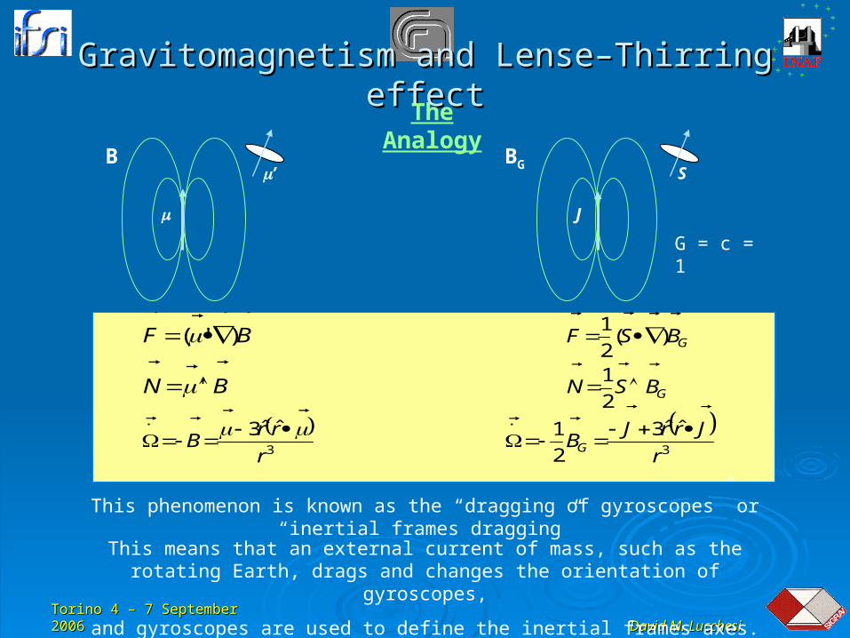
Gravitomagnetism and Lense–Thirring effectGravitomagnetism and Lense–Thirring effect
BF
)'( GBSF
)(2
1
BN
' GBSN
2
1
3
ˆˆ3
r
rrB
3
ˆˆ3
2
1
r
JrrJBG
B’
J
BGS
This phenomenon is known as the “dragging of gyroscopes” or “inertial frames dragging”
The Analogy
This means that an external current of mass, such as the rotating Earth, drags and changes the orientation of gyroscopes,
and gyroscopes are used to define the inertial frames axes.
G = c = 1
Torino 4 – 7 September 2006Torino 4 – 7 September 2006
David M. LucchesiDavid M. Lucchesi
Gravitomagnetism and Lense–Thirring effectGravitomagnetism and Lense–Thirring effect
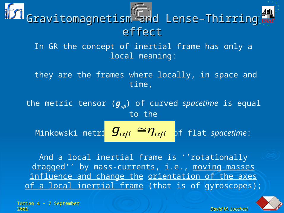
In GR the concept of inertial frame has only a local meaning:
they are the frames where locally, in space and time,
the metric tensor (g) of curved spacetime is equal to the
Minkowski metric tensor () of flat spacetime:
And a local inertial frame is ‘’rotationally dragged‘’ by mass-currents, i.e., moving masses influence and change the orientation
of the axes of a local inertial frame (that is of gyroscopes);
g
Torino 4 – 7 September 2006Torino 4 – 7 September 2006
David M. LucchesiDavid M. Lucchesi
Gravitomagnetism and Lense–Thirring effectGravitomagnetism and Lense–Thirring effect
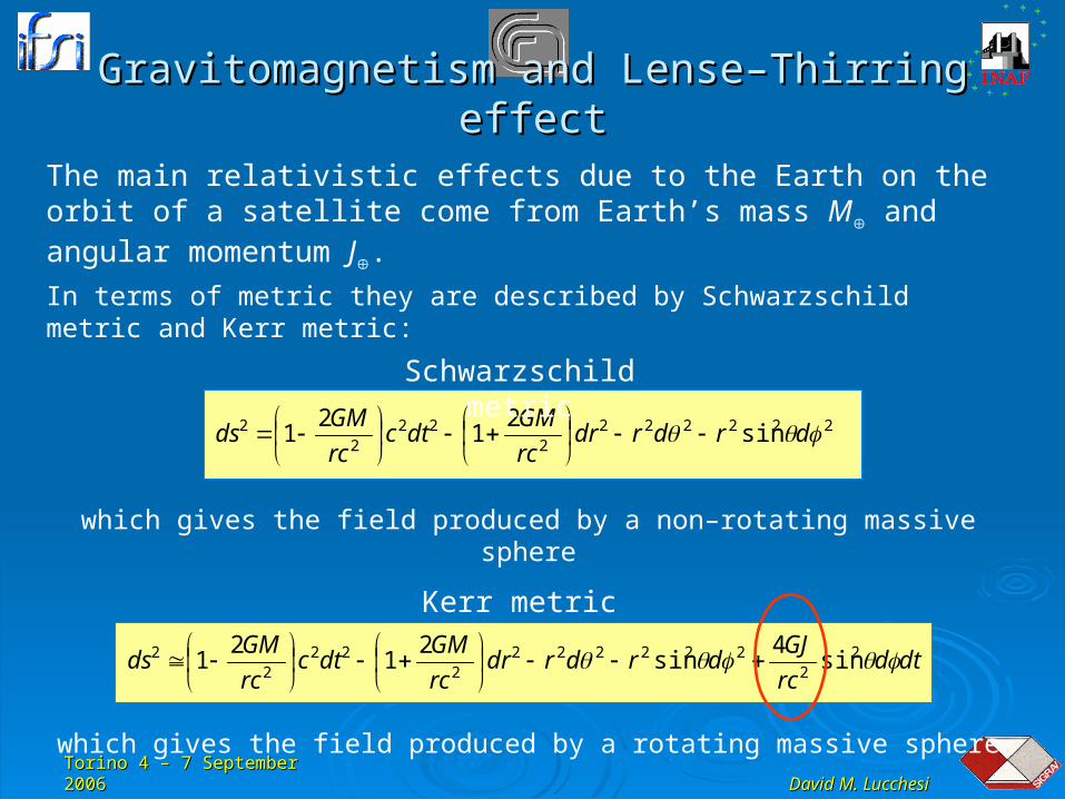
The main relativistic effects due to the Earth on the orbit of a satellite come from Earth’s mass M and angular momentum J.
2222222
222
2 sin2
12
1 drdrdrrc
GMdtc
rc
GMds
Schwarzschild metric
which gives the field produced by a non–rotating massive sphere
dtdrc
GJdrdrdr
rc
GMdtc
rc
GMds 2
2222222
222
22 sin
4sin
21
21
Kerr metric
which gives the field produced by a rotating massive sphere
In terms of metric they are described by Schwarzschild metric and Kerr metric:
Torino 4 – 7 September 2006Torino 4 – 7 September 2006
David M. LucchesiDavid M. Lucchesi
Gravitomagnetism and Lense–Thirring effectGravitomagnetism and Lense–Thirring effect
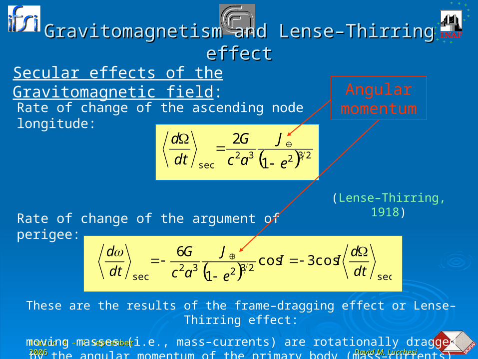
Secular effects of the Gravitomagnetic field:
23232sec 1
2
e
J
ac
G
dt
d
sec23232
sec
cos3cos1
6
dt
dII
e
J
ac
G
dt
d
Rate of change of the ascending node longitude:
Rate of change of the argument of perigee:
(Lense–Thirring, 1918)
Angular momentum
These are the results of the frame–dragging effect or Lense–Thirring effect:
moving masses (i.e., mass–currents) are rotationally dragged by the angular momentum of the primary body (mass–currents)
Torino 4 – 7 September 2006Torino 4 – 7 September 2006
David M. LucchesiDavid M. Lucchesi
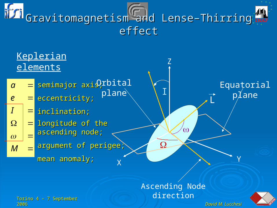
Keplerian elements
semimajor axis;semimajor axis;
eccentricity;eccentricity;
inclination;inclination;
M
I
e
a
longitude of the ascending node;longitude of the ascending node;
argument of perigee;argument of perigee;
mean anomaly;mean anomaly;
Orbital plane Equatorial plane
X Y
Z
LI
Ascending Node direction
Gravitomagnetism and Lense–Thirring effectGravitomagnetism and Lense–Thirring effect
Torino 4 – 7 September 2006Torino 4 – 7 September 2006
David M. LucchesiDavid M. Lucchesi
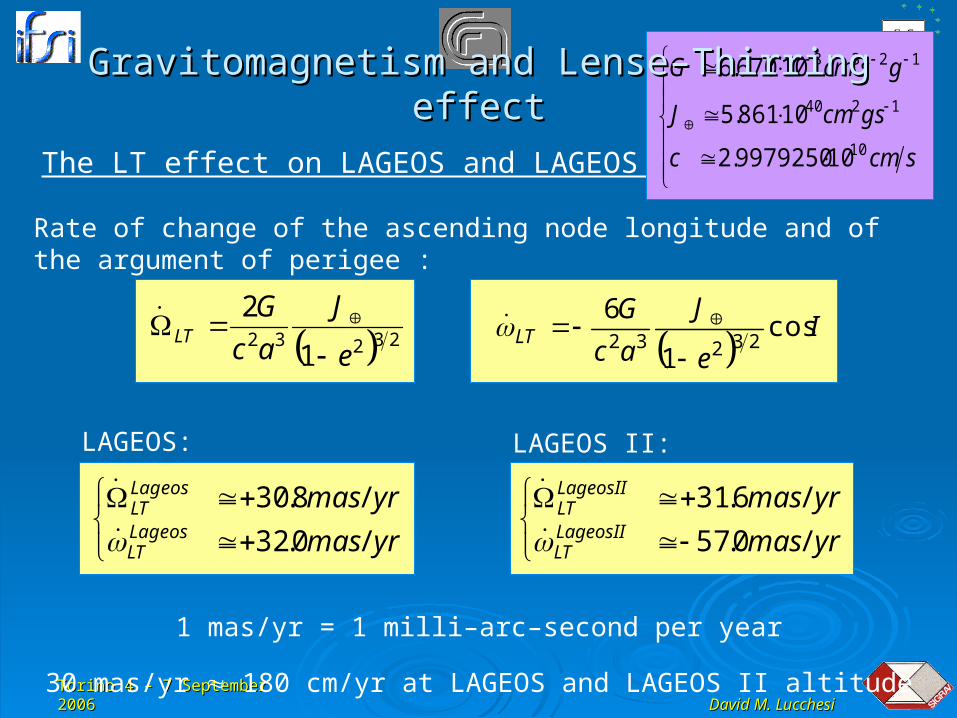
The LT effect on LAGEOS and LAGEOS II orbit
232321
2
e
J
ac
GLT
Ie
J
ac
GLT cos
1
623232
Rate of change of the ascending node longitude and of the argument of perigee :
LAGEOS:
yrmas
yrmasLageosLT
LageosLT
/0.32
/8.30
yrmas
yrmasLageosIILT
LageosIILT
/0.57
/6.31
LAGEOS II:
1 mas/yr = 1 milli–arc–second per year
30 mas/yr 180 cm/yr at LAGEOS and LAGEOS II altitude
scmc
gscmJ
gscmG
10
1240
1238
109979250.2
10861.5
10670.6Gravitomagnetism and Lense–Thirring effectGravitomagnetism and Lense–Thirring effect
Torino 4 – 7 September 2006Torino 4 – 7 September 2006
David M. LucchesiDavid M. Lucchesi
Table of ContentsTable of Contents
Gravitomagnetism and Lense–Thirring effect;Gravitomagnetism and Lense–Thirring effect; The LAGEOS satellites and SLR;The LAGEOS satellites and SLR; The 2004 measurement and its error budget (EB);The 2004 measurement and its error budget (EB); The reviewed EB and the J-dot contribution;The reviewed EB and the J-dot contribution; Difficulties in improving the present measurement Difficulties in improving the present measurement
with LAGEOS satellites only;with LAGEOS satellites only; Conclusions;Conclusions;
Torino 4 – 7 September 2006Torino 4 – 7 September 2006
David M. LucchesiDavid M. Lucchesi
The LAGEOS satellites and SLRThe LAGEOS satellites and SLR
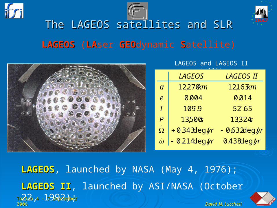
LAGEOS and LAGEOS II satellites
LAGEOSLAGEOS (LALAser GEOGEOdynamic SSatellite)
yryr
yryr
ssP
I
e
kmkma
IILAGEOSLAGEOS
deg/438.0deg/214.0
deg/632.0deg/343.0
324,13500,13
65.529.109
014.0004.0
163,12270,12
LAGEOSLAGEOS, launched by NASA (May 4, 1976);
LAGEOS IILAGEOS II, launched by ASI/NASA (October 22, 1992);
Torino 4 – 7 September 2006Torino 4 – 7 September 2006
David M. LucchesiDavid M. Lucchesi
The LAGEOS satellites and SLRThe LAGEOS satellites and SLR
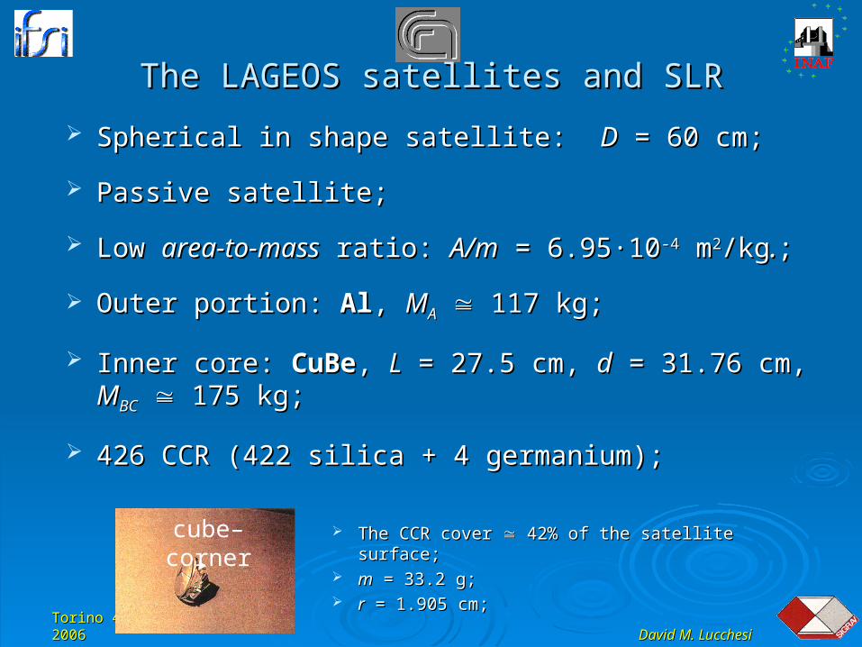
Spherical in shape satellite: Spherical in shape satellite: DD = 60 cm; = 60 cm;
Passive satellite;Passive satellite;
Low Low area-to-massarea-to-mass ratio: ratio: A/mA/m = 6.95·10 = 6.95·10-4-4 m m22/kg/kg..;;
Outer portion: Outer portion: AlAl, , MMAA 117 kg; 117 kg;
Inner core: Inner core: CuBeCuBe, , LL = 27.5 cm, = 27.5 cm, dd = 31.76 cm, = 31.76 cm, MMBCBC 175 175
kg;kg;
426 CCR (422 silica + 4 germanium);426 CCR (422 silica + 4 germanium);
cube–corner The CCR cover The CCR cover 42% of the satellite surface; 42% of the satellite surface; mm = 33.2 g; = 33.2 g; rr = 1.905 cm; = 1.905 cm;
Torino 4 – 7 September 2006Torino 4 – 7 September 2006
David M. LucchesiDavid M. Lucchesi
The LAGEOS satellites and SLRThe LAGEOS satellites and SLR
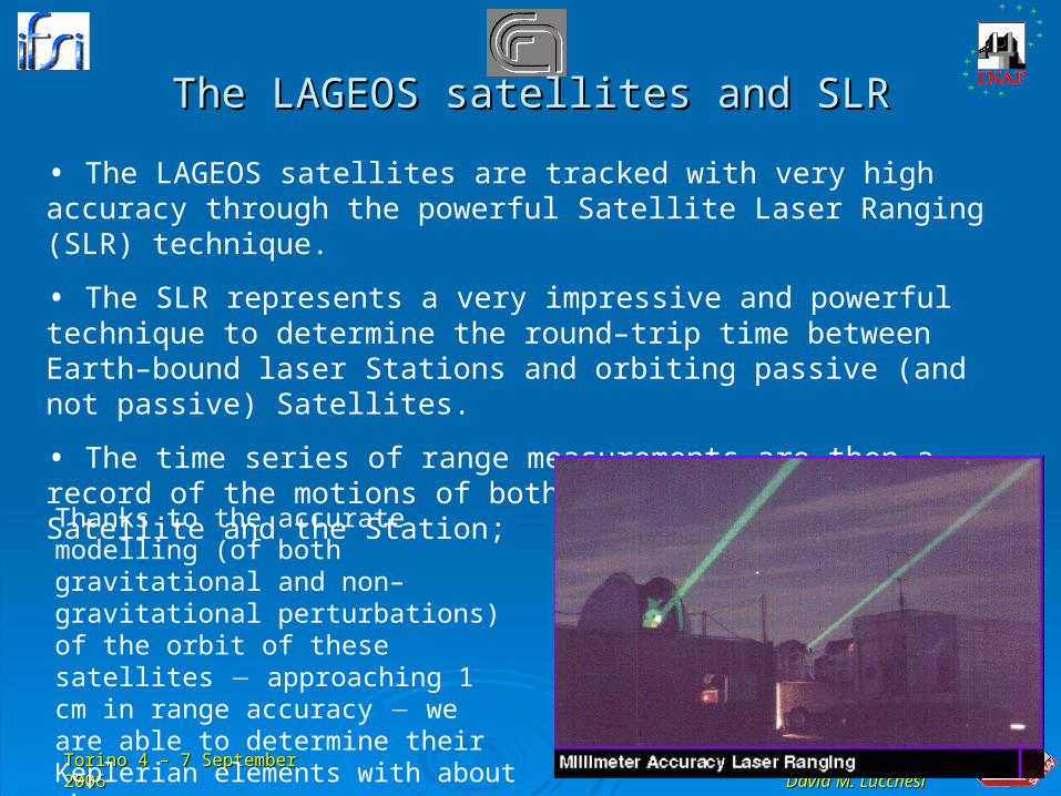
• The LAGEOS satellites are tracked with very high accuracy through the powerful Satellite Laser Ranging (SLR) technique.
• The SLR represents a very impressive and powerful technique to determine the round–trip time between Earth–bound laser Stations and orbiting passive (and not passive) Satellites.
• The time series of range measurements are then a record of the motions of both the end points: the Satellite and the Station;
Thanks to the accurate modelling (of both gravitational and non–gravitational perturbations) of the orbit of these satellites approaching 1 cm in range accuracy we are able to determine their Keplerian elements with about the same accuracy.
Torino 4 – 7 September 2006Torino 4 – 7 September 2006
David M. LucchesiDavid M. Lucchesi
The LAGEOS satellites and SLRThe LAGEOS satellites and SLR
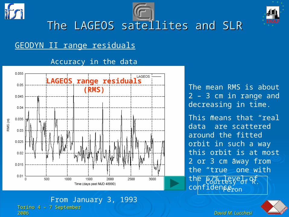
GEODYN II range residuals
Accuracy in the data reduction
From January 3, 1993
The mean RMS is about 2 – 3 cm in range and decreasing in time.
This means that “real data” are scattered around the fitted orbit in such a way this orbit is at most 2 or 3 cm away from the “true” one with the 67% level of confidence.
LAGEOS range residuals (RMS)
Courtesy of R. Peron

Torino 4 – 7 September 2006Torino 4 – 7 September 2006
David M. LucchesiDavid M. Lucchesi
The LAGEOS satellites and SLRThe LAGEOS satellites and SLR
• In this way the orbit of LAGEOS satellites may be considered as a reference frame, not bound to the planet, whose motion in the inertial space (after all perturbations have been properly modelled) is in principle known.
• Indeed, the normal points have typically precisions of a few mm, and accuracies of about 1 cm, limited by atmospheric effects and by variations in the absolute calibration of the instruments.
With respect to this external and quasi-inertial frame it is then possible to measure the absolute positions and motions of the ground–based stations, with an absolute accuracy of a few mm and mm/yr.
Torino 4 – 7 September 2006Torino 4 – 7 September 2006
David M. LucchesiDavid M. Lucchesi
The LAGEOS satellites and SLRThe LAGEOS satellites and SLR
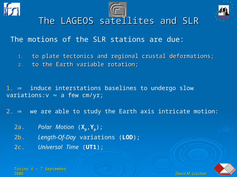
The motions of the SLR stations are due:
1.1. to plate tectonics and regional crustal deformations;to plate tectonics and regional crustal deformations;
2.2. to the Earth variable rotation;to the Earth variable rotation;
1. induce interstations baselines to undergo slow variations:v a few cm/yr;
2. we are able to study the Earth axis intricate motion:
2a. Polar Motion (Xp,Yp);
2b. Length-Of-Day variations (LOD);
2c. Universal Time (UT1);
Torino 4 – 7 September 2006Torino 4 – 7 September 2006
David M. LucchesiDavid M. Lucchesi
The LAGEOS satellites and SLRThe LAGEOS satellites and SLR
Dynamic effects of Geometrodynamics
Today, the relativistic corrections (both of Special and General relativity) are an essential aspect of (dirty) – Celestial Mechanics as well as of the electromagnetic propagation in space:
1. these corrections are included in the orbit determination–and–analysis programs for Earth’s satellites and interplanetary probes;
2. these corrections are necessary for spacecraft navigation and GPS satellites;
3. these corrections are necessary for refined studies in the field of geodesy and geodynamics;
Torino 4 – 7 September 2006Torino 4 – 7 September 2006
David M. LucchesiDavid M. Lucchesi
Table of ContentsTable of Contents
Gravitomagnetism and Lense–Thirring effect;Gravitomagnetism and Lense–Thirring effect; The LAGEOS satellites and SLR;The LAGEOS satellites and SLR; The 2004 measurement and its error budget (EB);The 2004 measurement and its error budget (EB); The reviewed EB and the J-dot contribution;The reviewed EB and the J-dot contribution; Difficulties in improving the present measurement Difficulties in improving the present measurement
with LAGEOS satellites only;with LAGEOS satellites only; Conclusions;Conclusions;
Torino 4 – 7 September 2006Torino 4 – 7 September 2006
David M. LucchesiDavid M. Lucchesi
The 2004 measurement and its error budgetThe 2004 measurement and its error budget
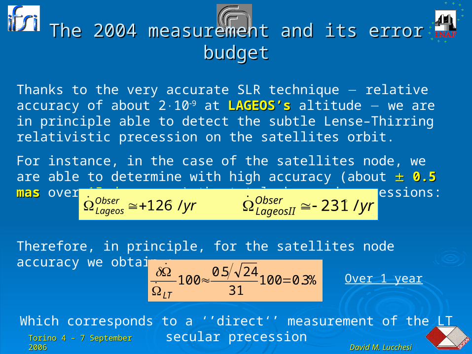
Thanks to the very accurate SLR technique relative accuracy of about 2109 at LAGEOS’sLAGEOS’s altitude we are in principle able to detect the subtle Lense–Thirring relativistic precession on the satellites orbit.
For instance, in the case of the satellites node, we are able to determine with high accuracy (about 0.5 mas 0.5 mas over 15 days arcs) the total observed precessions:
Therefore, in principle, for the satellites node accuracy we obtain :
yrObserLageos /126 yrObser
LageosII /231
%3.010031
245.0100
LT
Which corresponds to a ‘’direct‘’ measurement of the LT secular precession
Over 1 year
Torino 4 – 7 September 2006Torino 4 – 7 September 2006
David M. LucchesiDavid M. Lucchesi
The 2004 measurement and its error budgetThe 2004 measurement and its error budget
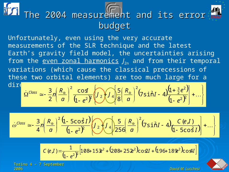
Unfortunately, even using the very accurate measurements of the SLR technique and the latest Earth’s gravity field model, the uncertainties arising from the even zonal harmonics J2n and from their temporal variations (which cause the classical precessions of these two orbital elements) are too much large for a direct measurement of the Lense–Thirring effect.
22
223
22
4222
2
1
14sin7
8
5
1
cos
2
3
e
eI
a
RJJ
e
I
a
RnClass
I
IeCI
a
RJJ
e
I
a
RnClass
22
2
4222
22
cos51
),(4sin7
256
5
1
cos51
4
3
IeIeee
IeC 4cos1891962cos2522081531081
1),( 222
22
Torino 4 – 7 September 2006Torino 4 – 7 September 2006
David M. LucchesiDavid M. Lucchesi
The 2004 measurement and its error budgetThe 2004 measurement and its error budget
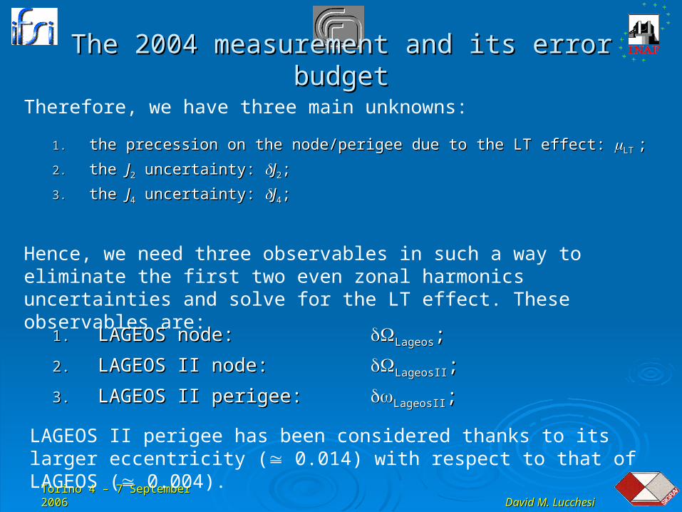
Therefore, we have three main unknowns:
1.1. the precession on the node/perigee due to the LT effect: the precession on the node/perigee due to the LT effect: LTLT ;;
2.2. the the JJ22 uncertainty: uncertainty: JJ22;;
3.3. the the JJ44 uncertainty: uncertainty: JJ44;;
Hence, we need three observables in such a way to eliminate the first two even zonal harmonics uncertainties and solve for the LT effect. These observables are:
1.1. LAGEOS node: LAGEOS node: LageosLageos;;
2.2. LAGEOS II node:LAGEOS II node: LageosIILageosII;;
3.3. LAGEOS II perigee:LAGEOS II perigee: LageosIILageosII;;
LAGEOS II perigee has been considered thanks to its larger eccentricity ( 0.014) with respect to that of LAGEOS ( 0.004).
Torino 4 – 7 September 2006Torino 4 – 7 September 2006
David M. LucchesiDavid M. Lucchesi
The 2004 measurement and its error budgetThe 2004 measurement and its error budget
yrmas
kk
kk
kk LageosIILageosIILageosLageosIILageosIILageosLT /1.60576.318.30
21
21
21
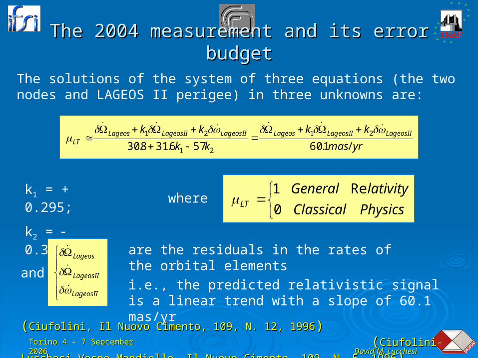
The solutions of the system of three equations (the two nodes and LAGEOS II perigee) in three unknowns are:
k1 = + 0.295;
k2 = 0.350;
PhysicsClassical
lativityGeneralLT 0
Re1where
and
LageosII
LageosII
Lageos
are the residuals in the rates of the orbital elements
((Ciufolini, Il Nuovo Cimento, 109, N. 12, 1996Ciufolini, Il Nuovo Cimento, 109, N. 12, 1996))
((Ciufolini-Lucchesi-Vespe-Mandiello, Il Nuovo Cimento, 109, N. 5, 1996Ciufolini-Lucchesi-Vespe-Mandiello, Il Nuovo Cimento, 109, N. 5, 1996))
i.e., the predicted relativistic signal is a linear trend with a slope of 60.1 mas/yr
Torino 4 – 7 September 2006Torino 4 – 7 September 2006
David M. LucchesiDavid M. Lucchesi
The 2004 measurement and its error budgetThe 2004 measurement and its error budget
yrmas
K
K
K LageosIILageosLageosIILageosLT 1.486.318.30
3
3
3
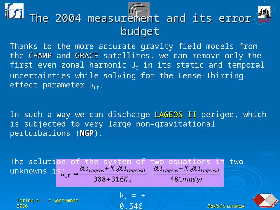
Thanks to the more accurate gravity field models from the CHAMPCHAMP and GRACEGRACE satellites, we can remove only the first even zonal harmonic J2 in its static and temporal uncertainties while solving for the Lense–Thirring effect parameter LT.
In such a way we can discharge LAGEOS IILAGEOS II perigee, which is subjected to very large non–gravitational perturbations (NGPNGP).
The solution of the system of two equations in two unknowns is:
k3 = + 0.546
Torino 4 – 7 September 2006Torino 4 – 7 September 2006
David M. LucchesiDavid M. Lucchesi
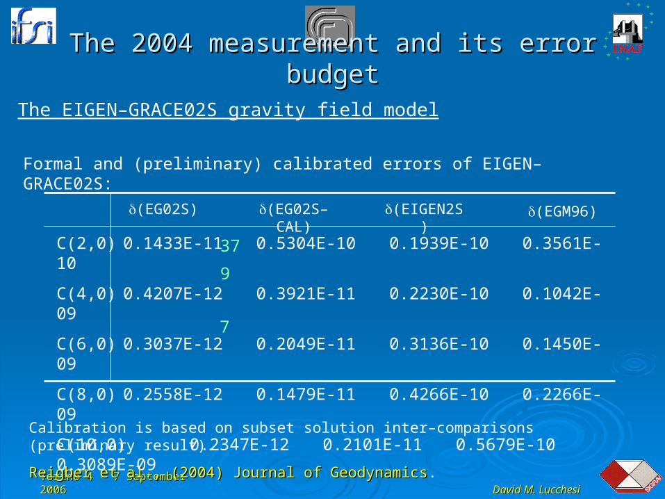
The EIGEN–GRACE02S gravity field model
Calibration is based on subset solution inter–comparisons (preliminary result).
Reigber et al., (2004)Reigber et al., (2004) Journal of Geodynamics Journal of Geodynamics.
C(2,0) 0.1433E-11 0.5304E-10 0.1939E-10 0.3561E-10
C(4,0) 0.4207E-12 0.3921E-11 0.2230E-10 0.1042E-09
C(6,0) 0.3037E-12 0.2049E-11 0.3136E-10 0.1450E-09
C(8,0) 0.2558E-12 0.1479E-11 0.4266E-10 0.2266E-09
C(10,0) 0.2347E-12 0.2101E-11 0.5679E-10 0.3089E-09
(EG02S) (EG02S–CAL) (EIGEN2S) (EGM96)
Formal and (preliminary) calibrated errors of EIGEN–GRACE02S:
37
9
7
The 2004 measurement and its error budgetThe 2004 measurement and its error budget

Torino 4 – 7 September 2006Torino 4 – 7 September 2006
David M. LucchesiDavid M. Lucchesi
The 2004 measurement and its error budgetThe 2004 measurement and its error budget
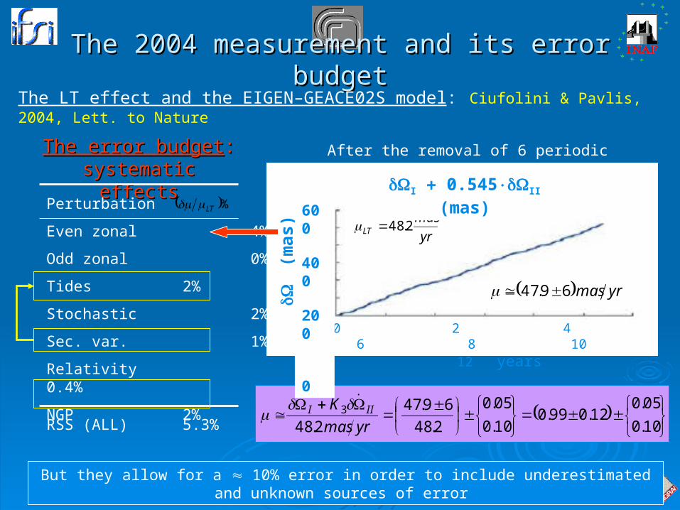
a) Observed (and combined) residuals of LAGEOS and LAGEOS II nodes (raw data);
b) As in a) after the removal of six periodic signals: 1044 days; 905 days; 281 days; 569 days and 111 days;
The best fit line through these observed residuals has a slope of about:
= (47.9 6) mas/yr
i.e., 0.99 LT
c) The theoretical Lense–Thirring effect on the node–node combination: the slope is about 48.2 mas/yr;
The LT effect and the EIGEN–GEACE02S model: Ciufolini & Pavlis, 2004, Lett. to NatureCiufolini & Pavlis, 2004, Lett. to Nature
11 years analysis of the LAGEOS’s orbit
LageosIILageos K 3
yrmasLT 2.48
Torino 4 – 7 September 2006Torino 4 – 7 September 2006
David M. LucchesiDavid M. Lucchesi
The 2004 measurement and its error budgetThe 2004 measurement and its error budget
The error budgetThe error budget: : systematic effectssystematic effects
Perturbation
Even zonal 4%
Odd zonal 0%
Tides 2%
Stochastic 2%
Sec. var. 1%
Relativity 0.4%
NGP 2%
%LT
RSS (ALL) 5.3%
10.0
05.012.099.0
10.0
05.0
2.48
69.47
2.483
yrmas
K III
But they allow for a 10% error in order to include underestimated and unknown sources of error
0 2 4 6 8 10 12 years
yr
masLT 2.48
I 0.545II (mas)
(m
as)
600
400
200
0
yrmas69.47
After the removal of 6 periodic terms
The LT effect and the EIGEN–GEACE02S model: Ciufolini & Pavlis, 2004, Lett. to Nature
Torino 4 – 7 September 2006Torino 4 – 7 September 2006
David M. LucchesiDavid M. Lucchesi
The 2004 measurement and its error budgetThe 2004 measurement and its error budget
• We are interested in reviewing such error budget because of some criticism raised in the literature to the estimate performed by Ciufolini and Pavlis.
• In particular, the secular variations of the even zonal harmonics were suggested to contribute at the level of 11% of the relativistic precession over the time span of the measurement, i.e., over 11 years.
• Moreover, also the question of possible correlations between the various sources of error and the imprinting of the Lense–Thirring effect itself in the gravity field coefficients was raised.
Torino 4 – 7 September 2006Torino 4 – 7 September 2006
David M. LucchesiDavid M. Lucchesi
Table of ContentsTable of Contents
Gravitomagnetism and Lense–Thirring effect;Gravitomagnetism and Lense–Thirring effect; The LAGEOS satellites and SLR;The LAGEOS satellites and SLR; The 2004 measurement and its error budget (EB);The 2004 measurement and its error budget (EB); The reviewed EB and the J-dot contribution;The reviewed EB and the J-dot contribution; Difficulties in improving the present measurement Difficulties in improving the present measurement
with LAGEOS satellites only;with LAGEOS satellites only; Conclusions;Conclusions;
Torino 4 – 7 September 2006Torino 4 – 7 September 2006
David M. LucchesiDavid M. Lucchesi
The reviewed EB and the J-dot contributionThe reviewed EB and the J-dot contribution
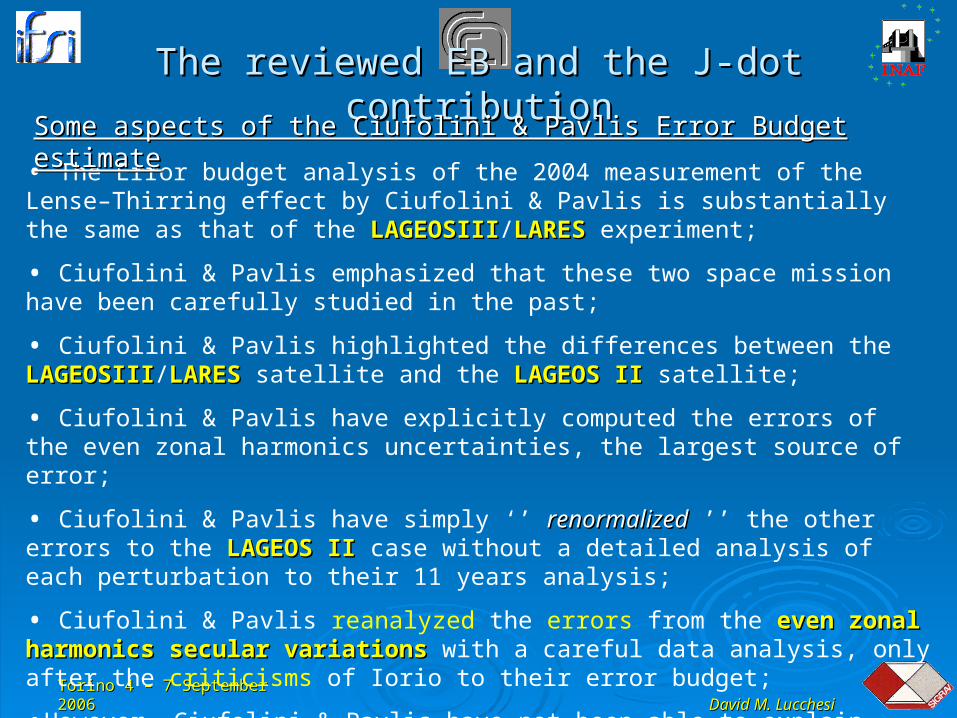
• The Error budget analysis of the 2004 measurement of the Lense–Thirring effect by Ciufolini & Pavlis is substantially the same as that of the LAGEOSIIILAGEOSIII/LARESLARES experiment;
• Ciufolini & Pavlis emphasized that these two space mission have been carefully studied in the past;
• Ciufolini & Pavlis highlighted the differences between the LAGEOSIIILAGEOSIII/LARESLARES satellite and the LAGEOS IILAGEOS II satellite;
• Ciufolini & Pavlis have explicitly computed the errors of the even zonal harmonics uncertainties, the largest source of error;
• Ciufolini & Pavlis have simply ‘’ renormalizedrenormalized ’’ the other errors to the LAGEOS IILAGEOS II case without a detailed analysis of each perturbation to their 11 years analysis;
• Ciufolini & Pavlis reanalyzed the errors from the even zonal harmonics secular even zonal harmonics secular variationsvariations with a careful data analysis, only after the criticisms of Iorio to their error budget;
•However, Ciufolini & Pavlis have not been able to explain their results from the physical point of view;
Some aspects of the Ciufolini & Pavlis Error Budget estimateSome aspects of the Ciufolini & Pavlis Error Budget estimate
Torino 4 – 7 September 2006Torino 4 – 7 September 2006
David M. LucchesiDavid M. Lucchesi
The reviewed EB and the J-dot contributionThe reviewed EB and the J-dot contribution
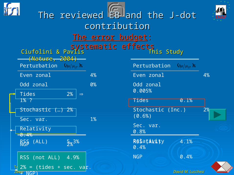
The error budgetThe error budget: systematic effects: systematic effects
Perturbation
Even zonal 4%
Odd zonal 0%
Tides 2% 1% ?
Stochastic (…) 2%
Sec. var. 1%
Relativity 0.4%
NGP 2%
%LT
RSS (ALL) 5.3%
Ciufolini & Pavlis (Nature, 2004)Ciufolini & Pavlis (Nature, 2004)
Perturbation
Even zonal 4%
Odd zonal 0.005%
Tides 0.1%
Stochastic (Inc.) 2% (0.6%)
Sec. var. 0.8%
Relativity 0.4%
NGP 0.4%
%LT
RSS (ALL) 4.1%
This StudyThis Study
RSS (not ALL) 4.9%
2% = (tides + sec. var. + NGP)
Torino 4 – 7 September 2006Torino 4 – 7 September 2006
David M. LucchesiDavid M. Lucchesi
The reviewed EB and the J-dot contributionThe reviewed EB and the J-dot contribution
The error budgetThe error budget: systematic effects: systematic effects
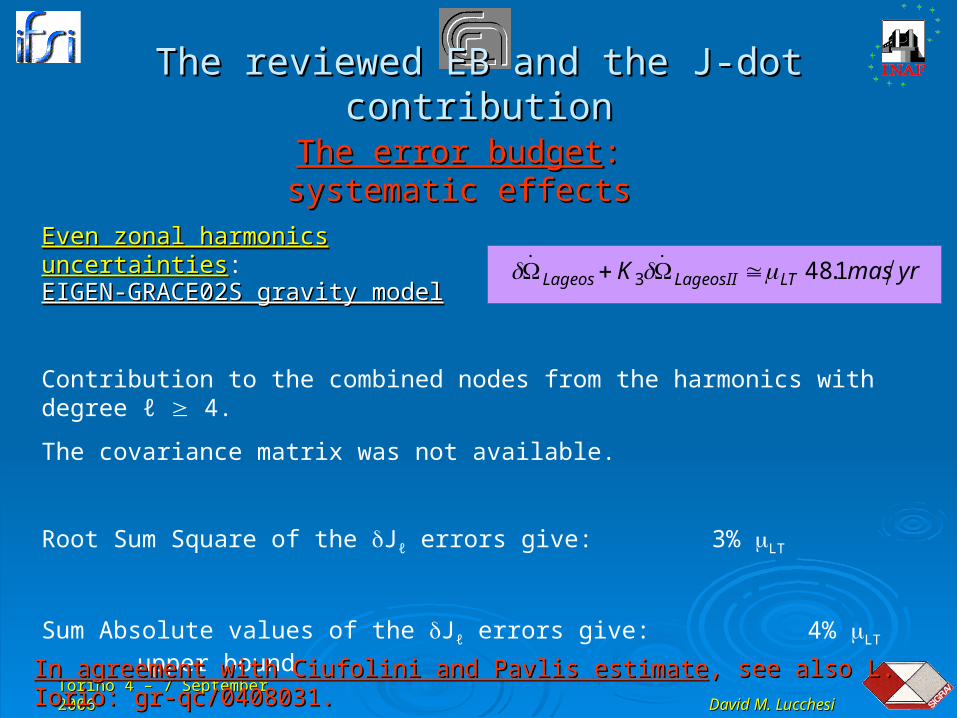
Even zonal harmonics uncertaintiesEven zonal harmonics uncertainties:
yrmasK LTLageosIILageos 1.483 EIGEN-GRACE02S gravity modelEIGEN-GRACE02S gravity model
Contribution to the combined nodes from the harmonics with degree ℓ 4.
The covariance matrix was not available.
Root Sum Square of the Jℓ errors give: 3% LT
Sum Absolute values of the Jℓ errors give: 4% LT upper bound
In agreement with Ciufolini and Pavlis estimateIn agreement with Ciufolini and Pavlis estimate, see also L. Iorio: gr-qc/0408031., see also L. Iorio: gr-qc/0408031.
Torino 4 – 7 September 2006Torino 4 – 7 September 2006
David M. LucchesiDavid M. Lucchesi
The reviewed EB and the J-dot contributionThe reviewed EB and the J-dot contribution
The error budgetThe error budget: systematic effects: systematic effects
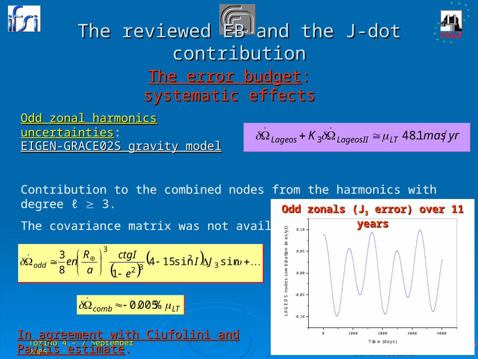
Odd zonal harmonics uncertaintiesOdd zonal harmonics uncertainties:
yrmasK LTLageosIILageos 1.483 EIGEN-GRACE02S gravity modelEIGEN-GRACE02S gravity model
Contribution to the combined nodes from the harmonics with degree ℓ 3.
The covariance matrix was not available.
sinsin15418
33
232
3
JIe
ctgI
a
Renodd
LTcomb %005.0
0 1000 2000 3000 4000
-0,10
-0,05
0,00
0,05
0,10
LAG
EO
S n
odes
com
bina
tion
(mas
/yr)
Time (days)
Odd zonals (JOdd zonals (J33 error) over 11 years error) over 11 years
In agreement with Ciufolini and Pavlis estimateIn agreement with Ciufolini and Pavlis estimate..
Torino 4 – 7 September 2006Torino 4 – 7 September 2006
David M. LucchesiDavid M. Lucchesi
0 2 4 6 8 10 12 14
-10
-5
0
5
10 LAGEOS
Nod
e sh
ift a
mpl
itude
due
to ti
des
(mas
)
Initial Phase (radians)
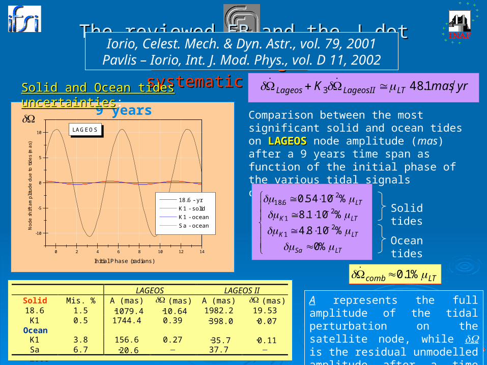
18.6 - yr K1 - solid K1 - ocean Sa - ocean
LAGEOS LAGEOS II Solid Mis. % A (mas) (mas) A (mas) (mas) 18.6 1.5 1079.4 10.64 1982.2 19.53 K1 0.5 1744.4 0.39 398.0 0.07
Ocean K1 3.8 156.6 0.27 35.7 0.11 Sa 6.7 20.6 37.7
Comparison between the most significant solid and ocean tides on LAGEOSLAGEOS node amplitude (mas) after a 9 years time span as function of the initial phase of the various tidal signals considered.
9 years
A represents the full amplitude of the tidal perturbation on the satellite node, while is the residual unmodelled amplitude after a time span of about 9 years.
LTSa
LTK
LTK
LT
%0
%108.4
%101.8
%1054.0
21
21
26.18
Solid tides
Ocean tides
The reviewed EB and the J-dot contributionThe reviewed EB and the J-dot contributionThe error budgetThe error budget: systematic effects: systematic effects
Solid and Ocean tides uncertaintiesSolid and Ocean tides uncertainties:
yrmasK LTLageosIILageos 1.483
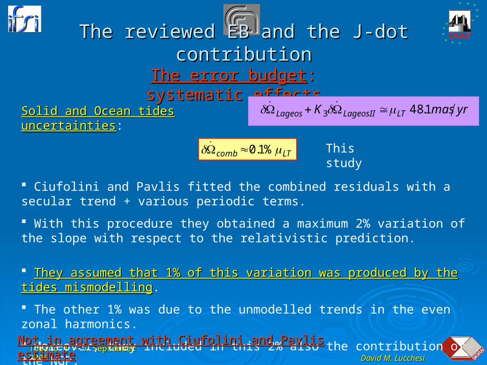
LTcomb %1.0
Iorio, Celest. Mech. & Dyn. Astr., vol. 79, 2001 Pavlis – Iorio, Int. J. Mod. Phys., vol. D 11, 2002
Torino 4 – 7 September 2006Torino 4 – 7 September 2006
David M. LucchesiDavid M. Lucchesi
The reviewed EB and the J-dot contributionThe reviewed EB and the J-dot contribution
The error budgetThe error budget: systematic effects: systematic effects
Solid and Ocean tides uncertaintiesSolid and Ocean tides uncertainties: yrmasK LTLageosIILageos 1.483
LTcomb %1.0
Ciufolini and Pavlis fitted the combined residuals with a secular trend + various periodic terms.
With this procedure they obtained a maximum 2% variation of the slope with respect to the relativistic prediction.
They assumed that 1% of this variation was produced by the tides mismodellingThey assumed that 1% of this variation was produced by the tides mismodelling.
The other 1% was due to the unmodelled trends in the even zonal harmonics.
Moreover, they included in this 2% also the contribution of the NGP.
This study
Not in agreement with Ciufolini and Pavlis estimateNot in agreement with Ciufolini and Pavlis estimate.
Torino 4 – 7 September 2006Torino 4 – 7 September 2006
David M. LucchesiDavid M. Lucchesi
The reviewed EB and the J-dot contributionThe reviewed EB and the J-dot contribution
The error budgetThe error budget: systematic effects: systematic effects
Stochastic errorsStochastic errors:
Ciufolini and Pavlis considered the following effects:
yrmasK LTLageosIILageos 1.483
seasonal variations of the Earth gravity field;
drag and observation biases;
random errors;
measurement uncertainty (random and systematic) in the inclination of LAGEOSLAGEOS satellites;
They estimated an error of about: LTstochas %2
In the present study we directly consider only the In the present study we directly consider only the measurement errors of the inclinationmeasurement errors of the inclination
Torino 4 – 7 September 2006Torino 4 – 7 September 2006
David M. LucchesiDavid M. Lucchesi
The reviewed EB and the J-dot contributionThe reviewed EB and the J-dot contribution
The error budgetThe error budget: systematic effects: systematic effects
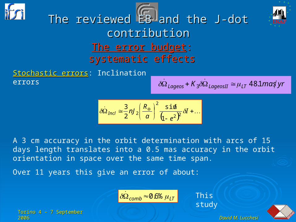
Stochastic errorsStochastic errors: Inclination errors
A 3 cm accuracy in the orbit determination with arcs of 15 days length translates into a 0.5 mas accuracy in the orbit orientation in space over the same time span.
yrmasK LTLageosIILageos 1.483
Over 11 years this give an error of about:
Ie
I
a
RnJIncl
22
2
21
sin
2
3
LTcomb %6.0 This study
Torino 4 – 7 September 2006Torino 4 – 7 September 2006
David M. LucchesiDavid M. Lucchesi
The reviewed EB and the J-dot contributionThe reviewed EB and the J-dot contribution
The error budgetThe error budget: systematic effects: systematic effects
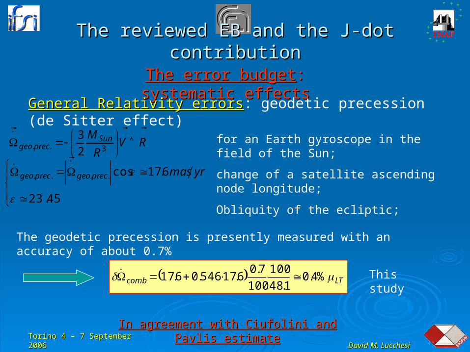
General Relativity errorsGeneral Relativity errors: geodetic precession (de Sitter effect)
RVR
M Sunprecgeo
3.. 2
3
45.23
6.17cos....
yrmasprecgeoprecgeo
for an Earth gyroscope in the field of the Sun;
change of a satellite ascending node longitude;
Obliquity of the ecliptic;
LTcomb %4.01.48
100
100
7.06.17546.06.17 This study
In agreement with Ciufolini and Pavlis estimateIn agreement with Ciufolini and Pavlis estimate
The geodetic precession is presently measured with an accuracy of about 0.7%
Torino 4 – 7 September 2006Torino 4 – 7 September 2006
David M. LucchesiDavid M. Lucchesi
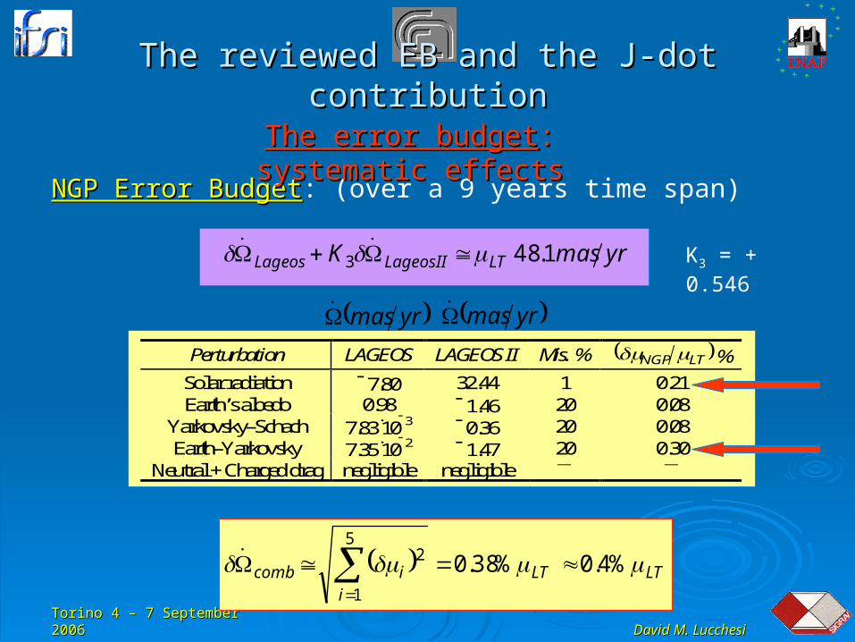
Perturbation LAGEOS LAGEOS II Mis. % LTNGP %
Solar radiation 7.80 32.44 1 0.21 Earth’s albedo 0.98 1.46 20 0.08
Yarkovsky–Schach 7.83103 0.36 20 0.08
Earth–Yarkovsky 7.35102 1.47 20 0.30
Neutral + Charged drag negligible negligible
NGP Error BudgetNGP Error Budget: (over a 9 years time span)
yrmasK LTLageosIILageos 1.483 K3 = + 0.546
yrmas yrmas
LTLTi
icomb %4.0%38.05
1
2
The reviewed EB and the J-dot contributionThe reviewed EB and the J-dot contribution
The error budgetThe error budget: systematic effects: systematic effects
Torino 4 – 7 September 2006Torino 4 – 7 September 2006
David M. LucchesiDavid M. Lucchesi
The reviewed EB and the J-dot contributionThe reviewed EB and the J-dot contribution
The error budgetThe error budget: systematic effects: systematic effects
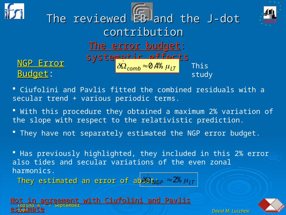
LTcomb %4.0 This study
Ciufolini and Pavlis fitted the combined residuals with a secular trend + various periodic terms.
With this procedure they obtained a maximum 2% variation of the slope with respect to the relativistic prediction.
They have not separately estimated the NGP error budget.
Has previously highlighted, they included in this 2% error also tides and secular variations of the even zonal harmonics.
Not in agreement with Ciufolini and Pavlis estimateNot in agreement with Ciufolini and Pavlis estimate.
NGP Error BudgetNGP Error Budget:
They estimated an error of about:They estimated an error of about: LTNGP %2
Torino 4 – 7 September 2006Torino 4 – 7 September 2006
David M. LucchesiDavid M. Lucchesi
The reviewed EB and the J-dot contributionThe reviewed EB and the J-dot contribution
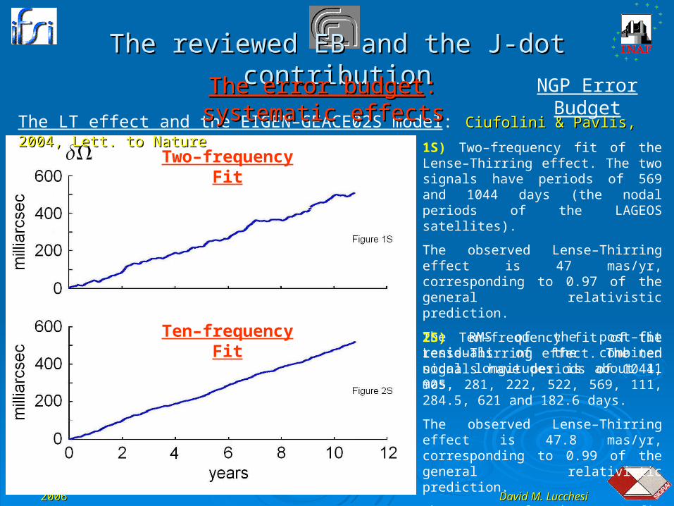
The LT effect and the EIGEN–GEACE02S model: Ciufolini & Pavlis, 2004, Lett. to NatureCiufolini & Pavlis, 2004, Lett. to Nature
1S) Two–frequency fit of the Lense–Thirring effect. The two signals have periods of 569 and 1044 days (the nodal periods of the LAGEOS satellites).
The observed Lense–Thirring effect is 47 mas/yr, corresponding to 0.97 of the general relativistic prediction.
The RMS of the post–fit residuals of the combined nodal longitudes is about 11 mas.
2S) Ten–frequency fit of the Lense–Thirring effect. The ten signals have periods of 1044, 905, 281, 222, 522, 569, 111, 284.5, 621 and 182.6 days.
The observed Lense–Thirring effect is 47.8 mas/yr, corresponding to 0.99 of the general relativistic prediction.
The RMS of the post–fit residuals is about 5.5 mas.
Two–frequency Fit
Ten–frequency Fit
The error budgetThe error budget: systematic effects: systematic effects NGP Error Budget
Torino 4 – 7 September 2006Torino 4 – 7 September 2006
David M. LucchesiDavid M. Lucchesi
The reviewed EB and the J-dot contributionThe reviewed EB and the J-dot contribution
The error budgetThe error budget: systematic effects: systematic effects
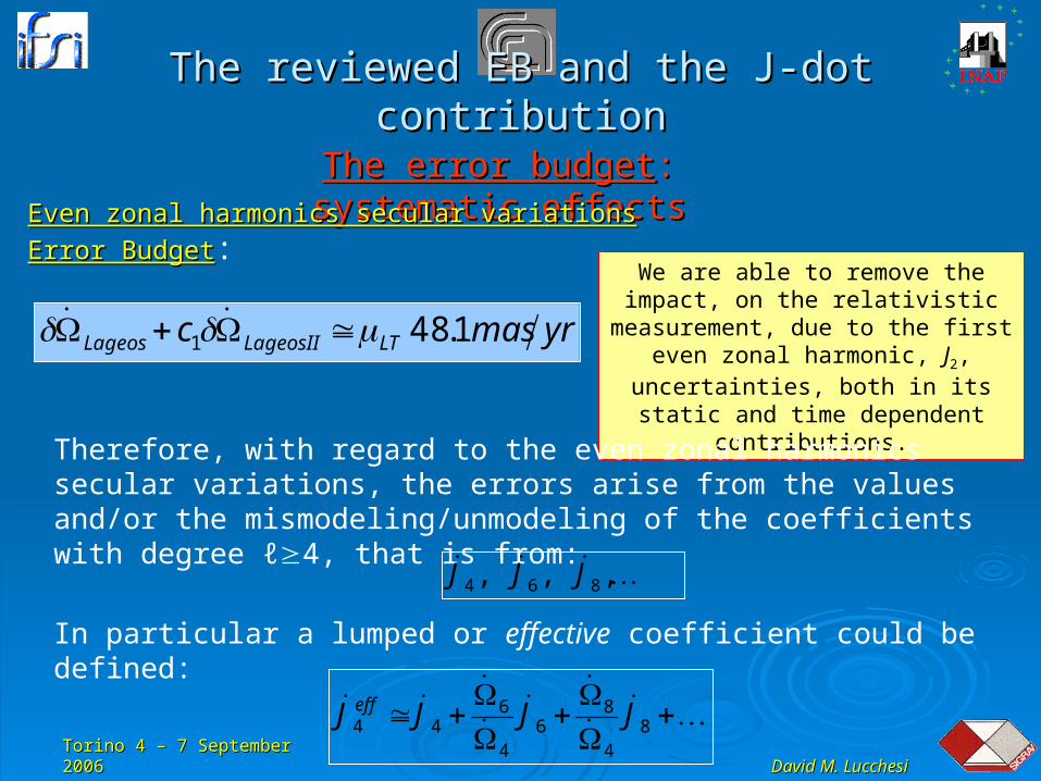
Even zonal harmonics secular variations Error BudgetEven zonal harmonics secular variations Error Budget:
We are able to remove the impact, on the relativistic measurement, due to the
first even zonal harmonic, J2, uncertainties, both in its static and time
dependent contributions.
84
86
4
644 JJJJ eff
Therefore, with regard to the even zonal harmonics secular variations, the errors arise from the values and/or the mismodeling/unmodeling of the coefficients with degree ℓ4, that is from:
,,, 864 JJJ
In particular a lumped or effective coefficient could be defined:
yrmasc LTLageosIILageos 1.481
Torino 4 – 7 September 2006Torino 4 – 7 September 2006
David M. LucchesiDavid M. Lucchesi
The reviewed EB and the J-dot contributionThe reviewed EB and the J-dot contribution
The error budgetThe error budget: systematic effects: systematic effects
Even zonal harmonics secular variations Error BudgetEven zonal harmonics secular variations Error Budget:
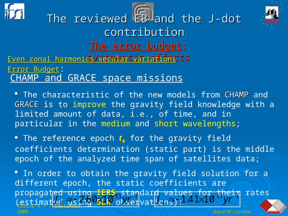
CHAMP and GRACE space missions
The characteristic of the new models from CHAMPCHAMP and GRACEGRACE is to improve the gravity field knowledge with a limited amount of data, i.e., of time, and in particular in the medium and short wavelengths;
The reference epoch tt00 for the gravity field coefficients determination (static part) is the middle epoch of the analyzed time span of satellites data;
In order to obtain the gravity field solution for a different epoch, the static coefficients are propagated using IERSIERS standard values for their rates (estimated using SLRSLR observations):
1112 1060.2 yrJ 111
4 1041.1 yrJ
Torino 4 – 7 September 2006Torino 4 – 7 September 2006
David M. LucchesiDavid M. Lucchesi
The reviewed EB and the J-dot contributionThe reviewed EB and the J-dot contribution
The error budgetThe error budget: systematic effects: systematic effects
Even zonal harmonics secular variations Error BudgetEven zonal harmonics secular variations Error Budget:
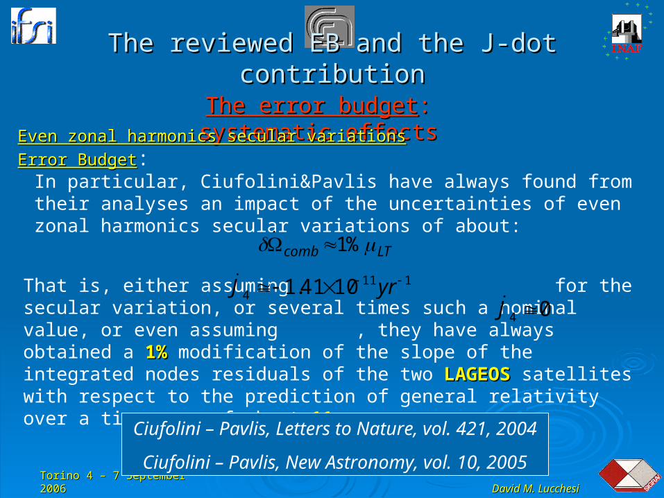
That is, either assuming for the secular variation, or several times such a nominal value, or even assuming , they have always obtained a 1%1% modification of the slope of the integrated nodes residuals of the two LAGEOSLAGEOS satellites with respect to the prediction of general relativity over a time span of about 11 yr11 yr.
In particular, Ciufolini&Pavlis have always found from their analyses an impact of the uncertainties of even zonal harmonics secular variations of about:
1114 1041.1 yrJ
04 J
Ciufolini – Pavlis, Letters to Nature, vol. 421, 2004
Ciufolini – Pavlis, New Astronomy, vol. 10, 2005
LTcomb %1
Torino 4 – 7 September 2006Torino 4 – 7 September 2006
David M. LucchesiDavid M. Lucchesi
The reviewed EB and the J-dot contributionThe reviewed EB and the J-dot contribution
The error budgetThe error budget: systematic effects: systematic effects
Even zonal harmonics secular variations Error BudgetEven zonal harmonics secular variations Error Budget:
from the nodal rate
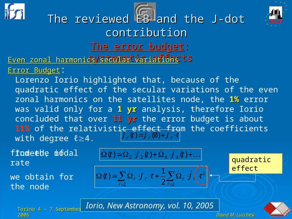
Lorenzo Iorio highlighted that, because of the quadratic effect of the secular variations of the even zonal harmonics on the satellites node, the 1%1% error was valid only for a 1 yr1 yr analysis, therefore Iorio concluded that over 11 yr11 yr the error budget is about 11% of the relativistic effect from the coefficients with degree ℓ4.
Indeed, if
Iorio, New Astronomy, vol. 10, 2005
tJJtJ )0()(
we obtain for the node
)()()( 4422 tJtJt
2
2
2 2
1)(
tJtJt
quadratic effect
Torino 4 – 7 September 2006Torino 4 – 7 September 2006
David M. LucchesiDavid M. Lucchesi
The reviewed EB and the J-dot contributionThe reviewed EB and the J-dot contribution
The error budgetThe error budget: systematic effects: systematic effects
Even zonal harmonics secular variations Error BudgetEven zonal harmonics secular variations Error Budget:
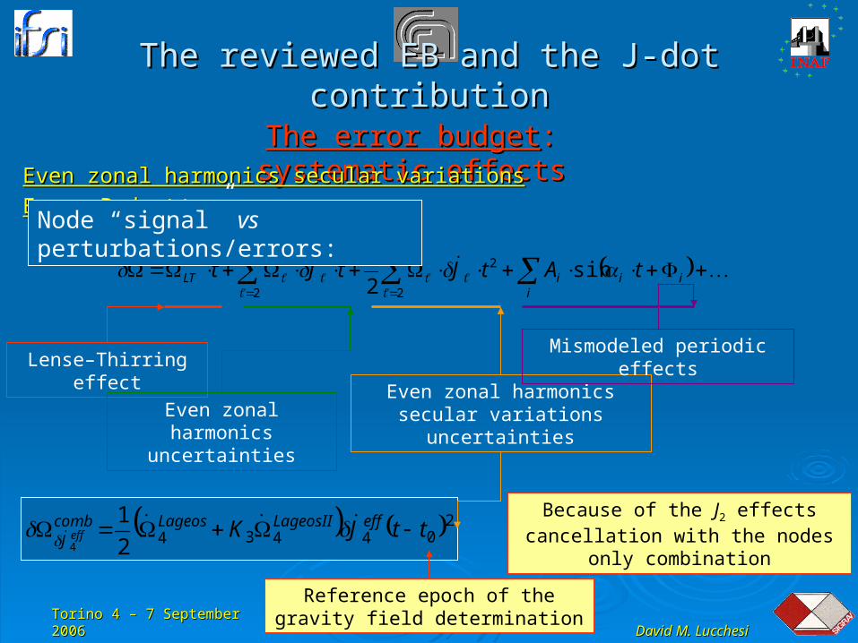
i
iiiLT tAtJtJt sin2
1
2
2
2
Lense–Thirring effect
Even zonal harmonics uncertainties
Even zonal harmonics secular variations uncertainties
Mismodeled periodic effects
Node “signal” vs perturbations/errors:
2044342
14
ttJK effLageosIILageoscombJ eff
Because of the J2 effects cancellation with the nodes only combination
Reference epoch of the gravity field determination
Torino 4 – 7 September 2006Torino 4 – 7 September 2006
David M. LucchesiDavid M. Lucchesi
The reviewed EB and the J-dot contributionThe reviewed EB and the J-dot contribution
The error budgetThe error budget: systematic effects: systematic effects
Even zonal harmonics secular variations Error BudgetEven zonal harmonics secular variations Error Budget:
0 500 1000 1500 2000 2500 3000 3500 4000
-100
0
100
200
300
400
500
Com
bine
d re
sidu
als:
I
+c1
II (m
as)
Time (days)
0 500 1000 1500 2000 2500 3000 3500 4000
-100
0
100
200
300
400
500
Com
bine
d re
sidu
als:
I
+c1
II (m
as)
Time (days)
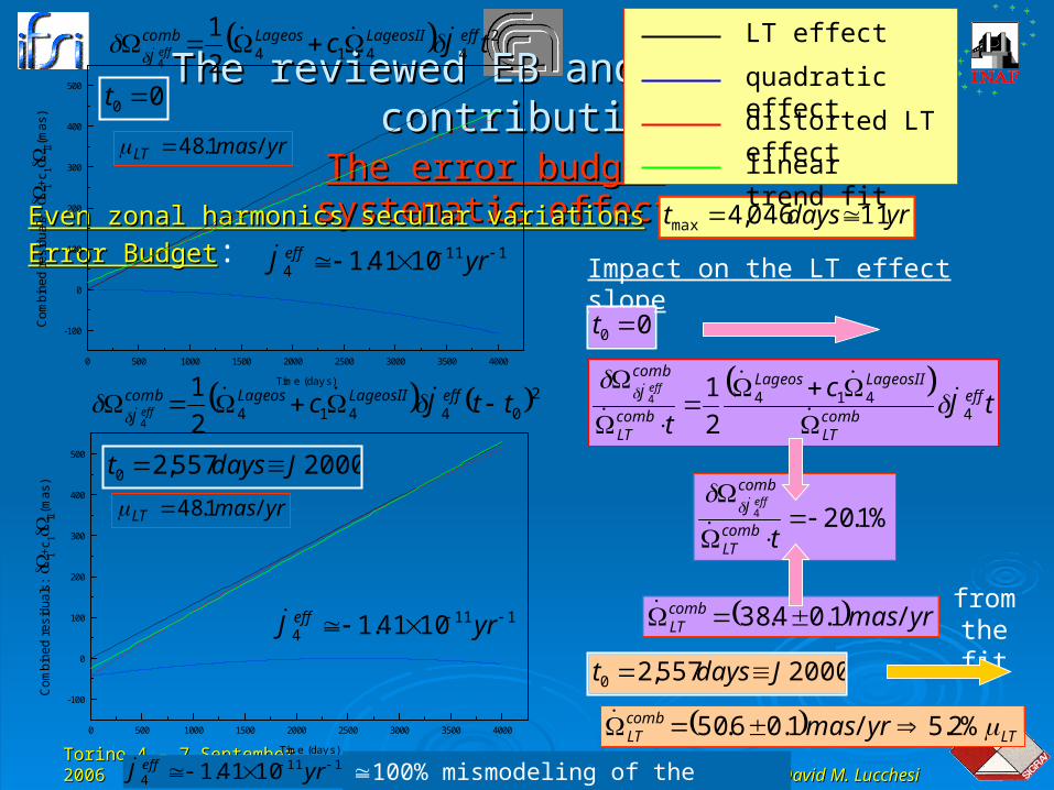
2044142
14
ttJc effLageosIILageoscomb
J eff
244142
14
tJc effLageosIILageoscomb
J eff
1114 1041.1 yrJ eff
1114 1041.1 yrJ eff
00 t
2000557,20 Jdayst
yrdayst 11046,4max
Impact on the LT effect slope
LT effect
quadratic effect
distorted LT effect
linear trend fit
tJ
c
teff
combLT
LageosIILageos
combLT
comb
J eff
4414
2
14
%1.204
tcombLT
comb
J eff
00 t
yrmascombLT /1.04.38
from the fit
2000557,20 Jdayst
LTcombLT yrmas %2.5/1.06.50
1114 1041.1 yrJ eff 100% mismodeling of the quadratic effect
yrmasLT /1.48
yrmasLT /1.48
Torino 4 – 7 September 2006Torino 4 – 7 September 2006
David M. LucchesiDavid M. Lucchesi
The reviewed EB and the J-dot contributionThe reviewed EB and the J-dot contribution
The error budgetThe error budget: systematic effects: systematic effects
Even zonal harmonics secular variations Error BudgetEven zonal harmonics secular variations Error Budget:
0 500 1000 1500 2000 2500 3000 3500 4000
-100
0
100
200
300
400
500
Com
bine
d re
sidu
als:
I
+c1
II (m
as)
Time (days)
0 500 1000 1500 2000 2500 3000 3500 4000
-100
0
100
200
300
400
500
Com
bine
d re
sidu
als:
I
+c1
II (m
as)
Time (days)
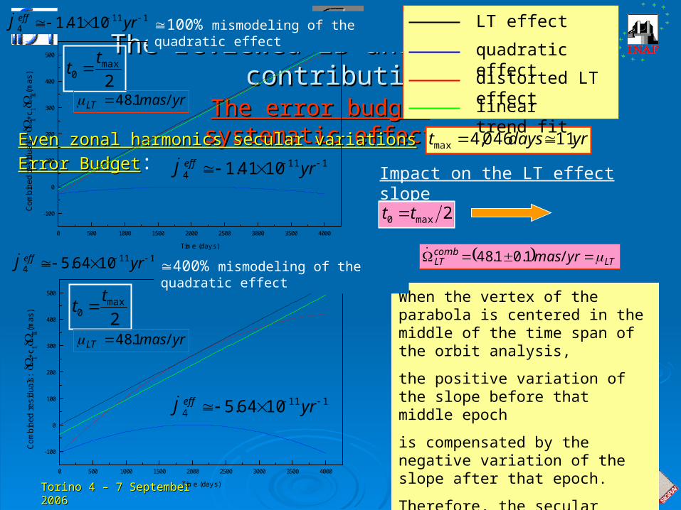
yrdayst 11046,4max
Impact on the LT effect slope
LT effect
quadratic effect
distorted LT effect
linear trend fit
2max
0
tt
2max
0
tt
1114 1041.1 yrJ eff
1114 1064.5 yrJ eff
1114 1041.1 yrJ eff 100% mismodeling of the quadratic effect
When the vertex of the parabola is centered in the middle of the time span of the orbit analysis,
the positive variation of the slope before that middle epoch
is compensated by the negative variation of the slope after that epoch.
Therefore, the secular variations have no impact on the slope of the relativistic effect.
1114 1064.5 yrJ eff 400% mismodeling of the quadratic
effect
2max0 tt
LTcombLT yrmas /1.01.48
yrmasLT /1.48
yrmasLT /1.48
Torino 4 – 7 September 2006Torino 4 – 7 September 2006
David M. LucchesiDavid M. Lucchesi
The reviewed EB and the J-dot contributionThe reviewed EB and the J-dot contribution
The error budgetThe error budget: systematic effects: systematic effects
Even zonal harmonics secular variations Error BudgetEven zonal harmonics secular variations Error Budget:
How this new approach has been How this new approach has been reachedreached
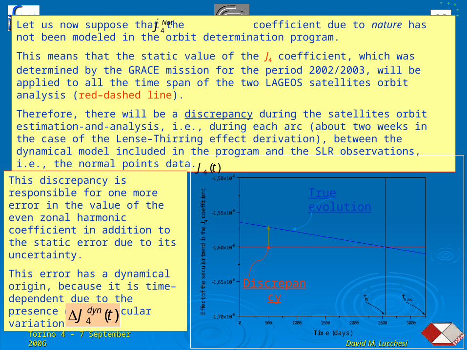
Let us now suppose that the coefficient due to nature has not been modeled in the orbit determination program.
This means that the static value of the J4 coefficient, which was determined by the GRACE mission for the period 2002/2003, will be applied to all the time span of the two LAGEOS satellites orbit analysis (red–dashed line).
Therefore, there will be a discrepancy during the satellites orbit estimation-and-analysis, i.e., during each arc (about two weeks in the case of the Lense–Thirring effect derivation), between the dynamical model included in the program and the SLR observations, i.e., the normal points data.
NatJ 4
0 500 1000 1500 2000 2500 3000-1,70x10⁻⁶
-1,65x10⁻⁶
-1,60x10⁻⁶
-1,55x10⁻⁶
-1,50x10⁻⁶
tmaxt0
Time (days)
Effe
ct o
f the
sec
ular
tren
d in
the
J 4 c
oeff
icie
nt
)(4 tJ
True evolution
Discrepancy
This discrepancy is responsible for one more error in the value of the even zonal harmonic coefficient in addition to the static error due to its uncertainty.
This error has a dynamical origin, because it is time–dependent due to the presence of the secular variation.
)(4 tJ dyn

Torino 4 – 7 September 2006Torino 4 – 7 September 2006
David M. LucchesiDavid M. Lucchesi
The reviewed EB and the J-dot contributionThe reviewed EB and the J-dot contribution
0 500 1000 1500 2000 2500 3000-1,70x10⁻⁶
-1,65x10⁻⁶
-1,60x10⁻⁶
-1,55x10⁻⁶
-1,50x10⁻⁶
tmaxt0
Time (days)
Effe
ct o
f the
sec
ular
tren
d in
the
J 4 c
oeff
icie
nt
)(4 tJ
True evolution
Discrepancy2)( 44
tJtJ Natdyn
22
)( 0max44
044max44
ttJ
tJtJ NatcombNatcombdyncomb
Over a time span t the dynamic error is given by:
and this quantity has a linear impact on the node Eq:
i
iiiLT tAtJtJt sin2
1
2
2
2
In the case of the combined nodes, the resultant error over the analyzed time span becomes:
and this error compensates exactly the impact of the parabola on the slope of the relativistic Lense–Thirring effect.
Torino 4 – 7 September 2006Torino 4 – 7 September 2006
David M. LucchesiDavid M. Lucchesi
The reviewed EB and the J-dot contributionThe reviewed EB and the J-dot contribution
The error budgetThe error budget: systematic effects: systematic effects
Even zonal harmonics secular variations Error BudgetEven zonal harmonics secular variations Error Budget:
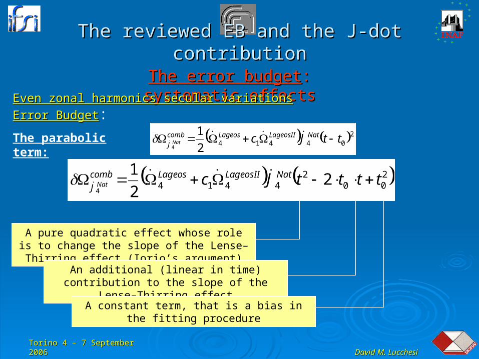
2044142
14
ttJc NatLageosIILageoscomb
J Nat The parabolic term:
200
24414 2
2
14
ttttJc NatLageosIILageoscomb
J Nat
A pure quadratic effect whose role is to change the slope of the Lense–Thirring effect (Iorio’s argument)
An additional (linear in time) contribution to the slope of the Lense–Thirring effect
A constant term, that is a bias in the fitting procedure
Torino 4 – 7 September 2006Torino 4 – 7 September 2006
David M. LucchesiDavid M. Lucchesi
The reviewed EB and the J-dot contributionThe reviewed EB and the J-dot contribution
The error budgetThe error budget: systematic effects: systematic effects
Even zonal harmonics secular variations Error BudgetEven zonal harmonics secular variations Error Budget:
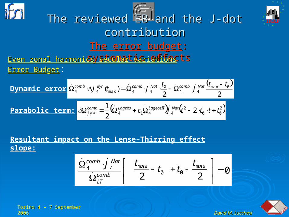
044
combLT
Natcomb J
0
max
2t
t
2max
0
tt
200
24414 2
2
14
ttttJc NatLageosIILageoscomb
J Nat
22
)( 0max44
044max44
ttJ
tJtJ NatcombNatcombdyncomb
Parabolic term:
Dynamic error:
Resultant impact on the Lense–Thirring effect slope:

Torino 4 – 7 September 2006Torino 4 – 7 September 2006
David M. LucchesiDavid M. Lucchesi
The reviewed EB and the J-dot contributionThe reviewed EB and the J-dot contribution
The error budgetThe error budget: systematic effects: systematic effects
Even zonal harmonics secular variations Error BudgetEven zonal harmonics secular variations Error Budget:
200
24414 2
2
14
ttttJc NatLageosIILageoscomb
J Nat
22
)( 0max44
044max44
ttJ
tJtJ NatcombNatcombdyncomb
Parabolic term:
Dynamic error:
We stress that the role of the dynamic error is not to cancel the parabola, but to cancel its impact on the Lense–Thirring effect slope, that is, its effect is to shift the symmetry axis of the parabola, i.e., the epoch t0, to the value tmax/2.
tmy
ctbtay 2 ctmbtay 2
The resultant effect is to change the position of the symmetry axis, the vertex and the
focus of the parabola, but not its concavity.
2
21
2
22
21
2max
44
max00
44
t
J
ttt
Ja
mbt
Natcomb
Natcomb
Symmetry axis:
Lucchesi, Int. Journ. of Modern Phys. D, vol. 14, No. 12, 2005
Torino 4 – 7 September 2006Torino 4 – 7 September 2006
David M. LucchesiDavid M. Lucchesi
The reviewed EB and the J-dot contributionThe reviewed EB and the J-dot contribution
The error budgetThe error budget: systematic effects: systematic effects
Even zonal harmonics secular variations Error BudgetEven zonal harmonics secular variations Error Budget:
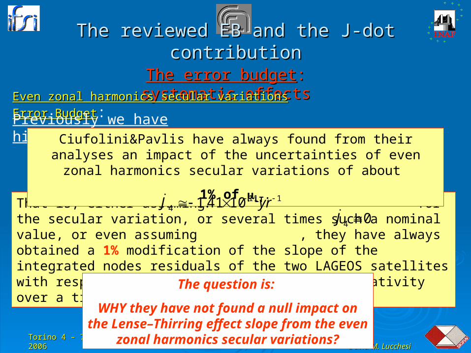
Previously we have highlighted that:
That is, either assuming for the secular variation, or several times such a nominal value, or even assuming , they have always obtained a 1% modification of the slope of the integrated nodes residuals of the two LAGEOS satellites with respect to the prediction of general relativity over a time span of about 11 yr.
Ciufolini&Pavlis have always found from their analyses an impact of the uncertainties of even zonal harmonics secular variations of about
1% of LT.111
4 1041.1 yrJ04 J
The question is:
WHY they have not found a null impact on the Lense–Thirring effect slope from the
even zonal harmonics secular variations?
Torino 4 – 7 September 2006Torino 4 – 7 September 2006
David M. LucchesiDavid M. Lucchesi
The reviewed EB and the J-dot contributionThe reviewed EB and the J-dot contribution
The error budgetThe error budget: systematic effects: systematic effects
Even zonal harmonics secular variations Error BudgetEven zonal harmonics secular variations Error Budget:
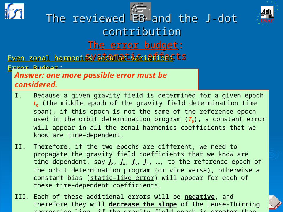
Answer: one more possible error must be considered.
I. Because a given gravity field is determined for a given epoch t0 (the middle epoch of the gravity field determination time span), if this epoch is not the same of the reference epoch used in the orbit determination program (T0), a constant error will appear in all the zonal harmonics coefficients that we know are time–dependent.
II. Therefore, if the two epochs are different, we need to propagate the gravity field coefficients that we know are time–dependent, say J2, J4, J6, J8, …, to the reference epoch of the orbit determination program (or vice versa), otherwise a constant bias (static–like error) will appear for each of these time–dependent coefficients.
III. Each of these additional errors will be negative, and therefore they will decrease the slope of the Lense–Thirring regression line, if the gravity field epoch is greater than T0, and positive (hence increasing the slope) if the gravity field epoch is smaller than T0.
IV. This error will change the b coefficient of the parabola and will shift away its symmetry axis from the time tmax/2.
Torino 4 – 7 September 2006Torino 4 – 7 September 2006
David M. LucchesiDavid M. Lucchesi
The reviewed EB and the J-dot contributionThe reviewed EB and the J-dot contribution
The error budgetThe error budget: systematic effects: systematic effects
Even zonal harmonics secular variations Error BudgetEven zonal harmonics secular variations Error Budget:
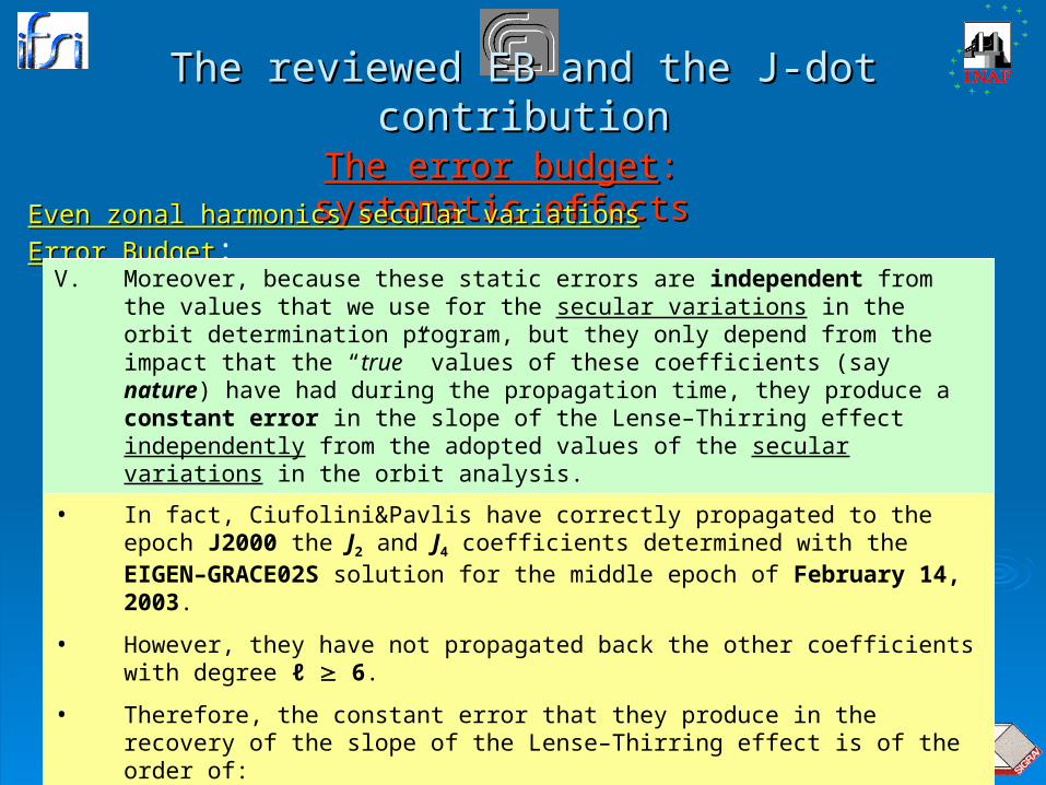
V. Moreover, because these static errors are independent from the values that we use for the secular variations in the orbit determination program, but they only depend from the impact that the “true” values of these coefficients (say nature) have had during the propagation time, they produce a constant error in the slope of the Lense–Thirring effect independently from the adopted values of the secular variations in the orbit analysis.
VI. This is very important and represents the key to explain the 1% error in the recovery of the slope of the Lense–Thirring effect in all the simulations performed by Ciufolini&Pavlis.
0066 TtJ effcombcombLT
• In fact, Ciufolini&Pavlis have correctly propagated to the epoch J2000 the J2 and J4 coefficients determined with the EIGEN–GRACE02S solution for the middle epoch of February 14, 2003.
• However, they have not propagated back the other coefficients with degree ℓ 6.
• Therefore, the constant error that they produce in the recovery of the slope of the Lense–Thirring effect is of the order of:

Torino 4 – 7 September 2006Torino 4 – 7 September 2006
David M. LucchesiDavid M. Lucchesi
The reviewed EB and the J-dot contributionThe reviewed EB and the J-dot contribution
The error budgetThe error budget: systematic effects: systematic effects
Even zonal harmonics secular variations Error BudgetEven zonal harmonics secular variations Error Budget: Therefore, we obtain:
combLT
NateffcombeffcombcombLT TtJJTtJ %8.0004440066
where:
1114 105.1 yrJ eff
1114 1041.1 yrJ
comes from their fit of the quadratic effect
comes from IERS standard
yrTt 1.300 comes from the discrepancy of the two reference epochs
The result is very close to the 1% error claimed by Ciufolini&Pavlis.
The discrepancy is probably due to the effects of the periodic perturbations that are also present in the integrated node residuals obtained with the EIGEN–GRACE02S gravity field model.
Lucchesi, Int. Journ. of Modern Phys. D, vol. 14, No. 12, 2005
Torino 4 – 7 September 2006Torino 4 – 7 September 2006
David M. LucchesiDavid M. Lucchesi
Table of ContentsTable of Contents
Gravitomagnetism and Lense–Thirring effect;Gravitomagnetism and Lense–Thirring effect; The LAGEOS satellites and SLR;The LAGEOS satellites and SLR; The 2004 measurement and its error budget (EB);The 2004 measurement and its error budget (EB); The reviewed EB and the J-dot contribution;The reviewed EB and the J-dot contribution; Difficulties in improving the present measurement Difficulties in improving the present measurement
with LAGEOS satellites only;with LAGEOS satellites only; Conclusions;Conclusions;
Torino 4 – 7 September 2006Torino 4 – 7 September 2006
David M. LucchesiDavid M. Lucchesi
Difficulties in improving the present measurement with Difficulties in improving the present measurement with LAGEOS satellites onlyLAGEOS satellites only
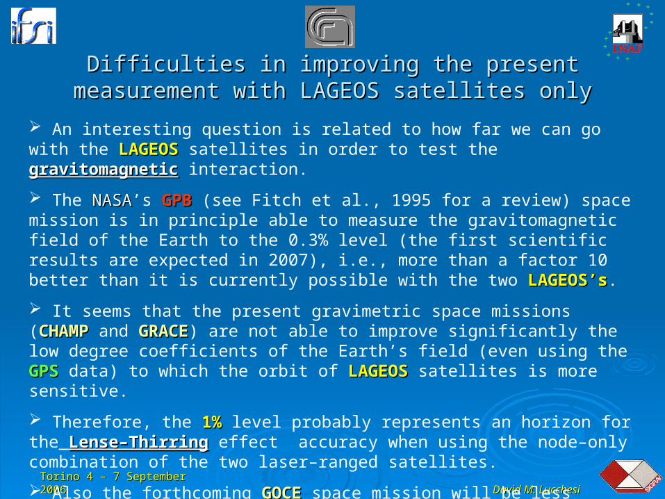
An interesting question is related to how far we can go with the LAGEOSLAGEOS satellites in order to test the gravitomagneticgravitomagnetic interaction.
The NASA NASA’s GPBGPB (see Fitch et al., 1995 for a review) space mission is in principle able to measure the gravitomagnetic field of the Earth to the 0.3% level (the first scientific results are expected in 2007), i.e., more than a factor 10 better than it is currently possible with the two LAGEOS’sLAGEOS’s.
It seems that the present gravimetric space missions (CHAMPCHAMP and GRACEGRACE) are not able to improve significantly the low degree coefficients of the Earth’s field (even using the GPSGPS data) to which the orbit of LAGEOSLAGEOS satellites is more sensitive.
Therefore, the 1%1% level probably represents an horizon for the Lense–ThirringLense–Thirring effect accuracy when using the node–only combination of the two laser–ranged satellites.
Also the forthcoming GOCEGOCE space mission will be less sensitive to the low degree components of the Earth’s field and not so great improvements are expected.
Torino 4 – 7 September 2006Torino 4 – 7 September 2006
David M. LucchesiDavid M. Lucchesi
Difficulties in improving the present measurement with Difficulties in improving the present measurement with LAGEOS satellites onlyLAGEOS satellites only
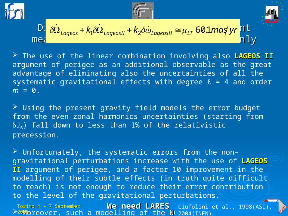
The use of the linear combination involving also LAGEOS IILAGEOS II argument of perigee as an additional observable as the great advantage of eliminating also the uncertainties of all the systematic gravitational effects with degree ℓ = 4 and order m = 0.
Using the present gravity field models the error budget from the even zonal harmonics uncertainties (starting from J6) fall down to less than 1% of the relativistic precession.
Unfortunately, the systematic errors from the non–gravitational perturbations increase with the use of LAGEOS IILAGEOS II argument of perigee, and a factor 10 improvement in the modelling of their subtle effects (in truth quite difficult to reach) is not enough to reduce their error contribution to the level of the gravitational perturbations.
Moreover, such a modelling of the NGPNGP requires an improvement also in the range accuracy of the SLRSLR technique. Again, a not easy task.
We need LARES !We need LARES ! Ciufolini et al., 1998(ASI), 2004(INFN)
yrmaskk LTLageosIILageosIILageos 1.6021
Torino 4 – 7 September 2006Torino 4 – 7 September 2006
David M. LucchesiDavid M. Lucchesi
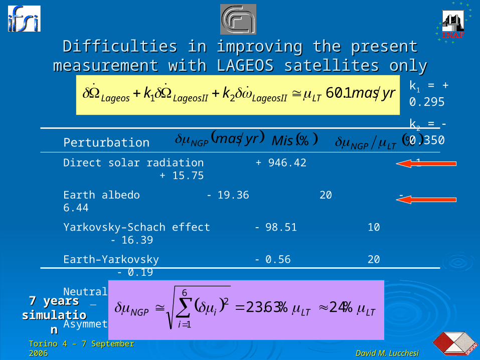
Difficulties in improving the present measurement with Difficulties in improving the present measurement with LAGEOS satellites onlyLAGEOS satellites only
Direct solar radiation + 946.42 1 + 15.75
Earth albedo 19.36 20 6.44
Yarkovsky–Schach effect 98.51 10 16.39
Earth–Yarkovsky 0.56 20 0.19
Neutral + Charged particle drag negligible negligible
Asymmetric reflectivity
Perturbation yrmasNGP %LTNGP %.Mis
yrmaskk LTLageosIILageosIILageos 1.6021
LTLTi
iNGP %24%63.236
1
2
k1 = + 0.295
k2 = 0.350
7 years 7 years simulationsimulation
Torino 4 – 7 September 2006Torino 4 – 7 September 2006
David M. LucchesiDavid M. Lucchesi
Difficulties in improving the present measurement with Difficulties in improving the present measurement with LAGEOS satellites onlyLAGEOS satellites only
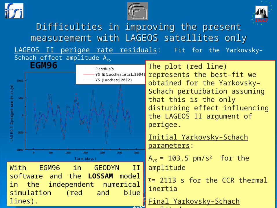
LAGEOS II perigee rate residuals: Fit for the Yarkovsky–Schach effect amplitude AYS
Lucchesi, Ciufolini, Andrés, Pavlis, Peron, Noomen and Currie, Plan. Space Science, 52, 2004
0 500 1000 1500 2000 2500 3000-10000
-5000
0
5000
10000
Residuals YS fit (Lucchesi et al., 2004) YS (Lucchesi, 2002)
LAG
EO
S II
per
igee
rate
(mas
/yr)
Time (days)
EGM96 The plot (red line) represents the best–fit we obtained for the Yarkovsky–Schach perturbation assuming that this is the only disturbing effect influencing the LAGEOS II argument of perigee.
Initial Yarkovsky–Schach parameters:
AYS = 103.5 pm/s2 for the amplitude
= 2113 s for the CCR thermal inertia
Final Yarkovsky–Schach amplitude:
AYS = 193.2 pm/s2
i.e., about 1.9 times the pre–fit value.
With EGM96 in GEODYN II software and the LOSSAM model in the independent numerical simulation (red and blue lines).
Torino 4 – 7 September 2006Torino 4 – 7 September 2006
David M. LucchesiDavid M. Lucchesi
Difficulties in improving the present measurement with Difficulties in improving the present measurement with LAGEOS satellites onlyLAGEOS satellites only
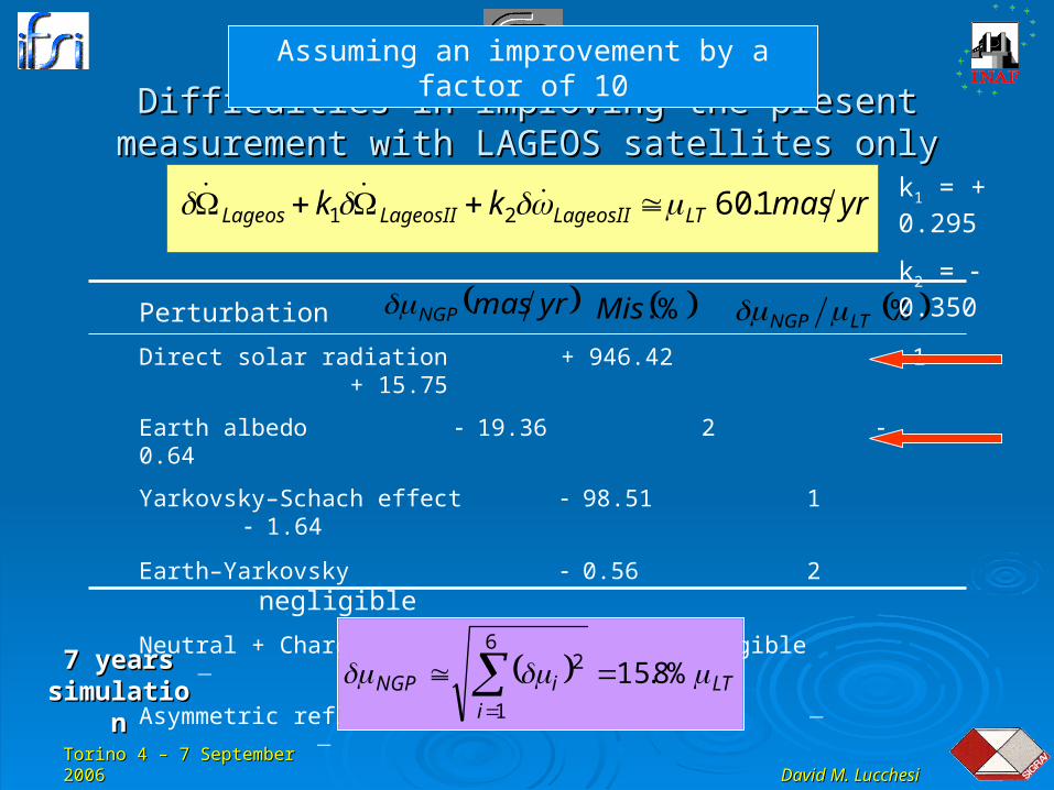
Direct solar radiation + 946.42 1 + 15.75
Earth albedo 19.36 2 0.64
Yarkovsky–Schach effect 98.51 1 1.64
Earth–Yarkovsky 0.56 2 negligible
Neutral + Charged particle drag negligible negligible
Asymmetric reflectivity
Perturbation yrmasNGP %LTNGP %.Mis
yrmaskk LTLageosIILageosIILageos 1.6021
LTi
iNGP %8.156
1
2
k1 = + 0.295
k2 = 0.350
7 years 7 years simulationsimulation
Assuming an improvement by a factor of 10

Torino 4 – 7 September 2006Torino 4 – 7 September 2006
David M. LucchesiDavid M. Lucchesi
Difficulties in improving the present measurement with Difficulties in improving the present measurement with LAGEOS satellites onlyLAGEOS satellites only
The Largest (and Best Modelled) NGPNGP on LAGEOSLAGEOS and LAGEOS IILAGEOS II orbit is due to direct solar radiation pressure (SRPSRP):
sD
D
mc
ACa
Sun
SunSunRSun ˆ
2
3.6·109 m/s2
CR represents the satellite radiation coefficient, about 1.12 for LAGEOS IILAGEOS II;
A/m represents the area–to–mass ratio of the satellites, about 7104 m2/kg;
Sun represents the solar irradiance at 1 AU, about 1380 W/m2;
c represents the speed of light, about 3108 m/s;
DSun represents the average Earth–Sun distance, i.e., 1 AU;
ŝ represents the Earth–Sun unit vector;
Where:
211104 smaSun
Error in SRP SRP :
yrmaskk LTLageosIILageosIILageos 1.6021
Torino 4 – 7 September 2006Torino 4 – 7 September 2006
David M. LucchesiDavid M. Lucchesi
Difficulties in improving the present measurement with Difficulties in improving the present measurement with LAGEOS satellites onlyLAGEOS satellites only
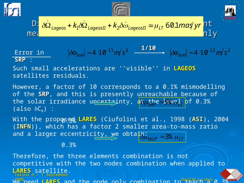
211104 smaSun
Error in SRP SRP :
1/101/10 212104 smaSun
Such small accelerations are ‘’visible’’ in LAGEOSLAGEOS satellites residuals.
However, a factor of 10 corresponds to a 0.1% mismodelling of the SRPSRP, and this is presently unreachable because of the solar irradiance uncertainty, at the level of 0.3% (also CR) :
0.3% LTSRP %5
yrmaskk LTLageosIILageosIILageos 1.6021
With the proposed LARESLARES (Ciufolini et al., 1998 (ASIASI), 2004 (INFNINFN)), which has a factor 2 smaller area-to-mass ratio and a larger eccentricity, we obtain:
0.3%
Therefore, the three elements combination is not competitive with the two nodes combination when applied to LARESLARES satellite.
We need LARESLARES and the node only combination to reach a 0.3% measurement of the Lense–ThirringLense–Thirring effect (Lucchesi&Rubincam, 2004Lucchesi&Rubincam, 2004).
LTNGP %3

Torino 4 – 7 September 2006Torino 4 – 7 September 2006
David M. LucchesiDavid M. Lucchesi
Table of ContentsTable of Contents
Gravitomagnetism and Lense–Thirring effect;Gravitomagnetism and Lense–Thirring effect; The LAGEOS satellites and SLR;The LAGEOS satellites and SLR; The 2004 measurement and its error budget (EB);The 2004 measurement and its error budget (EB); The reviewed EB and the J-dot contribution;The reviewed EB and the J-dot contribution; Difficulties in improving the present measurement Difficulties in improving the present measurement
with LAGEOS satellites only;with LAGEOS satellites only; Conclusions;Conclusions;
Torino 4 – 7 September 2006Torino 4 – 7 September 2006
David M. LucchesiDavid M. Lucchesi
ConclusionsConclusions
1. From the results of the present analysis the overall error budget of the 2004 measurement of the Lense–ThirringLense–Thirring effect seems reliable, about 5% at 1–sigma level;
2. In particular, the impact of the even zonal harmonics secular trends is around 1% of the relativistic prediction;
3. However, the error budget of the 2004 measurement is not characterized by a clear separation of the individual contributions to the resultant error budget, in particular in the periodic effects;
4. We have tried to better quantify such contributions to the error budget, in particular:
i) we have explained from the physical point of view the 1% error due to the i) we have explained from the physical point of view the 1% error due to the secular trends of the even zonal harmonics;secular trends of the even zonal harmonics;
ii) we have estimated the contribution of the main tidal signals as well as of the ii) we have estimated the contribution of the main tidal signals as well as of the NGP;NGP;
Torino 4 – 7 September 2006Torino 4 – 7 September 2006
David M. LucchesiDavid M. Lucchesi
ConclusionsConclusions
5. We have underlined the difficulties in improving the present results using LAGEOSLAGEOS satellites only: the LARESLARES satellites is necessary in addition to the two LAGEOSLAGEOS;
6.6. LARESLARES will be competitive with GPBGPB goal: a 0.3% measurement;
7.7. LARESLARES will be very useful not only for fundamental physicsfundamental physics in space but also for space geodesy and geodynamicsgeodesy and geodynamics;
8. Waiting to LARESLARES mission (?) and GPBGPB results (2007), it will be very useful a new measurement of the Lense–ThirringLense–Thirring effect with the two LAGEOSLAGEOS satellites together with the measurement of the first even zonal harmonics coefficients, those at which the two satellites orbit are most sensitive to, in such a way to obtain a reliable error budget at a few % level;
finis