Issuer Quality and Corporate Bond Returns

Robin Greenwood and Samuel G. Hanson

Harvard University

February 2013 (First draft: September 2010)

Abstract

We show that the credit quality of corporate debt issuers deteriorates during credit booms, and that this deterioration forecasts low excess returns to corporate bondholders. The key insight is that changes in the pricing of credit risk disproportionately affect the financing costs faced by low quality firms, so the debt issuance of low quality firms is particularly useful for forecasting bond returns. We show that a significant decline in issuer quality is a more reliable signal of credit market overheating than rapid aggregate credit growth. We use these findings to investigate the forces driving time-variation in expected corporate bond returns.

                                                             For helpful suggestions, we are grateful to Malcolm Baker, Effi Benmelech, Dan Bergstresser, John Campbell, Sergey Chernenko, Lauren Cohen, Ian Dew-Becker, Martin Fridson, Victoria Ivashina, Chris Malloy, Andrew Metrick, Jun Pan, Erik Stafford, Luis Viceira, Jeff Wurgler, seminar participants at the 2012 AEA Annual Meetings, Columbia GSB, Dartmouth Tuck, Federal Reserve Bank of New York, Federal Reserve Board of Governors, Harvard Business School, MIT Sloan, NYU Stern, Ohio State Fisher, University of Chicago Booth, University of Pennsylvania Wharton, Washington University Olin, Yale SOM, and especially David Scharfstein, Andrei Shleifer, Jeremy Stein, and Adi Sunderam. We thank Annette Larson and Morningstar for data on bond returns and Mara Eyllon and William Lacy for research assistance. The Division of Research at the Harvard Business School provided funding.

 

1  

In most modern accounts of the credit cycle, fluctuations in the quantity of credit are driven

by time-varying financing frictions, due to changes in borrowers’ net worth or in bank capital

(Bernanke and Gertler (1989); Holmstrom and Tirole (1997); Kiyotaki and Moore (1997); and

Kashyap, Stein, and Wilcox (1993)). Notably absent from these accounts is the possibility that time-

varying investor beliefs or tastes play a role in determining the quantity and allocation of credit. This

absence is surprising given abundant evidence of historical periods – such as the 1980s junk bond era

or the credit boom of 2004-2007 – when credit markets appear to have become overheated,

potentially reflecting heightened investor risk appetites or over-optimism.1 During these periods,

investors granted credit at low promised yields to borrowers of poor quality, and experienced low

returns when these borrowers later defaulted and credit spreads widened. In this paper we draw on

more than 80 years of historical data to show that this pattern – deteriorating issuer quality followed

by low investor returns – should be understood as a recurring feature of the credit cycle.

Our approach is to link patterns of corporate debt financing to time-series variation in the

pricing of credit risk. The key insight is that broad changes in the pricing of credit risk

disproportionately affect the financing costs faced by low credit quality firms. To the extent that

firms issue more debt when credit is “cheap,” the debt issuance of low credit quality firms may then

be a particularly useful barometer of financing conditions. Specifically, time-variation in debt issuer

quality may be useful for forecasting excess corporate bond returns: risky corporate bonds should

underperform default-free government bonds following periods when corporate debt issuers are of

particularly poor credit quality. To be clear, we are not claiming that issuer quality causes low future

bond returns; issuer quality may forecast corporate bond returns because firms respond to time-

variation in the cost of capital.

To test this hypothesis, we form time-series measures of debt issuer quality. Our primary

                                                            1 See Kaplan and Stein (1993) and Grant (1992) on the 1980s LBO and junk bond boom, Coval, Jurek, and Stafford (2009) on the 2000s structured finance boom, Axelson, Jenkinson, Stromberg, and Weisbach (2010), Ivashina and Sun (2010) and Shivdasani and Wang (2009) on the 2000s leveraged loan and LBO boom, and Demyanyk and Van Hemert (2011) on the deterioration of mortgage loans prior to the subprime crisis.

 

2  

measure compares the average credit quality of firms with high debt issuance – proxied using each

firm’s expected default frequency – to the credit quality of firms with low debt issuance. A second

measure is constructed from credit ratings: each year from 1926 to 2008, we compute the fraction of

corporate bond issuance that is rated speculative grade. Building on Hickman (1958), Atkinson

(1967), and Bernanke, Gertler, and Gilchrist (1996), we show that variation in issuer quality is a

central feature of the credit cycle: when aggregate credit increases, the average quality of issuers

deteriorates.

We use these measures of issuer quality to forecast the excess returns on corporate bonds.

Following periods when issuer quality is poor, corporate bonds significantly underperform Treasury

bonds of similar maturities. The degree of return predictability is large in both economic and

statistical terms. The predictability is most striking for high yield bonds – with univariate R2 statistics

up to 30% at a 3-year horizon – but similar results obtain for investment grade bonds, albeit with

diminished magnitude. Issuer quality has incremental forecasting power for corporate bond returns

over and above other macros variables that researchers have used to forecast corporate bond returns,

including credit spreads and the term spread. Our results also obtain when we control for the Fama

and French (1993) stock market factors (contemporaneous with the bond returns)—suggesting that

we are capturing alpha in our forecasting regressions. Furthermore, the quality of debt issuance is a

better forecaster of excess corporate bond returns than the aggregate quantity of debt issuance.

In summary, our results demonstrate a high degree of predictability in corporate bond returns

that is linked to the composition of corporate debt financing. Flipping this relationship around,

expected bond returns appear to be an important driver of the mix of firms that are borrowing at any

point in time, so the results may be of independent interest from a corporate finance standpoint.  For

instance, our results are related to Erel, Julio, Kim, and Weisbach (2011) who document that the

capital raised by high yield firms is pro-cyclical. The forecasting results imply significant time-

variation in the real cost of debt financing for firms: a one-standard deviation deterioration in issuer

 

3  

quality is associated with a reduction in the cost of credit for high-yield firms of roughly 1.66

percentage points per annum.

We then use these findings to explore the forces that drive time-series variation in expected

corporate bond excess returns. We consider three potential sources of return predictability: (1)

countercyclical variation in the rationally determined price of risk as would arise in consumption-

based asset pricing models; (2) time-variation in effective risk tolerance due to financial

intermediary-related frictions; and (3) time-varying mispricing due to investor biases in evaluating

credit risk over the cycle. In attempting to discriminate between these sources, we recognize that it is

impossible to fully rule out one explanation or another. Furthermore, there is little reason to believe

that just one channel is operational.

We first consider whether the results are consistent with consumption-based models in which

markets are integrated and the rationally determined price of risk varies in a countercyclical fashion.

For instance, investors’ risk aversion may vary due to habit formation as in Campbell and Cochrane

(1999). According to explanations of this type, investors are not systematically surprised when the

bonds of low quality firms who often receive funding during booms later underperform.

Several of our main findings are consistent with consumption-based asset pricing models.

Specifically, issuer quality has a clear business cycle component. Furthermore, when included as

controls in our return forecasting regressions, macroeconomic variables slightly attenuate the effects

of issuer quality. However, several of our findings are more difficult to square with consumption-

based models. For instance, we forecast statistically significant negative excess returns in a number

of sample years. Because credit assets typically underperform Treasuries during bad economic times,

consumption-based models would always predict positive expected excess returns. Furthermore, our

issuer quality measures are disconnected from traditional forecasters of the equity premium, and do

not forecast excess stock returns, cutting against the idea that issuer quality simply proxies for a

rationally time-varying price of risk in fully integrated stock and bond markets.

 

4  

Another source of variation in expected returns could stem from changes in intermediary risk

tolerance. For example, a number of authors have argued that fluctuations in intermediary equity

capital may drive changes in risk premia. We examine a number of proxies for intermediary balance

sheet strength, including lagged intermediary capital ratios and balance sheet growth. Several of these

measures are correlated with issuer quality in the expected direction (e.g., issuer quality tends to be

poor when insurers, which are large holders of corporate bonds, have high equity capital ratios).

However, the forecasting power of issuer quality is not impacted by the addition of intermediary-

related controls.

A slightly different intermediary-based explanation is suggested by Rajan (2005), who argues

that agency problems may encourage some institutions to “reach for yield,” buying riskier assets with

high promised yields when riskless interest rates are low. Consistent with this idea, we show that

issuer quality declines when yields on Treasury bonds are low or have recently fallen. On the other

hand, interest rate controls do little to affect the forecasting power of issuer quality in our return

forecasting regressions.

A third source of variation in expected returns could stem from biased investor beliefs.

Specifically, investors may make biased assessments of default probabilities, leading to time-varying

mispricing of credit. One natural bias might stem from over-extrapolation of past default rates or

bond returns. For example, following a string of years in which few firms default, investors may

underestimate future default probabilities, leading them to bid up the prices of risky corporate bonds.

As a result, investors are surprised by periods of elevated corporate defaults, resulting in sharp

declines in corporate bond prices.

Explanations that appeal investor over-extrapolation allow for negative expected excess

returns, consistent with our findings.2 And, while it is difficult to measure investors’ beliefs directly,

                                                            2 Of course, investors themselves would always expect positive excess returns, even if they have a tendency to over-extrapolate past outcomes. However, the best econometric forecast of excess returns in such a world could be significantly negative on occasion.

 

5  

the extrapolation story predicts that issuer quality should decline following periods of low defaults or

high credit returns. This pattern emerges quite strongly in the data, suggesting that the recent

experience of credit market investors may play a role in shaping investors’ expectations or tastes.

In summary, we cannot fully pin down the forces that drive variation in expected returns.

While consumption-based explanations are surely an important part of the overall story, several

pieces of evidence suggest that they may not be the full story. Specifically, the evidence hints that the

second and third channels – intermediary risk tolerance and mistaken investor beliefs – might play

some role. If we adopt this interpretation, then erosion in issuer quality may be a useful signal of

credit market overheating.

Our findings build on three strands of research. First, there is prior work in finance linking

time-varying financing patterns to expected returns (e.g., Baker and Wurgler (2000)). Related to this,

a recent line of enquiry uses government debt growth to forecast financial crises (Reinhart and

Rogoff (2008)). Second, a large literature in macroeconomics, starting with Bernanke and Gertler

(1989) attempts to understand fluctuations in the quantity of credit as a driver of the business cycle.

Third, researchers in both macroeconomics and finance have used credit spreads and other interest

rates to forecast changes in real activity (Fama (1981), Thoma and Gray (1998), Gilchrist and

Zakrajšek (2011)).

I. Empirical Design

Here we develop a reduced-form model to motivate the empirical design. In the model, debt

issuance responds to changes in the pricing of credit. The model explains why debt issuer quality may

be useful for forecasting excess credit returns. The model also pinpoints the circumstances under

which quality may be more useful than aggregate quantities for forecasting excess credit returns, and

under what circumstances quality may contain information about expected returns beyond what is

revealed by credit spreads.

A. A reduced-form model of credit spreads and debt issuance

 

6  

Assume that credit spreads (the difference between corporate bond yields and risk-free yields

of the same maturity) are equal to expected credit losses plus expected excess returns. At this point

we can be agnostic about what drives variation in expected returns: it might be a rationally time-

varying credit risk premium, time-varying mispricing, or both. As a simple reduced form, we write

the credit spread st for firms of type θ as

,tt ts  

(1)

whereθ,t is the time-varying probability of default, δt denotes the time-varying expected return on

credit assets, and βθ is the exposure of type θ firms to the market-wide pricing credit risk. Thus, the

expected excess return on bonds of type θ is

, 1[ ] .t ttE rx  

(2)

For simplicity, we assume that θt does not directly affect expected excess returns. Since default

probabilities θt vary over time, equations (1) and (2) capture the idea that spreads mean different

things at different times: spreads can be low because default probabilities are low or because

expected excess returns are low.

For simplicity, suppose firms are either low default risk L or high default risk H, with

Lt < Ht for all t. Our central assumption is that L < H. This means that the bonds of high default

risk firms are more heavily exposed to market-wide changes in the pricing of credit risk.

Firms of type θ choose their debt issuance dt (or leverage) by trading off the benefits of

issuing additional cheap debt against the costs of deviating from their target capital structure, as in

Stein (1996). Target capital structure has two independent components: a part t that is common to all

firms and a part t that is specific to firms of type θ. A variety of factors unrelated to expected

returns may cause target leverage to fluctuate, such as changes in investment opportunities. We

assume that firms choose their issuance to solve

 

7  

2

2

( ) ( / 2) ( ( ))

( / 2)( ( ))

max

max ,

t

t

t t t t t t

t t t t t

d

d

s d d

d d

 

(3)

where reflects the cost of deviating from target leverage. The optimal choice of dθt is given by

* ( / ) ,t t t td  

(4)

so firms borrow more when the expected returns on credit assets are low. A neo-classical

interpretation of equation (4) appeals to standard Q-theory logic: the optimal scale of corporate

investment, and hence debt issuance, rises when rationally required returns decline. A more

behavioral interpretation of (4) might emphasize corporate market-timing behavior.3 However, our

empirical design does not hinge on the specific interpretation one adopts.

The logic of our identification strategy can be seen immediately from equation (4). Debt

issuance is driven by changes in expected returns and by changes in target leverage. Since L H ,

fluctuations in expected returns t have a larger impact on the issuance of high default risk firms than

on the issuance of low default risk firms. Changes in target leverage are not informative about

expected returns and have a common component that is shared by all firms. Thus, it is useful to

examine the difference in debt issuance between high- and low-default risk firms.

Now, suppose that half of the firms are low default risk and the other half are high default

risk, then equation (4) implies that the total quantity of debt issuance is

* * (2 ) (( ) / ) .Ht Lt t Ht Lt H L td d  

(5)

A proxy for the issuer quality mix is the difference in debt issuance between high and low default risk

firms

                                                            3 The idea that firms can back out the component of credit spreads that is due to any time-varying mispricing may seem objectionable: it seems implausible that firms could have an informational advantage over sophisticated investors in forecasting broad changes in spreads. However, as emphasized by Greenwood, Hanson, and Stein (2010), firms may have an institutional advantage in exploiting aggregate mispricing even if they have no informational advantage. Sophisticated investors are often subject to limits of arbitrage which may be particularly relevant in the case of market-wide mispricing. By contrast, operating firms can exploit this kind of mispricing by adjusting their capital structures without the fear of performance-based withdrawals.

 

8  

* * ( ) (( ) / ) .Ht Lt Ht Lt H L td d  

(6)

By looking at the quality of issuance, we remove the impact of the common factor t which affects

the issuance of all firms. Thus, the quality mix helps isolate the information that issuance contains

about expected returns.

B. Forecasting returns using issuance quantity and quality

Under these assumptions, both quantity ( * *Ht Ltd d )  and quality  ( * *

Ht Ltd d ) will negatively

forecast excess returns in a univariate regression. In a bivariate forecasting regression that includes

both quantity and quality, the coefficients on both variables will be negative so long as 2 0 .

However, quality becomes more informative than quantity as 2 

grows large (the Internet Appendix

contains the relevant calculations.4) Intuitively, examining the quality mix should be particularly

informative if aggregate debt issuance has an important common time-series component that is

unrelated to future returns. For example, if aggregate debt issuance fluctuates significantly due to

shocks to aggregate investment opportunities, then the quality mix of issuance may be a better

predictor of returns than the total quantity of issuance. The model also suggests that the results will

be strongest when forecasting the returns of low-grade bonds which have the greatest exposure to

market-wide changes in the pricing of credit.

C. Forecasting returns using spreads and issuance quality

Credit spreads positively forecast excess returns on corporate bonds. Should issuer quality

have incremental forecasting power for returns beyond spreads? In a multivariate forecasting

regression of excess returns on credit spreads and issuer quality, the coefficient on spreads is positive

and the coefficient on * *Ht Ltd d is negative. This is because both spreads and issuer quality are

affected by factors other than expected returns. For instance, as the time-series volatility of default

                                                            4 An Internet Appendix, which includes all supplementary unreported results, is posted on the authors’ websites.

 

9  

probabilities (i.e., fundamentals) grows large, spreads become less informative about δt.5

D. Measuring issuer quality empirically

How should we measure issuer quality in the data? A first approach which follows directly

from equation (6) is to classify firms as either high or low default risks and then compare the debt

issuance of these two groups, i.e., * *Ht Ltd d . A related idea is to compute the share of debt issuance

accounted for by high default risk firms, i.e., * * */ ( )Ht Ht Ltd d d . It may also be useful to construct

measures which reflect the continuous nature of firm default risk. Thus, a third measure compares the

default risk of high debt issuers with that of low debt issuers each period

* *[ | ] [ | ],t t i it t i itISS E High d E Low d  

(7)

where we now allow quality βi and debt issuance vary continuously across firms. This construction

parallels the equity issuance-based “characteristic spreads” used in Greenwood and Hanson (2012). It

is straightforward to show that all three measures are decreasing in expected returns δt. While ISSt is

the measure we emphasize in the majority of the paper, we show that our findings are not sensitive to

the specific method we use to measure issuer quality.

II. Measuring Debt Issuer Quality

A. Compustat-based measures of issuer quality: 1962-2008

Following the above discussion, we compare the credit quality of firms issuing large amounts

of debt to that of firms issuing little debt or who are retiring debt. Specifically, in each year t, we

compute

,it it

it it

EDFt

it iti High d i Low dHigh d Low d

t t

ISSEDF EDF

N N

 

(8)

                                                            5 To see the intuition, consider the related exercise of forecasting stock returns using equity issuance and the dividend yield. Suppose a Gordon growth model holds, so D/P reflects expected returns and dividend growth – i.e., D/P = R – G. If issuance responds mechanically to D/P, it will have no incremental forecasting power. If, however, issuance responds differently to changes in R than changes in G, it may contain additional information beyond D/P.

 

10  

where EDF is an estimate of the firm’s default probability, 1/it it itd D A denotes debt issuance,

and N denotes the number of firms. Debt issuance is the change in assets minus the change in book

equity from Compustat, scaled by lagged assets. ISSEDF compares the average default probability of

high net debt issuers (net debt issuance in the top NYSE quintile) with the default probability of low

net debt issuers (net debt issuance in the bottom NYSE quintile). Thus, ISSEDF takes on high values

when debt issuers are of relatively poor credit quality.

EDF is the Merton (1974) expected default frequency, computed following Bharath and

Shumway (2008).6 A simple way to think of EDF is that it is a statistical equivalent of a credit rating,

albeit one that we can compute reliably for a larger sample of firms starting in 1963.7 Highly levered

firms with high asset volatility and low expected returns have the highest EDFs. Firms with high

EDFs also tend to be small and young, do not pay dividends, have high leverage, and have low

interest coverage. Naturally, these firms also have high estimated default probabilities based on other

forecasters, such as the Shumway (2001) bankruptcy hazard rate. Debt issues, EDF, and several

alternate measures of firm credit quality are summarized in Panel A of Table 1, with the details of

their construction given in the Internet Appendix. EDF is close to zero for the median firm, while the

mean EDF is 6%.

When substituting a firm’s EDF into equation (8), we use NYSE deciles rather than the raw

values. Using deciles minimizes the influence of outlier firms and avoids the possibility of picking up

compositional shifts in the set of listed firms or secular trends.8 It also makes the units easy to

                                                            6 For firm i in year t, Φ ln / 0.5 / where Ei,t is the market value of equity, Fi,t is the face value of debt (computed as short-term debt plus one-half long-term debt), , is the asset drift (estimated using the prior 12-month stock return), is the asset volatility (estimated as / /

0.05 0.25 where is the annualized volatility of monthly stock returns over the prior 12 months), and Φ ∙ is the standard normal CDF. 7 From 1985-2008, the correlation between EDF decile and S&P credit ratings is 0.54 for firms with a valid rating. 8 For example, if we wanted to see whether issuance was concentrated among large firms, it would make little sense to compute the average size of high issuers as the cross-sectional dispersion of size has increased over time. A limitation of using deciles is that we throw out information about changes in the cross-sectional dispersion of EDFit.

 

11  

interpret: 1EDFtISS  means that firms with high net debt issuance had EDFs that were on average

one decile higher than firms with low net debt issuance. However, as shown below, we obtain

somewhat stronger results if we compute ISSEDF using raw EDFs as opposed to EDF deciles.

We plot ISSEDF in Figure 1 and provide summary statistics for the time series in Table 1.

Table 2 lists the entire time series. ISSEDF was high (i.e., high debt issuers were of relatively poor

quality) in the mid-to-late 1960s, 1973, 1978, the mid-to-late 1980s, 1997-1998, and again in 2005-

2007. ISSEDF drops sharply in 1970-1971, 1975-1976, the early 1990s, 2001-2002, and finally in

2008.

Figure 1 also shows the relationship between ISSEDF and the business cycle. The shaded bars

denote NBER recessions. ISSEDF tends to be low in recessions and high in expansions. However, this

relation is not exact and the lead-lag relationship between the business cycle and ISSEDF varies over

time. For instance, ISSEDF falls during many recessions, but rises during the 1982 recession as the

1980s high yield boom was getting underway. The series also tends to peak before recessions, but

occasionally peaks after the economy is already in recession. We can remove the influence of the

business cycle by regressing ISSEDF on the output gap (Hodrick-Prescott (1997) filtered log real GDP)

and saving the residuals. This orthogonalized series, shown as a dashed line in Panel B, still captures

the same peaks and troughs of the original series, consistent with the idea that the credit cycle is

somewhat distinct from the business cycle.

Our time series of issuer quality corresponds closely to historical accounts of credit booms

and busts. For example, Grant (1992) describes the credit boom of the late 1960s, when our ISSEDF

series reaches its sample peak. This period saw booming corporate bond issuance and the rise of the

short-term commercial paper market, which grew from $10 billion in 1966 to over $40 billion by

early 1970. The boom came to an abrupt end following the Penn Central commercial paper default of

June 1970. Officials at the Federal Reserve Bank of New York noted the “deterioration in the quality

of outstanding paper” in the run-up to Penn Central. These events are reflected in the sharp drop in

 

12  

ISSEDF between 1968-1969 and 1970-1971.

The decline of issuer quality during the 1980s junk bond boom has been noted by a number of

authors (Grant (1992) and Kaplan and Stein (1993)). Klarman (1991) notes that financier Michael

Milken marketed new issue junk bonds on the assumption that their default rates would be similar to

those of recent high yield issues. However, default rates had been low due to strong economic growth

in an environment of declining interest rates. Klarman argues that the denominator in the default rate

calculation soared during the issuance boom, leading investors to underestimate the likelihood of

future defaults (Asquith, Mullins, and Wolff (1989)).

The robust credit markets of the mid-to-late 1990s and 2004-2007 are by now familiar.

However, ISSEDF is unlikely to capture the full extent of the 2004-2007 boom, because it is based on

corporate credit, whereas much of the credit growth and deterioration in borrower quality during this

period was in residential mortgages and structured products (see e.g., Demyanyk and Hemert (2011)).

While we do not expect ISSEDF to capture the full scale of this activity, the basic arc of the boom is

apparent in Figure 1.

Panel B of Table 1 also summarizes alternate time-series measures of issuer quality,

constructed similarly to ISSEDF. We follow the same procedure as in equation (8), but use different

firm characteristics to proxy for credit quality. For example, ISSIntcov is the difference between the

average interest coverage (decile) of high and low debt issuers. In each case, we order characteristics

so that high values of the ISS variable indicate years in which lower credit quality firms are issuing

debt. These measures of quality are all highly correlated over time.

B. The high yield share: 1926-2008

A second quality measure can be formed using the credit ratings assigned to new corporate

bond issues. We define the high yield share as the share of nonfinancial corporate bond issuance in

each year with a high yield rating from Moody’s

 

13  

,t

itHighYield

it itHighYield InvGrade

HYSB

B B

 (9)

where Bi,t denotes the principal value of bond i issued in year t.9 In our forecasting regressions, we

take the log of the raw share so that our regression coefficients can be interpreted as the change in

returns following a one percent change in HYS. 10 We use the Mergent Fixed Income Security

Database (FISD) to construct HYS from 1983-2008. We extend the series from 1926-1965 using data

from NBER studies by Hickman (1960) and Atkinson (1967) who report aggregate issuance by credit

rating based on a compilation of bond issues from Moody’s Bond Surveys. Aggregate issues by

credit rating are not available from 1966-1982, so we hand-collect information on bond offerings

from weekly editions of these books.11

Figure 2 plots HYS alongside ISSEDF for comparison, and Table 2 lists the HYS values. Similar

to ISSEDF, HYS takes on high values when issuer quality is poor. The data show a small high yield

debt boom in the late 1950s and early 1960s, and a more substantial boom in the late 1960s.

Corporate bond issuers were of particularly low quality in the late 1980s, in 1997 and 1998, and again

in 2004 and 2005. There is a clear regime shift between the first and second halves of the sample: the

level and volatility of HYS are much higher starting in the early 1980s. The correlation between HYS

and ISSEDF is 0.47 prior to 1982, and 0.58 after 1982.

                                                            9 High yield bonds are those rated Ba1 or lower by Moody's or BB+ or lower by SS&P. For simplicity, we use the S&P nomenclature (e.g., AAA, AA, A, BBB, BB, B, and C) throughout, even when working with Moody's data. 10 We use log(HYS) because it provides a good fit, but qualitatively similar results obtain if we forecast returns using HYS. To compute log(HYS), we need to address the fact that HYS = 0 in 1974. To do so, we set HYS equal to 0.0024 for 1974 before applying the log transformation (0.0024 is the second lowest value of HYS observed in sample). However, our treatment of this single observation does not play an important role in driving our results. 11 FISD is the current incarnation of the Moody’s Bond Survey, so we are essentially using the same primary source throughout. We start using FISD in 1983 because FISD only contains bonds that mature in 1990 or later. So long as speculative and investment grades issues have similar maturity distributions, this truncation should impart no bias to HYS. We exclude financials, asset-backed securities, sovereigns, and exchange offers to preserve comparability with Hickman (1960) and Atkinson (1967). The amount of bond offerings by Moody’s rating from 1926-1943 is from Table V2 of Hickman (1960) and data from 1944-1965 is from Table B-1 of Atkinson (1967). Following Atkinson and Hickman, we include convertible issues from 1966-1982. Prior to the surge in high yield issuance in the 1980s, many speculative grade issues contained conversion features.

 

14  

The advantage of HYS is its simplicity. However, there are several reasons to prefer ISSEDF.

First, ISSEDF reflects a broader measure of debt issues, including both loan and bond market

financing.12 This means that unlike HYS, ISSEDF is not be impacted by secular shifts in the relative

sizes of the markets for low-grade bonds and low-grade loans. Since the sizes of these markets have

fluctuated over time – the most prominent example being the rapid growth of the high yield bond

market in the early 1980s – this is a major strength of ISSEDF. Indeed, the level of HYS is considerably

lower prior to the early 1980s.13 Second, if loan and bond markets are partially integrated components

of the broader corporate credit market, measures based on total debt issuance (loans plus bonds) may

be more informative about future bond returns than measures based solely on bond issuance.

Specifically, if firms willingly substitute between loans and bonds, isolated shocks to bank loan

supply would induce a positive relationship between bond issuance and expected excess bond returns.

However, the relationship between total debt issuance and expected excess bond returns would

remain negative, even in the presence isolated loan supply shocks.14 Third, ISSEDF holds constant the

definition of firm quality. HYS, in contrast, relies on the assumption that the meaning of credit ratings

has remained constant. However, Blume, Lim, and MacKinlay (1998) and Baghai, Servaes, and

Tamayo (2010) argue that the agencies have become more conservative in assigning ratings since the

late 1970s. Fourth, ISSEDF is based on net rather than gross debt issuance, thus better capturing

changes in the financial position of low quality firms.

                                                            12  Empirically, ISSEDF appears to partially reflect changes in bank lending standards: changes in ISSEDF are -0.51 correlated with the Federal Reserve’s Senior Loan Officer Opinion Survey of changes in the stricture of bank lending standards from 1967-1983 (see Lown and Morgan (2006)) and 1990-2008. 13 We can compute bonds outstanding as a share of total loans and bonds for non-financial corporations from Table 102 of the Flow of Funds. This “bond share” fell steadily from 52% in 1962 to 39% in 1984 and then gradually rose again to 61% by 2003. This trend reversed from 2004-2008 as the bond share again fell to 56%, reflecting the rapid growth of the leveraged loan market. 14 To see why, suppose that lending standards are relaxed, while bond investment standards remain unchanged. Since corporations substitute between loans and bonds (see e.g., Becker and Ivashina (2010)), banks’ willingness to grant cheap credit would raise loan issuance, lower bond issuance, and lower expected bond excess returns. However, total debt issuance would rise. In summary, assuming partial substitutability between bonds and loans, total debt issuance is likely to be better reflection of broad credit supply, which in turn drives expected excess bond returns.

 

15  

Figure 2 illustrates a final limitation of HYS as a measure of issuer quality: it can be unduly

volatile in years in which total issuance (the denominator in equation (9)) is particularly low. This is

most problematic in 1933 – the historical low point for total issuance, representing a near collapse of

the corporate bond market. Because investment grade issuance fell even more dramatically than high

yield issuance in 1933, HYS spikes to its sample maximum at the nadir of the Great Depression.

While we use the full time-series of HYS in the analysis that follows, we note that removing this

single outlier significantly strengthens our forecasting results.

C. Returns and other data

Our remaining time series are summarized in Panel D of Table 1. Short-term government

bond yields ( GSty ) and the term spread ( G G

Lt Sty y ) are from Ibbotson. The credit spread ( BBB GLt Lty y ) is

the difference between the log yield of the Moody’s BBB corporate index and the log long-term

government bond yield from Ibbotson. Business cycle controls include real industrial production

growth from the Federal Reserve, real aggregate consumption growth from the BEA National Income

and Product Accounts, and a dummy variable indicating whether the year is classified as a recession

by the NBER. As an alternate business cycle control, we use Hodrick-Prescott (1997) filtered log real

GDP as a measure of the output gap. We also use the consumption wealth ratio (cay) from Lettau and

Ludvigson (2001) and the eight principal components that Ludvigson and Ng (2010) extract from 132

macroeconomic and financial time series.

Returns on high yield bonds are from Morningstar/Ibbotson from 1927-1982 and from

Barclays Capital (formerly Lehman Brothers) starting in 1983. We construct high yield excess returns

by subtracting the log return on intermediate Treasuries from Ibbotson: 1 1 1.HY HY G

t t trx r r

Intermediate Treasuries (with a maturity of approximately 5 years) are the appropriate benchmark for

 

16  

high yield bonds since the average duration on the Barclay’s high yield index is just under 5 years.15

Excess returns on BBB-rated corporate bonds (1 1 1

BBB BBB Gt t trx r r ) and AAA-rated bonds (

1 1 1AAA AAA Gt t trx r r ) are calculated in a similar fashion using Morningstar/Ibbotson data from 1927-

1989 and Barclays data beginning in 1990. We compute 2- and 3- year cumulative log excess returns

by summing 1-year log excess returns.

III. Issuer quality and excess corporate bond returns

A. Univariate forecasting regressions

Figure 3 shows the main result. We plot ISSEDF against cumulative high yield excess returns

over the following 2 years. Returns are plotted in reverse scale, so the negative correlation appears

positive visually. The correlation between the two series is -0.51. Simply put, periods of poor issuer

quality are followed by low excess returns on corporate bonds.

Table 3 shows forecasting regressions of cumulative excess returns on quality measures

,HYtt k t krx a b X u

(10)

where k denotes a forecast horizon of 1-, 2-, or 3-years and X is either ISSEDF or log(HYS). Moving

from left to right, we present forecasting regressions for ISSEDF for 1962-2008 and the 1983-2008

subsample, and HYS for 1926-2008 and the 1983-2008 subsample. We isolate the 1983-2008 period

which corresponds to the modern high yield bond market. Moving from top to bottom, the three

panels show separate regressions for the excess returns on high yield, BBB-rated, and AAA-rated

corporate bonds. Here and in subsequent tables, t-statistics for k-year regressions are based on

Newey-West (1987) standard errors, allowing for serial correlation up to k lags.

The top-left regression in Panel A shows that ISSEDF has an R2 of 12% for high yield excess                                                             15 Ibbotson bond return data are also used by Keim and Stambaugh (1986), Fama and French (1989), and Krishnamurthy and Vissing-Jorgensen (2010). Ibbotson returns are based on a sample of corporate bonds with a remaining maturity greater than one year. The Barclays Capital U.S. High Yield Index covers the universe of U.S. dollar high yield corporate debt. Index-eligible issues must be fixed-rate, non-convertible, have a remaining maturity of at least one year, and have an outstanding par value of at least $150 million. The value-weighted index return includes the price return that is realized upon the event of default.

 

17  

returns at a 1-year horizon. The coefficient of -9.534 implies that a one standard deviation rise in

ISSEDF (0.47 deciles) lowers excess high yield returns by 4.5% over the following year, about 0.35

standard deviations. Thus, the level of predictability is strong in economic terms.16

As we lengthen the forecast horizon from 1-year to 3-years, the R2 grows to 29% and the

coefficients increase in magnitude. Specifically, the coefficient on ISSEDF is -9.534 at a 1-year

horizon, -15.254 at a 2-year horizon, and -17.301 at a 3-year horizon. In untabulated results, we

extend this analysis to longer horizons, estimating equation (10) for horizons up to six years. The

forecasting power is concentrated in the first two years, with some additional power at three years,

after which it levels off.

Moving down Table 3, the coefficients in Panel A for high yield bonds can be compared to

those for BBB-rated and AAA-rated bonds in Panels B and C. The coefficient on ISSEDF declines in

magnitude from -9.534 when forecasting 1-year high yield returns, to -5.311 when forecasting BBB

returns, and -2.278 when forecasting AAA returns. This pattern of coefficients, apparent throughout

Table 3, is consistent with the model in Section I in which lower-rated bonds have greater exposure

to a common credit-related factor. Moving to the right, Table 3 shows that the forecasting power of

ISSEDF is present in both the full 1962-2008 sample as well as the modern 1983-2008 subsample.

The right half of Table 3 shows specifications involving log(HYS) as the predictor. Starting

with the full 1926-2008 sample, the coefficient of -1.517 for 1-year returns implies that a one percent

increase in HYS reduces high yield excess returns by -1.517%. In the 1983-2008 subsample, the

corresponding coefficient is -11.483, so the relation between HYS and subsequent returns is

economically and statistically stronger than in the full sample. Because HYS was formed by splicing

together several separate time-series, we estimate the forecasting regression for various additional

                                                            16 As can be seen in Figure 3, high levels of ISSEDF predict low or negative high yield excess returns. Conversely, low levels of ISSEDF predict large positive excess returns. Furthermore, the impact of high and low values of ISSEDF is roughly symmetric. Let max , 0 and min , 0 . If we estimate ∙

∙ , we obtain b+ = -12.786 (t = -2.30) and b₋ = -17.008 (t = -3.24). However, the difference between b+ and b₋ is not significant.

 

18  

subsamples in the Internet Appendix. The results for the individual subsamples are generally stronger

than the full 1926-2008 sample results. (The single exception is the 1926-1943 period which is

heavily influenced by the outlying 1933 observation.) Overall, a consistent picture emerges whether

we forecast returns using ISSEDF or HYS and when we consider earlier or more recent subsamples.

What do these results imply for variation in the real cost of credit faced by firms? To translate

the regression coefficients into an annualized cost of credit, we divide the 3-year regression

coefficient (our proxy for the long-run impact on the price of the bond) of -17.301 by the average

duration of high yield bonds of 5 years which gives us -3.46. This implies that a one-standard

deviation increase in ISSEDF of 0.48 units is associated with a reduction in the cost of credit for high-

yield firms of 1.66 = 0.48×3.46 percentage points. Repeating the same exercise for BBB firms, we

find that a one-standard deviation increase in ISSEDF is associated with a 0.63 percentage point

reduction in the cost of credit, which is roughly one standard deviation of the BBB credit spread

(Table 1, Panel D). These calculations suggest that a large portion of the fluctuations in credit spreads

reflect changes in the pricing of credit risk, which in turn has significant implications for the quantity

and average quality of corporate debt financing. This reinforces findings in Gilchrist and Zakrajšek

(2011), who argue that changes in credit spreads are an important predictor of business cycle

fluctuations.

B. Multivariate forecasting regressions

We now examine the incremental forecasting power of issuer quality over an exhaustive set of

predictors that researchers have used to predict the time-series of corporate bond returns. The central

results are shown here, with further checks discussed in the robustness section. Two sets of control

variables are of interest. First, we want to know whether issuer quality has any forecasting power

beyond common proxies for ex ante risk premia such as the term spread (Fama and French (1989)) or

the T-bill yield (Fama and Schwert (1977)). Second, we want to understand to what extent the results

in Table 3 are driven by firms responding to some degree of mean reversion in credit spreads or

 

19  

excess returns. If issuer quality were driven out by credit spreads, our findings might still be

interesting from an economic perspective, but would be less useful for forecasting returns.

Is it reasonable to think that issuance could contain incremental information about returns that

is not contained in other observables such as credit spreads? If managers respond naively to changes

in credit spreads, then the answer is no. However, as suggested in Section I, spreads mean different

things at different times: they may be wide because expected credit losses are high, or because

expected returns are high. If managers issue more when they perceive credit as being “cheap” (i.e.,

expected returns are low), then issuance may contain information beyond spreads. The same logic

can be extended to other observable variables. If credit valuations are multi-dimensional, then

corporate issuance decisions may integrate these disparate factors into a single statistic that is

informative about returns. If we could condition on all relevant observables, issuance might become

redundant in a forecasting regression. In practice, it may be difficult for the econometrician to

identify the full set of relevant conditioning variables.

Table 4 shows return forecasting regressions of the form

( ) ( ) ,HY G G G BBB G HYt k t Lt St St Lt Lt t t krx a b X c y y d y e y y f rx u

(11)

where X again denotes ISSEDF or log(HYS). Because low-grade bonds should have the strongest

exposure to any common credit-related factors, we focus on high yield returns in Table 4 and in the

remainder of the text. (However, in the Internet Appendix we show that similar multivariate

forecasting results hold for BBB bonds.) As before, Table 4 forecasts 1-, 2- and 3-year cumulative

excess returns. Controlling for the term spread and the T-bill yield has little impact on the coefficient

on ISSEDF. For example, in the univariate forecasting regression in Table 3, the slope coefficient on

ISSEDF is -9.534 at a 1-year horizon, and falls in magnitude to -7.636 when these controls are added.

The effects of the control variables are even more modest at 2- and 3-year forecast horizons. In the

case of HYS for the full-1926-2008 sample, the coefficient on log(HYS) in the multivariate

regressions actually larger in magnitude and more significant, than in the corresponding univariate

 

20  

regressions. In the 1983-2008 subsample, controlling for the credit spread and past high yield returns

has a larger impact on the log(HYS) coefficient at a 1-year horizon. However, once we extend the

forecast horizon to 2- and 3-years, these controls have little impact on the estimates and log(HYS)

remains statistically significant.

C. The quantity and quality of debt issuance over the credit cycle

In this subsection, we discuss the relationship between aggregate credit growth, the quality of

debt issuance, and excess corporate bond returns. There is no mechanical relationship between the

quality of debt issuance and aggregate credit growth, yet it is natural to think the two would be

positively correlated, and indeed such a relationship is predicted by our discussion in Section I. We

show that while aggregate credit growth forecasts bond returns, focusing on the credit growth of low

quality firms is even more powerful. Reminiscent of Hickman (1958), Atkinson (1967), and

Bernanke, Gertler, and Gilchrist (1996), this exercise suggests that variation in credit quality is a

defining feature of the credit cycle.

We start by documenting the correlation between quantity and quality. Figure 4 shows the

strong correlation between issuer quality and aggregate credit growth. We calculate aggregate debt

growth, DAgg/DAgg, as the change in debt amongst non-financial Compustat firms, scaled by the

lagged debt of firms reporting in successive years. The correlation between ISSEDF and DAgg/DAgg is

0.45.17 Another way to illustrate the relationship between aggregate credit growth and issuer quality

is to group Compustat firms into EDF quintiles, compute aggregate debt growth for each group, and

then regress each debt growth series (denoted D1/D1 to D5/D5) on aggregate debt growth,

DAgg/DAgg. This exercise shows that D5/D5 has the largest loading on DAgg/DAgg with b = 1.31 (t =

6.80), while D1/D1 has smallest loading, with b = 0.71 (t = 8.13). Thus, if aggregate debt grows by

1.0%, the debt of high quality firms grows by 0.7%, while debt at low quality firms grows by 1.3%.

                                                            17 Aggregate credit growth for non-financial corporations can also be calculated from Table 102 of the Flow of Funds. The correlation between ISSEDF and this measure of credit growth is 0.68.

 

21  

A number of previous studies use corporate securities issuance to forecast returns (e.g.,

Loughran and Ritter (1995)).18 It is natural to ask whether there is anything special about issuer

quality per se – i.e., is there information in who is borrowing over and above the total quantity of

borrowing? In Table 5, we compare the forecasting power of issuer quality with that of aggregate

credit growth. As argued in Section I, if debt issuance is partially driven by time variation in expected

excess returns, the quantity and quality of debt issuance should both negatively forecast returns.

However, if uninformative common shocks affect the issuance of all firms, we might expect issuer

quality to outperform aggregate credit growth in a horserace.

Table 5 shows forecasting regressions of cumulative 2-year high yield excess returns without

controls in Panel A and with controls in Panel B. The first three columns compare the forecasting

power of ISSEDF to aggregate credit growth from Compustat, DAgg/DAgg. While DAgg/DAgg

negatively forecasts returns, the horserace in column (3) shows that DAgg/DAgg has little incremental

forecasting power over and above ISSEDF.

In a related exercise, columns (4) to (8) of Table 5 compare the forecasting power of debt

growth for firms in EDF quintiles 1 to 5, denoted D1/D1 to D5/D5. To preserve comparability

across columns, each series is standardized to have mean zero and standard deviation one. The table

shows that debt growth amongst low quality firms contains the most valuable information about

future corporate bond returns. Specifically, moving across columns (4)-(8), the economic and

statistical significance rises as we consider debt growth of lower quality firms. For example, a one

standard deviation rise in D1/D1 lowers returns by 3.47% over the following 2 years, while a one

standard deviation in D5/D5 lowers returns by 7.09%. When we include time-series controls in Panel

B, debt growth of high quality firms (D1/D1 and D2/D2) is only marginally significant whereas that

of low quality firms (D4/D4 and D5/D5) remains highly significant.

                                                            18 See also Fama and French (2008), and Pontiff and Woodgate (2008) for firm-level stock returns; Baker and Wurgler (2000) and Greenwood and Hanson (2012) for equity market and equity-factor returns; and Baker, Greenwood, and Wurgler (2003) for excess government bond returns.

 

22  

We can also include debt growth among high and low quality firms jointly as predictive

variables. In the horserace between D1/D1 and D5/D5 shown in column (9), only D5/D5 remains

significant. Alternately, we can examine the difference in debt growth between low quality and high

quality firms, D5/D5 – D1/D1. This construction, which corresponds to * *

Ht Ltd d  in equation (6), is a

different way to measure issuer quality.19 As shown in column (10), D5/D5 – D1/D1 negatively

forecasts future returns, and this remains true if we control for debt growth at high quality firms in

column (11). The bottom line is that much of the forecasting power of aggregate credit growth

derives from credit growth at the lowest quality firms.20

D. Robustness

Table 6 shows robustness specifications with and without our baseline set of controls (the

yield spread, the T-bill yield, the credit spread, and lagged excess high yield returns). In addition to

the discussion below, the Internet Appendix describes further robustness checks.

Our basic result holds in a variety of subsamples, including pre-1983, post-1983, and

dropping 2008-2009. Although Compustat has less reliable coverage prior to 1962, we can also

extend ISSEDF back until 1952, obtaining similar results over this longer 57-year sample. The table

also suggests that the forecasting relationship has grown statistically and economically stronger in

recent years.

We next add a number of additional control variables to our baseline forecasting regression.

We first consider a variety of business-cycle controls. Row (6) includes the real output gap as a

control, while row (7) adds real consumption growth, real industrial production growth, and a

                                                            19 ISSEDF compares the EDFs of high and low debt issuance firms. By contrast, D5/D5 – D1/D1 compares the debt growth of high and low EDF firms: the correlation between this series and ISSEDF is 0.52. 20 As shown in the Internet Appendix, the finding that low quality issuance is most useful for forecasting returns also emerges in our bond issuance data. Specifically, we can compute the growth in high yield and investment grade issuance,

ln / Σ /5 and ln / Σ /5 where is the volume of high yield issuance in year t. Alternately, we can scale issuance by GDP, ln / and ln / . In horseraces between and or ln / and ln / , low quality issuance is the strongest predictor.

 

23  

recession dummy as controls. The most extreme of these tests is row (8) which includes both lagged

and future values of these business cycle controls. ISSEDF still retains its forecasting power,

suggesting that its power does not derive – at least not exclusively – from its ability to predict future

macro conditions.21 We also include the 8 principal components that Ludvigson and Ng (2010)

extract from 132 macroeconomic and financial variables. This has little impact on our results.

We next add several forecasting variables studied in the recent literature. Lettau and

Ludvigson (2001) find that the consumption wealth ratio (cay) predicts stock market returns.

Cochrane and Piazzesi (2005) show that a tent-shaped linear combination of forward interest rates

forecasts the excess returns of long-term riskless bonds over short-term bonds. However, adding

either variable as a control has almost no impact on the estimated coefficient on ISSEDF.

Another concern is that our results could be due to mechanical Modigliani and Miller (1958)

effect: holding fixed the expected return on firm assets, a decline in firm leverage should

mechanically lower the expected return on debt and equity. Empirically, however, we expect

aggregate leverage to rise during booms when issuer quality is poor, so the Modigliani-Miller effect

suggests that excess corporate bond returns should be high during these periods—the exact opposite

of what we find. To address this concern concretely, we construct a measure of nonfinancial

corporate leverage from the Flow of Funds. As expected, aggregate corporate leverage tends to rise

when issuer quality is low. Furthermore, as shown in row (12) of Table 6, our return forecasting

results are robust to controlling for aggregate corporate leverage.

We then make various adjustments to the construction ISSEDF in equation (8). As discussed

above, using the raw level of EDF rather than the EDF decile strengthens our basic result in both

univariate and multivariate specifications. We then examine the role of long-term versus short-term

debt issuance (we follow Baker, Greenwood, and Wurgler (2003) in the computation of long-term

and short-term debt issuance). These results suggest that the quality mix of long-term debt issuers is                                                             21 Lown and Gertler (1999) and Stock and Watson (2003) find that high yield spreads forecast near-term GDP innovations.

 

24  

quite informative about returns, while the quality mix of short-term issuers is less so. This is to be

expected given that major short-term debt issuers are almost always of exceptionally high credit

quality. As mentioned above, we also obtain similar results if we compute the value weighted average

EDF decile amongst high and low debt issuers (weighting by assets or total debt issued), or if we

exclude financial firms. In summary, our results do not appear to be sensitive to variable

construction.

One might wonder whether our results are sensitive to how we measure firm credit quality,

namely using a Merton-style expected default frequency. For instance, Shumway (2001) provides an

empirical model of bankruptcy with higher predictive power than the Merton model. In row (19), we

use Shumway’s bankruptcy predictor (as opposed to EDF) in equation (8) and find that the resulting

time-series, ISSSHUM, is also a strong predictor of returns. In rows (20)-(25), we perform a similar

exercise with other measures of firm credit quality, in each case constructing ISSChar so that high

values indicate disproportionate issuance from lower credit quality firms. We examine interest

coverage, leverage, stock return volatility, size, age, and payout policy. All of these measures line up

in the right direction, and in 6 out of 7 cases, ISSChar is statistically significant.

The final two rows of Table 6 explore the link between ISSEDF and the equity market. We can

control for contemporaneous equity excess returns (MKTRF), or, in the last line, for realizations of

the three Fama-French (1993) factors, MKTRF, SMB, and HML. To be clear, the factors are

contemporaneous with the bond returns on the left-hand side of the regression. The controls do not

meaningfully affect our results, suggesting that we are picking up alpha in our forecasting

regressions.

Last, our results are potentially subject to the econometric issues that arise in return

forecasting regressions. In an Internet Appendix, we discuss these issues and conduct a number of

time-series robustness checks. We consider alternate procedures for computing standard errors,

including a moving-blocks bootstrap and parametric standard errors computed under the assumption

 

25  

that residuals follow an ARMA process. We also examine the possible impact of Stambaugh (1999)

bias on our results. None of these adjustments alter our basic conclusions.

E. Forecasting changes in credit spreads and future defaults

Ideally, we would like to relate the initial quality of a cohort of bonds to holding period

returns on that cohort. Such cohort-level information is not available, so we use the holding period

return on bond indices composed of issues with a fixed credit rating. Excess returns on a portfolio of

low grade bonds are a function of the initial spread, the subsequent change in spreads on non-

defaulted bonds, and realized default and recovery rates:

1 1 1 1 1(1 ) [ ( )] ,t tt t t t trx DEF s Dur s s DEF LGD where 1tDEF is the default rate, ts is

the credit spread, Dur is bond duration, and 1tLGD is the loss-given-default. Table 7 shows that

high values of ISSEDF forecast both future increases in credit spreads as well as high future default

rates. Specifically, the left panel of Table 7 reports the results of regressions where we use ISSEDF to

forecast cumulative changes in the Moody’s BBB credit spread over the following 1-, 2-, and 3-year

periods. ISSEDF is a strong univariate forecaster of credit spread changes and remains significant in

multivariate specifications that also control for the initial level of credit spreads. The right panel

shows that ISSEDF is a reliable forecaster of future default rates on high yield bonds over the

subsequent five years. Specifically, we use ISSEDF to forecast the k-year ahead issuer-weighted

default rate on high yield bonds from Moody’s Annual Default Survey, HYt kDEF for k = 1 to 3.

IV. Discussion

The previous section demonstrates that deteriorating debt issuer credit quality forecasts low

excess returns on corporate bonds. This section evaluates potential explanations of the underlying

variation in expected returns. We first consider explanations in which the quantity or rational price of

risk varies over the credit cycle. Next, we discuss frictional explanations that emphasize changes in

the willingness of financial intermediaries to take on credit risk. Finally, we examine explanations in

 

26  

which investor over-extrapolation plays a role.

A. Time variation in the quantity of risk

We first rule out explanations in which expected returns are mechanically linked to the

composition of bonds in the high yield index. Specifically, the most natural arguments suggest that

lower quality issuance should be associated with a larger quantity of risk, forecasting returns in the

opposite direction of our findings. For instance, suppose the risk-premium on C-rated bonds is greater

than that on B-rated bonds, which is greater than that on BB-rated bonds. This is what we might

expect given that factor loadings on excess stock market returns (MKTRF) are largest for the lowest

quality issues. Thus, a shift towards lower quality issuance should increase – not lower – the expected

return on the high yield index as the average loadings on priced risk factors rise.

More generally, since the correlation between high yield excess returns and MKTRF may be

time-varying, one might wonder if our results can be explained by a conditional-CAPM (e.g., high

levels of ISSEDF might signal low future loadings on excess stock market returns). However, we find

that high values of ISSEDF are associated with higher, not lower, future loadings of rxHY on excess

stock market returns.

B. Fluctuations in the rationally determined price of risk

We now consider explanations in which time-variation in required returns is due to changes in

the rationally determined price of risk. Countercyclical fluctuations in the price of risk arise in many

consumption-based asset pricing models, such as those featuring habit formation (Campbell and

Cochrane (1999)), time-varying consumption volatility (Bansal and Yaron (2004)), or time-varying

consumption disaster risk (Barro (2006) and Gabaix (2011)).22 Under such explanations, a decline in

investors’ required returns during booms leads to a decline in issuer quality because changes in the

                                                            22 Chen, Collin-Dufresne, and Goldstein (2009) argue that the habit formation models can explain the low level of defaults relative to the BBB-AAA spread if default losses are countercyclical. Bhamra, Kuehn, and Strebulaev (2008) and Chen (2009) combine consumption-based models in the long-run risks traditional with dynamic models of optimal capital structure.

 

27  

price of risk have a greater impact on the investment (and hence debt issuance) decisions of low

quality firms.23 Under such explanations, investors are not systematically surprised when the bonds of

low quality firms who receive funding during booms later underperform.

Several of our findings are consistent with the idea that the rationally determined price of risk

moves in a countercyclical fashion. Specifically, issuer quality has a clear business cycle component.

In addition, adding macroeconomic controls often increases the R2 in our forecasting regressions,

while slightly reducing the magnitude of the coefficient on ISSEDF. Our forecasting results are also

strongest for lower-rated bonds, consistent with the idea that lower-rated bonds may be more highly

exposed to consumption risk.

However, several of our findings are more difficult to square with rational integrated-markets

explanations. First, as previously shown in Table 6, the forecasting power of ISSEDF remains quite

strong if we control for a host of macroeconomic variables, future realizations of macroeconomic

variables, as well as the eight principal components Ludvigson and Ng (2010) extract from 132

macroeconomic and financial time series.

Second, issuer quality forecasts statistically significant negative excess returns on high yield

bonds in a number of sample years. While consumption-based models with a rationally time-varying

price of risk can explain periods in which high yield bonds command a larger or smaller risk

premium, they generally do not generate negative risk premia. More formally, so long as the

covariance of the stochastic discount factor with excess credit returns is negative – i.e., so long as

credit assets are expected to underperform Treasuries during bad times, then consumption-based

models would always generate positive expected excess returns for high yield bonds. Since almost

any risk-based model of equilibrium expected returns implies this non-negativity restriction, this

                                                            23 Suppose firms have access to projects that require an investment of I at t, yield E[CF] in expectation at t+1, and differ only in their risk exposure, i. Firm i undertakes a bond offering and invests if I ≤ E[CF]/Et[rxit+1] or i ≤ ∗ =E[CF]/(It)The factor loading of the marginal issuing firm, ∗, and the average issuing firm, E[i | i≤ ∗ ] are decreasing in δt. According to this interpretation, changes in the price of risk affect the quality of the marginal firm that is investing and issuing debt.

 

28  

approach to testing asset pricing models mitigates the joint hypothesis problem noted by Fama

(1970). As such, it has been used by Fama and Schwert (1977), Fama and French (1988), Kothari and

Shanken (1997), and Baker and Wurgler (2000).

Specifically, each year we forecast k-period cumulative excess returns, compute the standard

error of the fitted value, and count the number of years in which expected returns are negative with

95% confidence. ISSEDF has forecast significantly negative 3-year cumulative excess returns in 14

years since 1962, and all but one of these years was actually followed by negative excess returns.

ISSEDF has also forecast significantly negative excess returns at a 1-year and 2-year horizon in 7 and

14 sample years, respectively. We also find that ISSEDF forecasts significantly negative excess returns

on BBB bonds over 1- and 2-year horizons on five occasions, four of which were followed by

negative excess returns.24 We can also estimate nonlinear forecasting models which nest the null that

expected returns are always non-negative, enabling us to directly test this constraint. These tests are

discussed in the Internet Appendix and indicate that the null of non-negative expected returns is

strongly rejected by the data.

Third, the magnitude of the predictability we document may be difficult to square with

frictionless stories in which the price of risk varies over time. As discussed in Campbell and

Thompson (2008) and Welch and Goyal (2008), it is useful to examine the out-of-sample forecasting

power of a return predictor. Specifically, we compute out-of-sample R2 using

2 2 21 1

ˆ1 ( ( ) ) / ( ( ) ),T T

t t t tOS t s t sR rx rx rx rx

(12)

where ˆ trx is the fitted value from the forecasting regression estimated through time t-1 and trx is the

                                                            24 We obtain similar results if we include higher powers of ISSEDF or if we include additional time-series controls. Another concern is that the average excess return of high yield bonds is fairly low in our sample. We can deal with this concern by setting a lower threshold. For instance, there are 12, 7, and 5 years in which the fitted 2-year excess return is significantly less than -1%, -2%, and -3%, respectively. Alternately, we can work with simple excess returns, raising the average due to Jensen’s inequality. Specifically, the average log excess return is 0.45% versus an average simple excess return of 1.15%. However, if we work with simple excess returns, we predict significantly negative excess returns in almost the exact same number of years.

 

29  

average excess return estimated through t-1.25 We find large out-of-sample R2 statistics: 2 8.3% OSR

when using ISSEDF to forecast 1-year returns, 2 16.9% OSR for 2-year returns, and 2 10.5%OSR for

3-year returns. As noted by Campbell and Thompson (2008), a large R2 relative to an asset’s Sharpe

ratio implies large market-timing gains for mean-variance investors with stable preferences. The

annual Sharpe-ratio of our high yield excess return series is 4%, so an R2 of 8% implies that a mean-

variance investor could increase her expected excess return by a factor of 54 by observing ISSEDF.26 It

is difficult to square the magnitude of such predictability with fully-rational and frictionless stories,

even ones with meaningful fluctuations in the price of risk.

Fourth, we showed previously in Table 6 that ISSEDF is largely disconnected from traditional

predictors of the stock market. For instance, we obtain similar results controlling for the dividend

yield or Lettau and Ludvigson’s (2001) cay. In addition, while ISSEDF is a reliable forecaster of

excess credit returns, it has little ability to forecast stock market returns. However, we do find that

ISSEDF has some ability to negatively forecast the Fama and French (1993) HML and SMB factors.

Nonetheless, as previously shown in Table 6, the coefficient and significance of ISSEDF when

forecasting high yield excess returns are largely unchanged even if we control for contemporaneous

realizations of the Fama and French (1993) factors or the term premium. While this does not rule out

risk-based explanations more broadly, it suggests that issuer quality captures forces that are relatively

specific to credit markets. This is consistent with Collin-Dufresne, Goldstein, and Martin (2001), who

argue that credit spreads may be driven by localized supply and demand shocks.

                                                            25 Following Campbell and Thompson (2008) and Welch and Goyal (2008), we use 20 years of data to fit our initial forecasting regression for annual returns from 1953 to 1972, so our first return forecast is for 1973. 26 A mean-variance investor with risk aversion earns an expected excess return of where S is the Sharpe ratio. However, an investor who observes the forecasting variable earns an average expected excess return of

/ 1 , so the percentage increase is / 1 1 / . The magnitude of predictability we document for high yield bonds is generally greater than that found in the stock market, particularly in the post-war period. Specifically, an out-of-sample R2 of 8% exceeds the statistics that Welch and Goyal (2008) obtain for univariate forecasts of annual stock returns. Similarly, Campbell and Thompson (2008) obtain out-of-sample R2 statistics that are generally less than 5% and never exceed 8%.

 

30  

C. Frictional explanations linked to intermediary balance sheets

We next consider frictional explanations in which risk premia fluctuate due to the health of

financial intermediary balance sheets.27 A growing literature argues that fluctuations in intermediary

equity capital or balance sheet health impact risk premia. Interpreting this literature broadly, the

mechanism is one in which intermediaries become more risk averse following shocks to their capital,

which is only rebuilt gradually due to various frictions. These theories predict that ISSEDF will be high

when intermediary balance sheets are strong. Additionally, since intermediary capital is the driver of

risk premia, these theories suggest that the coefficient on ISSEDF should be attenuated once we control

for intermediary balance sheet strength.

Table 8 examines the relationship between ISSEDF and the balance sheet strength of

intermediaries. For each measure of financial intermediary health, Zt, we first estimate its relationship

with ISSEDF

( ) ( ) .tG G G BBB G HY

t tLt Lt LtSt StEDFtISS a b Z ec y y d y e y y f rx

(13)

We estimate (13) with and without the full suite of controls. These regressions are shown in the first

two columns of Table 8. In the remaining four columns, we ask whether controlling for intermediary

capital affects the ability of ISSEDF to forecast bond returns. Specifically, we estimate regressions of

the form

2 21 2 ,( ) ( )HYt t

G G G BBB G HYt tLt Lt LtSt St

EDFtrx a b ISS b Z uc y y d y e y y f rx

(14)

where Zt denotes balance sheet variables for different intermediary groups, including equity-to-asset

ratios (E/A) and annual asset growth (dA/A), are constructed from Flow of Funds data following

Adrian, Moench, and Shin (2010).

Which intermediaries are relevant in the present context? We first consider insurers, which

are the single largest group of corporate bond holders according to Flow of Funds data. As shown in

                                                            27 See, for example, Gromb and Vayanos (2002), Garleanu and Pedersen (2010), Duffie (2010), and He and Krishnamurthy (2010). Many accounts of the credit cycle also emphasize a role for fluctuations in bank balance sheets, including Holmstrom and Tirole (1997) and Kashyap, Stein, and Wilcox (1993).

 

31  

the first two columns of Table 8, ISSEDF tends to be high (i.e., issuer quality is low) when insurer

equity-to-asset ratios are high as would be predicted by these theories. However, the remaining

columns show that including measures of insurer balance sheet strength does not alter our forecasting

results – neither the coefficient on ISSEDF nor its statistical significance is much changed by the

additional controls.

We next consider broker-dealer balance sheets. While securities brokers are not major holders

of corporate bonds, they serve as underwriters and provide liquidity in the over-the-counter

secondary market for corporate bonds. Furthermore, Adrian, Moench, and Shin (2010) find that

broker balance sheets contain useful information about a variety of risk premia. However, we do not

find a strong relationship between broker-dealer balance sheets and ISSEDF.

Last, we consider three sets of proxies for the health of bank balance sheets: balance sheet

variables (E/A and dA/A), lagged bank stock returns, and bank loan loss provisions. Again, banks are

not large holders of corporate bonds, but they are the main providers of corporate loans – the key

substitute for bonds from firms’ perspective. If a shortage of bank capital raises the returns banks

require on loans, firms should substitute from loans to bonds until the expected returns on bonds and

loans are equated. Thus, we might expect a negative shock to bank capital to raise the required

returns on corporate bonds. Table 10 shows that lagged bank stock returns and bank loan loss

provisions are correlated with ISSEDF in the expected direction. However, adding these controls

hardly impacts the coefficient on ISSEDF in our forecasting regressions.

The finding that issuer quality beats proxies for intermediary balance sheet strength in a

horserace does not mean that fluctuations in intermediary risk tolerance are unimportant. This is

because issuer quality is an equilibrium outcome that may function as a sufficient statistic for several

different primitive forces that drive risk premia in credit markets (including the health of

intermediary balance sheets). If we adopt this interpretation, we might expect issuer quality to win

head-to-head horseraces against proxies for each of those individual factors. In summary,

 

32  

explanations involving limited intermediary capital seem go in the right direction, but do not appear

to fully explain the predictive power of ISSEDF.28

D. An agency-based explanation: “Reaching for yield”

An alternate intermediary-related explanation is that time-varying risk premia are not driven

by institutions’ ability to take risk, but rather by their willingness to take risk due to agency problems.

Rajan (2005) argues that certain institutional investors “reach for yield” when riskless interest rates

are low or have recently fallen, hinting that the low flat yield curve of 2005-2006 may have led

institutional investors to take on excessive risks. A number of observers have pointed to the low level

of nominal rates as a key driver of the surge in high yield issuance in 2010. Similarly, Klarman

(1991) argues that one impetus to the 1980s junk bond boom was from investors eager to earn the

same high nominal returns they had earned in the early 1980s.

Numerous forces may lead intermediaries to reach for yield. A first is that low interest rates

make intermediaries with fixed liabilities – such as life insurers – willing to take on more asset risk.

When interest rates are high these intermediaries can meet fixed obligations without taking on

significant risk. By contrast, low interest rates create the equivalent of a debt overhang problem and

lead managers to engage in risk-shifting (Jensen and Meckling (1976)), accepting greater risk in

exchange for lower expected returns. A second force stems from the incentives facing investment

managers who are compensated based on nominal absolute returns, which may also encourage risk-

shifting when interest rates are low. These agency-based explanations do not require mistaken beliefs

on the part of investment managers, who are assumed to respond optimally to incentives.

Furthermore, these explanations are also potentially consistent with negative expected returns.

Further evidence on the reaching for yield hypothesis is shown in Table 9 which explores the

time-series determinants of issuer quality from 1962-2008. We regress the level of ISSEDF on interest

                                                            28 However, we note that intermediary-based theories generally would not allow for negative expected excess returns, contrary to our findings.

 

33  

rates, the term spread, past high yield default rates, and past high yield excess returns

1( ) .HYt

EDF G G G HYt t tLtSt St rxISS a b y c y y d e DEF u

(15)

We also run this regression in changes

1 1( ) ,HYt k t

EDF G G G HYt t tLtSt Stk k k k krxISS a b y c y y d e DEF u (16)

where Δk denotes the k-year difference and 1 1HYt k trx denotes the excess high yield return between t-k

and t-1 . Consistent with the reaching for yield hypothesis, ISSEDF rises when interest rates or the term

spread are low, or have recently fallen. Column (1) shows that the term spread and T-bill yield alone

capture 44% (or 36% when looked at in changes) of the variation in ISSEDF. However, reaching for

yield appears unlikely to be the whole story, since, as shown in Table 4, interest rate controls do not

affect our basic forecasting regressions.

E. Investor over-extrapolation and mispricing

Finally, we consider explanations in which biased investor beliefs generate predictable

variation in excess corporate bond returns. A natural story is that investors over-extrapolate past

defaults or past volatility realizations, leading to time-varying mispricing of corporate bonds. For

instance, following a period of low defaults, investors may begin to believe that low credit quality

firms are safer than they truly are, leading them to bid up the prices of risky debt. Recognizing that

credit is cheap, low quality firms would then issue large amounts of debt, making them even more

likely to default in the future. As a result, issuer quality would negatively forecast excess corporate

bond returns.

While extrapolative expectations deviate from the rational ideal, they may not be unrealistic.

Psychologists have shown that subjects are prone to over-extrapolation in a wide variety of settings.

Specifically, subjects often use a “representativeness” heuristic, drawing strong conclusions from

small samples of data (Tversky and Kahneman (1974)). In practice, we note that many

intermediaries use backward-looking risk management systems such as Value-at-Risk when

extending credit. These systems may result in over-extrapolation, leading financial institutions to

 

34  

under-estimate future risks following periods of low volatility or low credit losses.

A more formal account of over-extrapolation in credit markets might go as follows (see the

Internet Appendix for a model). Suppose the economy exogenously switches between good times in

which few firms default, and bad times in which a higher fraction of firms default. However,

following Barberis, Shleifer, and Vishny (1998), investors think that the economy either evolves

according to a more or less persistent process. Following a string of low-default realizations,

investors start to believe that the process governing defaults is more persistent than it truly is, leading

them to under-estimate future default probabilities and bid up the price of risky corporate debt. These

expectations will be revised after a period of high corporate defaults, resulting in a sharp decline in

bond prices. If these bad times persist for long enough, investors will begin to over-estimate future

default probabilities. According to this interpretation, credit market “sentiment” is favorable when

investors are underestimating future default probabilities. These dynamics generate short-term return

continuation and longer-term return reversals for corporate bonds.29

To understand why the quality of corporate debt issuance might contain information about

future bond returns, consider how firms would behave in this environment. Low quality firms would

respond by issuing overpriced debt during booms, raising their leverage. Although investors know

that leverage impacts default probabilities, their growing belief that good times are likely to persist

leads them to underestimate the impact of rising leverage on default probabilities. Following a string

of low aggregate defaults, investors become willing to lend to more highly levered firms for a given

spread. Thus, a lower level of issuer quality is associated with greater over-optimism about future

default rates and lower expected returns.

There are two reasons to consider explanations in which investors may occasionally make

expectational errors of the sort described above. First, such explanations are potentially consistent

with the finding that expected excess returns may occasionally be negative. Second, although not

                                                            29 One could also develop of model of credit market overreaction along the lines of Daniel, Hirshleifer, and Subrahmanyam (1998).

 

35  

necessarily unique to these theories, an important prediction of the over-extrapolation story is that

issuer quality should be low following a string of low realized defaults. The results in Table VIII bear

this out. Specifically, ISSEDF is high (i.e., issuer quality is low) following periods when default rates

have been low and high yield excess returns have been high. These patterns are particularly

pronounced when analyzed in changes: past defaults and returns explain 65% of the 2-year changes

in ISSEDF. Furthermore, these results continue to hold even if we control for recent macroeconomic

conditions or recent stock returns. Thus, Table 9 suggests that the recent experience of credit market

investors may play a role in shaping their current expectations.30

F. Assessment and implications for the literature on credit cycles

To summarize, many of our findings are consistent with consumption-based models that

emphasize countercyclical variation in rationally required returns. However, it is not easy to reconcile

much of our evidence – e.g., the finding that expected returns are occasionally negative – with the

predictions of these models. There is some evidence hinting that frictional explanations based on

limited intermediary capital or agency problems may play a role. Finally, models that emphasize

over-extrapolation could help make sense of the finding that expected returns may sometimes be

negative, but otherwise make few uniquely distinguishing predictions.

Irrespective of how exactly one interprets the evidence of return predictability for corporate

bonds, our results are consistent with an emerging consensus within the asset pricing literature: the

bulk of asset price movements, particularly at the asset class level, appears to be driven by time-

variation in expected returns (i.e., “discount rate news”) with time-variation in asset fundamentals

(i.e., “cash flow news”) playing a smaller role. Furthermore, by linking patterns of corporate debt

financing to time-series variation in expected bonds returns, our results suggest that time-variation in

discount rates plays a critical role in driving the credit cycle.

                                                            30 Consistent with the idea that the extrapolation of past performance can explain some of the time-variation in issuer quality, we obtain similar return forecasting results if we instrument for ISSEDF using past high yield default rates. Specifically, estimating ∙ using two-stage least squares yields b = -18.503 (t = -4.93) versus an OLS estimate of b = -15.254 (t = -5.29).

 

36  

While this conclusion may seem intuitive and somewhat obvious, it is quite distinct from the

view emphasized in workhorse models of the credit cycle such as Bernanke and Gertler (1989),

Holmstrom and Tirole (1997), and Kiyotaki and Moore (1997). In these models, lenders have

constant required returns and all of the time variation in the cost of debt financing is due to variation

in corporate financing frictions – e.g., the deadweight cost of bankruptcy (Bernanke, Gertler, and

Gilchrist (1999)), agency problems (Bernanke and Gertler (1989)), or moral hazard (Holmstrom and

Tirole (1997)). Time-variation in these frictions, in turn, is driven by the evolution of borrower net

worth, bankruptcy costs, or the objective probability of default. Our results indicate that changes in

investor risk appetite and beliefs also play a central role in driving credit cycles. This suggests that

accounts based solely on time-varying financing frictions are incomplete.

V. Conclusions

A large literature in corporate finance and macroeconomics identifies reasons why the

quantity of credit may fluctuate over the business cycle, but makes little attempt to connect the

fluctuations to investor beliefs or risk aversion. In this paper, we show that there is a strong link. We

draw on more than 80 years of historical data to construct a measure of issuer quality, and then use

this measure to forecast excess corporate bond returns. When issuer quality is low, corporate bonds

subsequently underperform Treasuries. We uncover a striking degree of predictability and often

forecast significantly negative excess returns.

Our results have practical implications for the ongoing debate about whether central banks

should lean against incipient credit booms. For instance, the Basel Commmitee (2010) has proposed

varying bank capital buffers over the cycle to protect the banking sector against periods of “excess

aggregate credit growth.” More recently, Stein (2013) suggests that “one of the most difficult jobs

that central banks face is in dealing with episodes of credit market overheating.” A major challenge

for any countercyclical credit policy is identifying the existence of a sentiment driven credit boom in

the first place. Our results suggest that looking at credit quantities or credit spreads is not enough –

 

37  

policymakers should also consider the credit quality of debt market financing.

 

38  

References

Adrian, T., E. Moench, and H. S. Shin. 2010. Macro Risk Premium and Intermediary Balance Sheet Quantities. IMF Economic Review forthcoming.

Asquith, P., D. Mullins, and E. Wolff. 1989. Original Issue High Yield Bonds: Aging Analyses of Defaults, Exchanges, and Calls. Journal of Finance 44:923-52.

Atkinson, T. R. 1967 Trends in Corporate Bond Quality. New York, NY: Columbia University Press.

Axelson, U., T. Jenkinson, P. Stromberg, and M. S. Weisbach. 2010. Leverage and Pricing in Buyouts: An Empirical Analysis. Journal of Finance forthcoming.

Baghai, R., H. Servaes, and A. Tamayo. 2010. Have Rating Agencies Become More Conservative? Working Paper, London Business School.

Baker, M., R. Greenwood, and J. Wurgler. 2003. The Maturity of Debt Issues and Predictable Variation in Bond Returns. Journal of Financial Economics 70:261-91.

Baker, M., and J. Wurgler. 2000. The Equity Share in New Issues and Aggregate Stock Returns. Journal of Finance 55:2219-57.

Bansal, R. and A. Yaron. 2004. Risks for the Long Run: A Potential Resolution of Asset Pricing Puzzles. Journal of Finance 59:1481-1509.

Barberis, N., A. Shleifer, and R. Vishny. 1998. A Model of Investor Sentiment. Journal of Financial Economics 49:307-43.

Barro, R. J. 2006. Rare Disasters and Asset Markets in the Twentieth Century. Quarterly Journal of Economics 121:823-66.

Basel Committee on Banking Supervision. 2010. The Basel Committee’s Response to the Financial Crisis: Report to the G20. http://www.bis.org/publ/bcbs179.pdf.

Becker, B. and V. Ivashina. 2010. Cyclicality of Credit Supply: Firm Level Evidence. Working Paper No, 10-107, Harvard Business School.

Bernanke, B., and M. Gertler. 1989. Agency Costs, Net Worth, and Business Fluctuations. American Economic Review 79:14-31.

Bernanke, B., M. Gertler, and S. Gilchrist. 1996. The Financial Accelerator and the Flight to Quality. Review of Economics and Statistics 78:1-15.

Bhamra, H. S., L. A. Kuehn, and I. A. Strebulaev. 2008. The Aggregate Dynamics of Capital Structure and Macroeconomic Risk. Working Paper, Standard University.

Bharath, S. T., and T. Shumway. 2008. Forecasting Default with the Merton Distance to Default Model. Review of Financial Studies 21:1339-69.

Blinder, A. 2010. The Squam Lake Report: Fifteen Economists in Search of Financial Reform. Journal of Monetary Economics forthcoming.

Blume, M. E., F. Lim, and A. C. MacKinlay. 1998. The Declining Credit Quality of U.S. Corporate Debt: Myth or Reality? Journal of Finance 53:1389‐1413.

 

39  

Campbell, J. Y., and J.H. Cochrane. 1999. By Force of Habit: A Consumption-based Explanation of Aggregate Stock Market Behavior. Journal of Political Economy 107:205-51.

Campbell, J. Y., and S. B. Thompson. 2008. Predicting Excess Stock Returns Out of Sample: Can Anything Beat the Historical Average? Review of Financial Studies 21:1509-31.

Chen, H. 2009. Macroeconomic Conditions and the Puzzles of Credit Spreads and Capital Structure, Journal of Finance forthcoming.

Chen, L., P. Collin-Dufresne, and R. S. Goldstein. 2009. On the Relation Between the Credit Spread Puzzle and the Equity Premium Puzzle. Review of Financial Studies 22:3367-3409.

Cochrane, J., and M. Piazzesi. 2005. Bond Risk Premia, American Economic Review 95:138-60.

Collin-Dufresne, P., R. S. Goldstein, and J. S. Martin. 2001. The Determinants of Credit Spread Changes, Journal of Finance 56:2177-2207.

Coval, J. D., J. W. Jurek, and E. Stafford. 2009. Economic Catastrophe Bonds. American Economic Review 99:628-66.

Daniel, K., D. Hirshleifer, and A. Subrahmanyam. 1998. Investor Psychology and Security Market Under- and Over-reactions. Journal of Finance 53:1839-86.

Demyanyk, Y. S., and O. Van Hemert. 2011. Understanding the Subprime Mortgage Crisis, Review of Financial Studies 24:1848-80.

Duffie, D. 2010. Asset Price Dynamics with Slow-Moving Capital. Journal of Finance 65:1238-68.

Erel, I., B. Julio, W. Kim, and M..Weisbach. 2011. Macroeconomic Conditions and Capital Raising, Review of Financial Studies forthcoming.

Fama, E. F. 1970. Efficient Capital Markets: A Review of Theory and Empirical Work. Journal of Finance 25:383-417.

Fama, E. F. 1981. Stock Returns, Real Activity, Inflation and Money. American Economic Review 71: 545-65.

Fama, E. F., and K. R. French. 1988. Dividend Yields and Expected Stock Returns. Journal of Financial Economics 22:3-25.

Fama, E. F. and K. R.. French. 1989. Business Conditions and Expected Returns on Stocks and Bonds. Journal of Financial Economics 25:23-50.

Fama, E. F. and K. R.. French. 1993. Common Risk Factors in the Returns on Stocks and Bonds. Journal of Financial Economics 33:3-56.

Fama, E. F. and K. R.. French. 2008. Dissecting Anomalies. Journal of Finance 63:1653-78.

Fama, E. F., and G. W. Schwert. 1977. Asset Returns and Inflation. Journal of Financial Economics 5: 115-46.

Gabaix, X. 2011. Variable Rare Disasters: An Exactly Solved Framework for Ten Puzzles in Macro-Finance. Quarterly Journal of Economics forthcoming.

Garleanu, N., and L. H. Pedersen. 2010. Margin-Based Asset Pricing and Deviations from the Law of One

 

40  

Price, Working Paper, New York University.

Gertler, M., and C. Lown. 1999. The Information Content of the High Yield Bond Spread for the Business Cycle. Oxford Review of Economic Policy 15: 132-50.

Gilchrist, S., and E. Zakrajšek. 2011. Credit Spreads and Business Cycle Fluctuations. American Economic Review forthcoming.

Grant, J. 1992. Money of the Mind. New York, NY: Farrar, Straus and Giroux.

Greenwood, R., and S. Hanson. 2012. Share Issuance and Factor Timing. Journal of Finance forthcoming.

Greenwood, R., S. Hanson, and J. C. Stein. 2010. A Gap-Filling Theory of Corporate Debt Maturity Choice. Journal of Finance 65:993-1028.

Gromb, D., and D. Vayanos. 2002. Equilibrium and Welfare in Markets with Constrained Arbitrageurs. Journal of Financial Economics 66:361-407.

He, Z., and A. Krishnamurthy. 2010. Intermediary Asset Pricing. Working Paper.

Hickman, W. B. 1958. Corporate Bond Quality and Investor Experience. Princeton, NJ: Princeton University Press.

Hickman, W. B. 1960. Statistical Measures of Corporate Bond Financing Since 1900. Ann Arbor, Mi; UMI.

Hodrick, R., and E. C. Prescott. 1997. Postwar U.S. Business Cycles: An Empirical Investigation. Journal of Money, Credit, and Banking 29:1-16.

Holmstrom, B., and J. Tirole. 1997. Financial Intermediation, Loanable Funds and the Real Sector. Quarterly Journal of Economics 112:663-91.

Ivashina, V., and D. Scharfstein. 2009. Bank Lending in the Financial Crisis of 2008. Journal of Financial Economics 97:319-38.

Ivashina, V., and Z. Sun. 2010. Institutional Demand Pressure and the Cost of Corporate Loans. Journal of Financial Economics forthcoming.

Jensen, M. C. and W. H. Meckling. 1976. Theory of the Firm: Managerial Behavior, Agency Costs and Ownership Structure. Journal of Financial Economics 3:305-60.

Kaplan, S. N. and J. C. Stein. 1993. The Evolution of Pricing and Financial Structure in the 1980s. Quarterly Journal of Economics 108:313-57.

Kashyap, A. K, J. C Stein, and D. W. Wilcox. 1993. Monetary Policy and Credit Conditions: Evidence from the Composition of External Finance. American Economic Review 83:78-98.

Keim, D. B. and R. F. Stambaugh. 1986. Predicting Returns in the Stock and Bond Markets. Journal of Financial Economics 17:357-90.

Kiyotaki, N., and J. Moore. 1997. Credit Cycles. Journal of Political Economy 105:211-48.

Klarman, S. 1991. Margin of Safety: Risk-Averse Value Investing Strategies for the Thoughtful Investor. New York, NY: Harper Collins.

 

41  

Kothari, S. P., and J. Shanken. 1997. Book-to-Market, Dividend Yield, and Expected Market Returns: A Time-series Analysis. Journal of Financial Economics 44:169-203.

Krishnamurthy, A., and A. Vissing-Jorgensen. 2010. The Aggregate Demand for Treasury Debt. Working Paper, Northwestern University.

Lettau, M., and S. Ludvigson. 2001. Resurrecting the (C)CAPM: A Cross-Sectional Test When Risk Premia are Time-Varying. Journal of Political Economy 109:1238-87.

Loughran, T., and J. R. Ritter. 1995. The New Issues Puzzle. Journal of Finance 50:23-51.

Lown, C., and D. P. Morgan. 2006. The Credit Cycle and the Business Cycle: New Findings Using the Loan Officer Opinion Survey. Journal of Money, Credit and Banking 38:1575-97.

Ludvigson, S., and S. Ng. 2010. A Factor Analysis of Bond Risk Premia in Handbook of Applied Econometrics forthcoming.

Merton, R. C. 1974. On the Pricing of Corporate Debt: The Risk Structure of Interest Rates. Journal of Finance 29:449-70.

Newey, W. K., and K. D. West. 1987. A Simple, Positive Semi-Definite, Heteroskedasticity and Autocorrelation Consistent Covariance Matrix. Econometrica 55:703-08.

Rajan, R. 2005. Has Financial Development Made the World Riskier? Jackson Hole Economic Symposium Proceedings. Federal Reserve Bank of Kansas City. 313-69.

Shivdasani, A., and Y. Wang. 2009. Did Structured Credit Fuel the LBO Boom? Working Paper, University of North Carolina.

Shleifer, A., and R. Vishny. 1997. The Limits of Arbitrage. Journal of Finance 52:35-55.

Shumway, T. 2001. Forecasting Bankruptcy More Accurately: A Simple Hazard Model. Journal of Business 74:101-24.

Stambaugh, R. F. 1999. Predictive Regressions. Journal of Financial Economics 54:375-421.

Stein, J. C. 1996. Rational Capital Budgeting in an Irrational World. Journal of Business 69:429-55.

Stein, J. C. 2013. Overheating in Credit Markets: Origins, Measurement, and Policy Responses, Remarks at Restoring Household Financial Stability after the Great Recession: Why Household Balance Sheets Matter. Federal Reserve Bank of St. Louis.

Stock, J. H., and M. W. Watson. 2003. Has the Business Cycle Changed and Why? NBER Macroeconomics Annual, 2002. 17:159-230.

Thoma, M. A., and J. A. Gray. 1998. Financial Market Variables Do Not Predict Real Activity. Economic Inquiry 36:522-39.

Tversky, A., and D. Kahneman. 1974. Judgment Under Uncertainty: Heuristics and Biases. Science 185:1124-31.

Welch, I., and A. Goyal. 2008. A Comprehensive Look at The Empirical Performance of Equity Premium Prediction. Review of Financial Studies 21:1455-1508.

 

42  

Figure 1. Issuer Quality. ISSEDF, is the difference between the average EDF decile between high and low debt issuers. EDF is the expected default frequency of Merton (1974). The figure also shows shading for NBER-designated recessions. The dotted line shows a version of ISSEDF that has been orthogonalized with respect to the output gap (Hodrick-Prescott filtered real GDP).

Figure 2. The High Yield Share. HYS is the log fraction of non-financial corporate bond issuance with a high yield rating from Moody's. HYS is constructed using data from Hickman (1960) and Atkinson's (1967) NBER studies from 1926-1965, from hand-collected data from Moody's Bond Survey's from 1966-1982, and from FISD for 1983-2008. For comparison, the figure plots ISSEDF on the right-scale.

 

-1.00

-0.50

0.00

0.50

1.00

1.50

1962

1964

1966

1968

1970

1972

1974

1976

1978

1980

1982

1984

1986

1988

1990

1992

1994

1996

1998

2000

2002

2004

2006

2008

ISSE

DF

Recession ISS EDF ISS EDF (Orthogonalized to Macro variables)

-1

-0.5

0

0.5

1

1.5

2

2.5

3

0

0.1

0.2

0.3

0.4

0.5

0.6

0.7

192519271929193119331935193719391941194319451947194919511953195519571959196119631965196719691971197319751977197919811983198519871989199119931995199719992001200320052007

ISSE

DF

HY

S

HYS ISSEDF

ISSEDF

HYS

 

43  

Figure 3. Issuer Quality and Subsequent High Yield Excess Returns. Issuer quality (left axis) plotted alongside cumulative excess high yield bond returns for the following two years (right axis). Returns are plotted in reverse scale, so the negative correlation appears positive visually. Issuer quality is measured with ISSEDF, the difference between the average EDF decile of high and low debt issuers from 1962- 2008.

Figure 4. Quality and Quantity and the Credit Cycle. The figure plots the Flow of Funds (FOF) and Compustat-based measures of aggregate non-financial credit growth on the left axis versus our measures of issuer quality, ISSEDF, on the right-axis

-60

-50

-40

-30

-20

-10

0

10

20

30

40-1.00

-0.50

0.00

0.50

1.00

1.50

1962

1964

1966

1968

1970

1972

1974

1976

1978

1980

1982

1984

1986

1988

1990

1992

1994

1996

1998

2000

2002

2004

2006

2008

2-ye

ar E

xces

s H

Y R

etur

ns (

%)

Issu

er Q

uali

ty I

SSE

DF

ISS EDF 2-year Excess High Yield Returns (%)

-1.00

-0.50

0.00

0.50

1.00

1.50

-10%

0%

10%

20%

30%

40%

1962

1964

1966

1968

1970

1972

1974

1976

1978

1980

1982

1984

1986

1988

1990

1992

1994

1996

1998

2000

2002

2004

2006

2008

ISS

ED

F

Cre

dit

Gro

wth

(%

)

Credit Growth (FOF) Credit Growth (Compustat) ISS EDF

Credit Growth(FOF)

Credit Growth(Compustat)

ISSEDF

 

44  

Table 1 Summary Statistics

Mean, median, standard deviation, and extreme values of firm characteristics (Panel A) and time-series variables (Panels B-E). Panel A summarizes the firm-level characteristics, with the exact details of their construction given in the Internet Appendix. Net debt issuance is the change in assets minus the change in book equity, scaled by by lagged assets. Net equity issuance is the growth of balance sheet equity, net of retained earnings, scaled by lagged assets. External finance is the sum of net debt and net equity issuance. EDF is the Merton (1974) expected default frequency, calculated following Bharath and Shumway (2008). SHUM is the bankruptcy hazard rate as estimated by Shumway (2001). Interest coverage is EBITDA divided by annual interest expense. Leverage is book debt over assets. Age is the number of years on CRSP. Dividends is annual cash dividend scaled by assets. For each characteristic X, ISSX compares the average characteristic decile of high and low quintile debt issuers in that year, where quintiles are based on NYSE breakpoints. These time-series are summarized in Panel B. Characteristics include EDF, SHUM, interest coverage, leverage, idiosyncratic volatility, size, age, and dividend policy. “High” and “Low” are defined such that high is associated with a higher default probabilities. Panel C summarizes the high yield share HYS, which is the dollar fraction of non-financial debt issues receive a high yield rating, according to Moody’s. From 1983-2008, HYS is based on data from the Fixed Income Securities Database (FISD). HYS from 1966-1982 is based on our assembly of bond issues from the Moody’s Bond Surveys, HYS from 1944-1965 is based on Table B-1 of Atkinson (1967), and HYS from 1926-1943 is based on Table V2 of Hickman (1960). Panel D summarizes bond returns and the time-series control variables. yS the log yield on the short-term government bond. yGL - yGS is the spread between the yields on the intermediate- and short-term government bonds from Ibbotson, and yBBB - yGL is the BBB credit spread. Growth in industrial production, aggregate consumption growth, a recession dummy, the output gap, and Lettau and Ludvigson’s (2001) consumption wealth ratio (cay) are macroeconomic control variables. Log excess returns on corporate bonds are computed for bond index returns based on high yield (HY), BBB-rated, and AAA-rated bonds, and are denoted rx. Excess stock returns (MKTRF), HML returns, and SMB are from Ken French. Panel E summarizes time-series measures of intermediary balance sheet strength, including bank balance sheet capital (total assets minus liabilities all over assets) and bank balance sheet growth (percentage change in total assets); insurer balance sheet capital (total assets minus liabilities all over assets) and insurer balance sheet growth (percentage change in total assets); broker dealer balance sheet capital (total assets minus liabilities all over assets) and balance sheet growth (percentage change in total assets); lagged equal weighted returns on bank stocks based on Fama and French 48-industry classifications; and bank loan loss provisions scaled by total loans and leases from Table CB11 from the FDIC’s Historical Statistics on Banking. Bank, Insurer, and Broker Dealer data are from the Flow of Funds accounts. Banks include commercial banks (Table L109), saving institutions (L114) and credit unions (L115). Insurance companies include property and casualty (Table L116) and life (Table L117). Broker dealers are on Table L129.

Mean Median SD Min Max

Panel A: Firm-level data (1962-2008, firm-year observations)

Debt issues: d/A 0.09 0.04 0.40 -4.13 6.50

Equity issues: e/A 0.24 0.01 1.54 -0.55 48.09

External Finance: (d+e)/A 0.30 0.09 1.31 -0.75 40.96

Expected Default Frequency: EDF 0.06 0.00 0.18 0.00 1.00

Shumway Distress: SHUM 0.02 0.00 0.07 0.00 0.97

Interest coverage: i/EBITDA 23.72 5.44 223.97 -3976.00 5,779.57

Leverage: D/A 0.23 0.20 0.19 0.00 0.85

Market Capitalization: Log(MV) 1,166.39 75.62 8,367.79 0.11 60,2432.90

Age 13.25 8.42 14.17 0.00 83.00

Dividends 0.02 0.00 0.03 0.00 0.60

Panel B: Debt issuer quality (1962-2008, annual time series)

ISSEDF Expected Default Frequency (high-low) 0.25 0.31 0.48 -0.88 1.32 ISSShum Shumway distress (high-low) 0.11 0.14 0.32 -0.79 0.78 ISSIntcov Interest coverage (low-high) -0.22 -0.24 0.39 -0.98 0.81 ISSLev Leverage (low-high) 1.23 1.24 0.57 -0.03 2.58

ISSσ CAPM σ (low-high) -0.35 -0.30 0.54 -1.66 0.89 ISSME Size (small-large) -0.60 -0.60 0.29 -1.24 0.04 ISSAge Age (young-old) 0.59 0.58 0.24 -0.09 1.06 ISSNonpayer Dividends (nonpayer-payer) -0.06 -0.05 0.06 -0.20 0.08

Panel C: The High Yield Share (1926-2008, annual time series)

HYS (FISD, 1983-2008) 0.32 0.34 0.12 0.05 0.56

HYS (Moodys manuals & NBER, 1926-1982) 0.11 0.08 0.10 0.00 0.64

HYS (Spliced series, 1926-2008) 0.18 0.14 0.15 0.00 0.64

 

45  

Table 1 (Continued) Summary Statistics

Mean Median SD Min Max

Panel D: Returns and macroeconomic controls % (1962-2008, annual time series)

Macroeconomic Controls:

yGS,t 5.61 5.23 3.12 0.03 16.86

yGLt – yG

S.t 0.37 0.37 0.84 -1.73 2.28 yBBB

t – yGLt 1.69 1.60 0.77 0.50 5.11

Industrial Production 2.76 3.06 4.38 -9.74 9.52 Aggregate Consumption Growth 3.36 3.46 1.81 -1.21 6.13 Recession Dummy 0.29 0.00 0.46 0.00 1.00 Output Gap (HP filtered log GDP) 0.02 0.08 1.37 -3.68 3.09 Cay -0.01 0.01 1.52 -3.52 3.28

F1 (1964-2007) -6.21 -21.15 120.66 -198.90 490.20

F2 (1964-2007) 12.55 23.84 113.24 -361.34 268.16

F3 (1964-2007)  -12.57 -17.88 91.49 -373.68 250.01

Returns:

rxHYt+1 (1-year excess High Yield return) 0.45 1.98 13.10 -42.65 48.31

rxBBB t+1 (1-year excess BBB return) 0.53 0.64 7.02 -22.42 27.91

rxAAA t+1 (1-year excess AAA return) -0.51 0.39 3.40 -8.44 4.22

rxHYt+2 (2-year excess High Yield return) -0.23 1.42 14.34 -50.37 31.38

rxBBB t+2 (2-year excess BBB return) 0.42 2.61 7.93 -27.52 20.27

rxAAA t+2 (2-year excess AAA return) -1.05 0.59 5.65 -13.59 7.91

rxHYt+3 (3-year excess High Yield return) -0.13 -0.52 15.80 -42.28 36.42

rxBBB t+3 (3-year excess BBB return) 0.79 2.22 8.98 -26.35 25.56

rxAAA t+3 (3-year excess AAA return) -1.46 0.16 7.33 -20.30 9.98

MKTRFt+1 3.46 8.93 17.65 -51.59 27.41

HML t+1 4.65 6.73 12.23 -30.58 32.95

SMB t+1 2.40 3.69 12.37 -29.02 34.88

rxEDF t+1 -1.89 8.93 13.14 -32.93 30.12

Default Rates and Changes in Spreads:

DEFHYt+1 3.36 2.09 3.10 0.00 12.97

, ,1( )

BBB G

L t k L t ky y

0.02 -0.05 0.88 -3.41 3.07

, ,2( )

BBB G

L t k L t ky y

0.11 0.06 0.95 -1.41 3.87

, ,3( )

BBB G

L t k L t ky y

0.15 0.19 1.01 -1.89 3.49

Panel E: Intermediary Balance Sheets % (1962-2008, annual time series)

E/ABank 5.83 5.21 2.88 1.70 12.10

dA/ABank 8.21 8.57 3.68 -1.39 15.26

E/AInsurer 12.20 12.30 1.35 8.58 14.27

dA/AInsurer 8.11 8.29 4.09 -8.00 15.46

E/ABD 6.98 4.93 4.77 0.47 18.14

dA/ABD 14.02 13.58 19.40 -28.29 74.11

RBank,t-3,t 30.79 36.29 40.36 -99.42 124.55

LoanLossesBank 0.75 0.58 0.64 0.12 3.53

 

46  

Table 2 Measuring Corporate Debt Issuer Quality

ISSEDF compares the average EDF decile of high and low quintile debt issuers in that year, where quintiles are based on NYSE breakpoints. ISSEDF takes on high values when firms with higher estimated default probabilities are disproportionately net issuers of debt. The high yield share HYS is the dollar fraction of non-financial debt issues receive a high yield rating, according to Moody’s. From 1983-2008, HYS is based on data from the Fixed Income Securities Database (FISD). HYS from 1966-1982 is based on our assembly of bond issues from the Moody’s Bond Surveys, HYS from 1944-1965 is based on Table B-1 of Atkinson (1967), and HYS from 1926-1943 is based on Table V2 of Hickman (1960).

Year HYS ISSEDF Year HYS ISSEDF 1926 0.182 N/A 1968 0.137 1.324 1927 0.177 N/A 1969 0.141 1.024 1928 0.270 N/A 1970 0.033 0.094 1929 0.262 N/A 1971 0.081 -0.274 1930 0.135 N/A 1972 0.056 0.312 1931 0.108 N/A 1973 0.038 0.674 1932 0.229 N/A 1974 0.002 0.213 1933 0.639 N/A 1975 0.002 -0.661 1934 0.212 N/A 1976 0.006 -0.573 1935 0.150 N/A 1977 0.062 0.069 1936 0.062 N/A 1978 0.128 0.611 1937 0.129 N/A 1979 0.099 0.103 1938 0.053 N/A 1980 0.139 -0.259 1939 0.261 N/A 1981 0.132 0.607 1940 0.151 N/A 1982 0.146 0.376 1941 0.045 N/A 1983 0.217 0.389 1942 0.137 N/A 1984 0.294 0.718 1943 0.104 N/A 1985 0.353 0.297 1944 0.026 N/A 1986 0.264 0.356 1945 0.044 N/A 1987 0.424 0.577 1946 0.037 N/A 1988 0.561 0.562 1947 0.007 N/A 1989 0.394 0.206 1948 0.010 N/A 1990 0.049 -0.280 1949 0.023 N/A 1991 0.074 -0.885 1950 0.031 N/A 1992 0.285 -0.189 1951 0.023 N/A 1993 0.336 0.051 1952 0.013 N/A 1994 0.389 0.381 1953 0.011 N/A 1995 0.258 0.172 1954 0.044 N/A 1996 0.420 0.395 1955 0.076 N/A 1997 0.496 0.623 1956 0.107 N/A 1998 0.409 0.981 1957 0.077 N/A 1999 0.306 0.369 1958 0.041 N/A 2000 0.180 0.178 1959 0.146 N/A 2001 0.200 -0.414 1960 0.079 N/A 2002 0.250 -0.806 1961 0.056 N/A 2003 0.395 -0.551 1962 0.030 0.267 2004 0.493 0.267 1963 0.082 0.276 2005 0.391 0.540 1964 0.166 0.577 2006 0.375 0.429 1965 0.210 0.756 2007 0.337 0.420 1966 0.193 0.929 2008 0.177 0.095 1967 0.214 0.368

Average 0.176 0.249 SD 0.146 0.478

 

47  

Table 3 Issuer Quality and the Returns to Corporate Credit

Univariate time-series forecasting regressions of log excess returns on issuance quality ISSEDF and log(HYS):

t k t t krx a b X u

ISSEDF is the difference between the expected default frequency deciles of high and low net debt issuers in each year. The high yield (HYS) is the fraction of non-financial corporate bond issuance with a high yield rating from Moody’s. In Panel A, the dependent variable is the cumulative 1-, 2-, or 3-year excess return on high yield bonds. In Panel B, the dependent variable is the cumulative 1-, 2-, or 3-year excess return on BBB-rated corporate bonds. In Panel C, the dependent variable is the cumulative 1-, 2-, or 3-year excess return on AAA-rated corporate bonds. t-statistics for k-period forecasting regressions are based on Newey-West (1987) standard errors allowing for serial correlation up to k-lags.

Xt = ISSEDF Xt = log(HYS )

Full sample (1962-2008) 1983+ Full sample (1926-2008) 1983+

1-yr: 2-yr: 3-yr: 1-yr: 2-yr: 3-yr: 1-yr: 2-yr: 3-yr: 1-yr: 2-yr: 3-yr:

Panel A: High Yield Excess Returns (rxHY)

b -9.534 -15.254 -17.301 -11.132 -21.021 -27.966 -1.517 -2.917 -3.884 -11.483 -14.264 -17.798[t] [-3.97] [-5.29] [-3.68] [-2.64] [-5.20] [-6.19] [-1.77] [-1.98] [-1.93] [-2.77] [-4.23] [-5.76]

R2 0.12 0.26 0.29 0.10 0.32 0.48 0.02 0.04 0.05 0.15 0.21 0.28

Panel B: BBB Excess Returns (rxBBB)

b -5.311 -6.945 -6.645 -3.576 -6.092 -8.022 -0.874 -1.656 -2.100 -3.139 -3.344 -5.118 [t] [-3.96] [-4.87] [-3.00] [-1.87] [-3.01] [-3.26] [-1.71] [-1.86] [-1.85] [-1.32] [-2.46] [-2.09]

R2 0.13 0.18 0.13 0.04 0.15 0.23 0.02 0.04 0.05 0.05 0.06 0.13

Panel C: AAA Excess Returns (rxAAA)

b -2.278 -3.321 -3.372 -0.799 -2.184 -3.578 -0.310 -0.473 -0.108 -0.030 -1.015 -1.920 [t] [-2.43] [-2.55] [-1.50] [-0.95] [-1.38] [-2.03] [-1.17] [-1.03] [-0.19] [-0.07] [-1.07] [-1.14]

R2 0.10 0.08 0.05 0.02 0.07 0.13 0.02 0.01 0.00 0.00 0.02 0.05

 

48  

Table 4 Multivariate Forecasting Regressions

Time-series forecasting regressions of log excess returns on speculative-grade bonds on measures of debt issuance quality, controlling for the term spread, short-rate, credit spread, and lagged excess returns:

( ) ( )HY G G G BBB G HY

t k t Lt St St Lt Lt t t krx a b X c y y d y e y y f rx u

In Panel A, Xt is ISSEDF from 1962-2008; in Panel B, Xt is ISSEDF from 1983-2008; in Panel C, Xt is log(HYS) from 1926-2008; in Panel D, Xt is log(HYS) from 1983-2008. t-statistics for k-period forecasting regressions are based on Newey-West (1987) standard errors allowing for serial correlation up to k-lags.

1-yr returns 2-yr returns 3-yr returns

Panel A: Xt = ISSEDF (1962-2008) ISSEDF -7.636 -8.617 -6.282 -11.022 -18.052 -13.890 -14.214 -21.697 -19.343

[-3.45] [-2.97] [-2.40] [-3.45] [-4.60] [-4.54] [-2.57] [-3.83] [-3.77]

, ,

G G

L t S ty y 1.495 2.031 5.025 8.055 4.61 9.477[0.62] [0.67] [2.25] [3.36] [2.49] [5.68]

,

G

S ty -0.442 -0.49 0.487 0.845 1.152 2.102[-0.62] [-0.68] [1.02] [1.40] [1.86] [3.06]

, ,

BBB G

L t L ty y 3.836 3.773 -1.498 -5.05 -3.595 -10.624 [1.29] [1.21] [-0.52] [-1.59] [0.86] [-2.44]

HY

trx -0.264 -0.29 -0.498 -0.729 -0.667 -0.936

[-1.77] [-1.62] [-2.35] [-3.46] [3.45] [-5.20]R2 0.15 0.28 0.32 0.31 0.34 0.45 0.33 0.39 0.51

Panel B: Xt = ISSEDF (1983-2008)ISSEDF -6.120 -7.609 -4.492 -15.578 -24.240 -15.865 -31.055 -35.796 -35.669

[-1.07] [-1.50] [-0.85] [-2.67] [-5.33] [-2.49] [-4.60] [-5.78] [-7.09]

, ,

G G

L t S ty y 2.537 4.478 6.687 10.175 3.773 7.136[0.52] [0.89] [1.57] [2.16] [1.41] [3.08]

,

G

S ty -1.036 0.392 0.608 0.262 2.874 2.566[-0.60] [0.27] [0.67] [0.26] [3.02] [2.90]

, ,

BBB G

L t L ty y 9.948 9.214 -4.242 -6.044 -15.979 -17.903 [2.00] [1.88] [-0.48] [-0.70] [-1.83] [-2.11]

HY

trx -0.020 -0.114 -0.536 -0.773 -0.823 -0.899

[-0.08] [-0.45] [-2.29] [-3.07] [-4.80] [-7.66] R2 0.13 0.33 0.35 0.37 0.39 0.51 0.56 0.60 0.70

Panel C: Xt = log(HYS) (1926-2008)

log(HYS) -1.495 -1.925 -1.717 -3.154 -3.438 -3.250 -4.067 -4.543 -4.254 [-1.88] [-2.32] [-2.14] [-2.51] [-2.57] [-2.63] [-2.21] [-2.23] [-2.20]

, ,

G G

L t S ty y 2.201 0.275 6.269 5.577 5.555 3.076[1.20] [0.12] [2.47] [1.46] [1.31] [0.51]

,

G

S ty -0.375 -0.514 -0.054 -0.057 -0.240 -0.515[-0.78] [-0.94] [-0.07] [-0.06] [-0.20] [-0.38]

, ,

BBB G

L t L ty y 3.492 2.936 4.552 1.024 5.904 3.658 [1.53] [1.13] [1.60] [0.28] [1.78] [0.76]

HY

trx 0.172 0.131 0.307 0.130 0.201 0.067

[1.06] [0.80] [1.27] [0.49] [0.73] [0.21]R2 0.07 0.07 0.09 0.14 0.09 0.14 0.11 0.10 0.12

Panel D: Xt = log(HYS) (1983-2008) log(HYS) -11.180 -6.632 -5.326 -11.889 -12.432 -9.525 -15.000 -17.516 -14.451

[-2.89] [-1.58] [-1.20] [-3.21] [-3.12] [-2.32] [-5.05] [-4.02] [-5.19]

, ,

G G

L t S ty y 1.803 4.203 8.188 11.651 8.269 11.254[0.39] [0.81] [2.10] [2.55] [2.34] [3.52]

,

G

S ty -1.751 -0.225 -1.052 -1.173 -0.105 -0.430[-1.19] [-0.15] [-1.14] [-1.11] [-0.08] [-0.34]

, ,

BBB G

L t L ty y 11.227 8.335 5.693 -4.489 -0.161 -9.068 [2.42] [1.56] [0.53] [-0.57] [-0.01] [-0.85]

HY

trx 0.138 -0.059 -0.025 -0.620 -0.077 -0.585

[0.56] [-0.27] [-0.08] [-2.20] [-0.22] [-2.79] R2 0.24 0.33 0.36 0.40 0.22 0.48 0.39 0.28 0.45

 

49  

Table 5 Quantity and Quality and Future Returns to Credit

Annual time-series regressions of the form ∙ ∙ ∙ ∙ ∙ , where rxHY is the cumulative 2-year excess return on high yield bonds, DAgg/DAgg is the annual percentage change in total debt for nonfinancial Compustat firms, Dk/Dk denotes aggregate debt growth in NYSE EDF deciles k. Panel A shows regressions without controls. Panel B shows regressions with controls: the term spread, short-rate, credit spread, lagged excess high yield returns. t-statistics are based on Newey-West (1987) standard errors allowing for serial correlation up to 2-lags.

Panel A: Univariate

(1) (2) (3) (4) (5) (6) (7) (8) (9) (10) (11) Issuer Quality ISSEDF -15.254 -12.978

[-5.29] [-3.78] Agg. debt growth DAgg/DAgg -5.212 -2.433

[-3.97] [-1.49] Low EDF D1/D1 -3.474 -1.565 -4.917

[-2.04] [-0.86] [-3.16] 2 D2/D2 -3.806

[-2.97] 3 D3/D3 -2.842

[-2.31] 4 D4/D4 -4.025

[-1.92] High EDF D5/D5 -7.091 -6.631

[-3.76] [-3.09] High-Low D5/D5 - D1/D1 -5.420 -6.538

[-2.39] [-3.09] R2 0.26 0.13 0.29 0.06 0.07 0.04 0.08 0.24 0.26 0.14 0.26

Panel B: Including additional time-series controls

Issuer Quality ISSEDF -13.890 -11.442 [-4.54] [-3.73]

Agg. debt growth DAgg/DAgg -6.497 -5.126 [-3.22] [-2.40]

Low EDF D1/D1 -3.329 -2.357 -5.808 [-1.77] [-1.23] [-2.49]

2 D2/D2 -2.367 [-1.17]

3 D3/D3 -3.104 [-1.96]

4 D4/D4 -4.629 [-2.68]

High EDF D5/D5 -7.053 -6.827 [-3.21] [-3.04]

High-Low D5/D5 - D1/D1 -5.429 -6.731 [-2.60] [-3.04]

R2 0.45 0.43 0.51 0.34 0.33 0.34 0.39 0.51 0.52 0.44 0.52

 

50  

Table 6 Robustness

Robustness checks on the time-series forecasting regression from Tables 2 and 3

2 2( ) ( )HY EDF G G G BBB G HY

t t Lt St St Lt Lt t trx a b ISS c y y d y e y y f rx u

The dependent variable is the 2-year cumulative excess log return on high yield bonds. The table reports the coefficient and t-statistic on the main variable of interest, ISSEDF, as well as the regression R2. The multivariate specifications include controls for the term spread, short-rate, credit spread, and lagged excess high yield returns. We adjustment the baseline regression in row (1) in a number of ways. Rows (2)-(5) present subsample results. In rows (6)-(11) we consider additional controls, including the output gap (Hodrick-Prescott filtered real GDP) in (6); other macroeconomic controls (industrial production, consumption growth, and a recession dummy) in (7); leads and lags of those macro controls in (8); the 8 macro factors from Ludvigson and Ng (2010) in (9); cay from Lettau and Ludvigson (2001) in (10); and the Cochrane-Piazzesi (2005) tent factor in (11). Rows (12)-(17) consider alternate constructions of ISSEDF. Rows (18)-(24) consider alternate quality-related firm characteristics, including the Shumway (2001) bankruptcy hazard, interest coverage, leverage, idiosyncratic volatility, market capitalization, age, and payout policy. Finally, rows (25) and (26) control for ontemporaneous equity market returns in (25); and for contemporaneous realizations of the Fama and French (1993) factors in (26). t-statistics are based on Newey-West (1987) standard errors allowing for serial correlation up to 2 lags.

Univariate With time-series controls

b [t] R2 b [t] R2 (1) Baseline Result -15.254 [-5.29] 0.26 -13.890 [-4.54] 0.45 Subsamples:

(2) Longer 1952-2008 sample -9.403 [-3.03] 0.16 -8.367 [-3.00] 0.38

(3) Pre-1983 -8.994 [-3.90] 0.23 -9.383 [-2.48] 0.40

(4) 1983-Present -21.021 [-5.20] 0.32 -15.865 [-2.49] 0.51

(5) Dropping 2008-2009 -14.556 [-5.32] 0.33 -13.997 [-4.33] 0.47

Additional Controls:

(6) Output Gap -13.592 [-4.05] 0.27 -13.548 [-4.32] 0.46

(7) Other Macro Variables -12.975 [-2.97] 0.30 -10.045 [-3.08] 0.50

(8) Leads/Lags of Macro Variables -11.834 [-2.67] 0.46 -11.639 [-2.36] 0.59

(9) Eight macro factors -12.303 [-4.29] 0.48 -13.659 [-4.13] 0.56

(10) Cay -12.910 [-3.99] 0.41 -11.550 [-3.11] 0.49

(11) Cochrane-Piazzessi Tent Factor -14.499 [-4.87] 0.30 -13.818 [-3.66] 0.45

(12) Aggregate Corporate Leverage -15.252 [-5.21] 0.26 -14.006 [-4.25] 0.46

Alternate Constructions of ISSEDF:

(13) Debt Iss, EDF Level -372.414 [-5.37] 0.26 -274.561 [-6.72] 0.44

(14) Long-term Debt Iss, EDF Decile -18.663 [-4.28] 0.24 -15.087 [-4.21] 0.44

(15) Short-term Debt Iss, EDF Decile -3.531 [-0.86] 0.02 -3.668 [-0.98] 0.33

(16) Asset Weighted -5.890 [-3.83] 0.21 -3.700 [-2.70] 0.38

(17) Debt Iss Weighted -4.970 [-3.44] 0.16 -3.597 [-3.20] 0.39

(18) Nonfinancials Only -15.178 [-4.02] 0.21 -13.234 [-3.64] 0.42

Alternate Measures of Credit Quality:

(19) Shumway Distress -18.751 [-3.60] 0.18 -15.560 [-3.31] 0.40

(20) Interest coverage (Low – High) -15.318 [-3.41] 0.16 -12.077 [-2.51] 0.39

(21) Leverage (Debt/Assets) -7.804 [-2.42] 0.10 -4.711 [-1.30] 0.34

(22) CAPM -8.696 [-3.25] 0.11 -4.310 [-0.91] 0.33

(23) Size (Small – Big) -10.967 [-1.71] 0.05 -3.222 [-0.50] 0.32

(24) Age (Young – Old) -15.141 [-2.38] 0.07 -16.263 [-2.18] 0.37

(25) Dividends (Non-payer – Payer) -83.443 [-2.84] 0.12 -69.163 [-2.15] 0.37

Link to Equity Market:

(26) Contemporaneous Equity Returns (MKTRF) -13.409 [-5.32] 0.64 -12.232 [-3.80] 0.72

(27) Contemporaneous Fama-French Factors -11.011 [-4.88] 0.69 -12.603 [-4.79] 0.76

 

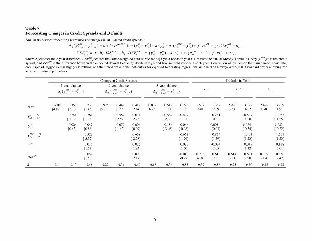
51  

Table 7 Forecasting Changes in Credit Spreads and Defaults

Annual time-series forecasting regressions of changes in BBB-rated credit spreads:

, ,( ) ( ) ( ) .BBB G EDF G G G BBB G HY HY

L t k L t k t Lt St St Lt Lt t t t kk y y a b ISS c y y d y e y y f rx g DEF u

1 2 ( ) ( ) ,HY EDF HY G G G BBB G HY

t k t t Lt St St Lt Lt t t kDEF a b ISS b DEF c y y d y e y y f rx u

where Δk denotes the k-year difference, denotes the issuer-weighted default rate for high yield bonds in year from the annual Moody’s default survey, yBBB-yG is the credit spread, and ISSEDF is the difference between the expected default frequency decile of high and low net debt issuers in each year. Control variables include the term spread, short-rate, credit spread, lagged excess high yield returns, and the time-t default rate. t-statistics for k-period forecasting regressions are based on Newey-West (1987) standard errors allowing for serial correlation up to k-lags.

Change in Credit Spreads Defaults in Year:

1-year change

, 1 , 11 ( )BBB G

L t L ty y

2-year change

, 2 , 22 ( )BBB G

L t L ty y

3-year change

, 3 , 33 ( )BBB G

L t L ty y

t+1 t+2 t+3

EDFISS 0.609 0.352 0.237 0.925 0.449 0.419 0.879 0.519 0.296 1.502 1.352 2.990 3.322 2.488 3.269 [4.07] [2.26] [1.45] [5.33] [1.85] [2.14] [6.25] [1.81] [1.05] [2.48] [2.39] [3.53] [4.62] [1.78] [1.91]

, ,G GL t S ty y -0.244 -0.280 -0.582 -0.631 -0.562 -0.427 0.281 -0.827 -1.063

[-1.39] [-1.75] [-2.59] [-2.23] [-2.36] [-1.91] [0.41] [-1.20] [-1.25]

,GS ty 0.024 0.042 -0.070 0.004 -0.156 -0.066 0.005 -0.084 -0.033

[0.43] [0.86] [-1.62] [0.09] [-3.46] [-0.98] [0.03] [-0.34] [-0.22]

, ,BBB GL t L ty y -0.523 -0.668 -0.663 0.824 1.401 1.501

[-3.32] [-2.78] [-1.76] [1.39] [1.23] [1.53] HYtrx 0.010 0.025 0.020 -0.084 0.048 0.128

[1.53] [1.34] [-1.50] [-2.05] [1.12] [2.01]

HYDEF 0.052 0.093 -0.013 0.786 0.618 0.614 0.681 0.359 0.538 [1.50] [2.17] [-0.27] [4.08] [2.31] [3.53] [2.90] [2.04] [2.47]

R2 0.11 0.17 0.45 0.22 0.36 0.60 0.18 0.36 0.55 0.37 0.56 0.25 0.30 0.13 0.22

 

52  

Table 8 Intermediary Balance Sheets and Issuer Quality

This table explores the relationship between ISSEDF and measures of intermediary balance sheet strength Z. The first two columns in each panel report the coefficient on Zt from regressions of the form

( ) ( ) .t k

EDF G G G BBB G HY

t t Lt St St Lt Lt ta b Z uISS c y y d y e y y f rx

Columns (3) to (6) report the coefficients on ISSEDF and Zt from return forecasting regressions of the form

2 2( ) ( ) ,HY

t t

EDF G G G BBB G HY

t t Lt St St Lt Lt trx a b ISS b Z uc y y d y e y y f rx

where rxHY denotes the 2-year excess return on high yield bonds. The regressions alternately omit ISSEDF, and include the term spread, short-rate, credit spread, and lagged excess high yield returns as controls. Measures of intermediary balance sheet strength, summarized in Table 1, include insurer equity capital E/A (total assets minus liabilities all over assets) and balance sheet growth dA/A (year-over-year percentage change in total assets); broker dealer equity capital E/A and balance sheet growth dA/A; bank equity capital E/A and balance sheet growth dA/A; lagged equal weighted returns on bank stocks based on Fama and French 48-industry classifications; and bank loan loss provisions scaled by total loans and leases. t-statistics for 2-year forecasting regressions are based on Newey-West (1987) standard errors allowing for serial correlation up to 2 lags.

Depvar: ISSEDF Depvar:

2

HY

trx

(1) (2) (3) (4) (5) (6)

Insurer Balance Sheets ISSEDF -13.102 -14.251 [-3.41] [-3.69]

E/AInsurer 0.156 0.133 -4.104 -2.058 -1.336 0.563 [3.58] [2.54] [-3.78] [-1.68] [-0.76] [0.33]

dA/AInsurer -0.008 -0.005 -0.382 -0.493 0.382 0.314 [-0.35] [-0.21] [-0.89] [-1.06] [0.70] [0.53]

Controls No Yes No No Yes Yes

R2 0.21 0.48 0.15 0.30 0.33 0.45

Broker-Dealer Balance Sheets ISSEDF -16.006 -14.579 [-5.25] [-4.20] E/ABD -0.017 -0.018 0.160 -0.105 -0.025 -0.289 [-0.98] [0.86] [0.31] [-0.27] [-0.04] [-0.55] dA/ABD -0.005 -0.003 -0.008 -0.088 -0.035 -0.080 [-1.60] [-1.06] [-0.08] [-0.96] [-0.49] [-1.58] Controls No Yes No No Yes Yes R2 0.06 0.42 0.00 0.28 0.32 0.46

Bank Balance Sheets ISSEDF -14.032 -13.648 [-4.28] [-4.81] E/ABank -0.013 -0.032 -0.558 -0.734 -0.208 -0.642 [-0.40] [-0.96] [0.50] [0.88] [-0.15] [-0.51] dA/ABank 0.036 0.019 -1.285 -0.780 -0.768 -0.512 [1.48] [0.71] [-2.64] [-1.60] [-1.58] [-1.04] Controls No Yes No No Yes Yes R2 0.07 0.43 0.12 0.32 0.35 0.47

Lagged Bank Stock Returns ISSEDF -13.927 -13.165 [-4.19] [-3.73] RBank,t-3,t 0.005 0.004 -0.105 -0.039 -0.068 -0.018 [2.54] [3.36] [-3.60] [-1.18] [-2.40] [-0.50] Controls No Yes No No Yes Yes R2 0.16 0.50 0.09 0.27 0.35 0.45

Bank Loan Loss Provisions ISSEDF -13.594 -13.913 [-4.30] [-4.42] LoanLosses -0.397 -0.139 10.182 4.783 1.777 -0.161 [-1.72] [-0.59] [2.00] [1.34] [0.36] [-0.05] Controls No Yes No No Yes Yes R2 0.14 0.41 0.10 0.28 0.32 0.45

 

53  

Table 9 Determinants of Issuer Quality

Time-series regressions of issuer quality ISSEDF on levels and past changes of interest rates:

1( )EDF G G G HY HY

t St Lt St t t tISS a b y c y y d rx e DEF u , or 1 1( ) .G G G HY HY

k k St k Lt St t k t k t k t

EDFt rxISS a b y c y y d e DEF u

yS

G denotes the short-term Treasury bill yield; yLG-yS

G denotes the term spread, DEFHY is the issuer-weighted high yield default rate from Moody’s, rLHY-rL

G is the excess high yield return, and Δk denotes the k-year difference. In columns (1) to (5) we regress the level of ISSEDF on a number of covariates, columns (6) to (10) repeat this analysis in first differences, and columns (11) to (15) in second differences. In the last two columns in each block we add additional controls for lagged stock market returns and macroeconomic variables (the growth in industrial product, real consumption growth, and a recession indicator). Robust t-statistics are shown in brackets.

ISSEDF 1ISSEDF 2ISSEDF (1) (2) (3) (4) (5) (6) (7) (8) (9) (10) (11) (12) (13) (14) (15)

Levels: ,

G

S ty -0.047 -0.036 -0.035 -0.026 [-1.63] [-1.22] [-1.14] [-0.99]

( )G G

Lt Sty y -0.277 -0.233 -0.218 -0.204 [-4.91] [-3.41] [-2.98] [-2.61]

1

HY

trx 0.014 0.015 0.009 0.016 [1.57] [2.78] [1.42] [3.14]

t

DEF -0.076 -0.013 -0.017 -0.010 [-3.11] [-0.59] [-0.68] [-0.40]

1-year ,1

G

S ty -0.107 -0.072 -0.073 -0.078

Changes: [-2.41] [-1.65] [-2.04] [-2.58]

1 ( )G G

Lt Sty y -0.335 -0.173 -0.165 -0.137 [-5.99] [-2.74] [-2.71] [-2.05]

1

HY

trx 0.031 0.025 0.014 0.018 [6.60] [5.00] [2.24] [3.25]

1 tDEF -0.043 -0.025 -0.031 -0.020

[-1.74] [-1.11] [-1.36] [-1.11]

2-year 2

G

Sty -0.134 -0.062 -0.061 -0.084

Changes: [-3.31] [-1.94] [-1.70] [-1.92]

2 ( )G G

Lt Sty y -0.410 -0.164 -0.154 -0.168 [-7.63] [-2.52] [-2.11] [-1.53]

3 1

HY

t trx 0.036 0.027 0.019 0.018

[6.91] [4.47] [2.17] [2.65]

2 tDEF

-0.065 -0.049 -0.064 -0.083 [-3.77] [-2.72] [-2.78] [-2.45]

Other controls None None None LaggedMKT

MacroVars

None None None  LaggedMKT

MacroVars

None None None LaggedMKT

MacroVars

R2 0.44 0.34 0.53 0.55 0.61 0.36 0.49 0.55 0.62 0.74 0.47 0.59 0.62 0.64 0.75