ISSN 1868-3967, Volume 1, Number 1 - Princeton …castlelab.princeton.edu/html/Papers/Enders-Dynamic...

This article was published in the above mentioned Springer issue.The material, including all portions thereof, is protected by copyright;all rights are held exclusively by Springer Science + Business Media.

The material is for personal use only;commercial use is not permitted.

Unauthorized reproduction, transfer and/or usemay be a violation of criminal as well as civil law.

ISSN 1868-3967, Volume 1, Number 1

Energy Syst (2010) 1: 31–59DOI 10.1007/s12667-009-0006-5

O R I G I NA L PA P E R

A dynamic model for the failure replacementof aging high-voltage transformers

Johannes Enders · Warren B. Powell · David Egan

Received: 26 May 2009 / Accepted: 14 December 2009 / Published online: 4 January 2010© Springer-Verlag 2009

Abstract As the electric transmission system in the U.S. ages, mitigating the risk ofhigh-voltage transformer failures becomes an increasingly important issue for trans-mission owners and operators. This paper introduces a model that supports theseefforts by optimizing the acquisition and the deployment of high-voltage transform-ers dynamically over time. We formulate the problem as a Markov Decision Processwhich cannot be solved for realistic problem instances. Instead we solve the prob-lem using approximate dynamic programming using three different value functionapproximations, which are compared against an optimal solution for a simplified ver-sion of the problem. The methods include a separable, piecewise linear value func-tion, a piecewise linear, two-dimensional approximation, and a piecewise linear func-tion based on an aggregated inventory that is shown to produce solutions within a fewpercent with very fast convergence. The application of the best performing algorithmto a realistic problem instance gives insights into transformer management issues ofpractical interest.

1 Introduction

In the 1960’s and 70’s, the electric power industry underwent a major expansion re-quiring a significant investment in high-voltage transformers. This investment hasproduced an age distribution with a bubble of older transformers that will beginfailing at a higher than average rate. We consider the problem faced by PJM In-terconnections, the largest regional transmission operator in the U.S. responsible for

J. Enders · W.B. Powell (�)Department of Operations Research and Financial Engineering, Princeton University, Princeton,USAe-mail: [email protected]

D. EganPJM Interconnection, Norristown, USA

Author's personal copy

mailto:[email protected]

32 J. Enders et al.

controlling the flow of energy through the electric power grid covering states fromNew Jersey, New York, Pennsylvania and Maryland through Ohio and Illinois. In thispaper we focus on high-voltage transformers that step up and down the voltage be-tween the backbone transmission system operating at 500 kV and the lower voltagetransmission system operating at 230 kV. Currently, approximately 50 percent of thehigh-voltage transformers in PJM’s transmission grid are 30 or more years old. Thetransformers can cost $5 million each, and require one to two years for delivery.

It is important to maintain a reliable set of transformers since the cost of a fail-ure can be quite high. If a transformer fails, the network incurs costs by needing topurchase energy from more expensive utilities to avoid a bottleneck. These costs canrange from several million to as high as $100 million per year. For an industry whichoperates with very thin profit margins, it is necessary to plan a replacement strategythat strikes a careful balance between potential congestion costs and equipment re-placement costs. Given capacity constraints on the industry which makes this equip-ment, it is necessary to design time-dependent safety stocks to respond to potentialfailures.

Our model optimizes transformer purchasing and deployment over time takinginto account failure uncertainty which changes with time. The model can be used tosupport the capital investment and risk mitigation planning performed by regionaltransmission organizations and transmission owners. There are two important trade-offs that we capture with this model:

• The model balances the minimization of adverse system effects due to failuresagainst the efficient use of financial resources. This is the acquisition problem.

• Once a replacement transformer is purchased there is the need to weigh its useto replace a failure now against a possible but uncertain use for a more importantfailure later. This is the deployment problem.

Such a model can be framed as a special case of an inventory problem. In thelanguage of inventory problems the safety stock of replacement transformers is the“inventory” and failures are “demands.” The transformer acquisition and deploymentmodel is an inventory problem with the following four characteristics. (1) Any un-served demand is fully backlogged. (2) There is a multi-period lead time. (3) Theinventory serves multiple demand classes, characterized by different shortage costs.(4) The demand process is fairly complex: demands are state dependent and corre-lated.

We only considered the possibility of replacing transformers that have failed. Thisis not a fundamental limitation of the model or algorithm. We can handle such asituation by using a rule to designate a transformer as “at risk” (a type of failure) withno congestion cost (but a higher risk of incurring congestion costs). But the reality isthat failure tails are extremely long. A high risk transformer can easily last another10 years, and inventories of spares are going to be sparse given the high capital cost.The decision to swap out an aging but working transformer would be based primarilyon issues of risk rather than expected cost.

Figure 1 shows a schematic representation of the transformer acquisition and de-ployment model at time t . To the left of the dashed line in the figure is the state of themodel before decisions at time t . To the right is the state of the model after decisions


A dynamic model for the failure replacement of aging high-voltage 33

Fig. 1 Schematicrepresentation of the transformeracquisition and deploymentmodel

at time t which we denote tx . Arrows represent decisions. At time t transformers ininventory can be used to meet a failure or be held in inventory to be available the nexttime period. If a failure is not met it remains part of the state. The circles representthe pipeline of ordered transformers that are due to arrive to the system in one, two,three, and four periods. High-voltage transformers are not the only domain wheresuch a model can be applied. It is generally applicable to spare provisioning for cap-ital intensive failure prone equipment with long lead times such as jet engines andship turbines.

Modeling transformer acquisition and deployment as a dynamic stochastic op-timization problem is fundamentally different from the approach that is currentlybeing taken by transmission owners. The strategy currently used in practice seeks aspare inventory level such that the expected time between spare shortages is big-ger than a threshold value. This approach does not make the cost trade-offs ex-plicit, and nor does it optimize them. The current approach does not provide in-sight into deployment decisions and does not consider that failure rates change overtime.

Backlogging and long lead times are standard features of inventory models. Zip-kin [27] gives a thorough account of these topics. It is well known that lead timesthat are longer than a single period introduce the “curse of dimensionality” into aninventory model. The state of the system needs to track not only how much inventoryis available and on order but also when ordered inventory is scheduled to arrive. Thisfact leads to a high-dimensional state variable.

The fact that there are multiple demand classes gives rise to the deployment prob-lem described above. When is it desirable to backlog lower priority failures in orderto have more replacement transformers available for uncertain future high priorityfailures? The pioneering work in inventory rationing is Topkis [24] who introducesa model with n demand classes, backlogging, and non-stationary demand distribu-tions. This model is to this date the closest match in the inventory rationing literatureto the system in this paper. Other contributions to the inventory rationing problem


34 J. Enders et al.

with backlogging include Deshpande et al. [7], De Véricourt et al. [6], Tempelmeier[22], and Ha [10]. The number of demand classes is large in our model because thesubstation locations have widely varying congestion costs. This contributes to the“curse of dimensionality” in our model.

The failure probability of a transformer in operation depends on its age and phys-ical condition. Therefore these attributes need to be part of the system state whichintroduces further complexity. Failures are also correlated due to the existence oftransformer banks. A bank is a set of transformers that always operate together. Oncea transformer in a bank fails, the entire bank shuts down and no further failures inthe same bank are possible. This correlation complicates the computation of expec-tations, such as expected congestion costs.

The issue of transformer spares has received some attention in the literature.Chowdhury and Koval [5] and Kogan et al. [12] develop procedures to determine theoptimal number of spares in a static model that assumes a stationary failure processand that all failures have the same priority. Li et al. [14] go beyond the previouslymentioned papers as they allow failure events of different priorities and also considerthe timing of spare additions. Their approach is rather cumbersome as it does notuse any optimization, requires the enumeration and evaluation of all possible fail-ure events, and needs to be repeated whenever the underlying transformer populationchanges. Our approach uses a realistic model of the physical system, which we solvein a compact way using approximate dynamic programming (ADP).

There is a larger literature on the management of spare parts, although transform-ers tend to be fairly unique given their size and cost. Simão and Powell [21] useapproximate dynamic programming to handle high-value spare parts for an aircraftmanufacturer which shares some of the same characteristics (and where we use asimilar approach). Wong et al. [25] and Wong et al. [26] propose heuristic policiesfor multi-item spare parts in the presence of lateral transshipments. Huiskonen [11]provides a nice discussion of the issues surrounding maintenance spare parts, but per-haps the most thorough modern discussion is [15] which considers in depth the useof inventory policies adapted to the management of spare parts, motivated by militaryapplications.

In this paper we propose a series of solution algorithms based on dynamic pro-gramming and approximate dynamic programming. The contributions of this paperare twofold: (1) We show that the use of separable, piecewise linear approximations,which has proven to be successful in prior work [8, 23] does not work for this prob-lem class. (2) We introduce two classes of non-separable approximations and show,through comparisons against the exact solution of a simplified MDP, that they pro-duce results between 0 and 4 percent of optimal.

In Sect. 2 we introduce notation and formulate the problem as a multi-period sto-chastic optimization model. Section 3 discusses the general algorithmic approachand Sect. 4 specifies the value function approximations and the ADP algorithms. InSect. 5 we describe the numerical work performed to validate the algorithm and anapplication of our best performing algorithm to a real high-voltage transformer pop-ulation.



2 Model formulation

A transformer is described by a vector of attributes a consisting of the elements

⎛⎜⎜⎜⎜⎜⎜⎜⎜⎝

substation idbank idphasefailedage

conditionavailability time

⎞⎟⎟⎟⎟⎟⎟⎟⎟⎠

.

An example of an attribute vector a is

a =

⎛⎜⎜⎜⎜⎜⎜⎜⎜⎝

Branchburg52A

false39.5

average0

⎞⎟⎟⎟⎟⎟⎟⎟⎟⎠

.

Each transformer in operation belongs to a substation identified by a substation iden-tifier. A substation contains one or more transformer banks and a bank is identified bya bank id. Within a bank a particular transformer is identified by the power phase thatit handles; current moves in one of three power phases, which are denoted A, B, or C.Another attribute indicates if a transformer has failed or not. The failure probabilityover a time interval depends on the age and the condition of the transformer. The ageis measured in time periods and the condition can be “good,” “average,” or “watch.”All the attributes described so far are needed to model transformers in operation. Oneattribute that is important for replacement transformers is the estimated time of ar-rival, since transformers have to be ordered 12 to 24 months in advance. We refer tothe time when a transformer is scheduled to arrive as the available time. An availabletime of 0 indicates that the transformer is available to be used as a replacement.

We let A be the set of all possible attribute vectors. For this research, we need toseparate transformers that are in operation (that is, in working order), and transform-ers that have failed and are in need of replacement. The sample attribute vector abovedescribes a transformer that is in working order. An example of an attribute vectorfor a transformer that is not in working order is

a =

⎛⎜⎜⎜⎜⎜⎜⎜⎜⎝

–––

false0

good3

⎞⎟⎟⎟⎟⎟⎟⎟⎟⎠

,


36 J. Enders et al.

where “–” denotes a missing attribute. To separate transformers that are in operation(in working order) and failed transformers that are in need of replacement, we define

Arep = set of attribute vectors for transformers that can be used as replacements,

Aop = set of attribute vectors for transformers in operation,

Afail = set of attributes vectors for transformers that have already failed,

A = Aop ∪ Arep = set of transformer attribute vectors, a ∈ A.

We need to represent attributes of transformers that have failed. For this purpose, wedefine

af = attribute vector of a failed transformer after we have acted on the trans-former d to replace it.

We define

as = attribute vector of replacement transformers that are s periods away frombeing available,

τ = scalar lead time, giving the number of months that a transformer has tobe ordered in advance.

We note that as is a particular instance of an attribute vector for a transformer thatwill arrive in s time periods. There can be a number of attribute vectors describingtransformers that are s time periods away. We use this notation to indicate the valueof the time at which a transformer will become available. All the replacement trans-formers have attributes in the set {a0, a1, . . . , aτ−1} = Arep. a0 is the attribute vectorof a replacement transformer with age 0, that has not failed, is in “good” condition,and has availability time 0, i.e. is in inventory. aτ−1 is the attribute vector of a trans-former that has just been ordered. aτ is the attribute vector of a transformer that hasnot been purchased but is available for purchase. Note that aτ is not an element ofArep.

We now introduce the notation for the system state measured immediately beforethe decisions at time t are made. This is called the pre-decision state.

Rta = number of transformers with attribute vector a at time t before the timet decisions are made,

Rt = (Rta)a∈A = vector of pre-decision transformers at time t .

Throughout the paper we will also use the state captured immediately after the deci-sions at time t are made. We use the notation

Rxt = (Rx

ta)a∈A = vector of post-decision transformers at time t .

Transformers can be acted upon with three decision types:

Drep = set of types of decisions to use a replacement transformer in inventoryto replace a type of transformer that has failed and is in need of repair.The set contains one decision da for each transformer that can be usedfor replacements, a ∈ Arep,

db = decision to buy a replacement transformer,



d∅ = decision to hold a replacement transformer in inventory to the nextperiod.

For example, imagine that we have three failed transformers at different locations,with different attributes. Denote these by a, a′ and a′′. The set Drep would includethe decisions da, da′ and da′′ representing the decision to replace the transformer withattribute a, a′ or a′′, respectively.

We define the set of all possible types of decisions using

D = Drep ∪ db ∪ d∅.

The decision variables and their contributions are defined as:

xtad = number of transformers with attribute a to be acted on with decision d

at time t ,xt = (xtad)a∈A,d∈D = decision vector at time t ,

xrept = (xtad)a∈Arep,d∈Drep = vector of replacement decisions at time t .

The one period contribution function of our model is

ctad = cost of acting on one unit of resource with attribute a with decision d

at time t ,Ct(xt ) = ctaτ dbxtaτ db − ∑

d∈Drep cta0dxta0d + cta0d∅xta0d

∅ .

The first term constitutes the purchase cost of new replacement transformers. Thesecond term is avoided congestion costs for each failure for which the model pro-vides a replacement transformer. The third term is an inventory holding cost chargedfor all transformers in inventory that are held from one period to the next. We notethat congestion costs depend on the number of failed transformers. In practice, thenumber of failed transformers is very small, since utilities manage their networksvery conservatively.

Randomness enters the system through random transformer failures and randomtransitions from “good” to “average” and from “average” to “watch.” A random eventalways produces one more transformer of a certain type and one less transformer ofanother type, for example, one more failed transformer and one less working trans-former. We denote

Rta = the change in the number of transformers with attribute vector a due torandom events during period t , and

Rt = (Rta)a∈A = vector of random changes during time t .

In any given period a working transformer that is in use at a substation can fail, changecondition, or remain unaffected by randomness. Each of these events happens with acertain probability which depends on the age of the transformer and its condition. Thefailure probability also depends on the status of the other transformers in the bank. Ifone transformer of a bank failed then the other transformers in the same bank cannotfail until the failed transformer is replaced. This dependence arises from the fact thata single transformer failure will cause the entire bank to be shut down. And if a bankis shut down no further failures in that bank can occur.


38 J. Enders et al.

The transition from Rt to Rxt is described by the transition equations

Rxtaτ−1

= xtaτ db , (1)

Rxtas

= Rtas+1 for s ∈ {1, . . . , τ − 2}, (2)

Rxta0

= xta0d∅ + Rta1 , (3)

Rxtaf = Rtaf − xta0d for af ∈ Aop, d ∈ Drep. (4)

Equation (1) models the decision to purchase a transformer. Equation (2) models thetransition of a transformer that has not yet arrived from being τ time periods awayto τ − 1 time periods away. Equation (3) models the accumulation of transformersin inventory, and (4) models the decision to repair a transformer. The post- to pre-decision transition function simply is

Rt+1 = Rxt + Rt+1. (5)

Since the model is a multi-period model under uncertainty we wish to find an optimalpolicy, π , and the corresponding decision rule, Xπ(Rt ) that returns optimal decisionsas a function of the system state Rt . The optimization problem is to find

minπ

E

{T∑

t=0

γ tCt (Xπ(Rt ))

}, (6)

where γ is a discount factor. Our challenge now is to find a good replacement policy,something that we do with approximate dynamic programming.

3 Algorithmic approach

Stochastic integer programming algorithms have been developed to solve discrete op-timization problems under uncertainty. One approach is to formulate the problem as alarge-scale deterministic (mixed) integer program, the deterministic equivalent. Par-ija et al. [18] and Ahmed et al. [1] solve the deterministic equivalent directly. Parijaet al. [18] show that taking into account special problem structure results in algo-rithms that are more efficient than a straightforward application of a general purposeMIP solver. At the same time this work shows that solving the deterministic equiv-alent is computationally infeasible for the transformer acquisition and deploymentmodel. The largest problem solved in Parija et al. [18] has 18,006 binary variables,3 time periods, and 500 scenarios. We will be solving the transformer model for upto 200 time periods which would result in much larger deterministic problems.

Another computational approach to solving stochastic integer programs uses de-composition. All major work has been on two-stage problems [3, 13, 17] and doesnot directly apply to the multi-stage transformer problem.

The starting point for our computational strategy is the classic dynamic program-ming recursion

Vt(Rt ) = minxt∈Xt (Rt )

{C(xt ) + γ E[Vt+1(Rt+1)]|Rt }, (7)



where

Xt = feasible region at time t ,Vt+1(Rt+1) = value function—expected discounted cumulative costs for time

periods t + 1, t + 2, . . . , T .

This recursion cannot be solved using classic backward dynamic programmingbecause of the dimensionality of the problem. The long lead time for replacementtransformers increases the dimensionality as does the backlogging of failures of vary-ing importance and the fact that transformer age and condition are part of the attributevector.

The algorithmic approach taken in this paper is approximate dynamic program-ming (ADP) [2, 19]. This algorithmic strategy has recently been applied with successto large-scale, complex optimization problems under uncertainty [19]. We solve thedynamic program approximately by estimating a value function approximation recur-sively using Monte Carlo simulation. We use the following notation:

Vt (Rxt ) = approximation of value function Vt (R

xt ).

In order to solve the problem using a Monte Carlo based technique we need a re-cursion that can be solved for a single sample realization of the random informationprocess at time t . Equation (7) cannot be used for this purpose as the knowledge ofa time t + 1 sample realization, Rt+1(ω), at time t would violate non-anticipativity.In order to overcome this problem we formulate the following recursion around thepost-decision state:

Vt−1(Rx

t−1

) = E

[min

xt∈Xt (Rt )

{C(xt ) + γVt

(Rx

t

)}](8)

where Xt is defined by the following constraints:

xtad∅ +∑

d∈Drep

xta0d = Rta0 , (9)

Rxt,aτ−1

− xt,a−τdb = 0, (10)

Rxta0

− xtad∅ = Rta1 , (11)

xta0d ≤ Rtaf for d ∈ Drep, (12)

xtad ≥ 0 ∀a, d. (13)

Here, (9) enforces flow conservation given current inventories. Equation (10) definesthe in-transit inventory in terms of the amount ordered, while (11) defines the newinventory as the sum of what was left over plus new arrivals. Equation (12) limits thenumber of decisions to replace transformers by the number of transformers that havefailed, and (13) provides the necessary non-negative constraints.

The recursion in (8) can be solved approximately by using an approximation ofthe value function. The corresponding approximate problem is

V nt

(R

x,nt−1, Rt (ω

n)) = V n

t

(Rn

t

) = minxt∈Xt (R

nt )

{C(xt ) + γ V n−1

t

(R

x,nt

)}(14)


40 J. Enders et al.

Step 0. Initialize V 0t (Rx

t ) for t ∈ {0,1, . . . , T }.Step 1. Set n = 1 and t = 0.Step 2. Solve problem (14) and transition function as in (1)–(4).Step 3. Sample Rt+1(ωn) and transition function as in (5).Step 4. If t < T , set t = t + 1, and go to Step 2.Step 5. Update V n−1

t (Rxt ) for t ∈ {0,1, . . . , T − 1}.

Step 6. If n < N set n = n + 1, t = 0, and got to Step 2.

Fig. 2 Sketch of approximate dynamic programming algorithm for the transformer acquisition and de-ployment model

where n ∈ {0,1, . . . ,N} is the iteration counter. Note that this optimization problemdoes not violate non-anticipativity because in order to make the time t decisions xt theformulation only uses the information that is indeed available at that time. The ideaof ADP is to produce a good approximation V N

t (Rxt ) which results in near optimal

decisions. Figure 2 gives a sketch of the ADP approach.Note that the algorithm steps forward in time. This avoids the enumeration of

states and actions that is typical for classic backward dynamic programming. Theuse of simulation avoids the need to evaluate the expectation explicitly. In the nextsection we introduce functional forms for Vt (R

xt ) and show how this function can be

estimated iteratively using Monte Carlo methods.The next section describes a family of value function approximations for solving

the dynamic program.

4 Value function approximations

We tested three different functional forms for Vt (Rxt ). The starting point is a separa-

ble piecewise linear function that has been used successfully in Topaloglu and Powell[23], Powell et al. [20], and Godfrey and Powell [8]. We will show that this functionis inappropriate in our problem setting and explain why. The second functional formextends the first approach by using pre-decision state information. The third algo-rithm uses an explicit two-dimensional, piecewise linear value function approxima-tion (VFA). We show how to estimate a two-dimensional value function surface.

4.1 Piecewise linear separable value function approximation

Topaloglu and Powell [23], Powell et al. [20], and Godfrey and Powell [8] all show themerits of a VFA that is separable in the elements of the resource vector Rx

t . Recallingthat the set Afail is the attributes of transformers that have already failed (these are thedemands that we need to satisfy), we can approximate the value of all transformers(failed and replacements held in inventory) using a separable approximation of theform

Vt

(Rx

t

) =∑

a∈Arep

Vta

(Rx

ta

) +∑

a∈Afail

Vta

(Rx

ta

). (15)

The first term on the right hand side is the value derived from replacement trans-formers and the second term is the value of deferring the replacement of a failed



transformer. We follow the methods in Topaloglu and Powell [23] and use piecewiselinear approximations for the value of each type of transformer.

Let us focus on replacement transformers first. Since there can be multiple replace-ment transformers ordered and in inventory, we choose piecewise linear functionswith integer breakpoints to represent the value of such replacement transformers.These piecewise linear functions have to be convex to reflect the decreasing marginalvalue of additional resources of the same type.

Note that the purchase decision produces a newly purchased transformer aτ−1and the holding decision is associated with transformers a0. The corresponding valuefunction components Vta0(R

xta0

) and Vtaτ−1(Rxtaτ−1

) are of particular importance be-cause they are related to decisions. All the intermediate transformers are not subjectto decision making. In fact we introduce an algorithm that only requires the estima-tion of Vta0(R

xta0

) and Vtaτ−1(Rxtaτ−1

).We now turn to failed transformers, the second term on the right hand side of (15).

There is future value associated with replacing a failure, namely avoiding the con-gestion costs that the failure would have caused in the future. The VFA componentassociated with replacing a failure is the expected future congestion cost savings.Figure 3 illustrates the subproblem at time t using piecewise linear VFA componentsfor replacement transformers in the future, and linear VFA components for the valueof replacing a failure. The nodes labeled a4, . . . , a1 represents transformers that are4, . . . ,1 time periods away from being used. The value of transformers at each ofthese nodes, and at the inventory node, is captured by a piecewise linear value func-tion. In addition, there are linear functions capturing the value of covering a failedtransformer which depends on the congestion cost.

Fig. 3 Schematic representation of the piecewise-linear separable VFA for the transformer acquisitionand deployment model


42 J. Enders et al.

With the VFA described above problem (14) becomes an easily solvable linearprogram. Using the notation

M = number of segments of a piecewise linear VFA component,ytam = variable representing the mth segment of the piecewise linear VFA

Vta(Rxta),

yt = (ytam)a∈{a0,aτ−1},t∈{0,...,T } = vector of variables representing piecewiselinear VFAs,

vtam = slope of the mth segment of the piecewise-linear VFA.

The problem is to solve

Vt (Rt ) = minxt ,yt

{C(xt ) + γ

( ∑d∈Drep

vtaf xta0d +∑

a∈{aτ−1,a0}

M∑m=1

vtamytam

)}(16)

subject to

xta0d∅ +

∑d∈Drep

xta0d = Rta0 , (17)

Rxtaτ−1

− xtadb = 0, (18)

Rxta0

− xtad∅ = Rta1 , (19)

M∑m=1

ytam − Rxta = 0 for a ∈ {aτ−1, a0}, (20)

xta0d ≤ Rtaf for d ∈ Drep, (21)

0 ≤ ytam ≤ 1 for a ∈ {aτ−1, a0}, m = 1, . . . ,M, (22)

xtad ≥ 0 ∀a, d. (23)

The minimization problem in (16) includes the one-period costs in C(xt ), and thevalue function approximation that captures the impact of decisions on the future.These impacts include a linear approximation of the downstream cost of not replac-ing a failed transformer now, and a piecewise-linear approximation of the value ofreplacement transformers. Equation (17) is the flow conservation constraint for trans-formers that can be acted on now. Equation (18) defines the post-decision resourcestate for transformers that are in-transit, while (19) defines the post-decision state fortransformers that are available now. Equation (20) defines the sum of the variables(ytam), m = 1, . . . ,M , used in the piecewise linear value function, to be the totalnumber of transformers that are now available, while (21) is the demand constraintwhich limits our ability to replace failed transformers by the number of transformersthat have failed. Equation (22) limits the y variables to be between 0 and 1, and (23)imposes non-negativity.

In our numerical work we will provide the data showing that a separable VFA isinappropriate for our problem class. In this section we focus on providing intuition



why a separable approximation may not work. Figure 3 shows that the value con-tribution of a newly purchased spare aτ−1, Vtaτ−1(R

xtaτ−1

), is independent of all theother replacement transformers, Rx

ta0,Rx

ta1, . . . ,Rx

taτ−2. This is implied by separabil-

ity. This assumption is only true if there is no spare inventory holding over from oneperiod to the next. In our problem replacement transformers will typically be held ininventory for some time because congestion costs are substantially higher than inven-tory holding costs. In this case a spare that is in inventory or in the pipeline at time t

can easily still be around when a newly purchased spare arrives in inventory at timet + τ . The marginal value of one more or one less transformer of type aτ−1 at timet may very well depend on how many transformers Rx

ta0,Rx

ta1, . . . ,Rx

taτ−2are in the

system. If there is an abundance of spares in inventory and in the pipeline at timet then the value of ordering one more spare is probably low. If transformer inven-tory is exhausted the value of ordering one more spare is probably higher. We needa VFA that captures this behavior while retaining the computational advantages ofproblem (16)–(23). The next section introduces such an approximation as well as acomplete ADP algorithm.

4.2 Piecewise linear VFA with pre-decision state information

For computational purposes it is desirable to maintain the network LP structure ofproblem (16)–(23). To this end we define

Rt = max

(τ−1∑s=0

Rtas −∑

a∈Afail

Rta,0

). (24)

In this equation, Rt is capturing the total number of transformers that are either intransit or available to be assigned.

We have Rt ≈ ∑τ−1s=0 Rx

taswhere the approximation is an equality unless the model

is holding back available spare inventory from low-priority failures. This approxima-tion allows us to replace the VFA component Vtaτ−1(R

xtaτ−1

) with Vtaτ−1(Rxtaτ−1

+ Rt )

without destroying the network structure of problem (16)–(23). Making the changeonly requires calculating Rt and adding it as a supply to the node representing Rx

taτ−1.

Figure 4 gives an example of the procedure. In problem (16)–(23) only (18) changesto

Rxtaτ−1

− xtaτ db = Rt . (25)

With the optimization problem solved we turn to the issue of estimating the pa-rameters vta , the slopes of Vt (R

xt ). We simplify this task by setting the linear value

function components of the failures to a fixed multiple of the one-period congestioncosts in the various locations. We denote

vtaf = ρf ctaf d ∀d ∈ Drep (26)

where

ρf = tunable parameter that penalizes the value of not satisfying a failure at aparticular point in time.


44 J. Enders et al.

Fig. 4 Schematic representation of the piecewise-linear VFA with pre-decision state information for thetransformer acquisition and deployment model

Fixing the linear VFA components that capture the value of pushing a failure to thefuture allows us to focus on the piecewise-linear VFA components representing thevalue of replacement transformers.

The estimation of the piecewise-linear value functions is done in an iterative pro-cedure where each iteration consists of stepping forward through the time horizon,simulating a sample path, and solving the following approximate problem. Using n

to denote the iteration index the approximate problem (16)–(23) becomes:

V nt

(Rn

t

) = min{xt ,yt }∈X ′′

t

{C(xt ) + γ

( ∑d∈Drep

vtaf xta0d +∑

a∈{aτ ,a0}

M∑m=0

vntamytam

)}(27)

where X ′′t is the feasible region defined by (17), (25), and (19)–(23). By solving per-

turbations of (27) with respect to Rnt we can obtain stochastic sample gradients that

represent a sample realization of the value of one more or one less replacement trans-former. Let ea be a vector of zeros and a one at element a. We define the stochasticright gradient as

v+,nta0

= V nt

(Rn

t + ea0

) − V nt

(Rn

t

), (28)

and the left stochastic gradient as

v−,nta0

= V nt

(Rn

t

) − V nt

(Rn

t − ea0

)if Rn

ta0> 0. (29)

Note that we only calculate stochastic gradients for replacement transformers in in-ventory (attribute vector a0). This is because these transformers are the only source



of (additional) rewards. In that sense the replacement transformers in inventory drivethe system. The stochastic gradients are sample realizations of value function slopesand need to be smoothed into the current estimates of the slopes in order to “average”across sample paths. Which slope estimates should be updated with v

+,nta0

and v−,nta0

?Since a stochastic gradient is the value of one more or one less transformer in inven-tory at time t , the gradients need to update the value functions that lead to one moreor one less transformer in inventory at time t .

To obtain one more or one less transformer in inventory at time t the model wouldhave to hold one more transformer in inventory at time t − 1 or order one moretransformer at time t − τ . Therefore v

+,nta0

and v−,nta0

update V n−1t−1,a0

and V n−1t−τ,aτ−1

.The stochastic gradients at time t are passed backwards in time to the VFAs thatprovide transformer spares for time t . V n−1

t−1,a0and V n−1

t−τ,aτ−1share the same role as

the mechanism for providing spares for time t but they are not the same functions.The difference lies in what segments of the VFAs components are updated by thestochastic gradients.

Updating the VFA components V n−1t−τ,aτ−1

and V n−1t−1,a0

is a two-step procedure.

We pick V n−1t−τ,aτ−1

to illustrate the steps. In the first step the stochastic gradients aresmoothed into the current value function estimate in the following way to obtain anintermediate vector of slopes (un

t−τ,aτ−1,m)m=0,1,...,M . The calculation is

unt−τ,aτ−1,m

=

⎧⎪⎨⎪⎩

(1 − αn−1)vn−1t−τ,aτ−1,m

+ αn−1v+,nta0

if m = Rx,nt−τ,aτ−1

+ Rt ,

(1 − αn−1)vn−1t−τ,aτ−1,m

+ αn−1v−,nta0

if m = Rx,nt−τ,aτ−1

+ Rt − 1,

vn−1t−τ,aτ−1

otherwise,(30)

where αn−1 is a step size between 0 and 1. Equation (30) updates the slopes ofour piecewise linear approximation using the right (v+,n

ta0) and left (v+,n

ta0) derivatives

around the current number of transformers. At this stage, we only update the slopesadjacent to the number of transformers currently in a particular state.

Unfortunately, this computation can cause convexity violations. To restore con-vexity we apply the convexity restoring procedure of Godfrey and Powell [9] to theintermediate vector of slopes (un

t−τ,aτ−1,m)m=0,1,...,M . The updated value function

slopes are obtained as

V nt−τ,aτ−1

= (vnt−τ,aτ−1,m

)m=0,1,...,M

= �(un

t−τ,aτ−1,m

)m=0,1,...,M

(31)

where � is the convexity restoring operator defined by the equations

minvnt−τ,aτ−1

∥∥vnt−τ,aτ−1

− unt−τ,aτ−1

∥∥2 (32)

subject to:

vnt−τ,aτ−1,m+1 − vn

t−τ,aτ−1,m≥ 0 for m = 0, . . . ,M − 1. (33)

The idea of ADP is that after a finite number of iterations, N , the VFA V Nt is a

good approximation of the true value function for every t and that the collection ofall value functions across time implies a policy that is close to optimal.


46 J. Enders et al.

Step 0. Initialize V 0t for t = 1, . . . , T and set n = 1.

Step 1. Do for t = 0, . . . , T − 1:Step 1a. Calculate Rn

t as in (24) and solve time t subproblem (27). Store Rnt and R

x,nt for later use.

Step 1b. Calculate sample gradients as in (28) and (29) and store them for later use.Step 1c. Sample Rn

t+1(ωnt+1) and calculate Rn

t+1 as in (5).

Step 2a. For t = τ, . . . , T − 1 calculate V nt−τ,aτ−1

(Rx,nt−τ,aτ−1

+ Rnt−τ t ) = (vn

t−τ,aτ−1,m)m=0,1,...,M us-ing (30) and (31).

Step 2b. For t = 1, . . . , T − 1 calculate V nt−1,a0

(Rx,nta0

) = (vnt−1,a0,m

)m=0,1,...,M using

unt−1,a0,m =

⎧⎪⎪⎨⎪⎪⎩

(1 − αn−1)vn−1t−1,a0,m

+ αn−1v+,nta0

if m = Rx,nt−1,a0

,

(1 − αn−1)vn−1t−1,a0,m

+ αn−1v−,nta0

if m = Rx,nt−1,a0

− 1,

vn−1t−1,a0

otherwise

(34)

and(vnt−1,a0,m

)m=0,1,...,M

= �(unt−1,a0,m

)m=0,1,...,M

. (35)

Step 3. Set n = n + 1. If n < N , go to Step 1.

Fig. 5 ADP training algorithm for the replacement transformer acquisition and deployment model

Step 0. Set n = 1.Step 1. Do for t = 0, . . . , T − 1:Step 1a. Calculate Rn

t as in (24) and solve time t subproblem (27).Step 1b. Sample Rn

t+1(ωnt+1) and calculate Rn

t+1 as in (5).Step 2. Set n = n + 1. If n < N , go to Step 1.

Fig. 6 Evaluation algorithm for the replacement transformer acquisition and deployment model

Figure 5 gives the complete ADP algorithm for estimating the VFA. Equations(34) and (35) are analogous to (30) and (31) for the inventory value functions Vta0 .Once the VFA estimation is accomplished running the model involves executing asimplified version of Fig. 5. We call this the evaluation algorithm because this al-gorithm is used to evaluate policies based on a number of sample paths. Figure 6specifies the steps of the evaluation algorithm with fixed VFAs.

4.3 Two-dimensional piecewise linear VFA

Given the non-separable nature of the value function V (Rxt ) the thought of a multi-

dimensional non-separable VFA is attractive. In this section we explore this ideafor the two-dimensional case. The two-dimensional case is particularly interestingin our problem setting because it allows us to capture the joint future value of ac-quisition and holding decisions. We present an algorithm to estimate a VFA surface,Vt (R

xta0

,Rxta1

). Such a VFA would allow us to express the true relationship betweenresource states and their value if we restrict the problem to two dimensions, which inour application means we are restricting the problem to a two-period lead time.



To minimize notational clutter let us denote Rxta0

by y1 and Rxta1

by y2. GivenMi ∈ N0 for i = 1,2, let I = {0,1, . . . ,M1}, J = {0,1, . . . ,M2} and define

Y 1k = {y = (y1, y2)|y1 = [0,M1], y2 = k} ∀k ∈ J ,

Y 2l = {y = (y1, y2)|y1 = l, y2 = [0,M2]} ∀l ∈ I,

to be the horizontal and vertical grid lines in the rectangle (0,0), (0,M2), (M1,M2),(M1,0). Let

G =M2⋃k=0

Y 1k ∪

M1⋃l=0

Y 2l ,

be the grid itself and

V = [0,1, . . . ,M1] × [0,1, . . . ,M2],the set of vertices in G . We define Vt : G → R. We assume Vt is submodular on V andpiecewise-linear convex with integer breakpoints along each grid line. Submodularitymeans that the slopes in the y2 direction are increasing along the y1 dimension andthe slopes in the y1 direction are increasing along the y2 dimension. Formally, thedefinition of submodularity is

Vt (y1, y2 + 1) − Vt (y1, y2) ≤ Vt (y1 + 1, y2 + 1) − Vt (y1 + 1, y2).

Submodularity can be thought of as a form of convexity for discrete functions. For adetailed discussion of submodularity, see [16].

Figure 7 gives an example of the function Vt . As can be seen, we are taking advan-tage of the natural convexity (expressed as submodularity) of this function. It capturesthe interaction between acquisition and holding decisions in a non-separable function,allowing us to test the errors introduced using a separable approximation.

Fig. 7 Example of function Vt


48 J. Enders et al.

Fig. 8 Illustration of V nt in

terms of its slopes on the gridlines

We show how to solve problem (14) using the VFA defined here. To simplifynotation let V n

tij = V nt (i, j). Define

v1,ntij = V n

tij − V nt,i−1,j , i ∈ I \ 0, j ∈ J ,

v2,ntij = V n

tij − V nt,i,j−1, i ∈ I, j ∈ J \ 0,

the slopes of V nt along the grid lines. Figure 8 illustrates V n

t in terms of its slopes.The problem is

V nt

(Rn

ta0,Rn

ta1

) = minxt ,yt

{C(xt ) + γ

(Vt00 + V 1

t

(x

rept

) + V 2t (y1, y2)

)}, (36)

with

V 1t =

∑d∈Drep

vta0dxta0d , (37)

V 2t =

M1∑i=1

v1,n−1t i0 yt1i +

M2∑j=1

v2,n−1t0j yt2j +

M1∑i=1

M2∑j=1

(v

2,n−1t ij − v

2,n−1t,i−1,j

)yt1iyt2j , (38)

subject to

xta0d∅ +

∑d∈Drep

xta0d = Rnta0

, (39)

y2 − xtaτ db = 0, (40)

y1 − xta0d∅ = Rn

ta1, (41)

xta0d ≤ Rntaf for d ∈ Drep, (42)

∑i∈I

y1i − y1 = 0, (43)



∑j∈J

y2j − y2 = 0, (44)

xtad ≥ 0 ∀a ∈ A, d ∈ D (45)

y1i , y2j ∈ {0,1} ∀i ∈ I, j ∈ J . (46)

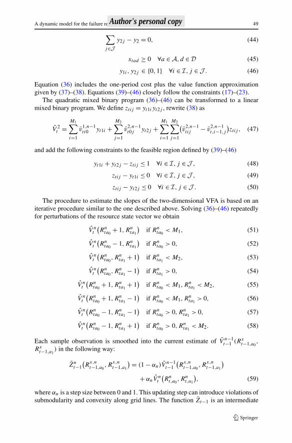
Equation (36) includes the one-period cost plus the value function approximationgiven by (37)–(38). Equations (39)–(46) closely follow the constraints (17)–(23).

The quadratic mixed binary program (36)–(46) can be transformed to a linearmixed binary program. We define ztij = yt1iyt2j , rewrite (38) as

V 2t =

M1∑i=1

v1,n−1t i0 yt1i +

M2∑j=1

v2,n−1t0j yt2j +

M1∑i=1

M2∑j=1

(v

2,n−1t ij − v

2,n−1t,i−1,j

)ztij , (47)

and add the following constraints to the feasible region defined by (39)–(46)

yt1i + yt2j − ztij ≤ 1 ∀i ∈ I, j ∈ J , (48)

ztij − yt1i ≤ 0 ∀i ∈ I, j ∈ J , (49)

ztij − yt2j ≤ 0 ∀i ∈ I, j ∈ J . (50)

The procedure to estimate the slopes of the two-dimensional VFA is based on aniterative procedure similar to the one described above. Solving (36)–(46) repeatedlyfor perturbations of the resource state vector we obtain

V nt

(Rn

ta0+ 1,Rn

ta1

)if Rn

ta0< M1, (51)

V nt

(Rn

ta0− 1,Rn

ta1

)if Rn

ta0> 0, (52)

V nt

(Rn

ta0,Rn

ta1+ 1

)if Rn

ta1< M2, (53)

V nt

(Rn

ta0,Rn

ta1− 1

)if Rn

ta1> 0, (54)

V nt

(Rn

ta0+ 1,Rn

ta1+ 1

)if Rn

ta0< M1,R

nta1

< M2, (55)

V nt

(Rn

ta0+ 1,Rn

ta1− 1

)if Rn

ta0< M1,R

nta1

> 0, (56)

V nt

(Rn

ta0− 1,Rn

ta1− 1

)if Rn

ta0> 0,Rn

ta1> 0, (57)

V nt

(Rn

ta0− 1,Rn

ta1+ 1

)if Rn

ta0> 0,Rn

ta1< M2. (58)

Each sample observation is smoothed into the current estimate of V n−1t−1 (Rx

t−1,a0,

Rxt−1,a1

) in the following way:

Znt−1

(R

x,nt−1,a0

,Rx,nt−1,a1

) = (1 − αn)Vn−1t−1

(R

x,nt−1,a0

,Rx,nt−1,a1

)

+ αnVnt

(Rn

t,a0,Rn

t,a1

), (59)

where αn is a step size between 0 and 1. This updating step can introduce violations ofsubmodularity and convexity along grid lines. The function Zt−1 is an intermediate


50 J. Enders et al.

Step 0. Initialize V 0t for t = 1, . . . , T and set n = 1.

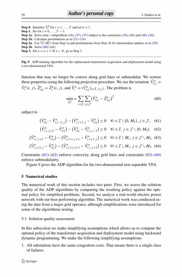
Step 1. Do for t = 0, . . . , T − 1:Step 1a. Solve time t subproblem (36), (37), (47) subject to the constraints (39)–(46) and (48)–(50).Step 1b. Calculate perturbations as in (51)–(54).Step 2a. Use V n

t (Rnt ) from Step 1a and perturbations from Step 1b for intermediate updates as in (59).

Step 2b. Solve (60)–(64)Step 3. Set n = n + 1. If n < N , go to Step 1.

Fig. 9 ADP training algorithm for the replacement transformer acquisition and deployment model usinga two-dimensional VFA

function that may no longer be convex along grid lines or submodular. We restorethese properties using the following projection procedure. We use the notation: V n

tij =V n

t (i, j), Zntij = Zn

t (i, j), and V nt = (V n

tij )i∈I,j∈J . The problem is

minV n

t

=∑i∈I

∑j∈J

(V n

tij − Zntij

)2 (60)

subject to(V n

tij − V nt,i−1,j

) − (V n

t,i+1,j − V ntij

) ≤ 0 ∀i ∈ I \ {0,M1}, j ∈ J , (61)(V n

t,i,j+1 − V ntij

) − (V n

tij − V nt,i,j−1

) ≤ 0 ∀i ∈ I, j ∈ J \ {0,M2}, (62)(V n

t,i,j+1 − V ntij

) − (V n

t,i+1,j+1 − V nt,i+1,j

) ≤ 0 ∀i ∈ I \ M1, j ∈ J \ M2, (63)(V n

t,i+1,j − V ntij

) − (V n

t,i+1,j+1 − V nt,i,j+1

) ≤ 0 ∀i ∈ I \ M1, j ∈ J \ M2. (64)

Constraints (61)–(62) enforce convexity along grid lines and constraints (63)–(64)enforce submodularity.

Figure 9 gives the ADP algorithm for the two-dimensional non-separable VFA.

5 Numerical studies

The numerical work of this section includes two parts. First, we assess the solutionquality of the ADP algorithms by comparing the resulting policy against the opti-mal policy for simplified problems. Second, we analyze a real-world electric powernetwork with our best-performing algorithm. The numerical work was conducted us-ing the data from a major grid operator, although simplifications were introduced forsome of the algorithmic testing.

5.1 Solution quality assessment

In this subsection we make simplifying assumptions which allows us to compute theoptimal policy of the transformer acquisition and deployment model using backwarddynamic programming. We make the following simplifying assumptions:

1. All substations have the same congestion costs. That means there is a single classof failures.



Table 1 Characteristics of test data sets

Data Lead time Expected Holding Discount Initial Max. Max.

set (periods) failures cost factor inventory inventory order

($ million)

A1 2 2 0.5 0.9 6 6 4

A2 4 2 0.5 0.9 11 11 3

A3 6 2 0.5 0.9 12 12 3

A4 8 2 0.5 0.9 12 12 3

B1 2 4 2 0.9 10 10 6

B2 4 4 2 0.9 14 14 5

B3 6 4 2 0.9 15 15 5

B4 8 4 2 0.9 32 – –

C1 2 1 0.1 0.098465 2 5 3

C2 4 1 0.1 0.098465 4 8 3

C3 6 1 0.1 0.098465 6 11 3

C4 8 1 0.1 0.098465 8 12 3

D1 2 4 0.1 0.098465 12 14 8

D2 4 4 0.1 0.098465 18 20 7

D3 6 4 0.1 0.098465 24 – –

D4 8 4 0.1 0.098465 33 – –

E1 2 2 0.1 0.098465 6 8 5

E2 4 2 0.1 0.098465 12 14 4

E3 6 2 0.1 0.098465 16 16 4

E4 8 2 0.1 0.098465 19 19 3

2. No backlogging. Failures that are not immediately met are lost to the system.3. The number of failures per period is a binomial random variable with fixed para-

meters.

In our test data sets we hold the following parameters constant: the number oftime periods is 40, the failure probability of a single transformer is 0.2, the pur-chase cost is $5 million, and the congestion cost parameter is $20 million. Note thatthe congestion cost parameter includes current period congestion costs ($5 million)and expected future congestion costs ($15 million, ρf = 3). The test data sets havevarying lead times, holding costs, discount factors, and sizes of the transformer pop-ulation. For each data set we specify an initial transformer inventory which in mostcases is enough to cover failures until new purchases become available. A maximuminventory and the maximum order size are chosen such that the state space is mini-mized without cutting off an optimal solution. Table 1 summarizes the different testdata sets.

The data sets are chosen such that it is feasible in most cases to calculate theoptimal policy using backward dynamic programming (BDP). We use this optimal


52 J. Enders et al.

Step 0. Initialize state space R and value function VT (RxT

) for all RxT

∈ R.Step 1. Do for t = T , . . . ,1:Step 2. Do for each Rx

t−1 ∈ R:Step 3. Compute Vt−1(Rx

t−1) = E[minxt {C(xt ) + γVt (Rxt )}].

Step 4. Next Rxt−1.

Step 5. Next t .

Fig. 10 BDP training algorithm for the replacement transformer acquisition and deployment model

Fig. 11 Evaluation of three stepsize rules

solution to compare against ADP based on the following three VFAs: piecewise linearseparable (PLS) of Sect. 4.1, piecewise linear with pre-decision state information(PLPRE) of Sect. 4.2, and two-dimensional (2D) of Sect. 4.3.

A challenge of the BDP algorithm is to make sure that the underlying model ex-actly matches the model in (8). This is best achieved by using a BDP that uses a valuefunction around the post-decision state variable. Figure 10 gives the BDP algorithmthat we use.

In order to determine the number of iterations, N , and the step size rule, αn, forthe PLS and PLPRE algorithms we performed the following analysis. Choosing thestep size rule αn = 1

nwe ran the PLPRE algorithm on data set E2 varying the number

of iterations in the set {5,15,25,50,100,200,300,400}. The resulting VFAs wereevaluated based on 100 sample paths. We repeated the analysis for the step size rulesαn = 5

4+n, αn = 20

19+n. Figure 11 summarizes the results of this analysis. Based on

these results we chose the step size rule αn = 2019+n

and N = 200. Figure 11 indicatesthat the PLPRE algorithm converges nicely as the number of training iterations in-creases. We used this approximation as our test bed for determining the best stepsizerule, which is influenced primarily by the overall level of uncertainty and how long atransformer is held in inventory.



Table 2 Numerical results comparing PLPRE and PLS with optimal (BDP). “–” indicate that the BDP didnot complete due to memory constraints (2 GB). All experiments are run on a single processor (Intel P4),3.06 GHz machine

Data BDP PLPRE PLS

set time rPLPREBDP 95% CI Time rPLS

BDP 95% CI rPLSPLPRE Time

(s) (%) (%) (s) (%) (%) (%) (s)

A1 0 −0.1 [−0.7,0.6] 595 9.9 [7.4,12.4] 10.0 565

A2 1 1.5 [0.9,2.1] 580 5.7 [3.7,7.6] 4.1 597

A3 22 4.1 [3.3,4.9] 598 4.8 [3.1,6.6] 0.7 575

A4 285 3.4 [2.8,4.1] 541 2.4 [1.5,3.2] −1.0 581

B1 0 0.7 [0.3,1.2] 604 8.0 [6.2,9.9] 7.2 559

B2 10 2.9 [2.2,3.6] 793 1.7 [1.0,2.5] −1.1 472

B3 504 3.2 [2.5,3.8] 816 1.0 [0.4,1.5] −2.1 372

B4 – – – 778 – – −2.4 386

C1 0 −0.2 [−0.5,0.1] 775 18.3 [15.2,21.4] 18.6 354

C2 1 0.9 [−0.1,1.8] 788 11.7 [9.2,14.3] 10.8 360

C3 13 1.9 [0.6,3.1] 828 10.3 [7.7,12.8] 8.2 375

C4 146 3.0 [1.5,4.4] 869 7.7 [5.4,10.1] 4.6 376

D1 0 1.3 [0.8,1.7] 873 15.8 [13.1,18.5] 14.4 370

D2 54 2.8 [2.0,3.7] 906 12.5 [10.0,15.0] 9.4 371

D3 – – – 852 – – 3.7 362

D4 – – – 762 – – 4.7 375

E1 0 1.1 [0.5,1.6] 680 16.2 [13.5,19.0] 15.0 356

E2 2 0.7 [0.2,1.1] 696 12.6 [10.0,15.3] 11.9 361

E3 102 0.7 [0.2,1.1] 709 11.5 [8.9,14.1] 10.8 360

E4 454 1.6 [0.7,2.6] 719 6.3 [4.4,8.1] 4.5 368

To compare the different ADP algorithms against optimal we use the followingperformance metric

rij = Average cost of algorithm i policy

Average cost of algorithm j policy− 1.

Averages are based on 100 sample paths that do not change between algorithms.Table 2 shows the computational results comparing the PLS, PLPRE and the optimalBDP algorithm. We see that PLS, which assumes separability, does not work wellin almost all cases. The few cases where PLS performs better than or comparable toPLPRE (A3, A4, B2, B3) are characterized by longer lead times and high holdingcosts. PLPRE performs consistently well and both algorithms have very reasonablerun times. We also see that BDP does not scale well: some of the small problems usedin this section were too big to be solved to optimality.

The two-dimensional algorithm (2D) can only be applied without modifications toproblems with two-period lead times and we restrict our analysis to these cases. We


54 J. Enders et al.

Table 3 Size of the VFA and computational results for the 2D algorithm

Data r2DBDP (%) Time (s)

set 100 500 1000 2000 4000 100 500 1000 2000 4000

iter. iter. iter. iter. iter. iter. iter. iter. iter. iter.

A1 46.1 3.1 2.7 3.6 2.5 367 2415 5673 12,875 28,581

B1 70.6 4.2 2.0 1.2 1.5 417 2891 7671 19,789 29,393

C1 77.8 3.5 3.6 3.9 3.0 316 1961 4064 8,817 15,610

D1 218.8 109.5 20.7 4.4 1.5 572 3510 9142 28,277 80,876

E1 154.7 11.7 2.7 1.7 1.8 348 2376 5512 14,155 35,018

run the 2D algorithm for 100, 500, 1000, 2000, and 4000 iterations which gives usan idea of the convergence behavior for different data sets. Generally, convergence isslower than for PLPRE which prompts the need for larger step sizes. The step size of

choice is αn =√

1 − ( nN

)2 which declines slowly for most of the iterations and has

the added benefit that it does not have a parameter requiring fine tuning.Table 3 shows the results for the 2D algorithm. We see that the 2D algorithm pro-

duces good policies but shows slower convergence behavior than PLPRE and muchhigher run times. What drives the run times aside from the higher number of iterationsis the choice of M1 and M2 which determines the size of the linear mixed integer pro-gram. The number of binary variables ranges from 77 for the smallest data set C1 to230 for the biggest problem D1. Also note that the mixed integer program is solvedup to nine times per iteration and time period in order to obtain all V n

t .Since the PLPRE outperforms 2D we make PLPRE our algorithm of choice for

the policy study in the following section.

5.2 Transformer acquisition and deployment policies for PJM’s network

We use the ADP algorithm to analyze the high-voltage transformer population ofPJM Interconnection, a major regional transmission organization. PJM controls theelectric power grid in a large area of the Eastern U.S. PJM’s transmission system in-cludes 182 500–230 kV transformers in 42 substations. These are the transformers ofinterest for this study. In each period the outcome of a Bernoulli experiment indicateswhether a particular working transformer has failed or not. The failure probabilitiesfor the experiment are obtained from hazard rate curves that give the failure proba-bility as a function of the transformer age. These curves are estimated by PJM basedon historical failure data and certain assumptions on the shape of the curve (see [4]).There is one hazard rate curve for every transformer condition (“good,” “average,”“watch”). Figure 12 gives a general idea of the shape of the hazard rate curves. Thecondition attribute transitions randomly following a discrete Markov chain. Failuresare correlated in the sense that a bank can only have one failed transformer at a time.

We analyze the system over a 50-year horizon using 3-month time periods. Thelead time is 6 time periods (1.5 years). The transformer purchase cost is $5 mil-lion. The congestion costs vary greatly across substations, ranging from less than



Fig. 12 Examples of hazardrate curves used for failuregeneration

Fig. 13 Average cost of theADP policy over the entire50-year horizon as a function ofthe number of training iterations

$0.25 million to more than $50 million per period. Congestion costs, which are care-fully computed by PJM, capture the increase in power generation costs when PJMhas to use energy from a more expensive utility in order to avoid bottlenecks in thegrid created by transformer failures. Congestion costs are computed as the incremen-tal cost from a single transformer failure. Of course, if there are multiple transformerfailures, interactions in the network imply that the cost of two failures may be greaterthan the sum of the congestion costs for individual failures. However, failures arerare, which means that using constant congestion costs is a reasonable first-order ap-proximation. For our experiments, we used a congestion cost multiplier ρf = 3 andan inventory holding cost of $75,000 per period (1.5 percent of purchase costs). Allcosts grow over time at a rate of 1.5 percent per time period to reflect inflation.

We evaluate the ADP policy over 100 sample paths. The algorithmic parametersthat need to be chosen are the number of training iterations, N , and the step sizerule αn. The step size rule of choice is αn = 20

19+nbased on the analysis in the previous

subsection. In order to determine the appropriate number of iterations we evaluate thepolicy on 100 sample paths after 5, 15, 25, 50, 100, 200, and 300 training iterations.Figure 13 shows no improvement after iteration 100. We therefore choose N = 100.

Figure 14 shows the average number of failures per year that result from followingthe ADP policy. We observe the pronounced “bubble” reflecting the failure of theolder transformer cohorts that are currently in operation. The expected number of


56 J. Enders et al.

Fig. 14 Average number oftransformer failures per yearover 50-year time horizon

Fig. 15 Fraction of substationtransformer failures that arereplaced without delay

failures increases by 50 percent over the next 15 years, then remains high for another15 years and declines afterwards. Figure 15 lists all 42 substations in descendingorder of congestion costs. The figure shows what fraction of the failures in each



Table 4 Sensitivity analysis for different parameter scenarios. Scenarios are listed in order of ascendingtotal costs. τ is the lead time parameter and ρf is the congestion cost multiplier. Costs are aggregate valuesover the entire 50-year horizon and averaged over 100 sample paths. +/− columns list the relative costchange in percent compared to the base case which is indicated by *

τ ρf Purch. +/− Cong. +/− Inv. holding +/− Total

(periods) (periods) cost (%) cost (%) cost (%) ($ mil)

($ mil) ($ mil) ($ mil)

4 3 996 0 81 −18 66 −7 1143

6 5 1012 +1 57 −41 82 +17 1151

6* 3 998 − 98 − 70 − 1166

8 3 1003 +1 126 +29 77 +9 1206

6 1 981 −2 303 +208 54 −23 1338

substation are met immediately at the end of the period when they happened. A validmodel with the given parameter settings should make sure that failures in substationswith the highest congestion costs are always met without any delay. This is whatthe figure shows. We also see that delays routinely occur when failures happen inthe substations with the lowest congestion costs. This is what we expect given themodel’s inventory deployment feature and the widely varying congestion costs. Dueto this feature the model incurs delays in serving low-priority failures in order toavoid uncertain future delays serving high-priority failures.

We vary the lead time parameter and the congestion cost multiplier in order toperform sensitivity analysis. The effect of changing lead times is of interest as leadtimes can vary depending on the state of the transformer manufacturing industry. Thecongestion cost multiplier is the key parameter to control inventory levels and the riskof delays. Starting with the base case we study the effect of one parameter at a time.The left side of Table 4 shows the 5 scenarios we analyze.

First note that the purchasing costs are almost constant across all scenarios. Re-ducing the lead time saves money, both in terms of congestion costs and inventoryholding costs. Increasing the congestion cost multiplier leads to more conservativeinventory policies that lead to lower congestion costs at the expense of higher in-ventory holding costs. Increasing lead times result in cost increases. The policy forthis scenario leads to higher inventory levels and therefore inventory holding costs.Interestingly the congestion costs also increase considerably despite higher inventorylevels. Apparently, the higher inventory levels do not compensate for the additionaluncertainty that the lead time increase introduces into the model. Finally, a lowercongestion cost multiplier leads to very aggressive inventory policies that result invery high congestion costs.

Table 5 shows inventory levels and the relative frequency of running out of sparesfor the congestion cost multiplier scenarios. These numbers are calculated by look-ing at the results of the 100 evaluation iterations. As the reward for meeting a failuregrows (increasing ρf ) the model adopts a more conservative policy leading to higherinventory levels and a lower shortage frequency. Even with the most conservative in-ventory policies the probability of running out of spares in any three month periodis 1.7 percent. Note the connection between the relative shortage frequency in Ta-


58 J. Enders et al.

Table 5 ρf is the congestioncost multiplier. The base case isindicated by *. The inventorystatistic is averaged across all200 time periods and all 100sample paths, so the sample sizeis 20,000

ρf Average inventory Relative frequency of

(periods) (# of transformers) “more failures than spares”

1 4.6 0.1236

3* 5.7 0.0358

5 6.51 0.017

ble 5 and the immediate coverage ratio in Fig. 15. Figure 15 considers delays dueto shortages and intentional delays due to holding back inventory. The frequency inTable 5 only considers shortages and it also does not distinguish by substation. It isimportant to note that the inventory deployment feature will make sure that inventoryshortages tend to affect lower-priority failures before they affect higher-priority ones.In other words, with an overall shortage frequency of 1.7 percent the likelihood thathigh-priority failures will be affected is much closer to 0.

6 Conclusions

We have introduced the spare transformer acquisition and deployment model whichwe solved using ADP. Our computational evidence shows that standard piecewise-linear separable value functions do not work in this problem setting. This observationis expected to generalize to similar problems in capital intensive industries wherelead times are long and the shortage costs by far outweigh inventory holding costs.This paper introduces two novel value function approximation strategies which resultin near optimal policies on a variety of test data sets. The PLPRE algorithm is alsocomputationally efficient. Our analysis of a real power transmission system indicatesthat the expected number of transformer failures per time period will gradually rise by50 percent over the course of the next 15 years. With an optimal replacement policythere will be considerable delays in meeting low-priority failures. Longer lead timesincrease congestion costs and inventory holding costs. With high inventory levelsshortages are expected to occur 1.7 percent of the time.

In the current analysis the location of replacement transformers is not considered.Allowing replacement transformers to be stored at the substations would be an exten-sion of the current model and a worthy topic of future research.

References

1. Ahmed, S., King, A.J., Parija, G.: A multi-stage stochastic integer programming approach for capacityexpansion under uncertainty. J. Glob. Optim. 26, 3–24 (2003)

2. Bertsekas, D., Tsitsiklis, J.: Neuro-dynamic Programming. Athena Scientific, Belmont (1996)3. Caroe, C.C., Tind, J.: L-shaped decomposition of two-stage stochastic programs with integer recourse.

Math. Program. 83(3), 139–152 (1998)4. Chen, Q.M., Egan, D.M.: A Bayesian method for transformer life estimation using Perks’ hazard

function. IEEE Trans. Power Syst. 21(4), 1954–1965 (2006)5. Chowdhury, A.A., Koval, D.O.: Development of probabilistic models for computing optimal distrib-

ution substation spare transformers. IEEE Trans. Ind. Appl. 41(6), 1493–1498 (2005)



6. De Véricourt, F., Karaesmen, F., Dallery, Y.: Optimal stock allocation for a capacitated supply system.Manage. Sci. 48(11), 1486–1501 (2002)

7. Deshpande, V., Cohen, M.A., Donohue, K.: A threshold inventory rationing policy for service-differentiated demand classes. Manage. Sci. 49(6), 683–703 (2003)

8. Godfrey, G., Powell, W.: An adaptive dynamic programming algorithm for dynamic fleet manage-ment, I: Single period travel times. Transp. Sci. 36, 21–39 (2002)

9. Godfrey, G.A., Powell, W.B.: An adaptive, distribution-free approximation for the newsvendor prob-lem with censored demands, with applications to inventory and distribution problems. Manage. Sci.47, 1101–1112 (2001)

10. Ha, A.Y.: Stock-rationing policy for make-to-stock production system with two priority classes andbackordering. Nav. Res. Logist. 44, 457–472 (1997)

11. Huiskonen, J.: Maintenance spare parts logistics: special characteristics and strategic choices. Int. J.Prod. Econ. 71, 125–134 (2001)

12. Kogan, V.I., Roeger, C.J., Tipton, D.E.: Substation distribution transformers failures and spares. IEEETrans. Power Syst. 11(4), 1905–1912 (1996)

13. Laporte, G., Louveaux, E.V.: The integer L-shaped method for stochastic integer programs with com-plete recourse. Oper. Res. Lett. 13, 133–142 (1993)

14. Li, W., Vaahedi, E., Mansour, Y.: Determining number and timing of substation spare transformersusing a probabilistic cost analysis approach. IEEE Trans. Power Deliv. 14(3), 934–939 (1999)

15. Muckstadt, J.A.: Analysis and Algorithms for Service Parts Supply Chains. Springer, Berlin (2005)16. Nemhauser, G., Wolsey, L., Fisher, M.: An analysis of approximations for maximizing submodular

set functions—I. Math. Program. 14, 265–294 (1978)17. Norkin, V.I., Ermoliev, Y.M., Ruszczynski, A.: On optimal allocation of indivisibles under uncertainty.

Oper. Res. 46(3), 381–395 (1998)18. Parija, G.R., Ahmed, S., King, A.J.: On bridging the gap between stochastic integer programming and

MIP solver technologies. INFORMS J. Comput. 16(1), 73–83 (2004)19. Powell, W.B.: Approximate Dynamic Programming: Solving the Curses of Dimensionality. Wiley,

Hoboken (2007)20. Powell, W.B., Shapiro, J.A., Simão, H.P.: An adaptive dynamic programming algorithm for the het-

erogeneous resource allocation problem. Transp. Sci. 36, 231–249 (2002)21. Simão, H., Powell, W.: Approximate dynamic programming for management of high-value spare

parts. J. Manuf. Technol. Manag. 20, 147–160 (2009)22. Tempelmeier, H.: Supply chain inventory optimization with two customer classes in discrete time.

Eur. J. Oper. Res. 174, 600–621 (2005)23. Topaloglu, H., Powell, W.B.: Dynamic programming approximations for stochastic, time-staged inte-

ger multicommodity flow problems. INFORMS J. Comput. 18(1), 31–42 (2006)24. Topkis, D.M.: Optimal ordering and rationing policies in a non-stationary dynamic inventory model

with n demand classes. Manage. Sci. 15(3), 160–176 (1968)25. Wong, H., Van Houtum, G., Cattrysse, D., Van Oudheusden, D.: Simple, efficient heuristics for multi-

item multi-location spare parts systems with lateral transshipments and waiting time constraints.J. Oper. Res. Soc. 56, 1419–1430 (2005)

26. Wong, H., Van Houtum, G.J., Cattrysse, D., Oudheusden, D.V.: Multi-item spare parts systems withlateral transshipments and waiting time constraints. Eur. J. Oper. Res. 171, 1071–1093 (2006)

27. Zipkin, P.: Foundations of Inventory Management. McGraw-Hill, New York (2000)


ISSN 1868-3967, Volume 1, Number 1 - Princeton …castlelab.princeton.edu/html/Papers/Enders-Dynamic...

Documents

Transcript of ISSN 1868-3967, Volume 1, Number 1 - Princeton …castlelab.princeton.edu/html/Papers/Enders-Dynamic...