ISSN 1472-2739 (on-line) 1472-2747 (printed) ATG · PDF fileISSN 1472-2739 (on-line) 1472-2747...

ISSN 1472-2739 (on-line) 1472-2747 (printed) 337

Algebraic & Geometric Topology

ATGVolume 2 (2002) 337–370

Published: 21 May 2002

On Khovanov’s categorification of theJones polynomial

Dror Bar-Natan

Abstract The working mathematician fears complicated words but lovespictures and diagrams. We thus give a no-fancy-anything picture richglimpse into Khovanov’s novel construction of “the categorification of theJones polynomial”. For the same low cost we also provide some computa-tions, including one that shows that Khovanov’s invariant is strictly strongerthan the Jones polynomial and including a table of the values of Khovanov’sinvariant for all prime knots with up to 11 crossings.

AMS Classification 57M25

Keywords Categorification, Kauffman bracket, Jones polynomial, Kho-vanov, knot invariants

1 Introduction

In the summer of 2001 the author of this note spent a week at Harvard Univer-sity visiting David Kazhdan and Dylan Thurston. Our hope for the week wasto understand and improve Khovanov’s seminal work on the categorificationof the Jones polynomial [Kh1, Kh2]. We’ve hardly achieved the first goal andcertainly not the second; but we did convince ourselves that there is somethingvery new and novel in Khovanov’s work both on the deep conceptual level (notdiscussed here) and on the shallower surface level. For on the surface levelKhovanov presents invariants of links which contain and generalize the Jonespolynomial but whose construction is like nothing ever seen in knot theorybefore. Not being able to really digest it we decided to just chew some, andthen provide our output as a note containing a description of his construction,complete and consistent and accompanied by computer code and examples butstripped of all philosophy and of all the linguistic gymnastics that is necessaryfor the philosophy but isn’t necessary for the mere purpose of having a workingconstruction. Such a note may be more accessible than the original papers. Itmay lead more people to read Khovanov at the source, and maybe somebodyreading such a note will figure out what the Khovanov invariants really are.Congratulations! You are reading this note right now.

c© Geometry & Topology Publications

338 Dror Bar-Natan

1.1 Executive summary In very brief words, Khovanov’s idea is to replacethe Kauffman bracket 〈L〉 of a link projection L by what we call “the Khovanovbracket” JLK, which is a chain complex of graded vector spaces whose gradedEuler characteristic is 〈L〉. The Kauffman bracket is defined by the axioms

〈∅〉 = 1; 〈©L〉 = (q + q−1)〈L〉; 〈0〉 = 〈1〉 − q〈H〉.Likewise, the definition of the Khovanov bracket can be summarized by theaxioms

J∅K = 0 → Z → 0; J©LK = V ⊗ JLK; J0K = F(

0 → J1K d→ JHK{1} → 0

)

.

Here V is a vector space of graded dimension q + q−1 , the operator {1} is the“degree shift by 1” operation, which is the appropriate replacement of “multi-plication by q”, F is the “flatten” operation which takes a double complex toa single complex by taking direct sums along diagonals, and a key ingredient,the differential d, is yet to be defined.

The (unnormalized) Jones polynomial is a minor renormalization of the Kauff-man bracket, J(L) = (−1)n−qn+−2n−〈L〉. The Khovanov invariant H(L) is thehomology of a similar renormalization JLK[−n−]{n+ − 2n−} of the Khovanovbracket. The “main theorem” states that the Khovanov invariant is indeed alink invariant and that its graded Euler characteristic is J(L). Anything inH(L) beyond its Euler characteristic appears to be new, and direct computa-tions show that there really is more in H(L) than in its Euler characteristic.

1.2 Acknowledgements I wish to thank David Kazhdan and Dylan Thurstonfor the week at Harvard that led to writing of this note and for their help sincethen. I also wish to thank G. Bergman, S. Garoufalidis, J. Hoste, V. Jones,M. Khovanov, A. Kricker, G. Kuperberg, A. Stoimenow and M. Thistlethwaitefor further assistance, comments and suggestions.

2 The Jones polynomial

−

++

+

+

−

1 2

3

4 5

6

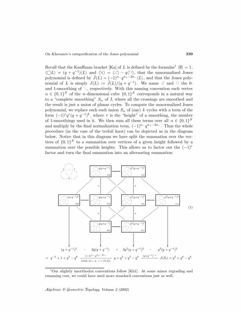
n+ = 4; n− = 2

All of our links are oriented links in an oriented Euclideanspace. We will present links using their projections to theplane as shown in the example on the right. Let L be alink projection, let X be the set of crossings of L, let n =|X |, let us number the elements of X from 1 to n in somearbitrary way and let us write n = n+ +n− where n+ (n−)is the number of right-handed (left-handed) crossings in X .(again, look to the right).

Algebraic & Geometric Topology, Volume 2 (2002)

On Khovanov’s categorification of the Jones polynomial 339

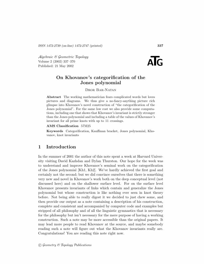
Recall that the Kauffman bracket [Ka] of L is defined by the formulas1 〈∅〉 = 1,〈©L〉 = (q + q−1)〈L〉 and 〈0〉 = 〈1〉 − q〈H〉, that the unnormalized Jonespolynomial is defined by J(L) = (−1)n−qn+−2n−〈L〉, and that the Jones poly-nomial of L is simply J(L) := J(L)/(q + q−1). We name 1 and H the 0-and 1-smoothing of 0, respectively. With this naming convention each vertexα ∈ {0, 1}X of the n-dimensional cube {0, 1}X corresponds in a natural wayto a “complete smoothing” Sα of L where all the crossings are smoothed andthe result is just a union of planar cycles. To compute the unnormalized Jonespolynomial, we replace each such union Sα of (say) k cycles with a term of theform (−1)rqr(q + q−1)k , where r is the “height” of a smoothing, the numberof 1-smoothings used in it. We then sum all these terms over all α ∈ {0, 1}X

and multiply by the final normalization term, (−1)n−qn+−2n− . Thus the wholeprocedure (in the case of the trefoil knot) can be depicted as in the diagrambelow. Notice that in this diagram we have split the summation over the ver-tices of {0, 1}X to a summation over vertices of a given height followed by asummation over the possible heights. This allows us to factor out the (−1)r

factor and turn the final summation into an alternating summation:

1

3

2 q(q+q−1)

100

CCCC

CCC

CCCC

CCC+

q2(q+q−1)2

110

DDDD

DDDD

DDDD

DDD

+

(q+q−1)2

000

||||||||||||||

DDDD

DDDD

DDDD

D

��

q(q+q−1)

010

{{{{{{{{{{{{{{{

EEEEEEEEE

EEEE

+

q2(q+q−1)2

101

+

q3(q+q−1)3

111

��

q(q+q−1)

001

yyyyyy

yyyyyy

��

q2(q+q−1)2

011

xxxxxxxxxxxxxx

��(q + q−1)2 − 3q(q + q−1) + 3q2(q + q−1)2 − q3(q + q−1)3

(1)

= q−2 + 1 + q2 − q6 ·(−1)n− qn+−2n−

−−−−−−−−−−−−−−→(with (n+, n−) = (3, 0))

q + q3 + q5 − q9 ·(q+q−1)−1

−−−−−−−→ J(&) = q2 + q6 − q8.

1Our slightly unorthodox conventions follow [Kh1]. At some minor regrading andrenaming cost, we could have used more standard conventions just as well.


340 Dror Bar-Natan

3 Categorification

3.1 Spaces

Khovanov’s “categorification” idea is to replace polynomials by graded vectorspaces2 of the appropriate “graded dimension”, so as to turn the Jones polyno-mial into a homological object. With the diagram (1) as the starting point theprocess is straight forward and essentially unique. Let us start with a brief onsome necessary generalities:

Definition 3.1 Let W =⊕

m Wm be a graded vector space with homogeneouscomponents {Wm}. The graded dimension of W is the power series qdim W :=∑

m qm dim Wm .

Definition 3.2 Let ·{l} be the “degree shift” operation on graded vectorspaces. That is, if W =

⊕

m Wm is a graded vector space, we set W{l}m :=Wm−l , so that qdim W{l} = ql qdim W .

Definition 3.3 Likewise, let ·[s] be the “height shift” operation on chain com-

plexes. That is, if C is a chain complex . . . → Cr dr

→ Cr+1 . . . of (possiblygraded) vector spaces (we call r the “height” of a piece Cr of that complex),and if C = C[s], then Cr = Cr−s (with all differentials shifted accordingly).

Armed with these three notions, we can proceed with ease. Let L, X , n and n±

be as in the previous section. Let V be the graded vector space with two basiselements v± whose degrees are ±1 respectively, so that qdim V = q+q−1 . Withevery vertex α ∈ {0, 1}X of the cube {0, 1}X we associate the graded vectorspace Vα(L) := V ⊗k{r}, where k is the number of cycles in the smoothing of Lcorresponding to α and r is the height |α| =

∑

i αi of α (so that qdim Vα(L)is the polynomial that appears at the vertex α in the cube at (1)). We then setthe rth chain group JLKr (for 0 ≤ r ≤ n) to be the direct sum of all the vectorspaces at height r : JLKr :=

⊕

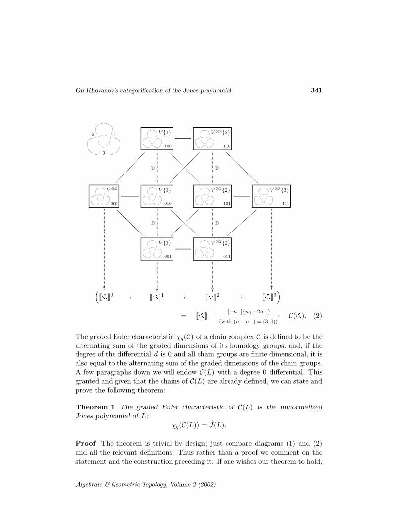
α:r=|α| Vα(L). Finally (for this long paragraph),we gracefully ignore the fact that JLK is not yet a complex, for we have not yetendowed it with a differential, and we set C(L) := JLK[−n−]{n+ − 2n−}. Thusthe diagram (1) (in the case of the trefoil knot) becomes:

2Everything that we do works just as well (with some linguistic differences) over Z.In fact, in [Kh1] Khovanov works over the even more general ground ring Z[c] wheredeg c = 2.



1

3

2 V {1}

100

>>>>

>>

>>>>

>>⊕

V ⊗2{2}

110

@@@@

@@@@

@@@@

@@

⊕

V ⊗2

000

��

????

????

????

��

V {1}

010

��

AAAA

AAAA

AAAA

⊕

V ⊗2{2}

101

⊕

V ⊗3{3}

111

��

V {1}

001

}}}}}}

}}}}}

��

V ⊗2{2}

011

|||||||||||||

��(

J&K0 ; J&K1 ; J&K2 ; J&K3)

= J&K ·[−n−]{n+−2n−}−−−−−−−−−−−−−−→(with (n+, n−) = (3, 0))

C(&). (2)

The graded Euler characteristic χq(C) of a chain complex C is defined to be thealternating sum of the graded dimensions of its homology groups, and, if thedegree of the differential d is 0 and all chain groups are finite dimensional, it isalso equal to the alternating sum of the graded dimensions of the chain groups.A few paragraphs down we will endow C(L) with a degree 0 differential. Thisgranted and given that the chains of C(L) are already defined, we can state andprove the following theorem:

Theorem 1 The graded Euler characteristic of C(L) is the unnormalizedJones polynomial of L:

χq(C(L)) = J(L).

Proof The theorem is trivial by design; just compare diagrams (1) and (2)and all the relevant definitions. Thus rather than a proof we comment on thestatement and the construction preceding it: If one wishes our theorem to hold,


342 Dror Bar-Natan

everything in the construction of diagram (2) is forced, except the height shift[−n−]. The parity of this shift is determined by the (−1)n− factor in thedefinition of J(L). The given choice of magnitude is dictated within the proofof Theorem 2.

3.2 Maps

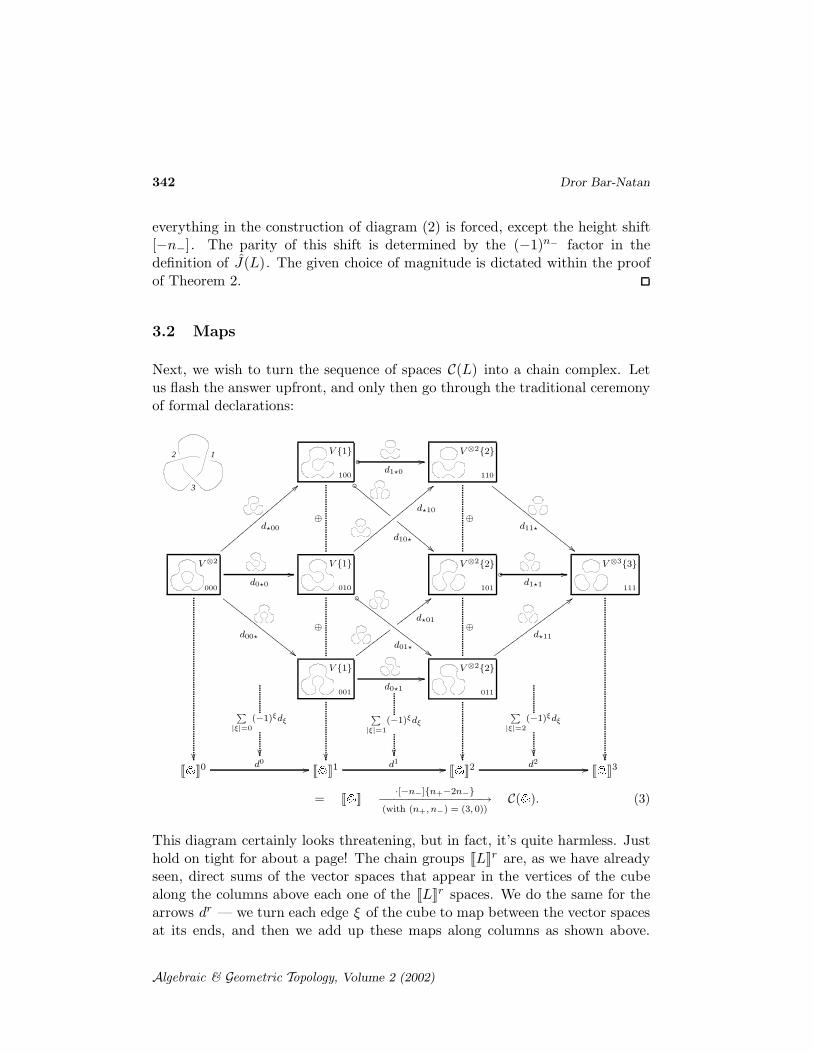
Next, we wish to turn the sequence of spaces C(L) into a chain complex. Letus flash the answer upfront, and only then go through the traditional ceremonyof formal declarations:

1

3

2 V {1}

100

◦d1⋆0

//

◦

EEEEEEEE

d10⋆

""EEEE

EEEE⊕

V ⊗2{2}

110

d11⋆

""FFFFFFFFFFFFFFFFFF

⊕

V ⊗2

000

d⋆00

==zzzzzzzzzzzzzzzzzz

d0⋆0

//

d00⋆

""FFFFFFFFFFF

FFFFF

��

V {1}

010

d⋆10

<<yyyyyyyyyyyyyyyyyy

◦

d01⋆##GGGGGGGGGGGGGGGG

⊕

V ⊗2{2}

101

◦d1⋆1

//

⊕

V ⊗3{3}

111

��

V {1}

001

wwwwwwww

d⋆01

;;wwwwwwww

d0⋆1

//

��

V ⊗2{2}

011

d⋆11

;;vvvvvvvvvvvvvvvvv

��J&K0 d0

// J&K1 d1// J&K2 d2

// J&K3

∑

|ξ|=0

(−1)ξdξ

��

∑

|ξ|=1

(−1)ξdξ

��

∑

|ξ|=2

(−1)ξdξ

��

= J&K ·[−n−]{n+−2n−}−−−−−−−−−−−−−−→(with (n+, n−) = (3, 0))

C(&). (3)

This diagram certainly looks threatening, but in fact, it’s quite harmless. Justhold on tight for about a page! The chain groups JLKr are, as we have alreadyseen, direct sums of the vector spaces that appear in the vertices of the cubealong the columns above each one of the JLKr spaces. We do the same for thearrows dr — we turn each edge ξ of the cube to map between the vector spacesat its ends, and then we add up these maps along columns as shown above.



The edges of the cube {0, 1}X can be labeled by sequences in {0, 1, ⋆}X withjust one ⋆ (so the tail of such an edge is found by setting ⋆ → 0 and the headby setting ⋆ → 1). The height |ξ| of an edge ξ is defined to be the height of itstail, and hence if the maps on the edges are called dξ (as in the diagram), thenthe vertical collapse of the cube to a complex becomes dr :=

∑

|ξ|=r(−1)ξdξ .

It remains to explain the signs (−1)ξ and to define the per-edge maps dξ . Theformer is easy. To get the differential d to satisfy d ◦ d = 0, it is enough thatall square faces of the cube would anti-commute. But it is easier to arrange thedξ ’s so that these faces would (positively) commute; so we do that and thensprinkle signs to make the faces anti-commutative. One may verify that thiscan be done by multiplying dξ by (−1)ξ := (−1)

∑

i<j ξi , where j is the locationof the ⋆ in ξ . In diagram (3) we’ve indicated the edges ξ for which (−1)ξ = −1with little circles at their tails. The reader is welcome to verify that there is anodd number of such circles around each face of the cube shown.

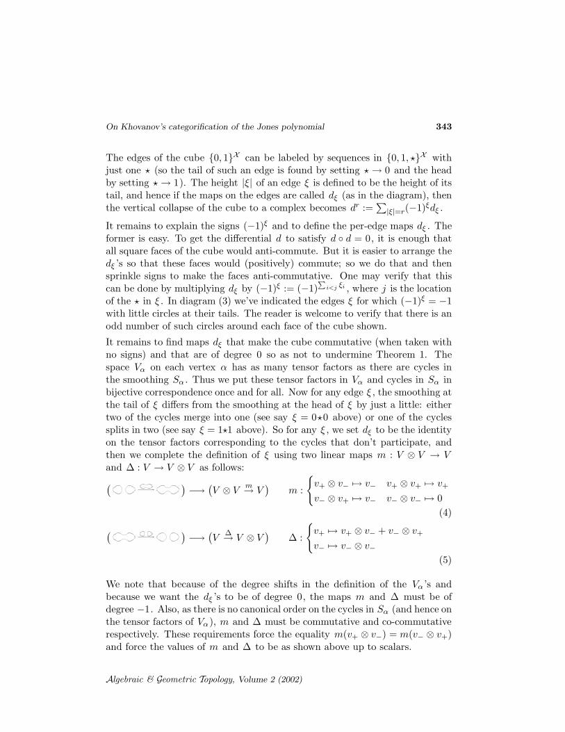
It remains to find maps dξ that make the cube commutative (when taken withno signs) and that are of degree 0 so as not to undermine Theorem 1. Thespace Vα on each vertex α has as many tensor factors as there are cycles inthe smoothing Sα . Thus we put these tensor factors in Vα and cycles in Sα inbijective correspondence once and for all. Now for any edge ξ , the smoothing atthe tail of ξ differs from the smoothing at the head of ξ by just a little: eithertwo of the cycles merge into one (see say ξ = 0⋆0 above) or one of the cyclessplits in two (see say ξ = 1⋆1 above). So for any ξ , we set dξ to be the identityon the tensor factors corresponding to the cycles that don’t participate, andthen we complete the definition of ξ using two linear maps m : V ⊗ V → Vand ∆ : V → V ⊗ V as follows:

( )

−→(

V ⊗ Vm→ V

)

m :

{

v+ ⊗ v− 7→ v− v+ ⊗ v+ 7→ v+

v− ⊗ v+ 7→ v− v− ⊗ v− 7→ 0

(4)

( )

−→(

V∆→ V ⊗ V

)

∆ :

{

v+ 7→ v+ ⊗ v− + v− ⊗ v+

v− 7→ v− ⊗ v−

(5)

We note that because of the degree shifts in the definition of the Vα ’s andbecause we want the dξ ’s to be of degree 0, the maps m and ∆ must be ofdegree −1. Also, as there is no canonical order on the cycles in Sα (and hence onthe tensor factors of Vα ), m and ∆ must be commutative and co-commutativerespectively. These requirements force the equality m(v+ ⊗ v−) = m(v− ⊗ v+)and force the values of m and ∆ to be as shown above up to scalars.


344 Dror Bar-Natan

Remark 3.4 It is worthwhile to note, though not strictly necessary to theunderstanding of this note, that the cube in diagram (3) is related to a certain(1 + 1)-dimensional topological quantum field theory (TQFT). Indeed, givenany (1 + 1)-dimensional TQFT one may assign vector spaces to the vertices of{0, 1}X and maps to the edges — on each vertex we have a union of cycles whichis a 1-manifold that gets mapped to a vector space via the TQFT, and on eachedge we can place the obvious 2-dimensional saddle-like cobordism between the1-manifolds on its ends, and then get a map between vector spaces using theTQFT. The cube in diagram (3) comes from this construction if one starts fromthe TQFT corresponding to the Frobenius algebra defined by V , m, ∆, theunit v+ and the co-unit ǫ ∈ V ⋆ defined by ǫ(v+) = 0, ǫ(v−) = 1. See morein [Kh1].

Exercise 3.5 Verify that the definitions given in this section agree with the“executive summary” (Section 1).

3.3 A notational digression

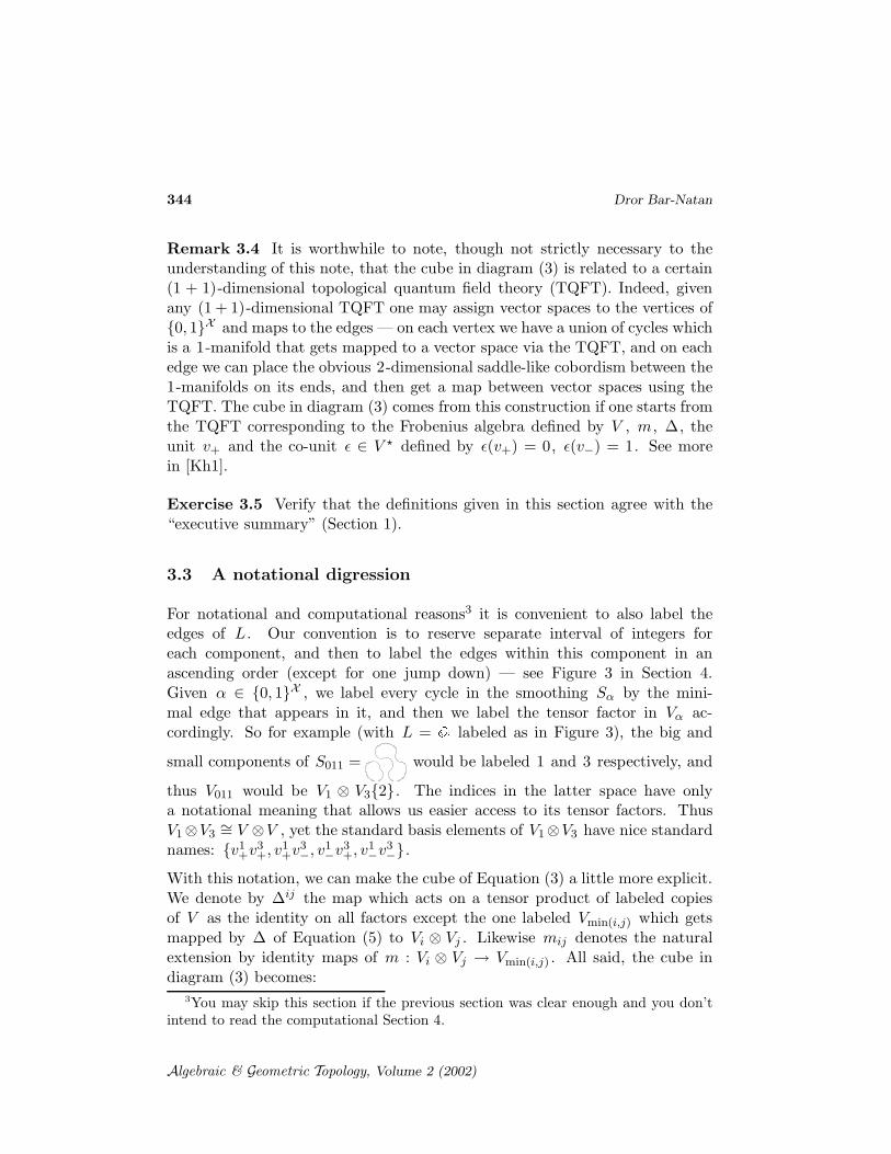
For notational and computational reasons3 it is convenient to also label theedges of L. Our convention is to reserve separate interval of integers foreach component, and then to label the edges within this component in anascending order (except for one jump down) — see Figure 3 in Section 4.Given α ∈ {0, 1}X , we label every cycle in the smoothing Sα by the mini-mal edge that appears in it, and then we label the tensor factor in Vα ac-cordingly. So for example (with L = & labeled as in Figure 3), the big and

small components of S011 = would be labeled 1 and 3 respectively, and

thus V011 would be V1 ⊗ V3{2}. The indices in the latter space have onlya notational meaning that allows us easier access to its tensor factors. ThusV1⊗V3

∼= V ⊗V , yet the standard basis elements of V1⊗V3 have nice standardnames: {v1

+v3+, v1

+v3−, v1

−v3+, v1

−v3−}.

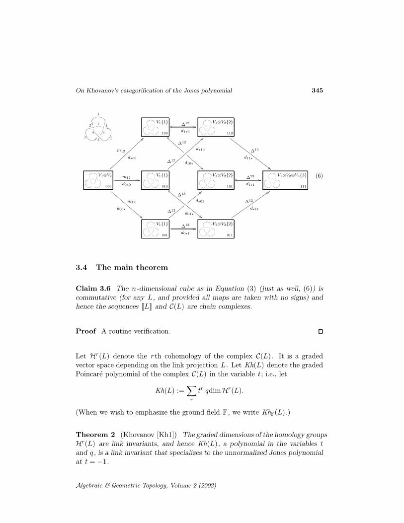
With this notation, we can make the cube of Equation (3) a little more explicit.We denote by ∆ij the map which acts on a tensor product of labeled copiesof V as the identity on all factors except the one labeled Vmin(i,j) which getsmapped by ∆ of Equation (5) to Vi ⊗ Vj . Likewise mij denotes the naturalextension by identity maps of m : Vi ⊗ Vj → Vmin(i,j) . All said, the cube indiagram (3) becomes:

3You may skip this section if the previous section was clear enough and you don’tintend to read the computational Section 4.



1

4

3

6

12

3

2

5

V1{1}

100

◦∆12

d1⋆0

//

◦

CCCC

CCCC

∆12

d10⋆

!!CCC

CCCC

C

V1⊗V2{2}

110

∆13

d11⋆

##FFFFFFFFFFFFFFFFFFF

V1⊗V2

000

m12

d⋆00

>>}}}}}}}}}}}}}}}}}

m12

d0⋆0

//

m12

d00⋆

!!DDDD

DDDD

DDDDD

DD

V1{1}

010

∆12

d⋆10

=={{{{{{{{{{{{{{{{{{

◦∆13

d01⋆""EE

EEEE

EEEE

EEEE

EE

V1⊗V2{2}

101

◦∆23

d1⋆1

//V1⊗V2⊗V3{3}

111

V1{1}

001

yyyyyyy∆12

d⋆01

<<yyyyyyy

∆13

d0⋆1

//V1⊗V3{2}

011

∆12

d⋆11

::vvvvvvvvvvvvvvvvv

(6)

3.4 The main theorem

Claim 3.6 The n-dimensional cube as in Equation (3) (just as well, (6)) iscommutative (for any L, and provided all maps are taken with no signs) andhence the sequences JLK and C(L) are chain complexes.

Proof A routine verification.

Let Hr(L) denote the rth cohomology of the complex C(L). It is a gradedvector space depending on the link projection L. Let Kh(L) denote the gradedPoincare polynomial of the complex C(L) in the variable t; i.e., let

Kh(L) :=∑

r

tr qdimHr(L).

(When we wish to emphasize the ground field F, we write KhF(L).)

Theorem 2 (Khovanov [Kh1]) The graded dimensions of the homology groupsHr(L) are link invariants, and hence Kh(L), a polynomial in the variables tand q , is a link invariant that specializes to the unnormalized Jones polynomialat t = −1.


346 Dror Bar-Natan

3.5 Proof of the main theorem

To prove Theorem 2, we need to study the behavior of JLK under the threeReidemeister moves4 (R1): ↔ , (R2): ↔ and (R3):

↔ . In the case of the Kauffman bracket/Jones polynomial,

this is done by reducing the Kauffman bracket of the “complicated side” of eachof these moves using the rules 〈0〉 = 〈1〉− q〈H〉 and 〈©L〉 = (q + q−1)〈L〉 andthen by canceling terms until the “easy side” is reached. (Example:

⟨ ⟩

=⟨ ⟩

− q⟨ ⟩

= (q + q−1)⟨ ⟩

− q⟨ ⟩

= q−1⟨ ⟩

). We do nearlythe same in the case of the Khovanov bracket. We first need to introduce a“cancellation principle” for chain complexes:

Lemma 3.7 Let C be a chain complex and let C′ ⊂ C be a sub chain complex.

• If C′ is acyclic (has no homology), then it can be “canceled”. That is, inthat case the homology H(C) of C is equal to the homology H(C/C′) ofC/C′ .

• Likewise, if C/C′ is acyclic then H(C) = H(C′).

Proof Both assertions follow easily from the long exact sequence

. . . −→ Hr(C′) −→ Hr(C) −→ Hr(C/C′) −→ Hr+1(C′) −→ . . .

associated with the short exact sequence 0 −→ C′ −→ C −→ C/C′ −→ 0.

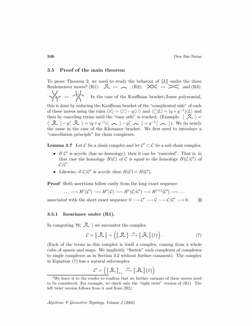
3.5.1 Invariance under (R1).

In computing H( ) we encounter the complex

C =q y

=(q y m

−→q y

{1})

. (7)

(Each of the terms in this complex is itself a complex, coming from a wholecube of spaces and maps. We implicitly “flatten” such complexes of complexesto single complexes as in Section 3.2 without further comment). The complexin Equation (7) has a natural subcomplex

C′ =(q y

v+

m−→

q y{1})

4We leave it to the reader to confirm that no further variants of these moves needto be considered. For example, we check only the “right twist” version of (R1). Theleft twist version follows from it and from (R2).



We need to pause to explain the notation. Recall that JLK is a direct sum overthe smoothings of L of tensor powers of V , with one tensor factor correspondingto each cycle in any given smoothing. Such tensor powers can be viewed asspaces of linear combinations of marked smoothings of L, where each cyclein any smoothing of L is marked by an element of V . For L = all

smoothings have one special cycle, the one appearing within the icon .

The subscript v+ inq y

v+means “the subspace of

q yin which the

special cycle is always marked v+”.

It is easy to check that C′ is indeed a subcomplex of C , and as v+ is a unit forthe product m (see (4)), C′ is acyclic. Thus by Lemma 3.7 we are reduced tostudying the quotient complex

C/C′ =(q y

/v+=0→ 0

)

where the subscript “/v+ = 0” means “mod out (within the tensor factor corre-sponding to the special cycle) by v+ = 0”. But V/(v+ = 0) is one dimensionaland generated by v− , and hence apart from a shift in degrees,

q y/v+=0

is isomorphic toq y

. The reader may verify that this shift precisely getscanceled by the shifts [−n−]{n+−2n−} in the definition of C(L) from JLK.

3.5.2 Invariance under (R2), first proof.

In computing H( ) we encounter the complex C of Figure 1. This com-plex has a subcomplex C′ (see Figure 1), which is clearly acyclic. The quotientcomplex C/C′ (see Figure 1) has a subcomplex C′′ (see Figure 1), and the quo-tient (C/C′)/C′′ (see Figure 1) is acyclic because modulo v+ = 0, the map∆ is an isomorphism. Hence using both parts of Lemma 3.7 we find thatH(C) = H(C/C′) = H(C′′). But up to shifts in degree and height, C′′ is justq y

. Again, these shifts get canceled by the shifts [−n−]{n+ − 2n−} inthe definition of C(L) from JLK.

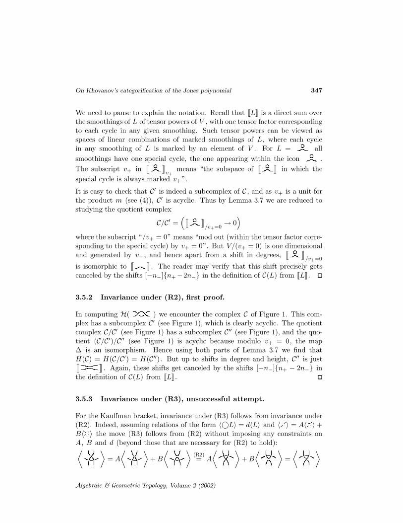
3.5.3 Invariance under (R3), unsuccessful attempt.

For the Kauffman bracket, invariance under (R3) follows from invariance under(R2). Indeed, assuming relations of the form 〈©L〉 = d〈L〉 and 〈0〉 = A〈1〉 +B〈H〉 the move (R3) follows from (R2) without imposing any constraints onA, B and d (beyond those that are necessary for (R2) to hold):⟨ ⟩

= A

⟨ ⟩

+ B

⟨ ⟩

(R2)= A

⟨ ⟩

+ B

⟨ ⟩

=

⟨ ⟩


348 Dror Bar-Natan

q y{1}

m //

C(start)

q y{2}

q y∆

OO

//q y

{1}

OO

⊃

q yv+{1} m //

C′

(acyclic)

q y{2}

0

OO

// 0

OO

q y/v+=0

{1} //

C/C′

(middle)

0

q y∆

OO

//q y

{1}

OO

⊃

0 //

C′′

(finish)

0

0

OO

//q y

{1}

OO

Figure 1: A picture-only proof of invariance under(R2). The (largely unnecessary) words are in themain text.

q y/v+=0

{1} //

(C/C′)/C′′

(acyclic)

0

q y∆

OO

// 0

OO

The case of the Khovanov bracket is unfortunately not as lucky. Invarianceunder (R2) does play a key role, but more is needed. Let us see how it works.

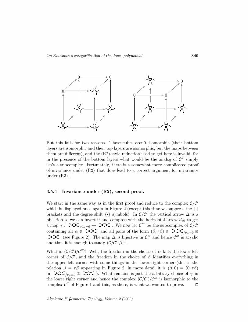
If we fully smooth the two sides of (R3), we get the following two cubes ofcomplexes (to save space we suppress the Khovanov bracket notation J·K andthe degree shifts {·}):

1

2 3

m //

OO OO∆@@��

//

OO

AA��

OO

//

//

@@��

AA��

1

32//

OO OO@@��∆ //

OO

mAA��

OO

//

//

@@��

AA��

(8)

The bottom layers of these two cubes correspond to the partial smoothings

and and are therefore isomorphic. The top layers correspond to

and and it is tempting to use (R2) on both to reduce to



0 //OO 0OO

0

=={{{{{{{{ //OO

=={{{{{{

OO

//

//

AA��

AA��

//

OO

0OO

0

=={{{{{{ //OO 0

=={{{{{{{{

OO

//

//

AA��

AA��

But this fails for two reasons. These cubes aren’t isomorphic (their bottomlayers are isomorphic and their top layers are isomorphic, but the maps betweenthem are different), and the (R2)-style reduction used to get here is invalid, forin the presence of the bottom layers what would be the analog of C′′ simplyisn’t a subcomplex. Fortunately, there is a somewhat more complicated proofof invariance under (R2) that does lead to a correct argument for invarianceunder (R3).

3.5.4 Invariance under (R2), second proof.

We start in the same way as in the first proof and reduce to the complex C/C′

which is displayed once again in Figure 2 (except this time we suppress the J·Kbrackets and the degree shift {·} symbols). In C/C′ the vertical arrow ∆ is abijection so we can invert it and compose with the horizontal arrow d⋆0 to geta map τ : /v+=0 → . We now let C′′′ be the subcomplex of C/C′

containing all α ∈ and all pairs of the form (β, τβ) ∈ /v+=0 ⊕

(see Figure 2). The map ∆ is bijective in C′′′ and hence C′′′ is acyclicand thus it is enough to study (C/C′)/C′′′ .

What is (C/C′)/C′′′? Well, the freedom in the choice of α kills the lower leftcorner of C/C′ , and the freedom in the choice of β identifies everything inthe upper left corner with some things in the lower right corner (this is therelation β = τβ appearing in Figure 2; in more detail it is (β, 0) = (0, τβ)in /v+=0 ⊕ ). What remains is just the arbitrary choice of γ inthe lower right corner and hence the complex (C/C′)/C′′′ is isomorphic to thecomplex C′′ of Figure 1 and this, as there, is what we wanted to prove.


350 Dror Bar-Natan

/v+=0// 0

∆

OO

d⋆0 //

OO

C/C′

⊃

β //

τ=d⋆0∆−1

))SSSSSSSSSSSSSS0

α

∆

OO

d⋆0 // τβ

OO

C′′′

Figure 2: A second proof of in-variance under (R2).

β //

β=τβ

))SSSSSSSSSSSSSS0

0

OO

// γ

OO

(C/C′)/C′′′

3.5.5 Invariance under (R3).

We can now turn back to the proof of invariance under (R3). Repeat thedefinitions of the acyclic subcomplexes C′ and C′′′ as above but within the toplayers of each of the cubes in Equation (8), and then mod out each cube byits C′ and C′′′ (without changing the homology, by Lemma 3.7). The resultingcubes are

β1 ∈ /v+=0//

OO

d1,⋆01

β1=τ1β1

&&LLLLL

0OO

0

::uuuuuuuu //OO γ1 ∈

=={{{{{{{

OO

d1,⋆10

//

//

::uuuuuuuuu

=={{{{{{

γ2 ∈ //

OO

d2,⋆01

0OO

0

=={{{{{{{{ //OO β2 ∈ /v+=0

::uuuuuuuuu

OO

d2,⋆10

τ2β2=β2

ffLLLLLL

//

//

=={{{{{{{

::uuuuuuuuu

Now these two complexes really are isomorphic, via the map Υ that keeps thebottom layers in place and “transposes” the top layers by mapping the pair(β1, γ1) to the pair (β2, γ2). The fact that Υ is an isomorphism on spaces levelis obvious. To see that Υ is an isomorphism of complexes we need to know thatit commutes with the edge maps, and only the vertical edges require a proof.We leave the (easy) proofs that τ1 ◦ d1,⋆01 = d2,⋆01 and d1,⋆10 = τ2 ◦ d2,⋆10 asexercises for our readers.



3.6 Some phenomenological conjectures

The following conjectures were formulated in parts by the author and by M. Kho-vanov and S. Garoufalidis based on computations using the program describedin the next section:

Conjecture 1 For any prime knot L there exists an even integer s = s(L)and a polynomial Kh′(L) in t±1 and q±1 with only non-negative coefficients sothat

KhQ(L) = qs−1(

1 + q2 + (1 + tq4)Kh′(L))

(9)

KhF2(L) = qs−1(1 + q2)

(

1 + (1 + tq2)Kh′(L))

. (10)

(F2 denotes the field of two elements.)

Conjecture 2 For prime alternating L the integer s(L) is equal to the signa-ture of L and the polynomial Kh′(L) contains only powers of tq2 .

We have computed KhQ(L) for all prime knots with up to 11 crossings andKhF2

(L) for all knots with up to 7 crossings and the results are in completeagreement with these two conjectures5.

We note that these conjectures imply that for alternating knots Kh′ (and henceKhQ and KhF2

) are determined by the Jones polynomial. As we shall see inthe next section, this is not true for non-alternating knots.

mr

-7 -6 -5 -4 -3 -2 -1 0 1 2 3

3 11 2-1 3 1-3 (4+1) 2-5 5 (3+1)-7 6 4-9 4 5-11 4 6-13 2 4-15 1 4-17 2-19 1

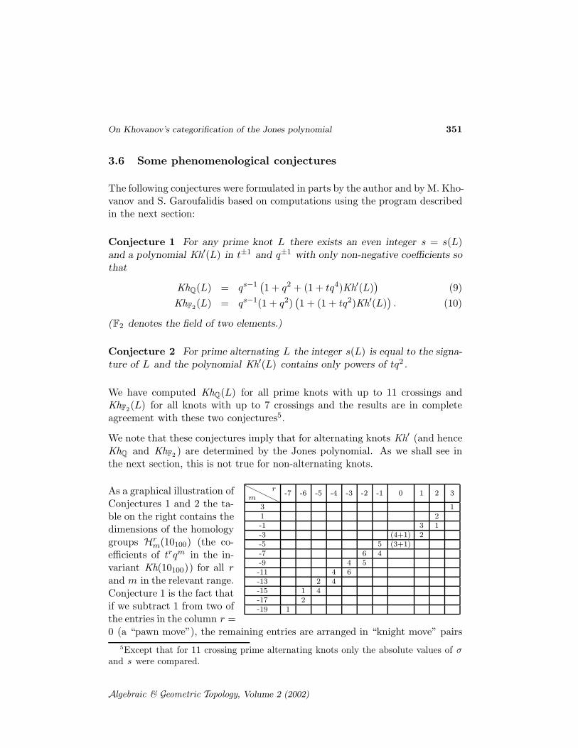
As a graphical illustration ofConjectures 1 and 2 the ta-ble on the right contains thedimensions of the homologygroups Hr

m(10100) (the co-efficients of trqm in the in-variant Kh(10100)) for all rand m in the relevant range.Conjecture 1 is the fact thatif we subtract 1 from two ofthe entries in the column r =0 (a “pawn move”), the remaining entries are arranged in “knight move” pairs

5Except that for 11 crossing prime alternating knots only the absolute values of σand s were compared.


352 Dror Bar-Natan

mr

-7 -6 -5 -4 -3 -2 -1 0 1 2 3

3 1/11 0/1 0/5 2/10 0/4-1 0/2 0/13 0/36 0/59 3/60 1/30 0/6-3 0/1 0/10 0/45 0/120 0/220 0/304 0/318 5/237 2/110 0/30 0/4-5 0/8 0/70 0/270 0/600 0/862 0/847 5/564 4/237 0/60 0/10 0/1-7 0/28 0/210 0/675 0/1200 0/1288 6/847 4/318 0/59 0/5-9 0/56 0/350 0/900 0/1200 4/862 5/304 0/36 0/1-11 0/70 0/350 0/675 4/600 6/220 0/13-13 0/56 0/210 2/270 4/120 0/2-15 0/28 1/70 4/45-17 0/8 2/10-19 1/1

Table 1: dimHrm(10100)/ dim Cr

m(10100) for all values of r and m for whichCr

m(10100) 6= ∅ .

of the forma

awith a > 0. Conjecture 2 is the fact that furthermore

all nontrivial entries in the table occur on just two diagonals that cross thecolumn r = 0 at m = σ ± 1 where σ = −4 is the signature of 10100 . Thus af-ter the fix at the r = 0 column, the two nontrivial diagonals are just shiftsof each other and are thus determined by a single list of entries (1 2 4 46 5 4 3 2 1, in our case). This list of entries is the list of coefficients ofKh′(10100) = u−7 + 2u−6 + 4u−5 + 4u−4 + 6u−3 + 5u−2 + 4u−1 + 3 + 2u + u2

(with u = tq4 ).

As an aside we note that typically dimHrm(L) is much smaller than dim Cr

m(L),as illustrated in Table 1. We don’t know why this is so.

A further phenomenological conjecture is presented in [Ga]. This paper’s webpage [1] will follow further phenomenological developments as they will be an-nounced.

4 And now in computer talk

In computer talk (Mathematica [Wo] dialect) we represent every link projectionby a list of edges numbered 1, . . . , n with increasing numbers as we go aroundeach component and by a list crossings presented as symbols Xijkl where i, . . . , lare the edges around that crossing, starting from the incoming lower thread andproceeding counterclockwise (see Figure 3).



i

l1 2

3

4 5

6

1

4

73

6

1

4

91112

3

k

j

2

5

2

3 5

6

8

10

12

Figure 3: The crossing Xijkl , the right handed trefoil knot X1524X5362X3146 and theMiller Institute knot (aka 62 ) X3,10,4,11X9,4,10,5X5,3,6,2X11,7,12,6X1,9,2,8X7,1,8,12 (we’veused a smaller font and underlining to separate the edge labeling from the vertexlabeling).

4.1 A demo run

We first start up Mathematica [Wo] and load our categorification package,Categorification‘ (available from [1]):

Mathematica 4.1 for Linux

Copyright 1988-2000 Wolfram Research, Inc.

-- Motif graphics initialized --

In[1]:= << Categorification‘

Loading Categorification‘...

Next, we type in the trefoil knot:

In[2]:= L = Link[X[1,5,2,4], X[5,3,6,2], X[3,1,4,6]];

Let us now view the edge 0⋆1 of the cube of smoothings of the trefoil knot (asseen in Section 3.3, this edge begins with a single cycle labeled 1 and ends withtwo cycles labeled 1 and 3):

In[3]:= {S[L, "001"], S[L, "0*1"], S[L, "011"]}

Out[3]= {c[1], c[1] -> c[1]*c[3], c[1]*c[3]}

Next, here’s a basis of the space V011 (again, compare with Section 3.3):


354 Dror Bar-Natan

In[4]:= V[L, "011"]

Out[4]= {vm[1]*vm[3], vm[3]*vp[1], vm[1]*vp[3], vp[1]*vp[3]}

And here’s a basis of the degree 2 elements of V111 (remember the shift indegrees in the definition of Vα !):

In[5]:= V[L, "111", 2]

Out[5]= {vm[2]*vm[3]*vp[1], vm[1]*vm[3]*vp[2], vm[1]*vm[2]*vp[3]}

The per-edge map dξ is a list of simple replacement rules, sometimes replacingthe tensor product of two basis vectors by a single basis vector, as in the caseof d00⋆ = m12 , and sometimes the opposite, as in the case of d0⋆1 = ∆13 :

In[6]:= d[L, "00*"]

Out[6]= {vp[1]*vp[2] -> vp[1], vm[2]*vp[1] -> vm[1], vm[1]*vp[2] -> vm[1],

vm[1]*vm[2] -> 0}

In[7]:= d[L, "0*1"]

Out[7]= {vp[1] -> vm[3]*vp[1] + vm[1]*vp[3], vm[1] -> vm[1]*vm[3]}

Here’s a simple example. Let us compute d1⋆1 applied to V101 :

In[8]:= V[L, "101"] /. d[L, "1*1"]

Out[8]= {vm[1]*vm[2]*vm[3], vm[2]*vm[3]*vp[1],

vm[1]*(vm[3]*vp[2] + vm[2]*vp[3]), vp[1]*(vm[3]*vp[2] + vm[2]*vp[3])}

And now a more complicated example. First, we compute the degree 0 part ofJ&K1 . Then we apply d1 to it, and then d2 to the result. The end result betterbe a list of zeros, or else we are in trouble! Notice that each basis vector inJ&K1,2 is tagged with a symbol of the form v[...] that indicates the componentof J&K1,2 to which it belongs.

In[9]:= chains = KhBracket[L, 1, 0]

Out[9]= {v[0, 0, 1]*vm[1], v[0, 1, 0]*vm[1], v[1, 0, 0]*vm[1]}



In[10]:= boundaries = d[L][chains]

Out[10]= {v[1, 0, 1]*vm[1]*vm[2] + v[0, 1, 1]*vm[1]*vm[3],

v[1, 1, 0]*vm[1]*vm[2] - v[0, 1, 1]*vm[1]*vm[3],

-(v[1, 0, 1]*vm[1]*vm[2]) - v[1, 1, 0]*vm[1]*vm[2]}

In[11]:= d[L][boundaries]

Out[11]= {0, 0, 0}

Because of degree shifts, the degree 3 part of C1(&) is equal to the degree 0part of J&K1 :

In[12]:= CC[L, 1, 3] == KhBracket[L, 1, 0]

Out[12]= True

It seems that H2(&) is one dimensional, and that the non trivial class in H2(&)lies in degree 5 (our program defaults to computations over the rational num-bers if no other modulus is specified):

In[13]:= qBetti[L, 2]

Out[13]= q^5

Here’s Khovanov’s invariant of the right handed trefoil along if its evaluationat t = −1, the unnormalized Jones polynomial J(&):

In[14]:= kh1 = Kh[L]

Out[14]= q + q^3 + q^5*t^2 + q^9*t^3

In[15]:= kh1 /. t -> -1

Out[15]= q + q^3 + q^5 - q^9

We can also compute KhF2(&) and use it to compute J(&) again (we leave it

to the reader to verify Conjecture 1 in the case of L = &):

In[16]:= kh2 = Kh[L, Modulus -> 2]


356 Dror Bar-Natan

Out[16]= q + q^3 + q^5*t^2 + q^7*t^2 + q^7*t^3 + q^9*t^3

In[17]:= kh2 /. t -> -1

Out[17]= q + q^3 + q^5 - q^9

1

2

4

5

8 9

20

36

7

101112

13

14

1517

18

19

16

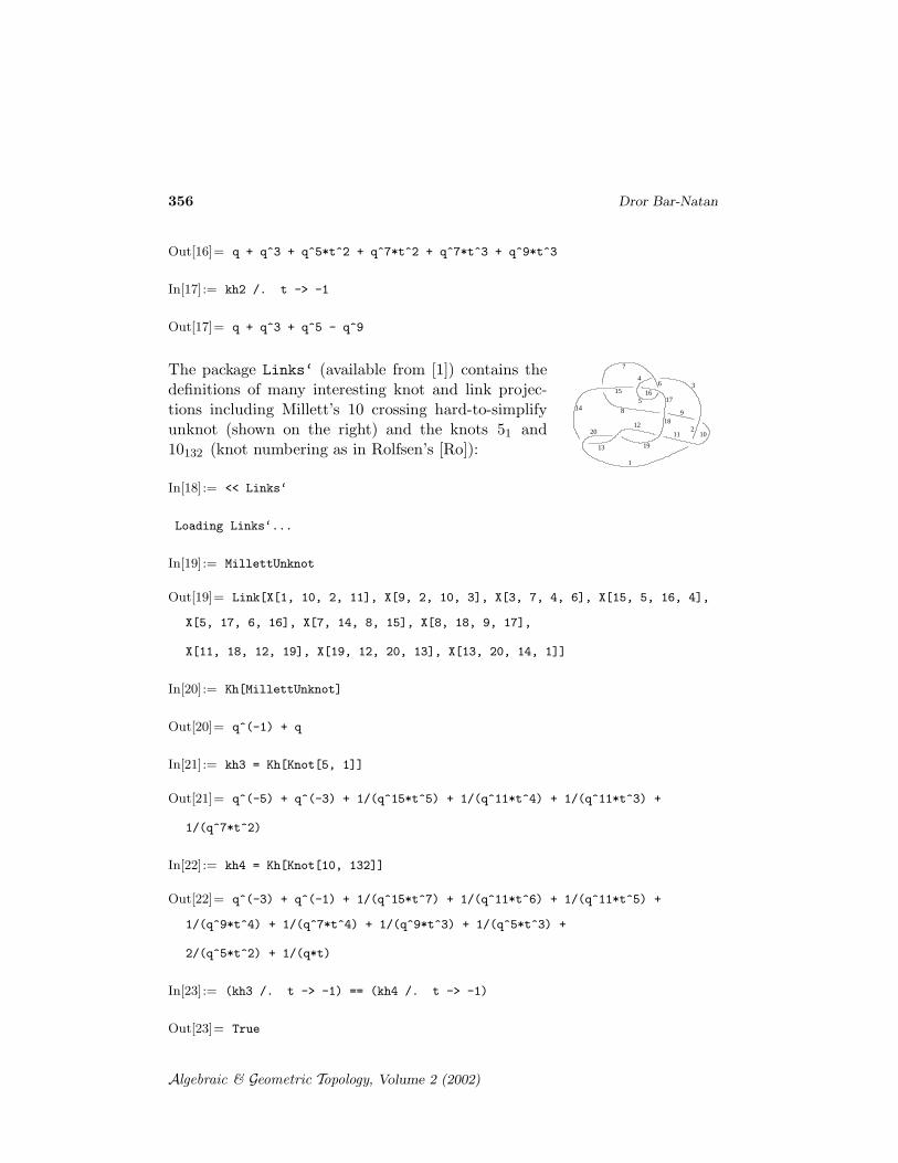
The package Links‘ (available from [1]) contains thedefinitions of many interesting knot and link projec-tions including Millett’s 10 crossing hard-to-simplifyunknot (shown on the right) and the knots 51 and10132 (knot numbering as in Rolfsen’s [Ro]):

In[18]:= << Links‘

Loading Links‘...

In[19]:= MillettUnknot

Out[19]= Link[X[1, 10, 2, 11], X[9, 2, 10, 3], X[3, 7, 4, 6], X[15, 5, 16, 4],

X[5, 17, 6, 16], X[7, 14, 8, 15], X[8, 18, 9, 17],

X[11, 18, 12, 19], X[19, 12, 20, 13], X[13, 20, 14, 1]]

In[20]:= Kh[MillettUnknot]

Out[20]= q^(-1) + q

In[21]:= kh3 = Kh[Knot[5, 1]]

Out[21]= q^(-5) + q^(-3) + 1/(q^15*t^5) + 1/(q^11*t^4) + 1/(q^11*t^3) +

1/(q^7*t^2)

In[22]:= kh4 = Kh[Knot[10, 132]]

Out[22]= q^(-3) + q^(-1) + 1/(q^15*t^7) + 1/(q^11*t^6) + 1/(q^11*t^5) +

1/(q^9*t^4) + 1/(q^7*t^4) + 1/(q^9*t^3) + 1/(q^5*t^3) +

2/(q^5*t^2) + 1/(q*t)

In[23]:= (kh3 /. t -> -1) == (kh4 /. t -> -1)

Out[23]= True



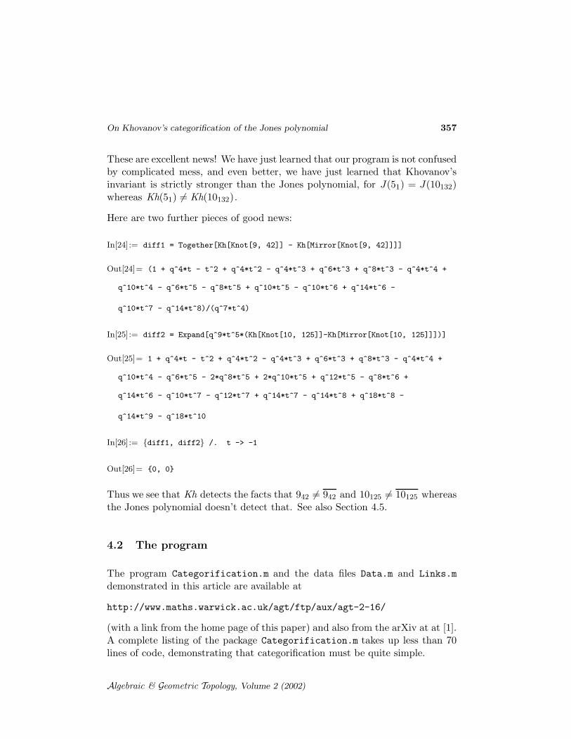
These are excellent news! We have just learned that our program is not confusedby complicated mess, and even better, we have just learned that Khovanov’sinvariant is strictly stronger than the Jones polynomial, for J(51) = J(10132)whereas Kh(51) 6= Kh(10132).

Here are two further pieces of good news:

In[24]:= diff1 = Together[Kh[Knot[9, 42]] - Kh[Mirror[Knot[9, 42]]]]

Out[24]= (1 + q^4*t - t^2 + q^4*t^2 - q^4*t^3 + q^6*t^3 + q^8*t^3 - q^4*t^4 +

q^10*t^4 - q^6*t^5 - q^8*t^5 + q^10*t^5 - q^10*t^6 + q^14*t^6 -

q^10*t^7 - q^14*t^8)/(q^7*t^4)

In[25]:= diff2 = Expand[q^9*t^5*(Kh[Knot[10, 125]]-Kh[Mirror[Knot[10, 125]]])]

Out[25]= 1 + q^4*t - t^2 + q^4*t^2 - q^4*t^3 + q^6*t^3 + q^8*t^3 - q^4*t^4 +

q^10*t^4 - q^6*t^5 - 2*q^8*t^5 + 2*q^10*t^5 + q^12*t^5 - q^8*t^6 +

q^14*t^6 - q^10*t^7 - q^12*t^7 + q^14*t^7 - q^14*t^8 + q^18*t^8 -

q^14*t^9 - q^18*t^10

In[26]:= {diff1, diff2} /. t -> -1

Out[26]= {0, 0}

Thus we see that Kh detects the facts that 942 6= 942 and 10125 6= 10125 whereasthe Jones polynomial doesn’t detect that. See also Section 4.5.

4.2 The program

The program Categorification.m and the data files Data.m and Links.m

demonstrated in this article are available at

http://www.maths.warwick.ac.uk/agt/ftp/aux/agt-2-16/

(with a link from the home page of this paper) and also from the arXiv at at [1].A complete listing of the package Categorification.m takes up less than 70lines of code, demonstrating that categorification must be quite simple.


358 Dror Bar-Natan

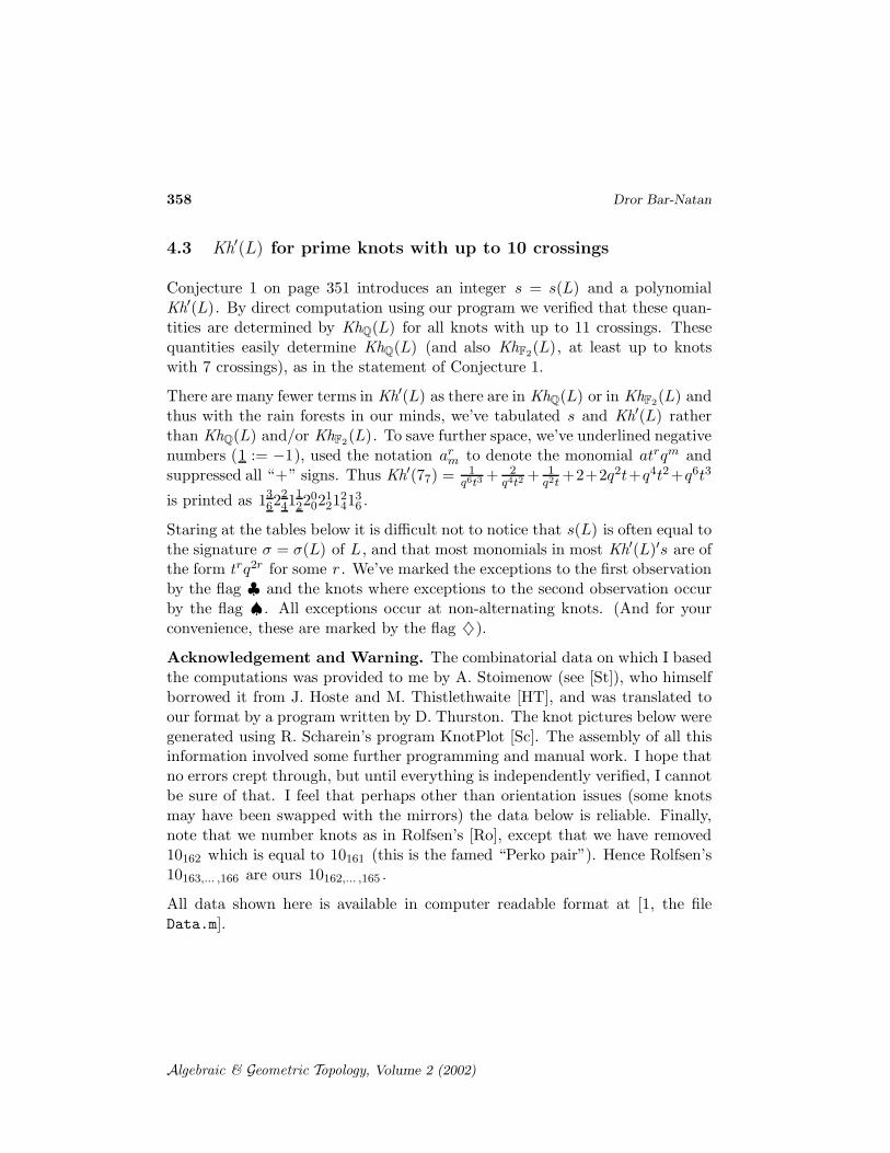
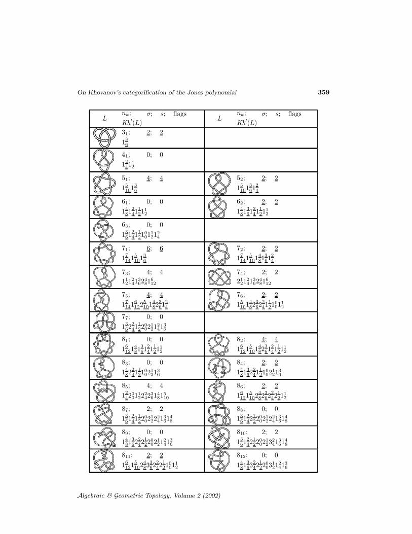
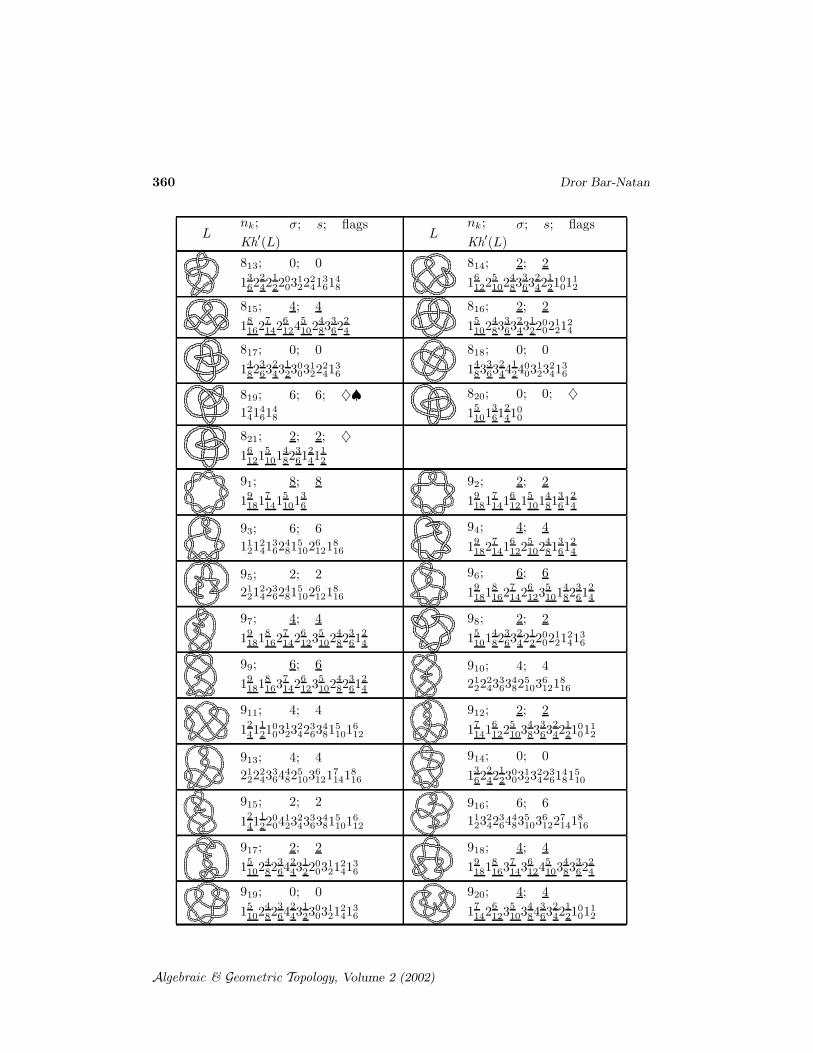
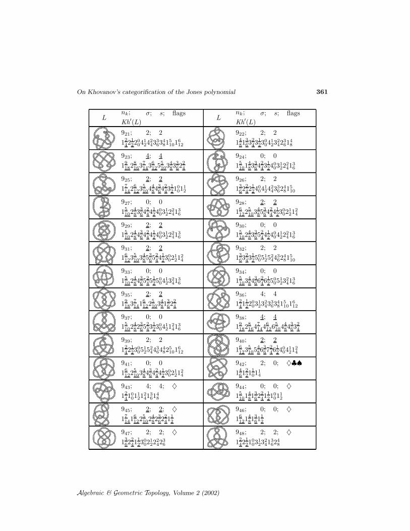
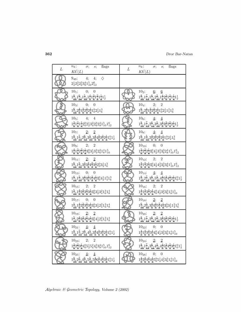
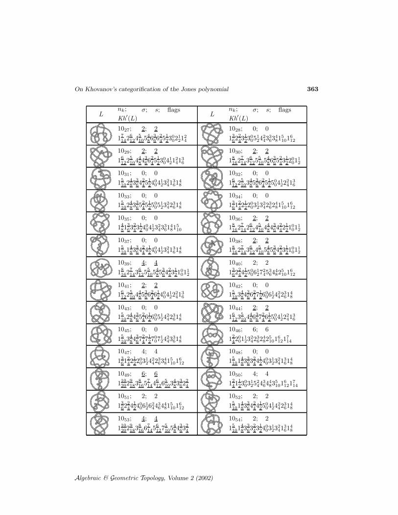
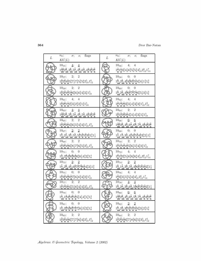
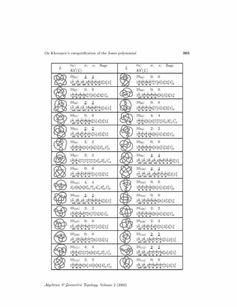
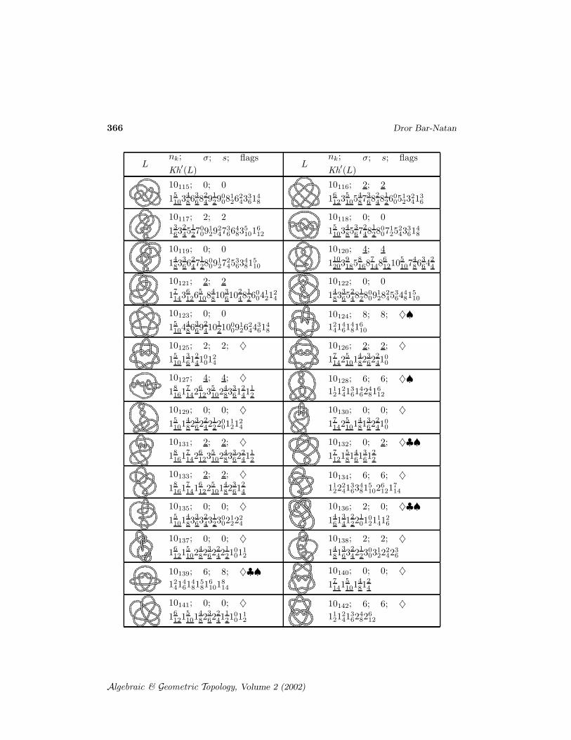
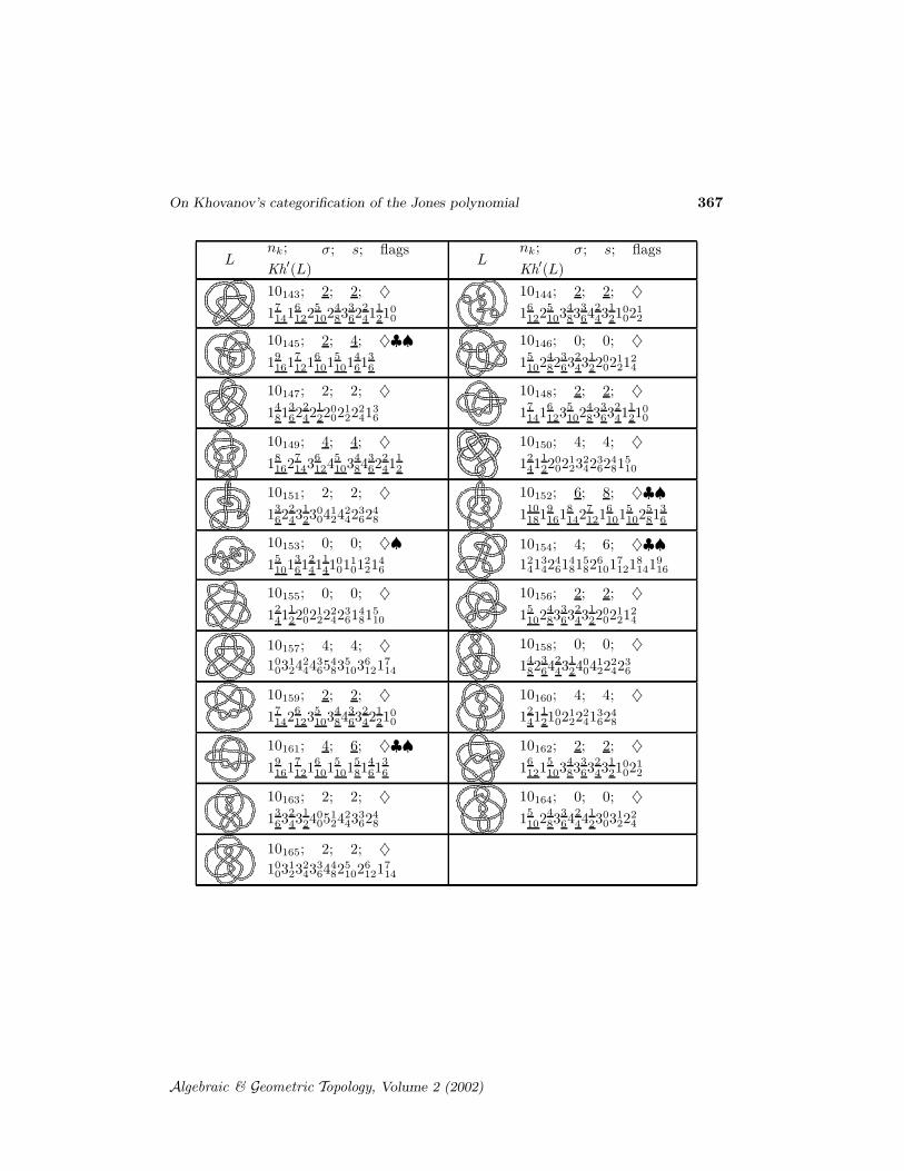
4.3 Kh′(L) for prime knots with up to 10 crossings

Conjecture 1 on page 351 introduces an integer s = s(L) and a polynomialKh′(L). By direct computation using our program we verified that these quan-tities are determined by KhQ(L) for all knots with up to 11 crossings. Thesequantities easily determine KhQ(L) (and also KhF2

(L), at least up to knotswith 7 crossings), as in the statement of Conjecture 1.

There are many fewer terms in Kh′(L) as there are in KhQ(L) or in KhF2(L) and

thus with the rain forests in our minds, we’ve tabulated s and Kh′(L) ratherthan KhQ(L) and/or KhF2

(L). To save further space, we’ve underlined negativenumbers (1 := −1), used the notation ar

m to denote the monomial atrqm andsuppressed all “+” signs. Thus Kh′(77) = 1

q6t3+ 2

q4t2+ 1

q2t+2+2q2t+q4t2+q6t3

is printed as 1362

241

122

002

121

241

36 .

Staring at the tables below it is difficult not to notice that s(L) is often equal tothe signature σ = σ(L) of L, and that most monomials in most Kh′(L)′s are ofthe form trq2r for some r . We’ve marked the exceptions to the first observationby the flag ♣ and the knots where exceptions to the second observation occurby the flag ♠. All exceptions occur at non-alternating knots. (And for yourconvenience, these are marked by the flag ♦).

Acknowledgement and Warning. The combinatorial data on which I basedthe computations was provided to me by A. Stoimenow (see [St]), who himselfborrowed it from J. Hoste and M. Thistlethwaite [HT], and was translated toour format by a program written by D. Thurston. The knot pictures below weregenerated using R. Scharein’s program KnotPlot [Sc]. The assembly of all thisinformation involved some further programming and manual work. I hope thatno errors crept through, but until everything is independently verified, I cannotbe sure of that. I feel that perhaps other than orientation issues (some knotsmay have been swapped with the mirrors) the data below is reliable. Finally,note that we number knots as in Rolfsen’s [Ro], except that we have removed10162 which is equal to 10161 (this is the famed “Perko pair”). Hence Rolfsen’s10163,... ,166 are ours 10162,... ,165 .

All data shown here is available in computer readable format at [1, the fileData.m].



Lnk; σ; s; flags

Kh′(L)L

nk; σ; s; flags

Kh′(L)

31; 2; 2

13

6

41; 0; 0

12

4112

51; 4; 4

15

1013

6

52; 2; 2

15

1013

612

4

61; 0; 0

14

812

411

2112

62; 2; 2

14

813

612

411

2112

63; 0; 0

13

612

411

21001

121

24

71; 6; 6

17

1415

1013

6

72; 2; 2

17

1415

1014

813

612

4

73; 4; 4

1121

241

362

481

612

74; 2; 2

2121

241

362

481

612

75; 4; 4

17

1416

1225

1014

823

612

4

76; 2; 2

15

1014

823

622

411

21001

12

77; 0; 0

13

622

411

22002

121

241

36

81; 0; 0

16

1214

813

612

411

2112

82; 4; 4

16

1215

1014

823

612

411

2112

83; 0; 0

14

822

411

21002

121

36

84; 2; 2

14

813

622

411

21002

121

36

85; 4; 4

12

42001

122

242

361

481

510

86; 2; 2

16

1215

1024

823

622

421

2112

87; 2; 2

13

612

411

22002

122

241

361

48

88; 0; 0

13

612

421

22002

122

241

361

48

89; 0; 0

14

813

622

421

22002

121

241

36

810; 2; 2

13

612

421

22002

123

241

361

48

811; 2; 2

16

1215

1024

833

622

421

21001

12

812; 0; 0

14

813

632

421

22003

121

241

36


360 Dror Bar-Natan

Lnk; σ; s; flags

Kh′(L)L

nk; σ; s; flags

Kh′(L)

813; 0; 0

13

622

421

22003

122

241

361

48

814; 2; 2

16

1225

1024

833

632

421

21001

12

815; 4; 4

18

1627

1426

1245

1024

833

622

4

816; 2; 2

15

1024

833

632

431

22002

121

24

817; 0; 0

14

823

632

431

23003

122

241

36

818; 0; 0

14

833

632

441

24003

123

241

36

819; 6; 6; ♦♠

1241

461

48

820; 0; 0; ♦

15

1013

612

4100

821; 2; 2; ♦

16

1215

1014

823

612

411

2

91; 8; 8

19

1817

1415

1013

6

92; 2; 2

19

1817

1416

1215

1014

813

612

4

93; 6; 6

1121

241

362

481

5102

6121

816

94; 4; 4

19

1827

1416

1225

1024

813

612

4

95; 2; 2

2121

242

362

481

5102

6121

816

96; 6; 6

19

1818

1627

1426

1235

1014

823

612

4

97; 4; 4

19

1818

1627

1426

1235

1024

823

612

4

98; 2; 2

15

1014

823

632

421

22002

121

241

36

99; 6; 6

19

1818

1637

1426

1235

1024

823

612

4

910; 4; 4

2122

243

363

482

5103

6121

816

911; 4; 4

12

411

21003

123

242

363

481

5101

612

912; 2; 2

17

1416

1225

1034

833

632

421

21001

12

913; 4; 4

2122

243

364

482

5103

6121

7141

816

914; 0; 0

13

622

421

23003

123

242

361

481

510

915; 2; 2

12

411

22004

123

243

363

481

5101

612

916; 6; 6

1123

242

364

483

5103

6122

7141

816

917; 2; 2

15

1024

823

642

431

22003

121

241

36

918; 4; 4

19

1818

1637

1436

1245

1034

833

622

4

919; 0; 0

15

1024

823

642

431

23003

121

241

36

920; 4; 4

17

1426

1235

1034

843

632

421

21001

12



Lnk; σ; s; flags

Kh′(L)L

nk; σ; s; flags

Kh′(L)

921; 2; 2

12

421

22004

124

243

363

481

5101

612

922; 2; 2

14

813

632

431

23004

123

242

361

48

923; 4; 4

19

1828

1637

1436

1255

1034

833

622

4

924; 0; 0

15

1014

833

642

431

24003

122

241

36

925; 2; 2

17

1426

1235

1044

843

642

431

21001

12

926; 2; 2

13

622

421

24004

124

243

362

481

510

927; 0; 0

15

1024

833

642

441

24003

122

241

36

928; 2; 2

16

1225

1034

853

642

441

23002

121

24

929; 2; 2

15

1024

843

642

441

24003

122

241

36

930; 0; 0

15

1024

833

652

441

24004

122

241

36

931; 2; 2

16

1235

1034

853

652

441

23002

121

24

932; 2; 2

13

632

431

25005

125

244

362

481

510

933; 0; 0

15

1024

843

652

451

25004

123

241

36

934; 0; 0

15

1034

843

662

461

25005

123

241

36

935; 2; 2

19

1837

1416

1225

1034

813

622

4

936; 4; 4

12

411

22003

123

243

363

481

5101

612

937; 0; 0

15

1024

823

652

431

23004

121

241

36

938; 4; 4

19

1828

1647

1446

1265

1044

843

632

4

939; 2; 2

12

421

23005

125

244

364

482

5101

612

940; 2; 2

16

1235

1054

863

672

461

24004

121

24

941; 0; 0

16

1225

1034

843

642

441

23002

121

24

942; 2; 0; ♦♣♠

14

612

211

0114

943; 4; 4; ♦

12

41001

121

241

361

48

944; 0; 0; ♦

15

1014

813

622

411

21001

12

945; 2; 2; ♦

17

1416

1225

1024

823

622

411

2

946; 0; 0; ♦

16

1214

813

611

2

947; 2; 2; ♦

13

622

411

23002

122

242

36

948; 2; 2; ♦

12

421

21003

123

241

362

48


362 Dror Bar-Natan

Lnk; σ; s; flags

Kh′(L)L

nk; σ; s; flags

Kh′(L)

949; 4; 4; ♦

2122

242

363

481

5102

612

101; 0; 0

18

1616

1215

1014

813

612

411

2112

102; 6; 6

18

1617

1416

1225

1014

823

612

411

2112

103; 0; 0

16

1224

813

622

421

21002

121

36

104; 2; 2

16

1224

813

622

421

21002

121

241

36

105; 4; 4

13

612

411

22002

123

242

362

481

5101

612

106; 4; 4

18

1617

1426

1235

1034

833

622

421

2112

107; 2; 2

18

1617

1426

1235

1034

843

632

421

21001

12

108; 4; 4

16

1215

1024

823

622

421

21002

121

36

109; 2; 2

14

813

622

421

23003

123

242

361

481

510

1010; 0; 0

13

622

421

23004

123

243

362

481

5101

612

1011; 2; 2

16

1215

1034

833

642

431

22003

121

36

1012; 2; 2

13

612

421

23004

124

243

363

481

5101

612

1013; 0; 0

16

1215

1034

833

652

441

23004

121

241

36

1014; 4; 4

18

1627

1436

1255

1044

853

642

421

21001

12

1015; 2; 2

15

1014

823

632

431

23003

123

241

361

48

1016; 2; 2

14

813

632

421

24004

123

243

361

481

510

1017; 0; 0

15

1014

823

632

431

23003

122

241

361

48

1018; 2; 2

16

1225

1034

843

652

441

23003

121

241

36

1019; 2; 2

15

1024

833

642

441

23004

122

241

361

48

1020; 2; 2

18

1617

1426

1225

1034

833

622

421

2112

1021; 4; 4

18

1617

1426

1245

1034

843

632

421

21001

12

1022; 0; 0

14

813

632

431

24004

123

243

361

481

510

1023; 2; 2

13

622

431

24005

125

244

363

481

5101

612

1024; 2; 2

18

1617

1436

1245

1044

853

642

431

21001

12

1025; 4; 4

18

1627

1446

1255

1054

863

642

431

21001

12

1026; 0; 0

14

823

642

441

25005

124

243

361

481

510



Lnk; σ; s; flags

Kh′(L)L

nk; σ; s; flags

Kh′(L)

1027; 2; 2

17

1426

1245

1054

863

662

451

23002

121

24

1028; 0; 0

13

622

431

23005

124

243

363

481

5101

612

1029; 2; 2

16

1225

1044

843

662

451

23004

121

241

36

1030; 2; 2

18

1627

1436

1255

1054

863

652

431

22001

12

1031; 0; 0

15

1024

833

642

451

24004

123

241

361

48

1032; 0; 0

16

1225

1034

853

662

451

25004

122

241

36

1033; 0; 0

15

1024

833

652

451

25005

123

242

361

48

1034; 0; 0

13

612

421

22003

123

242

362

481

5101

612

1035; 0; 0

14

813

632

431

24004

123

243

361

481

510

1036; 2; 2

18

1627

1426

1245

1044

843

642

421

21001

12

1037; 0; 0

15

1014

833

642

441

24004

123

241

361

48

1038; 2; 2

18

1627

1436

1245

1054

853

642

431

21001

12

1039; 4; 4

18

1627

1436

1255

1054

853

642

431

21001

12

1040; 2; 2

13

622

441

25006

127

245

364

482

5101

612

1041; 2; 2

16

1225

1044

853

662

461

24004

122

241

36

1042; 0; 0

15

1034

843

662

471

26006

124

242

361

48

1043; 0; 0

15

1024

843

652

461

26005

124

242

361

48

1044; 2; 2

16

1235

1044

863

672

461

25004

122

241

36

1045; 0; 0

15

1034

843

672

471

27007

124

243

361

48

1046; 6; 6

12

42001

123

242

362

482

5101

6121

714

1047; 4; 4

13

612

421

22003

124

242

363

481

5101

612

1048; 0; 0

15

1014

833

632

441

24003

123

241

361

48

1049; 6; 6

110

2029

1838

1657

1446

1265

1034

833

622

4

1050; 4; 4

12

411

23003

125

244

364

483

5101

6121

714

1051; 2; 2

13

622

441

24006

126

244

364

481

5101

612

1052; 2; 2

15

1014

833

642

441

25004

124

242

361

48

1053; 4; 4

110

2029

1838

1667

1456

1275

1054

843

632

4

1054; 2; 2

15

1014

833

632

431

24003

123

241

361

48


364 Dror Bar-Natan

Lnk; σ; s; flags

Kh′(L)L

nk; σ; s; flags

Kh′(L)

1055; 4; 4

110

2029

1838

1657

1446

1265

1044

833

622

4

1056; 4; 4

12

411

23004

126

245

365

484

5102

6121

714

1057; 2; 2

13

622

441

25007

127

245

365

482

5101

612

1058; 0; 0

16

1225

1044

843

662

451

24004

121

241

36

1059; 2; 2

14

823

642

451

26006

126

244

362

481

510

1060; 0; 0

16

1225

1044

863

672

471

26005

123

241

36

1061; 4; 4

14

832

411

22003

122

242

361

481

510

1062; 4; 4

13

612

421

23003

124

243

363

481

5101

612

1063; 4; 4

110

2029

1828

1657

1446

1255

1044

833

622

4

1064; 2; 2

14

813

632

431

24004

124

243

361

481

510

1065; 2; 2

13

622

431

24006

125

244

364

481

5101

612

1066; 6; 6

110

2039

1848

1667

1466

1275

1044

843

622

4

1067; 2; 2

18

1627

1436

1255

1054

853

652

431

21001

12

1068; 0; 0

17

1416

1235

1044

843

652

441

23002

121

24

1069; 2; 2

13

632

441

26008

127

246

365

482

5101

612

1070; 2; 2

14

813

642

441

25006

125

244

362

481

510

1071; 0; 0

15

1024

843

662

461

26006

124

242

361

48

1072; 4; 4

12

411

23005

126

246

366

484

5103

6121

714

1073; 2; 2

17

1426

1245

1064

873

672

461

24003

121

24

1074; 2; 2

18

1617

1436

1255

1044

863

652

431

22001

12

1075; 0; 0

14

833

642

461

27006

126

244

362

481

510

1076; 4; 4

12

43003

125

245

364

484

5102

6121

714

1077; 2; 2

13

612

431

24005

126

244

364

482

5101

612

1078; 4; 4

18

1627

1436

1265

1054

863

652

431

22001

12

1079; 0; 0

15

1014

843

642

451

25004

124

241

361

48

1080; 6; 6

110

2029

1848

1667

1456

1275

1044

843

622

4

1081; 0; 0

15

1024

853

662

471

27006

125

242

361

48

1082; 2; 2

16

1225

1034

853

652

451

24003

122

241

36

1083; 2; 2

13

632

441

26007

127

246

364

482

5101

612

1084; 2; 2

13

622

441

26007

128

246

365

483

5101

612



Lnk; σ; s; flags

Kh′(L)L

nk; σ; s; flags

Kh′(L)

1085; 4; 4

17

1426

1235

1044

853

642

441

22002

121

24

1086; 0; 0

14

833

652

461

27007

126

244

362

481

510

1087; 0; 0

14

823

642

461

26007

126

244

363

481

510

1088; 0; 0

15

1034

853

682

481

28008

125

243

361

48

1089; 2; 2

17

1426

1255

1074

883

692

471

25004

121

24

1090; 0; 0

14

823

652

451

26007

125

244

362

481

510

1091; 0; 0

15

1024

843

652

461

26005

124

242

361

48

1092; 4; 4

12

421

24006

128

247

367

485

5103

6121

714

1093; 2; 2

15

1024

843

652

451

25005

123

242

361

48

1094; 2; 2

14

823

642

441

26006

125

244

362

481

510

1095; 2; 2

13

632

451

26008

128

246

365

482

5101

612

1096; 0; 0

14

833

662

461

28008

126

245

362

481

510

1097; 2; 2

12

421

24007

127

247

367

484

5103

6121

714

1098; 4; 4

18

1627

1456

1265

1064

883

652

441

22001

12

1099; 0; 0

15

1024

853

652

471

27005

125

242

361

48

10100; 4; 4

17

1426

1245

1044

863

652

441

23002

121

24

10101; 4; 4

3124

246

368

486

5107

6124

7143

8161

918

10102; 0; 0

14

823

642

451

26006

125

244

362

481

510

10103; 2; 2

17

1426

1245

1054

873

662

451

24002

121

24

10104; 0; 0

15

1024

843

662

461

26006

124

242

361

48

10105; 2; 2

14

823

652

461

27008

127

245

363

481

510

10106; 2; 2

14

823

642

451

26006

126

244

362

481

510

10107; 0; 0

15

1034

853

672

481

27007

125

242

361

48

10108; 2; 2

15

1024

833

652

441

25005

123

242

361

48

10109; 0; 0

15

1024

853

662

471

27006

125

242

361

48

10110; 2; 2

16

1225

1054

863

672

471

25005

122

241

36

10111; 4; 4

12

421

24005

127

246

366

484

5102

6121

714

10112; 2; 2

16

1235

1044

873

672

471

26004

123

241

36

10113; 2; 2

13

632

451

28009

12102

48366

484

5101

612

10114; 0; 0

16

1235

1044

873

682

471

27005

123

241

36


366 Dror Bar-Natan

Lnk; σ; s; flags

Kh′(L)L

nk; σ; s; flags

Kh′(L)

10115; 0; 0

15

1034

863

682

491

29008

126

243

361

48

10116; 2; 2

16

1235

1054

873

682

481

26005

123

241

36

10117; 2; 2

13

632

451

27009

129

247

366

483

5101

612

10118; 0; 0

15

1034

853

672

481

28007

125

243

361

48

10119; 0; 0

14

833

662

471

28009

127

245

363

481

510

10120; 4; 4

110

2039

1858

1687

1486

12105

1074

863

642

4

10121; 2; 2

17

1436

1265

1084

8103

6102

481

26004

121

24

10122; 0; 0

14

833

652

481

28009

128

245

364

481

510

10123; 0; 0

15

1044

863

692

4101

210009

126

244

361

48

10124; 8; 8; ♦♠

1241

461

481

610

10125; 2; 2; ♦

15

1013

612

41001

24

10126; 2; 2; ♦

17

1425

1014

823

622

4100

10127; 4; 4; ♦

18

1617

1426

1235

1024

833

612

411

2

10128; 6; 6; ♦♠

1121

241

361

462

481

612

10129; 0; 0; ♦

15

1014

823

622

421

22001

121

24

10130; 0; 0; ♦

17

1425

1014

813

622

4100

10131; 2; 2; ♦

18

1617

1426

1235

1024

833

622

411

2

10132; 0; 2; ♦♣♠

17

1215

814

613

612

2

10133; 2; 2; ♦

18

1617

1416

1225

1014

823

612

4

10134; 6; 6; ♦

1122

241

363

481

5102

6121

714

10135; 0; 0; ♦

15

1014

833

632

431

23002

122

24

10136; 2; 0; ♦♣♠

14

613

412

221

01021

141

26

10137; 0; 0; ♦

16

1215

1024

823

622

421

21001

12

10138; 2; 2; ♦

14

813

632

421

23003

122

242

36

10139; 6; 8; ♦♣♠

1241

461

481

581

6101

814

10140; 0; 0; ♦

17

1415

1014

812

4

10141; 0; 0; ♦

16

1215

1014

823

622

411

21001

12

10142; 6; 6; ♦

1121

241

362

482

612



Lnk; σ; s; flags

Kh′(L)L

nk; σ; s; flags

Kh′(L)

10143; 2; 2; ♦

17

1416

1225

1024

833

622

411

2100

10144; 2; 2; ♦

16

1225

1034

833

642

431

21002

12

10145; 2; 4; ♦♣♠

19

1617

1216

1015

1014

613

6

10146; 0; 0; ♦

15

1024

823

632

431

22002

121

24

10147; 2; 2; ♦

14

813

622

421

22002

122

241

36

10148; 2; 2; ♦

17

1416

1235

1024

833

632

411

2100

10149; 4; 4; ♦

18

1627

1436

1245

1034

843

622

411

2

10150; 4; 4; ♦

12

411

22002

123

242

362

481

510

10151; 2; 2; ♦

13

622

431

23004

124

242

362

48

10152; 6; 8; ♦♣♠

110

1819

1618

1427

1216

1015

1025

813

6

10153; 0; 0; ♦♠

15

1013

612

411

41001

101

221

46

10154; 4; 6; ♦♣♠

1241

342

461

481

582

6101

7121

8141

916

10155; 0; 0; ♦

12

411

22002

122

242

361

481

510

10156; 2; 2; ♦

15

1024

833

632

431

22002

121

24

10157; 4; 4; ♦

1003

124

244

365

483

5103

6121

714

10158; 0; 0; ♦

14

823

642

431

24004

122

242

36

10159; 2; 2; ♦

17

1426

1235

1034

843

632

421

2100

10160; 4; 4; ♦

12

411

21002

122

241

362

48

10161; 4; 6; ♦♣♠

19

1617

1216

1015

1015

814

613

6

10162; 2; 2; ♦

16

1215

1034

833

632

431

21002

12

10163; 2; 2; ♦

13

632

431

24005

124

243

362

48

10164; 0; 0; ♦

15

1024

833

642

441

23003

122

24

10165; 2; 2; ♦

1003

123

243

364

482

5102

6121

714


368 Dror Bar-Natan

4.4 Kh′(L) for prime knots with 11 crossings

This data is available as a 20-page appendix to this paper (titled “Khovanov’sinvariant for 11 crossing prime knots”) and in computer readable format from [1].

4.5 New separation results

Following is the complete list of pairs of prime knots with up to 11 crossingswhose Jones polynomials are equal but whose rational Khovanov invariantsare different: (41, 11

n19), (51, 10132), (52, 11n

57), (72, 11n88), (81, 11n

70), (92, 11n13),

(942, 942), (943, 11n12), (10125, 10125), (10130, 11n

61), (10133, 11n27), (10136, 11

n92),

(11n24, 11

n24), (11n

28, 11n64), (11n

50, 11n133), (11n

79, 11n138), (11n

82, 11n82), (11n

132, 11n133).

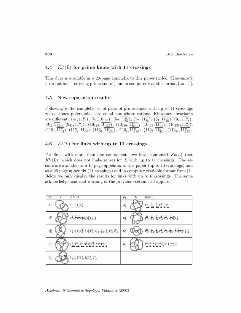
4.6 Kh(L) for links with up to 11 crossings

For links with more than one components, we have computed Kh(L) (notKh′(L), which does not make sense) for L with up to 11 crossings. The re-sults are available as a 16 page appendix to this paper (up to 10 crossings) andas a 26 page appendix (11 crossings) and in computer readable format from [1].Below we only display the results for links with up to 6 crossings. The sameacknowledgement and warning of the previous section still applies:

nck

L Kh(L) nck

L Kh(L)

221 10

010212

4126 42

1 14

1214

1013

1012

610410

2

521 1

3

812

612

411

220220

011012

4 621 1

6

1816

1615

1614

1213

1212

810610

4

622 10

210411

412612

813813

10141014

12151416

141616 62

3 16

1615

1415

1214

1224

1023

1012

822

611

410410

2

631 1

6

1515

1134

1134

913

922

712

521

310310

1 632 1

3

722

512

321

140140

121112

322513

7

633 10

310512

7131114

9341124

13



References

[1] This paper’s web site http://www.ma.huji.ac.il/~drorbn/papers/

Categorification/ carries the text of the paper and all programs and datamentioned in it. Much of it also at arXiv:math.GT/0201043 (for programs anddata load the source).

[Ga] S. Garoufalidis, A conjecture on Khovanov’s invariants, University of Warwickpreprint, October 2001.

[HT] J. Hoste and M. Thistlethwaite, Knotscape, http://dowker.math.utk.edu/

knotscape.html

[Ka] L. H. Kauffman, On knots, Princeton Univ. Press, Princeton, 1987.

[Kh1] M. Khovanov, A categorification of the Jones polynomial, arXiv:

math.QA/9908171.

[Kh2] M. Khovanov, A functor-valued invariant of tangles, arXiv:math.QA/0103190.

[Ro] D. Rolfsen, Knots and Links, Publish or Perish, Mathematics Lecture Series 7,Wilmington 1976.

[Sc] R. Scharein, KnotPlot, http://www.cs.ubc.ca/nest/imager/

contributions/scharein/KnotPlot.html

[St] A. Stoimenow, Polynomials of knots with up to 10 crossings, http://

guests.mpim-bonn.mpg.de/alex/

[Wo] S. Wolfram, The Mathematica Book, Cambridge University Press, 1999 andhttp://www.wolfram.com/.

Institute of Mathematics, The Hebrew UniversityGiv’at-Ram, Jerusalem 91904, Israel

Email: [email protected]

URL: http://www.ma.huji.ac.il/~drorbn

Received: 13 January 2002


370 Dror Bar-Natan

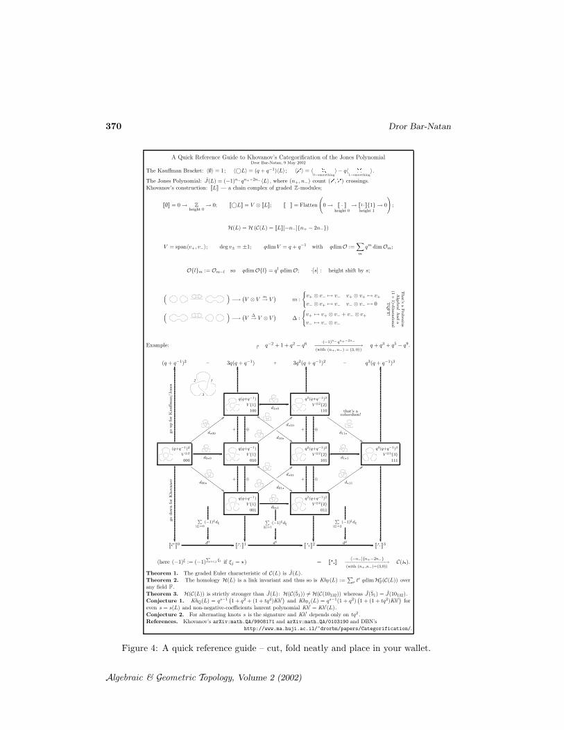
A Quick Reference Guide to Khovanov’s Categorification of the Jones PolynomialDror Bar-Natan, 9 May 2002

The Kauffman Bracket: 〈∅〉 = 1; 〈©L〉 = (q + q−1)〈L〉; 〈0〉 = 〈 10−smoothing

〉 − q〈 H1−smoothing

〉.

The Jones Polynomial: J(L) = (−1)n−qn+−2n−〈L〉, where (n+, n−) count (!,") crossings.Khovanov’s construction: JLK — a chain complex of graded Z-modules;

J∅K = 0 → Zheight 0

→ 0; J©LK = V ⊗ JLK; J0K = Flatten

(

0 → J1Kheight 0

→ JHK{1}height 1

→ 0

)

;

H(L) = H (C(L) = JLK[−n−]{n+ − 2n−})

V = span〈v+, v−〉; deg v± = ±1; qdimV = q + q−1 with qdimO :=∑

m

qm dimOm;

O{l}m := Om−l so qdimO{l} = ql qdimO; ·[s] : height shift by s;

( )

−→(

V ⊗ Vm→ V

)

m :

{

v+ ⊗ v− 7→ v− v+ ⊗ v+ 7→ v+

v− ⊗ v+ 7→ v− v− ⊗ v− 7→ 0

( )

−→(

V∆→ V ⊗ V

)

∆ :

{

v+ 7→ v+ ⊗ v− + v− ⊗ v+

v− 7→ v− ⊗ v−

That’s

aFro

ben

ius

Alg

ebra

!A

nd

a(1

+1)-d

imen

sional

TQ

FT

!

Example:�

q−2 + 1 + q2 − q6 ·(−1)n− qn+−2n−

−−−−−−−−−−−−−−→(with (n+, n−) = (3, 0))

q + q3 + q5 − q9.

(q + q−1)2 −

1

3

2

3q(q + q−1) + 3q2(q + q−1)2 − q3(q + q−1)3

q(q+q−1)

V {1}

100

◦d1⋆0

//

◦

HHHH

HHHH

d10⋆ ##HHHH

HHHH

OO

+ ⊕

q2(q+q−1)2

V ⊗2{2}

110 that’s acobordism!

d11⋆

$$IIIIIIIIIIIIIIIII

OO

+ ⊕

(q+q−1)2

V ⊗2

000

d⋆00

;;wwwwwwwwwwwwwwwww

d0⋆0

//

d00⋆

##GGGG

GGGG

GGGG

GGGG

G

go

up

for

Kauffm

an/Jones

OO

go

dow

nfo

rK

hov

anov

��

q(q+q−1)

V {1}

010

d⋆10

;;vvvvvvvvvvvvvvvvv

◦

d01⋆ ##HHHHHHHHHHHHHHHHH

+ ⊕

q2(q+q−1)2

V ⊗2{2}

101

◦d1⋆1

//

+ ⊕

q3(q+q−1)3

V ⊗3{3}

111

OO

��

q(q+q−1)

V {1}

001

vvvvvvvv

d⋆01

;;vvvvvvvv

d0⋆1

//

��

q2(q+q−1)2

V ⊗2{2}

011

d⋆11

::vvvvvvvvvvvvvvvvv

��J&K0 d0

// J&K1 d1// J&K2 d2

// J&K3

∑

|ξ|=0

(−1)ξdξ

��

∑

|ξ|=1

(−1)ξdξ

��

∑

|ξ|=2

(−1)ξdξ

��

(here (−1)ξ := (−1)∑

i<j ξi if ξj = ⋆) = J&K ·[−n−]{n+−2n−}−−−−−−−−−−−−−→(with (n+,n−)=(3,0))

C(&).

Theorem 1. The graded Euler characteristic of C(L) is J(L).Theorem 2. The homology H(L) is a link invariant and thus so is KhF(L) :=

∑

r tr qdimHrF(C(L)) over

any field F.Theorem 3. H(C(L)) is strictly stronger than J(L): H(C(51)) 6= H(C(10132)) whereas J(51) = J(10132).Conjecture 1. KhQ(L) = qs−1

(

1 + q2 + (1 + tq4)Kh′)

and KhF2(L) = qs−1(1 + q2)

(

1 + (1 + tq2)Kh′)

foreven s = s(L) and non-negative-coefficients laurent polynomial Kh′ = Kh′(L).Conjecture 2. For alternating knots s is the signature and Kh′ depends only on tq2 .References. Khovanov’s arXiv:math.QA/9908171 and arXiv:math.QA/0103190 and DBN’s

http://www.ma.huji.ac.il/~drorbn/papers/Categorification/.

Figure 4: A quick reference guide – cut, fold neatly and place in your wallet.


ISSN 1472-2739 (on-line) 1472-2747 (printed) ATG · PDF fileISSN 1472-2739 (on-line) 1472-2747...

Documents

Transcript of ISSN 1472-2739 (on-line) 1472-2747 (printed) ATG · PDF fileISSN 1472-2739 (on-line) 1472-2747...