ISSN 1198-6727 Fisheries Centre Research Reports · Fisheries Centre Research Reports 1996, Vol.4...
159
Fisheries Centre Research Reports 2002 Volume 10 Number 2 The Use of Ecosystem Models to Investigate Multispecies Management Strategies for Capture Fisheries Fisheries Centre, University of British Columbia, Canada ISSN 1198-6727
Transcript of ISSN 1198-6727 Fisheries Centre Research Reports · Fisheries Centre Research Reports 1996, Vol.4...

Fisheries Centre Research Reports
2002 Volume 10 Number 2
The Use of Ecosystem Models to
Investigate Multispecies Management Strategies for
Capture Fisheries
Fisheries Centre, University of British Columbia, Canada
ISSN 1198-6727

ISSN 1198-6727
The Use of Ecosystem Models to Investigate Multispecies Management Strategies
for Capture Fisheries
Fisheries Centre Research Reports 2002 Volume 10 Number 2

edited by
Tony Pitcher and Kevern Cochrane
156 pages © published by
The Fisheries Centre, University of British Columbia
2204 Main Mall
Vancouver, B.C., Canada 2002
ISSN 1198-6727

THE USE OF ECOSYSTEM MODELS TO INVESTIGATE MULTISPECIES
MANAGEMENT STRATEGIES FOR CAPTURE FISHERIES
Edited by
Tony Pitcher and Kevern Cochrane 2002
Fisheries Centre Research Reports 10(2),156pp
CONTENTS Page
Directors Foreword Ecosim and the Land of Cockayne ....................................................... 3 Executive Summary .................................................................................................................. 4 Introduction The Use of Ecosystem Models to Investigate Ecosystem-Based Management Strategies for Capture Fisheries: Introduction Kevern Cochrane ................................................................................................................. 5 Searching for Optimum Fishing Strategies for Fishery Development, Recovery and Sustainability Carl J. Walters, V. Christensen and Daniel Pauly ........................................................... 11 Contributed Papers
Simulating Fisheries Management Strategies in the Strait of Georgia Ecosystem using Ecopath and Ecosim Steven J. D. Martell, Alasdair I. Beattie, Carl J. Walters, Tarun Nayar and Robyn Briese .........................................................................................16 The Use of Ecosystem-based Modelling to Investigate Multi-species Management Strategies for Capture Fisheries in the Bali Strait, Indonesia Eny Anggraini Buchary, Jackie Alder, Subhat Nurhakim and Tonny Wagey.............. 24 The Eastern Bering Sea Kerim Aydin ................................................................................................................ 33 A Preliminary North-East Atlantic Marine Ecosystem Model: the Faroe Islands and ICES Area Vb Dirk Zeller and Katia Freire ..................................................................................... 39 Policy Simulation of Fisheries in the Hong Kong Marine Ecosystem Wai-Lung Cheung, Reg Watson and Tony Pitcher........................................................... 46 Exploration of Management and Conservation Strategies for the Multispecies Fisheries of Lake Malawi using an Ecosystem Modelling Approach Edward Nsiku ................................................................................................................ 54 The Use of Ecosim to Investigate Multispecies Harvesting Strategies for Capture Fisheries of the Newfoundland-Labrador Shelf Marcelo Vasconcellos, Johanna Heymans and Alida Bundy ..........................................68 Simulating Management Options for the North Sea in the 1880s Steven Mackinson............................................................................................................... 73 Ecosim Case Study: Port Phillip Bay, Australia Beth Fulton and Tony Smith ..............................................................................................83

Page 2, Using Ecosim for Fisheries Management
Simulating Extreme Fishing Polices in Prince William Sound, Alaska: a preliminary evaluation of an ecosystem-based policy analysis tool Thomas A. Okey ...........................................................................................................................94 Exploring Alternative Management Policies: A Preliminary Ecological Approach for the San Matias Gulf Fishery, Argentina Villarino María Fernanda, Mario L. Lasta and Marcelo Pájaro...................................... 109 Exploring Multispecies Harvesting Strategies on the Eastern Scotian Shelf with Ecosim Alida Bundy and Sylvie Guénette ............................................................................................ 112 The Use of Ecosystem Models to Investigate Multispecies Management Strategies for Capture Fisheries: Report on Southern Benguela Simulations Lynne Shannon ............................................................................................................... 118 Impact of Harvesting Strategies on Fisheries and Community Structure on the Continental Shelf of the Campeche Sound, Southern Gulf of Mexico Francisco Arreguin-Sanchez ............................................................................................127 Evaluating Harvesting Strategies for Fisheries of the Ecosystem of the Central Gulf of California Francisco Arreguín-Sánchez and Luis E. Calderón-Aguilera ........................................ 135 Testing Responses of a Tropical Shelf Ecosystem to Fisheries Management Strategies: a Small-scale Fishery from the Colombian Caribbean Sea Luis Orlando Duarte and Camilo B. García ....................................................................142 Exploratory analysis of possible management strategies in Lake Victoria fisheries (Kenyan sec-tor) using the recent Ecosim software Jacques Moreau and Maria Concepcion Villanueva ....................................................150 Participants in the Workshop ............................................................................................. 155
This report is co-published as an FAO Fisheries Report
A Research Report from The UBC Fisheries Centre and the Food and Agriculture Organisation of the United Nations
156 pages © Fisheries Centre, University of British Columbia, 2002

FAO/Fisheries Centre Workshop, Page 3
Director’s Foreword Ecosim in the Land of Cockayne There is a famous Breughal engraving, ‘Big Fish Eat Little Fish’, that illus-trates a marine food web by showing how the stomach of each size of fish contains fish of the smaller size class below. I use it to dramatise trophic re-lationships and, many years ago, it made a neat cover for my textbook (Pitcher and Hart 1982). One student later said that the book cover taught him all he knew. Another Breughal painting is reproduced opposite in hopes it will be equally instructive. Like the Breughal engraving, Ecopath models take all trophic relationships within an aquatic ecosystem into ac-count, and the approach will be famil-iar to many readers of Fisheries Cen-tre Research Reports, being the sub-ject of 5 previous issues from 1996 (see below). Ecosim, the dynamic version of Eco-path (Walters et al. 1997, 2000) has recently been endowed with routines that not only simulate the consequences of changes in fisheries for all ele-ments in the ecosystem, but can also search for fishing rates that will maximize ecological, social or economic goals. The first report of this impor-tant advance made by Carl Walters is presented here. This new facility has interested FAO because it could lead to a way of managing multispecies fisheries that takes into consideration all ele-ments of the ecosystem, not just those that are subjected to fishing. Hence, the Fisheries Centre and FAO decided to hold a workshop to explore the potential of the new software, and the papers in this report are the result. Back to that Breughal. The ‘Land of Cockayne’ is a derisive medieval comment on those who imagine themselves in a paradise where food and luxuries are so easily obtainable that life is comprised of little more than a happy indolence. Or boast that they are in such a place. As Breugal’s painting shows (above), Cockayne is evidently such a fool’s paradise. The term ‘Cockayne’ probably derives from ‘cake’ (OED), and there are similar terms in medieval French. It gave rise to ‘Cockneys’, in-habitants of London noted for boasting of the mi-raculous nature of their city, and a similar idea
also became the ‘Big Rock Candy Mountain’ of US hobo lore. What’s the moral here? Well - it is all too easy to be seduced by these elegant simulations. The ‘Land of Cockayne’ is intended to provide a plan-gent warning that we should continually check simulation results with the real world. And not be tempted to boast that Ecosim optima place us in a far better world. It is a reality check. The Fisheries Centre Research Reports series publishes results of research work carried out, or workshops held, at the UBC Fisheries Centre. The series focusses on multidisciplinary problems in fisheries management, and aims to provide a syn-optic overview of the foundations, themes and prospects of current research. Fisheries Centre Research Reports are distributed to appropriate workshop participants or project partners, and are recorded in the Aquatic Sci-ences and Fisheries Abstracts. A full list appears on the Fisheries Centre's Web site, www.fisheries.ubc.ca. Copies are available on re-quest for a modest cost-recovery charge. Tony J. Pitcher
Professor of Fisheries Director, UBC Fisheries Centre
The Land of Cockayne, by Pieter Breughal the Elder, 1567. As well as illustrating a Fool’s Paradise (note the egg on legs and the walking roast pig), the painting also shows how some of the workshop par-ticipants felt after a week of simulations.
Oil on panel, 52 x 78 cm, Alte Pinakothek, Munich.

Page 4, Using Ecosim for Fisheries Management
Literature cited Pitcher, T.J. and P.J.B. Hart (1982) Fisheries Ecology.
Chapman and Hall, London. 414 pp Walters, C., Christensen, V., and Pauly, D. (1997) Struc-
turing dynamic models of exploited ecosystems from trophic mass-balance assessments. Reviews in Fish Biology and Fisheries 7(2): 139-172.
Walters, C., Pauly, D., Christensen, V., and Kitchell, J. F. (2000) Representing density dependent conse-quences of life history strategies in aquatic ecosys-tems: EcoSim II. Ecosystems 3(1): 70-83.
Mass-Balance Models of North-eastern Pacific Ecosys-tems. Fisheries Centre Research Reports 1996, Vol.4 (1), 131 pp.
Use of Ecopath with Ecosim to Evaluate Strategies for Sustainable Exploitation of Multi-Species Re-sources. Fisheries Centre Research Reports 1998, Vol.6 (2), 49 pp
A Trophic Mass-Balance Model of Alaska's Prince Wil-liam Sound Ecosystem for the Post-Spill Period 1994-1996. Fisheries Centre Research Reports 1999, Vol.6 (4), 143 pp
Ecosystem Change and the Decline of Marine Mam-mals in the Eastern Bering Sea. Fisheries Centre Research Reports 1999, Vol.7 (1), 106 pp.
A Trophic Mass-Balance Model of Alaska's Prince Wil-liam Sound Ecosystem for the Post-Spill Period 1994-1996, 2nd Edition. Fisheries Centre Research Reports 1999, Vol.7 (4), 137 pp.
Executive Summary This report comprises the edited proceedings of workshop held at the Fisheries Centre, University of British Columbia in July 2000, jointly spon-sored by FAO, Rome and thr government of Ja-pan. This is the first published account of new Ecosim policy search software that aims to find fishing rates that maximize objective functions for eco-nomic, ecological, employment or mixed goals. Two papers set out the numerical basis for the software and the procedure that was adopted for the workshop case studies. The report contains 18 case study papers explor-ing the use of the ecosim policy software. Papers examine fisheries and their ecosystems in the Strait of Georgia (BC), the Bali Strait (Indone-sia), the North Sea, The Faroe Islands, Hong Kong, Lake Malawi, Newfoundland, Port Philip Bay (Tasmania), Prince William Sound (Alaska), the San Matias Gulf (Argentina), the Scotian Shelf (Canada), Southern Benguela (South Africa), Campeche Sound (Mexico), Gulf of California (Mexico), the Caribbean (Columbia).

FAO/Fisheries Centre Workshop, Page 5
The Use of Ecosystem Models to Investigate Ecosystem-based Management Strategies for Capture Fisheries: Introduction Kevern L. Cochrane FAO, Rome The Rationale: Providing Scientific Information for Management In recent years those involved in the utilisation and management of aquatic resources have come to realise that the single-species or -resource ap-proach still prevailing in the vast majority of fish-eries in the world is incomplete and inadequate. Faced with mounting evidence of failures in our on-going attempts to use living aquatic resources in a sustainable and responsible way, we have been forced to re-examine the science, the man-agement and the operations applied in fisheries, and all three have been found to be lacking. One of the most fundamental deficiencies is now widely considered to be the tendency to focus on fishery resources as essentially independent stocks, driven entirely by their inherent popula-tion dynamics, as has been the practice during the dramatic expansion in fishing power and catches that characterised fisheries in the 20th Century. In response to this realisation, global attention within fisheries is turning towards recognising that biological populations and communities function within and are ultimately regulated by the ecosystems in which they occur. The challenge now is to translate this intellectual acceptance of the need to manage fisheries as integral parts of the ecosystem, into an effective methodology that allows us to make optimal use of our diverse aquatic ecosystems in a responsible and sustain-able way. The principles of ecosystem-based management of fisheries incorporate and extend the conven-tional principles for sustainable fisheries devel-opment. Instead of focusing on a single-species, ecosystem-based fisheries management strives to consider the capacity of the ecosystem as a whole to produce food, revenues, employment and other essential and desirable services for humankind. From that starting point, it is necessary to devise utilisation and management strategies that enable us to optimise that capacity, taking into account variability in the system and uncertainty in our knowledge. Instead of setting only relatively sim-
ple reference points related to single populations, these strategies will also need to refer to limits and targets related to conservation of ecosystem components, structures, processes and interac-tions. An immediate implication of this is that the complexity of the system we are considering in-creases and the number of objectives and the con-flicts between those objectives increases substan-tially. This expansion in uncertainty and com-plexity is not, however, a consequence of adopting ecosystem-based management, it is the result of recognising and attempting to consider the full complexity and uncertainty that have always been there, but that we have previously ignored. Fishery scientists, managers and interest groups are generally aware of the need to consider this full range of complexity, but there is still preva-lent ignorance as to how to implement an effec-tive ecosystem-based management system in practice, and the practical problems raised by this recognition are considerable. Uncertainties and conflicting objectives have severely hindered suc-cessful application of efforts to implement single-species management and will be even harder to deal with as ecosystem interactions are recog-nised and incorporated. Both the need for and difficulty of ecosystem-based fisheries management were recognised by the 95 States which met in Kyoto, Japan, from 4 to 9 December 1995 on the occasion of the Inter-national Conference on the Sustainable Contribu-tion of Fisheries to Food Security. They formu-lated the Kyoto Declaration which proposed, amongst other important principles, that States should base their fisheries ‘policies, strategies and resource management and utilization for sustain-able development of the fisheries sector on the following: (i) maintenance of ecological systems; (ii) use of the best scientific evidence available; (iii) improvement in economic and social well-being; and (iv) inter- and intra-generational eq-uity’. Subsequent to the Kyoto Conference, the Gov-ernment of Japan provided financial support to FAO for a programme to assist countries in im-plementing the Kyoto Declaration. One of the projects undertaken under this programme was entitled “Multispecies Fisheries Management” and aimed to investigate methods of providing scientific advice for improved multispecies and ecosystem-based fisheries management. Under this project, a workshop was held at the Fisheries Centre, UBC, in March 1998 to consider the “Use of Ecopath with Ecosim to Evaluate Strategies for Sustainable Exploitation of Multispecies Re-

Page 6, Using Ecosim for Fisheries Management
sources”1. The workshop did not come up with formal conclusions and recommendations, but there was widespread agreement that Ecopath with Ecosim (EwE), as a well-developed and ge-neric ecosystem-modelling tool, could play a use-ful role in providing important information to de-cision-makers on fisheries policy and strategies from an ecosystem perspective, complementary to that available from conventional single-species assessments. This second workshop, also supported by the Government of Japan, was designed to follow-on from that preliminary meeting and to look in more detail, using specific case studies, at the type of information, including its limitations, which can be expected from our existing ability to assess and forecast at the scale of ecosystems. The Objective of the Workshop A key requirement for effective management is good information upon which good decisions can be based, and it is a key role for science and scien-tists to provide the best available information on the state of the resources and their likely re-sponse, or responses, to any planned fisheries or management action. The workshop was intended primarily to address this task and, particularly, to examine the nature of the information at the scale of the ecosystem which scientists can provide for ecosystem-based fisheries management. The objective of the workshop was therefore to use quantitative ecosystem models to investigate the impact of different multispecies harvesting strategies on the community structure and fishery yields of different ecosystem types with a view to identifying preferred harvesting strategies. The starting point of the workshop was the mod-els we have available. The workshop was open to any interested scientist who had been working on ecosystem modelling, and each participant was asked to bring a working ecosystem model of an exploited aquatic ecosystem, including the impact of the fishery or fisheries on exploited stocks. In practice, all the models brought to the workshop were EwE models. The participants were also asked to bring, as far as possible, supplementary information which could be used to assist in evaluating and developing realistic management objectives and strategies for their particular eco-system. This supplementary information in-cluded, for example, estimates of pristine biomass
1 Use of Ecopath with Ecosim to Evaluate Strategies for Sus-tainable Exploitation of Multispecies Resources. Fisheries Centre Research Reports 6 (2). Fisheries Centre, University of British Columbia, Vancouver. 49pp.
of the different stocks or a suitable surrogate of such estimates, background information on the social and economic importance of the fishery, and estimates of bycatch, discards and unre-ported catch. These models and information were to be used by each participant:
to consider different sets of objectives for their ecosystem; to use the models to identify the management strategies which would come closest to achiev-ing those objectives; and to estimate the ecosystem consequences of each management strategy.
In doing so, the participants were also asked to consider the key sources of uncertainty in their models and the possible implications of these for their results and conclusions. This approach effectively uses the ecosystem models as operating models (e.g. Hilborn and Walters, 1992; Cochrane et al., 1998). Such an application was one of the primary goals of the developers of Ecosim, who suggested it could be used to “conduct fisheries policy analyses that ex-plicitly account for ecosystem trophic interac-tions” (Walters et al. 1997) and routines have been provided in Ecosim to assist the user in such exploration of fisheries strategies or policies. A full description of these routines can be found in the Help System of EwE. The first of the routines is the ‘open loop’ policy search which estimates the time-series of relative fleet sizes that would maximize a multi-criterion objective function that includes net economic value, social employment value, and ecological stability criteria. The relative fleet sizes are used to calculate the relative fishing mortality rates by each fleet type on the affected stocks. The user, in this case the participant at the workshop, could therefore specify the relative priority of economic value, social employment value and ecosystem stability, where ecosystem stability can be defined in terms of relative abundance of the different biological groups included in the model. These relative priorities represent the management goals. The open loop search then identifies the strategy, in terms of relative fleet sizes, that comes closest to meeting those goals. Ecosim also includes ‘closed loop’ policy simula-tions that allow the user to examine the conse-quences of a given management strategy, taking into account the dynamics and uncertainties of the stock assessment and regulatory processes.

FAO/Fisheries Centre Workshop, Page 7
In order to do this, it includes routines to simu-late the dynamics of the assessment process, i.e. collection of data including errors in the estimates of biomass or fishing rate, and for the implemen-tation of the assessment results through limita-tion of the annual fishing efforts. Developing the Strategies at the Workshop Determining Strategies for Base Case Management Objectives It is possible to use EwE to explore policy options in a variety of ways but it was decided that the routines included in EwE for this purpose, the ‘open loop’ search and the ‘closed loop’ simula-tions, would be the primary tools used at this workshop. The open loop routine uses a non-linear search procedure to determine the optimum fishing rates over time across the fleet, according to the objec-tive function specified by the user in the open loop input screen (Table 1). The closed loop routine uses the fishing pattern identified as optimum for a specified management goal using the open loop, and then runs a se-ries of forward projections us-ing that fishing pattern but maintaining the target fishing rates of the different fleets in accordance with the annual observations, with specified errors, on the status of the stock. This routine enables the user to estimate the actual per-formance of the selected man-agement strategy (i.e. the op-timum fishing pattern over time estimated by the open loop routine) given the obser-vation error inevitably en-countered by the fisheries manager striving to maintain the fishing rates specified by the policy in a real fishery. The information generated by these routines could be used, in combination with other sources of information includ-ing the results of single-species assessments and fore-
casts, to inform the manager on the strategy or strategies that would best achieve the agreed ob-jectives. Strategies Considered As a common starting point, participants were asked to investigate strategies that would achieve five “base case” management objectives, of which three (b – d below) were derived directly from the options available in the open loop routine. The base case strategies were: a) current fishing strategy; b) maximum economic value; c) maximum employment; d) maintaining ecosystem structure; and e) the “big compromise”: giving equal priority to
achieving economic; employment and ecosystem structure performance.
The strategies b), c) and d) were considered to be extremes and unlikely to be seriously considered as realistic options in the ecosystems being stud-
Value Component Value Weight Net economic value 0.01 Net social (employment) value
0.01
Ecosystem stability 1
a) Determining broad policy priorities
Gear Type Jobs/Catch Purse seine 0.02 Bottom trawl 0.03 Long line 0.1
b) Specifying the relative employment value of the different fisheries indicating
which fisheries will be favoured under Net social value
Biomass group B ideal / B base Importance Phytoplankton 1 0.01 Sardine 1.5 1 Hake 2 1
c) The target biomass (B ideal / B base) and relative Importance of the different
biomass groups to specify what ecosystem structure is preferred under Ecosystem Stability
Table 1. The inputs required to specify a management goal under the open loop routine. The entries shown are hypothetical and given as examples only. With those given under Table 1a), the objective non-linear search procedure would attempt to determine the fishing rate pattern which maintained ecosys-tem stability in accordance with the targets and Importance scorings given in Table 1c.

Page 8, Using Ecosim for Fisheries Management
ied. However, examining the implications of each was considered to be informative and the extreme boundaries they represented could provide useful starting points from which to consider multi-objective strategies, such as the ‘big compromise’. When considering objectives and strategies for in-forming managers, as opposed to the exploratory trials undertaken at the workshop, the open loop routine of EwE could be used to explore a wide range of more subtle compromises between the basic Value Components of economic value, social value and ecological stability (Table 1a). Procedure for Identifying Strategies The following specifications and procedures were agreed upon to ensure reliability and comparabil-ity in results of this investigation. • All strategies would be tested over a 20 year
simulation unless the results indicated that the ecosystem had not stabilised over that pe-riod, in which case the simulation period would be extended until stability was achieved.
• With any non-linear search procedure, there
is a danger that the procedure will converge on a local minimum, not on the global mini-mum for the given objective function. Par-ticipants were therefore advised to undertake at least 5-6 separate estimations using the “start at random F’s” option in the routine and to check the value of the objective func-tion after each to ensure that the procedure has reached a global minimum.
• Sensitivity analyses were undertaken to in-
vestigate the effect of the vulnerability set-tings used in the simulations as output from Ecosim is particularly sensitive to these val-ues. These were to include options with vul-nerability set at 0.4 and 0.7 throughout, as well as any matrix of settings assumed or es-timated for that specific ecosystem.
• A discount rate of 0.04 would be used as the
default value in the open loop searches. The fishing rates per fleet, catches obtained, eco-nomic values obtained, biomass of the key bio-mass groups and value of the objective function, including for each Value Component (i.e. eco-nomic value, social value and ecosystem stability), were noted for each open loop estimation. Testing the performance of the current fishing strategy in each ecosystem (option a) required running the model over the 20 year simulation
with the fishing rates of each fleet maintained at the rates used in the underlying Ecopath model. Maximising the economic value, employment or maintaining ecosystem structure required speci-fying a weight of 1 for the appropriate Value Com-ponent shown in Table 1 a), and low, non-zero values (e.g. 0.01) for the other two. Under the “big compromise” it was found that the objective function used in the search procedure generated a negatively biased weight for ecosystem stability and therefore, instead of using equal weights for each of the three Value Components under this scenario, it was found necessary to give weights of, for example, 1 to each of Economic value and Social value but a higher weight (typically between 5 and 25) to ecosystem stability in order to achieve an objective function that generated the desired compromise. The problem is well illustrated in, for example, the chapters by Vasconcellos et al. (see Figure 3) and Bundy (see Figures 2 and 3). In both cases the authors demonstrate the affects of changing the weighting given to the ecosystem value com-ponent relative to the other value components and discuss the difficulties associated with identi-fying an appropriate ecosystem weighting. In other cases authors selected a single weighting which generated a solution in which an accept-able level of ecosystem stability was achieved, while in other cases authors simply used a weighting of one. In these last cases, there is a high probability that the ecosystem stability crite-rion was dominated by the economic and social value components and that the estimated strategy would not, in fact, achieve the desired result. This workshop helped to demonstrate the prob-lems in the optimisation routine and to point to ways of addressing it. At the time of the finalisa-tion of this report, suitable mathematical solu-tions are being considered and may be included in the EwE software in due course. Defining ‘Ecosystem Stability’ In addition to the mathematical problem just de-scribed, a fundamental philosophical issue also arose at the workshop. In discussions on appro-priate values to use for the input screen reflected in Table 1 c), it became apparent that the term “Ecosystem Stability” did not mean the same to all participants and that what was considered to be the desired state for an ecosystem was highly subjective. In a policy that excluded fishing, it may be reasonable to specify the desired state by giving all biomass groups equal weight, and indi-cating the desired B(ideal) for each group as be-ing the estimated pristine biomass (i.e. prior to

FAO/Fisheries Centre Workshop, Page 9
fishing). However, shutting down all the fisheries is only rarely a preferred management option and fishing is an integral part of most ecosystems. Fishing must inevitably result in a reduction in biomass of the groups caught by the fishing gear and is also likely to lead to perturbations in other groups. The pristine option is therefore excluded as a feasible goal and the user (or manager in a real fishery) has to identify a generally-acceptable desired state for the ecosystem and its component parts in the presence of fishing. Just what that desired state will be will frequently prove to be controversial, as was found at the workshop. Here, opinions ranged from: uniform reduction to the same (as a proportion of pristine) precautionary sustainable level in all biomass groups (the ‘ecosystem as the sum of its parts’ view); maintaining the key exploited groups at their most productive levels (the sustainable utili-zation view); to striving to maintain species of particular conservation interest, such as cetace-ans and turtles, at the highest levels relative to their pristine biomass (the conservationist view). This matter was not finally resolved at the work-shop and reflects an important source of potential conflict as fisheries move towards ecosystem-based management. At the workshop, partici-pants therefore tended to explore their own pre-ferred options when considering ecosystem sta-bility. This freedom of choice will not be a possi-ble option, however, when different user groups are competing for the same resources in an eco-system! Testing the Strategy with Observation Error: the closed loop Once the optimum management strategy had been identified for a given set of objectives, it was then tested for performance in simulations of 20 years in the presence of observation error using the closed loop routine. Under this, the strategy was run 100 times with randomly generated ob-servation error in the index of abundance of each biomass group used each year by the ‘manager’ in order to maintain the fishing rates at those speci-fied in the strategy. These indices could be speci-fied as either estimated catch or biomass, or the directly estimated exploitation rate of the previ-ous year arising from, for example, a tagging pro-gramme. The closed loop routine therefore al-lows the user to estimate the affects of observa-tion and implementation error on the perform-ance of the strategy identified by the open loop search. At the end of each set of Monte Carlo runs, par-ticipants were requested to record the value of the
objective function for each of the three Value Components for comparison with the results ob-tained in the open loop routine, and also to de-termine the spread of the biomass trajectories for each biomass group. The Wise Usxe of Policy Search Routines The results of the workshops clearly illustrated the valuable role of the open and closed loop pol-icy search routines in exploring ecosystem-based management strategies. These routines provide efficient and objective means of identifying strategies that will best achieve clearly specified and precise objectives. However, many of the pa-pers also illustrate the absolute need to interpret the results cautiously, taking full account of the uncertainties in both the underlying model and in the optimisation routine itself. The impact of the weighting factor for the ecosys-tem value component has already been discussed. Similarly the need to initiate the open loop rou-tine with different starting values of F to ensure that the optimisation was converging on a global minimum was stressed at the start of the work-shop. The importance of doing this is well illus-trated in the chapter by Mackinson. In his study he demonstrated that different starting values of F generated considerably different estimates of the optimal management strategy and he used these results to identify an initialisation option and procedure that achieved consistent results. The sensitivity of the model behaviour to the as-sumed values of the vulnerability settings was also stressed at the outset of the workshop and this is clearly illustrated in several of the chapters, including those by Martell and his co-authors, Buchary et al., Mackinson and Shannon. Shan-non, for example, estimated optimal fishing mor-talities for the pelagic fleet in the southern Ben-guela ecosystem that varied by a factor of ap-proximately 6 in order to achieve the ‘compro-mise’ strategy, depending on whether the vulner-ability factor was set at 0.4 or 0.7 across the eco-system. Mackinson suggested that there was no clear pattern in the relationship between flow control and the estimated resilience of a species or species group to fishing and he advised caution in interpretation, suggesting that ‘once a particu-lar policy has been chosen, the response to changes in the assumptions of flow control should be thoroughly examined’. The implications of this are that the different policies, or strategies, being considered need to be examined in an iterative manner, comparing their performance under a range of sensitivity tests. The final strategy to be selected must be the one that performs best under

Page 10, Using Ecosim for Fisheries Management
the range of feasible parameter values and as-sumptions, and that is robust to the major uncer-tainties. The overall conclusions for anyone considering using the EwE policy search routine to explore possible management strategies seriously is that it is a powerful and sophisticated tool, and there-fore, as with all comparable models, one that needs to be used carefully and with common sense, not as a simple recipe book. The user must be conversant with the principles of non-linear optimisation and must follow the practices and guidelines that apply to such statistical tests. Without cautious, thoughtful and active use of the software, the probability of dangerously mislead-ing results and conclusions is far greater than that of obtaining sensible and meaningful informa-tion. Reporting The results of the investigations described above are discussed in this Report under the chapters prepared by the participants on the ecosystem they were working with. In some cases, the au-thors were able to undertake the basic simula-tions and sensitivity tests described above and to go beyond, considering other, more site-specific, management objectives. In other cases the par-ticipants found they did not have the time to go beyond the common base-case simulations. Given these discrepancies in progress, it was not possi-ble at the workshop to complete the final task that had been planned, which was to examine the re-sults of the simulations for the different ecosys-tems to see whether any common or emergent properties could be identified across ecosystems. However, some authors are continuing their in-vestigations and it is planned to publish these ex-tended investigations as a book, including an overall comparison and synthesis based on those on-going investigations. References Cochrane, K. L., Butterworth, D. S., De Oliveira, J. A.
A., and Roel, B. A 1998. Management procedures in a fishery based on highly variable stocks and with conflicting objectives: experiences in the South Af-rican pelagic fishery. Reviews in Fish Biology and Fisheries, 8: 177-214.
Hilborn, R., and Walters, C. J. 1992. Quantitative fish-eries stock assessment. Choice, dynamics and un-certainty. Chapman & Hall, New York. 570 pp.
Walters, C., V. Christensen and D. Pauly 1997. Struc-turing dynamic models of exploited ecosystems from trophic mass-balance assessments. Reviews in Fish Biology and Fisheries 7: 139-172.
FAO/Fisheries Centre Workshop, Page 11
Searching for optimum fishing strategies for fishery development, recovery and sustainability Carl J. Walters, V. Christensen and Daniel Pauly Fisheries Centre, UBC Abstract Policy may be defined as an approach towards reaching a broadly defined goal. In fisheries, policies are often implemented via total allowable catches, TACs, that are recalculated annually, and through regulations that af-fect fleet and deployment. The task of fisheries scien-tists should be to advise both on policy formulation and on its implementation. However, so far ecosystem-based policy explorations have rarely been conducted. This can, however, now be addressed by the recent de-velopment of a policy exploration routine for the Eco-path with Ecosim approach and software. The paper gives an overview of the background for the policy search, and how it has been implemented. A brief over-view of a new routine for examining uncertainty in the management process is also included. On Policy Exploration using Ecopath with Ecosim (EwE) A central aim of fisheries management is to regu-late fishing mortality rates over time so as to achieve economic, social, legal and ecological sus-tainability objectives. An important dynamic modeling and assessment objective is to provide insight about how high these mortality rates should be, and how they should be varied over time (at least during development or recovery from past overfishing). We cannot expect models to provide very precise estimates of optimum fishing mortality rates, but we should at least be able to define reasonable and prudent ranges for the rates. The impacts of alternative time patterns of fishing mortalities can be explored using two different approaches in Ecosim: 1. Fishing rates can be ‘sketched’ over time in the Ecosim simulation interface, and simulated results (catches, economic performance indica-tors, biomass changes) examined for each sketch. This is using Ecosim in a ‘gaming’ mode, where the aim is to encourage rapid exploration of op-tions. 2. Formal optimization methods can be used to search for time patterns of fishing rates (actually, relative fishing efforts by fishing fleet/gear types), which would maximize particular performance
measures or ‘objective functions’ for manage-ment. These approaches can be used in combination, e.g. by doing a formal optimization search then ‘reshaping’ the fishing rate estimates from this search in order to meet other objectives besides those recognized during the search process. The first of these approaches is what has up to now been the standard simulation form in Eco-sim, and does not require further description here, (see Walters et al., 1997; Christensen et al., 2000; Walters et al., 2000). The newly added formal optimization involves three steps: 1. Define blocks of fleet/year groupings to be in-cluded in the search procedure; 2. Define objective function weights for the four optimization objectives:
(i) net economic value (total landed value of catch minus total operating cost to take this landed value);
(ii) employment (a social indicator, assumed pro-portional to gross landed value of catch for each fleet with a different jobs/landed value ratio for each fleet);
(iii) mandated rebuilding of target species (obtained by setting a threshold biomass for the relevant species relative to their biomass in Ecopath);
(iv) ecological ‘stability’ (measured by assign-ing a weighting factor to each group based on their longevity, and optimizing for the weighted sum).
3. Invoke the search procedure by clicking the search button. When a search has been completed, the resulting ‘optimum’ fishing rates by year/fleet block are transferred to the Ecosim ‘Temporal Simulation’, where the optimized fishing rates will have re-placed the baseline (or previously sketched) rela-tive efforts by fleet/gear type. Methodology Invoking the search option causes Ecosim to use a nonlinear optimization procedure known as the Davidson-Fletcher-Powell (DFP) method to itera-tively improve an objective function by changing relative fishing rates, where each year/fleet block defines one parameter to be varied by the proce-dure, (e.g., setting four color code blocks means a 4-parameter nonlinear search). DFP runs the Ecosim model repeatedly while varying these pa-rameters. The parameter variation scheme used by DFP is known as a ‘conjugate-gradient’ method, which involves testing alternative parameter values so as to locally approximate the objective function as a

Page 12, Using Ecosim for Fisheries Management
quadratic function of the parameter values, and using this approximation to make parameter up-date steps. It is one of the more efficient algo-rithms for complex and highly nonlinear optimi-zation problems like the one of finding a best fish-ing pattern over time for a nonlinear dynamic model. Nonlinear optimization methods like DFP can be tricky to use, and can give grossly misleading re-sults. In particular the method can ‘hang up on a local maximum’, and can give extreme answers due to an inappropriate objective function. To check for false converge to local maxima, an op-tion to use random starting F’s should be used in addition to forcing additional iterations using the option to redo the analysis based on the current F’s. To test for sensitivity of the results to objec-tive function parameters, searches for a variety of values of the objective function weights and pa-rameters should be accessed. The objective function can be thought of as a ‘multi-criterion objective’, represented as a weighted sum of four criterion components or in-dicators: economic, social, legal, and ecological. Assigning alternative weights to these compo-nents is a way to see how they conflict or tradeoff with one another in terms of policy choice. For example: (a) placing a high weight on the net economic value
component (total fishing profits) typically causes the optimization to favor lower fleet sizes and se-vere simplification of the simulated ecosystem to maximize production of only those species that are most profitable to harvest;
(b) placing a high weight on the employment (social)
indicator typically results in favoring larger fleet sizes, and again often severe ecological simplifica-tion in order to maximize production for the fleet that employs the most people.
External pressure, (e.g. in form of legal decisions) may force policy makers to concentrate on pre-serving or rebuilding the population of a given species in a given area. In Ecosim, this corre-sponds to setting a threshold biomass (relative to the biomass in Ecopath) and identifying the fleet structure that will ensure this objective. The im-plication of this policy tends to be case-specific, and to depend on the trophic role of the group whose biomass is to be rebuilt. The ecosystem criterion component is inspired by the work of E.P. Odum (1971) in terms of ‘matur-ity,’ wherein mature ecosystems are dominated by large, long-lived organisms. This is implemented in Ecosim by identifying the fleet structure that
maximizes the biomass of long-lived organisms, as defined by the inverse of their produc-tion/biomass ratios. The optimization of ecosys-tem ‘health’ optimization often implies phasing out of all fisheries except those targeting species with low weighting factors. The search procedure results in what control sys-tems analysts call an ‘open loop policy’, i.e. a pre-scription for what to do at different future times without reference to what the system actually ends up doing along the way to those times. It would obviously be crazy to just apply an open loop policy blindly over time, each year commit-ting a fishery to fishing rates calculated at some past time from only the data available as of that time. In practice, actual management needs to be im-plemented using ‘feedback policies’ where harvest goals are adjusted over time as new information becomes available and in response to unpredicted ecological changes due to environmental factors. But this need for feedback in application does not mean that open loop policy calculations are use-less: rather, we see the open loop calculations as being done regularly over time as new informa-tion becomes available, to keep providing a gen-eral blueprint (or directional guidance) for where the system can/should be heading. Also, we can often gain valuable insight about the functional form of better feedback policies, (how to relate harvest rates to changes in abundance as these changes occur) by examining how the open loop fishing rates vary with changes in abundance, es-pecially when the open loop calculations are done with Ecosim ‘time forcing’ to represent possible changes in environmental conditions and produc-tivity in the future. For an example of this ap-proach to design of policies for dealing with de-cadal-scale variation in ocean productivity for single species management, see Walters and Parma (1996). Maximizing Risk-averse Log Utility for Economic and Existence Values One option in the search procedure for optimum fishing patterns is to search for relative fleet sizes that would maximize a utility function of the form w1⋅log(NPV) + w2⋅S⋅log(B) - w3⋅V, where the wi’s are utility weights chosen by the user, and the utility components NPV, S⋅log(B), and V are de-fined as: (1) NPV is net present economic value of harvests,
calculated as discounted sum over all fleets and times of catches times prices minus costs of fish-ing, i.e., the discounted total profit from fishing the ecosystem.

FAO/Fisheries Centre Workshop, Page 13
(2) S⋅log(B) is an existence value index for all compo-nents of the ecosystem over time. It is calculated as the discounted sum over times and biomass pools of user-entered structure weights times logs of biomasses, scaled to per-time and per-pool by dividing the sum by the number of simulation years and number of living biomass pools.
(3) V is a variance measure for the prediction of
log(NPV) + S⋅log(B). It is assumed to be propor-tional to how severely the ecosystem is disturbed away from the Ecopath base state, where distur-bance is measured at each time in the simulation by the multidimensional distance of the ecosystem biomass state from the Ecopath base state. This term is negative, implying that increased uncer-tainty about the predictions for more severe dis-turbances causes a decrease in the mean of log(NPV). The term represents both aversion to management portfolio choices that have high vari-ance in predicted returns, and the observation that the mean of the log of a random variable (NPV⋅PB) is approximately equal to the log of the mean of that variable minus ½ the variance of the variable. Large w3-values can be used to represent both high uncertainty about predictions that involve large deviations of biomass from the Ecopath base state, and strong risk aversion to policy choices that have high uncertainty.
This utility function combines several basic con-cepts of utility. First, the log scaling of value components represents the notion of “diminish-ing returns”, that adding some amount to any value measure is less important when the value measure is already large than it is when the value measure is small. Second, the log scaling also represents the notion of “balance”, that no value component should be ignored entirely (unless it is assigned a zero wi); the overall utility measure approaches minus infinity if either net economic performance (NPV) or if any biomass component of the ecosystem (any biomass Bi in S⋅log(B)) ap-proaches zero. Third, it represents the notion that our predictions about the future of both economic performance and biodiversity (biomasses) be-come progressively more uncertain for policies that result in more extreme departures from the Ecopath base state about which we presume to have at least some knowledge. In the terminology of portfolio selection theory in economics, fishing policies result in a portfolio of value components with “expected total returns on investment” equal to NPV + S⋅B. But policies that have higher expected total returns are most often also ones that would push the ecosystem into more extreme states, and hence represent portfo-lio choices with higher variance in total returns. For example, maximizing the deterministic pre-diction of NPV in Ecosim often involves a ‘farm-
ing policy’, in which fishing is deployed so as to severely simplify the ecosystem to maximize pro-duction of one or a few species that appear at pre-sent to be the most valuable (price, potential total catch). This may even involve deploying some fleets just to remove predators and competitors for the most valued species, just like deploying pesticides and herbicides to remove “pests” in ag-ricultural systems. But simplifying an ecosystem in such ways can make the behavior of the system deeply unpredictable, by creating opportunities for ecological response (population growth) by a variety of species that are rare in the “normal” ecosystem, and hence are not well researched or understood in terms of their potential impacts on valued species should they become abundant. Simplifying an ecosystem is hence much like in-vesting in high-risk, high-return stock market op-tions; such investments may make you rich, but they may also bankrupt you. Most people are risk-averse as investors, and seek to “spread risk” by investing in “balanced portfolios” with lower expected returns on investment but much lower probabilities of severe loss. The prediction variance measure V is not meant to represent all components of variation or uncer-tainty about future biomasses and fishery values. V goes to zero for policies that hold or maintain the ecosystem at the Ecopath base state Bo for every biomass, for all simulation times. It is ob-viously not correct to suggest that we would ex-pect no variance in future biomasses (and hence in the harvest components of NPV as well) if such a policy were implemented. Imagine running a very large number of simulations of future bio-mass changes under such a policy, while varying all possible uncertain quantities such as the Eco-path base biomasses and biomass accumulation rates, productivities, Ecosim vulnerability pa-rameters, environmental forcing inputs repre-senting oceanographic productivity regimes, fu-ture demand and price patterns, and changing vulnerabilities to fishing due to biophysical and technological factors. Even for the baseline policy where Ecosim predicts stable (‘flat line trajec-tory’) expected or mean biomasses over time, these simulations would likely reveal high vari-ances and complex covariance patterns for most biomasses over time, i.e. we would see wide prob-ability distributions of possible future biomass states for the ecosystem. We should not be arro-gant enough to suggest that we can describe all the uncertainties well enough to accurately calcu-late the variances of such distributions. But note that much of that variance in predictions of future biomasses, (and hence variance in the value com-ponents) would be due to sources of uncertainty

Page 14, Using Ecosim for Fisheries Management
and variability that are the same no matter what the policy choice, i.e., would cause about the same amount of variance in predictions for any future harvest policy that we might simulate. When comparing policy choices using an optimi-zation objective function, there is no point in in-cluding extra constant terms that do not change with the policy variables, (e.g., a base variance Vo in predictions that does not change with fishing rate policy and just represents uncertainty about any prediction that Ecosim might make). Hence the V distance measure is meant to represent only extra variance or uncertainty in predictions for policy scenarios that would likely drive biomasses far from the Ecopath mean state. Note that Ecosim does not deliberately advocate or promote any particular risk-averse portfolio approach to public investment in ecosystem har-vest and existence values. Rather, it provides the logarithmic utility function option so that users who do have highly risk-averse attitudes about ecosystem values can identify policy options that would better meet their objectives. Users should always construct a series of policy scenarios with varying utility weights w1, w2, and w3 on the log utility components, to see how placing different emphases on these components would alter the predicted best policy choice. Use of these functions for policy exploration will generally involve some balance between these ob-jectives. Indeed, identifying the weighting factors to be given to each of these objectives may be the most valuable aspect of this Ecosim routine. Thus, to assist the user in achieving this, the starting values of the objective functions have each been standardized relative to their base val-ues (from Ecopath), making them roughly com-parable. The first two of these measures tend to pull towards increasing fishing effort, while the two others tend to pull towards reducing effort. Care should be taken to consider this balance when giving relative weightings to the objectives. Also note that the optimizations should be per-formed with a range of weighting factors for each objective function, rather than with single values, which may miss a well-balanced solution (see Cochrane, this volume). Open-loop Policy Simulations The fishing policy search interface of EwE de-scribed above estimates time series of relative fleet sizes that maximize a multi-criterion objec-tive function that includes net economic value, social employment value, mandated rebuilding,
and ecological stability criteria. In Ecosim, the relative fleet sizes are used to calculate relative fishing mortality rates by each fleet type, assum-ing the mix of fishing rates over biomass groups remains constant for each fleet type, (i.e. reducing a fleet type by some percentage results in the same percentage decrease in the fishing rates that it causes on all the groups that it catches). The fisheries and ecosystem may be simulated with Ecosim using the solution found in the policy search interface: this is termed an ‘open loop’ simulation. Note that when density-dependent catchability ef-fects are included in the simulations, reductions in biomass for a group may result in fishing rate remaining high despite reductions in total effort by any/all fleets that harvest it. Despite this ca-veat, the basic philosophy in the fishing policy search interface is that future management will be based on control of relative fishing efforts by fleet type, rather than on multispecies quota systems. It is in any case not yet clear that there is any way to implement multispecies quotas safely, without either using some arbitrary conservative rule like closing the fleet when it reaches the quota for the first (weakest) species taken, or alternatively al-lowing wasteful discarding of species once their quotas are reached. If future multispecies management is indeed im-plemented by regulation of fleet fishing efforts so as to track time-varying fishing mortality rate tar-gets as closely as possible, then a key practical is-sue is how to monitor changes in gear efficiency (catchability coefficients) so as to set effort limits each year that account for such changes in effi-ciency. Such monitoring is particularly important for fisheries that can show strong density-dependence in catchability, such that a unit of fishing effort takes a much higher proportion of some stocks (exerts a higher fishing mortality rate per unit of effort) when stock size(s) is/are small. There are at least two possible ways to monitor the changes in catchability (gear efficiency) dis-cussed above. Both are based on monitoring fish-ing mortality rates Ft over time, and using the re-lationship qt=Ft/ft, where qt is fishing rate per unit effort and ft is effort. The first approach is to do traditional biomass stock assessments each year, and to estimate Ft as Ft=Ct/Bt, where Ct is total catch and Bt is esti-mated vulnerable stock biomass. The second ap-proach is to directly monitor the fishing mortality rate, estimating probabilities of harvest using methods such as annual tagging experiments and within-year estimates of relative decrease in fish

FAO/Fisheries Centre Workshop, Page 15
abundance during fishing ‘seasons’. Closed-loop Policy Simulations Ecosim allows users to perform ‘closed loop pol-icy simulations’ to evaluate the monitoring alter-natives discussed above. The evaluations produce time series of biomasses, and also the objective function value components used in searches for optimum long-term fishing rate plans. ‘Closed loop’ simulations model not only the ecological dynamics over time, but also the dynamics of the stock assessment and regulatory process. That is, a closed loop simulation includes ‘submodels’ for the dynamics of assessment (data gathering, ran-dom and systematic errors in biomass and fishing rate estimates) and for the implementation of as-sessment results through limitation of annual fishing efforts. As part of this routine the EwE ‘closed loop policy simulation’ model, allows specification of:
1. how many closed loop stochastic simulation trials to
do; 2. the type of annual assessment to be used (F=C/B ver-
sus F directly from tags); 3. the accuracy of the annual assessment procedures
(coefficient of variation of annual biomass or F esti-mates, by stock); and
4. the value or importance weights for the Fs caused on various species by each fishing fleet.
The value weights are used for each fleet/species combination to calculate a weighted average catchability, qt, for each fleet type, recognizing that some species may be more important than others in terms of the effect that they might be al-lowed to have on effort reduction should q in-crease over time. For example, setting a zero gear/species weight tells the closed loop simula-tion to ignore any increases that might occur in the catchability of that species when calculating changes over time in fishing power for that fleet. Setting a high weight (>>1) tells the system to watch the species very closely when assessing changes in fishing power or impact for the fleet. Internally, this calculation is done by setting
qit=(Sj⋅wij⋅Fijt/(Sj⋅wij))/Fit for each fleet i, where the sum is over species j and the wij represent importance weights for the species-specific fishing rates Fijt estimated for simulation year t. Closed loop policy simulations could obviously include a wide range of complications related to the details of annual stock assessment proce-
dures, survey designs, and methods for direct F estimation. We assume that users will use other assessment modeling tools to examine these de-tails, and so need only enter overall performance information (coefficients of variation in esti-mates) into the ecosystem-scale analysis. In concluding, we remark that the simulations tools described here may help to engage fisheries scientists in a discussion of how we are to manage ecosystems, not just fisheries, and what the impli-cations are of the choices made. References
Christensen, V., Walters, C. J., and Pauly, D. 2000.
Ecopath with Ecosim: a User's Guide, October 2000 Edition. Fisheries Centre, University of Brit-ish Columbia, Vancouver, Canada and ICLARM, Penang, Malaysia. 130 pp.
Odum, E. P. 1971. Fundamentals of Ecology. W.B. Saunders Co, Philadelphia. 574 pp.
Walters, C., Christensen, V., and Pauly, D. 1997. Struc-turing dynamic models of exploited ecosystems from trophic mass-balance assessments. Reviews in Fish Biology and Fisheries 7(2): 139-172.
Walters, C., and Parma, A. M. 1996. Fixed exploitation rate strategies for coping with effects of climate change. Canadian Journal of Fisheries and Aquatic Sciences 53(1): 148-158.
Walters, C., Pauly, D., Christensen, V., and Kitchell, J. F. 2000. Representing density dependent conse-quences of life history strategies in aquatic ecosys-tems: EcoSim II. Ecosystems 3(1): 70-83.
Page 16, Using Ecosim for Fisheries Management
Simulating Fisheries Management Strategies in the Strait of Georgia Ecosystem using Ecopath and Ecosim Steven J. D. Martell, Alasdair I. Beattie, Carl J. Walters, Tarun Nayar* and Robyn Briese* Fisheries Centre and *Oceanography Dept, UBC Abstract Historically, the Strait of Georgia supported a wide va-riety of commercial, sport and native fisheries, many of which are now depleted or declining. Here, we use Ecopath with Ecosim to simulate various management policies and analyze their consequences. We first con-struct an ecosystem model that represents the dynam-ics of a simplified Strait of Georgia model and then proceed to ask the question “if we could repeat history, what set of harvest policies, for specific fishing fleets, would best represent an omniscient policy?”. More spe-cifically, if we had perfect information about trophic in-teractions, primary productivity regimes, and changes in catchability, then what is the ‘best’ approximate pol-icy for optimizing economic, social and ecosystem sta-bility goals? Furthermore, how sensitive are these poli-cies to uncertainties in trophic dynamics? Introduction Historically, the Strait of Georgia (SoG) was a productive ecosystem supporting some of the world’s largest commercial, sports, and First Na-tions’ fisheries. The Fraser River, the centerpiece of the SoG, is the main source of freshwater for many anadromous residents of the SoG, including salmon, eulachon, and tomcod. The SoG is con-nected to the Pacific Ocean via the Strait of Juan de Fuca and Haro Straits in the South, and the Johnstone Strait in the North. The SoG is an eclectic mix of oceanographic features such as: a large estuarine environment, strong tidal cur-rents, connections to many fjord environments, and a large fetch that allows for wind mixing. In recent years, many of the once bountiful commer-cial fisheries have been closed due to depressed stocks, and the sports fishery has been severely restricted. In the last decade, scientists have been searching for explanations for the decline of many stocks, but much of this effort has been focused on explaining variation observed in single species stock assessment programs. The only attempt, thus far, at compiling all of the evidence for changes in the SoG ecosystem is a report entitled “Back to the Future: Reconstructing the Strait of
Georgia Ecosystem” (Pauly et al. 1998). We use this report as a foundation for examining the dy-namic changes that have occurred in the SoG over the last 50 years. The SoG ecosystem has been heavily exploited for the last 90 years and development in commercial fisheries has shifted the focus from top predators in the ecosystem to more abundant lower trophic level species (Wallace 1998). This phenomenon is known as ‘fishing down food webs’ (Pauly et al. 1998, Pauly et al. 2000). Salmon fisheries were by far the most important fishery in the early years of fishing development, and by 1897, British Co-lumbia was canning more than 1 million cases of salmon a year (Lichatowich 1999). Both chinook and coho salmon have been heavily exploited in the SoG by the commercial net and troll fisheries, and by sports fisheries (DFO 1999a, DFO 1999b). With almost all SoG coho stock jeopardised, in 1998 a coast-wide closure for all fisheries was im-plemented for coho, with the exception of a sports fishery for hatchery fish at the mouth of the Capi-lano River. As fishing technologies improved, herring fisher-ies and ground fish fisheries grew rapidly in the 20th century, with precipitous results. By the early 1960s, herring stocks were being harvested at un-sustainable rates and the fishery collapsed in 1967 (Stocker 1993). Since this time, however, herring stocks have recovered to near historically high levels (Schweigert et al. 1998). Prior to 1970, her-ring were mainly fished for use in the production of fishmeal, but after the collapse of the fishery a more valuable roe fishery was developed. Groundfish, such as lingcod and several rockfish species, were also heavily exploited back in the 1900s, and with the introduction of trawl fisheries to the SoG in 1943, exploitation rates rose dra-matically (Cass et al. 1990, Martell 1999). Inver-tebrate fisheries have also existed in the SoG for the last 100 years, however, up until the 1950s the fisheries were mainly focused on dungeness crabs and manilla clams (an exotic species). Since the 1950s, there have been developments in shrimp fisheries, geoduck clams, sea urchin, sea cucum-bers and octopus fisheries (Ketchen 1983). With the exception of the collapse in the herring fisheries and now coho fisheries, stock assess-ment reports have attributed observed declines in abundance to factors other than overfishing. In fact, more attention has been spent on trying to explain environmental processes that may have led to a reduction in marine survival rates in salmon, trends in changes of fish production (Beamish and Bouillon 1995), or changes in food availability associated with changes in physical

FAO/Fisheries Centre Workshop, Page 17
properties (Robinson 1999). At this time, the oc-currence of a ‘regime’ shift, or long term changes in primary productivity in the Pacific Ocean (Beamish et al. 1999), is postulated as the major factor leading to abundance declines in the SoG. An obvious, but often unresolved, issue is the role of trophic interactions in suppressing recruitment or indirectly changing natural mortality rates (generally assumed to be constant). Among fish-eries scientists and academia, there is a growing consensus that we can no longer forge ahead and exploit a resource without considering trophic in-teractions at an ecosystem scale (Walters et al. 1997). The majority of data available, however, are usually restricted to species of commercial importance. In the SoG alone for example, there are more than 250 different species of fish, but fisheries statistics are collected for less than 50 species coast wide (vertebrate and invertebrate combined). Moreover, we have even less knowl-edge about the specific interactions among mem-bers in an ecosystem, a problem we are now forced to face. The objective of this paper is to first construct an ecosystem model that represents the dynamics of a simplified Strait of Georgia model and then pro-ceed to ask the question “if we could repeat his-
tory, what set of harvest policies, for specific fishing fleets, would best represent an omniscient policy?”. More specifically, if we had perfect information about trophic interactions, pri-mary productivity regimes, and changes in catchability, then what is the ‘best’ ap-proximate policy for opti-mizing economic, social and ecosystem stability goals? Furthermore, how sensitive are these policies to uncertainties in trophic dynamics? Strait of Georgia Ecopath Model This study builds on the model created for the Back to the Future project (Pauly et al. 1998). We started with the present day model and made various changes both to better accommo-date our assessment, and reflect recent developments in the software. The major
change made was to split up Herring, Chinook, Coho and Hake into juvenile and adult groups. In addition, our Ecopath model is parameterized for the 1950’s and in most cases, an increase in bio-mass was required. One of the latest features of Ecosim allows for fitting specific groups to time series data, and to take advantage of this latest feature we explicitly represent coho, chinook, lingcod, herring, and hake as individual groups. The parameters used for the Ecopath model are represented in Table 1, and the corresponding diet matrix information is in Table 2. Except for the groups specified above, we have adopted the parameters from the Back to the Future project (Dalsgaard et al. 1998). Recent evaluation of herring tagging studies has demonstrated that a large fraction of the Strait of Georgia herring population undergoes annual mi-grations (Hay et al. 1999). For this reason we use 39.7% of the adult herrings diet as imported (Ta-ble 2). Similarly, eulachon stocks from the Fraser River system also leave the SoG and we assume that 40% of their diet is imported (Doug Hay, Pers. Comm.).
Table 1. Ecopath basic input parameters and estimated parameters (light shading -italics) for the Strait of Georgia in 1950. Trophic levels are estimated from the diet matrix information (Table 2) and the vulnerability parameters are used in Ecosim and were estimated through a fitting procedure in Ecosim.
Group
Trophic level
Biomass (t/km²)
P/B (/year)
C/B (/year)
Ecotrp. Effic.
Fishery Land.
Vuln.
Transient Orcas 5.4 0.003 0.02 7.4 0 0 0.3 Dolphins (Res. Orca) 4.1 0.04 0.02 7.3 0.555 0 0.3 Seals Sealions 4.4 0.4 0.16 8.1 0.96 0.04 0.3 Halibut 4.1 0.004 0.44 1.7 0.735 0.001 0.3 Lingcod 4.2 5.591 0.39 1.2 0.168 0.273 0.357 Dogfish Shark 3.7 6.5 0.1 2.5 0.033 0 0.3 Ad. Hake 3.4 7.737 0.5 5 0.86 0 0.143 Juv. Hake 3.1 2.321 2.48 9 0.596 0 0.01 Ad. Res. Coho 3.8 0.198 1.3 3.24 0.955 0.12 0.3 Juv. Res. Coho 3.3 0.838 2.4 7.3 0.475 0 0.4435 Ad. Res. Chinook 3.8 0.33 1.4 5.475 0.951 0.296 0.3 Juv. Res. Chinook 3.3 1.231 2.4 7.3 0.651 0 0 Demersal Fishes 3.5 12.6 0.52 2.5 0.994 0 0.3 Sea Birds 3.2 0.02 0.1 91.7 0.949 0 0.3 Small Pelagics 3.2 2.852 2 18 0.95 0 0.3 Eulachon 3.1 2.114 2 18 0.95 0 0.3 Ad. Herring 3.2 16 0.67 6.3 0.917 7.22 0.3 Juv. Herring 3 3.58 1.172 11.06 0.725 0 0.01 Jellyfish 3 15 3 12 0.211 0 0.3 Predatory Inverts 2.7 9.1 1.65 8.8 0.549 0 0.3 Shellfish 2.1 220.5 0.5 5.6 0.776 0 0.3 Grazing Inverts 2.1 400 3.5 23 0.55 0 0.3 Carn. Zooplankton 2.4 12.94 12 40 0.95 0 0.3 Herb. Zooplankton 2 24.68 25 183.3 0.95 0 0.3 Kelp/Sea Grass 1 20.3 4.43 - 0.158 0 - Phytoplankton 1 65.2 200 - 0.6 0 - Detritus 1 1 - - 0.712 0 -

Pa
ge
18, U
sin
g E
cosi
m f
or F
ishe
ries
Ma
na
gem
ent
Ta
ble
2.
Die
t mat
rix
use
d f
or t
he
Stra
it o
f G
eorg
ia E
cosy
stem
Mod
el.
P
rey\
Pre
da
tor
Transient Orcas
Dolphins (Res. Orca)
Seals Sealions
Halibut
Lingcod
Dogfish Shark
Ad. Hake
Jv. Hake
Ad. Res. Coho
Jv. Res. Coho
Ad. Res. Chinook
Jv. Res. Chinook
Demersal Fishes
Sea Birds
Small Pelagics
Eulachon
Ad. Herring
Jv. Herring
Jellyfish
Predatory Inver-tebrates
Shellfish
Grazing Inverte-brates
Carn. Zooplank-ton
Herb. Zooplank-ton
Tra
nsi
ent
Orc
as
Dol
ph
ins
(Res
. Orc
a)
0.0
2
Seal
s Se
alio
ns
0.4
67
Hal
ibu
t
0.0
01
Lin
gcod
0.0
1 0
.022
0.0
03
Dog
fish
Sh
ark
0
.00
1
0
.00
3
Ad
. Hak
e
0.2
0
.26
5
0.1
29
0.0
45
0.0
27
Jv. H
ake
0.0
65
0
.00
1 0
.04
90
.05
0
.00
1
0.0
11
0
.00
1
Ad
. Res
. Coh
o
0.0
46
0.0
28
0
.00
1 0
.00
1
Jv. R
es. C
oho
0.0
56
0
.00
7 0
.00
1
0
.00
1
0.0
01
0
.00
1
Ad
. Res
. Ch
inoo
k
0.0
46
0
.04
Jv. R
es. C
hin
ook
0.1
1
0
.09
0
.00
1
0.0
01
0
.00
1
Dem
ersa
l Fis
hes
0.1
59
0.2
59
0.1
79
0.3
40
.16
2
0
.00
1
0.0
07
0
.01
0.0
75
0.0
01
0
.00
1
Sea
Bir
ds
0.0
03
0.0
01
Smal
l Pel
agic
s 0
.01
0.1
92
0.0
82
0.4
98
0.0
23
0.0
1 0
.025
0.2
6
0.1
0.0
95
0.0
77
0.0
05
0.0
01
Eu
lach
on
0
.00
2 0
.00
9 0
.00
5 0
.021
0.0
05
0.0
05
0
.018
0
.017
0.0
48
0.0
04
0
.01
0.0
01
0.0
05
Ad
. Her
rin
g
0.0
5 0
.057
0
.19
4
0.3
02
0.0
05
0.0
01
0
.06
0.1
1
0
.019
Jv. H
erri
ng
0
.00
5 0
.00
9
0
.00
10
.00
5 0
.2
0.0
01
0.3
60
.00
5
0.0
1
0
.01
0
.00
5
Jell
yfis
h
0.0
53
Pre
dat
ory
Inve
rte-
0
.14
6
0.0
42
0.0
1
0.0
12
0.0
51
0.1
44
0
.034
Shel
lfis
h
0.0
01
0.0
49
0.1
43
0.1
58
0.0
53
0
.276
0.0
06
Gra
zin
g In
vert
e-
0.1
47
0.0
01
0
.133
0.0
12
0.0
210
.28
5 0
.536
0.1
0
.315
0.0
79
Car
n. Z
oop
lan
kton
0.1
19
0.0
8
0.5
84
0
.75
0.1
2 0
.38
0
.731
0
.396
0.6
150
.19
0.5
0
.25
0.1
92
0.2
12
0.1
05
Her
b. Z
oop
lan
kton
0
.04
0.0
5 0
.85
0.0
78 0
.24
40
.00
6 0
.30
8 0
.04
8
0.0
3 0
.4
0.3
0
.38
30
.637
0
.739
0
.09
5
0.4
Kel
p/S
ea G
rass
0
.00
2 0
.00
1
Ph
ytop
lan
kton
0.0
05
0
.05
0
.09
60
.09
1
0.6
570
.30
90
.15
0.9
Det
ritu
s
0.0
85
0
.375
0.2
46
0.6
05
0.4
5 0
.1
Imp
ort
0.5
0
.4
0.3
9

FAO/Fisheries Centre Workshop, Page 19
Biomass estimates for herring come from VPA re-constructions (Schweigert et al. 1998), and we al-low Ecopath to solve for eulachon biomass as-suming an EE of 0.95 (see Table 1). Fisheries in the Strait of Georgia For this analysis, we have defined six different fishing fleets: groundfish, salmon, herring, har-bour seal, hake and krill. The ground fish fleet targets lingcod and halibut as well as a small component of the demersal fish group, mostly rockfish and flounder species. The salmon fleet is both commercial and recreational; here we ignore the highly migratory species such as sockeye and pink salmon. The herring fishery is a combination of the commercial gillnet and seine fishery. Up until 1970, the Department of Fisheries and Oceans offered a bounty on harbor seals. There are no published reports on the exploitation rates for harbor seals; however, we have witnessed a substantial increase in abundance since the first population estimate in 1973. We choose a fixed fishing rate of 0.3 from 1950 to 1970 for the har-bor seal fishery. The Pacific Hake fishery did not
commence until 1975 in the Strait of Georgia, and the most recent fishery development is the krill (euphausiid) fishery that started in 1997. Krill are members of the carnivo-rous zooplankton group. Fitting Ecosim to Time Series Data For Hake, Lingcod, Her-ring, Coho, Chinook and Harbor Seals, we fit the Ecosim model treating each data series as a rela-tive abundance index. The Ecosim interface al-lows the user to specify the search routine to ad-just vulnerabilities, and/ or generate a time series of anomalies. This time series is then applied as a ‘forcing function’ – that is, Ecosim is forced to try to match with these when predicting the next equilibria – to one or more groups. In this assessment, we allow the search routine to gen-erate a time series of primary production anomalies. Note that such a time series of anomalies can be considered
analogous to a recruitment anomaly time series in a single species stock assessment. The result of the fitting procedure is the generation of a pri-mary production regime, and we use this regime in our analysis of optimal fishing policies. For comparison, our analysis incorporates some of the environmental uncertainty that in reality fish-eries managers are faced with. Fitting the salmon data required an additional forcing input on the salmon egg production to emulate the hatchery release programs that started in 1970. This function tripled juvenile salmon production by the early 1980s, and lev-eled off from 1980 to present day. The present analysis does not investigate how hatchery inputs from the Puget Sound area may have influenced overall survival rates for juvenile salmon. Never-theless, the increase juvenile salmon production from hatchery inputs leads to a predicted decline in juvenile survival rates for both species of salmon (Figure 1). Prior to 1970, much of the her-ring dynamics is driven by high exploitation rates
Figure 1. Results of fitting Ecosim to time series data for the Strait of Georgia, from 1950 to 1999.

Page 20, Using Ecosim for Fisheries Management
during the days of the reduction fishery. Follow-ing the closure of the fishery, herring populations in the SoG grew rapidly. By 1950, lingcod was probably already over-fished, and their continued decline up until 1990 can be attributed to the re-maining handline vessels and sports fisheries that operate in the SoG. In 1990 the commercial ling-cod fishery was closed, and size and bag limits were imposed on the sports fishery. It is possible that the rapidly growing seal population is, in part, responsible for the failure of lingcod to re-cover. Searching for Optimal Fishing Policies In the EwE software, we used the fishing policy search routine to examine alternative fishing poli-cies for the six fisheries (Table 3). The harbor seal culling program, which has been abandoned since
1970, was left in place as an option for predator control programs in the future. Where applicable, sports fisheries (mostly salmon and rockfish) were included into fishing rates calculated for commercial fisheries. The fishing policy optimiza-tion routine uses a Fletcher-Powell non-linear search routine to search for optimal fishing rates for each fishery, while maximizing an objective function that incorporates economics, social and ecosystem stability. Each component in the objective func-tion is arbitrarily weighted for impor-tance. For the eco-nomic objective we used a 4% discount rate. The social em-ployment weights for each fisher are shown in Table 3. To assign values to each component in the ecosystem, we use 1/PB ratio as the weight (now the de-fault setting in Eco-sim) for the ecosys-tem stability crite-rion.
We examine five different fishing policies. First we maximize the objective function for econom-ics, social, ecological stability, and ‘the big trade-off’ – all three weighted equally. Finally we com-pare the results of these four scenarios to the ‘status quo’ situation. Status quo refers to the fishing rates defined in the 1950 Ecopath base model. In our assessment of optimal fishing poli-cies, we evaluate economic, social and ecosystem stability objective functions in terms of percent of the status quo (or baseline fishing rates used in Ecopath). Results of Optimal Fishing Policy Search The objective function values, expressed as per-centages of the status quo values, achieved from the optimal fishing search routine are summa-rized in Figure 2. Maximizing economic value led to a growth in all fisheries, except the herring fishery that was re-duced by 40% (note that this is the most valuable single species west coast fishery). This analysis, however, assumes equal value for all species landed; therefore, the search routine is simply maximizing the total catch of all species. Fur-thermore, during the 1950’s fishing mortality rates on herring were relatively high (F~0.41), and are not sustainable at this rate. When maxi-mizing both social and economic objective func-tions independently, there was a decrease in eco-system stability. In contrast, when maximizing ecosystem stability there is a decline in economic and social values. Maximizing ecosystem stability leads to a large increase in the groups that have slow turnover
Table 3. Social employment weights by fishery type.
Fishery sector Jobs/catch Ground fish fisheries 2 Salmon fisheries 20 Herring fisheries 10 Seal-culling 1 Hake fisheries 5 Euphausid fisheries 5
0
5
1 0
1 5
20
25
3 0
3 5
Maxim ize NetEconom ic Value
Maxim ize SocialValue
Maxim ize Ecosy stemStability
Maxim ize AllAttributes
Re
lati
ve
Fis
hin
g R
ate
s
Ground Fish Salm on Herring Seals Hake Krill
Figure 2. Open loop results of the Fishing Policy Optimization routine in Ecosim from 1950 to 2000 with environmental variability incorporated. Objective function values are reported as a percent of the status quo objective function values.

FAO/Fisheries Centre Workshop, Page 21
rates (killer whales and birds); how-ever, when we maximize all objec-tive functions the overall value in-creases over the status quo situa-tion. In fact, there are no differences in ecosystem stabil-ity values between the ecosystem sta-bility maximization and maximizing all attributes (Figure 2), yet substantial improvements in economic and social values are gained from the latter scenario. This difference occurs because when maximizing the ecosystem stability objective, the optimization routine essen-tially shuts down all fisheries (Figure 3), resulting in economic and social losses, while attaining large gains in the slow turnover species. In con-trast, when maximizing all values, economic and social gains are made up through large increases in krill, hake and ground fish fisheries (Figure 3). Implementing Optimal Fishing Policies Implementing the optimal fishing policies above was carried out using a closed loop simulation routine, where uncertainties in stock size estima-tion and improvements in capture rates due to density dependent catchability and/or improve-ments in fishing technology are incorporated. In the closed loop simulations we use a coefficient of variation of 50% for biomass estimates, allow catchability to increase at a maximum rate of 10% per year, and use the mean objective function val-ues from 50 model runs. The results of the closed loop simulations are presented in Table 4, where the percentages represent the fraction of the values obtained from the open loop simulations shown in Figure 1. For example, if we were to implement the fishing policy suggested by maximizing all attributes, then we would expect, on average, to achieve 93% of the over-all value shown in Figure 1. In other words, due to uncertainty in estimating stock size and changes in catchability, we can expect to loose 7% of the overall value in comparison to having perfect information. The values obtained in Table 4 are likely unreasonably high. In general we would expect more than 25% of a loss
in anyone of these values due to uncertainty in stock size and changes in catchability. However, in our analysis, the shellfish and carnivorous zoo-plankton groups dominate the biomass in the model and also have either no long-term fisheries or no fisheries associated with them. These two groups alone, even with relatively small impor-tance weights, dominate the ecosystem stability index. It is unclear, at this moment, as to why the economic objective function values increase over the open loop values. Sensitivity of Fishing Policies to Vulnerabilities We carried out a simple sensitivity analysis to see how sensitive optimized fishing policies are to uncertainties in estimating the vulnerability pa-rameters. In our analysis we used the optimized fishing policy that maximizes all objective func-tions, then re-ran the model using a range of vul-nerabilities from 0.2 to 0.6. Note here that after changing the vulnerabilities we did not re-optimize the fishing fleets because we are inter-ested in how robust the fishing policy is to uncer-tainty in the vulnerability parameters. Figure 4 shows the relative values of the open loop objective functions over a range of vulner-abilities. Increasing the vulnerability parameters increases all objective function values. The gen-
Table 4. Results of implementing various fishing policies given uncer-tainty in estimating stock size and changes in catchability. Percentages represent fraction of the values obtained in the open loop simulation (Figure 1).
Maximize net eco-
nomic value
Maximize social value
Maximize ecosystem
stability
Maximize all attrib-
utes Net economic value 111% 132% 104% 104% Social value 74% 76% 78% 75% Ecosystem stability 100% 100% 100% 100% Overall value 110% 77% 100% 93%
-100%
-50%
0%
50%
100%
150%
200%
Maximize NetEconomic Value
Maximize Social Value Maximize EcosystemStability
Maximize AllAttributes
% o
f S
tatu
s Q
uo
Va
lue
s
Net Economic Value Social Value Ecosystem Stability Overall Value
Figure 3. Optimized fishing rates for each objective function. Values are relative to the Ecopath base fishing rates.

Page 22, Using Ecosim for Fisheries Management
eral response of increasing vulnerabilities results in decreased productivity and less resilient to over-fishing; therefore from a fishing policy per-spective, it is best to hedge by assuming higher vulnerabilities. Using lower vulnerabilities as-sumes more of a donor-control system, therefore higher trophic level organism are more sensitive to changes that occur in the bottom of the food chain, which calls for extreme caution in harvest-ing low to mid-trophic level species. Discussion In our analysis of alternative fisheries manage-ment strategies for the Georgia Strait we have in-corporated environmental, trophic interactions and anthropogenic effects that we believe best represent the history of the Strait of Georgia eco-system. In our attempt to recreate the dynamics of the SoG ecosystem, we were able to generate a time series of primary production anomalies that greatly improve the fit to observed data. Although we provide no statistical measure of model fits, the environmental time series pattern generally agrees with other environmental correlates that suggest a regime shift (Beamish et al. 1999). Fur-thermore, fitting Ecosim to relative abundance data in the Strait of Georgia, is one of the first ex-amples of ‘ground-truthing’ Ecosim to real data. In the context of workshop objectives, our analy-sis differs because we incorporate the effect of en-vironmental variability, and thus our results do not examine before and after type scenarios. Here we evaluate the performance of each fishing pol-icy using the objective function from the open and closed loop routines. Fishing policies that maximize social or economic values generally increase fishing rates on four of the six fisheries, including the salmon fisheries,
despite having high ini-tial fishing rates in the 1950’s. The salmon fish-ery is a special case, however, because of large inputs of hatchery fish starting in the 1970’s. In searching for an optimal fishing pol-icy, the search routine foresees the improve-ments in salmon egg production (this is how we simulated the effects of hatcheries), and in-creases fishing rates. The hatchery input has also affected juvenile survival rate for salmon. As the
time series data in Figure 1 demonstrate, there has been an increase in juvenile mortality rates about the same time hatcheries came on line. In conjunction, primary production is thought to be declining around this time period (Beamish et al. 1997, Beamish et al. 1999), ultimately leading to a reduced carrying capacity for juvenile salmon. It is clear in our analysis that both hatchery inputs and a reduction in primary productivity have had a significant impact on salmon populations in the SoG. In general, however, it is of no surprise that most of the fisheries defined here are to increase under the optimal policy. Because of relatively low base fishing rates defined in Ecopath and a downward trend in primary productivity, the op-timal response should be to increase fishing pres-sure and catch the fish before they die of starva-tion. Ecosim predictions are highly sensitive to the set of vulnerability parameters, which measure the rate of exchange between behavioral states of vulnerable to invulnerable. High vulnerabilities imply a ‘top-down’ control that often leads to predator-prey cycles, and these groups are very sensitive to over-fishing. As mentioned earlier, a conservative fishing policy will hedge by using vulnerabilities erred on the high side. At this time, Ecosim offers several methods for bounding vulnerability parameters, and fitting Ecosim models to real data looks promising. However, just as in single species stock assessment pro-grams, ‘probing’ experiments (e.g., deliberate over-fishing) are required to provide adequate contrast in the data. Without such contrast, the ability to estimate vulnerability parameters is se-verely confounded. It is clear from many failures in single-species stock assessment and management programs that
0.00
0.05
0.10
0.15
0.20
0.25
0.30
0.35
0.40
0.45
Net Economic Value Social Value Ecosystem Stability Overall Value
Objective Function
Re
lati
ve
Fu
nct
ion
Va
lue
s
V = 0.2 V = 0.4 V = 0.6
Figure 4. Sensitivity of objective function values to the vulnerability parameters in Ecosim. The objective function values have been scaled for comparison.

FAO/Fisheries Centre Workshop, Page 23
we can no longer forge ahead blindly, ignoring trophic interactions and environmental influence on ecosystem dynamics. In our analysis of the Strait of Georgia, it is evident that both salmon hatchery production and changes in primary pro-duction have had a significant impact on salmon stocks. Seal culling programs were largely ineffec-tive in salmon conservation, and have also threat-ened other species that we place high values on (e.g. transient, i.e.marine mammal-eating, killer whales). In his keynote address at the 1996 Alaska Sea Grant Fisheries Stock Assessment Models Symposium, Keith Sainsbury called for a new paradigm in resource assessments (Sainsbury 1998), specifically for methods that assimilate large and diverse sets of data. Ecopath with Eco-sim is such a tool. References Beamish, R. J., C. Mahnken, and C. M. Neville 1997.
Hatchery and wild production of Pacific Salmon in relation to large-scale, natural shifts in the produc-tivity of the marine environment. ICES Journal of Marine Sci. 54: 1200-1215.
Beamish, R. J., D. J. Noakes, G. A. McFarlane, L. Klyashtorin, V. V. Ivanov, and V. Kurashov 1999. The regime concept and natural trends in the pro-duction of Pacific Salmon. Can. J. Fish. Aquat. Sci. 56: 516-526.
Beamish, R. J., G. A. McFarlane, and R. E. Thomson 1999. Recent declines in the recreational catch of coho salmon (Oncorhynchus kisutch) in the Strait of Georgia are related to climate. Can. J. Fish. Aquat. Sci. 56: 505-515.
Cass, A. J., R. J. Beamish, et al. (1990). Lingcod (Opio-don elongatus). Can Spec. Pub. Fish. Aquat. Sci: 40 p.
DFO 1999a. Fraser River Chinook Salmon. DFO. Sci-ence Stock Status Report D6-11 (1999).
DFO 1999b. Coho Salmon in the Coastal Waters of the Georgia Basin. DFO Science Stock Status Report D6-07 (1999).
Hay D. E., P. B. McCarter, and K. Daniel 1999. Pacific herring tagging from 1936-1992: A re-evaluation of homing based on additional data. Canadian Stock Assessment Secretariat Research Document 99/176.
Lichatowich, J. 1999. Salmon without Rivers. Island Press, Washington D.C., 317 pp.
Martell, S. J. D. 1999. Reconstructing Lingcod Biomass in Georgia Strait and the Effect of Marine Reserves on Lingcod Populations in Howe Sound. M.Sc. The-sis, University of British Columbia. 89p.
Myers, R. A., K. G. Bowen, and N. J. Barrowman 1999. Maximum reproductive rate of fish at low popula-tion sizes. Can. J. Fish. Aquat. Sci. 56: 2404-2419.
Pauly D., Pitcher, T., Priekshot, D., and Hearne, J. (eds) Back to the Future: Reconstructing the Strait of Georgia Ecosystem. Fisheries Centre Research Reports 6(5): 99 pp.
Pauly, D., V. Christensen, J. Dalsgaard, R. Froese and F. Torres, Jr. 1998. Fishing down marine food webs. Science 279: 860-863.
Pauly, D., V. Christensen, R. Froese, and M. L. Palo-mares 2000. Fishing Down Aquatic Food Webs. American Scientist, 88: 46-51.
Sainsbury, K. 1998. Living marine resource assessment for the 21st Century: What will be needed and how will it be provided? In Fisheries Stock Assessment Models, Ed. F. Funk, T. J. Quinn II, J. Heifetz, J. N. Ianelli, J. E. Powers, J. F. Schweigert, P. J. Sullivan, and C.I. Zhang, Alaska Sea Grant College Program Report No. AK-SK-98-01, University of Alaska Fairbanks.
Schweigert, J. F., C. Fort, and R. Tanasichuk 1998. Stock assessments for British Columbia Herring in 1997 and forcasts for potential catch in 1998. Can. Tech. Rep. Fish. Aquat. Sci. 2217: 64 p.
Stocker, M. 1993. Recent management of the B.C. her-ring fishery, p. 267-293. In. L. S. Parsons and W. H. Lear (Eds.) Perspectives on Canadian Marine Re-source Management. Can. Bull. Fish. Aquat. Sci. 226.
Wallace, S. S. 1998. Changes in Human Exploitation of Marine Resources in British Columbia (Pre-Contact to Present Day). Pages 58-64 in: Pauly D., Pitcher, T., Priekshot, D., and Hearne J. (eds) Back to the Future: Reconstructing the Strait of Georgia Eco-system. Fisheries Centre Research Reports 6(5): 99 pp.
Walters, C. J., V. Christensen, and D. Pauly 1997. Struc-turing dynamic models of exploited ecosystems from trophic mass-balance assessments. Reviews in Fish Biology and Fisheries. 7: 139-172.
Walters, C. J., D. Pauly, V. Christensen, and J. F. Kitchell 2000. Representing density dependent consequences of life history strategies in aquatic ecosystems: Ecosim II. Ecosystems 3: 70-83.
Walters, C. J., D. Pauly, V. Christensen, and J. F. Kitchell 2000. Representing density dependent consequences of life history strategies in aquatic ecosystems: Ecosim II. Ecosystems 3: 70-83.

Page 24, Using Ecosim for Fisheries Management
The Use of Ecosystem-based Modelling to Investigate Multi-species Management Strategies for Capture Fisheries in the Bali Strait, Indonesia Eny Anggraini Buchary1, Jackie Alder2, Subhat Nurhakim3 and Tonny Wagey4 1 Fisheries Centre, UBC 2 Edith Cowan University, Western Australia 3 Research Institute for Marine Fisheries, Jakarta, Indonesia 4 Dept. of Earth & Ocean Sciences, UBC Abstract An Ecopath model of the lemuru (Sardinella lemuru) fishery located in the Bali Straits (Indonesia) was con-structed to test the usefulness of the model in testing a range of management strategies for this dominant fish-ery using Ecosim simulations. Four management sce-narios: maximizing the net economic benefits; maxi-mizing ecosystem stability; maximizing social (em-ployment) values; and a compromise of the above three strategies were used with three different vulnerability values. The results from the model provided were plau-sible within the information provided for the exploita-tion levels recorded for the fishery. The policy advice for the four management strategies was to reduce the catch which coincides with the conclusions of recent single species investigations. The model proved to have a useful role in managing the lemuru fishery, the policy advice, however, could be improved substantially by in-corporating the SOI (Southern Oscillation Index), im-proving the information on prices and landings, and expanding the ecological and biological knowledge base for primary producers, non-commercial species as well as for marine mammals, invertebrates and seabirds.
Introduction The Bali Strait is located between the islands of Java and Bali (Figure 1) with the Bali Sea to the north and the Indian Ocean to the south. It is funnel shaped with the southern opening ap-proximately 55 km wide and the northern open-ing 2.5 km wide. The Strait is bounded on the west by a narrow shelf (adjacent to East Java province) and a wider shelf on the east (adjacent to Bali province). The Strait is deepest in the southern end. Depths range between 50 m in the north and 1,400 m in the south. Indian Ocean wa-ter tends to dominate the water mass in the Bali Strait. During the southeast monsoon upwelling occurs with the peak effect in July and August (FAO/NGCP 1999; Merta et al., 2000). The lemuru (Sardinella lemuru) fishery is the dominant fishery in the Strait. Other small pe-lagic species such as sardine species (Sardinella spp.), round scads (Decapterus spp.), bonito (Sarda sp.), mackerel (Rastrelliger spp.) and tu-nas (Auxis spp., Euthynnus affinis) are either caught as by-catch or targeted. The dominant gear used is the purse seine, some fishers use Danish seine and there is a small line fishery for demersal fish. A new line fishery targeting hairtail (Trichiurus spp.) is developing in the Bali Strait. Commercial fishing in the Bali Strait is restricted to fishers based in Muncar (East Java) and Ke-donganan (Bali). Fishing generally occurs in the northwest monsoon (September to January). The lack of a harbour in Kedonganan and rough seas from late November to March also prevents purse-seiners from operating during these times. Like most small pelagic fisheries, the Lemuru fishery is highly variable, which is reflected by its landing between 1995 and 1998 (Table 1). The
stock assessment of the Lemuru fishery is con-sidered to be highly variable due to the school-ing behaviour of the fish, the impact of ENSO (El Niño and Southern Oscillation) and the upwelling that occurs in the southeast mon-soon. Therefore, validity of the single species methods used in previous assessments of the Lemuru fishery, which indicated that the fish-ery may be overfished, is questioned (FAO/NGCP 1999). Nevertheless, concern was raised over the current effort levels that may drive the fishery to extinction by overfishing and reduction of spawning biomass to very low levels should a more severe environmental condition occur in the Strait (Ghofar et al., 2000). A multi-species stock assessment of the fisher-
East Java Bali
Lombok
Madura
I n d i a n O c e a n
B a l i S e a
J a v a S e a
Figure 1. Location of the study area (shaded area).

FAO/Fisheries Centre Workshop, Page 25
ies in the Bali Strait is lacking. There is also lim-ited ecosystem research on the Bali Strait. Previ-ous research mainly focused on the Lemuru as a single-species fishery, with environmental vari-ability given limited attention. Ghofar et al. (2000) recently fitted the SOI (Southern Oscilla-tion Index) into the surplus production model of the Lemuru fishery in Bali Strait. Despite the good fit, they suggested the application of models such as ECOPATH, ECOSIM and ECOSPACE that could incorporate such environmental parame-ters, to be used to assist in the management of this fishery. This report presents a preliminary multi-species fisheries model of the Bali Strait ecosystem. Model construction was conducted using the lat-est development of the ECOPATH with ECOSIM ver. 4.0 Beta (July 19th, 2000 release) computer pro-gram, for the FAO/UBC Fisheries Centre Work-shop on the Use of Ecosystem Models to Investi-gate Multispecies Management Strategies for Capture Fisheries. Although environmental pa-rameters such as the SOI could not be obtained prior to and during the workshop, it is the inten-tion of the authors to refine the model once such parameters are obtained. This report emphasizes the usefulness of ECOPATH with ECOSIM software to explore multi-species management strategies within an ecosystem context. This report there-fore focuses on the response of the ecosystem and the fisheries to various management strategies.
The Bali Strait Ecosystem-based Model Using a GIS (Geographic Information System) method, the modelled area of the Bali Strait was estimated to be 3,125.98 km2 (Figure 1). The model developed in this report is based on infor-mation from the 1990s. Model components, in general, were allocated into functional groups based on their similarity in their size, growth, mortality rates and diet (Chris-tensen and Pauly 1992). Important small pelagic fish species in the fisheries, notably Lemuru and Scads, were allocated individually, and the analy-sis will focus on these fisheries. Other pelagic fish species were divided into 'other small pelagics' and 'medium pelagics'. The designation of 'small' is based on the average or maximum body length of less than 30 cm, while 'medium' is based on the average or maximum body length of between 30 to 50 cm. In the case of Bali Strait, which is dominated by small pelagics, large fish species were not defined as a functional group. Little is known about the demersal fish in the Strait and they were allocated to a single group. Pelagic fish species were identified from the FAO/NGCP Report (1999). Demersal fish species were adopted from medium demersal fish group of the Java Sea (Buchary 1999). Invertebrate spe-cies were identified based on the knowledge of one of the authors, Dr. Subhat Nurhakim (RIMF, July 16, 2000), and from comparing various ex-isting upwelling models (Christensen and Pauly 1993). Consequently, four functional groups were allocated, i.e., zooplankton, macrozoobenthos, benthic infauna, and cephalopods. Seabird spe-cies were identified from Whitten et al. (1996, Table 7.3, p.383). Whales are known to migrate from Indian Ocean to the Pacific Ocean through passages in Lesser Sunda Islands (IUCN 1991; Jefferson et al., 1993; Rice 1989).
Table 2. Input and output (in brackets) parameters of the preliminary Ecopath model of the Bali Strait, Indonesia, in the 1990s. Footnotes for this table are provided as Annex 1 at the end of this paper.
No. Group TL B (t/km2) P/B (year-1) Q/B (year-1) EE P/Q Imm.
(t/km2/yr) Emm.
(t/km2/yr) 1 Phytoplankton 1.0 300.00 i 30.00 n - (0.16) - 0.00 0.00 2 Zooplankton 2.0 (8.79) 38.00 o 180.00 x 0.50 aj (0.21) 0.00 0.00 3 Macrozoobenthos 2.2 (2.69) 3.20 p 13.50 y 0.80 ak (0.24) 0.00 0.00 4 Bent. Infauna 2.4 (0.09) 9.00 q 30.00 z 0.90 al (0.30) 0.00 0.00 5 Cephalopods 3.0 (1.55) 4.71 r 16.00 aa 0.90 am (0.29) 0.00 0.00 6 Other Sm. Pel. a 2.9 (1.59) (4.50) 18.00 ab 0.70 an 0.25 ar 0.00 0.00 7 Scads b 3.1 3.29 j 3.50 s 11.88 ac (0.07) (0.30) 0.00 0.00 8 Lemuru c 2.8 (9.12) 4.00 t 14.00 ad 0.95 ao (0.29) 0.00 0.00 9 Med. Pelagics d 3.7 (1.84) (1.91) 9.56 ae 0.50 ap 0.20 as 0.00 0.00 10 Demersal fish e 3.5 (0.026) (1.83) 9.14 af 0.80 aq 0.20 as 0.00 0.00 11 Seabirds f 4.0 0.025 k 0.05 u 67.67 ag (0.09) (0.001) 0.00 0.00 12 Res. Dolphins g 3.9 0.005 l 0.045 v 12.64 ah (0.53) (0.0036) 0.00 0.00 13 Trans. Whales h 3.8 0.1507 l 0.0225 w 5.73 ai (0.20) (0.0039) 0.1507 at 0.151265 at 14 Detritus 1.0 10.50 m - - (0.02) - - -
Table 1. Annual landings (tons) of the Bali Strait fish-eries, 1995-1998 (Source: DGF Annual Statistics, 1995 to 1998).
Species Landed 1995 1996 1997 1998 Scads 2,796 1,051 460 1,422 Mackerel 303 567 104 596 Eastern Little Tuna
5,963 9,191 1,653 5,004
Lemuru 9,335 9,770 45,994 76,796

Page 26, Using Ecosim for Fisheries Management
Therefore, for the model, marine mammals were split into resident dolphins and transient whales. Species composition of marine mammals for the model were obtained from Tomascik et al. (1997, Table 21.23, p.1157). Little is known about the invertebrate, seabirds and marine mammals groups in the Bali Strait. Therefore, input parameters were obtained mainly from other upwelling systems and other empirical studies, as noted in Table 2. Input pa-rameters for fish groups were mainly sourced from the study area (Table 2). Landing data were obtained from DGF Statistics for the year of 1995 to 1998 (Fauzi, pers. comm.), and input data were estimated as the average of these four years (Ta-ble 1). Distribution of landing to fleet categories were based on one of the author’s knowledge of the fisheries, Dr. Subhat Nurhakim (RIFM, July
16, 2000). Allocations were made as follows: scads (Decap-terus spp.) is landed 10% by the handline fishery and 90% by Danish seine fishery, Lemuru (Sardi-nella lemuru) is landed 20% by Danish seine fish-ery and 80% by purse seine fishery, other small pelagics (represented here by landing of Rastrel-liger spp.) and medium pelagics (represented here by landing of Euthynnus affinis) are both landed 50% for each Danish seine and purse seine fisheries, respectively. Diet composition (Table 3) for each fish species was obtained from stomach content analysis col-lated by FishBase 99 Online (Froese and Pauly 2000) and the means were averaged to obtain group diet fractions. As for invertebrates, seabirds and marine mammals, diet compositions were
Table 3. Diet composition matrix for all functional groups in the preliminary Bali Strait Ecopath model of the 1990s.
No Prey/Predator 2 a 3 a 4 a 5 b 6 c 7 c 8 c 9 c 10 c 11 d 12 e 13 e 1 Phytoplankton 0.9 0.3 0.15 0.151 0.233 0.2 2 Zooplankton 0.2 0.2 0.69 0.776 0.357 0.8 0.2 0.2 0.167 3 Macrozoobenthos 0.01 0.15 0.19 0.075 0.3 0.1 4 Benthic infauna 0.02 0.007 0.2 5 Cephalopods 0.02 0.063 0.175 0.13 0.4 0.4 0.533 6 Other small pelagics 0.02 0.003 0.01 0.2 0.05 0.2 0.2 0.077 7 Scads 0.2 0.2 0.057 8 Lemuru 0.01 0.4 0.35 0.051 0.2 0.2 0.167 9 Medium Pelagics 0.048 10 Demersal fish 0.001 0.02 0.01 11 Seabirds 0.001 12 Resident Dolphins 0.001 13 Transient Whales 0.001 14 Detritus 0.1 0.49 0.5 0.05 Sum 1.00 1.00 1.00 1.00 1.00 1.00 1.00 1.00 1.00 1.00 1.00 a. Modified from Olivieri et al. (1993). b Modified from Buchary (1999). c From FishBase 99 Online (Froese and Pauly 2000). Averaged from each species member to obtain proportional values for each functional group. d Estimated from del Hoyo et al. (1992). e Modified from Jefferson et al. (1993) and Pauly et al. (1998).
Table 4. Management goals and performance indicators used for searching optimum fishing strategies for the Bali Strait fisheries (TL* = vulnerabilities adjusted for trophic level).
Weights to performance indicators
Management goal Net economic value
Social (em-ployment)
Ecosystem stability
Vulnerabilities
M1: Maximize net economic value 1.0 0.0001 0.0001 0.2; 0.5; 0.7; TL* M2: Maximize ecosystem stability 0.0001 0.0001 1.0 0.2; 0.5; 0.7; TL* M3: Maximize social (employment) value 0.0001 1.0 0.0001 0.2; 0.5; 0.7; TL* M4: Big Compromise 1.0 1.0 1.0 0.2; 0.5; 0.7; TL*
Table 5. Landings (t/km2, averaged values of 1995 to 1998 data) of the functional groups caught by three fleet types of the Bali Strait fisheries represented in the model.
Functional Group Handlines Danish Seines Purse Seines Total Other small pelagics 0.063 0.063 0.126 Scads 0.046 0.412 0.458 Lemuru 2.43 9.718 12.148 Medium Pelagics 0.872 0.872 1.744 Sum 0.046 3.777 10.653 14.476

FAO/Fisheries Centre Workshop, Page 27
obtained from existing studies as noted in Table 3. Migration parameters were estimated for tran-sient whales, assuming that they spend approx-imately two months in the Strait during which they grow at the rate of their production. The resulting model comprised 14 functional groups (Table 2), which include one primary pro-ducers group, four invertebrate groups, five fish groups, two marine mammals groups, one sea-birds group, and one detritus group. Management Strategies Tested Four management strategies were used in the Workshop (Table 4) to search for fishing policy optimization (Christensen et al., 2000). In each of the management strategies different vulner-ability values were used, viz., 0.2, 0.5, 0.7. An ad-ditional set of vulnerabilities adjusted for the tro-phic level were used to see how sensitive the model is to strong fluctuations in trophic flow control. These four management strategies were also com-pared with the 'Base' which essentially is the current situation where the simulation was run using no particular strat-egy and that all fishing fleets catch fish using the current fishing rates. Fishing policy search simulations were run for 20 years. Price and cost information were not en-tered in the model, as the were not available. As noted in Table 1, catch data were obtained only for four pelagic fish func-tional groups and landed
by three fishing fleets (Table 5). Results and Discussion Impact of different management strategies on effort E/S ratio under different trophic control scenarios The first management scenario (Maximizing Net Economic Benefit) recommends a substantial decrease in effort for the purse seine fishery (Table 6). However, for the Danish seine and handline fisheries a sub-stantial increase in effort is recom-mended except at v = 0.7 for the
Danish seine fishery where there is no change in effort (Table 6). The substantial increase in effort recommended by the virtual manager for han-dline fishery, which targets Scads in this model, depleted Scad biomass after 20 years of simula-tion (Figure 2). Under this strategy, the system was driven to a situation where trophic interac-tions caused the Lemuru population to become unstable at v = 0.2 and v = 0.7. Due to the volatil-ity of the Lemuru, piscivorous fish such as scads (who were also heavily fished by increased han-dlines) and medium pelagic fish (who were caught by Danish seines) became very unstable and even extinct in the case of medium pelagics (except at v = 0.7). In the absence of the price of landed species and cost of fishing in the model, the recommendation suggested by the virtual manager was to increase relative fishing effort of gear that lands the high-est yield. In this case that was the Danish seine fishery (except at v = 0.7), that now primarily catches other small pelagic fish. The interplay of
Table 6. Effort E/S ratio resulting from all management strategies simu-lated under different trophic control scenarios.
Fishing fleets Vuln. factor
Base M1 M2 M3 M4
Purse Seine v = 0.2 1.52 0.05 0.28 0.02 0.06 v = 0.5 1.52 0.03 1.52 0.01 0.02 v = TL* 1.52 0.03 0.28 0.01 0.02 v = 0.7 1.73 1.73 0.89 0.01 0.02 Danish Seine v = 0.2 1.11 20.11 1.58 19.17 18.73 v = 0.5 1.22 11.26 1.22 11.51 11.38 v = TL* 1.11 11.77 2.79 11.9 11.84 v = 0.7 0.69 0.69 1.44 8.24 7.94 Handline v = 0.2 1.11 20.14 0.94 20.14 20.13 v = 0.5 1.11 20.09 1.11 20.09 20.09 v = TL* 1.11 20.14 0.92 20.14 20.14 v = 0.7 20.09 20.09 0.89 20.6 20.6
0
0.5
1
1.5
2
2.5
3
3.5
4
Phyto
Zoop
Macrozo
o
Bent. In
f.
Cepha
O. Sm.P
el.
Scads
Lem
Med. Pel.
Dem. Fish
Seabirds
Res. Dol.
Tr. Wha
Detr.
Bio
mas
s E
/S ra
tio
M1v2 M1v5
M1v7 M1vTL
Figure 2. Resulting changes in species biomass under management strategy 1 (maximizing net economic benefit), and under different trophic control scenarios.

Page 28, Using Ecosim for Fisheries Management
trophic dynamics in the system caused other small pelagics' biomass to increase substantially after 20 years (Figure 2). An increased effort in the Danish seine fishery would increase the eco-nomic development of the area since the fish caught by Danish seines usually fetch a higher price than the fish landed by purse seines (S. Nurhakim, pers. obs.). However, this is accom-plished by the virtual closing of the purse seine fishery, and this could have significant social con-sequences since the catch is processed at a local factory that is a source of local employment (FAO/NGCP 1999). Nevertheless, increasing the Danish seine fishery as recommended by the vir-tual manager could risk the ecosystem since in-creasing effort of Danish seines also impacts me-dium pelagic fish that have a high trophic level, viz., TL = 3.7 (Table 2), and therefore, could re-duce the stability of the ecosystem. In management scenario two, which aims to maximize ecosystem stability, there is a reduction or no change in the recommended effort for the purse seine and an increase or no change in effort for the Danish seine fishery. The rec-ommended effort remains virtually unchanged for the handline fishery except at v = 0.7, where handline is substantially reduced (Table 6). These recommended efforts across the three fishing gears should provide a reason-able degree of ecosystem stability to the system since there is a more bal-anced distribution of biomass across the food web (Figure 3). The fishing policy suggested by the virtual man-ager in management strategy 2 re-duces fishing pressure in the system. Therefore, it generated characteristics at the end of the simulation that were similar to those at that at the begin-
ning of the simulation. It is worth noting that this is the only management strategy where v = 0.5 and v = 1/TL did not generate similar re-sults for effort E/S ratio (Ta-ble 6). Management strategy 3, which aims at maximizing social and employment value, surprisingly generated few differences in recom-mended effort levels (Figure 4) compared to management scenario one which aims at maximizing net economics value. This may be due to the absence of price and cost in-
put data in the model. Again a substantial de-crease in effort was recommended for the purse seine fishery, and a substantial increase in the handline and Danish seine fisheries. This man-agement strategy focuses on social optimization and since the Danish seine and handline fisheries employ more people per unit weight of landing, then it is logical that effort in these two fisheries increases. In addition, any increase in the Danish seine fishery effort needs to be compensated in the purse seine fishery since the two fisheries overlap in target species and ecosystem impacts. Despite allocating equal weightings to the per-formance indicators in management strategy 4 (the big compromise), the virtual manager gener-ated effort recommendations very similar to those recommended for management strategy 3 (maximizing social and employment value). Con-sequently the impact of this strategy is similar to strategy 3 (Table 6 and Figure 5).
00.5
11.5
22.5
33.5
4
Phyto
Zoop
Macroz
oo
Bent. I
nf.
Cepha
O. Sm.Pel.
Scads Le
m
Med. P
el.
Dem. F
ish
Seabir
ds
Res. D
ol.
Tr. Wha
Detr.
Bio
mas
s E/
S ra
tioM2v2 M2v5M2v7 M2vTL
Figure 3. Resulting changes in species biomass under management strategy 2 (maximizing ecosystem stability), and under different trophic control scenarios.
00.5
11.5
22.5
33.5
4
Phyto
Zoop
Macrozo
o
Bent. In
f.
Cepha
O. Sm.P
el.
Scads
Lem
Med. Pel.
Dem. Fish
Seabirds
Res. Dol.
Tr. Wha
Detr.
Bio
mas
s E
/S ra
tio
M3v2 M3v5
M3v7 M3vTL
Figure 4. Resulting changes in species biomass under management strategy 3 (maximizing social [employment] value), and under different trophic control scenarios.

FAO/Fisheries Centre Workshop, Page 29
Scores of Performance Indicators In all trophic control scenarios (except at v = 1/TL in the closed loop simulation) and under both closed loop and open loop search procedures, the virtual manager suggested M4 strategy (the ‘big compromise’) as the optimal fishing policy since it generated the highest overall values (Tables 7 and 8). However, when the performance indicators are observed independently of each other - the trend varies according to trophic control scenarios. The overall values also indicate that a management strategy focusing on ecological optimization does not perform well against strategies optimizing for social or economic benefits. Across the trophic control scenarios and in both closed loop and open loop search procedures, highest scores in 'net economic values' were not obtained under M1 strategy (maximizing net eco-nomic value) whatsoever. Similarly, the highest scores in 'ecosystem stability' were not necessarily obtained under the M2 strategy (maximizing eco-system stability). However, the highest scores in 'social (employment) value' were all achieved un-der the M3 strategy (maximizing so-
cial/employment value). The vulnerability parameters had limited impact on the overall per-formance values. However, when highest scores were taken into ac-count by individual performance indicator, in bottom-up donor con-trol and intermediate control situation, the virtual manager tended to favor the M4 strategy (‘the big compromise’), followed by M3 strategy (maximizing so-cial/employment value). In top-down control and TL-adjusted tro-phic control, the M3 strategy (maximizing social/employment value) was favoured and followed by the M1 strategy (maximizing
net economic value). Therefore, in Bali Strait, which is an upwelling ecosystem that may have a “wasp-waist” struc-ture, a search for any management strategy should always consider the variability in trophic flow control to provide a more analytical insight into the system. Conclusions In summary, for the fisheries where exploitation rates are still low then there is scope for the vir-tual manager to introduce management regimes and to focus on various sustainability aspects. However, in the purse seine (lemuru) fishery which is highly exploited and has highly variable stocks, the impact of potential management strategies reduced the catches, which is needed to improve ecological, social and economic sustain-ability of the fishery. The analysis in this report is not meant to provide realistic fishing policy evaluation for the Bali Strait fisheries, but rather, as an exercise to ex-plore and test the overall responses of the Bali Strait ecosystem model to various multi-species management strategies. A more realistic ap-proach would be to include the SOI (Southern
Table 8. Summary of scores for all performance indicators of open loop simulations under all management strategies and different trophic controls.
v = 0.2 v = 0.5 v = TL* v = 0.7 Performance Indicators M1 M2 M3 M4 M1 M2 M3 M4 M1 M2 M3 M4 M1 M2 M3 M4
Net. Econ. Value
1246.3 512.07 1247.5 1244.9 1444.7 513.16 1448.2 1446.8 1494.0 679.81 1476.0 1496.0 1139.06 704.48 1340.99 1337.29
Social. Value
1246.3 512.07 12104. 1244.9 1444.7 513.16 14044. 1446.8 1494.0 679.81 14530. 1495.4 1139.06 704.48 12961.12 1337.29
Ecosystem Stability
-57.8 -226.91 -118.09 -54.30 -106.97 -256.1 -132.6 -105.52 -113.93 -199.14 -134.54 -114.08 -73.32 -234.98 -139.28 -118.72
Overall Value
2.17 -0.10 2.93 4.09 2.36 -0.11 3.39 4.59 2.43 -0.09 3.51 4.73 1.91 -0.10 3.13 4.16
0
0.5
1
1.5
2
2.5
3
3.5
4
Phyto
Zoop
Macrozo
o
Bent. In
f.
Cepha
O. Sm.P
el.
Scads
Lem
Med. Pel.
Dem. Fish
Seabirds
Res. Dol.
Tr. Wha
Detr.
Bio
mas
s E
/S ra
tioM4v2 M4v5
M4v7 M4vTL
Figure 5. Resulting changes in species biomass under management strategy 4 (big compromise), and under different trophic control scenar-ios.

Page 30, Using Ecosim for Fisheries Management
Oscillation Index), temporal pattern of primary productivity, economic data, social indicators, better landing data and better biological and eco-logical information of demersal fish, inverte-brates, marine mammals and seabirds. Acknowledgements We would like to thank Dr A. Fauzi for providing us with the landing data of the Bali Strait fisheries and some biological data of the ecosystem, and Dr. R. Wat-son for estimating the areal extent of the study area and for his help in producing Figure 1. Subhat Nurhakim takes this opportunity to thank FAO for extending the invitation and providing the funding to participate in the Workshop. References Buchary, E.A. 1999. Evaluating the Effect of the 1980
Trawl Ban in the Java Sea, Indonesia: An Ecosys-tem-based Approach. Department of Resource Management and Environmental Studies. The Uni-versity of British Columbia. M.Sc. thesis. 134 p.
Christensen, V. and D. Pauly 1992. A guide to the ECOPATH II software system (version 2.1). ICLARM Software 6, 72 pp.
Christensen, V. and D. Pauly 1993. Trophic models of aquatic ecosystems. ICLARM Conf. Proc. 26, 390pp.
Christensen, V., C.J. Walters and D. Pauly 2000. Eco-path with Ecosim: A User's Guide. Univ. of British Columbia, Fisheries Centre, Vancouver, Canada and ICLARM, Penang, Malaysia. 125pp.
del Hoyo, J., A. Elliot, J. Sargata and N.J. Collar (eds) 1992. Handbook of the Birds of the World. Vol 1 to Vol 5. International Council for Bird Preservation. Barcelona Lynx Edicions.
DGF (Directorate General of Fisheries) 1995. Annual Statistics of the Fisheries Landing in Indonesia. Jakarta.
DGF (Directorate General of Fisheries) 1996. Annual Statistics of the Fisheries Landing in Indonesia. Jakarta.
DGF (Directorate General of Fisheries) 1997. Annual Statistics of the Fisheries Landing in Indonesia. Jakarta.
DGF (Directorate General of Fisheries) 1998. Annual Statistics of the Fisheries Landing in Indonesia. Jakarta.
FAO/NGCP 1999. FISHCODE Management: Report of a Workshop on the Fishery and Management of
Bali Sardinella (Sardinella lemuru) in Bali Strait. Food and Agriculture Organization of the United Nations, Rome. 30pp. GCP/INT/648/NOR Field Report F-3 (En).
Froese, R., and D. Pauly 2000. Editors. FishBase. World Wide Web electronic publication. Available at: <http:/www.fishbase.org>, 19 September 2000.
Ghofar, A., C.P. Mathews, I.G.S. Mertha and S. Salim 2000. Incorporating the Southern Oscillation In-dices to the Management Model of the Bali Strait Sardinella Fishery. pp. 43-52. In FAO/NGCP (ed.). FISHCODE Management: Papers Presented at the Workshop on the Fishery and Management of Bali Sardinella (Sardinella lemuru) in Bali Strait. Food and Agriculture Organization of the United Na-tions. Rome. 76p. GCP/INT/648/NOR Field Re-port F-3-Suppl. (En).
Innes, S., D.M. Lavigne, W.M. Earle and K.M. Kovacs 1987. Feeding rates of seals and whales. J. Anim. Ecol. 56: 115-130.
IUCN (International Union for Conservation of Nature) 1991. Dolphins, Porpoises and Whales of the World. The IUCN Red Data Book. Gland, Switzer-land. 429 p.
Jarre, A., P. Muck, and D. Pauly 1991. Two approaches for modelling fish stock interactions in the Peru-vian upwelling ecosystem. ICES Mar. Sci. Symp. 193: 178-184.
Jefferson, T.A., S. Leatherwood, and M.A. Webber 1993. Marine mammals of the world. FAO Species Identification Guide. 320 pp.
Koga, F. 1987. The occurrence properties, biomass and production of zooplankton in Osaka Bay, eastern Seto Inland Sea. Bulletin of the Seikai National Fisheries Research Institute (Bull. Seikai Reg. Fish. Res. Lab./Seisuiken Kenpo) 64: 47-66. (In Japanese, with English Abstract).
Lalli, C.M., and T.R. Parsons 1993. Biological oceanog-raphy : an introduction. Oxford: Pergamon Press. 301 pp.
Merta, I.G.S. 1992. Dinamika Populasi Ikan Lemuru, Sardinella lemuru Bleeker 1853 (Pisces: Clupei-dae) di Perairan Selat Bali dan Alternatif Pengel-olaannya. [Population Dynamics of Lemuru, Sar-dinella lemuru Bleeker 1853 (Pisces: Clupeidae) in Bali Strait Waters and its Management Alterna-tives]. Ph.D. Dissertation. Graduate Study Pro-gramme, Bogor Agricultural University, Bogor. 201p. (In Indonesian).
Merta, I.G.S., K. Widana, Yunizal and R. Basuki 2000. Status of the Lemuru Fishery in Bali Strait: its De-velopment and Prospects. pp. 1-42. In FAO/NGCP (ed.). FISHCODE Management: Papers Presented
Table 7. Summary of scores for all performance indicators of closed loop simulations under all management strategies and different trophic controls.
v = 0.2 v = 0.5 v = TL* v = 0.7 Performance indicators M1 M2 M3 M4 M1 M2 M3 M4 M1 M2 M3 M4 M1 M2 M3 M4
Net. Econ. Value
769.97 366.99 763.66 778.56 791.9 357 789.92 801.48 792.12 457.21 1058.1 800.82 734.64 474.97 769.22 761.89
Social Value
769.97 366.99 7276.17 778.56 791.9 357 7457.6 801.48 792.12 457.21 10288. 800.82 734.64 474.97 7543.8 761.89
Ecosystem Stability
-45.32 -227.54 -99.69 -43.46 -89.52 -254 -110.57 -86.86 -96.76 -200.9 -115.78 -96.99 -85.61 -240.99 -120.41 -100.37
Overall Value
1.3 -0.10 1.76 2.52 1.18 -0.11 1.80 2.43 1.15 -0.09 2.49 2.39 1.08 -0.11 1.82 2.25

FAO/Fisheries Centre Workshop, Page 31
at the Workshop on the Fishery and Management of Bali Sardinella (Sardinella lemuru) in Bali Strait. Food and Agriculture Organization of the United Nations. Rome. 76p. GCP/INT/648/NOR Field Report F-3-Suppl. (En).
Nilsson, S.G. and I.N. Nilsson 1976. Number, food and consumption, and fish predation by birds in Lake Mockeln, Southern Sweden. Ornis. Scand. 7: 61-70.
Olivieri, R.A., A. Cohen and F.P. Chavez 1993. An eco-system model of Monterey Bay, California. p. 315-322. In V. Christensen and D. Pauly (eds.). Trophic models of aquatic ecosystems. ICLARM Conf. Proc. 26.
Pauly, D., A.W. Trites, E. Capuli and V. Christensen 1998. Diet composition and trophic levels of ma-rine mammals. ICES Journal of Marine Science 55: 467-481.
Pauly, D., M.L. Soriano-Bartz and M.L.D. Palomares 1993. Improved construction, parameterization and interpretation of steady-state ecosystem mod-els. p. 1-13. In V. Christensen and D. Pauly (eds). Trophic models of aquatic ecosystems. ICLARM Conf. Proc. 26.
Pauly, D., V. Christensen and V.J. Sambilay 1990. Some features of fish food consumption estimates used by ecosystem modellers. ICES CM 1990/G:17. 8 p.
Perrin, W.F. and J.W. Gilpatrick, Jr. 1994. Spinner Dolphin Stenella longirostris (Gray, 1828). p. 99-128. In S.H. Ridgway and S.R. Harrison (eds.). Handbook of Marine Mammals, vol. 5. The First Book of Dolphins. Academic Press, London.
Reilly, S.B. and J. Barlow 1986. Rates of increase in Dolphin population size. Fishery Bulletin 84(3): 527-533.
Rice, D.W. 1989. Sperm Whales, Physeter macro-cephalus Linnaeus, 1758. p. 177-233. In S.H. Ridg-way and S.R. Harrison (eds.). Handbook of Marine Mammals, Vol. 4. River Dolphins and the Larger Toothed Whales. Academic Press, London .
Tomascik, T., A.J. Mah, A. Nontji and M.K. Moosa 1997. The Ecology of the Indonesian Seas: Part Two. Periplus Editions. The Ecology of Indonesia Series. Volume VIII. pp. 643-1388.
Trites, A. and D. Pauly 1998. Estimates of mean body weights for marine mammals from measurements of maximum body lengths. Can. J. Zool. 76(5): 886-896.
Trites, A., V. Christensen and D. Pauly 1997. Competi-tion between fisheries and marine mammals for prey and primary production in the Pacific Oceans. J. Northw. Atl. Fish. Sci. 22: 173-187.
Whitten, T., R.E. Soeriaatmadja and S.A. Arief 1996. The Ecology of Java and Bali. Periplus Editions. The Ecology of Indonesia Series. Volume II. 969 pp. + photo plates.
Widodo, J. 1995. Population Dynamics of Ikan Layang, Scads (Decapterus spp.). Pages 125-136 in M. Potier and S. Nurhakim (eds). Biology, Dynamics, Exploitation of the Small Pelagic Fishes in the Java Sea. Report of the BIODYNEX Seminar, Jakarta, March 1994. PELFISH Project, Jakarta. 281 pp.
Annex: Footnotes to Table 2 a Slengseng (Scomber australis), Sardines (Sardi-
nella sirm and S. fimbriata), Mackerels (Rastrel-liger spp.).
b Decapterus macrosoma, D. akadsi, D. russelli, D. muroadsi, D. kurroides, D. lajang, D. ma-ruadsi, and D. tabl.
c Sardinella lemuru d Bonito (Sarda orientalis), Bullet Tuna (Auxis
thazard), Eastern Little Tuna (Euthynnus af-finis), and Hairtails (Trichiurus lepturus and T. auriga).
e Assumed to be composed of medium demersal fish.
f Fregata minor (Greater Frigatebird), F. ariel (Lesser Frigate), Sula leucogaster (Brown Booby) and Phaeton lepturus (White-tailed tropic bird).
g Tursiops spp. (Bottlenose Dolphin), Orcaella brevirostris (Irrawady Dolphin), and Globi-cephala macrorhyncus (Short-finned Pilot-whale).
h Physeter catodon (Sperm Whale) and Balaenop-tera acutorostrata (Minke Whale).
i Guesstimated to be 300. This value was esti-mated using a combination of other upwelling systems' data, notably of Monterey Bay (Olivieri et al. 1993) and Peruvian models (Jarre et al., 1991) and the phytoplankton data from the Bali Strait (Ref. Source from Fauzi) and was analysed using conversion factor of Lalli and Parsons (1993, p. 261).
j Catch ratio between Scads and Lemuru was 0.1284. The MSY-derived estimated biomass of Lemuru was 25.59 t/km2 (UNDIP 1992 cited in FAO/NGCP 1999). Hence the biomass of Scads was assumed to be 3.2858 t/km2.
k From the biomass of Booby in Peru60 model (Jarre et al., 1991).
l Estimated using the weight data from Trites & Pauly (1998), and by using population and area 71 data from Trites et al. (1997).
m Estimated using the empirical formula of Pauly et al. (1993) when PP = 300 gC/m2/year and E = 50 m.
n Guesstimated to be 30. Again a combination of guessing and analyzing what information we have on the system.
o As zooplankton in Bali Strait is mainly comprised of Copepods (Ref. Source from Fauzi), P/B for zooplankton (36.1/year) was adopted from the P/B of Copepods in Osaka Bay (Koga 1987). However, it was then changed to 38/year to im-prove R/B to 70.
p From the P/B of Macrobenthos in Monterey Bay (Olivieri et al., 1993).
q From the P/B of Meiobenthos in Monterey Bay (Olivieri et al., 1993).
r From the P/B of Micronekton in Monterey Bay (Olivieri et al., 1993).
s Modified from Z of Decapterus macrosoma of eastern Java Sea (Widodo 1995).
t Merta (1992) estimated that M = 1.00/year and F = 3.38/year for Lemuru; resulting a Z or P/B

Page 32, Using Ecosim for Fisheries Management
of 4.38/year. This P/B is decreased to 4.00/year to balance the model.
u From the P/B of Booby in the Peruvian upwelling model. See "Peru50", "Peru60" and "Peru70" (Jarre et al., 1991).
v Using the assumption of Reilly and Barlow (1986) that the P/B of marine mammals is esti-mated to be half of the rmax (= rate of increase), the P/B of resident dolphins in the Bali Strait is 0.045/year - using the rmax of tropical Spinner Dolphin (Stenella longirostris) in Thailand which is 9% (Perrin and Gilpatrick 1994).
w Assumed to be half of resident dolphins' P/B, i.e., 0.0225/year.
x Copepods (Calanus and Acarcia) dominates Bali Strait (Ref. Source from Fauzi). These two spe-cies are mesozooplankton. Hence, its Q/B was adopted from the Q/B of mesozooplankton in Monterey Bay (140/year) - also an upwelling sys-tem (Olivieri et al., 1993). Increased to 180/year to get higher R/B.
y Adopted from the Q/B (10.00/year) of Macro-benthos in Monterey Bay (Olivieri et al., 1993). Increased to 13.5/year to get the R/B ratio to in-crease between 7 to 8.
z From the Q/B of Meiobenthos in Monterey Bay (Olivieri et al. 1993).
aa From the Q/B of Micronekton in Monterey Bay (Olivieri et al., 1993).
ab Estimated based on the empirical formula of Pauly et al. (1990) using W∞ data from FishBase
99 Online (Froese and Pauly 2000), resulting a Q/B of 14.06/year. Increased to 18.00/year to improve R/B.
ac Averaged from the Q/Bs of 8 Scad species (see note b). Estimated based on the empirical for-mula of Pauly et al. (1990) using W∞ data from
FishBase 99 Online (Froese and Pauly 2000). ad Estimated based on the empirical formula of
Pauly et al. (1990) using W∞ data of S. lemuru
from FishBase 99 Online (Froese and Pauly 2000), resulting in a Q/B of 11.86/year. In-creased to 14.00/year to balance the model.
ae Averaged from the Q/Bs of 5 medium pelagic fish species (see note d). Estimated based on the em-pirical formula of Pauly et al. (1990) using W∞
data from FishBase 99 Online (Froese and Pauly 2000).
af From the Q/B of medium demersal fish in the Java Sea (Buchary 1999).
ag Averaged from the Q/Bs of 4 seabird species (see note f). Estimated using the empirical formula of Nilsson and Nilsson (1976).
ah Averaged from the Q/Bs of 3 resident dolphin species (see note g). Estimated using the empiri-cal formula of Innes et al. (1987).
ai Averaged from the Q/Bs of 2 transient whale spe-cies (see note h). Estimated using the empirical formula of Innes et al. (1987).
aj Assuming a medium mortality, EE was pre-set to 0.5.
ak From the EE (0.9) of Macrobenthos in Monterey Bay (Olivieri et al., 1993). Changed from 0.9 to 0.8 to increase R/B.
al From the EE (0.9) of Meiobenthos in Monterey Bay (Olivieri et al., 1993).
am From the EE (0.9) of Micronekton in Monterey Bay (Olivieri et al., 1993).
an Assuming a high mortality, EE was preset to 0.7. ao Assuming an over-exploitation condition, EE was
preset to 0.95. ap Assuming a medium mortality, EE was preset to
0.5. aq Assuming a high mortality, EE was preset to 0.8. ar Given that P/Q ratio should range from 0.05 to
0.3, with smaller and faster-growing organisms and fish having P/Q close to 0.3, the P/Q for this group was arbitrarily entered as 0.25.
as Arbitrarily entered as 0.2. at Biomass of transient whales was estimated to be
0.1507 t/km2 in the model (see note l). Assuming that they spend approximately two months in the Strait and grow at their production rate (0.0225/year), they would have their biomass in-creased by 5.65 x 10⁻⁴ t in two months, resulting an emigration biomass of 0.151265 t/km2.

FAO/Fisheries Centre Workshop, Page 33
The Eastern Bering Sea Kerim Aydin School of Aquatic and Fishery Sciences, UW, Seattle Abstract Ecosim policy maximization routines were used to ex-amine fishing policies for a mid-1980s model of the eastern Bering Sea shelf/slope ecosystem containing 38 functional groups and including catch and bycatch. In addition to yield maximization, the simulations ex-plored “ecological” maximization (using the 1/PB index discussed in the workshop as a criterion) and examined mechanisms for increasing pinniped biomass through selective prey manipulation, especially with respect to the endangered Steller Sea Lion (Eumetopias jubatus). Maximizing to the 1/PB criterion resulted in recom-mendations for complete ecosystem removal of higher trophic level fish species (specifically Pacific cod; Gadus macrocephalus). This removal reduced food competition for slower-lived marine mammals. There is no evidence that such a strategy provides ecological benefits, especially in light of the unpredictability that such a drastic manipulation would entail. Manipulating pinniped food supply to increase their biomass showed that, without the removal of large fish predators such as arrowtooth flounder (Atheresthes stomias), pinniped gains would be modest if fishing policies were set at the scale of the entire shelf and not targeted to local pinniped foraging habitat. Pinniped results were sensitive to the initial apportionment of their diet between juvenile walleye pollock (Theragra chalcogramma) and ‘other’ pelagic forage species. Introduction One fundamental set of questions that faces fish-eries researchers coming to grips with ecosystem-level management is: ecologically speaking, is there such a thing as a ‘good’ or ‘bad’ ecosystem? If so, can/should management efforts be directed to ‘improving’ an ecosystem in a meaningful way? Or do such efforts merely support ‘charismatic’ species without coming to grips with the ecologi-cal characteristics of a system? The ability to model many marine ecosystems in the same modeling language afforded by Ecopath allows the comparison of system-level indices of ecosystem structure. Indeed, many of the indices included in Ecopath are built around the ecosys-tem maturity concept as outlined by Odum (1969). As a result of this workshop, it was suggested that
an increase in system maturity might occur if fishing strategies were changed so as to maximize biomass, weighting the ‘goodness’ of a biomass increase by the inverse of P/B for a box. In other words, a 10% increase in a slow-lived species would count for more than a 10% increase in a fast-lived species. This scheme has an intuitive appeal as a first at-tempt at ecological-based management. The 1/(P/B) weighting scheme (1) can be calculated quickly; (2) seems like an ‘objective’ criterion; (3) its ‘objective’ criteria emphasize what we intui-tively might consider to be sensitive species in an ecosystem: long-lived and slow-growing animals. However, before such a scheme can be accepted, it must be challenged: does using P/B as a criteria for increasing species biomass represent an eco-logical improvement in the system, or is it a fancy way of codifying our desire for charismatic megafauna? To test this, the results of fishing op-timizations of the Eastern Bering Sea Ecopath model were examined in terms of a few key pro-duction and respiration indices of ecosystem ma-turity. It should be noted that Odum’s indices may not be the best ecological indicator of ecosystem health—especially in systems where a succession of ecosystem states may be part of the ‘natural order’ of the system. However, Odum’s indices are lowered by most major anthropogenic distur-bances, so changes in management policies which lead to increases in ecosystem maturity may be a good thing in the absence of other information or values systems. The Model The Ecopath model used for this set of simula-tions was based on a model of the Eastern Bering Sea (EBS) presented in Trites et al. (1999). The model covers an ocean area of approximately 500,000 sq. km, bordered by St. Lawrence Island on the north, Alaska and the Aleutian Islands on the east and south, and the Bering Sea shelf break on the west. The EBS is a system in which multiple large-scale changes are known to have taken place, including the near complete removal of baleen whales in the 1950s, the collapse of Pacific herring (Clupea pallasi) in the late 1960s, the rapid increase in walleye pollock (Theragra chalcogramma) in the late 1970s, the collapse of crab fisheries during the same time period, and the decrease in pin-nipeds, especially the currently endangered Steller sea lion (Eumetopias jubatus), throughout the 70s, 80s, and 90s. It is not clear which of

Page 34, Using Ecosim for Fisheries Management
these latter changes are due to climate and which to anthropogenic effects. It is hard to pick a relatively ‘stable’ time period in which to build a base Ecopath model. Data for the current model is from the time period 1980-85, immediately following years of extremely high pollock recruitment in the modeled area. The model used in the workshop simulations has been modified substantially from the model published in Trites et al. (1999). Specifically it includes more detailed catch and discard information for key fish species. The version of the model used for these simula-tions is preliminary, and is suitable only as a “test” for the Ecopath techniques covered in this workshop. At press time, projections made by this 1980s model by Ecosim do not fit known 1990s biomass trends, and the model is missing key dynamics for important species, especially with regard to pollock and marine mammals, ju-venile fish in diet composition, and the uncer-tainty in pinniped diets. Please contact K. Aydin for information on current EBS Ecopath models. The complete model contains 38 boxes, broken down into 10 lower trophic-level groups, (phyto-plankton, zooplankton, detrital, infaunal and epi-faunal groups), 2 generic forage species groups (forage fish and cephalopods), 4 large crustacean (crab and shrimp) groups, 15 “larger” fish groups (representing the main commercial and bycatch species), 6 marine mammal groups, and 1 bird group. One group, pollock, was split into juvenile and
adult groups: no other juvenile groups were in-cluded in the model. However, much of the diet data was integrated over the entire age structure of each fish species, resulting in many cross-connections between fish species from mutual predation on juveniles. Pollock themselves are highly cannibalistic: 70% of predation mortality on juvenile pollock is due to cannibalism by adult pollock in the model. Calculations of mortality rates indicate that, on the scale of the entire modeled area, the EBS ex-perienced relatively low exploitation rates during the early 1980s, as seen by the ratio of fishing to natural mortality F/M, (Table 1). An F/M of 1.0 would indicate a species fished at the ‘traditional’ MSY for biomass dynamics models. All of the species groups fished in the EBS had exploitation rates below this level. For the purposes of the model, the fished species were divided into eight groups for the assignment of ‘gears’ based partially on management and par-tially on ecological criteria (Table 1). Bycatch was apportioned to various gear types based on a qualitative examination of bycatch data. Methods Simulations were run using the nonlinear search procedure for optimum fishing strategies in-cluded with EwE in the September 2000 version of the model. Thirty years was chosen as the simulation run time, and each of the eight “gears” was set to select a single fishing strategy during the entire simulation period. The nonlinear fish-ing strategy routine offered four “value” compo-nents for determining the ecosystem goal func-tion: economic value, social value, mandated re-building, and ecosystem structure. Within the economic and social components, all retained catch was taken to have the same eco-nomic and jobs weighting (default), due to lack of data on commercial catch prices. These scenarios are shown as ‘economic’ and ‘social’ in the re-sults. Two distinct “mandated rebuilding” policies were modeled (1) doubling the biomass of the 3 pin-niped groups in the model, representing walrus, multiple seal species, and Steller sea lions; and (2) doubling the biomass of the endangered Steller sea lions only. These scenarios are shown as “pinnipeds” and Stellers” in the results. The ‘ecosystem structure’ component was weighted using the new default criteria of the ‘goodness’ of a unit increase of biomass of a box
Table 1. Biomass (t/km^2), total catch (commercial catch + discards, t/km^2), and exploitation rate di-vided by natural mortality rate (F/M2+M0) for fished or bycatch species in EBS model. G# indicates each of eight distinct fishery “gear types” used in Ecosim simu-lations. * species are bycatch, divided among the fish-eries.
Species group G# Bio. Catch F/M Adult pollock 1 27.45 2.08 0.18 Pacific cod 2 2.42 0.15 0.18 Pacific halibut 3 0.14 .0003 0.06 Greenland turbot 4 0.96 .077 0.25 Arrowtooth flounder 4 0.80 .021 0.07 Small flatfish 5 9.18 .326 0.10 Skates * 0.29 .019 0.19 Sculpins * 0.56 .017 0.08 Sablefish 6 0.11 .005 0.13 Rockfish 6 0.09 .003 0.09 Grenadiers * 0.20 .006 0.08 Eelpouts * 0.64 .006 0.02 Pacific herring 7 0.78 .055 0.08 Cephalopods * 3.50 .0007 0.00 King crab 8 0.60 .042 0.13 Tanner crab (C. bairdi) 8 0.60 .019 0.03 Tanner crab (C. opilio) 8 1.60 .049 0.03

FAO/Fisheries Centre Workshop, Page 35
relative to others being proportional to 1/(P/B). Scenarios related to ecological structure are shown as ‘Ecol’ in the results. Each of the four criteria components was maxi-mized for in turn by setting the relative weight of one criterion to 1.0 (NOTE: see Cochrane this volume) and all others to 0. Some mixed strate-gies were also attempted as per the suggestion in the workshop. The scenarios were run under multiple combina-tions of Ecosim parameters. Foraging Time Ad-justment (FtimeAdjust) was set between 0.0 and 0.5 for all adult groups, and left at 0.5 for juvenile pollock, as suggested by Carl Walters. Flow rate (top-down/bottom up forcing) was set either to 0.3 for all groups, or scaled between 0.2 and 0.9 for trophic levels between 2 and 6, with upper trophic levels being more sensitive to ‘top-down’ effects. To obtain each solution, the solver routine was run for 100-200 iterations, with this process re-peated using different starting F-values, both random and selected. This process was repeated until it was felt that all values to which the rou-tines converged had been found. Results The results of most of the search results are shown for one set of parameters only: ‘scaled’ flow rates (0.2 for lowest trophic levels to 0.9 for highest trophic levels), with FtimeAdjust set to 0.0 for all boxes except juvenile pollock. This was considered, after workshop discussion, to repre-sent the most ‘realistic’ parameter range in the absence of additional information. With the ex-ception of the ‘ecological’ set of criteria as de-scribed below, adjustments to flow and Ftime pa-rameters changed the final optimum fishing rates by 5-20%, but did not change the pattern of re-sults (which fisheries went up and which fisheries went down). The results of the economic and so-cial maximization are shown in Table 2.
Since all species were modeled to have identical economic and social value per-unit biomass, the results are the same for both types of maximiza-tion. Fishing on all groups increased: on cod, small flatfish, and herring fisheries this increase was dramatic, removing the species from the sys-tem. Increases in fishing of pollock, halibut, flounder & turbot, sablefish & rockfish, and crab were more modest. On the other hand, the rebuilding of pinnipeds resulted from a reduction in several fisheries: pol-lock, flounder & turbot, sablefish & rockfish, her-ring and crab (‘pinniped’ scenario, Table 3). This doubled the biomass of walrus and bearded seals and other seals groups after 30 years, and led to a 1% increase in Steller sea lions. At the same time, cod and small flatfish fisheries were increased, eliminating these species. When only Steller sea lion rebuilding was man-dated using the Trites et al. (1999) diet matrix for the species as in the original model, cod fishing was reduced and flounder & turbot fishing in-creased. The ‘Steller1’ maximization increased Steller biomass by a relatively small 13%, walrus and bearded seals by 51% and other seals by 11% over 30 years. However, research on sea lion diets being sum-marized by the U.S. National Marine Mammal Laboratory (in prep.) shows that Steller sea lion diet in the EBS is composed mostly of pollock, cod, and cephalopods, and not mostly of the un-fished ‘other pelagics’ as in the present version of
Table 2. Change in base fishing rate of eight “gear types” (base rate 1.0) found by nonlinear Solver algo-rithm to maximize economic and social criteria for the EBS model.
Gear Economic Social 1. Pollock 1.3 1.6 2. Cod 25.0 21.0 3. Halibut 1.3 1.1 4. Flounder & Turbot 1.6 1.3 5. Small flatfish 25.0 28.0 6. Sable & Rockfish 1.4 1.5 7. Herring 22.0 21.0 8. Crabs 3.3 3.5
Table 3. Change in base fishing rate of eight “gear types” (base rate 1.0) found by nonlinear solver algo-rithm to maximize mandated rebuilding criteria for EBS model. “Pinnipeds” refers to a mandated rebuild-ing of 3 pinniped boxes representing multiple species, while ‘Steller’ refers to a mandated rebuilding of Steller sea lions only: ‘Steller1’ uses Trites et al. (1999) diet compositions for Steller sea lions while ‘Steller2’ uses modified diets consisting of greater proportions of commercial fish.
Gear Pinnipeds Steller1 Steller2 1. Pollock 0.3 0.2 0.03 2. Cod 23.4 0.5 0.03 3. Halibut 1.1 1.1 1.0 4. Flounder & Turbot 0.4 18.4 30.0 5. Small flatfish 19.2 12.8 30.0 6. Sable & Rockfish 0.5 1.1 4.7 7. Herring 0.1 0.3 0.5 8. Crabs 0.5 0.9 0.5
Pinniped biomass (year 30/year 0) under fishing strategies above (1.0=year 0 biomass)
Walrus & Bearded Seals 1.50 1.51 1.55 Seals 1.50 1.11 1.07 Steller sea lions 1.01 1.13 1.73

Page 36, Using Ecosim for Fisheries Management
the Trites et al. (1999) diet matrix. When the diet of Stellers was changed to reflect a greater proportion of pollock and cod, a second scenario developed (‘Steller2’ in Table 3). In this case, the almost complete elimination of fisheries for pollock and cod, along with the in-crease in flatfish fisheries, led to a 73% increase in Steller biomass after 30 years. Under this change of diet, Steller sea lion increases close to 70% un-der the ‘all pinnipeds’ maximization as well. ‘Ecological’ rebuilding, weighting increases in biomass proportional to 1/(P/B), converged to two solutions, depending on starting F-values and Ecosim parameters. The first solution, Ecol1, showed a reduction in all fisheries except cod and flatfish: these latter two species were eliminated from the system (Table 4). On the other hand, the second solution (Ecol2 in Table 4) came about through a reduction in all fisheries. The Ecol1 solution was found by the solver in ‘sensitive’ ecosystems with high vulnerabilities to top-down predation and/or high FtimeAdjust rates. Ecol2 was found in “less sensitive” ecosys-tems, with vulnerabilities of 0.3 for all species and FTimeAdjust rates set to 0. Some ‘middle sensitive’ parameter values resulted in conver-gence on both solutions depending on starting F-values. While both solutions might represent lo-cal maxima, Ecol1 had a higher maximization function (= better fit) than Ecol2. Mixed-strategy results (not shown) showed a mix of the above results, falling towards the compo-nents given the heaviest weightings. Discussion Cod and small flatfish were both keystone species in this model: their reduction as predators re-leased a wide variety of biomass of other species
into the system. It is not surprising, then, that their elimination featured heavily in many of the scenarios in Tables 2-4. Cod, in particular, feed on the same trophic level as many marine mammals while having P/B rates similar to fish: their removal allows for the growth of many longer-lived species because of the the increase of their prey. Eliminating small flatfish in year 1 caused so many changes that the system was substantially ‘out of equilibrium’ in year 30 and even year 50. It is also not surprising that the recovery of pin-nipeds arose through the reduction of the fisher-ies on key prey species and the elimination of key competitors (Table 3). In particular, if Steller sea lions depend more heavily on fished species than indicated in the Trites et al. (1999) model, a re-duction in pollock and cod fisheries might sub-stantially increase their biomass. More work on pinniped diet is required to resolve this ques-tion—in particular, spatial models should be used to address fisheries’ effects on pinniped popula-
Table 4. Change in base fishing rate of eight gear types (base rate 1.0) found by nonlinear solver algo-rithm to maximize ecological criteria for EBS model. Two solutions were found by the solver: Ecol1 tended to be found in ‘more sensitive’ parameter configura-tions.
Gear Ecol1 Ecol2 1. Pollock 0.1 0.3 2. Cod 19.4 0.7 3. Halibut 0.4 0.7 4. Flounder & Turbot 0.2 0.3 5. Small flatfish 19.3 0.8 6. Sable & Rockfish 0.2 0.4 7. Herring 0.2 0.5 8. Crabs 0.7 0.7
Table 5. Year 30/Year 0 biomass of species boxes in the EBS model: (1) after following ‘Ecological’ fishing strategy 1 for 30 years, and (2) after turning off fishing for 30 years (‘Fzero’). Six plankton and detrital groups that changed by less than 1% are not shown.
Species 1 ‘Ecological’ 2 ‘Fzero’ Baleen whales 1.06 1.00 Toothed whales 1.20 1.01 Sperm whales 1.00 1.02 Walrus & Bearded seals 1.98 0.98 Seals 2.43 0.97 Steller sea lions 1.00 1.01 Pisc. Birds 1.03 0.44 Adult pollock age 2+ 1.07 0.91 Juv. pollock age 0-1 1.03 0.92 Pacific cod 0.00 1.55 Pacific halibut 3.23 0.95 Greenland turbot 2.90 2.02 Arrowtooth flounder 1.30 1.12 Small flatfish 0.00 1.27 Skates 0.00 1.74 Sculpins 0.76 0.78 Sablefish 0.51 1.36 Rockfish 1.66 1.65 Grenadiers 0.86 1.04 Eelpouts 2.71 0.24 Pacific herring 1.30 1.23 Salmon 1.03 1.04 Jellyfish 2.72 0.84 Other pelagic fish 0.97 1.01 Cephalopods 1.01 1.02 Tanner crab (C. bairdi) 3.48 0.39 Tanner crab (C. opilio) 5.68 0.24 King crab 1.14 1.16 Shrimp 1.98 0.87 Epifauna 0.70 1.12 Infauna 0.91 1.04 Benthic amphipods 1.10 0.96

FAO/Fisheries Centre Workshop, Page 37
tions. It is extremely interesting that the “ecological” maximization strategy falls into two categories shown in Table 4: the reduction of all fishing (Ecol2) and the channeling of prey into upper marine mammal populations by the elimination of key fish predators, specifically cod and small flatfish (Ecol1). Can one be said to be better than the other ecologically speaking, outside of the given goal function? To investigate this, a 30-year run, turning off all fishing in year 0 (‘Fzero’ scenario) was compared to the results of following the Ecol1 strategy in Table 4 for 30 years. Ecol2 is a less-extreme ver-sion of the ‘turning off fishing’ strategy: all results for the Fzero strategy were true to a lesser extent for Ecol2. The biomass levels after 30 years (end/start) are shown in Table 5. For Ecol1, the biomass of ma-rine mammals (low P/B ratios) has increased, as have pollock, halibut, turbot, flounder, rockfish, eelpouts, jellyfish, and shrimp, herring, and crabs. At the same time, cod, small flatfish, and skates (cod bycatch) were eliminated and sculpins and sablefish reduced. On the other hand, with the complete elimination of all fishing, many species increased slightly and only eelpouts decreased dramatically. The in-crease was spread among many “mid-level” fish species including turbot, skates, rockfish, herring, small flatfish, and cod, while pollock and sculpins, among others, decreased. Marine mammals increased, but changed much less than under Ecol1 (Table 5).
So which is the more mature ecosystem, accord-ing to Odum’s criteria? Table 6 shows primary production, total system biomass, and respiration for the base Ecopath, Ecol1 and Fzero scenarios. For more mature ecosystems, P/R and P/B should decrease (as it does for both Ecol1 and Fzero) while B/throughput (B/E) should increase (as it does for both Ecol1 and Fzero). So, both Ecol1 and Fzero are more mature ecosystems than the initial Ecopath equilibrium, according to this selection of indices. However, the increases in maturity arising through shutting off fishing (Fzero) are greater than in Ecol1, for P/B and B/E indices. In this case, the most mature ecosystem is not necessar-ily the one with the most slow-lived marine mammals. It is worth noting that, in this model, the increase of the cod fishery led to the elimination of skates through bycatch, which was followed by the in-crease in marine mammals (Table 5). If skates were not eliminated, they (or jellyfish, or any other ‘undesirable’ species) might easily replace cod in the Eastern Bering Sea instead of marine mammals, as evidenced by the changes which oc-curred after cod collapsed on the east coast of North America. This result suggests the danger in choosing a measure of ecosystem stability (such as large numbers of P/B animals) without thorough inves-tigation. While the elimination of cod to increase marine mammal populations does add slightly to system maturity, it is only ‘better’ than turning off fishing in that it coincides with our intuitive, sub-jective view of healthy ecosystems. All of the indices of community structure should be examined closely with regard to the Ecosim optimization routines—it would be interesting to be able to optimize directly for some of Odum’s indices within the interface. From the point of view of ecosystem stability, the existence of two ‘troughs’ of increasing maturity—one with cod and small flatfish eliminated from the system and one with a lower degree of fishing overall—suggests that this optimization routine, based on some type of ecosystem maximization, may be used to look for discrete states arising from possible “regime shifts” or system flips, which may occur if a system jumps from one ma-ture state to another following a perturbation or environmental change.
Table 6. Primary production (PP), total system bio-mass (B), respiration (R) and three ecosystem indices: Production/Respiration (P/R), Production/ Biomass (P/B), and Biomass/Energy throughput (B/E), shown for: (1) EBS Ecopath base case; (2) Ecological maximi-zation solution 1 at year 30 (Ecol1); (3) After 30 years with zero fishing (all gears turned off in year 0) (‘Fzero’). Percentages show changes in the indices from the Ecopath base case.
Ecopath Ecol1 Fzero PP 2000 1997 1987
B 275 276 278
R 1645 1648 1640
P/R 1.216 1.212 (-0.33%)
1.212 (-0.33%)
P/B 7.27 7.24 (-0.41%)
7.15 (-1.65%)
B/E 0.0755 0.0757 (+0.27%)
0.0767 (+1.59%)

Page 38, Using Ecosim for Fisheries Management
References
Odum, E.P. 1969. The strategy of ecosystem develop-
ment. Science 104: 262-270. Trites. A.W., Livingston, P.A., Vasconcellos, M.C.,
Mackinson, S., Springer, A.M., and Pauly, D. 1999. Ecosystem change and the decline of marine mam-mals in the Eastern Bering Sea: testing the ecosys-tem shift and commercial whaling hypotheses. Fisheries Centre Research Reports. 7 (1): 98 pp.

FAO/Fisheries Centre Workshop, Page 39
A Preliminary North-East Atlantic Marine Ecosystem Model: the Faroe Islands and ICES Area Vb Dirk Zeller and Katia Freire Fisheries Centre, UBC Abstract This report documents the construction and input data of the first Ecopath with Ecosim model for the Faroe Is-lands marine ecosystem in the northeast Atlantic (ICES area Vb), covering the year 1997. The model comprises 19 functional groups, including two marine mammal groups and seabirds. The fisheries component consists of foreign fleets and national fleets, with an emphasis on demersal fisheries. Sustainable fisheries are of fun-damental importance to the Faroe economy and cul-ture. This model forms the foundation for future Eco-sim and Ecospace simulations of the effect of fishing on the marine ecosystem around the Faroe Islands. Introduction The Faroe Islands (human population ~46,000) are located in the North-East Atlantic between the British Isles and Iceland, and consist of a group of 18 islands covering 1,399 km2. While of-ficially part of the Denmark, the Faroe Islands has held a special statussince 1948, having been granted local autonomy. The major industries are fishing, sheep farming and cloth manufacturing, with fishing being the major export industry, equaling 44.5% of GDP and over 95% of all ex-ports (http://encarta.msn.com). Commercial as well as subsistence fisheries play a significant role in Faroese culture and society (Anon. 1999a). The waters surrounding the Faroe Islands are dominated by the North-Atlantic drift, which pro-vides temperate waters throughout the year (Anon. 1999a). ICES Area Vb covers 190,200 km2 and is subdivided into Vb1 (169,800 km2) which includes the Faroe Islands, Faroe plateau, Bill Baileys bank and areas of deep, pelagic waters, and Vb2 (20,400 km2) which contains the Faroe bank. The fisheries in the Faroe area can be char-acterized as multi-gear and multi-species (Anon. 1997). In 1994 the Faroe Islands introduced an ITQ-based management system, which was never successful, resulting in substantial increases in discarding and misreporting. Therefore, by mid 1996 a new management system based on indi-vidual transferable effort quotas (within same-gear categories only) and seasonally closed areas (spawning periods) was introduced (Anon. 1997, Anon. 1999b). Thus, the focus of the new man-
agement system has shifted from catch to effort (Anon. 1999a). Brief review of Faroe and ICES Area Vb fisheries Cod stocks (Gadus morhua) and other demersal species form the most significant component for the Faroese fishing industry (Anon. 1999a). Since the establishment of the Faroese EEZ in 1977, the demersal fishery by foreign nations has decreased (Anon. 1999b) while the local fishing fleet under-went a period of over-investment in the 80s (Anon. 1999a). Cod stocks in Faroese waters were reported to have declined substantially from the mid-80s to mid-90s, due to environmental effects and to overfishing (Anon. 1999a). Fishing mor-talities for cod increased considerably in the 80s, but more recently have declined to close to pro-posed levels (Anon. 1999b). Fishing mortalities for saithe (Pollachius virens) increased consid-erably during the last few decades, primarily due to the introduction of pair-trawlers, but since 1995 have been decreasing steadily. Fishing mor-talities on haddock (Melanogrammus aeglefinus) have been very low since the 80s, a result of very low stocks and poor recruitment. During the late 90s, however, fishing mortalities increased due to two strong recruitment year classes (Anon. 1999b). With respect to the demersal fisheries, the new effort management system aims for aver-age fishing mortalities 0.45. This corresponds to an average annual catch of approximately 33% of the exploitable biomass (Anon. 1999b). Blue whiting (Micromesistius poutassou), Nor-wegian spring spawning herring (Clupea haren-gus) and mackerel (Scomber scombrus) form the main components of the pelagic fisheries (both foreign and Faroese fleets) in ICES Area Vb. Blue whiting are caught from the Barents Sea to the Strait of Gibraltar, and the stock is considered to have been relatively constant since the early 1980s, though estimates of abundance are impre-cise (Anon. 1997). The total 1997 landings of blue whiting in all ICES areas exceeded management advice by nearly 15% (Anon. 1998a). Average fish-ing mortality has been estimated at 0.325, and a projected increase to 0.4 is beyond the suggested safe level (Anon.1998a). In Area Vb, blue whiting are caught primarily by Russia and Norway, with only ~4% of the 1997 catch taken by Faroese ves-sels (ICES STATLANDT). In contrast, over 90% of the total herring catch in Area Vb was taken by Faroese vessels in 1997. Overall, the fisheries on the Norwegian spring spawning herring stock imposed a fishing mortal-ity of 0.19 in 1997 (Anon. 1999c). Nearly 40% of

Page 40, Using Ecosim for Fisheries Management
the mackerel catches in Area Vb during 1997 were taken by the local fleet. The other major nations catching mackerel in this area were Russia, Den-mark, Estonia and the U.K. (ICES STATLANDT). Average fishing mortalities for the complete North-East Atlantic mackerel stock varied from a high of 0.25 in the mid 1980s to a low of 0.19 in 1991, before increasing again to 0.25 in the mid 90s (Anon. 2000). Mackerel are considered to be outside of safe biological limits and ICES advises significant reductions in fishing mortalities (Anon. 1997). The deep-water fisheries catch consists of species such as Greenland halibut (Reinhardtius hippo-glossoides), redfish (Sebastes spp.), silver smelt (Argentina spp.), ling (Molva molva) and others. The long life-span and associated low rate of in-crease of many of these species means that catches can be sustained for a number of years as the stocks are ‘mined’ before suddenly collapsing (Anon. 1997). The deepwater fisheries in ICES Area Vb were separated into three components for the present modelling attempt: redfish, Greenland halibut and other deep water species. Total landings from ICES Vb for 1997 were over 34,000 tonnes, of which the Faroese fleets took over 97% of the Greenland halibut and redfish catch, and 78% of the other deep water species. Ecosystem model An ecosystem model of the Faroese waters (based on ICES Area Vb) was constructed using the latest test version of Ecopath with Ecosim (4.0 beta, www.ecopath.org). The present model is a prelimi-
nary version, and much of the data used had to be obtained from indirect sources and areas that are close to, but not identical to ICES Area Vb (i.e. non-Faroe area data). The authors, in collabora-tion with scientists from the Faroe Islands, are in the process of updating the present model to in-corporate more suitable, Faroe-area specific data. The parameterized Ecopath input data used are summarized in Table 1, and sources for the group specific information are summarized in Table 2. The emphasis of the subsequent simulations ini-tiated during the FAO sponsored workshop at UBC were to explore the new open and closed loop fisheries policy search routines in Ecosim us-ing three extreme scenarios (economic, social and ecosystem stability) and an initial attempt to simulate a potential compromise scenario. Fishing fleet information Landings for 1997 by species for all fleets in ICES Area Vb were obtained from the ICES STATLANDT database. No information on dis-cards is currently incorporated into the model. All non-Faroese fleets (mainly Iceland, Norway, Rus-sia, United Kingdom, Germany, France, Denmark and Estonia) were pooled into a single “Foreign” category (Table 3). The Faroese fleets were sepa-rated by gear according to the ICES NWWG re-port (Anon. 1999b) and the Faroe Fisheries Labo-ratory report (Anon. 1998e), with the following changes: 1) addition of a ‘Pelagic’ gear type ac-counting for all Faroese catches of pelagic species, 2) pooling of ‘Industrial’ and ‘Others’ gear type due to low catches.
Table 1. Ecopath parameters used to describe the preliminary 1997 ICES Area Vb (Faroe Islands) marine ecosystem with 20 functional groups. P/B and Q/B are the production/biomass and consumption/biomass ratios, respectively.
Group Biomass (t km-²) P/B (year-1) Q/B (year-1)
Ecotrophic efficiency
Catch (t km-2) Trophic level
Vulnerability parameter
Baleen whales 0.059 0.05 5.059 0.069 - 3.9 0.7 Toothed mammals 0.034 0.05 12.266 0.981 - 4.6 0.9 Seabirds 0.017 0.01 35 0.000 - 3.8 0.7 Cod 0.57 0.653 3.1 0.638 0.20 4.1 0.8 Haddock 0.723 0.346 3.8 0.660 0.09 3.6 0.7 Saithe 0.611 0.443 3.3 0.739 0.12 4.1 0.8 Redfish 2.133 0.35 4.5 0.552 0.04 3.7 0.7 Greenland Halibut 0.109 0.446 3.5 0.950 0.03 3.6 0.7 Other dem.sal fish 1.869 0.45 3 0.950 0.03 3.7 0.7 Other deep water 0.765 0.35 3.1 0.950 0.10 4.1 0.8 Herring 1.903 0.296 4.6 0.949 0.10 3.4 0.6 Blue Whiting 3.557 0.355 9.06 0.950 0.57 3.6 0.7 Mackerel 1.03 0.276 4.4 0.950 0.06 3.7 0.7 Other pelagics 9.641 0.585 4.5 0.947 0.02 3.2 0.6 Benthos 9.259 3.0 10 0.950 0.02 2.5 0.4 Nekton 4.647 0.6 3.5 0.950 - 3.6 0.7 Large Zooplankton 16.193 7.763 40 0.950 - 2.6 0.5 Small Zooplankton 11.526 40 140 0.950 - 2.1 0.3 Phytoplankton 54.36 50 - 0.682 - 1.0 0.1 Detritus - - - 0.027 - 1.0 0.1

FA
O/F
ishe
ries
Cen
tre
Wor
ksho
p, P
ag
e 4
1
Ta
ble
2.
Sou
rces
of i
np
ut
par
amet
ers
for
the
Far
oe I
slan
ds
Eco
pat
h w
ith
Eco
sim
Mod
el. D
ash
mea
ns
par
amet
ers
esti
mat
ed b
y th
e m
odel
.
GR
OU
P
B
P/B
Q
/B
EE
D
iet
1. B
ale
en
wh
ale
s : B
ala
enop
tera
acu
toro
stra
ta, B
. bor
eali
s, B
. ph
ysa
lus,
Meg
ap
tera
nov
aea
ng
lia
e (w
ww
.wil
dli
fe.s
het
lan
d.c
o.u
k)
Tri
tes
& P
auly
, 199
8
Pau
ly e
t a
l. 19
98
Ic
elan
d, M
end
y (1
99
7)
V.C
hri
sten
sen
per
s. c
om.
Tri
tes
& P
auly
, 199
8
Pau
ly e
t a
l. 19
98
_
__
_
Tri
tes
& P
auly
, 199
8
Pau
ly e
t a
l. 19
98
2.
To
oth
ed
ma
mm
als
: sea
ls (
Ha
lich
oeru
s g
ryp
us,
Ph
oca
vit
uli
na
); d
olp
hin
s (L
ag
enor
hyn
chu
s a
cutu
s, L
. alb
iros
tris
, Pho
coea
na
pho
coen
a, G
ram
pu
s g
rise
us)
; wh
ales
(G
lobi
cep
ha
la m
ela
s, O
rcin
us
orca
, Ph
yset
er c
ato
don
) (w
ww
.wil
dli
fe.s
het
lan
d.c
o.u
k)
Tri
tes
& P
auly
19
97,
19
98
P
auly
et
al.
199
8
Icel
and
, Men
dy
(19
97)
V
.Ch
rist
ense
n p
ers.
com
. T
rite
s &
Pau
ly 1
99
7, 1
99
8
Pau
ly e
t a
l. 19
98
_
__
_
Tri
tes
& P
auly
19
97,
19
98
P
auly
et
al.
199
8
3. S
ea
bir
ds
Icel
and
, Men
dy
(19
97)
A
non
. 19
98
c, A
non
. 19
99
e Ic
elan
d, M
end
y (1
99
7)
An
on. 1
99
8c,
An
on. 1
99
9e
Icel
and
, Men
dy
(19
97)
A
non
. 19
98
c, A
non
. 19
99
e _
__
_
Icel
and
, Men
dy
(199
7)
4
. Co
d: G
ad
us
mor
hua
IC
ES
sin
gle
sp. V
PA
: A
non
. 19
98
b, A
non
. 19
99
b IC
ES
sin
gle
sp. V
PA
: A
non
. 19
98
b, A
non
. 19
99
b Ic
elan
d, M
end
y (1
99
7)
_
__
_
Icel
and
, Men
dy
(19
97)
: ad
just
ed w
ith
dat
a fr
om (
Du
Bu
it 1
98
9)
5. H
ad
do
ck:
Mel
an
ogra
mm
us
aeg
lefi
nu
s IC
ES
sin
gle
sp. V
PA
: A
non
. 19
98
b, A
non
. 19
99
b IC
ES
sin
gle
sp. V
PA
: A
non
. 19
98
b, A
non
. 19
99
b Ic
elan
d, M
end
y (1
99
7)
_
__
_
Icel
and
, Men
dy
(19
97)
: ad
just
ed w
ith
dat
a fr
om (
Du
Bu
it 1
98
9)
6. S
ait
he
: Pol
lach
ius
vire
ns
ICE
S si
ngl
e sp
. VP
A: A
non
. 19
98
b,
An
on. 1
99
9b
ICE
S si
ngl
e sp
. VP
A:
An
on. 1
99
8b,
An
on. 1
99
9b
Icel
and
, Men
dy
(19
97)
__
__
Ic
elan
d, M
end
y (1
99
7): a
dju
sted
wit
h d
ata
from
(D
u B
uit
19
89
) 7.
Re
dfi
sh: S
eba
stes
sp
p.
Ic
elan
d, M
end
y (1
99
7)
Icel
and
, Men
dy
(19
97)
Ic
elan
d, M
end
y (1
99
7)
----
- Ic
elan
d, M
end
y (1
99
7)
8. O
the
r d
ee
p w
ate
r fi
she
s: a
ngl
er (
Lop
hiu
s p
isca
tori
us)
, bla
ck s
cabb
ard
fish
(A
pha
nop
us
carb
o), s
ilve
r sm
elt
(Arg
enti
na
spp
.); t
usk
(B
rosm
e br
osm
e), g
reat
er f
orkb
eard
(P
hysc
is b
len
noi
des
), R
oun
dn
ose
gren
adie
r (C
ory-
pha
enoi
des
ru
pes
tris
), r
ough
hea
d g
ren
adie
r (M
acr
ouru
s be
rgla
x), m
egri
m (
Lep
idor
hom
bus
whi
ffia
gon
is),
ora
nge
rou
ghy
(Hop
lost
ethu
s a
tla
nti
cus)
, blu
e li
ng
(Mol
va d
ypte
ryg
ia),
lin
g (M
. mol
va)
__
__
(V
. Ch
rist
ense
n p
ers.
com
.)
(V. C
hri
sten
sen
per
s.co
m.)
(V
. Ch
rist
ense
n p
ers.
com
.)
(V.C
hri
sten
sen
per
s.co
m.)
, in
c. c
ann
ib’is
m
An
on. 1
99
8d
, Bje
llan
d &
Ber
gsta
d 1
99
8
9. G
ree
nla
nd
Ha
lib
ut:
Rei
nha
rdti
us
hip
pog
loss
oid
es
__
__
ICE
S V
PA
: An
on. 1
99
9b
Ic
elan
d, M
end
y (1
99
7)
V
. Ch
rist
ense
n p
ers.
com
. Ic
elan
d, M
end
y (1
99
7): a
dj.
for
her
rin
g &
blu
e w
hit
ing
(Mic
hal
sen
& N
edre
aas
199
8).
10
. Oth
er
de
me
rsa
l fi
she
s _
__
Ic
elan
d, M
end
y (1
99
7)
Icel
and
, Men
dy
(19
97)
Ic
elan
d, M
end
y (1
99
7)
Icel
and
, Men
dy
(19
97)
11
. He
rrin
g: C
lup
ea h
are
ng
us
__
__
IC
ES
sin
gle
sp. V
PA
for
Are
as V
an
d X
IV: a
dju
sted
to
Are
a V
b (H
olst
et
al.
199
8, A
non
. 19
99c
).
Icel
and
, Men
dy
(19
97)
Ic
elan
d, M
end
y (1
99
7)
Ch
rist
ense
n (
199
5)
V. C
hri
sten
sen
per
s.co
m.
12. B
lue
wh
itin
g: M
icro
mes
isti
us
pou
tass
ou
__
__
IC
ES
sin
gle
sp.V
PA
: An
on. 1
99
9c
ww
w.f
ish
base
.com
(V
. Ch
rist
ense
n p
ers.
com
.)
ww
w.f
ish
base
.com
13
. Ma
cke
rel:
Sco
mbe
r sc
ombr
us
__
__
Si
ngl
e sp
.VP
A (
wes
tern
sto
ck):
A
non
. 20
00
ww
w.f
ish
base
.com
(V. C
hri
sten
sen
per
s.co
m.)
N
orth
Sea
(C
hri
sten
sen
199
5)
Wes
tern
Atl
anti
c (S
tud
hom
e et
al.
199
9)
16. N
ek
ton
: cep
hal
opod
s --
----
Ic
elan
d, M
end
y (1
99
7)
Icel
and
, Men
dy
(19
97)
Ic
elan
d, M
end
y (1
99
7)
V. C
hri
sten
sen
per
s.co
m.
17. L
arg
e z
oo
pla
nk
ton
: lar
ge a
mp
hip
ods,
cop
epod
s (e
.g.,
Ca
lan
us
fin
ma
rchi
cus)
, eu
ph
ausi
ds
(Th
ysa
noe
ssa
sp
p.)
. D
ry w
eigh
t bi
omas
s fo
r SW
Ice
lan
d (
Gis
laso
n &
Ast
-th
orso
n 1
99
5); D
W=
0.2
6*W
W, O
pit
z (1
99
6);
ad
j. t
o IC
ES
Are
a V
b
_
__
_
(V
.Ch
rist
ense
n p
ers.
com
.)
(V
.Ch
rist
ense
n p
ers.
com
.)
(V
.Ch
rist
ense
n p
ers.
com
.)
18. S
ma
ll z
oo
pla
nk
ton
--
----
- (V
. Ch
rist
ense
n p
ers.
com
.)
(V. C
hri
sten
sen
per
s. c
om.)
(V
. Ch
rist
ense
n p
ers.
com
.)
(V. C
hri
sten
sen
per
s. c
om.)
19
. Ph
yto
pla
nk
ton
P
fro
m L
ongh
urs
t et
al.
(19
95)
; con
v. w
et w
t P
auly
& C
hri
sten
sen
(19
95)
. Ic
elan
d, M
end
y (1
997)
_
__
_
__
__
_
__
_

Page 42, Using Ecosim for Fisheries Management
ICES catches were allocated to Faroese gear types according to the percentage distributions of land-ings documented in Anon. (1998e). Fish prices (market price) for each species/group was ob-tained from Fish Information Service (www.fis.com). For Faroese landings, market prices from Faroese markets were used; for for-eign fleets, market prices for Danish, Icelandic and Norwegian markets were averaged. All prices are reported in US$ kg-1 based on June 2000. For non-single species groups, prices for group mem-bers were averaged to derive average group mar-ket prices. The assumed discount rate is 4%, and non-market values have not been considered. Costs (by gear type) are approximated from Anon. (1994) and expressed as a percentage of the total landed value. However, these costs are based on Canadian fisheries and location specific informa-tion is required. Simulations Each Ecosim simulation was run for a 30-year pe-riod, and repeated for 4 different vulnerability (flow control) settings (0.1, 0.4, 0.7, and vari-able). Variable vulnerability (vv) values were ob-tained by linear interpolation based on the tro-phic level for each group, with the highest trophic level group (toothed mammals 4.6) being set at v=0.9 and phytoplankton (trophic level=1.0) be-ing set at v=0.1 (Table 1). For simplicity of report-ing and comparison between scenarios within the framework of this report, we concentrated on re-sults obtained under v=0.7 and variable vulner-ability settings. Furthermore, higher vulnerabili-ties imply lower resilience to overfishing (S. Martell pers. com.), hence assuming higher vul-nerabilities applies the precautionary principle for policy decisions.
The weighting for the policy search criteria for each extreme scenario were: economic optimiza-tion weighted only for net economic value; eco-system stability optimization weighted for maxi-mizing mammal and seabird biomass and using the reciprocal of the P/B ratios as importance weights for each group; and social optimization weighted to maximize jobs/catch (approximated by maximizing landings). For the extreme social scenario, highest weighting was given to the open boat sector within the demersal fleet, followed by longliners, jigger, gillnet and others (Table 3). For each extreme scenario, the relevant value compo-nent was set to value weight = 1 (e.g., economic), while the other two value components (e.g., eco-system and social) approximated zero (0.0001). For the ‘compromise’ scenario, all three value components were equally weighted. Additionally, social weighing for each fleet (jobs/catch) was equal within the Faroese fleets, and twice the weight given to foreign fleet (Table 3). Further-more, ecosystem stability weights were set equally for all groups (rather than heavily weighted to-wards mammals and birds) with an ideal biomass twice Ecopath baseline. The variables we com-pared among scenarios were changes in total catch, value and biomass over the 30 year simula-tion period, and, if applicable, we considered changes in individual species/groups and fleet components. Economic value optimization (extreme) Under the conditions of purely maximizing net economic gain from the system, total value over the 30-year period could be increased by 156%, with a concurrent increase in total catch and total biomass of 38% and 11%, respectively (Table 4). This was to be achieved through 6- and 2-fold in-crease in fishing effort by the pelagic and single-trawl fleets, while other gears were to be shut down (e.g. pair-trawl, gillnet) or to be increased by 20-50% (e.g. long-line, foreign; Table 5).
Table 3. Fishing fleets and weighing factors used for weighing social employment values in the Ecopath with Ecosim model. Breakdown of Faroese demersal fleet is based on ICES NWWG report (Anon. 1999b).
Scenarios Extreme Compromise
Fleet/gear typeJobs
/catch Jobs/ catch
Foreign 1 1 Open boat 10 2
Longline max 100t 5 2 Longline > 100t 5 2
Single trawl max 400hp 1 2 Single trawl 400-1000hp 1 2
Single trawl > 1000hp 1 2 Pair trawl max 1000hp 1 2
Pair trawl > 1000hp 1 2 Gillnet 5 2 Jigger 5 2
Others 5 2 Pelagic 1 2
Table 4. Percentage change in catch, value and bio-mass for the three simulated extreme scenarios under vulnerability conditions for all groups of v = 0.7, and the single compromise scenario considered (variable vulnerability). For comparison, variable vulnerability results for each extreme scenario are listed in brackets.
Scenario Catch (%)
Value (%)
Biomass (%)
Economic extreme
38 (3) 156 (39) 11 (1)
Ecosystem stability extreme
-23 (-42) 35 (-3) 10 (6)
Social extreme 60 (8) 183 (85) 15 (1) Compromise 6 109 2

FAO/Fisheries Centre Workshop, Page 43
However, under conditions of maximizing eco-nomic value alone (with assumed vulnerability of v=0.7), the dynamics of the simulations appeared unstable. Several groups were being depleted se-verely in biomass, including mackerel, herring, blue whiting (all by over 95%), Greenland halibut (~80%), other demersal fish (~70%), haddock (~40%), redfish and toothed mammals (~30%). Three groups (cod, saithe and other pelagics), however, showed a drastic increase in biomass (397%, 209%, 192%). Cod and other pelagics were driving the increase in total value (34%, 256%). Simulated changes in total catch, value and bio-mass would be smaller under conditions of vari-able vulnerabilities (bracketed values in Table 4). Overall, the simulations indicated a more stable system compared to assumed vulnerability of 0.7. Policy recommendations were similar to the above scenario, except that the open boat fleet was to receive an 18-fold increase in effort, while the longline sector was to be essentially elimi-nated (Table 5). Biomass of mackerel, Greenland halibut and blue whiting were decreased by ap-proximately 80%, 70% and 60%, respectively, while saithe biomass was predicted to increase by ~100%. Ecosystem stability optimization (extreme) Under the extreme ecosystem scenario (heavily weighted towards mammals and seabirds), toothed mammal, baleen whale and seabird bio-mass were increased by 60%, 40% and 2%, re-spectively, while total biomass only increased by 10% (Table 4). Total value increased by 35% with a concurrent drop in total catches by 23%. The fishing policy recommendations were to increase both single- and pair-trawl gears by 150% and 160%, respectively, while the foreign fleet sector was to be boosted by a factor of 4 (Table 5). Other gear types were to be maintained or reduced by
approximately 50%. As a result, saithe and blue whiting were simulated to be commercially ex-tinct (-100%), while cod and other deep water species biomass was expected to drop by 50%. Under assumed conditions of variable vulner-abilities, total biomass would have increased by only 6%, while both catch and value would have been reduced (Table 4). However, biomass of toothed mammals, baleen whales and seabirds would have increased by 41%, 26% and 14%, re-spectively. The overall reduction in total catch and value were clearly driven by a 100% biomass loss for blue whiting, cod and haddock, and a 95% reduction in mackerel biomass. Increases of 130% for herring and other pelagics, and 70% for Greenland halibut did not offset the fisheries per-formance. Policy recommendations included a 7-fold increase of the foreign fleet effort, nearly 5-fold increase in long-line and 3 fold increase in single-trawl activities, as well as a marginal re-duction in pair-trawl and gillnet effort (Table 5). Clearly, such a ‘reduced’ system is, in reality, likely to be less stable at an ecosystem level, even given sole emphasis on whales and seabirds. Social value optimization (extreme) Under the scenario targeted at maximizing catch (max. social employment target), total catch was indeed increased by 60%, while total value was improved by 183% and total biomass by 15% (Ta-ble 4). Severe depletion of several groups did, however, occur. The main pelagic species, mack-erel, herring and blue whiting were reduced by 100%, while other demersal fishes and Greenland halibut were reduced by 85% and 50%, respec-tively. Clearly, the increase in total biomass was due to 400% and 230% increases in cod and saithe biomass. The observed pattern was the re-sult of a policy optimization resulting in 20-fold increases in the open boat and pelagic gear types,
Table 5. Results of open loop fishing policy search routine in Ecosim. Values indicate relative change in fishing effort for each fleet/gear type in relation to Ecopath baseline.
Scenario Baseline Economic Ecosystem Social C’promise Vulnerabilities 0.7 vv 0.7 vv 0.7 vv Vv
Foreign 1.0 1.5 1.1 4.1 7.2 6.6 6.5 0.1 Open boat 1.0 1.3 19 1.1 1.1 20.1 20 0.5 Longline max 100t 1.0 1.2 0.1 0.4 4.8 0.3 0.3 0.0 Longline > 100t 1.0 1.2 0.1 0.4 4.8 0.3 0.3 0.0 Singletrawl max 400hp 1.0 2.1 2.8 2.5 2.7 0.0 0.0 20 Singletrawl 400-1000hp 1.0 2.1 2.8 2.5 2.7 0.0 0.0 20 Singletrawl > 1000hp 1.0 2.1 2.8 2.5 2.7 0.0 0.0 20 Pairtrawl max 1000hp 1.0 0.0 0.0 2.6 0.8 0.0 0.0 0.0 Pairtrawl > 1000hp 1.0 0.0 0.0 2.6 0.8 0.0 0.0 0.0 Gillnet 1.0 0.1 0.1 0.5 0.7 1.1 21 0.2 Jigger 1.0 0.1 0.1 1.2 1.6 0.1 0.1 0.1 Others 1.0 0.6 0.7 0.6 1.2 0.9 0.9 1.5 Pelagic 1.0 6.1 2.2 0.5 0.3 22.4 32 20

Page 44, Using Ecosim for Fisheries Management
a 6-fold increase in foreign fleet effort, with a concurrent reduction or phasing out of most other gear types (Table 5). Compromise optimizations The overall results for the compromise scenario suggested a 109% increase in total value accompanied by a 6% increase in to-tal catch (Table 4). This was achieved through boosting singletrawl and pelagic fleets by a factor of 20, while essentially removing most of the other gear types (Table 5). At a species (or group) level, this scenario does also lead to the depletion or severe reduction in biomass of sev-eral species. Blue whiting, other deep water and Greenland halibut groups are reduced by 90-100%, while redfish, mackerel and herring bio-mass are expected to drop by 40-50%. Thus, while the compromise scenario does man-age to obtain increases in all three parameters (value, catch and biomass) at the total level, the results would not be acceptable from a multi-species, multi-fleet perspective. Clearly, more ap-propriate values, particularly for the social em-ployment values, are required, before a better long-term balance between the three value com-ponents (economic, social and ecosystem stabil-ity) can be attempted. Simulation of optimal fishing policy incorporat-ing uncertainties Using the closed loop policy simulation module in Ecosim, we evaluated the change in performance of each derived fishing policy under conditions of uncertainty in annual stock size estimation (20% coefficient of variation for biomass estimates) and annual catchability increases (max. increase of 10% year-1). The percentage values presented in Table 6 represent the performance of the closed loop simulations (10 runs each) relative to the baseline Ecosim fishing policy simulation under conditions of perfect knowledge (sensu Martell et al. this volume). Thus, values larger than 100% indicate improved performance by the simulated management under uncertainty, and values less than 100% indicate poorer performance com-pared to conditions of perfect knowledge. For ex-ample, under conditions of uncertainty, perform-ance was always poorer for social values (between 33% and 49% poorer, Table 6). Interestingly, these simulations suggested that the performance under conditions of uncertainty was 95% and 171% better for net economic values within the ecosystem and social extreme scenarios, respec-tively, while performance was 7% poorer when trying to maximize for economic return. Surpris-
ingly, under conditions of uncertainty no im-provements in ecosystem stability values could be obtained for either scenario. At this stage in the development of the current Ecopath model we have little confidence in the present results (see conclusions below). Furthermore, we cannot ex-plain why, under conditions of uncertainty, we observed such a dramatic increase in economic performance for the ecosystem stability, social values and compromise scenarios. Conclusions The aim of this exercise was to test the new policy search routines in Ecosim using three extreme scenarios and a potential compromise setting. Given the preliminary nature of the underlying Ecopath model for ICES Area Vb and Faroe Is-lands, none of the present outcomes should be considered practical or representative. In many of the simulated scenarios, the suggested optimal policies were extreme (e.g., increasing fishing power of one fleet by 20 fold, while completely removing other fleets), generally resulting in biomass responses by the ecosystem model that lead to severe depletion of many groups. This ap-plied even to the attempted compromise scenario. Three conclusions can be drawn from these find-ings. Firstly, our underlying Ecopath model might not yet be representative of the ecosystem as re-lated to the established fishing patterns in ICES Area Vb. Secondly, considerable fine-tuning of the compromise policy scenario might be re-quired, through more realistic application of so-cial and ecosystem value scores. And thirdly, as the version of the Ecosim routine used during the workshop was a test version, it is likely that some computational problems might still have resided in the program. Updating and corrections of the routine is ongoing (V. Christensen pers. com.). Currently we are in the process of updating the Ecopath parameters to location specific values, including fisheries fleet data, employment values, as well as time series data. Future steps should include using time series data as forcing functions to derive more realistic vulnerability values for the major groups, as well as being able to account for environmental changes, prior to re-examining realistic policy options for forward projections
Table 6: Performance comparison of policy implementation simu-lation under conditions of uncertainty. Percentage values represent the fraction of the performance compared to the open loop policy benchmark (i.e., without uncertainty, variable vulnerabilities only).
Scenario
Net econ. value (%)
Social value (%)
Ecosystem stability(%)
Economic extreme 93 65 100Ecosystem stability extreme 195 67 100 Social extreme 271 61 100 ‘Big Compromise’ 144 66 100
FAO/Fisheries Centre Workshop, Page 45
(e.g., see Martell et al. this volume). Any potential policy scenarios will be attempted in collabora-tion with scientists from the Faroe Islands, in or-der to incorporate local considerations and knowledge. The society and economy of the Faroe Islands is highly dependent on fisheries as the major export earner. Thus, the Faroe society is highly vulner-able to fluctuations in stocks and hence catch, making efficient management strategies a priority (Anon. 1999). This is particularly relevant, as most commercial species are considered fully or over-exploited (Anon. 1997, 1999). This situation has been brought about largely by long-term overfishing in most areas of the north-east Atlan-tic, although environmental factors may have played a significant role in a few stocks (Anon. 1997). At the same time, this high dependence on what is essentially a mono-economy, should re-sult in over-cautious management scenarios be-ing increasingly proposed. We consider that, once location specific data and time series information have been incorporated into the present Ecopath with Ecosim model, more realistic management scenarios can be simulated and evaluated that might point to policies that can lead to increased landings and economic yields, with improved sta-bility in catches and reduced risk of stock col-lapse. References Anon. 1994. Report on fishing vessel performance: Sco-
tia-Fundy fisheries - Maritime Region. Economic Analysis Division, DFO Canada. Economic and Commercial Analysis Report No. 152:38pp.
Anon. 1997. Review of the state of world fishery re-sources: marine fisheries. FAO Fisheries Circular No. 920 FIRM/C920 (ISSN 0429-9329), Rome, FAO, 173 pp.
Anon. 1998a. Report of the northern pelagic and blue whiting fisheries working group. ICES CM 1998/ACFM:18.
Anon. 1998b. Report of the north-western working group. ICES CM 1998/ACFM:19.
Anon. 1998c. Report of the working group on seabird ecology. ICES CM 1998/C:5.
Anon. 1998d. Report of the study group on redfish stocks. ICES CM 1998/G:3.
Anon. 1998e. Fiskastovnar og umhvorvi 1998. Lagt til raettis: Fiskirannsoknarstovan. Faroe Islands Fish-eries Laboratory. www.frs.fo/fiskif/fiskogum/index.htm.
Anon. 1999a. Fishery Country Profile: Faroe Islands. FID/CP/FRO Rev. 3. Rome, FAO. www.fao.org/fi/fcp/faroeise.asp.
Anon. 1999b. Report of the north-western working group. ICES CM 1999/ACFM:17.
Anon. 1999c. Report of the northern pelagic and blue whiting fisheries working group. ICES CM 1999/ACFM:18.
Anon. 1999d. Report of the study group on the biology and assessment of deep-sea fisheries resources. ICES CM 1999/ACFM:21.
Anon. 1999e. Report of the working group on seabird ecology. ICES CM 1999/C:5.
Anon. 2000. Report of the working group on the as-sessment of mackerel, horse mackerel, sardine and anchovy. ICES CM 2000/ACFM:5.
Bjelland, O. and Bergstad, O.A. 1998. Trophic ecology of deepwater fishes associated with the continental slope of the eastern Norwegian Sea. ICES CM 1998/O:51.
Christensen, V. 1995. A model of trophic interactions in the North Sea in 1981, the Year of the Stomach. Dana 11(1):1-28.
Du Buit, M.H. 1989. Quantitative analysis of the diet of cod (Gadus morhua) off the coast of Scotland, Ann. Inst. Ocean. Paris 65(2):147-158.
Gislason, A. and Astthorson, O.S. 1995. Seasonal cycle of zooplankton southwest of Iceland. J. Plankton Res. 17(10):1959-1976.
Holst, J.C., Arrhenius, F., Hammer, C., Hakansson, N., Jacobsen, A., Krysov, A., Melle, W. and Vilhjalmsson, H. 1998. Report on surveys of the dis-tribution, abundance and migrations of the Norwe-gian spring-spawning herring, other pelagic fish and the environment of the Norwegian Sea and ad-jacent waters in late winter, spring and summer of 1998. ICES CM 1998/D:3.
Longhurst, A.R., Sathyendranath, S., Platt, T. and Caverhill, C.M. 1995. An estimate of global primary production in the ocean from satellite radiometer data. J. Plankton Res. 17: 1245-1271.
Mendy, A. 1997. Trophic modeling as a tool to evaluate and manage Iceland’s multispecies fisheries. Report of the Marine Research Institute of Iceland. MS in prep.
Michalsen, K; Nedreaas, KH 1998. Food and feeding of Greenland halibut (Reinhardtius hippoglossoides), Sarsia 83(5):401-407.
Opitz, S. 1996. Trophic interactions in Caribbean reefs. ICLARM Tech. Rep. 43:341pp.
Studhome, A., Packer, D., Berrien, P., Johnson, D., Zet-lin, C. and Morse, W. 1999. Essential fish habitat source document: Atlantic mackerel, Scomber scombrus, life history and habitat characteristics. NOAA Technical Memorandum NMFS-NE-141, 35 pp.
Pauly, D., Trites, A.W., Capuli, E. and Christensen, V. 1998. Diet composition and trophic levels of marine mammals. ICES J. mar. Sci. 55:467-481.
Trites, A.W. and Pauly, D. 1998. Estimating mean body masses of marine mammals from maximum body lengths. Can. J. Zool. 76:886-896

Page 46, Using Ecosim for Fisheries Management
Policy Simulation of Fisheries in the Hong Kong Marine Ecosystem Wai-Lung Cheung1, Reg Watson2 and Tony Pitcher2
1 Department of Ecology and Biodiversity, University of Hong Kong 2 Fisheries Centre, UBC Abstract Alternative fishery management policies under differ-ent policy objectives for the 1990s Hong Kong waters ecosystem were explored using a newly developed simulation model named ‘policy simulator’ under the Ecopath with Ecosim software. Scenarios, which aim to maximize the economic output, the social output, the ecological output, and a compromise between the above three outputs were simulated under different vulnerability settings. Results suggested that policy simulations that aimed to maximize economic and so-cial strategy were sensitive to vulnerability setting. Re-sults from simulations aimed to maximize ecological stability and the compromise scenario are generally consistent between different vulnerabilities, and sug-gested that fishing effort of all fishing sectors and all except P4/8 fishing sectors, respectively, should be re-duced. The study also demonstrated that the economic and social outputs decrease when policy objective fo-cuses increasingly on maximizing ecological stability. The results are consistent with general observations of fisheries management. It is suggested that the “policy simulator” offers excellent insights into management trade-offs in an ecosystem context. Study Area Hong Kong is situated at 22 oN and 114.3 oE, in southeastern China on the eastern shores of the Pearl River estuary. It has a sub-tropical monsoon climate, with average winter (December to Febru-ary) and summer (June to September) tempera-tures of 15 and 27 oC respectively. Annual average water temperature is about 23oC. Winter is dry while summer is wet. Hong Kong territorial wa-ters, here refered to as Hong Kong waters (Figure 1), are influenced by the outflow of freshwater from the Pearl River in the west, and oceanic cur-rents in the east (Morton and Morton, 1986). In the winter, the Kiroshio Current brings in high sa-linity and high temperature water from the Pacific through Luzon Straits, while the Taiwan current from the East China Sea brings in water with re-duced salinity and temperature. In summer, the Hainan Current with high salinity and variable temperature water moves past Hong Kong to-wards Taiwan. These seasonal conditions create a wide range of habitat types for the diverse marine
flora and fauna. There are around 50 species of zooxanthellate corals (Morton, 1994) and more than 800 species of fishes, of which reef fishes constitute more than 300 (Ni and Kwok, 1999; Sadovy and Cornish, 2000). These marine resources are exploited commer-cially by capture fisheries. Brief overview of Hong Kong’s fisheries In Hong Kong, marine capture fisheries supply a great local marine fish demand. This high de-mand is mainly created from the high consump-tion rate of fisheries products in Hong Kong. It was estimated that 46 kg of fisheries products per capita per year were consumed (AFD 1996), which was seven times more than the consump-tion rate of the residents of United States and second only to Japan (EVS, 1996). Dramatic expansion of the Hong Kong marine capture fisheries took place in the later half of the 20th century with rapid mechanization supported by the government. Additionally, modern trawlers were introduced in the 1960s to replace the tradi-tional style trawlers (Stather, 1975). At the same time, other fishing technologies such as onboard refrigeration, ultra-sounder, and other navigation technology were being developed. Fishery resources in Hong Kong waters were mainly exploited by trawls (pair trawl, stern trawl, shrimp trawl and pelagic hang trawl), purse seines, and a mixture of gillnets, fish traps, hook and line (hand-line and long-line) usually with small fishing boats. Multi-species stocks were ex-ploited, with both reef and estuarine species well represented in the catches. Large predatory fishes including groupers (Serranidae), snapper (Lut-
Figure 1. Map of Hong Kong and the adjacent waters. The area within the broken line represents the territo-rial waters of Hong Kong.

Fisheries Centre/FAO Workshop, Page 47
janidae), yellow croakers and giant croakers (Sciaendiae) etc. were traditionally targeted by the fisheries, but are heavily depleted nowadays. Catches became dominated by the substantial amount of juveniles and small pelagic species, which support the demand for trash fish feed for local mariculture (Wilson, 1996; Sadovy, 1998). In general, fishery resources in Hong Kong waters are heavily over-exploited. A combination of growth, recruitment, ecological and economic overfishing occurs in Hong Kong waters (Cook et al., 1997; Pitcher et al., 1998; Sadovy, 1998; Wil-son, 1997). Ecopath model of the Hong Kong waters ecosystem in the 1990s An Ecopath model for the Hong Kong marine
ecosystem in 1990s (Table 1) was used in this study1 (Buchary et al., in prep.). The model com-prised 33 functional groups, which included over 250 species from the Hong Kong survey database. Fish groups, prawns, cephalopods and benthic crustacean were divided into reef and non-reef associated (for details see Pitcher et al., 1999). The fish groups were further divided into living bottom structure associated fish, small, medium, and large reef/non reef -associated fish and pe-lagic fish, where the size category was determined by asymptotic length. Parameters, including growth, mortality, consumption and diet data, were assembled from Hong Kong survey data (AFD, unpublished data), meta-analyses (e.g. Palomares and Pauly 1998; Pauly et al., 1993) and databases for the South China Sea such as Fishbase (Froese and Pauly, 1998). Parameter
1 This model will be revised to include two more functional groups and parameters from the study area.
Table 1. Summary of parameters input in the present-day Hong Kong marine ecosystem model. Italics and light shading show parameters that are estimated to balance the model. RA = reef associated; NRA = non-reef organisms.
Group no.
Functional groups
Biomass (t/km-2)
P/B /year
Q/B /year EE P/Q
1 Benthic producers 153a 11.885b - 0.008 -
2 Phytoplanktons 13b 231b - 0.772 -
3 Zooplanktons 14.7b 32b 192b 0.081 0.167
4 Jellyfish 0.032 5.011b 25.05b 0.95 0.200
5 Living BottomSt. 17.184 0.1c 0.5c 0.95 0.200
6 Small Zoobenthos 70.37d 6.57e 27.4c 0.409 0.240
7 Macrozoobenthos 3.1f 3.2a 12.5c 0.993 0.256
8 Bent. Crust. NR 0.304 5.65g 17.82h 0.95 0.317
9 Bent. Crust. RA 1.217 1.85h 8.35h 0.95 0.222
10 Pen. prawns NRA 0.72g 5.98g 16.352I 0.953 0.366
11 Peneid prawns RA 0.172g 7.6g 41.537I 0.99 0.183
12 Elasmobranch 0.022 0.5k 7.93k 0.95 0.063
13 Cephalopods NRA 0.316 3.1b 11.97I 0.95 0.259
14 Cephalopods RA 0.12 3.1b 11.97I 0.95 0.259
15 LBS-assoc. fish Ad 0.23 1.2c 9.28c 0.95 0.129
16 LBS-assoc. fish Ju 0.454 4.14g 10.47k 0.95 0.395
17 Sm. Demersal RA 0.85g 4.2g 10.47l 0.98 0.401
18 Sm. Dem. NRA 0.935g 4.2g 10.89l 0.998 0.386
19 Med. Dem. RA 0.418 2.0m 8.63l 0.95 0.232
20 Med. Dem. NRA 0.402 2.0m 8.63l 0.95 0.232
21 Lg. Dem. RA Ad 0.578 0.9c 5.11l 0.95 0.176
22 Lg. Dem. RA Ju 0.239 4.14k 10.47k 0.95 0.395
23 Lg. Dem. NRA Ad. 0.481 0.9c 5.29l 0.95 0.170
24 Lg. Dem. NRA Ju. 0.45 4.14n 10.89n 0.95 0.380
25 Small Pelagics 1.824 2.845c 11.677l 0.95 0.310
26 Medium Pelagics 0.3c 2.5n 8.5l 0.891 0.294
27 Large Pelagics Ad. 0.204 1.2c 5.9l 0.95 0.203
28 Large Pelagics Ju. 0.302 3.35c 10.81l 0.95 0.310
29 Marine Mammals 0.043o 0.022p 22.732q 0 0.003
30 Seabirds 0.015r 0.04s 78.68t 0.285 0.001
31 Sea turtles 0.001m 0.15r 3.5r 0.114 0.043
32 Coral 0.004 1.45u 4.48u 0.95 0.324
33 Detritus 200m - - 0.489 -
a – Silvestre et al. (1993) for Brunei Darus-salam, South China Sea
b – Pauly and Christensen (1995) for the South China Sea c – Buchary (1999) for the Java Sea, Indo-nesia d – Tsui et al. (1989), Daya Bay, South
China Sea survey e – Greze and Kinne (1978) f – Adjusted for balancing the model g – Pitcher et al. (1998), earlier Hong Kong
model h – Arreguin-Sanchez et al. (1993), north-
ern continental shelf of Yucatan, Gulf of Mexico.
i – Alino et al (1993) Bolinao coral reef, Philippines model
j – Browder (1993) Gulf of Mexico conti-nental shelf model k – Assumed to be the same as small demersal reef-associated fish l – Pauly’s empirical equation (Pauly et al.,
1990) m – Arbitrarily set n - Assumed to be the same as small demersal non reef-associated fish o - Trites et al., (1997) p - Reilly and Barlow (1986) q – Using formular from Trites and Heise (1996), i.e., R = 0.1*W^0.8; and using the weight information from Pauly et al. (1995) and Trites and Pauly (1998) r – Polovina (1984), French Frigate Shoals model s – Jarre-Teichmann and Pauly (1993), Peruvian upwelling model t – Local species were identified using in-formation collected by Melville (1984). The Q/B was estimated using weight data col-lated in Hoyo et al. (1992), using formula by Nilsson and Nilsson (1976) u – Dalsgaard (1999), Enewetak Atoll
model, Micronesia v – Opitz (1996) Caribbean coral reefs.
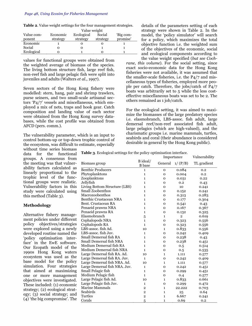
Page 48, Using Ecosim for Fisheries Management
values for functional groups were obtained from the weighted average of biomass of the species. The living bottom structure fish, large reef fish, non-reef fish and large pelagic fish were split into juveniles and adults (Walters et al., 1997). Seven sectors of the Hong Kong fishery were modelled: stern, hang, pair and shrimp trawlers, purse seiners, and two small-scale artisanal sec-tors ‘P4/7’ vessels and miscellaneous, which em-ployed a mix of nets, traps and hook gear. Catch composition and landing value of each sector were obtained from the Hong Kong survey data-bases, while the cost profile was obtained from AFCD (pers. comm.). The vulnerability parameter, which is an input to control bottom-up or top-down trophic control of the ecosystem, was difficult to estimate, especially without time series biomass data for the functional groups. A consensus from the meeting was that vulner-ability factors calculated as linearly proportional to the trophic level of the func-tional groups were realistic. Vulnerability factors in this study were calculated using this method (Table 3). Methodology Alternative fishery manage-ment policies under different policy objectives/strategies were explored using a newly developed routine named the ‘policy optimisation inter-face’ in the EwE software. Our Ecopath model of the 1990s Hong Kong waters ecosystem was used as the base model for the policy simulation. Four strategies that aimed at maximizing one or more management objectives were investigated. These included: (1) economic strategy; (2) ecological strat-egy; (3) social strategy; and (4) ‘the big compromise’. The
details of the parameters setting of each strategy were shown in Table 2. In the model, the ‘policy simulator’ will search for a policy, which maximizes the total objective function i.e. the weighted sum of the objectives of the economic, social and ecological components according to the value weight specified (but see Coch-
rane, this volume). For the social setting, since exact socio-economic data for the Hong Kong fisheries were not available, it was assumed that the smaller-scale fisheries, i.e. the P4/7 and mis-cellaneous types of fisheries, employed more peo-ple per catch. Therefore, the jobs/catch of P4/7 boats was arbitrarily set to 5 while the less cost-effective miscellaneous boats was set to be 2. The others remained as 1 job/catch. For the ecological setting, it was aimed to maxi-mize the biomasses of the large predatory species i.e. elasmobranch, LBS-assoc. fish adult, large demersal reef/non-reef associated fish adult, large pelagics (which are high-valued), and the charismatic groups i.e. marine mammals, turtles, seabirds and coral (their abundance is considered desirable in general by the Hong Kong public).
Table 3. Ecological settings for the policy optimisation interface. Importance Vulnerability
Biomass group B ideal/ B base
General 1/ (P/B) TL gradient
Benthic Producers 1 0 0.084 0.2 Phytoplanktons 1 0 0.004 0.2 Zooplanktons 1 0 0.031 0.22 Jellyfish 1 0 0.2 0.43 Living Bottom Structure (LBS) 1 0 10 0.241 Small Zoobenthos 1 0 0.152 0.241 Macrozoobenthos 1 0 0.313 0.283 Benthic Crustacean NRA 1 0 0.177 0.304 Bent. Crustacean RA 1 0 0.541 0.43 Penaeid prawns NRA 1 0 0.167 0.367 Penaeid prawns RA 1 0 0.132 0.325 Elasmobranch 5 1 2 0.619 Cephalopods NRA 1 0 0.323 0.556 Cephalopods RA 1 0 0.323 0.556 LBS-assoc. fish Ad. 10 1 0.833 0.556 LBS-assoc. fish Juv. 1 0 0.242 0.409 Small Demersal fish RA 1 0 0.238 0.43 Small Demersal fish NRA 1 0 0.238 0.451 Medium Demersal fish RA 1 0 0.5 0.514 Medium Demersal fish NRA 1 0 0.5 0.535 Large Demersal fish RA. Ad. 10 1 1.111 0.577 Large Demersal fish RA. Juv. 1 0 0.242 0.409 Large Demersal fish NRA. Ad. 10 1 1.111 0.577 Large Demersal fish NRA. Juv. 1 0 0.242 0.451 Small Pelagic fish 1 0 0.299 0.451 Medium Pelagic fish 1 0 0.4 0.577 Large Pelagic fish Ad. 10 1 0.833 0.661 Large Pelagic fish Juv. 1 0 0.299 0.472 Marine Mammals 2 1 22.222 0.703 Seabirds 2 1 25 0.64 Turtles 2 1 6.667 0.241 Corals 5 1 0.69 0.2
Table 2. Value weight settings for the four management strategies.
Value weight Value com-ponent
Economic strategy
Ecological strategy
Social strategy
‘Big com-promise’
Economic 1 0 0 1 Social 0 0 1 1 Ecological 0 1 0 1

Fisheries Centre/FAO Workshop, Page 49
Therefore, these groups were given higher values of B ideal/B base ratio and their importance was set as 1, while the others were set as 0. The B ideal/B base ratio was defined as the ratio of the user’s desired biomass to the biomass of that par-ticular functional group in the Ecopath base model. The ecological objective function was cal-culated from the B ideal/B base ratio, which was weighted according to the importance set. However, the relative ecological importance of particular functional groups in the model was highly subjective to the user. Therefore, the sug-gestion was made during the workshop that simu-lations should also be carried out under an im-portance setting which was equal to the reciprocal of the production/biomass ratio (P/B) in the base Ecopath model. It was generally a consensus at the workshop that low growth-rate, long-lived groups (low P/B ratio) are more vulnerable to ex-ploitation. Therefore the use of the reciprocal of P/B as the importance setting provided an objec-tive way to value ecological importance in the ecosystem during policy optimization. This ap-proach was adopted in our study. Simulations of a 30-year period were used to search for optimum fishing effort of the seven different fishery sectors under dif-ferent management. The resulting eco-nomical, social, and ecological objective functions, and fishing efforts were re-corded. Simulations were repeated for different starting fishing effort i.e. (1) Ecopath base F’s; (2) current F’s; and (3) random F’s, to ensure that a global opti-mum was obtained (F’s are the fishing ef-forts of the seven fishery sectors). In addi-tion, the trophic level of fishery catch (TLC) which resulted from the suggested fishing effort in each strategy was calcu-lated using:
TLC = [1/(Ct)] * Σ ( Ci* TLi),
Where, ΣCi = Ct, Ct is the total catch, while Ci is the catch by species i.
Sensitivity test Sensitivity of the policy simulations to different vulnerability settings was tested by repeating simulations under the four strategies with vulner-abilities of 0.2, 0.4, 0.6, and a gradient of vulner-abilities ranging from 0.2 to 0.7 which were di-rectly proportional to the trophic level of each functional group (Table 3). Moreover, sensitivity of the relative effect of the ecological stability on the economical and social performance was tested by running policy simula-tions under the settings in Table 4. Results Economic strategy Results from the policy simulation that aimed to maximize economic benefit from vulnerability settings of 0.4 and 0.6 generally suggest that fish-ing effort exerted by stern trawler (ST) should be increased by 0.5 to 1 times the Ecopath base value, while the other fishing sectors should be reduced or increased slightly (Figure 2). However, for a vulnerability setting of 0.2, the re-sult suggested effort increases in purse seine (PS) and small outboard engine boat (P4/7), with ef-fort decreased for stern trawlers and other fishing sectors. The results from vulnerabilities propor-tional to the trophic level of the functional groups is similar to the results from vulnerability settings of 0.4 and 0.6, except that it suggested a more than two-fold increase in the ‘miscellaneous’ sec-tor.
Table 4. The value weight settings for sensitivity test between different weight value in the ecological stabil-ity component. For the the ‘big compromise’ and the ‘economical versus ecological’ strategies, simulations were run with ecological stabilities listed.
Value weight Value com-ponent
The ‘big compromise’
Economical versus Ecological
Economic 1 1 Social 1 0 Ecological 1, 2, 3, 4 0.1, 1, 2, 4, 6, 8, 10, 12
Misc
PT PS
ST
P4/7 HTSHT
-200%
-100%
0%
100%
200%
300%
Cha
nge
from
Eco
path
Bas
e F'
s
0.20.40.6TL
Figure 2. Suggested change of fishing effort for different fishing sectors in the economic strategy simulation.

Page 50, Using Ecosim for Fisheries Management
Social strategy The policy simulation that aimed to maximize so-cial strategy suggested increases in fishing effort of pair trawl, purse seine, hang trawl and P4/7 sectors to maximize social benefits (jobs/catch) (Figure 3). However the suggested results were sensitive to the vulnerability setting.
Ecological stability strategy Results from the policy simulator sug-gested more than 50% decrease in ef-fort for all fishing sectors to maximize ecological stability (as defined in the B ideal/B base and importance settings). These are consistent between simu-lated results from different vulnerabil-ity settings (figure 4). The ‘big compromise’ Results from policy simulator that aimed to maximize all the objective functions (economical, social and eco-logical) over all the vulnerability set-ting (0.2, 0.4, 0.6 and proportional to trophic level) generally suggested that the P4/7 fishing boats should be in-creased by 0.5 to 2-fold, while the oth-
ers should be decreased slightly. Results from simulations of this strategy were generally consistent between different vulnerabilities except that it suggested shrimp trawl effort should increase more than 2-fold at a vulnerability of 0.2, while the others decrease in effort. Moreover, the amount of suggested effort increase in the P4/7 sector was greater at a higher vulnerability setting. When the vulnerability was set to be proportional to the trophic level of the functional group, and the reciprocal of the P/B ratio was used as ecological importance set-ting, the simulation results sug-gested higher increase in the P4/7 effort, and a general effort in-crease in other fishing sectors (Figure 5). The economical, social, and eco-logical objective functions (per-formance) of the four strategies are summarized in Table 5. Moreover, simulation with vary-
ing ecological value weight setting in different strategies showed that the economic and social performances correlated negatively with the in-creasing ecological stability setting (Figure 6). It was also found that the economic, social and eco-logical performance responded strongly with changing ecological stability setting when the eco-logical setting was increased from 0 to 2. When
Table 5. Performance of the economical, social, and ecological objective functions for the four strategies.
Strategy Strategy Economic Social Ecological Overall Economic 1 2574.6 15550.5 -10458.3 0.23 Ecological 2 487.2 1257.3 -7672.6 -1.46 Social 3 -25250.7 57572.6 -12935.2 3.47 ‘Big Compromise’ 4 1781.7 25020.2 -9966.7 -0.09
-1000%
0%
1000%
2000%
3000%
4000%
5000%
6000%
7000%
8000%
ST SHT PT PS P4/7 Misc HT
Cha
nge
in fi
shin
g ef
fort
0.20.40.6TL
Figure 3. Suggested change of fishing effort for different fishing sectors in the social strategy simulation.
PS
ST
PT
P4/7
MiscHT
SHT
-1.5
-1
-0.5
0
0.5
1
1.5
2
2.5
3
3.5
Cha
nge
from
Eco
path
bas
e F'
s
0.2
0.4
0.6
TL
1/ (P/B)
Figure 4. Suggested change of fishing effort for different fishing sectors in the ecological strategy simulation

Fisheries Centre/FAO Workshop, Page 51
the ecological setting was increased to more than two, changes of the three performances were much weaker. Trophic level of catch The mean trophic level of catch calculated from the four strategies (with vulnerability setting pro-portional to trophic level of the functional group) showed that strategy maximizing eco-logical stability resulted in the highest mean trophic level while the strategy maximizing so-cial benefits resulted in the lowest. Also, TLC lower than the base Ecopath value resulted from the economic strategy. The “big compro-mise” strategy produced an intermediate TLC among all strategies (Table 6).
Discussion Our results were con-sistent with general observations of fish-eries management. Simulation with ob-jective policy that maximizes economic performance favours rapid turnover lower trophic level species, while a higher tro-phic level of fishery catch is achieved when ecological goals favour larger preda-tors. Moreover, in-crease priority to
maximize ecological sta-bility resulted in de-creasing economic bene-fits. When the policy that maximizes jobs was prioritized, fisheries sec-tors that use more la-bour, typically small-scale mixed inshore fisheries were favoured. This is in parallel with the syndrome of Mal-thusian overfishing ob-served in developing countries (Pauly, 1997). The optimization proc-ess for each manage-ment objective function involves restarting using different parameter val-ues until no future im-
provement can be achieved. This proved to be much more difficult when higher values of vul-nerability were assumed (>0.5), this likely results from a more complex response surface with many local optima. Automation of this process will as-sist users. Other optimization processes that can find the global optima could be employed.
Table 6. Mean trophic level of catch resulting from the suggested fishing effort from simulation of the four strategies. Strategy
Trophic level of fishery catch
Base Ecopath model value 3.16 Economic only 3.14 Social only 2.45 Ecological only 3.40 The ‘big compromise’ 3.21
P S
S HT
HTM isc
P 4/7
P T
S T
-1.5
-1
-0.5
0
0.5
1
1.5
2
2.5
3
3.5
Chan
ge fr
om E
copa
th b
ase F
's
0.2
0.4
0.6
TL
1/ (P/B)
Figure 5. Suggested change of fishing effort for different fishing sectors for the ‘bigcompromise’ strategy at different vulnerability factor settings: 0.2, 0.4, 0.6,proportional to the trophic level (TL), and to the reciprocal of theproduction/biomass (P/B) ratio.
0
500
1,000
1,500
2,000
2,500
3,000
-11,000 -10,000 -9,000 -8,000 -7,000
Ecological performance
Econ
omic
per
form
ance
0
5,000
10,000
15,000
20,000
25,000
30,000So
cial
per
form
ance
EconSocialLinear (Social)Linear (Econ)
Figure 6. Plot of economic and social performance against ecological performance. The R-squares of the fitted line in the economic and social performance are 0.96 and 0.86 re-spectively.

Page 52, Using Ecosim for Fisheries Management
Moreover, we noted instability of the ecosystem at higher values of vulnerability. Since the model employed in this study was preliminary, we be-lieve that more stable ecosystem might result fine tuning the input parameters. During this workshop, there were numerous revi-sions to the software. For consistency we used the version available at the end of the workshop (19th July 2000 version). The impact of later versions on our findings is unknown, however, from the changes seen to interim results during the work-shop, we believe that they may be generally ro-bust. It was the consensus at the workshop that this approach shows real promise, and will gain credi-bility once the method is stable and well tested. It offers excellent insights into management trade-offs in an ecosystem context. References Agriculture and Fisheries Department 1996. Annual
Report. Hong Kong Government. Alino, P. M., L. T. McManus, J. W. McManus, C. L.
Nanola, M. D. Fortes, G. C. Trono, and G. S. Ja-cinto 1993. Initial parameter estimations of a coral reef flat ecosystem in Bolinao, Pangsinan, Northwestern Philippines. in V. Christensen and D. Pauly, editors. Trophic models of aquatic ecosystems. ICLARM Conf. Proc. 26.
Arreguin-Sanchez, F., J. C. Seijo and E. Valero-Pacheco 1993. An application of ECOPATH II to the north continental shelf ecosystem of Yucatan, Mexico. in V. Christensen and D. Pauly (eds) Trophic models of aquatic ecosystems. ICLARM Conf. Proc. 26.
Browder, J. A. 1993. A pilot model of the Gulf of Mex-ico continental shelf. in V. Christensen and D. Pauly, editors. Trophic models of aquatic ecosys-tems. ICLARM Conf. Proc. 26.
Buchary, E. A. 1999. Evaluating the effect of the 1980 trawl ban in the Java Sea, Indonesia: an ecosys-tem-based approach. M.Sc. University of British Columbia, Vancouver, Canada.
Cheung, K. 1965. Production and use of ice - Hong Kong. Pages 97-102 in Indo-Pacific fisheries council.
Cook, D. C., A. L. K. Chan, K. C. C. Fok, and K. D. P. Wilson. 1997. A fisheries resource profile prior to artificial reef deployment in Hong Kong. in PACON 97 symposium on resource development - environmental issues and the sustainable devel-opment of coastal waters, Hong Kong.
Dalsgaard, A. J. T. 1999. Modeling the Trophic Transfer of Beta Radioactivity in the Marine Food Web of Enewetak Atoll, Micronesia. M.Sc. Thesis. Uni-versity of British Columbia, Vancouver.
EVS 1996. Contaminated Mud Disposal at East Sha Chau: Comparative Integrated Risk Assessment. Prepared for Hong Kong Government, Civil Engi-neering Department.
Froese, R. and D. Pauly 1998. FishBase 98: Concepts Design and Data Sources. ICLARM, Manila.
Greze, V. N., and O. Kinne 1978. Production of animal population. in O. Kinne, editor. Marine Ecology: a Comprehensive, Integrated Treatise on Life in Oceans and Coastal Waters. Vol. 4. Dynamics. John Wiley & Sons, New York.
Hoyo, J. D., A. Elliott, J. Sargatal, and N. J. Collar 1992. Handbook of the birds of the world. Inter-national Council for Bird Preservation. Lynx Edi-cions, Barcelona.
Jarre-Teichmann, A., and D. Pauly 1993. Seasonal changes in the Peruvian upwelling ecosystem. in V. Christensen and D. Pauly, editors. Trophic models of aquatic ecosystems. ICLARM Conf. Proc. 26.
Morton, B. S. 1994. Hong Kong's coral communities: status, threats and management plans. Marine Pollution Bulletin 29:74-83.
Morton, B., and J. Morton 1993. The Sea Shore Ecology of Hong Kong. Hong Kong University Press, Hong Kong.
Ni, I. H., and K. Y. Kwok 1999. Marine fish fauna in Hong Kong waters. Zoological Studies 38:130-152.
Opitz, S. 1998. A quantitative model of the trophic in-teractions in a Caribbean coral reef ecosystem. Pages 259-268 in V. Christensen and D. Pauly, editors. Trophic models of aquatic ecosystems. ICLARM Conf. Proc. 26.
Palomares, M. L. D., and D. Pauly 1998. Predicting food consumption of fish populations as functions of mortality, food type, morphometrics, tempera-ture and salinity. Mar. Freshwater. Res. 49:447-453.
Pauly, D. 1997. Small-scale fisheries in the tropics: marginality, marginalization, and some implica-tions for fisheries management. Pages 1-9 in E. K. Pikitch, D. D. Huppert, and M. P. Sissenwine, edi-tors. Global trends: fisheries management.
Pauly, D., M. L. Soriano-Bartz, and M. L. D. Palomares 1993. Improved construction, parametrization and interpretation of steady-state ecosystem models. Pages 1-13 in V. Christensen and D. Pauly (eds) Trophic models of aquatic ecosystem. ICLARM Conf. Proc. 26.
Pauly, D., and V. Christensen 1995. Stratified models of large marine ecosystems: a general approach and an application to the South China Sea :148-174.
Pauly, D., V. Christensen and V.J. Sambilay 1990. Some features of fish food consumption estimates used by ecosystem modellers. ICES CM 1990/G 17:8pp.
Pitcher, T. J., R. Watson, A. Courtney, and D. Pauly 1998. Assessment of Hong Kong's inshore fishery resources. Fisheris Centre Research Reports 6(1): 155pp.
Pitcher, T.J., Watson, R., Haggan, N., Guénette, S., Kennish, R., Sumaila, R., Cook, D., Wilson, K. and Leung, A. (2000) Marine Reserves and the Restora-tion of Fisheries and Marine Ecosystems in the South China Sea. Bulletin of Marine Science 66(3): 530-566.
Polovina, J. J. 1984. Model of a coral reef ecosystem I. The ECOPATH model and its application to French Frigate Shoals. Coral Reefs 3:1-11.

Fisheries Centre/FAO Workshop, Page 53
Reilly, S. B., and J. Barlow 1986. Rates of increase in dolphin population size. Fishery Bulletin 84:527-533.
Sadovy, Y. 1998. Patterns of reproduction in marine fishes of Hong Kong and adjacent waters. Pages 261-273 in B. Morton, editor. The Third Interna-tional Conference on the Marine Biology of the South China Sea, Hong Kong. Hong Kong Univer-sity Press, Hong Kong.
Sadovy, Y. J., and A. S. Cornish 2000. Reef fishes of Hong Kong. Hong Kong University Press, Hong Kong.
Silvestre, G., S. Selvanathan, and A. H. M. Salleh 1993. Preliminary trophic model of the coastal fisheries resources of Brunei Darussalam, South China Sea. Pages 300-306 in V. Christensen and D. Pauly, editors. Trophic models of aquatic ecosystems. ICLARM Conf. Proc. 26.
Stather, K. 1975. The evolution of fishing craft in Hong Kong - 1947 to 1971. Hong Kong fisheries bulletin 2:1-9.
Trites, A. W., and D. Pauly 1998. Estimating mean body masses of marine mammals from maximum body lengths. Can. J. Zool. 76: 886-896.
Trites, A., and K. Heise. 1996. Marine Mammals. In D. Pauly and V. Christensen (eds) Mass-balance models of Northeastern Pacific ecosystem. Fisher-ies Centre Research Reports 4(1): 131 pp.
Trites, A. W., V. Christensen, and D. Pauly 1997. Com-petition between fisheries and marine mammals for prey and primary production in the Pacific Ocean. J. Northw. Atl. Fish. Sci. 22:173-187.
Wilson, K. D. P. 1997. The Hong Kong marine fish cul-ture industry - challenges for sustainable devel-opment. Proceedings of the first international symposium on marine conservation Hong Kong 1:86-97.
Walters, C., V. Christensen, and D. Pauly 1997. Struc-turing dynamic models of exploited ecosystem from trophic mass-balance assessment. Reviews in Fish Biology and Fisheries 7:139-172.

Page 54, Using Ecosim for Fisheries Management
Exploration of Management and Conservation Strategies for the Multispecies Fisheries of Lake Malawi using an Ecosystem Modelling Approach Edward Nsiku Fisheries Centre, UBC 2 Abstract Lake Malawi, one the African Great Lakes, is the most species-rich freshwater body in the world. Conserva-tion of the lake is thus one of the important areas that needs to be focused by the riparian countries bordering it as well as the scientific community and international funding agencies. The lake’s ecosystem and fish re-sources, which are some of the important factors in the implementation of conservation initiatives, are ana-lyzed through construction of an Ecopath model. Ap-plication of Ecosim routine follows in order to optimize policy, particularly of fisheries, in the objectives of maximizing fisheries rent, social benefits, rebuilding of mandated species and ecosystem structure or health. Trophic interrelationships in the functional groups, which include the main fish species caught, and trophic structure of the lake are assessed. Twenty-six func-tional groups are quantified. Chaoborus edulis, En-graulicypris sardella larvae and the predatory zoo-plankton, Mesocyclops aequatorialis aequatorialis, form the main pathway through which energy flows from bottom to top trophic levels in the Lake Malawi ecosystem. The trophic structure of the lake system de-teriorates over time. Maturity of the lake ecosystem is in the middle stages. Standing biomass and production rates, i.e. model control regimes, are dependent more on food availability rather than impact of predation. The model supports observations of overexploitation in most fish resources that form the main fisheries in Lake Malawi. This includes even offshore species, espe-cially those that are also exploited by traditional fishers such as kampango. The traditional fisheries sector con-tributes more than the commercial sector to the influ-ence fisheries has on the ecosystem of the lake. The analysis optimizes the exploitation and conservation goals for the ecosystem and fish resources of Lake Ma-lawi at reduced fishing effort and catch from the cur-rent levels. Introduction Lake Malawi is the third largest and second deep-est freshwater body in Africa. It is found at the southern tip of the East African Rift Valley. Its ri-parian countries are Malawi, Mozambique and Tanzania. The lake has a total surface area of 28800 km2 and an average depth of 292 m, with a
2 Current address: 109-7341 19th Avenue, Burnaby BC, Canada V3N 1E3; E-mail: [email protected].
maximum point of about 700 m. It also contains 7 % of the world’s total surface fresh water (Patter-son and Kachinjika 1995). Lake Malawi is among lakes with the most abundant fish species in the world (Barel et al. 1985; Ribbink 1991; Pitcher 1994). However, clear waters of low biological productivity characterize a large part of the lake (ICLARM/GTZ 1991). The southern part is shal-low and produces a lot of fish food and forms a rich-fishing area. There is an annual cycle of stratification during which epi-, meta- and hypo-limnion zones are marked from December to March. Mixing occurs from May to August. Depth, temperature and wa-ter currents cause these events. The first layer ex-tends from surface of the lake to 125 m in depth. The middle layer can be as deep as 230m. Beyond this is a third layer, which is permanently strati-fied and anoxic so that no mixing ever takes place. The effect of temperature in the water column is marked, with the presence of a sudden transition depth range, the thermocline, between 40 and 60m in January, and extending to 100m by May. The thermocline disappears during the cold 'mwera' season. Wind causes strong currents so that interchange of conditions and other proper-ties in the two upper layers, occur. Complete nu-trient mixing, therefore takes place only in the two zones. The euphotic zone, i.e. that part of the water column in which photosynthesis occurs, ex-tends to 70m. This is not affected by mixing in the upper two zones. Temperature drops as depth in-creases from the lake surface. As a result, the depth or temperature dependent chemical ele-ments including nutrients also vary (Beadle 1974; Eccles 1978; FAO 1993; Patterson and Kachinjika 1995; Patterson et al. 1995). Mixing of nutrient-rich deep waters and nutrient poor surface waters is vital for sustenance of the fisheries in the lake (Arnell et al. 1996; WWF 1999). The aim of this paper is to identify optimal poli-cies for exploiting and conserving the fish re-sources and ecosystem of Lake Malawi. The opti-mization is based on the basic estimates of an ecosystem model of the lake between 1976 and 1996 (Nsiku 1999). The focus is, however, on eco-system simulation (Walters et al. 1997; Christen-sen et al. 2000). The fisheries are optimized in re-lation to the management goals of maximizing rent, social benefits, rebuilding of mandated spe-cies, ecosystem structure and balancing all the goals. The analysis focuses on traditional and commer-cial fisheries sectors. These are the main sectors in the lake's fisheries apart from a minor contri-bution, in terms of catch amount, of the aquarium

Fisheries Centre/FAO Workshop, Page 55
or ornamental fisheries sector. The traditional fisheries sector is, however, the most important with respect to management concerns. Methods The trophic structure of the Lake Malawi ecosys-tem between 1977 and 1996 is constructed using Ecopath (Christensen and Pauly 1992) and eco-system simulation is run for a period of twenty years using Ecosim (Walters et al. 1997; Christen-sen et al. 2000). A mixed control regime is used in the simulation. The Ecopath input data are from research studies on Lake Malawi. Four studies contribute most of the data. They are the FAO programme between 1977 and 1981; Malawi Government, UNDP and FAO joint study from 1988 to 1992; ODA-UK/SADC project between 1990 and 1994; and ICEIDA research programme from June 1994 to March 1996 (Degnbol 1993; FAO 1993; Menz 1995; Banda and Tomasson 1997). Many other sources are also used. However, data for some of the trophic boxes are estimated in the model.
Diet compositions (Table 1) are from Nsiku (1999). In the present analysis the diets are edited a little for the lower groups. The model is set to represent the whole lake as one ecosystem. It has twenty-six functional groups (Table 2). There are nineteen fish groups and single trophic boxes for usipa larvae, phyto-plankton, molluscs, apex predators (fish eating avian, reptiles and mammals), zooplankton (her-bivorous and other species), detritus and lakefly. The model groups, especially those for fish, are identified by their Malawian vernacular names re-flective of indigenous technical knowledge (Berlin 1992), particularly of the fishing community's perception of similarities in the fish resources. The grouping is also guided by the system defini-tion, i.e., a functional group may be of ecologically or taxonomically related species, single species, or size/age items (Christensen and Pauly 1992). A strategy of varying fishing efforts over a twenty-year period at equilibrium biomass is first consid-ered. Vulnerability is set at 0.25. Secondly, the ef-
Table 1. Diet Composition for the Lake Malawi Ecopath model functional groups: 1977-1996 (values are rounded to two decimal places).
Prey\Predator
Nku
nga
Kam
pan
go
Mat
emba
Uta
ka
Nd
un
du
ma
Kam
buzi
Ch
isaw
asaw
a
Ch
ambo
Ch
ilu
ngu
ni
Mbu
na
Mch
eni
Bom
be
Mla
mba
Usi
pa
Usi
pa
larv
ae
San
jika
Mp
asa
Nch
ila
Nkh
olok
olo
Sam
wam
owa
Nkh
un
gu
Nkh
ono
Top
pre
d
Zoo
pla
nkt
on
Nkunga 0.01
Kampango 0.01
Matemba 0.05
Utaka 0.01 0.01 0.01 0.01 0.01 0.01
Ndunduma 0.09 0.01 0.01 0.01 0.12 0.01 0.10
Kambuzi 0.02 0.06 0.01 0.01 0.01
Chisawasawa 0.01 0.01 0.01 0.01
Chambo 0.01 0.01 0.01
Chilunguni 0.01 0.01 0.01
Mbuna 0.16 0.3 0.07 0.30 0.15 0.05 0.20
Mcheni 0.02
Bombe 0.01 0.05
Mlamba 0.01 0.01 0.05
Usipa 0.05 0.25 0.01 0.28 0.20 0.20
Usipa larvae 0.01 0.04 0.10 0.05 0.52 0.05 0.38 0.38
Sanjika
Mpasa
Nchila
Nkholokolo 0.02
Samwamowa 0.01 0.01
Nkhungu 0.09 0.22 0.45 0.05 0.07 0.09 0.05 0.03 0.12 0.3 0.3 0.59 0.02
Nkhono 0.09 0.06 0.02 0.09 0.10 0.01 0.05 0.01 0.15 0.01 0.18
Top predators 0.10
Zooplankton 0.18 0.20 0.09 0.11 0.12 0.09 0.02 0.20 0.05 0.09 0.02 0.5 0.53 0.1 0.09 0.01 0.12 0.15 0.53 0.01
Phytoplankton 0.36 0.48 0.17 0.71 0.67 0.90 0.90 0.47 0.04 0.25 0.15 0.45 0.51 0.08 0.27 0.47 0.15 0.90
Detritus 0.01 0.02 0.05 0.01 0.01 0.08 0.05 0.02 0.30 0.17 0.01 0.15 0.20
Import 0.67 0.24 0.15 0.02 0.20 0.05 0.05 0.01 0.15 0.46 0.02 0.23 0.02 0.02 0.03 0.30 0.05 0.25 0.01 0.65 0.28 0.09
Sum 1.00 1.00 1.00 1.00 1.00 1.00 1.00 1.00 1.00 1.00 1.00 1.00 1.00 1.00 1.00 1.00 1.00 1.00 1.00 1.00 1.00 1.00 1.00 1.00

Page 56, Using Ecosim for Fisheries Management
fect of different management goals on traditional and commercial fisheries sectors is analyzed. This part covers five management goals (Table 3). The traditional and commercial fisheries sectors are applied as fleets with jobs/catch value of 0.741 and 0.259 respectively. These are based on the to-tal catches rather than values of the sectors in Ta-ble 4. Input fleet costs used in the model fishery simula-tion are in Table 5. The mandated rebuilding fo-cuses on seven species-based fisheries (Table 6). One modification is made for analysis of fisheries sector landings. The catch, which is based on the
traditional fisheries, is taken to represent total catch from Lake Malawi. Proportions of tradi-tional and commercial fisheries to the total catch are based on Turner (1977), Tweddle and Magasa (1989), Pitcher (1994), Turner (1995, 1996), Banda et al. (1996), and Banda and Tomasson (1997) for the different species-based fisheries (Table 4). Results Table 7 details the basic estimates of the model. The model is also graphically summarized in Fig-ure 1. Many groups in lower trophic boxes utilize
Table 2. Summary of the Lake Malawi ecosystem model functional groups. # Local Name Details1 1 Nkunga Eel Anguilla nebulosa and mastacembelids Mastacembelus shiranus and M. sp. 'Rosette' 2 Kampango Bagrid catfish Bagrus meridionalis. 3 Matemba Represents barbel cyprinids, one alestiid, two cyprinodontids and one anabantid. 4 Utaka Bottom feeding cichlids in genera Copadichromis, Cyrtocara, Maravichromis and Nyas-
sachromis. 5 Ndunduma Demersal and off-shore cichlids belonging to genera Diplotaxodon, Palladichromis and
Placidochromis. 6 Kambuzi Cichlids in genera Protomelas, Hemitaeniochromis Dimidiochromis, and Taeniochromis 7 Chisawasawa Mostly bottom feeding cichlids in genera Lethrinops, Taeniolethrinops and Tramiti-
chromis. 8 Chambo Refers to three species of pelagic tilapiine cichlids in the genus Oreochromis; O.
squampinis, O. lidole and O. karongae. 9 Chilunguni Two cichlid species, Tilapia rendalli and Oreochromis shiranus are specified in this
group. 10 Mbuna Rock-dwelling cichlids popular with tropical fish aquarists and ornamental tropical fish
trade. Most species belong to genus Pseudotropheus. There are thirteen other mbuna gen-era2.
11 Mcheni Are offshore, pelagic and demersal occurring tigerfish cichlids in the genus Rampho-chromis.
12 Bombe Ten species of large clariid catfishes in the genus Bathyclarias. 13 Mlamba Clariid catfishes in the genus Clarias. There are four species; C. gariepinus, C. mellandi,
C. mossambicus and C. theodorae. 14 Usipa Refers to the cyprinid Engraulicypris sardella. 15 Usipa larvae Larvae stage of Engraulicypris sardella. 16 Sanjika Refers to bariliine cyprinid Opsaridium microcephalus 17 Mpasa The bariliine cyprinid Opsaridium microlepis. 18 Nchila Represents two cyprinids, Labeo mesops and L. cylindricus. Only L. mesops supports a
fishery in the lake. 19 Nkholokolo Refers to squeakers: two small mochokids Synodontis njassae and Chiloglanis neumanni.
The main species, S. njassae, is endemic to the lake. 20 Samwamowa Represents mormyrid species in the genera of Marcusensis, Mormyrus and Petrocepha-
lus. 21 Nkhungu The lakefly Chaoborus edulis forms a key link in energy flow in the lake ecosystem. 22 Nkhono The group represents gastropod and lamellibranch molluscs. 23 Top predators This group represents higher animals; fish-eating birds, reptiles (monitor lizards and
crocodiles) and otters. 24 Zooplankton The group has herbivorous and carnivorous zooplankton which include copepods (Meso-
cyclops aequatorialis aequatorialis, Tropodiaptomus canningtoni, and Thermocyclops neglectus), cladocerans (Diaphonosoma excisum and Bosmina longrostris), naupulii, Diaptomus kraepelini and Mesocyclops leuckarti.
25 Phytoplankton This functional group includes species in the genera Aulacoseira, Surirella, Stephanodis-cus, Mougeotia, Cymatopleura, Closterium, Synedra and Staurastrum.
26 Detritus Represents organic matter, either dissolved or particulate.
1. A detailed list of fish species in Lake Malawi is found in Nsiku (1999). 2. They are Cyathochromis, Cynotilapia, Docimodus, Electochochromis, Exochromis, Fossorochromis, Genyochromis, Gephro-chromis, Hemitilapia, Iodotropheus, Melanochromis, Nimbochromis, and Petrotilapia. However, some of the mbuna genera are being revised (Snoeks 2000).

Fisheries Centre/FAO Workshop, Page 57
detritus apart from phytoplankton. The ecotro-phic efficiencies are in the range of 0.10 - 0.95 ex-cept for nkholokolo and detritus both of which have an EE value of 0.007. It is not clear whether this is only due to low predation exerted on the groups. Almost all the production over consump-tion ratio values or gross food conversion effi-ciencies (GE) fall in the expected range of 0.1 - 0.3 (Christensen and Pauly 1992). Two exceptions are the values of nkholokolo and top predators at 0.059 and 0.435 respectively. Groups with GE values close to 0.3 include matemba, bombe, usipa and nkhungu. Among these functional groups only bombe has relatively large-sized species. With the exception of usipa larvae which has an R/B value of 458.0 year-1, the respiration over biomass ratios, which can be any positive value (Christensen and Pauly 1992), are in the normal range of 0-100 (Bundy 1998). Overall, the value of production over consump-tion ratio is 0.0005. Therefore, Lake Malawi sys-tem has very low gross efficiency, i.e. limited
quantities of discrete trophic flows (Christensen and Pauly 1992; Dalsgaard 1999). The lake system fishery has a mean trophic level of 3.7. The bio-mass over total throughput is 0.008 year-1 and omnivory index is 0.426. The production over respiration ratio (P/R) is at 2.95, less than the value of 5.88 given in Nsiku (1999). In the mixed trophic impact (MTI) analysis of the Lake Malawi ecosystem, phytoplankton and, to a lesser extent detritus have greatest influence and are the basis of energy flow in the lake. Lower groups that have positive impact are nkhungu Chaoborus edulis, usipa larvae and zooplankton. The MTI and graph of model trophic structure support observations of Allison et al. (1995a) that lakefly, larvae of E. sardella and predatory zoo-plankton Mesocyclops aequatorialis aequatori-alis are the main users of secondary production in the Lake Malawi ecosystem. Fish groups that con-tribute most to the lake system are usipa and mbuna.
Table 3. Specifications of the management goals utilized for the optimization of the fisheries in Lake Malawi at vul-nerabilities (V) 0.2, 0.27a, 0.5 and 0.7. Weights assigned to performance indicators Management goal
Symbol Net economic value
Social (employment) value
Mandated re-building
Ecosystem structure
Optimizing net economic value MS1 1.0000 0.0001 0.0001 0.0001 Optimizing social (employment) value MS2 0.0001 1.0000 0.0001 0.0001 Optimizing mandated rebuilding MS3 0.0001 0.0001 1.0000 0.0001 Optimizing ecosystem structure MS4 0.0001 0.0001 0.0001 1.0000 Optimizing all goals MS5 1.0000 1.0000 1.0000 1.0000
Table 4. Catch contributions a of the traditional and commercial fleets derived from the 1976-96 mean catch of the traditional fisheries in Lake Malawi (values are based on prices of 1996; dash indicates insignificant amount; figures are rounded to two decimal places).
Fish Group Fleetb Catch Value Pricec
Total Traditional Commercial Total Traditional Commercial (MWK/Kg) (t) (t·km-2) (t·km-2) (t·km-2) (MWK'106) (MWK'106) (MWK'106)
Chambo 4398 0.15 0.10 0.06 62.63 39.85 22.77 14.24 Chilunguni 356 0.01 0.01 0.00 3.58 3.58 0.00 10.05 Kambuzi 2224 0.08 0.08 0.00 11.36 11.36 0.00 5.11 Utaka 10271 0.36 0.22 0.14 62.55 38.49 24.06 6.09 Chisawasawa 179 0.01 0.00 0.01 1.33 0.00 1.33 7.41 Kampango 2005 0.07 0.04 0.03 17.96 10.78 7.19 8.96 Mcheni 259 0.01 0.01 0.00 2.00 2.00 0.00 7.72 Mlamba 1533 0.05 0.04 0.01 12.75 9.57 3.19 8.32 Usipa 5858 0.20 0.16 0.04 41.71 33.37 8.34 7.12 Nchila 168 0.01 0.01 0.00 1.96 1.96 0.00 11.67 Mpasa 112 0.00 0.00 0.00 1.66 1.66 0.00 14.82 Sanjika 122 0.00 0.00 0.00 1.15 1.15 0.00 9.39 Ndunduma 146 0.01 0.00 0.01 1.83 0.00 1.83 12.56 Bombe 1465 0.05 0.04 0.01 12.19 9.14 3.05 8.32 Nkholokolo 37 0.00 0.00 0.00 0.29 0.29 0.00 7.72 Mean 1942 0.07 0.05 0.02 15.66 10.88 4.78 9.30 Total 29133 1.01 0.71 0.30 234.95 163.19 71.76 139.50
Source for catch: MDF (1996). aThe proportions of the catches in the sectors are scaled to equal 1 before the amounts are rounded off to two decimal places, i. e., fleet jobs/catch value of 0.741 for traditional and 0.259 for commercial fisheries; bFleet in this analysis designates a fisheries sector comprising of many fishing units, sometimes of different fishing gears; cThis is beach or landing price; rate of exchange for 1US$ = 15.3 MWK in 1996 (IMF 1998).

Page 58, Using Ecosim for Fisheries Management
A limited positive impact is from ndunduma and utaka with much less contribution from chambo and kambuzi. With the exception of bombe, terti-ary consumers with trophic levels of 3.4 and above which also include nkunga, kampango, san-jika, mpasa, mcheni and top predators do not have any positive impact in the lake (Figure 2a). Each group's contribution to the lake system is indicated by its sum of the mixed trophic impacts (Figure 2b). Apart from nchila and matemba, which have neither positive nor negative total im-pacting effect but are marginally impacted by the lake system, both chambo's impacted and impact-ing total values are the least. Nkhono is the only group with negative total values in its impacted and impacting effect.
Figure 3 summarizes the effect of changing fishing effort on equilibrium biomass for the Lake Malawi ecosystem. Simulation of fisher-ies of the lake as a whole is achieved by run-ning the combined fleet option. Vulnerabili-ties that result in smooth model runs for the equilibrium biomass analysis are between 0.10 and 0.29. A fishing rate of 1.0 does not vary biomass in the functional groups. Bio-mass decreases in almost all fish groups that support fishing operations as fishing rate
rises. The groups most affected are chambo, mpasa, kampango, utaka, sanjika, nchila and
Table 6. Ratios of the fishery groups focused upon for the mandated rebuilding management goal; values for the analysis are specified for mandated relative bio-mass and are default for structure relative weight.
No.
Group
Mandated Relative Biomass
Structure Rela-tive Weight
1 Kampango 1.0 1.2 2 Utaka 1.0 2.0 3 Kambuzi 1.0 2.0 4 Chambo 1.0 2.0 5 Sanjika 1.0 1.6 6 Mpasa 1.0 1.6 7 Nchila 1.0 0.2
Table 5. Some economic factors for Lake Malawi's traditional and commercial fisheries sectors.
Fishery
Fixed cost (%)
Effort re-lated to cost (%)
Sailing related
cost (%)
Profit
(%)
Total value (%)
Traditional 0.00 21.20 1.00 77.80 100 Commercial 30.90 21.40 25.60 22.10 100 Mean 15.45 21.30 13.30 49.95 100
Data sources used for estimates: ICLARM/GTZ 1991; GOM/UN 1992; GOM 1997.
Table 7. Basic estimate parameters for the Lake Malawi ecosystem between 1977 and 1996 (estimated Ecopath model parameters are in italics/light shading. Dashes mean that data cannot be assigned or is not available; most values are rounded to two decimal places). Data sources are given in Nsiku (1999).
Nu
mbe
r
Gro
up
Nam
e
Tro
ph
ic le
vel
Bio
mas
s (t
·km
-2)
Pro
du
ctio
n o
ver
biom
ass
(yea
r-1 )
Con
sum
pti
on
over
bio
mas
s (y
ear-
1 )
Eco
trop
hic
eff
i-ci
ency
Pro
du
ctio
n o
ver
con
sum
pti
on
Cat
ch
(t·k
m-2
·yea
r-1 )
Flo
w t
o d
etri
tus
(t·k
m-2
·yea
r-1 )
Net
eff
icie
ncy
Om
niv
ory
ind
ex
Res
pir
atio
n
(t·k
m-2
·yea
r-1 )
Ass
imil
atio
n
(t·k
m-2
·yea
r-1 )
Pro
du
ctio
n o
ver
resp
irat
ion
Res
pir
atio
n o
ver
biom
ass
(yea
r-1 )
1 Nkunga 3.4 0.00 0.80 4.00 0.94 0.20 – 0.00 0.25 0.99 0.00 0.00 0.33 2.402 Kampango 3.7 0.28 0.90 5.45 0.34 0.17 0.07 0.47 0.21 0.45 0.97 1.22 0.26 3.463 Matemba 2.7 0.00 4.60 11.05 0.87 0.30 – 0.00 20.52 0.68 0.00 0.01 1.09 4.244 Utaka 2.6 1.98 0.50 5.67 0.48 0.09 0.36 2.77 0.11 0.49 8.01 9.00 0.12 4.045 Ndunduma 3.2 2.49 0.50 5.87 0.76 0.09 0.01 3.23 0.11 0.48 10.45 11.69 0.12 4.206 Kambuzi 2.2 0.49 0.50 3.90 0.95 0.13 0.08 0.39 0.16 0.19 1.27 1.52 0.19 2.627 Chisawasawa 2.3 0.31 0.50 5.06 0.67 0.10 0.01 0.37 0.12 0.29 1.11 1.27 0.14 3.558 Chambo 2.1 0.57 0.50 5.06 0.81 0.10 0.15 0.63 0.12 0.07 2.02 2.30 0.14 3.559 Chilunguni 2.0 0.27 0.50 4.48 0.67 0.11 0.01 0.28 0.14 0.01 0.08 0.96 0.16 3.0810 Mbuna 2.5 7.47 0.50 5.06 0.67 0.10 – 8.79 0.12 0.45 26.49 30.23 0.14 3.5511 Mcheni 3.5 0.29 0.50 5.39 0.28 0.09 0.01 0.41 0.12 0.17 1.09 1.23 0.13 3.8112 Bombe 3.4 1.11 0.90 3.31 0.09 0.27 0.05 1.64 0.34 0.78 1.94 2.94 0.52 1.7513 Mlamba 2.7 1.16 0.90 5.33 0.15 0.17 0.05 2.13 0.21 0.78 3.91 4.96 0.27 3.3614 Usipa 2.9 0.56 2.50 9.23 0.76 0.27 0.20 1.36 0.34 0.31 2.73 4.13 0.51 4.8815 Usipa larvae 2.5 0.13 62.00 650.00 0.61 0.10 – 20.07 0.12 0.22 59.54 67.60 0.14 458.0016 Sanjika 3.6 0.03 0.60 6.21 0.22 0.10 0.00 0.05 0.12 0.07 0.13 0.15 0.14 4.3717 Mpasa 3.6 0.02 0.60 4.23 0.33 0.14 0.00 0.03 0.18 0.07 0.06 0.07 0.22 2.7818 Nchila 2.0 0.01 4.00 40.00 0.15 0.10 0.01 0.11 0.13 0.09 0.28 0.32 0.14 28.0019 Nkholokolo 3.2 0.59 0.50 8.50 0.01 0.06 0.00 1.30 0.07 0.24 3.72 4.01 0.08 6.3020 Samwamowa 2.6 0.00 1.95 11.62 0.36 0.17 – 0.00 0.21 0.70 0.01 0.01 0.27 7.3521 Nkhungu 2.5 1.75 19.40 69.70 0.47 0.28 – 42.39 0.35 0.21 63.62 97.58 0.53 36.3622 Nkhono 2.0 5.00 0.42 5.60 0.95 0.08 – 5.71 0.09 0.15 20.29 22.40 0.10 4.0623 Top predators 3.6 0.00 25.22 58.00 0.23 0.44 – 0.03 0.54 0.73 0.02 0.05 1.19 21.1824 Zooplankton 2.0 5.38 30.50 144.57 0.93 0.21 – 167.79 0.26 0.03 458.14 622.23 0.36 85.1625 Phytoplankton 1.0 7.62 258.40 – 0.36 – – 1257.14 – 0.00 0.00 – – –26 Detritus 1.0 – – – 0.01 – – 0.00 – 0.25 0.00 – – –

Fisheries Centre/FAO Workshop, Page 59
kambuzi. A limited drop in biomass is also ob-served in usipa, chilunguni and bombe. However only two fish groups; nkholokolo and ndunduma gain some biomasses. Mcheni, chisawasawa and mlamba are not affected by a change in the fish-ing rate. There is a reversal in trends when the fishing rate decreases. Lower groups of usipa larvae, zooplankton and phytoplankton as well as the functional groups that do not currently support active fisheries are not directly affected by varying fishing rates. The only linked group of juveniles and adults in the model, usipa and its larvae, does not produce any smooth simulated pattern. The linkage is thus not effected in the present simulation of Lake Malawi ecosystem. The effect of varying fishing rate in the tradi-tional and commercial fisheries sectors is in gen-eral similar to that observed in Fig. 3. Positions of fish groups, with respect to extent of changes in biomass, are however different. In the tradi-tional fisheries groups, which have the worst bio-mass reduction, we find mpasa, chambo, kampango, sanjika, kambuzi, utaka and nchila. There is a biomass increase in ndunduma. Bio-mass gain is only barely perceptible in nkholokolo and chisawasawa. The ratio of bio-mass over original biomass is close to unity in bombe and mlamba. Fish groups with a marginal
Figure 1. Graphic summarization of the Lake Malawi ecosystem trophic structure between 1977 and 1996.
Figure 2a. Mixed trophic impact of the Lake Malawi ecosystem be-tween 1977 and 1996.

Page 60, Using Ecosim for Fisheries Management
decrease in biomass are similar to those in the combined fleet option. For the commercial fisher-ies decrease in biomass occurs in chambo, utaka, kampango and, to a very limited extent, chisawa-sawa. Kambuzi gains a little biomass. The ratio of biomass over original biomass is almost constant in bombe, mlamba, ndunduma and usipa. Figure 4 shows the optimized ‘end over starting effort’ (E/S) ratios for the management goals in the model fishing policy searches. Optimization of fisheries decreases effort in the man-agement goals. There are, however, a number of in-stances that opti-mize specific fish-ing policy objectives at efforts above the base levels. These occur in all the management goals except for that of optimizing man-dated rebuilding of species (MS3). For the management goal of optimizing economic value (MS1), effort above the base level oc-
curs in the category of the traditional fisheries at all vulnerabilities. In the management goal of op-timizing social (employment) value (MS2), com-mercial fisheries category has two outlier E/S ef-fort ratios of 20.37 and 20.09 at vulnerability lev-els of 0.7 and 0.5 respectively. These are omitted from Figure 4b. Other efforts exceeding the starting levels are in traditional fisheries category at all vulnerabilities as well as in categories of total and social values
-1.15
-0.50
0.15
0.80
1.45
Nku
nga
Kam
pang
o
Mat
emba
Uta
ka
Ndu
ndum
a
Kam
buzi
Chi
saw
asaw
a
Cha
mbo
Chi
lung
uni
Mbu
na
Mch
eni
Bom
be
Mla
mba
Usi
pa
Usi
pa la
rvae
Sanj
ika
Mpa
sa
Nch
ila
Nkh
olok
olo
Sam
wam
owa
Nkh
ungu
Nkh
ono
Top
pred
ator
s
Zoop
lank
ton
Phyt
opla
nkto
n
Det
ritus
Fish
ery
Imp act ing Imp act ed
Figure 2b. Mixed trophic impacts summed up for each functional group in the Lake Malawi ecosystem; impacting value of phytoplankton is 9.23, it is not fully shown in the graph.
Figure 3. Trends of the ratios of biomass over starting biomass in the species-based fisher-ies in Lake Malawi when fishing rate varies over a twenty-year simulation period while ap-plying a mixed control regime or vulnerability of 0.25 for model equilibrium biomass simu-lation.

Fisheries Centre/FAO Workshop, Page 61
at vulnerability 0.7. The only negative E/S effort ratio value of -0.84 also occurs in MS2 for the economic category at vulnerability 0.5. In MS3 decreased effort ratios are in categories of eco-nomic and social values while in the rest they are almost unity. The management goal of optimizing ecosystem structure (MS4) generates effort levels that increase with vulnerabilities for ecosystem structure and total value categories. The E/S effort ratios for MS4's mandated rebuild-ing category remain at unity. In the remaining op-timized categories of MS4, effort decreases at all vulnerabilities. The heaviest drop is in traditional fisheries category. The management goal of opti-mizing all objectives (MS5) has above base effort in traditional fisheries category at vulnerabilities 0.2 and 0.27 as well as ecosystem structure cate-gory for vulnerability levels of 0.5 and 0.7. If equi-librium biomass vulnerabilities (i.e., with maxi-mum of 0.29) are taken into account, only vul-nerabilities of 0.2 and 0.27 may be focused on. In
this case E/S effort ratios above unity fall in the 1.086 - 3.093 range and are obtained in the tradi-tional fisheries category for MS1, MS2 and MS5. For MS4 they are in the total value and ecosystem structure categories. Figure 5 shows catch trends for the traditional and commercial fisheries in all the management goals. The traditional fisheries catch ratios have similar trends to those of total fisheries for almost all cases. E/S catch ratios in the management goals are either unity or less except in MS4 (Fig. 5d). In MS1 catch ratios increase for the tradi-tional fisheries as the vulnerabilities rise. The commercial fisheries' catch ratios decrease at vul-nerabilities between 0.2 and 0.27 and rise again through to vulnerability 0.7. The catch ratios in MS2 are lowest at vulnerability 0.5. In MS3 the E/S catch ratios are unity at vul-nerabilities 0.2 and 0.27 but they are lower at
0.0
0.5
1.0
1.5
2.0
TV EV SV MR ES TF CFOpt imized catego ry
MS5V0.20 MS5V0.27 MS5V0.50 MS5V0.70Fig. 4e
0.0
0.5
1.0
1.5
2.0
2.5
TV EV SV MR ES TF CFOptimized catego ry
MS1V0.20 MS1V0.27 MS1V0.50 MS1V0.70
Fig. 4a
0.0
0.5
1.0
1.5
2.0
2.5
TV EV SV MR ES TF CFOptimized catego ry
MS1V0.20 MS1V0.27 MS1V0.50 MS1V0.70
Fig. 4a
0.0
0.5
1.0
1.5
2.0
2.5
TV EV SV MR ES TF CFOptimized catego ry
MS1V0.20 MS1V0.27 MS1V0.50 MS1V0.70
Fig. 4a
0.0
0.5
1.0
1.5
2.0
2.5
TV EV SV MR ES TF CFOptimized catego ry
MS1V0.20 MS1V0.27 MS1V0.50 MS1V0.70
Fig. 4a
Figure 4. E/S effort ratios simulated for the different vulnerabilities in the management goals of optimizing economic value (MS1, 4a); social (employment) value (MS2, 4b); mandated rebuilding of species (MS3, 4c); ecosystem structure (MS4, 4d);and all objectives (MS5, 4e). The optimized categories in each management goal is represented by abbreviations TV for total value, EV for economic value, SV for social value, MR for mandated rebuilding, ES for ecosystem structure, TF for traditional fisheries, and CF for commercial fisheries.

Page 62, Using Ecosim for Fisheries Management
vulnerabilities 0.5 and 0.7. In MS4 and MS5 commercial fisheries obtain higher E/S catch ra-tios than traditional or total fisheries at all vul-nerability levels. The fisheries simulated values mirror trends of the catches. At 1996 prices, Lake Malawi fisheries obtain in Malawi kwacha per tonne (MWK/t) a total value or market value of 8204.48; total fixed cost of 689.9; total variable cost of 2375.1; total cost of 3065.01; and profit of 5139.47. Considering that only the traditional fisheries catch has been used as input for model simulation, the summary values fall short of ac-tual values by at least 15 %, which is the average contribution of the commercial fisheries to the lake's total landings. The cost does not change in commercial fisheries for all management goals. Traditional fisheries do not generate any costs probably due to nil fixed cost entry in Table 5. Table 8 details the values of performance indica-tors at all vulnerability levels in the management strategies for both open and close loop model simulations. Within performance indicators
higher values are in general optimized at lower vulnerability values. Each management goal op-timizes fisheries in its own performance indica-tor, for example, MS1 generates highest values in economic value indicator at all vulnerability lev-els. However, at vulnerability 0.5, the economic indicator is optimized in MS2 instead of in MS1. Optimized indicator values are higher in open loop than in closed loop simulations. There are a few exceptions, though. The close loop has higher indicator values for mandated rebuilding and ecosystem structure in MS2 at vulnerability 0.27. The same occurs at a vulnerability of 0.7 for man-dated rebuilding indicator in MS4. Values of per-formance indicators are similar, again, for man-dated rebuilding in MS3 and MS4 at vulnerabili-ties of 0.2, 0.27 and 0.5. Both mandated rebuild-ing and overall value optimize the same values in open and closed loops at vulnerabilities of 0.2, 0.27 and 0.5 in MS4. Only vulnerability 0.7 has similar overall indicator value in MS4 for open and closed loops
Figure 5. E /S catch ratios simulated at the dif-ferent vulnerabilities in the management goals of optimizing economic value (MS1, Fig. 5a); social (employment) value(MS2, Fig. 5b); mandated re-building of species (MS3, Fig. 5c); ecosystem struc-ture (MS4, 5d); and all objectives (MS5, Fig. 5e) for the optimized categories of traditional (TF), commercial (CF) and total fisheries.
0.00.20.40.60.81.01.2
V0.20 V0.27 V0.50 V0.70Vulnerability level
TF CF TOTALFig. 5e
0.0
0.2
0.4
0.6
V0.20 V0.27 V0.50 V0.70Vulnerability level
TF CF TOTALFig. 5a
0.0
0.2
0.4
0.6
V0.20 V0.27 V0.50 V0.70Vulnerability level
TF CF TOTALFig. 5a
0.0
0.2
0.4
0.6
V0.20 V0.27 V0.50 V0.70Vulnerability level
TF CF TOTALFig. 5a
0.0
0.2
0.4
0.6
V0.20 V0.27 V0.50 V0.70Vulnerability level
TF CF TOTALFig. 5a
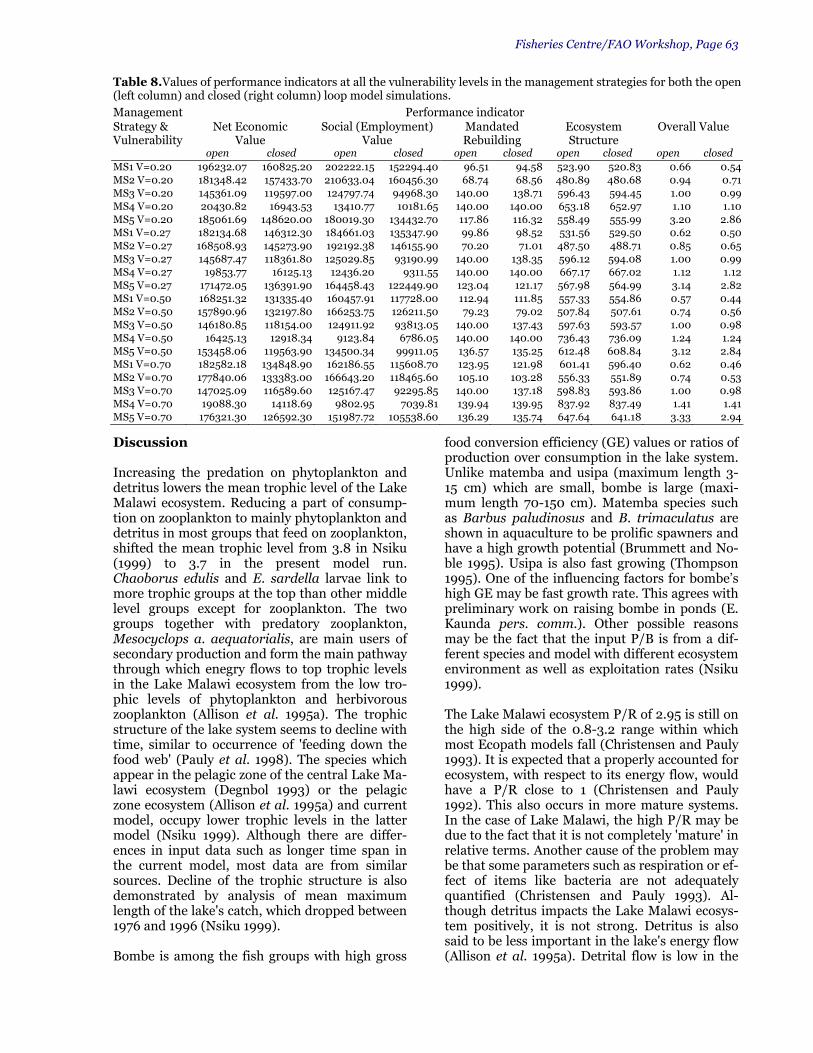
Fisheries Centre/FAO Workshop, Page 63
Discussion Increasing the predation on phytoplankton and detritus lowers the mean trophic level of the Lake Malawi ecosystem. Reducing a part of consump-tion on zooplankton to mainly phytoplankton and detritus in most groups that feed on zooplankton, shifted the mean trophic level from 3.8 in Nsiku (1999) to 3.7 in the present model run. Chaoborus edulis and E. sardella larvae link to more trophic groups at the top than other middle level groups except for zooplankton. The two groups together with predatory zooplankton, Mesocyclops a. aequatorialis, are main users of secondary production and form the main pathway through which enegry flows to top trophic levels in the Lake Malawi ecosystem from the low tro-phic levels of phytoplankton and herbivorous zooplankton (Allison et al. 1995a). The trophic structure of the lake system seems to decline with time, similar to occurrence of 'feeding down the food web' (Pauly et al. 1998). The species which appear in the pelagic zone of the central Lake Ma-lawi ecosystem (Degnbol 1993) or the pelagic zone ecosystem (Allison et al. 1995a) and current model, occupy lower trophic levels in the latter model (Nsiku 1999). Although there are differ-ences in input data such as longer time span in the current model, most data are from similar sources. Decline of the trophic structure is also demonstrated by analysis of mean maximum length of the lake's catch, which dropped between 1976 and 1996 (Nsiku 1999). Bombe is among the fish groups with high gross
food conversion efficiency (GE) values or ratios of production over consumption in the lake system. Unlike matemba and usipa (maximum length 3-15 cm) which are small, bombe is large (maxi-mum length 70-150 cm). Matemba species such as Barbus paludinosus and B. trimaculatus are shown in aquaculture to be prolific spawners and have a high growth potential (Brummett and No-ble 1995). Usipa is also fast growing (Thompson 1995). One of the influencing factors for bombe’s high GE may be fast growth rate. This agrees with preliminary work on raising bombe in ponds (E. Kaunda pers. comm.). Other possible reasons may be the fact that the input P/B is from a dif-ferent species and model with different ecosystem environment as well as exploitation rates (Nsiku 1999). The Lake Malawi ecosystem P/R of 2.95 is still on the high side of the 0.8-3.2 range within which most Ecopath models fall (Christensen and Pauly 1993). It is expected that a properly accounted for ecosystem, with respect to its energy flow, would have a P/R close to 1 (Christensen and Pauly 1992). This also occurs in more mature systems. In the case of Lake Malawi, the high P/R may be due to the fact that it is not completely 'mature' in relative terms. Another cause of the problem may be that some parameters such as respiration or ef-fect of items like bacteria are not adequately quantified (Christensen and Pauly 1993). Al-though detritus impacts the Lake Malawi ecosys-tem positively, it is not strong. Detritus is also said to be less important in the lake's energy flow (Allison et al. 1995a). Detrital flow is low in the
Table 8.Values of performance indicators at all the vulnerability levels in the management strategies for both the open (left column) and closed (right column) loop model simulations. Management Performance indicator Strategy & Vulnerability
Net Economic Value
Social (Employment) Value
Mandated Rebuilding
Ecosystem Structure
Overall Value
open closed open closed open closed open closed open closed MS1 V=0.20 196232.07 160825.20 202222.15 152294.40 96.51 94.58 523.90 520.83 0.66 0.54MS2 V=0.20 181348.42 157433.70 210633.04 160456.30 68.74 68.56 480.89 480.68 0.94 0.71MS3 V=0.20 145361.09 119597.00 124797.74 94968.30 140.00 138.71 596.43 594.45 1.00 0.99MS4 V=0.20 20430.82 16943.53 13410.77 10181.65 140.00 140.00 653.18 652.97 1.10 1.10MS5 V=0.20 185061.69 148620.00 180019.30 134432.70 117.86 116.32 558.49 555.99 3.20 2.86MS1 V=0.27 182134.68 146312.30 184661.03 135347.90 99.86 98.52 531.56 529.50 0.62 0.50MS2 V=0.27 168508.93 145273.90 192192.38 146155.90 70.20 71.01 487.50 488.71 0.85 0.65MS3 V=0.27 145687.47 118361.80 125029.85 93190.99 140.00 138.35 596.12 594.08 1.00 0.99MS4 V=0.27 19853.77 16125.13 12436.20 9311.55 140.00 140.00 667.17 667.02 1.12 1.12MS5 V=0.27 171472.05 136391.90 164458.43 122449.90 123.04 121.17 567.98 564.99 3.14 2.82MS1 V=0.50 168251.32 131335.40 160457.91 117728.00 112.94 111.85 557.33 554.86 0.57 0.44MS2 V=0.50 157890.96 132197.80 166253.75 126211.50 79.23 79.02 507.84 507.61 0.74 0.56MS3 V=0.50 146180.85 118154.00 124911.92 93813.05 140.00 137.43 597.63 593.57 1.00 0.98MS4 V=0.50 16425.13 12918.34 9123.84 6786.05 140.00 140.00 736.43 736.09 1.24 1.24MS5 V=0.50 153458.06 119563.90 134500.34 99911.05 136.57 135.25 612.48 608.84 3.12 2.84MS1 V=0.70 182582.18 134848.90 162186.55 115608.70 123.95 121.98 601.41 596.40 0.62 0.46MS2 V=0.70 177840.06 133383.00 166643.20 118465.60 105.10 103.28 556.33 551.89 0.74 0.53MS3 V=0.70 147025.09 116589.60 125167.47 92295.85 140.00 137.18 598.83 593.86 1.00 0.98MS4 V=0.70 19088.30 14118.69 9802.95 7039.81 139.94 139.95 837.92 837.49 1.41 1.41MS5 V=0.70 176321.30 126592.30 151987.72 105538.60 136.29 135.74 647.64 641.18 3.33 2.94

Page 64, Using Ecosim for Fisheries Management
trophic efficiency transfers in the lake system. This provides a clear means to designate the ma-turity of Lake Malawi ecosystem. Since detrital flow becomes more important in mature systems (Christensen and Pauly 1992; Dalsgaard 1999) it can therefore be safely said that Lake Malawi is still between the early and middle stages of its maturity. However when the formation of the East African Rift Valley is considered as well as the history of Lake Malawi, particularly of its fisheries (Potts 1999; Bertram et al. 1942), it may be more appropriate to designate the maturity of the lake to be in its middle stages. Although Ecosim has some limitations, it is very effective in simulating changes in biomasses given changes in fishing pressure (Walters et al. 1997; Christensen et al. 2000; Christensen and Walters 2000). The software has properties that are handy in the simulation of the Lake Malawi ecosystem for a period of 20 years. With the specification of the fishing mortalities, which is achieved through fixing vulnerabilities and fish-ing rates in the model, the Ecosim routine is able to effectively follow changes in fish production and potentials of all biomass pathways for the lake ecosystem during the simulation period. The choice of the model control regime, which is set at 0.25 (mixed control) for the equilibrium biomass fisheries analysis, is plausible. In the present model simulation, smooth trends of biomass over original (Ecopath equilibrium) biomass are only obtained in the vulnerability range of 0.1 and 0.29. The mixed control regime for the Lake Ma-lawi ecosystem is further based on the presence of food supply limitation, i.e. bottom-up control, which is interpreted, at least for this analysis, to have more effect than predation, i.e., top-down control. The chambo studies in the southern part of Lake Malawi (FAO 1993), experience of trophic control in the pelagic zone system in the lake (Al-lison et al. 1995b) and feeding ecology of some of the species (Yamaoka 1991) show this view clearly. The FAO chambo study, after analyzing the 1982 -1986 catches, points out the possibility of factors other than fishing (or predation) to have influenced the fish biomass and production. Allison et al. (1995b) found higher planktonic biomasses of organisms, comprising of both pro-ducers and consumers, in 1993 than 1992 which leads to increased carbon transfer in the food chain. This constitutes the evidence of their standing biomasses and production rates being controlled by food supply. It is also found that predator control is available through a rapid re-sponse of predator populations to increases in prey populations. Yamaoka (1991) emphasizes the food partitioning rather than complete food re-source sharing between species which may be as-
sumed to show superabundance of food and thus food supply not to be important in system con-trol. Cichlids of Lake Malawi have a wide range of feeding habits, although many other species com-pete for the same food resources. There is, thus, resource partitioning in fish feeding behaviour in the lake, particularly among its cichlids. This is shown by stomach content analysis, as well as de-tailed examination of species that share the same trophic requirements. They exhibit slight but clear variations in feeding ecology with regard to behaviour, sites and habitat. It is important to focus on the traditional fisheries when exploring fishing policies for Lake Malawi. This is because the sector has the majority of fish-ing operations on the lake and access to it is free (ICLARM/GTZ 1991; FAO 1993; Donda 1998). It is also difficult to manage (Scholz et al. 1997). Factors that further impact management of the sector include limitations in alternative income generating opportunities and access to adequate land, politics or sectoral conflicts, high population and resource constraints on the part of Govern-ment (GOM 1989; FAO 1993; Nyambose 1997; Scholz et al. 1997). In addition, the main fishing area for the traditional fisheries, inshore pelagic zone, is now fully exploited and expansion of the fish resources is thus not attainable (ICLARM/GTZ 1991; FAO 1993; Menz et al. 1995; Banda and Tomasson 1997). Opportunity to ex-tend to offshore is restricted by unsuitability of craft to safely navigate the offshore waters, and gears to catch demersal species (GOM 1989; Thompson et al. 1995; Banda and Tomasson 1997). One modification is made for analysis of fisheries sector landings in Lake Malawi due to unavail-ability of all commercial catches by species for the model period. However, fisheries have major im-pact on the lake ecosystem, in addition to other factors such as environmental degradation. Tradi-tional fisheries influence biomass and catch of the functional groups more than commercial fisheries at the equilibrium biomass analysis of fisheries sectors in the lake. The biomass of fish groups, which do not form fisheries in the lake particu-larly for ndunduma, mbuna, top predators and nkhono, have opposing trends to those of species-based fisheries in response to varying the fishing rates. The differences can be attributed to the fact that diets of the fish groups in the two categories overlap (Table 1). The consequence is that food supply increases when fishing rate is high as ex-ploited fish groups are depleted. Pressure for food increases when fishing rate is reduced affecting the biomasses of some groups including ndun-duma, mbuna, top predators and nkhono. This

Fisheries Centre/FAO Workshop, Page 65
observation seems to also support the concepts of food partitioning and food supply as a control re-gime for the lake's ecosystem (Yamaoka 1991; Al-lison et al. 1995b). The variation of fishing rates to above and below the equilibrium biomass level has the effect of reversing outcomes. This is probably due, in part, to vulnerability exchange in the Ecosim routine (Walters et al. 1997) as well as the fact that all other parameters for determining the biomass in the Ecopath model do not vary during simulation. The fishing policy searches optimize the lake eco-system and its fisheries mainly through decreas-ing effort. Again, the pervasive effect of the tradi-tional fisheries sector is reflected in the manage-ment goal of optimizing all objectives (MS5). The goal optimizes effort above base in the category of the sector's fisheries for the equilibrium biomass vulnerabilities 0.2 and 0.27. Like effort, the catch drops while optimizing the fisheries of the Lake Malawi system. The trend of value in the man-agement goals follows that of the catch. However, summary values for the fisheries in the lake as a whole are quite substantial at the 1996 prices. Reduction of effort and catch to optimize the management goals improves the health status of the lake ecosystem and its fisheries. The main recommendations for the development of fisher-ies in Lake Malawi from the FAO (1993) study support this view. The study finds chambo stocks fully exploited while the deep-water hap-lochromine trawl fishery is severely depleted, at least in the southeast arm of the lake. Further, the benefit of reducing effort and catch is in terms of reversing not only degradation of fish resources but also the worsening of environmental condi-tions. First, there will be regeneration of fish breeding or nesting areas as a result of reduced numbers of gears that are dragged on the lake bottom (Banda and Hara 1994). Second, overfish-ing will be abated. As a consequence species such as nchila Labeo mesops whose catches have been in decline for a long time (Tweddle et al. 1994) or overfished in the case of chambo (Oreochromis spp.) in Lake Malombe (FAO 1993) may have a chance to rebuild. The danger of certain species, which are not well known disappearing without being noticed (Munthali 1997), can be removed. Finally changes in composition of catch and fish size, which have been noticed in the southern part of Lake Malawi (Turner 1977; Tweddle and Ma-gasa 1989; Turner et al. 1995) and are probably continuing to occur, will be stopped. Conclusion The best management goal or fishing policy that optimizes exploitation and conservation of the
fish resources in Lake Malawi is to reduce the current fishing effort. In this way the ecosystem integrity of the lake or its health status, as it is now, will be maintained. Effort and thus catch may only be increased for selected offshore and demersal groups of species such as ndunduma and nkholokolo. It may have been most ideal to develop a ‘guarded’ fishery for nkhono but locally it is viewed as not edible. The potential lies in ex-ploring a market for the product first. Mbuna has the largest biomass among the fish groups in the lake. It is however not advisable to develop a fish-ery as the group is also the most diverse in num-ber of species (Ribbink 1991). An established fish-ery can easily disturb the balance and result in dissemination of some individual species in the mbuna complex. Some of the fish groups may benefit from a period of closure apart from a re-duction in fishing effort. The chambo fishery is especially in need of urgent attention. The fisher-ies of kambuzi, sanjika, mpasa as well as nchila are dwindling. In spite of the fact that utaka and kampango are largely semi-pelagic or demersal in the offshore, which limits the fishing pressure from the majority of fishers in the lake, they are still fully exploited. The six groups also require reassessment and immediate reduction from the current level of fishing effort. References Allison, E.H., G. Patterson, K. Irvine, A.B. Thompson
and A. Menz 1995a. The pelagic ecosystem, p. 351-386. In A. Menz (ed.) The fishery potential and pro-ductivity of the pelagic zone of Lake Malawi/Niassa, NRI/ODA. 386 pp.
Allison, E.H., A.B. Thompson, B.P. Ngatunga, and K. Irvine. 1995b. The diet and food consumption rates of the offshore fish, p. 233-278. In A. Menz (ed.) The fishery potential and productivity of the pelagic zone of Lake Malawi/Niassa, NRI/ODA. 386 pp.
Arnell, N., B. Bates, H. Lang, J. J. Mugnuson and P. Mulholland (Editors). 1996. Hydrology and fresh-water ecology, p. 325-363. In R. T. Watson, M.C. Zinyowera and R. H. Moss (eds.) Climate change 1995; impacts, adaptations and mitigation of cli-mate change: Scientic-technical analysis. Cam-bridge University Press. New York. 878 pp.
Banda, M. and M.Hara 1994. Habitat degradation caused by seines on the fishery of Lake Malombe and Upper Shire River and its effects. Paper pre-sented at the FAO/CIFA Seminar on Inland Fisher-ies, Aquaculture and the Environment. Harare, Zimbabwe, 5-7 December, 1994. 12 pp.
Banda, M. C. and T. Tomasson 1997. Demersal fish stocks in southern Lake Malawi: Stock assessment and exploitation, Government of Malawi, Fisheries Department, Fisheries Bulletin No. 35. 39 pp.
Banda, M., T. Tomasson and D. Tweddle 1996. Assess-ment of the deep water trawl fisheries of the south-east arm of Lake Malawi using exploratory surveys and commercial catch data, p. 53-75. In I.G. Cowx

Page 66, Using Ecosim for Fisheries Management
(ed.) Stock assessment in inland fisheries. Fishing News Books/Hartnolls Ltd. Cornwall. 513 pp.
Barel, C.D.N., R. Dorit, P.H. Greenwood, G. Fryer, N. Hughes, P.B.N. Jackson, H. Kawanabe, R. H. McConnell, M. Nagishi, A.J. Ribbink, E. Trewavas, F. Witte and K. Yamaoka 1985. Commentary: De-struction of fisheries in Africa's lakes. Nature 315: 19-20.
Beadle, L.C. 1974. The inland waters of tropical Africa: An introduction to tropical limnology, Longman, London. 365 pp.
Berlin, B. 1992. Ethnobiological classification: Princi-ples of categorization of plants and animals in tradi-tional societies. Princeton University Press, Prince-ton. 335 pp.
Bertram, C. K. R., H. J. H. Borley and E. Trewavas 1942. Report on the fish and fisheries of Lake Nyasa. Published on behalf of the Government of Nyasaland [Malawi] by the Crown Agents of the Colonies, London. 181 pp.
Brummett, R.E. and R. Noble 1995. Aquaculture for Af-rican smallholders. Manila, Philippines. ICLARM Tech. Rep. 46. 69 pp.
Bundy, A. 1997. Assessment and management of mul-tispecies, multigear fisheries: a case study from San Miguel Bay, Philippines. Ph.D. Thesis University of British Columbia, Vancouver, B.C., Canada. 396 pp.
Christensen, V. and D. Pauly 1992. A guide to Ecopath II software system (version 2.1). ICLARM. Software. 6. 72 pp.
Christensen, V. and D. Pauly. 1993. Flow characteristics of aquatic ecosystems. Pages 338-352 in V. Chris-tensen and D. Pauly (eds.) Trophic models of aquatic ecosystems. ICLARM Conf. Proc. 26. 390 pp.
Christensen, V, C.J. Walters and D. Pauly. 2000. Eco-path with Ecosim: a User's Guide, October 2000 Edition. Fisheries Centre, University of British Co-lumbia, Vancouver, Canada and ICLARM, Penang, Malaysia. 130 pp (accessible on website http://www.ecopath.org).
Christensen, V. and C.J. Walters 2000. Ecopath with Ecosim: methods, capabilities and limitations. 26 pp. (accessible on website http:// www.fisheries.ubc.ca).
Dalsgaard, A.J. 1999. Modelling the trophic transfer of beta radioactivity in the marine food of the Enewetak Atoll, Micronesia. MSc. thesis. University of British Columbia, Vancouver, B.C., Canada. 125 pp.
Degnbol, P. 1993. The Pelagic Zone of Central Lake Ma-lawi: A Trophic box model. Pages 110-115 in V. Christensen and D. Pauly (eds.) Trophic models of aquatic ecosystems. ICLARM Conf. Proc. 26. 390 pp.
Donda, S. 1998. Fisheries co-management in Malawi: Case study of Lake Chiuta fisheries, p.21-39. In A.K. Norman, J.R. Neilsen and S. Sverdrup-Jensen (eds.) Fisheries co-management in Africa. Fish. Co-mgmt. Res. Project, Res. Rpt. 12. 326 pp.
Eccles, D. H. 1962. An internal wave in Lake Nyasa (now Malawi) and its probable significance in the nutrient cycle. Nature 194(4831): 832-833.
FAO 1993. Fisheries management in the southeast arm of Lake Malawi, the Upper Shire River and Lake Malombe, with particular reference to the fisheries
on chambo (Oreochromis spp.). CIFA Technical Paper. No. 21. Rome, FAO. 113 pp.
Government of Malawi (GOM) 1989. Statement of de-velopment policies, 1987-1996. Government Printer, Zomba, Malawi. p. 1-21, 42-48.
Government of Malawi and United Nations in Malawi (GOM/UN) 1992. The situation analysis of poverty in Malawi (Draft). UNICEF. Lilongwe. 202 pp.
Government of Malawi 1997. Economic report 1997. Ministry of Economic Planning and Development, Government Printer, Zomba, Malawi. 118 pp.
ICLARM/GTZ 1991. The context of small-scale inte-grated agriculture-aquaculture in Africa: a case study of Malawi. ICLARM Stud. Rev. 18. 302 pp.
IMF 1998. IMF approves third annual ESAF credit for Malawi, Press release No. 98/63. IMF, Washington, D.C. 14 pp (accessible on website http:// www.imf.org).
Malawi Fisheries Department (MFD) 1996. Fisheries statistics (unpublished). 12 pp.
Menz, A. (ed) 1995. The fishery potential and produc-tivity of the pelagic zone of Lake Malawi/Niassa, NRI/ODA, 386 pp.
Munthali, S.M. 1997. Dwindling food-fish species and fishers’ preference: problems of conserving Lake Malawi’s biodiversity. Biodiversity and Conserva-tion 6: 253-261.
Nsiku, E. 1999. Changes in the fisheries of Lake Ma-lawi, 1976-1996: Ecosystem-based analysis. M.Sc. thesis. University of British Columbia, Vancouver, Canada. 217 pp.
Nyambose, J. 1996. Preserving the future of Lake Ma-lawi. Afrian Technology Forum. MIT 6 p. (accessi-ble on website http://web.mit.edu/ african-tech/www/articlesLake-Malawi.html).
Patterson, G. and O. Kachinjika 1995. Limnology and phytoplankton ecology. Pages 1-67 in A. Menz (ed.) The fishery potential and productivity of the pelagic zone of Lake Malawi/Niassa. NRI/ODA. 386 pp.
Patterson, G., M.J. Wooster and C.B. Sear 1995. Real-time monitoring of African aquatic resources using remote sensing: with special reference to Lake Ma-lawi. Chatham, UK: Natural Resources Institute. 21 pp.
Pauly, D., V. Christensen, J. Dalsgaard, R. Froese and F. Torres 1998. Fishing down marine foodwebs. Science 279: 860-863.
Pitcher, T.J. 1994. Results: impact of species changes on fisheries in Lake Malawi. Pages 81-84 tn T.J. Pitcher (ed) The impact of species changes in the African lakes. Report to the Overseas Development Administration, London, UK. 213 pp.
Potts, R. 1999. Executive summary of the workshop re-port on an NSF/ICDP workshop on scientific drill-ing on Lakes Malawi and Tanganyika [The Lake Malawi drilling project] October 10-16, 1999 Club Makakola, on the southwestern lakeshore of Lake Malawi. National Museum of Natural History, Smithsonian Institution, Washington (accessible on website http://malawidrilling.syr.edu/report2. html).
Ribbink, A. J. 1991. Distribution and ecology of the cichlids of the African Great Lakes. Pages 36-59. in M.H.A. Keenleyside (ed.) Cichlid fishes: Behaviour, ecology and evolution. Chapman & Hall. Fish and Fisheries Series 2.

Fisheries Centre/FAO Workshop, Page 67
Scholz, U.F., F.J. Njaya, S. Chimatiro, M. Hummel, S. Donda and B.J. Mkoko 1997. Status and prospects of participatory fisheries management programmes in Malawi: A paper presented at the FAO/ODA ex-pert consultation on inland fisheries enhancements, Dhaka, Bangladesh, 7-11 April, 1997. 12 pp.
Snoeks, J. (ed.) 2000. Report on systematics and tax-onomy: SADC/GEF Lake Malawi/Nyasa/Niassa Biodiversity Conservation Project. Tervuren, Bel-gium [Chapter 1, p. 1-14 of modified report from the editor].
Thompson, A.B. 1995. Eggs and larvae of Engrauli-cypris sardella, p. 179-199. In A. Menz (ed.) The fishery potential and productivity of the pelagic zone of Lake Malawi/Niassa, NRI/ODA. 386 pp.
Thompson, A.B., E.H. Allison and B.P. Ngatunga. 1995. Spatial and temporal distribution of fish in the pe-lagic waters, p. 201-232. In A. Menz (ed.) The fish-ery potential and productivity of the pelagic zone of Lake Malawi/Niassa, NRI/ODA. 386 pp.
Turner, J. L. 1977. Some effects of demersal trawling in Lake Malawi (Lake Nyasa) from 1968 to 1974. J. Fish. Biol. 10: 261-271.
Turner, G. F. 1995. Management, conservation and species changes of exploited fish stocks in Lake Ma-lawi, Pages 335-395 in T.J. Pitcher and P.J.B. Hart (eds.) The impact of species changes in African Lakes. Chapman and Hall. Fish and Fisheries Series 18.
Turner, G. F., D. Tweddle and R. Makwinja. 1995. Changes in demersal cichlid communities as a re-sult of trawling in southern Lake Malawi, p. 397-412. In T.J. Pitcher and P.J.B. Hart (eds.) The im-pact of species changes in African Lakes. Chapman and Hall. Fish and Fisheries Series 18.
Turner, G. F. 1996. Offshore cichlids of Lake Malawi. Cichlid Press. Lauenau. 240 pp.
Tweddle, D. and J. H. Magasa 1989. Assessment of multispecies cichlid fisheries of the southeast arm of Lake Malawi, Africa. J. Cons. int. Explor. Mer 45: 209-222.
Tweddle, D, S.B. Alimoso and G. Sodzapanja 1994. Analysis of catch and effort data for the fisheries of the South East Arm of Lake Malawi, 1976-1989 with a discussion on earlier data and inter-relationships with commercial fisheries. Malawi Fisheries De-partment, Fisheries Bulletin No. 13. 34 pp.
Walters, C., V. Christensen and D. Pauly 1997. Struc-turing dynamic models of exploited ecosystems from trophic mass-balance. Reviews in Fish Biology and Fisheries 7: 1139-1172.
WWF 1999. Lake Malawi national park, Malawi. Inter-national Reports. 1 pp (accessible on website http://www.panda.org).
Yamaoka, K. 1991. Feeding relationships, p. 151-172. In M.H.A. Keenleyside (ed.) Cichlid fishes: Behaviour, ecology and evolution. Chapman & Hall. Fish and Fisheries Series 2.

Page 68, Using Ecosim for Fisheries Management
The use of Ecosim to investigate multispecies harvesting strategies for capture fisheries of the Newfoundland-Labrador shelf Marcelo Vasconcellos1, Johanna Heymans1
and Alida Bundy2 1Fisheries Centre, UBC 2 Bedford Institute of Ocenaography, Darmouth, Nova Scotia Abstract
This paper evaluates the policy optimization routine of Ecopath/Ecosim using as case study the model of the Newfoundland-Labrador shelf for the period 1985-1987. The routine is used to calculate the best combina-tion of harvesting strategies for multiple fleets and to il-lustrate the type of tradeoffs expected when fisheries management aims at maximizing economic, social and ecological goals. To maximize social and economic re-turns from the fishery the optimization routine drives the ecosystem to a very simplified state where high tro-phic level species are depleted and low trophic level species have a net increase in biomass after 20 years of simulation. To maximize ecological stability the model predicts in almost all cases a substantial decrease in all fishing fleets. The performance of calculated optimal harvesting strategies are generally affected by increas-ing errors in stock assessment procedures. More realis-tic analysis of future fisheries management policies for the Newfoundland-Labrador shelf will require more accurate data for prices per species, fleet operational costs, employment indicators for each fishery, and also ecological parameters that better represent the current status of the ecosystem
Introduction The objective of this paper is to evaluate the use of Ecosim, a quantitative ecosystem model struc-tured from Ecopath mass-balance assessment, in
the analysis of the ecological and socio-economic impacts of hypothetical fisheries strategies for the Newfoundland-Labrador shelf marine ecosystem. A mass balance model of the Newfoundland-Labrador shelf for the period 1985-1987 ( Fig. 1; Bundy et al., 2000) was used in the simulation of the impact of fisheries strategies. The model represents the main functional groups, trophic flows and fisheries in the Northwest Atlantic Fisheries Organization (NAFO) areas 2J3KL and 3NO, corresponding to the regions of the Labra-dor shelf, the Northeast Newfoundland shelf and the Grand Bank, from the coast to the 1,000 m isobath. A total of 31 functional groups are repre-sented in the model, including phyto- and zoo-plankton, benthic organisms, invertebrate stocks, pelagic and demersal fish stocks, seabirds, seals and whales. Also, three species of fish, Northern cod, Greenland halibut and American plaice were divided into adult and juvenile pools to account for ontogenic differences in diets. The largest and most important fish stock in the region was the Northern cod. The model represents a period of relatively constant abundance of the main com-mercially harvested groundfish stocks, prior to the collapse of the Northern cod stock. Five main fleet types are represented in the model (Table 1): inshore trawlers, offshore trawlers directed to cod, American plaice and other groundfish spe-cies, mixed gear (including seine nets, gillnets and lines), foreign trawlers, and fleets targeting seals and seabirds. The analysis aimed at using the policy optimiza-tion routine in Ecosim to define i) the best com-bination of harvesting strategies (relative fishing effort) according to different goal functions, and ii) to calculate the expected or achievable per-formance when errors in stock assessment proce-dures over time are accounted for (closed loop scenario).
Table 1: Catches and trophic level of the species caught by 5 fleet types of the Newfoundland-Labrador shelf region represented in the model. TL = Trophic level.
Harvested groups
TL
Inshore trawlers
Offshore trawlers
Mixed gears
Foreign trawlers
Sealing and seabirds
Total
Greenland halibut>40cm 4.5 0.004 0.017 0.016 0.037Harp Seals 4.4 0.001 0.001 Greenland halibut<=40cm 4.3 0.001 0.001 Seabirds 4.2 0.001 0.001 Cod > 35cm 4.2 0.014 0.257 0.164 0.150 0.585Large pelagic feeders 4.2 0.002 0.003 0.005 Piscivore small pelagic fish 4.1 0.015 0.001 0.016 Skates 4.0 0.030 0.030 American plaice<=35cm 3.7 0.004 0.016 0.020Redfish 3.7 0.001 0.042 0.001 0.132 0.176 American plaice>35cm 3.6 0.003 0.059 0.009 0.029 0.100 Large demersal feeders 3.4 0.002 0.012 0.007 0.036 0.057Capelin 3.3 0.082 0.044 0.126Planktivore small pelagic fish 3.3 0.019 0.001 0.020Flounders 3.1 0.002 0.033 0.004 0.039 0.078Large Crustacea 2.9 0.016 0.016 Shrimp 2.5 0.001 0.002 0.003 Total by fleet 0.022 0.413 0.336 0.499 0.002 1.272

Fisheries Centre/FAO Workshop, Page 69
Methods Three performance indicators are used by the op-timization search procedure (Christensen et al., 2000): Net economic value: measured as the total landed value of catch minus total operating cost over a 20 year period, with a discount rate of 4%. Operating costs were assigned to fixed costs (35% of total value) and ef-fort-related costs (20% of total value) for all fleets. Employment: measured as the product of the gross landed value of the catch and the jobs per landed value ratio for each fleet, i.e. inshore trawlers (5); offshore trawlers (1); mixed gears (5); foreign trawlers (0.1); seals and seabirds fleet (5). Ecological stability: measured by the departure (nega-tive) of species biomasses over time from target bio-mass levels specified for each functional group. Eco-logical stability attempts to capture the importance of each species/group to the overall ‘health’ of the ecosys-tem, as defined by managers. During simulations we assumed that whales, seals, seabirds and cod are im-portant for managers and that it is their goal to rebuild the biomass of these groups to 3 times the baseline Ecopath value. Additionally, we tested species weight-ings proportional to the inverse of the P/B ratio, which provided simil qualitative results. By assigning weights to each of the three indica-tors it was then possible to define different man-agement goals and strategies (Table 2) (and see
Cochrane this volume). Besides the three man-agement goals in Table 2, we examined how poli-cies would change in response to increasing weights to ecological stability, starting from an equal weight scenario (1 to economic, 1 to em-ployment, and 1 to ecological stability). Simulations were run under two trophic control scenarios, expressed by the value of the prey vul-nerability parameter: v=0.4 and v= 0.6. During simulations adult and juvenile Greenland halibut presented alternated cycles in abundance that forced us to adjust feeding time to increase model stability (ca. 13% of the diet of adult hali-but is made of juvenile halibut). Feeding time fac-tor of adult and juvenile Greenland halibut was thus set to 0, thus feeding time and hence the time exposed to predation is forced to remain constant, and less dependent on changes in prey availability.
Table 2. Management goals and performance indica-tors used in the optimization procedure.
Weights for performance indicators
Management goal
Net eco-nomic value
Employment Ecological stability
Maximize net economic value 1.000 0.0001 0.0001 Maximize em-ployment 0.0001 1.000 0.0001 Maximize eco-logical stability 0.0001 0.0001 1.000
Figure 1. Trophic model of the Newfoundland-Labrador shelf area during the 1985-1987 period (Bundy et al., 2000).

Page 70, Using Ecosim for Fisheries Management
Simulation results Table 3 shows the results of the policy optimiza-tion for three contrasting management goals. In order to meet the economic goal of maximizing the net economic return taken from the system the model calculates a reduction in inshore and offshore trawlers and an increase in mixed gears, foreign trawlers and the harvesting of seals and sea birds. In this scenario the best solution seems to be to increase the relative fishing effort of the fleets with highest yields (mixed gears and foreign trawlers), which also target low trophic level spe-cies (Table 1), and to deplete the top predators in the system (seals and birds), which are competi-tors to fisheries. To meet the social goal of maximizing employ-ment the optimal policy involves an increase in all fishing fleets, particularly mixed gears that have a higher jobs/landings ratio. To maximize ecologi-cal stability the model predicts in almost all cases a substantial decrease in all fishing fleets. Predic-tions of optimal fishing rates and performance values are sensitive to the value of the vulnerabil-ity parameter, although the general qualitative pattern of predictions is similar under both tro-phic control scenarios. Figure 2 shows the result-ing changes in species biomass under optimal policies for each management goal. In order to maximize economic return and employment (measured as a variable dependent on landings) the hypothetical manager drives the system to a very simplified state where high trophic level spe-cies are depleted and low trophic level species have a net increase in biomass. There are two ap-parent factors contributing to increasing land-ings; firstly the increase in fishing pressure on the groundfish stocks (some of them completely col-lapsed after 20 years); and secondly, the increase in biomass and hence the productivity of lower trophic level species also targeted by fisheries (e.g. shrimps, capelin, planktivorous fish). A more balanced distribution of biomass across the food
web is obtained when the goal is to maximize ecological stabil-ity. Releasing fishing pressure leads to a system that presents at the end of the simulation similar characteristics encoun-tered at the starting condition. Figure 3 compares policy per-formance with increasing weight given to ecological sta-bility. Relatively small changes in policy performance occur up to a 1:1:10 weighting to eco-
nomic, social and ecological goals, respectively, which is achieved with the following relative fish-ing rates (Table 4):
Increasing the weight for ecological stability even more leads to more drastic changes in the three performance indicators, as well as in the calcu-lated optimal fishing rates (Table 5).
This example is illustrative of the type of tradeoffs encountered when managers aim at balancing ecological and socio-economic goals. Using the simple goal functions specified above, the model predicts that improvements in ecological per-formance will occur at the expense of substantial losses in socio-economic performance (Figure 3). Interestingly, the optimal policy calculated by the model in the latter scenario is the one that closes fisheries with low jobs/catch ratio (offshore and foreign trawlers) and also the direct harvesting of charismatic fauna. The effect of the lack of perfect information about stock sizes and the actual fishing mortality on the performance of policies were also considered in the simulations. Ecosim evaluates the perform-ance of fishing strategies in a closed loop scheme where managers have to rely on stock assessment to determine the annual optimal policies. Typically, errors in stock assessment cause vari-
Table 3. Performance indicators of optimal policies (relative Fs) under two trophic control (= vulnerability) scenarios (v=0.4 and 0.6).
V=0.4 V=0.6 Goal
Eco-nomic
Social
Ecologi-cal
Eco-nomic
Social
Ecologi-cal
Performance Net economic value 155.4 87.4 8.8 292.2 240.6 42.1 Employment 1027.1 1101.8 17.5 1562.6 1782.2 24.6 Ecological stability -709.0 -727.1 -420.3 -1027.3 -632.5 -407.2 Overall 3.3 10.7 -1.2 6.2 17.2 -1.1
Optimal Fs by fleet Inshore trawlers 0.4 2.8 0.5 1.1 7.3 0.6 Offshore trawlers 0.1 20.1 0.1 0.0 21.1 0.2
Mixed gears 20.1 76.8 0.1 274.0 20.4 0.2 Foreign trawlers 6.9 10.2 0.1 24.9 3.8 4.6
Sealing, birds 6.6 13.1 0.1 0.1 3.9 0.1
Table 4. Relative fishing rates. Inshore trawlers 2.3 Offshore trawlers 0.0 Mixed gears 2.0 Foreign trawlers 0.0 Seals and seabirds 0.0
Table 5. Optimal fishing rates. Inshore trawlers 8.6 Offshore trawlers 0.3 Mixed gears 20.5 Foreign trawlers 10.8 Seals and seabirds 0.8

Fisheries Centre/FAO Workshop, Page 71
ability in the implemented fishing rates and hence affect the performance of fishing strategies. In the example below the performance of a policy that optimizes the balance among economic, social and ecological goals is evaluated under three lev-els of observation errors (Table 6: coefficient of variation of the stock assessment procedure). We found that there is a general decrease of per-formance for economic, social and overall indica-tors, but a slight improvement in ecological per-formance with increasing error, meaning that the
variability imposed by stock assessment error is predicted to actually attenuate the impact of fish-ing on ecological stability. In all cases we tested, ecological stability either improved or remained relatively unchanged with increasing assessment
Table 6. Coefficient of variation of the stock as-sessment procedure CV=0 CV=0.2 CV=0.5 Economic 150.3 121.6 111.9 Social 1058.5 780.7 702 Ecological -677.9 -662.6 -657.3 Overall 11.5 8.28 7.33
economic goal
00.5
11.5
22.5
3
Hoode
d Sea
ls
G.halib
ut>40
cm
Harp Sea
ls
G.halib
ut<=4
0cm
Whales
Seabir
ds
Cod >
35cm
L.Pel.
Feede
rs
Pisc. S
PFSka
tes
Cod <=
35 cm
Aplaice
<=35
cmRed
fish
Aplaice
>35c
m
Arctic
cod
L.Dem
.Feede
rs
Capeli
n
Plankt.
SPF
Sand l
ance
Flound
ers
S.Dem
.Feede
rs
Large
Crus
tacea
Shrimp
Ben
d/B
star
t
social goal
0
0.5
1
1.5
2
2.5
3
Hoode
d Sea
ls
G.halib
ut>40
cm
Harp Sea
ls
G.halib
ut<=4
0cm
Whales
Seabir
ds
Cod >
35cm
L.Pel.
Feede
rs
Pisc. S
PF
Skates
Cod <= 3
5 cm
Aplaice
<=35
cm
Redfis
h
Aplaice
>35c
m
Arctic
cod
L.Dem
.Feede
rs
Capeli
n
Plankt.
SPF
Sand l
ance
Flound
ers
S.Dem
.Feede
rs
Large
Crus
tacea
Shrimp
Ben
d/B
star
t
ecological goal
0
0.5
1
1.5
2
2.5
3
Hoode
d Sea
ls
G.halib
ut>40
cm
Harp Sea
ls
G.halib
ut<=4
0cm
Whales
Seabir
ds
Cod > 35
cm
L.Pel.
Feede
rs
Pisc. S
PF
Skates
Cod <=
35 cm
Aplaice
<=35
cm
Redfis
h
Aplaice
>35c
m
Arctic
cod
L.Dem
.Feede
rs
Capeli
n
Plankt.
SPF
Sand l
ance
Flound
ers
S.Dem
.Feede
rs
Large
Crus
tacea
Shrimp
Ben
d/B
star
t
Figure 2. Predicted changes in biomass of functional groups of Newfoundland-Labrador shelf model as a result of fishing rates that optimize economic, social and ecological goal functions. Bend/Bstart is the ratio between biomass at the start of the simulation and at the end of 20 years period under the same fishing rate. Results are presented for 23 groups placed in order of decreasing trophic level from left to right.

Page 72, Using Ecosim for Fisheries Management
errors. Conclusion The analysis presented above was not meant to provide a realistic policy evaluation for the model area. Instead the goal was to test the overall be-havior of the model un-der different parameter settings, and to check the consistency of the results according to the different policy scenarios. A more realistic analysis should include better economic data (prices per species, fleet operational costs), better social indicators (such as employment for each fishery) and also ecological parameters that better represent the current status of the system and its ecosystem dynamics. Of particular importance are the vul-nerability parameters among species, which seems to influence the magnitude of performance values and optimal fishing rates. When running the policy optimization routine attention should also be given to long term changes in productiv-ity, or oceanic regimes, which might influence the overall performance of policy options considera-bly. References Bundy, A., Lilly, G. R. and P. A. Shelton 2000. A mass
balance model of the Newfoundland-Labrador shelf. Canadian Technical Report of Fisheries and Aquatic Sciences.
Christensen, V., C.J. Walters, and D. Pauly 2000. Eco-path with Ecosim Version 4: Help System. Univer-sityof British Columbia, Fisheries Centre, Vancou-ver, Canada and ICLARM, Penang, Malaysia
-800
-600
-400-200
0
200
400
600800
1000
1200
1 5 10 20 30
Ecological weight
Perf
orm
ance econ
socioecol
Figure 3. Changes in policy performance with increasing weight given to ecological stability. The x axis represents the weight given to ecological stability when eco-nomic and social weights are kept constant at 1.

Fisheries Centre/FAO Workshop, Page 73
Simulating management options for the North Sea in the 1880s Steven Mackinson CEFAS, Lowestoft, UK Abstract An Ecopath model of the North Sea in the 1880s, is used here in evaluating the utility of the Ecosim policy simulation routine. The model representation of the North Sea in the 1880s was 're-constructed' by combin-ing present information on trophic linkages of North Sea species with historical scientific and local knowl-edge. The model captures the period when sailing ves-sels still predominated and industrialised fishing was on the cusp of explosive development. Evaluation of Ecosim policy simulation routines focussed on sensitiv-ity analysis in relation to: (i) initialisation options of optimisation routines, (ii) the effect of the user input vulnerability flow rate parameter, v, (iii) parameter set-tings for the 'closed-loop' analysis of management er-rors. By providing users with tools to examine various policy options and objectively comparing them using criteria scores, the policy evaluation options contribute great utility to the Ecopath with Ecosim software. However, it is important to re-iterate that users should not interpret criteria scores as providing direction for management advice; results of simulations depend heavily on specific parameter settings used. In particu-lar, simulations are very sensitive to the user input vul-nerability flow rate. Specific noteworthy points/ issues arising from the simulations are commented on. Introduction: Ecopath Model of The North Sea in the 1880’s Prior to the development of steam fishing vessels in the early 1880s, more than 30,000 sailing fishing ves-sels, from bordering coun-tries, ploughed the boun-tiful waters of the North Sea. In the UK alone, fishing and its associated activities provided a liveli-hood for upwards of 100,000 people. The North Sea was particularly rich in marine life, both in general and in individual populations. Outstripping all in economic and socio-logical significance, how-
ever, was one fish; the herring (Fig. 1). Herring drifters and beam trawling sailing smacks (Fig. 2) dominated the seas with other small vessels en-gaging in hook and line fishing and crab and lob-sters in coastal waters. Trawl fish were classified under the names ‘prime’ and ‘offal’; the former including turbot, brill, soles, and Doreys; the lat-ter comprising plaice, cod, haddocks, gurnards, skate, and “other such kinds as are occasionally caught in the trawl” (Holdsworth 1874) (Fig 3). Combining present information on trophic link-ages of North Sea species with historical scientific and local knowledge, an ecosystem model is re-constructed to describe the state of the North Sea ecosystem in the 1880s (Mackinson 2000). The model is ‘re-constructed’ with the aid of a previ-ous model describing the state of the ecosystem in 1980s (Christensen 1995). Simulation settings The 1880’s North Sea model consists of 44 groups and 5 fisheries. Trawl and line fisheries are com-bined in to one group since they catch the same species and no information was readily available to otherwise separate them. Settings used during simulations of various management policy op-tions examined below are detailed in Appendix 1 (Tables i, ii and iii) and made reference to in the text.
0
100,000
200,000
300,000
400,000
500,000
1808 1818 1828 1838 1848 1858 1868 1878 1888 1898
tonn
es
HollandScotlandEnglandGermanyBelgiumDenmarkFranceNorwayTOTAL ESTIMATED HERRING CATCH
Figure 1. Catch of North Sea herring. The apparent sharp dip in catches from the late 1870s to mid 1880s is not real, but due to missing catch statistics for the Scottish fleet during that period.

Page 74, Using Ecosim for Fisheries Management
Effect of initialisation options on estimates of relative fishing mortality derived from a search procedure used to define an optimum harvest strategy in terms of fishing mortality for each gear type Prior to examining the influence of alternative weightings on the economic, social and ecological importance of management policy options, it was essential to explore the effect of the three initiali-sation options on the results of the optimum har-vest strategy search procedure (conjugate gradi-ent method). The options for search initialisation were consid-ered individually and combined. Those compared were: 1. Start at Ecopath base values (EB) 2. Random start (R) 3. Start from Ecopath base and restart using Current
values (EB+C) 4. Random start and restart using current values
(R+C) For each of the initialisation settings, the search procedure was allowed to run three times. The stability of the relative F estimates was compared between runs and between initialisation options (Fig 4).
Searches starting from Ecopath base (EB) ob-tained the same consistent relative F values. However, these were considerably different from all other remaining searches. The random search method and combined EB+C and R+C initialisa-tions derived relative fishing mortality estimates in approximately the same ratios for the 5 gear types, although neither consistent nor stable rela-tive F values were derived within or between ini-tialisation options. Based on these results, for consistency, the strat-egy used in all subsequent simulations of al-ternative policy options was to run the search procedure starting at Ecopath base F values, al-lowing the procedure to run for at least 2 times the number of gear types, then to re-run the search starting from current F values. Unless any relative F values estimates were greater than 20 times the initial F (a constraint within the search procedure indicating that such values are non-
Figure 2. Yarmouth Lugger drift net fishing for her-ring at night (top), and trawling smack towing the trawl (Holdsworth 1874)
Figure 3. North Sea catches of cod, haddock, soles, brill, salmon, sturgeon, mackerel and turbot and plaice from 1850 to 1902.
0
500
1,000
1,500
2,000
2,500
3,000
3,500
4,000
4,500
1850 1860 1870 1880 1890 1900
tonn
es
Brill TurbotSoles MackerelSalmon Sturgeon
0
50,000
100,000
150,000
200,000
250,000
1865 1870 1875 1880 1885 1890 1895 1900 1905
tonn
es
CodPlaiceHaddock

Fisheries Centre/FAO Workshop, Page 75
sense), the relative F estimates were used in simulations. For the cases where estimated F’s exceeded 20 times initial F, the search procedure was run again with a random start and re-run us-ing current F’s. Influence of flow control parameter The flow control (= vulnerabilty) parameter specifies the flow between invulnerable and vul-nerable prey, and from prey to predator. Higher values of flow rapidly replenish the vulnerable prey pool from the invulnerable pool, indicating that food is not limiting and thus representing more ‘top down’ control. Lower values (e.g. 0.2) represent low flow of food, thus representing a ‘bottom up’ control effect on the predator-prey in-teractions. Intermediate values (e.g. 0.5) repre-sent mixed control. The flow control thus has im-portant consequences to the dynamics of the in-teractions in the model and simulations must be compared under various settings. Whilst there are several methods implemented in Ecosim to derive values of flow control between various groups, the present analysis simply compares 3 values of the parameter, each applied as a ‘blanket’ setting for
all groups in the model. The effect of flow con-trol on the estimation of F during the search procedure was com-pared for 4 policy scenarios (see next section for details of scenarios). Values of flow control above 0.6 generally produced unstable dynamics of the model. From Fig-ure 5 it appears there are no apparent trends in the effect of flow control on the estimation of opti-mum F. In the eco-nomic maximisation scenario, lower flow control results in higher estimates of F for most gears, sug-
gesting that fished groups are more resilient at low flow control. However, this observation does not hold true for ‘other’ gear, nor across alterna-tive policy scenarios. The effect of the flow control on the resilience of a group to fishing is unclear and rather confusing. It appears to fluctuate de-pending on what group is being fished, and the assumptions of the policy being considered. I have doubt as to whether or not the lack of ‘pat-tern’ in response to changes in flow control is a result of differences in the fishing mortality esti-mates derived from the search procedure. My conclusion is one of caution; once a particular policy has been chosen, the response to changes in the assumptions of flow control should be thoroughly examined. However, it still remains unclear to me how changes in the flow control ef-fect the response of each group to fishing, since fishing mortality is not directly linked with the flow control parameter. Comparison of setting all flow control to v=0.4 with prey vulnerabilities assumed to be propor-tional to trophic level
Table 2. Weighting assigned to each value component under 4 policy scenarios
Value weight for each scenario
Value Component 1. Economic
maximisation 2. Social
maximisation 3. Ecological
maximisation 4. ‘Big compro-
mise’ Net economic value 1 0.00001 0.00001 1 Social (employment) value 0.00001 1 0.00001 1 Ecosystem stability 0.00001 0.00001 1 1
0
0.5
1
1.5
2
2.5
EB1 EB2 EB3 R1 R2 R3 EB+C1 EB+C2 EB+C3 R+C1 R+C2 R+C3
Search method
Rel
ativ
e fis
hing
mor
talit
yDriftersTrawlers and liners
OthersPots
Seal killing
Figure 4. Comparison of stability of F estimates from search procedures
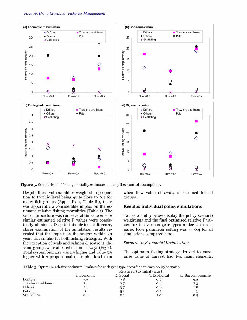
Page 76, Using Ecosim for Fisheries Management
Despite those vulnerabilities weighted in propor-tion to trophic level being quite close to 0.4 for many fish groups (Appendix 1, Table iii), there was apparently a considerable impact on the es-timated relative fishing mortalities (Table 1). The search procedure was run several times to ensure similar estimated relative F values were consis-tently obtained. Despite this obvious difference, closer examination of the simulation results re-vealed that the impact on the system within 20 years was similar for both fishing strategies. With the exception of seals and salmon & seatrout, the same groups were affected in similar ways (Fig 6). Total system biomass was 1% higher and value 5% higher with v proportional to trophic level than
when flow value of v=0.4 is assumed for all groups. Results: individual policy simulations Tables 2 and 3 below display the policy scenario weightings and the final optimised relative F val-ues for the various gear types under each sce-nario. Flow parameter setting was v= 0.4 for all simulations compared here. Scenario 1: Economic Maximisation The optimum fishing strategy derived to maxi-mise value of harvest had two main elements.
Table 3. Optimum relative optimum F values for each gear type according to each policy scenario
Relative F (to initial value) 1. Economic 2. Social 3. Ecological 4. ‘Big compromise’ Drifters 7.9 9.8 0.6 9.2 Trawlers and liners 7.1 9.7 0.4 7.3 Others 2.1 3.7 0.8 2.8 Pots 1 5.1 0.5 1.3Seal killing 0.1 0.1 1.8 0.9
(a) Economic maximimum
0
5
10
15
20
25
30
Flow =0.6 Flow =0.4 Flow =0.2
Reat
ive
Fish
ing
mor
tality
Drif ters Traw lers and linersOthers PotsSeal killing
(b) Social maximum
0
5
10
15
20
25
Flow =0.6 Flow =0.4 Flow =0.2
Reat
ive
Fish
ing
mor
tality
Drifters Traw lers and linersOthers PotsSeal killing
(c) Ecological maximimum
0
0.5
1
1.5
2
2.5
3
3.5
4
Flow =0.6 Flow =0.4 Flow =0.2
Reat
ive
Fish
ing
mor
tality
Drifters Traw lers and linersOthers PotsSeal killing
(d) Big compromise
0
5
10
15
20
25
30
Flow =0.6 Flow =0.4 Flow =0.2
Reat
ive
Fish
ing
mor
tality
Drifters Traw lers and linersOthers PotsSeal killing
Figure 5. Comparison of fishing mortality estimates under 3 flow control assumptions.

Fisheries Centre/FAO Workshop, Page 77
First was to increase the harvest pressure for both the high valued ‘prime’ fish (via trawl gear) and on the lower value, higher volume, herring (via Drifter fleet). The low initial fishing moralities were increased approximately seven fold in each case. The second element comprised a 2 times in-crease in F for ‘other’ gear (acting on bluefin tuna, saithe, salmon & seatrout, mackerel, and sprat) which resulted in the main predators herring and ‘prime fish’ being reduced, thus alleviating the predation pressure on them. Ironically, salmon & seatrout ended up benefiting from the increased fishing pressure (on themselves from the ‘other’ gear), as a result of release of euphasiid food, when the herring stock declined. Other ‘winners’ and ‘losers’, (only those whose biomass at the end of the run was > ±20% that at the start) are shown in Fig 7a. The stocks of herring and ‘prime’ fish were maintained throughout the period de-spite the early heavy fishing mortality. Total bio-mass of all groups was 11% less at the end of the run than the start. Whilst there was reduction in total value of the fishery by 32%, total value re-mained 2 times that of the costs. Scenario 2: Social (Jobs) Maximisation Attempting to maximise the jobs/catch ratio of the combined fisheries, results in a similar har-vest strategy to the economic maximisation pol-icy. This is unsurprising since according to the distribution of average crew sizes (14 for Drifters, 9 for trawlers, 6 for ‘others’, 3 for pots) the largest number of jobs per unit catch would be made
available in the herring fishery, fol-lowed by the trawl fishery. Given the large number of processing re-lated jobs generated from the her-ring fishery, the disparity is proba-bly even larger. Ecosystem effects of the harvest policy are also simi-lar, although of slightly greater magnitude (Fig 7b); herring and ‘prime’ fish are initially reduced due to increased fishing, but this is to some extent mitigated by the in-creased fishing on their main predators (via ‘other’ gear). After 20 years, the total biomass of the system is reduced by 14%, total value of all fisheries has been re-duced by 44%. Scenario 3:Ecological Maximisa-tion Giving all weight to ecological im-portance results in a radically dif-ferent harvest strategy to economic and social scenarios. With the ex-
ception of ‘seal killing’, fishing pressure is re-duced on all gears under the ecological policy scenario. Fishing pressure on seals is increased because in the settings for ecological importance they are assigned zero importance to reflect the attitude towards seals as simply being pests dis-turbing salmon fisheries. A higher importance on sturgeon, with an ideal target biomass 2 times higher than original, results in their fishing pres-sure being reduced and consequent increase in biomass (Fig 7c). Over 20 years, total system biomass and value are 1% and 3% above the ini-tial estimates. The results appear to be sensitive to changes in the assigned values of ecological importance. Whilst this issue was discussed at length during the workshop, it was not resolved. Present set-tings (Appendix 1, Table iii) are entirely subjective and simply reflect the users ‘preferences’ for cer-tain groups. In effect, the importance reflects a desirability factor. Whether or not this bears any resemblance
Table 4. Estimated fishing mortalities derived under different assumptions on ecological importance.
Relative F (to initial value) Subjective weight 1/(P/B) weight
Drifters 0.6 0.8 Trawlers and liners 0.4 0.4 Others 0.8 1.2 Pots 0.5 1 Seal killing 1.8 1
Figure 6. Comparison of effects of blanket settings for flow control pa-rameter (v=0.4) and weighting of flow parameter proportional to trophic level (determined according to phytoplankton TL=1 with v=0.1, see Ap-pendix 1, Table iii.
0
1
2
Seals
Rays and Skates
Juv. rays andskates
Bluefin tuna
Saithe
N.sea mackerel
W. m
ackerel
Haddock
Herring
Plaice
Halibut and turbot
Salmon and
seatrout
Biom
ass
End/
Star
t rat
io
v prop to TL
v=0.4

Page 78, Using Ecosim for Fisheries Management
to a measure of ‘ecological stability’ is in question. Also questionable is whether ‘ecological stability’ is an appropriate goal, since ecosystems are under constant change. For myself, a goal of stability conjures up the argument between Conservation vs. Preservation. From a semantics point of view, I prefer the term ecosystem integrity, even though we are left with no better way to measure it. Furthermore, the issue of ecological importance is not easily resolved since its interpretation changes from place to place and with changing at-titudes. For example, seals were once considered
pests, but more recently are valued as indicators of ecosystem health. At present, the only ‘rule’ that users should perhaps adopt regarding as-sumptions relating to ecological importance, is to ensure that they are explicit about the settings chosen; the rationale and the consequences (sen-sitivity to) their choices. Comparison is made (Table 4) with the subjective settings vs. ecological importance defined as 1/(P/B) (meaning that larger slowing growing species are given higher importance) suggested during the workshop (see Appendix 1, Table iii).
(a) Economic maximisation
0
1
2
Rays and Skates
Juv. rays and skates
Bluefin tuna
N.sea mackerel
W. m
ackerel
Haddock
Herring
Plaice
Halibut and turbot
Salmon and seatrout
Edible crabs and lobsters
Biom
ass
End/
Star
t rat
io(b) Social maximisation
0
1
2
Seals
Rays and Skates
Juv. rays and skates
Bluefin tuna
Saithe
N.sea mackerel
W. m
ackerel
Haddock
Herring
Plaice
Halibut and turbot
Salmon and seatrout
Edible crabs and lobsters
Biom
ass
End/
Star
t rat
io(c) Ecological maximisation
0
1
2
3
Seals
Sturgeon
Biom
ass
End/
Star
t rat
io
(d) Big compromise
0
1
2
Rays and Skates
Juv. rays and skates
Bluefin tuna
Saithe
N.sea mackerel
W. m
ackerel
Haddock
Herring
Plaice
Halibut and turbot
Salmon and seatrout
Biom
ass
End/
Star
t rat
io
Figure 7. Winners (dots) and losers (open circles) from each policy scenario. Note that only those groups whose bio-mass changed ±20% from are displayed

Fisheries Centre/FAO Workshop, Page 79
There were no large unexpected differences in the fishing strat-egy when ecological importance was defined as 1/(P/B). How-ever, on re-running the search procedure on the original sub-jective weight scenario, alterna-tive F estimates of 0.9, 0.4, 1.1, 0.9, 0.8 were obtained. It is thus concluded that little can be said with confidence on the effects of changes in the assumption on ecological importance settings since the variation resulting from different F es-timates from search procedure are greater than the differences between the assumptions on eco-logical importance One noticeable difference relating to different as-sumptions on ecological importance was the open loop scoring value for ecological stability. Under the subjective weighting the value was –142, whilst under the 1/(P/B) weighting it was –1264. It is not clear how this result occurs but it is pre-sumed to be related to the combination of the higher importance weight and lower fishing pres-sure assigned to seals. Scenario 4: The ‘Big Compromise’ Once again, the big compromise policy scenario came up with a fishing strategy (and consequent effects on species) similar in pattern to the eco-nomic and social scenarios (Fig 7d). Although fishing pressure is increased on herring and ‘prime’ species, concurrent fishing on their preda-tors mitigates the fishing effects. In fact, some of the prime species showed small increases in abundance over the period. Total system biomass declines by 11% and value by 35%. Comparisons between policies The overviews of system responses given above show some consistency in the general prediction of a harvest strategy that targets predators of high
value (economic or social) species, so as to relieve them from predation and allow increased fishing mortality. It emphasises clearly a competition be-tween fisheries and natural predators both ex-ploiting a common resource. Since jobs and value are closely related it is no surprise that the economic and social scenarios are similar. The ecological scenario is in stark contrast to the others and is the only scenario that manages to achieve a higher biomass and value of the fishery over the 20 simulation period. Results from the big compromise are more closely aligned with the economic and social values. The trade-offs between policy weightings are explored fur-ther below. Economic, social and ecosystem scores for each policy (Table 5) reveal that while maximum social and ecological benefit was de-rived under the appropriate policies, the greatest economic benefit was not predicted under the economic scenario. The reason for this is not known, but may be in part related to small differ-ences resulting from the search procedure as pre-viously discussed. The greatest overall score was derived from the ‘Big Compromise’, this being 6 times that of the status quo. Trade-offs between policy options in which each objective is given a positive weight are explored for a variety of scenarios A-G (Table 6). Increas-ing the weight on ecosystem stability (A-D) re-sults in lowering the overall score for the policy, even though economic and social scores are con-siderably increased. Curiously, the ecosystem cri-teria score does not show any consistent direc-
Table 5. Comparison of open loop scores for each policy outputs for each sce-nario. Shaded boxes are highest scores.
Criteria Policies Status Quo Economic
max Social max Ecological ‘Big compro-
mise’ Economic 22.56 115.4 110.4 15.82 118.61 Social 27.79 1057.06 1139.75 116.28 1109.13 Ecosystem -0.9 -288.09 -299.2 -142 -272.69 Overall 1.5 3.42 5.03 -0.3 7.85
Table 6. Comparison of various policy trade-offs according to different weightings (A-G).
POLICY A B C D E F GPolicy weighting tradeoffs
Net economic value 1 1 1 1 5 5 1 Social (employment) value 1 1 1 1 5 1 5 Ecosystem stability 1 2 5 10 1 1 1
F estimates Drifters 9.2 9 8.3 9.4 9.3 8.9 9.3 Trawlers and liners 7.3 7.3 7.1 6.7 7.9 7.5 7.7Others 2.8 1 1.6 20.1 27.9 21.7 1.2Pots 1.3 1 0.7 0.7 5.7 1.7 1 Seal killing 0.9 0.7 1.3 0.6 0.3 0.3 0.9
Criteria scores Economic 118.61 114.64 116.9 147.61 149.16 148.75 113.27 Social 1109.13 1086.42 1073.71 1259.31 1288.15 1268.93 1095.99Ecosystem -272.69 -274.08 -268.5 -281.67 -296.62 -288.32 -278.73 Overall 7.85 7.05 5.41 4.07 49.94 27.07 26.97

Page 80, Using Ecosim for Fisheries Management
tional change when more emphasis is given to that policy. Policies E-G in which higher weight is given to economic and or social objectives score much higher overall than policies with ecological objectives. A counter-intuitive result is the higher score for social criteria under policy D (ecosystem biased) as opposed to policy G (social biased). Ranking most highly overall is Policy E. Its equal heavy weight to socio-economic objectives results in the lowest ecosystem score, but highest eco-nomic and social scores. Though the arbitrary scores allow ranking of the policies they do not offer clear direction for ad-vice, nor can they be expected to. One reason is because of the large inherent uncertainties in-volved in subjective valuations of weightings of ecological importance for each group. A second is the result of variations in the estimations of opti-mum F derived from the search procedure. Fi-nally, it is not clear whether maximising the total overall score of the criteria is indeed an appropri-ate goal. The meaning and interpretations of the scores appear to be context sensitive. It necessar-ily begs the questions as to whether a higher overall score is obviously better or just higher? One important point to note from this exercise, is that it seems that the results of the policy trade-offs, in the case of this model, are least sensitive to changes in the weighting on ecosystem stabil-ity. Perhaps it is more sensitive to values assigned to relative ecological importance and Bideal/ Binitial for each group? Considering the effects of management error:
closed loop scenarios All previous results were based on the assumption that managers have perfect information (open loop simulations) and are able to implement the harvest strategies without error. Closed loop simulations, whereby a simulated manager tries to implement a harvest strategy, were used to ex-amine some of the effects of potential errors on the implementation of harvest strategies. Those considered were management errors relating to (i) the use of alternative assessment methods for predicting F and used for updating harvest tactics and, (ii) increases in catchability resulting from changes in fleet efficiency. All closed loop simula-tion are run using the ‘Big Compromise’ policy scenario (i.e. equal weighting to economic, social and ecological stability). Comparison of uncertainty of assessment methods Figure 8 examines the errors associated with in-creasing variation in the reliability of 2 assess-ment methods. The error score for each policy evaluation criteria is calculated as the difference in the criteria score between open loop simula-tions (manager with perfect information) and closed loop simulations (manager with assess-ment errors) over a range of variation coefficients in the accuracy of the assessments (CV’s). The ini-tial large errors represent the change from assum-ing fisheries are managed with perfect informa-tion to one where errors occur (open loop to closed loop simulations). The same pattern of er-rors occurs for both assessment methods. In-creasing uncertainty in the F estimate (increasing
(a) Catch/Biomass estimation method
-20
-10
0
10
20
30
40
50
cv=0 cv=0.2 cv=0.4 cv=0.6 cv=0.8 cv=1
CV of Catch/Biomass estimate
Econ
. Eco
l. &
Ove
rall e
rror
sco
re
0
100
200
300
400
500
600
Soci
al c
riter
ia e
rror
EconomicEcosystemOverallSocial
(b) Direct assessment of F
-30
-20
-10
0
10
20
30
40
50
cv=0 cv=0.2 cv=0.4 cv=0.6 cv=0.8 cv=1
CV of direct assessment method
Econ
. Eco
l. &
Ove
rall e
rror
sco
re
0
50
100
150
200
250
300
350
400
450
500
Soci
al e
rror
sco
re
EconomicEcosystemOverallSocial
Figure 8. Error scores for policy evaluation criteria resulting from changes in uncertainty for two fishing mortality assessment methods.

Fisheries Centre/FAO Workshop, Page 81
CV’s) results in increasing error scores. It is inter-esting to note, that for both assessment methods, the error score relating to ecosystem stability is only slightly affected by the initial 20% increase in variation, and further rises result in increas-ingly larger errors. Effects of increasing fleet efficiency The change in error scores associated with annual increases in catchability are most marked be-tween zero and 0.2 and up to 0.4. (Fig 9). i.e. even a small change in gear efficiency has a large im-pact on the implementation of the harvest strat-egy. Beyond annual increases in catchability of 0.4, the impact of changes in efficiency still occur but are apparently less dramatic. Being unaware as to what reasonable values for annual changes in catchability might be, I examined changes up to 10 fold. Even these more severe increases did not have such an impact as the initial increase from zero to 0.2. Discussion My overall impression is that the policy evalua-tion options in Ecopath with Ecosim have con-tributed great utility to the software. Users wish-ing to examine various policy options can now compare them with a degree of objectivity by us-ing the criteria scores, and also examine re-sponses of specific groups within the ecosystem. However, although the evaluation criteria scores allow ranking of the policies they do not offer clear direction for advice, nor can they be ex-
pected to, since subjective valuations to-gether with variations resulting from tech-nical procedures and differences in inter-pretation compound the already complex results. It is likely that only local knowl-edge of issues can help interpret what to do. Familiarity with the model and the various issues are paramount. I am sure that it would not be prudent to take a model from an unfamiliar area and suggest to make predictions about the ‘best’ har-vest policies. It is unavoidable that any comparison of policy options will require very careful sen-sitivity testing to the range of possible in-put parameters used during simulations. This is simply a consequence of the fact that while it is recognised that many of the parameters are clearly important, we do not in many cases have good ideas of what the parameter values should be. Person-ally, I found that the complexity in under-standing the effects of various input pa-
rameters was instructive by forcing me to think in greater detail about interactions in the modelled ecosystem. Potential users should make sure not to just accept the default settings for parameters, but explore further the consequences of changing them. One of the most important parameters to examine the effects of, as stated by Carl Walters and Villy Christensen, is the flow control (=vulnerability). Users should not overlook the importance of the need to examine trends in temporal dynamics (rather than simple compari-sons of conditionat the start and the end of simu-lations), and should ensure that values of the pa-rameters used are reported with any simulations, since small changes to them may drastically alter results. Comments on the methodology 1. All policy simulations are dependent on the results of the search procedure. The method used does not al-ways seem to provide consistency in its results under the same conditions, thus it is imperative to examine thoroughly the effects of various options for the search procedure. Sometimes the procedure seems to con-verge to more than 2, quite different solutions. A gen-eral rule given by Carl Walters is that values of relative F above 20 are nonsense, so perhaps it is best to run the search again until better values are found. If no values are found, perhaps the scenario should be aban-doned. 2. It remains unclear to me how changes in flow con-trol affect fishing, since fishing mortality is not directly linked with the flow control parameter. 3. The question of the ecological importance settings remains to be resolved as to it’s interpretation. There was some confusion amongst those at the workshop. Using 1/(P/B) as a representation of the relative impor-
-50
0
50
100
150
200
250
300
c=0
c=0.
2
c=0.
4
c=0.
6
c=0.
8
c=1
c=2
c=4
c=6
c=8
c=10
Annual increase in catchability
Econ
. Eco
l. &
Ove
rall
erro
r sco
re
0
100
200
300
400
500
600
700
800
Soci
al e
rror
sco
re
EconomicEcosystemOverallSocial
Figure 9. Error scores for policy evaluation criteria resulting from changes in catchability

Page 82, Using Ecosim for Fisheries Management
tance of species implies that slower growing longer lived individuals are intrinsically more important. Sev-eral workshop participants felt that this was perhaps a better representation of ecological stability. 4. Simulation results generally made sense. A common result from simulations aimed at maximising socio-economic value of some fisheries was to fish hard on predators of highly valued species (in terms of money or job creation), thus removing a source of competition to the fishery. 5. Sometimes counter-intuitive results occurred - e.g. the maximum economic value was not derived from the economic maximisation scenario. Others curious re-sults, not easily explained, occurred in the examination of policy trade-offs. 6. Little can be said with confidence on the effects of changes in the assumption on ecological importance settings since the variation resulting from different F estimates from the search procedure are greater than the differences between the assumptions on ecological importance. 7. Results of the policy trade-offs, in the case of this model, are least sensitive to changes in the weighting on ecosystem stability. 8. The close loop simulated manager is another good addition, with the ability to examine the effects of changes in uncertainty associated with assessments and fishing efficiency. During closed loop simulations, increasing uncertainty with assessment methods pro-duced increases in error scores for evaluation criteria. For the ecological stability criteria, the change in error was small initially and increased with increasing un-certainty of the assessment. 9. During closed loop simulations, the effects of an-nual changes in catchability were most pronounced for initial small changes from zero to 0.4. 10. As previously mentioned in the workshop, it would be helpful to see a measure of the variability resulting from closed loop simulations. References Christensen, V. 1995. A model of trophic interactions
in the North Sea in 1981, the year of the Stomach. Dana 11(1): 1-28.
Holdsworth, E.W.H. 1874. Deep sea fishing and fishing boats: an account of the practical working of the various fisheries around the British Isles. Edward Stanford, 6,7, & 8, Charing Cross, S.W. London. 429 pp.
Mackinson, S. 2000. Representing trophic interactions in the North Sea in the 1880s, using the Ecopath mass-balance approach. Draft technical report. 82 pages. Fisheries Centre, Vancouver, Canada.
Appendices Appendix Table (i). Standard run settings.
Duration of simulation (years) 20 Integration steps (per year) 100 Relaxation parameter [0,1] 0.5 Discount rate (% per year) 4 Equilibrium step size 0.003 Equilibrium max. fishing rate (relative) 3 Number of time steps for averaging results 5 Discount rate 0.04 Appendix Table (ii) Social settings.
Gear type Crew size Jobs/CatchDrifters 14 7 Trawlers and liners 9 4.5Others 6 3Pots 3 1.5 Seal killing 2 1
Appendix Table (iii) Ecological settings. Biomass Group
B ideal / B base
Import. Weight Subject.
Impor. Weight 1/(P/B)
Trophic Level
Vuln.
(prop.TL)*Cetaceans 2 1 50.0 4.2 0.42
Seals 1 0 16.7 4.8 0.48 Seabirds 1 1 2.5 4.7 0.47 Sharks 1 0 6.7 4.3 0.43Juv. sharks 1 0 3.3 4.3 0.43Rays and Skates 1 0 3.1 4 0.4Juv. rays and skates 1 0 1.6 4 0.4Bluefin tuna 1.5 1 2.9 4.6 0.46Sturgeon 2 1 9.1 4 0.4Cod 1.5 1 2.0 4.4 0.44Juv. cod 1.5 1 1.0 3.9 0.39Whiting 1 0 1.2 4.4 0.44Juv. whiting 1 0 0.6 4.1 0.41 Saithe 1 0 1.7 4.5 0.45Juv. saithe 1 0 0.7 4.2 0.42N.Sea mackerel 1 0 1.1 3.9 0.39Westn. mackerel 1 0 1.1 3.9 0.39Haddock 1 1 1.0 4 0.4Juv. haddock 1 1 0.6 3.8 0.38 Herring 1 1 0.8 3.4 0.34Sprat 1 0 0.7 3.3 0.33Norway pout 1 0 0.5 3.5 0.35 Sandeel 1 0 0.4 3.4 0.34Plaice 2 1 1.5 3.7 0.37 Sole 2 1 1.6 3.6 0.36Brill 2 1 2.3 3.8 0.38 Halibut and turbot 2 1 3.7 4.6 0.46Horse mackerel 1 0 1.4 4 0.4Salmon and seatrout 1.5 1 1.3 4 0.4Gurnards 1 0 0.7 4 0.4Other predatory fish 1 0 0.9 4.3 0.43Other prey fish 1 0 1.3 3.8 0.38 Cephalopods 1 0 0.3 3.6 0.36Zooplankton 1 0 0.1 2.1 0.21 Euphasiids 1 0 0.2 2.8 0.28 Ed’ crabs & lobsters 2 1 0.3 3.8 0.38 Other crustaceans 1 0 0.3 2.6 0.26Echinoderms 1 0 0.3 3.4 0.34Polychaetes 1 0 0.3 2.5 0.25 Other macrobenthos 1 0 0.3 2.9 0.29Meiofauna 1 0 0.1 2.3 0.23Benthic microflora 1 0 0.0 1.6 0.16 P’tonic microflora 1 0 0.0 1.6 0.16 Phytoplankton 1 0 0.0 1 0.1

Fisheries Centre/FAO Workshop, Page 83
Ecosim Case Study: Port Phillip Bay, Australia Beth Fulton and Tony Smith CSIRO Marine Research, Hobart Abstract Port Phillip Bay is a large shallow, semi-enclosed ma-rine embayment adjacent to the city of Melbourne, in southeast Australia. The bay is exploited both recrea-tionally and commercially and between 1992 and 1996 was the subject of a large-scale study encompassing re-search and monitoring in the fields of physical ocean-ography, toxicants, algal nutrients, marine ecology and ecological modelling. Information from this study (in particular for the year 94-95) was used to construct and parameterise an Ecopath model of the system. Across the many vulnerability and policy options evaluated using this Ecopath with Ecosim model, three characteristic system states were found, which corre-sponded with three possible policy objectives. These states can be summarised by the state of the shark component of the model. When economic objectives were dominant, sharks were removed from the system; when there was a compromise between economic and ecological objectives, sharks persisted at current levels; and when ecological objectives were dominant, sharks increased in abundance. This consistent response sug-gests that, in this case, sharks may be a good indicator species. However, the relative insensitivity to alterna-tive policy settings of other groups, primarily those in
the lower trophic levels of the model, suggests that they may not be good indicator species for the effects of fish-ing. Lastly, it was clear that the criteria used to deter-mine management objectives must be carefully consid-ered, as economic and social objectives may lead to substantial restructuring of ecosystems unless they are balanced with some ecological reference points. Simi-larly, conservation and public pressure to preserve charismatic species may not lead to balanced ecosys-tems either. Some measure of importance must be given to all groups in the system if a balanced, ecologi-cally robust system is to be achieved.
General Introduction Port Phillip Bay (PPB) is a large shallow marine embayment adjacent to the city of Melbourne. The bay is approximately 1930 km2 in area and is 26m at its deepest, though over half of it is less than 8m deep. Its catchment is home to over 3 million people (16% of the total Australian popu-lation) and as a consequence Port Phillip Bay is exploited both recreationally and commercially. The commercial fishery takes between 700 and 2000t of finfish from the bay every year, which includes 60 species and has a total wholesale value of about AUD$3 million. This is low relative to other Australian bays (adjusting for size), but invertebrate fisheries more than make up for the difference. Currently 600t of cultured mussels
Figure 1. Schematic representing the various groups in the Port Phillip Bay Ecopath model, they’re relative biomasses and trophic levels. Boxes which are larger contain more biomass, trophic level is given by the axis on the left. Actual flows, such as that due to consumption, are omitted here for clarity.

Page 84, Using Ecosim for Fisheries Management
and 50t of wild abalone are harvested annually (worth AUD$1.5 and $1 million respectively) and these dominate the invertebrate catch contribu-tion. Until recently scallops were also harvested quite intensively, bringing in up to 10000t (shell weight), but that fishery is now closed. The rec-reational fishery is thought to land about 470t of fish a year (effort is estimated at about 670,000 angler hours per year). A large study of the bay, the Port Phillip Bay En-vironmental Study (PPBES), was undertaken be-tween 1992 and 1996. This study encompassed research and monitoring in the fields of physical oceanography, toxicants, algal nutrients, marine ecology and ecological modelling (Harris et al 1996). Information from this study was used to construct the Ecopath model discussed here. In particular the year 94-95 was used to parameter-ise the model, as that was the time when there was the greatest amount of information overlap for the various components. It was necessary to use data from years either side to complete the in-formation in a few cases. The ECOPATH model for the Bay The pools and settings for the PPB Ecopath model are summarized in Table 1 and the flow diagram in Figure 1 (and the model can be found on the Ecopath website). The PPB model appears to in-clude more detail at lower trophic levels than many other current Ecopath models. Where pos-sible, information was taken from the technical reports published for the PPBES. It was necessary during the model balancing phase to move some estimates to the edge of the ranges quoted in the reports, but no estimate was moved beyond those ranges. All calculations were initially done using nitrogen as the unit of bio-mass (mg N m-3), which was then converted to tonnes (wet weight)/km2 using the assumption that wet weight = 100*N and the volume of PPB is 2.6809*e10 m3. Where possible, groups were split so that canni-balism was less than 1% of predation. This was not possible for the zooplankton due to a lack of information, nor was it possible for the lumped piscivore group (cohort splitting did reduce it substantially but not completely). Thus these groups continued to have cannibalism > 5%. The most uncertain biomass values are for the benthic invertebrate groups. Unfortunately they are also among the largest pools. Seven fishing fleets were included in the Ecopath model, including purse seine, scallop dredge, haul
seine, longline, mesh nets, hand (diving) and pot. The aquaculture of mussels is also included. No costs were built in due to a lack of information. The fishery information is summarized in Table 2. A mediation effect was included in the Ecosim model to reflect the importance of seagrass to ju-venile King George Whiting. Careful attention was paid to whether or not the mediation made the model any more likely to fall into chaotic or oscillatory behaviour, there was no evidence that it did. An Ecospace model of PPB was also devel-oped, with eight habitats (Corio, Geelong Arm, High nutrient, Shallow, Intermediate, Central mud, Swan Bay and Sands), and an advection set calculated with a Coriolis parameter of –0.5. Re-sults from this model are not reported here. Unless noted below or in the tables, all parameter settings were as of the Ecosim defaults. Results of policy evaluations Policies were evaluated over a 30 year time frame, starting from the base Ecopath year of 1995. The social and ecological criteria used are given in Ta-bles 3 and 4 respectively, and the results of the policy analyses are summarized in Table 5. There are few differences between the economic and so-cial strategies, due to the absence of costs, and so the results below are summarized only for the economic strategy. Table 3. Social weightings used
Gear Type Jobs/Catch Purse seine 1 Scallop Dredge 1 Haul seine 1 Longline 0.5 Mesh nets 1 Dive 0.2 Aquaculture 0.1 Pots 0.5
Under the original vulnerability settings (a de-fault value of 0.3 for all groups), most groups are stable under status quo Fs, except for King George whiting, which declines. Using estimates of the state of the various fished groups relative to their virgin levels of egg production, the vulner-abilities were tuned to more reasonable values. Most groups ended up with a vulnerability of 0.5, though scallops, abalone, clupeoids and both the piscivore age classes were lower (0.48, 0.45, 0.45, 0.4 and 0.4 respectively). Southern rock lobster, juvenile snapper, marine mammals and both age groups of King George Whiting were higher (0.8, 0.6, 0.9, 0.8 and 0.8 respectively). With these vulnerability settings, all groups were at a stable equilibrium (no mean increase or decrease) under status quo Fs.

Ta
ble
1.
Eco
pat
h g
rou
ps
and
set
tin
gs. N
ote
all v
alu
es s
how
n a
re t
he
fin
al (
bala
nce
d)
valu
es u
sed
. Not
es o
n c
han
ges
mad
e d
uri
ng
bala
nci
ng
refe
r to
th
ose
mad
e to
th
e or
igin
al v
alu
es t
o ac
hie
ve t
he
valu
es s
how
n h
ere.
Als
o n
ote
the
orig
inal
P/B
an
d Q
/B f
or p
ilch
ard
s w
ere
hal
ved
an
d a
ll t
hos
e fo
r al
l oth
er fi
sh (
juve
nil
e sn
app
er d
own
to
Ray
s) w
ere
quar
tere
d d
uri
ng
bal
anci
ng.
TS
= T
raw
l sca
lar
(mu
ltip
lier
of t
raw
l su
rvey
cat
ch t
o ge
t fi
nal
bio
mas
s es
tim
ate
– t
o ta
ke in
to a
ccou
nt
traw
l eff
icie
ncy
).
G
rou
p n
ame
Hab
itat
ar
ea
B (
t/km
²)
P /
B
(/yr
) Q
/ B
(/
yr)
Un
assi
m Q
EE
* P
/Q*
Cat
ch
(t/k
m2
/yr)
Dis
card
s (t
/km
2/
yr)
Not
es
Ref
eren
ces
Ph
ytop
lan
kton
1
7.6
17
250
-
- 0
.60
4 -
0
0
Lu
mp
ed a
ll p
hyt
opla
nkt
on. I
ncr
ease
d
P/B
by
15%
in b
alan
cin
g.
Mu
rray
an
d P
arls
ow,
199
7 Sm
all z
oop
lan
k-to
n
1 6
.477
36
.8
59.7
81
0.3
0
.713
0
.616
0
0
Z
oofl
agel
late
s an
d s
mal
l cop
epod
s.
Incr
ease
d Q
/B b
y 32
% in
bal
anci
ng.
B
eatt
ie e
t al
19
96
(Q
/B,
B)
Hol
low
ay a
nd
Jen
-ki
ns
199
3 (P
/B).
L
arge
zoo
pla
nk-
ton
1
9.9
74
23.8
38
.60
9
0.3
0
.86
60
.616
0
0
M
esoz
oop
lan
kton
. In
crea
sed
Q/B
by
32%
in b
alan
cin
g.
Bea
ttie
et
al 1
99
6 (
Q/B
, B
) H
ollo
way
an
d J
en-
kin
s 19
93
(P/B
) D
epos
it F
eed
ers
0.8
35
69
.948
4.
8
66
.7
0.3
0
.73
0.0
720
0
D
ecre
ased
B b
y 4
0%
du
rin
g ba
lan
cin
g (o
ther
wis
e n
eed
ed H
UG
E d
etri
tus
imp
ort)
Poo
re 1
99
2 W
ilso
n e
t al
19
93
Sc
allo
ps
and
m
uss
els
0.8
35
4.9
22
3.1
10.9
0
.3
0.2
5 0
.28
4 0
.86
20
.25
Wil
d s
call
ops
and
cu
ltu
red
mu
ssel
s.
Red
uce
d b
y 10
% d
uri
ng
bala
nci
ng.
K
ailo
la e
t al
19
93
Poo
re 1
99
2 W
ilso
n e
t al
19
93
Fil
ter
Fee
der
s 0
.85
73.5
11
2.8
11
.8
0.3
0
.756
0
.237
0
0.0
25
Non
com
mer
cial
fil
ter
feed
ers
(in
-cl
ud
ing
oyst
ers)
. Dec
reas
ed b
y 35
%
du
rin
g ba
lan
cin
g.
Poo
re 1
99
2 W
ilso
n e
t al
19
93
Infa
un
al P
red
a-to
rs
0.4
13
.575
5.
4 58
.4
0.2
0
.99
90
.09
20
0
B
urr
owin
g w
orm
s m
ain
ly. R
edu
ced
by
20
% in
bal
anci
ng
As
abov
e
Ep
ifau
nal
Pre
da-
tors
0
.4
2.36
3 2.
9
21.9
0
.2
0.9
780
.132
0
0
.026
C
rust
acea
ns,
gas
trop
ods
and
sta
rfis
h.
Red
uce
d b
y 10
% d
uri
ng
bala
nci
ng.
A
s ab
ove
Sth
Roc
k L
obst
er
0.3
7 0
.06
8
0.7
3 12
.41
0.2
0
.874
0.0
59
0.0
03
0
Red
uce
d b
y 2%
du
rin
g ba
lan
cin
g.
An
on 1
99
6
Wil
son
et
al 1
99
3 A
balo
ne
0.3
7 0
.69
9
0.7
3 12
.41
0.3
0
.99
40
.059
0
.04
80
G
reen
an
d b
lack
lip
. Red
uce
d b
y 2%
d
uri
ng
bala
nci
ng.
A
non
19
96
P
oore
19
92
Wil
son
et
al 1
99
3 O
ther
Gra
zers
0
.4
2.24
9
0.8
8
11.6
8
0.3
0
.758
0
.075
0
0
U
rch
ins
the
only
sp
ecie
s of
th
is
lum
ped
gro
up
ed a
ctu
ally
fis
hed
. Re-
du
ced
by
10%
du
rin
g ba
lan
cin
g
An
on 1
99
6
Kai
lola
et
al 1
99
3 P
oore
19
92
Wil
son
et
al 1
99
3 Sc
aven
gers
0
.4
9.3
26
6.8
6
55.4
8
0.2
5 0
.834
0
.124
0
0
R
edu
ced
by
10%
du
rin
g ba
lan
cin
g P
oore
19
92
Wil
son
et
al 1
99
3 M
icro
ph
yto-
ben
thos
1
18.1
35
44
- -
0.1
4 -
0
0
P/B
incr
ease
d b
y 25
% d
uri
ng
bala
nc-
ing
Mu
rray
an
d P
arls
ow
199
7 Se
agra
ss
0.1
2.
591
24
- -
0.3
45-
0
0.0
1 P
/B in
crea
sed
by
25%
du
rin
g ba
lan
c-in
g M
urr
ay a
nd
Par
lsow
19
97
Mac
roal
gae
0.7
25
.90
7 20
-
- 0
.30
1 -
0
0.0
1 P
/B in
crea
sed
by
25%
du
rin
g ba
lan
c-in
g M
urr
ay a
nd
Par
lsow
19
97
Clu
peo
ids
1 2.
85
1.15
30
.15
0.2
0
.99
30
.038
0
.812
0
Pil
char
ds,
an
chov
y an
d s
pra
t.
An
on 1
99
6
Hal
l 19
92
Par
ry e
t al
199
5

Pa
ge
86
, Usi
ng
Eco
sim
for
Fis
heri
es M
an
ag
emen
t
Ta
ble
1. c
onti
nu
ed.
Gro
up
nam
e H
abit
at
area
B
(t/
km²)
P
/ B
(/
yr)
Q /
B
(/yr
) U
nas
sim
QE
E*
P/Q
* C
atch
(t
/km
2 /y
r)
Dis
card
s (t
/km
2/
yr)
Not
es
Ref
eren
ces
Juve
nil
e Sn
app
er
0.7
0
.46
9
0.5
48
2.73
7 0
.2
0.9
730
.2
0.0
12
0
<3
yrs.
VB
GF
k =
0.1
079
, Wav
g/W
k =
1.
16
Off
icer
an
d P
arry
19
96
P
arry
et
al 1
995
Gu
nth
orp
e et
al 1
99
7 Sn
app
er
0.7
0
.376
0
.49
3 2.
737
0.2
0
.78
5 0
.18
0
.033
0.0
01
3+ S
pli
t (f
or a
ll s
pli
t fi
sh g
rou
ps)
ba
sed
on
rec
ruit
men
t to
fis
her
y an
d
50%
mat
uri
ty
As
abov
e
Juve
nil
e F
latf
ish
0
.75
2.31
9
0.8
21
2.73
7 0
.2
0.9
77
0.3
0
.00
4 0
.00
1 <
3 yr
s. V
BG
F k
= 0
.19,
Wav
g/W
k =
1.
2 A
s ab
ove
Fla
tfis
h
0.7
5 2.
285
0.4
11
2.73
7 0
.2
0.9
02
0.1
5 0
.143
0
.011
3+
A
s ab
ove
Juve
nil
e K
G
Wh
itin
g 0
.8
0.1
42
0.8
21
2.73
7 0
.2
0.9
360
.3
0.0
6 0
<
3 yr
s. V
BG
F k
= 0
.16
, Wav
g/W
k =
1.
1. T
S =
5
As
abov
e
KG
Wh
itin
g 0
.8
0.1
17
0.5
48
2.73
7 0
.2
0.2
93
0.2
0
.00
10
3+
TS
= 5
A
s ab
ove
Juve
nil
e P
is-
civo
res
0.7
2 0
.56
7 0
.821
2.
737
0.2
0
.99
90
.3
0
0
<3
yrs.
VB
GF
k =
0.4
2, W
avg/
Wk
=
1.1.
TS
= 2
0
As
abov
e
Pis
civo
res
0.7
2 0
.28
8
0.4
11
2.73
7 0
.2
0.9
2 0
.15
0.0
01
0
3+ T
o ge
t B
use
d d
emer
sal t
raw
l dat
a an
d T
S =
20
A
s ab
ove
Juve
nil
e M
ull
et
0.8
25
0.5
26
0.4
11
2.73
7 0
.3
0.9
930
.15
0
0
<3
yrs.
VB
GF
k =
0.2
71, W
avg/
Wk
=
1.15
. TS
= 4
.45
As
abov
e
Mu
llet
an
d G
ar-
fish
0
.825
0
.38
3 0
.329
2.
737
0.3
0
.90
9
0.1
2 0
.053
0
3+. T
o ge
t B
use
d d
emer
sal t
raw
l dat
a an
d T
S =
4.4
5 A
s ab
ove
Oth
er d
emer
sals
0
.96
5 4.
89
9
0.5
48
2.73
7 0
.2
0.8
490
.2
0.0
41
0
All
oth
er d
emer
sal f
infi
sh. T
S =
2
As
abov
e
Sou
ther
n c
ala-
mar
i 0
.93
0.3
19
1.8
25
18.2
5 0
.2
0.7
85
0.1
0
.05
0
TS
= 4
O
ffic
er a
nd
Par
ry 1
99
6
Par
ry e
t al
199
5 G
un
thor
pe
et a
l 19
97
Lee
19
94
O
ther
cep
hal
o-p
ods
0.9
45
0.4
15
1.36
9
9.1
25
0.2
0
.952
0.1
5 0
0
O
ctop
us.
TS
= 4
A
s ab
ove
Ray
s 0
.9
6.1
66
0
.234
1.
56
0.2
0
.00
70
.15
0
0
O
ffic
er a
nd
Par
ry 1
99
6
Par
ry e
t al
199
5 G
un
thor
pe
et a
l 19
97
Sch
mid
et
al 1
99
3.
Shar
ks
0.6
2 0
.148
0
.234
1.
56
0.2
0
.639
0.1
5 0
.00
2 0
.00
1 T
o ge
t B
use
d d
emer
sal t
raw
l dat
a, T
S =
13.
35.
As
abov
e
Bir
ds
1 1.
018
0
.07
1.6
9
0.2
0
.145
0
.041
0
0
B
ased
on
rep
rese
nta
tive
den
siti
es o
f sh
oreb
ird
s in
sim
ilar
hab
itat
s el
se-
wh
ere
in t
he
wor
ld a
nd
map
of
PP
B
bird
hab
itat
.
Bri
ggs
et a
l 19
87
Pic
es 1
99
8
Mar
ine
mam
-m
als
1 0
.02
0.0
9
19.8
8
0.2
0
.00
6
0.0
05
0
0
Dol
ph
ins
and
sea
ls
Dol
ph
in R
esea
rch
In
-st
itu
te 2
00
0
Det
ritu
s 1
1476
6.8
4 -
- -
0.9
94
- 0
0
39
8.9
6 t
imp
orte
d p
er y
r. B
iom
ass
rep
rese
nts
top
20
cm o
f se
dim
ent.
N
ich
olso
n e
t al
19
96
H
arri
s et
al 1
99
6

Fis
heri
es C
entr
e/F
AO
Wor
ksho
p, P
ag
e 8
7
Ta
ble
2 F
ish
ery
sett
ings
an
d in
form
atio
n: b
ackg
rou
nd
Fis
her
y In
form
atio
n a
nd
His
tory
. Bla
nks
do
not
rep
rese
nt
zero
s, b
ut
lack
of i
nfo
rmat
ion
.
Fis
her
y C
omm
erci
al
Cat
ch a
nd
Eff
ort
(% V
ic/A
ust
ca
tch
es)
Rec
reat
ion
al
Cat
ch
Com
mer
cial
An
-n
ual
Val
ue
(AU
D)
Soci
oeco
nom
ic I
mp
orta
nce
F
ish
ing
Met
hod
an
d M
anag
e-m
ent
(LM
L =
lega
l min
len
gth
)
His
tory
Aba
lon
e 34
– 9
2t li
ve
wei
ght
take
n a
n-
nu
ally
(m
ean
52
t)
= 5
% V
ic
2% o
f co
mm
er-
cial
cat
ch
$6
50,0
00
-
$1,
700
,00
0
Eco
nom
ical
ly v
ery
imp
orta
nt,
d
ue
to h
igh
val
ue,
hig
h li
-ce
nce
/ p
roce
ssin
g fe
es.
Poa
chin
g =
pro
blem
.
Div
ers
on H
ooka
h o
ff s
mal
l bo
ats.
34
com
mer
cial
lice
nce
s fo
r th
e zo
ne
incl
ud
ing
PP
B (
li-
cen
ce li
mit
atio
n b
egan
in
196
8)
and
IT
Q. R
ecre
atio
nal
d
iver
s h
ave
a 10
aba
lon
e p
er
day
bag
lim
it. L
ML
= 1
0cm
.
Fis
her
y be
gan
19
62.
19
68
li-
cen
ces
and
LM
L in
trod
uce
d.
198
4 li
cen
ce r
edu
ctio
n
sch
eme
(2 fo
r 1)
An
chov
ies
16 –
138
t (m
ean
73t
) =
40
% V
ic
= 4
0%
Au
st.
$
19,0
00
-
$20
9,0
00
Pu
rse
sein
e (a
lter
nat
e/ in
ci-
den
tal t
arge
t fo
r p
ilch
ard
fish
-er
y). 1
18 c
omm
erci
al li
cen
ces.
Fis
her
y w
as h
igh
est
du
rin
g 19
70s
but
had
dro
pp
ed b
y 50
% b
y th
e en
d o
f th
e 8
0s
(un
know
n c
ause
, may
be
hea
vy f
ish
ing)
B
arra
cou
ta
1 –
5t
(mea
n 2
.65t
) =
20
% V
ic
$
1,0
00
-$
4,20
0
Blu
e M
uss
el
60
0 –
650
t (c
ul-
ture
d o
n r
opes
) Sm
all a
mou
nt
of
wil
d s
tock
(u
sed
as
bai
t)
$1,
500
,00
0
20
aqu
acu
ltu
re e
nti
tlem
ents
fo
r th
e ba
y. 3
com
mer
cial
div
er
lice
nce
s fo
r th
e ba
y (d
red
gin
g ba
nn
ed n
ow b
ut
use
d t
o br
ing
in u
p t
o 10
00
t)
Far
min
g be
gan
in 1
98
4.
Fla
thea
d
24 –
171
t 24
0t
+
$4
0,0
00
-
$58
,00
0
Soci
ally
ver
y im
por
tan
t as
is
one
of t
he
mai
n t
arge
ts o
f th
e re
c fi
sher
y, n
ot a
s im
por
tan
t co
mm
erci
ally
.
Mes
h n
ets.
118
com
mer
cial
li-
cen
ces.
Rec
reat
ion
al f
ish
ers
nee
d a
lice
nce
, bu
t th
e n
um
ber
of t
hes
e is
un
lim
ited
.
Pea
ked
in 1
950
s (a
t ab
out
171t
) d
rop
ped
to
50t
by la
te
198
0s
and
now
abo
ut
25t
(mar
ket
now
pre
fers
oth
er t
a-bl
e fi
sh)
Flo
un
der
7
– 2
0t
(mea
n 1
3t)
= 4
4%
Vic
=
17%
Au
st
$
34,0
00
-
$10
1,0
00
118
com
mer
cial
lice
nce
s. B
y-ca
tch
sp
ecie
s of
sca
llop
dre
dge
fi
sher
y to
o.
Gar
fish
37
– 5
8t
(mea
n 5
2t)
= 3
4% V
ic
= 4
% A
ust
18t
$16
2,0
00
–
$22
6,0
00
Hau
l sei
nes
. 118
com
mer
cial
li-
cen
ces.
Kin
g G
eorg
e W
hit
ing
47
– 1
30t
(mea
n 6
9.5
t)
= 3
5% V
ic
= 6
% A
ust
62t
$
526
,00
0 -
$
857
,00
0
On
e of
th
e m
ost
imp
orta
nt
com
mer
cial
sp
ecie
s in
PP
B.
Hau
l sei
nes
. 118
com
mer
cial
li-
cen
ces.
Bag
lim
it o
f 20
fis
h if
re
crea
tion
al. L
ML
= 2
7cm
TL
Fis
her
y be
gan
19
60
s. C
ur-
ren
tly
list
ed a
s st
able
th
ere
is
con
cern
as
to s
tock
hea
lth
.
Oth
er C
eph
alop
ods
0.2
– 0
.5t
$
60
00
- $
80
00
B
ait
fish
ery
real
ly
Inci
den
tal c
atch
of
hau
l sei
nes
an
d d
red
ges
Oth
er F
infi
sh
79 –
26
9t
51t
$16
3,0
00
-
$6
55,0
00
Hau
l sei
nes
, pu
rse
sein
es,
lon
glin
es a
nd
mes
h n
ets

Pa
ge
88
, Usi
ng
Eco
sim
for
Fis
heri
es M
an
ag
emen
t
Ta
ble
2.
con
tin
ued
.
Fis
her
y C
omm
erci
al
Cat
ch a
nd
Eff
ort
(% V
ic/A
ust
ca
tch
es)
Rec
reat
ion
al
Cat
ch
Com
mer
cial
An
-n
ual
Val
ue
(AU
D)
Soci
oeco
nom
ic I
mp
orta
nce
F
ish
ing
Met
hod
an
d M
anag
e-m
ent
(LM
L =
lega
l min
len
gth
)
His
tory
Pil
char
d
324
– 2
058
t (m
ean
134
7t)
= 6
2% V
ic
= 1
4% A
ust
Smal
l (m
ost
bait
ac
tual
ly p
ur-
chas
ed f
rom
co
mm
erci
al
catc
hes
)
$46
5,0
00
-
$2,
278
,00
0
Lar
gest
fin
fish
fis
her
y, b
ut
dem
and
is r
eall
y d
icta
ted
by
the
pet
food
an
d t
un
a fa
rm in
-d
ust
ries
Pu
rse
sein
es. 1
8 c
omm
erci
al li
-ce
nce
s.
Mea
n c
atch
19
70s
– e
arly
19
80
s w
as a
bou
t 32
5t (
in-
crea
sin
g tr
end
). S
ubs
tan
tial
ki
ll in
19
95.
Roc
k L
obst
er
4 –
5t
$
100
,00
0 -
$
150
,00
0
P
otti
ng
seas
on c
lose
d J
un
e –
N
ovem
ber.
Pot
s m
ust
hav
e es
-ca
pe
slot
s. R
ecre
atio
nal
fis
her
s ca
n o
nly
tak
e 4
per
per
son
per
d
ay. L
ML
= 1
05/
110
mm
(fe
-m
ale/
mal
e)
Beg
an 1
90
0s.
19
50s
seas
onal
fi
sher
y. 1
958
LM
L p
ut
on,
seas
onal
clo
sure
s st
arte
d.
196
8 f
ixed
en
try
sch
eme.
19
71
bag
lim
it fo
r re
c. 1
98
0s
enti
-tl
emen
ts r
edu
ced
. Sc
allo
ps
540
– 1
04
50t
live
wei
ght
(mea
t w
eigh
t *6
.5)
= 7
5% V
ic
$
1,0
00
,00
0 -
$
15,0
00
,00
0
Was
ver
y im
por
tan
t fi
sher
y as
w
as t
he
larg
est
inve
rteb
rate
fi
sher
y be
fore
it w
as c
lose
d.
Som
e aq
uac
ult
ure
has
now
st
arte
d.
Dre
dgi
ng
(now
clo
sed
), w
ith
18
P
PB
an
d 6
6 d
uel
(P
PB
/Vic
wa-
ters
) li
cen
ces.
Rec
reat
ion
al b
ag
lim
it o
f 10
0 p
er d
ay. N
o st
rict
L
ML
bu
t fi
sher
y cl
oses
wh
en
>20
% c
atch
<70
mm
(n
ow
hap
pen
ing
mor
e of
ten
).
Dre
dge
fis
her
y be
gan
19
63.
C
rash
ed in
19
69
. Rec
over
ed
and
cra
shed
aga
in in
19
89
-19
90
. VE
RY
var
iabl
e.
Shar
k 4
– 2
2t
$
69
,00
0 -
$
91,
00
0
L
ongl
ines
, usu
ally
byc
atch
of
snap
per
fis
her
y. 1
18 c
omm
er-
cial
lice
nce
s.
Snap
per
41
– 3
19t
=78
% V
ic
= 2
% A
ust
10t
$34
5,0
00
-
$1,
174,
00
0+
O
f d
ecre
asin
g im
por
tan
ce a
s n
ot a
s ec
onom
ical
ly a
ttra
ctiv
e or
eff
icie
nt
as o
ther
fis
her
ies
(lin
es a
re s
trip
ped
by
rec
fish
-er
s w
ith
GP
S) s
o fi
sher
s ar
e ag
ing
out
of f
ish
erie
s w
ith
out
rep
lace
men
t (t
hu
s ef
fort
has
d
rop
ped
)
Lon
glin
es. G
ear,
eff
ort,
sea
son
an
d a
rea
rest
rict
ion
s in
pla
ce.
LM
L =
27c
m
Beg
an 1
84
3. L
icen
ces
and
L
ML
intr
o 19
15. L
ML
at
cur-
ren
t le
vel 1
926
. Dec
lin
ed e
arly
19
50s.
Bea
ch s
ein
ing
dro
pp
ed
out
in 1
970
s w
hen
mor
e an
d
mor
e in
pu
t co
ntr
ol in
tro-
du
ced
.
Sou
ther
n C
alam
ari
17 –
63t
=
48
% V
ic
78 –
130
t $
83,
00
0 -
$
246
,00
0
H
aul s
ein
es (
62%
of
catc
h)
or
squ
id ji
gs c
omm
erci
ally
. Rec
-re
atio
nal
= a
ngl
ers.
Dec
reas
ing
tren
d s
ince
19
60
s (u
nkn
own
wh
eth
er d
ecli
ne
of
effo
rt o
r st
ock)
Sp
rat
2 –
74
t
$2,
00
0 -
$
95,
00
0
P
urs
e se
ine
(alt
ern
ate/
inci
-d
enta
l tar
get
for
pil
char
d fi
sh-
ery)
. 118
com
mer
cial
lice
nce
s.
Urc
hin
s 0
.3 –
0.8
t
$50
0
In
cid
enta
l tar
get
for
abal
one
fish
ery.
Yel
low
-eye
Mu
llet
30
– 8
6t
(mea
n 4
6.5
t)
= 2
4% V
ic
= 8
% A
ust
11t
$31
,00
0 -
$
94,
00
0
H
aul s
ein
es. 1
18 c
omm
erci
al li
-ce
nce
s.

Fisheries Centre/FAO Workshop, Page 89
When forced by historical time series of F, the Ecosim predictions matched historical time series of population fluctuations well. These vulnerabil-ity settings were then used through out the policy analysis discussed here – except for a sensitivity analysis the results of which will be briefly de-scribed below. Under the economic strategy (Figure 2), Fs are increased for most fisheries, except for the pot (rock lobster) fishery. The most notable increase is for the mesh net fishery, which results in the commercial extinction of sharks and flatfish. These are predators of other fished species, the latter generally having higher commercial value. Marine mammals decline to about two thirds of their biomass under status quo fishing, while scallops decline to about half. Of the non-fished groups, epifaunal biomass shows a notable in-crease, while piscivores decline. The ecosystem strategy (Figure 3) results in lower Fs for all fisheries except the dive (abalone) fish-ery. This in turn results in increases in most
groups, except abalone. The reason for the increased fish-ing on abalone is not yet un-derstood. In contrast with the economic strategy, the sharks in particular show a major in-crease, and the flatfish are steady. The marine mammals more than double their bio-mass relative to that under the economic strategy. These im-provements in biomass are at the expense of reductions in total value of catch to about 20% of those under the eco-nomic strategy. In trying to find a compromise between economic and eco-logical objectives, it was nec-essary to give ecological objec-tives a higher weighting than those of economics to have any apparent impact upon the outcome. There was no smooth transition in effects as the weights varied from heav-ily ecological to economic; rather there was a two step jump. With the ecological weighting set to 1, the first jump occurs at an economic weighting of 0.5 (see compro-mise strategy in Table 5). This outcome is very similar in form to the economic solution
(Figure 4) except that flatfish are not reduced as much, while sharks and mammals are not de-pressed at all, and snapper is allowed to increase rather than decrease. The second jump is straight to the full economic solution. This jump occurs quite suddenly at an economic weight of 0.71. At this point there are two equally strong minima in the objective function, one corresponding to the economic solution and the other to the interme-diate (first step) solution (see flip point strategy in Table 5). To assess the impact of the vulnerability settings on the conclusions, the policy analysis was re-peated under three sets of vulnerabilities. The first set was a blanket 0.2 for all groups, except the snappers, which had to be reduced to 0.01 to achieve long term stability. The second set was a blanket 0.7 for all groups. The final set scaled vulnerabilities with trophic level (starting with the lowest groups having v = 0.1 and increasing with trophic level up to marine mammals which had a v = 0.95).
Table 4. Ecological weightings used.
Strategies Charismatic Equal B/P Group
Bideal/B Import-ance
Bideal/B Import-ance
Bideal/B Import-ance
Phytoplankton 1 0 1 1 2 0.004 Small zooplankton 1 0 1.5 1 2 0.027 Large zooplankton 1 0 1.5 1 2 0.042 Deposit Feeders 1 0 1.5 1 2 0.208 Scallops and mussels 1 0 5 1 2 0.323 Filter Feeders 1 0 1 1 2 0.357 Inf. Predators 1 0 1 1 2 0.185 Epi. Predators 1 0 2 1 2 0.345 Sth Rock Lobster 1 0 5 1 2 1.37 Abalone 1 0 3 1 2 1.37 Other Grazers 1 0 1.5 1 2 1.137 Scavengers 1 0 1 1 2 0.146 Microphytobenthos 1 0 1 1 2 0.023 Seagrass 1 1 1 1 2 0.042 Macroalgae 1 0 1 1 2 0.05 Clupeoids 1 0 2 1 2 0.87 Juvenile Snapper 1 0 1 1 2 1.825 Snapper 4 0.1 4 1 2 2.028 Juvenile Flatfish 1 0 1 1 2 1.218 Flatfish 1 0 2 1 2 2.433 Juvenile KG Whiting 1 0 1 1 2 1.218 KG Whiting 5 0.1 5 1 2 1.825 Juvenile Piscivores 1 0 1 1 2 1.218 Piscivores 1 0 3 1 2 2.433 Juvenile Mullet 1 0 1 1 2 2.433 Mullet and Garfish 1 0 2 1 2 3.04 Other demersals 1 0 2 1 2 1.82 Southern calamari 1 0 2 1 2 0.548 Other cephalopods 1 0 1.5 1 2 0.73 Rays 1 0.1 1 1 2 4.274 Sharks 2 1 2 1 2 4.274 Birds 3 1 3 1 2 14.286 Marine mammals 4 1 4 1 2 11.111
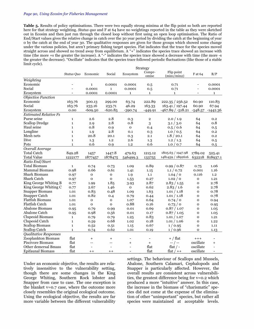
Page 90, Using Ecosim for Fisheries Management
Under an economic objective, the results are rela-tively insensitive to the vulnerability setting, though there are some changes in the King George Whiting, Southern Rock lobster and Snapper from case to case. The one exception is the blanket v=0.7 case, where the outcome more closely resembles the original ecological outcome. Using the ecological objective, the results are far more variable between the different vulnerability
settings. The behaviour of Scallops and Mussels, Abalone, Southern Calamari, Cephalopods and Snapper is particularly affected. However, the overall results are consistent across vulnerabili-ties, the greatest difference being for v=0.2 which produced a more “intuitive” answer. In this case, the increase in the biomass of “charismatic” spe-cies did not come at the expense of the elimina-tion of other “unimportant” species, but rather all species were maintained at acceptable levels.
Table 5. Results of policy optimisations. There were two equally strong minima at the flip point so both are reported here for that strategy weighting. Status quo and F at 64 have no weightings reported in the table as they were sketched out in Ecosim and then just run through the closed loop without first using an open loop optimisation. The Ratio of End/Start values gives the relative change in catch over the 30 year period by dividing the catch at the beginning of year 0 by the catch at the end of year 30. The qualitative responses are given for those groups which showed some change under the various policies, but aren’t primary fishing target species. Flat indicates that the trace for the species moved straight across and showed no trend away from equilibrium. A “+” indicates the species trace showed an increase with time (the more +s the greater the increase). A “-“ indicates the species trace showed a decrease with time (the more -s the greater the decrease). “Oscillate” indicates that the species trace followed periodic fluctuations (like those of a stable limit cycle). Strategy
Status Quo Economic Social Ecosystem Compr-omise
Flip point (min1/min2) F at 64 B/P
Weighting Economic - 1 0.0001 0.0001 0.5 0.71 - 0.0001 Social - 0.0001 1 0.0001 0.5 0.71 - 0.0001 Ecosystem - 0.0001 0.0001 1 1 1 - 1 Objective Function Economic 163.76 300.13 299.00 63.74 222.89 222.35 / 256.52 60.90 110.83 Social 163.76 233.16 233.71 46.29 163.33 163.41 / 197.44 60.90 67.94 Ecosystem 0.00 -609.50 -620.85 -390.74 -449.91 -467.89 / -518.21 -548.57 -1442.36 Estimated Relative Fs Purse seine 1 2.6 2.8 0.3 2 2.0 / 1.9 64 0.2 Scallop Dredge 1 2.9 2.8 0.8 3 3.1 / 3.0 64 0.8 Haul seine 1 0.8 0.9 0 0.4 0.5 / 0.6 64 0.5 Longline 1 1.9 2.8 0.1 0.3 1.0 / 0.5 64 0.2 Mesh nets 1 20.8 20.1 0.3 2.1 1.8 / 20.1 64 0.2 Dive 1 1.3 1.2 2.6 1.3 1.2 / 1.3 64 0.5 Pots 1 0.6 0.9 1.2 0.6 1.0 / 0.7 64 0.5 Overall Average Total Catch 849.28 1457 1447.8 479.63 1215.12 1805.63 / 1947.98 1789.02 525.41 Total Value 1222177 1877457 1878475 546499.3 133755 1481459 / 1892616 632218 818937.1Ratio End/Start Total Biomass 1 0.74 0.73 1.09 0.89 0.99 / 0.87 0.75 1.06 Mammal Biomass 0.98 0.66 0.61 1.41 1.15 1.1 / 0.72 0.001 1.16 Shark Biomass 0.97 0 0 1.9 1.1 1.04 / 0 0.116 1.2 Shark Catch 0.97 0 0 1.53 0.27 1.02 / 0 0 1.21 King George Whiting B 0.77 1.99 1.85 3.93 2.87 2.83 / 1.55 0 2.78 King George Whiting C 0.77 2.67 1.46 0 0.62 2.83 / 1.6 0 2.78 Snapper Biomass 1.01 0.83 0.48 1.09 1.63 1.01 / 1.18 0 0.78 Snapper Catch 1.01 0.82 0.4 0.79 0.44 1.01 / 1.18 0 0.78 Flatfish Biomass 1.01 0 0 1.07 0.64 0.74 / 0 0 0.94 Flatfish Catch 1.01 0 0 0.88 0.16 0.73 / 0 0 0.95 Abalone Biomass 0.95 0.79 0.99 0.01 0.69 0.87 / 1.07 0 1.05 Abalone Catch 0.95 0.98 0.56 0.01 0.17 0.87 / 1.05 0 1.05 Clupeoid Biomass 1 0.79 0.79 1.25 0.83 1.01 / 1.07 0 1.21 Clupeoid Catch 1 0.59 0.68 1.02 0.18 1.01 / 1.06 0 1.22 Scallop Biomass 1 0.52 0.51 1.15 0.67 1 / 0.95 0 1.11 Scallop Catch 1 0.74 0.62 1.01 0.19 1 / 0.96 0 1.13 Qualitative Responses Zooplankton Biomass flat + + - - + / flat +++ - Piscivore Biomass flat -- -- + + -- / -- oscillate + Other demersal Bmass flat - - - flat flat / - oscillate - Epifaunal Biomass flat ++ ++ - flat flat / ++ oscillate -

Fisheries Centre/FAO Workshop, Page 91
The conclusions from the sensitivity analyses are that the general policy analysis is fairly robust across vulnerability settings in this case, though the “standard economic solution” disappears at higher vulnerabilities. Furthermore, it is worth noting that oscillating output is very likely if the majority of the vulnerabilities are set at either ex-treme. At the lower end vulnerabilities it is really only an artifact of a mismatch in the numerical scheme used and the mean of the oscillations is trustworthy. At the higher end though it is the re-sult of chaotic dynamics and is thus often unin-terpretable. As with vulnerabilities, policy outcomes seem relatively insensitive to minor changes in the various ecological importance criteria. It was found that abalone are no longer eliminated when some importance is placed on its retention in the system. One notable feature of the PPB Ecosim model is the relative lack of responsiveness at lower tro-phic levels. This contrasts with other trophic models being developed for the PPB system. To
test whether such responsiveness could be “forced” within Ecosim, one scenario examined the consequences of increasing the Fs on all fisheries to 64 times their current levels. Not sur-prisingly, all the fish groups were rap-idly depleted, but there was still very little response in the lower trophic lev-els. This may be due to the amount of “leeway” in the EE values for the pri-mary producers in the system (as little as 0.6), as they are feeding the domi-nant detrital foodweb rather than the classic, primary producer based, foodweb in this system. The introduc-tion of a dummy fleet that fishes zoo-plankton and detritivores detritivores could allow some exploration of this is-sue. Discussion For the Port Phillip Bay model exam-ined in this study, there are three char-acteristic system responses corre-sponding to three possible policy ob-jectives. These can be best summarized using the sharks as an indicator spe-cies: 1. Economic objectives are dominant: sharks are removed from the system; 2. Compromise of economic and ecological objectives: sharks persist at current levels; 3. Ecological objectives are dominant: sharks allowed to increase.
The fact that these results are so consistent across parameter settings, and that most of the ancillary groups are so unresponsive under the different objectives, highlights a few interesting points. The first of these is that in this study sharks act as a very good indicator species for both system re-sponse and policy objectives. Choice of ecological indicators has become a very important topic re-cently. Identifying a species or group that is sensi-tive to system changes and which is a useful measure of policy performance would prove very useful, both within model studies and in field monitoring. The second point raised by the results of the pol-icy analysis is that the modelled system is fairly insensitive, with some pools showing no change even under extreme changes, such as F at 64 times current levels. This suggests either that the model itself is insensitive to change, and that some structural exploration may be of use, and/or that the system itself is robust to change as it is
Figure 2 – Biomass through time plots for the optimisation under primarily economic objective.

Page 92, Using Ecosim for Fisheries Management
built primarily upon a detritus based foodweb rather than a classical web. Simulations from an-other dynamic model program suggest that Port Phillip Bay is much more strongly affected by eu-trophication than by fishing, and this may explain and support the insensitivity of the lower trophic groups in the Ecoosim simulations run here. Ei-ther way, more research into the form and basis of the foodwebs in Port Phillip Bay, especially the pelagic ones, would be instructive in evaluating how well the Bay might cope with increasing pres-sures. Lastly, an important cautionary note. The lack of cost data for the fisheries meant that the eco-nomic objectives really only used the value of the fisheries to determine the outcome. The inclusion of reliable and realistic cost data may well see dif-ferent or at least a wider range of results and is an exercise that will be completed in the near future. General conclusions Vulnerabilities are one of the most crucial ele-ments of Ecosim and their potential effect on pol-icy evaluations can not be neglected. Ecosim’s best performance (with regard to matching real-ity) is most often seen when higher trophic levels or heavily depleted groups have high prey vulner-abilities and lower trophic levels have v in the range 0.4 to 0.5. Furthermore, even though vul-
nerabilities generally had little qualitative effect on the overall outcome of the policy evaluations in this case, it was apparent that the choice of vulnerability settings may prove to be crucial in other circumstances and so must be given a good deal of attention. For instance if we had been con-cerned more with a particular species, say aba-lone, rather than the system as a whole then vul-nerabilities and their effect on policy evaluation may have had a much more striking impact here. The criteria used to determine management ob-jectives must also be carefully considered. Eco-nomic and social objectives may lead to radical restructuring of ecosystems unless they are bal-anced with some ecological reference points. However, conservation and public pressure to preserve charismatic species may not, in fact probably will not, lead to balanced ecosystems. Some measure of importance must be given to all groups in the system if a balanced, ecologically robust system is to result from management pol-icy implementation. References Anon, 1996. Catch and Effort Information Bulletin
1995. Conservation and Natural Resources: Victo-rian Fisheries Research Institute: Queenscliff, Vic-toria, Australia.
Beattie, G., A. Redden and R. Royle 1996. Microzoo-plankton Grazing on Phytoplankton in Port Phillip
Figure 3 – Biomass through time plots for the op-timisation under primarily ecological objective.
Figure 4 – Biomass through time plots for the com-promise, or first step change, optimisation
Fisheries Centre/FAO Workshop, Page 93
Bay. Technical Report No. 31. Port Phillip Bay En-vironmental Study. CSIRO: Canberra, Australia.
Briggs, K.T., W.B. Tyler, D.B. Lewis, D.B. and D.R. Carlson 1987. Bird Communities at Sea off Califor-nia: 1975-1983. Studies in Avian Biology. 11.
Dolphin Research Institute 2000. Dolphin Education Project Question and Answers. Dolphin Research Institute: Frankston, Victoria, Australia. Also available at http://www.dolphinresearch.org.au/institute.html
Gunthorpe, L., P. Hamer and S. Walker 1997. Bays and Inlets Scalefish Fisheries Review: Volume 1: Life cycles and habitat requirements of selected Victo-rian fish species, including an assessment of the main habitat threatening processes and recom-mendations for habitat maintenance, rehabilita-tion and enhancement. Marine and Freshwater Resources Institute: Queenscliff, Victoria, Austra-lia.
Hall, D.N. (ed), 1992. Port Phillip Bay Environmental Study: Status Review. Technical Report No. 9. Port Phillip Bay Environmental Study. CSIRO: Can-berra, Australia.
Harris, G., G. Batley, D. Fox, D. Hall, P. Jernakoff, R. Molloy, A. Murray, B. Newell, J. Parslow, G. Skyring and S. Walker 1996. Port Phillip Bay Envi-ronmental Study Final Report. CSIRO: Canberra, Australia.
Holloway, M., and G. Jenkins 1993. The Role of Zoo-plankton in Nitrogen and Carbon Cycling in Port Phillip Bay. Technical Report No. 11. Port Phillip Bay Environmental Study. CSIRO: Canberra, Aus-tralia.
Kailola, P.J., M.J. Williams, P.C. Stewart, R.E. Reichelt, A. McNee and C. Grieve 1993. Australian Fisheries Resources. Bureau of Resource Sciences, Depart-ment of Primary Industries and Energy and the Fisheries Research and Development Corporation: Canberra, Australia.
Lee, P.G. 1994. Nutrition of Cephalopods: Fueling the System. Marine Behaviour and Physiology. 25 (1-3): 35-51.
Murray, A., and J. Parlsow 1997. Port Phillip Bay Inte-grated Model: Final Report. Technical Report No. 44. Port Phillip Bay Environmental Study. CSIRO: Canberra, Australia.
Nicholson, G.J., A.R. Longmore and R.A. Cowdell 1996. Nutrient Status of the Sediments of Port Phillip Bay. Technical Report No. 26. Port Phillip Bay En-vironmental Study. CSIRO: Canberra, Australia.
Officer, R.A., and G.D. Parry 1996. Food Webs of Demersal Fish in Port Phillip Bay. Technical Re-port No. 36. Port Phillip Bay Environmental Study. CSIRO: Canberra, Australia.
Parry, G.D., D.K. Hobday, D.R. Currie, R.A. Officer and A.S. Gason. The Distribution, Abundance and Di-ets of Demersal Fish in Port Phillip Bay. Technical Report No. 21. Port Phillip Bay Environmental Study. CSIRO: Canberra, Australia.
PICES Working Group 11 1998. Consumption of Ma-rine Resources by Marine Birds and Mammals in the PICES Region. 1998 Report of Working Group 11. Sidney, Canada. Also available at http://pices.ios.bc.ca/wg/wgf.htm.
Poore, G.C.B. 1992. Soft-bottom macrobenthos of Port Phillip Bay: a literature review. Technical Report
No. 2. Port Phillip Bay Environmental Study. CSIRO: Canberra, Australia.
Schmid, T. H., F.L. Murru and F. McDonald 1993. Feeding habits and growth rates of bull (Carchari-nas leucas), sandbar (Carcharinas plumbeus), sandtiger (Eugomphodus taurus), and nurse (Ginglymostoma cirratum) sharks. Journal of Aquaculture and Aquatic Sciences 5(4): 100-105.
Wilson, R.S., B. F. Cohen and G.C.B. Poore 1993. The Role of Suspension-feeding and Deposit-feeding Benthic Macroinvertebrates in Nutrient Cycling in Port Phillip Bay. Technical Report No. 10. Port Phillip Bay Environmental Study. CSIRO: Can-berra, Australia.
Page 94, Using Ecosim for Fisheries Management
Simulating extreme fishing polices in Prince William Sound, Alaska: a preliminary evaluation of an ecosystem-based policy analysis tool Thomas A. Okey Fisheries Centre, UBC Abstract The biotic assemblage of Prince William Sound, Alaska has changed considerably during the last 35 years in re-sponse to the great Alaskan earthquake, oceanographic changes, fisheries activities, the Exxon Valdez oil spill, and other factors. The multifactorial nature of the mechanisms of change in this system make it challeng-ing to discern their relative importance when attempt-ing to understand troublesome trends. The manage-ment of fisheries stands out, however, as a way of shap-ing the state of living marine resources because fisher-ies are controllable and they influence biotic assem-blages. A new dynamic simulation tool in Ecopath with Ecosim enables comparisons of various fishing policy scenarios in a whole food web context according to dif-ferent weightings of ‘economic,’ ‘social’ (employment), and ‘ecological’ considerations. A simplistic exercise in which a policy compromise was developed from three extreme polices—corresponding with optimization of these three objectives—enabled comparison of the find-ings among systems featured in this volume. Optimiza-tion of short-term economic goals and social (employ-ment) goals in Prince William Sound led to simulated fishing strategies that caused direct, fishery-imposed extinction of top predators (e.g., pinnipeds, Pacific halibut, and lingcod), resulting in increases in bio-masses of two gadoid species (Pacific cod and sable-fish), and thus the overall monetary and employment value of the system. Such a strategy of imposing extinc-tions to optimize short-term economic or employment value is generally illegal, though perhaps operational in some systems throughout the world. Optimization of ecological considerations led to fishing scenarios that increased porpoise, pinnipeds, orcas, seabirds, and other high trophic level predators, while correspond-ingly decreasing the same two gadoid species. The po-tential importance of direct take of pinnipeds, as well as food competition between fisheries and other high trophic level species, is indicated by positive responses of these groups to decreases in fishing, though this simulated response does not imply that other sources of stress and mortality are unimportant to apex preda-tors. The numerical stability of pinnipeds (the chosen assessment endpoint) was achieved by weighting the ecological considerations by a factor of 3.2 over eco-nomic and social considerations. Predicted reductions in catches by subsistence, recreational, and commercial fisheries by the end of all 20 year simulations were thought to be a function of discounting the future dur-ing the policy search procedure through initially-aggressive value optimization, though it may also be an indication that current fishing exceeds sustainable lev-
els in an ecosystem context. Predicted catch reductions associated with the weighted compromise were not considerably different than catch reductions associated with other options. Introduction Prince William Sound (PWS) is a coastal marine embayment situated at the northern apex of the Gulf of Alaska, north of latitude 60° (longitude 146° W). Its area covers just over 9,000 km2, or approximately 15 San Francisco Bay units. The ecological uniqueness of Prince William Sound is due largely to the interplay of its physical charac-teristics with the climatic and oceanographic characteristics of the region. Warm moist air ar-riving from the south becomes trapped, uplifted, and cooled by the surrounding Chugach Moun-tains, releasing considerable precipitation. An-nual rainfall ranges from 160 to 440 cm in PWS, and snowfall can reach 2290 cm in the surround-ing mountains (Michelson 1989 in Wheelwright 1994). Rain runoff and snowmelt enter from myr-iad streams, but icebergs and glacial melt also contribute fresh water. Yet greater amounts of fresh water enter PWS as a stratified lens aloft an incurrent of marine water at the Hinchenbrook entrance. Numerous rivers and glaciers feed this freshwater lens as it is transported alongshore by the Alaska coastal current from as far south as British Columbia (Wheelwright 1994). Complex estuarine gradients and interfaces are present. The Sound’s highly variable depths (800 m maximum and 300 m mean; Cooney 1993, Loughlin 1994) relate to its origins as a sub-merged section of the formidable Chugach Moun-tains, which surround and frame it. The habitats of the sound are relatively isolated from the Gulf of Alaska by barrier islands and two relatively narrow channels. Its coastline is very convoluted, and in many places it drops off steeply just be-yond a narrow shelf. Other parts of the sound contain extensive shallow areas, and still others drop vertically as the subaerial walls of fjords. Although organisms inhabiting Prince William Sound are reasonably typical of sub-polar coastal marine environments, the biotic community is shaped by the ecosystem’s unique physical attrib-utes. Examples include protection from outer coast wind and waves, estuarine gradients, is-lands and heterogeneous coastlines, large inter-tidal zones (e.g., diurnal tide range at Cordova = 3.8 m; NOAA 1984), rocky habitats, mudflats, cobble beaches, steep and short spawning streams, fjords and their associated glaciers and turbidity gradients, and extreme physical season-

Fisheries Centre/FAO Workshop, Page 95
ality. All of these combine to produce a unique and productive environment for diverse assem-blages of marine mammals, birds, invertebrates, fishes, plants, and microorganisms. Longer-term climatic oscillations have also influenced the abundances of some species in the region, such as salmon (NRC 1996, Mantua et al. 1997). Humans began interacting with the biota of the Prince William Sound ecosystem approximately 10-15 thousand years ago, soon after crossing the Bering Straight (Dumond and Bland 1995). The ecological influence of these first residents of the region is not well known, though they likely col-lected clams from the intertidal and shallow ar-eas, salmon from the many streams and rivers (Cooley 1961), marine mammals (e.g., Simenstad et al. 1978), and other fishes, invertebrates, sea-birds, and marine algae. The first modern impacts to the region’s marine ecosystem came over two centuries ago when Russian traders and furriers hunted the newly discovered Steller’s sea cow (Hydrodamalis gigas) to biological extinction and the sea otter (Enhydra lutris) to ecological extinc-tion. The removal of the sea otter undoubtedly triggered considerable changes in nearshore zones, as this species is known to exert strong keystone effects throughout its still expanding range (Estes and Palmisano 1974, Estes et al. 1974, Dayton 1975, Simenstad et al. 1978, Kvitek et al. 1992, Estes and Duggins 1995). The ecologi-cal changes caused by the extinction of the Steller’s Sea Cow will remain in the realm of speculation (e.g. Pitcher 1998). Although the activities of 20th century Alaskan fishing industries are reasonably well recorded, their broader ecological effects are poorly known, as the complexity of these ecosystems prevented our understanding of whole food web dynamics. Industrial whaling targeted baleen whales be-tween 1845 to 1966, but much of the whale bio-mass was removed in the final years of that fish-ery. It has been suggested that the removal of a large proportion of the baleen whales in Alaskan waters triggered cascading effects such as in-creases in gadoid fish (e.g., through a release in foraging competition between juvenile pollock and whales; see NRC 1996). Offshore foreign fleets removed considerable proportions of Pacific herring populations from Alaskan waters during the first three decades after WW-II. Catches peaked in 1970 at over 140,000 t⋅year-1, then quickly declined by an order of magnitude (Ja-cobson et al.1999). Pacific herring shows signs of gradual recovery in all Alaskan regions except for Prince William Sound where runs failed to return four years after the Exxon Valdez oil spill. Pacific herring is of primary commercial importance in
PWS, and it is an important forage fish for higher trophic levels. Slope rockfish, particularly Pacific Ocean perch, were likewise heavily exploited in the Gulf of Alaska region during the 1960s. They remain at low levels, but are said to be responding to conservative management (Low et al. 1999). Major changes have occurred in the PWS ecosys-tem during the last 20 years. Red king crab and shrimp populations collapsed, and their fisheries were closed with no signs of recovery (Reeves and Turnock 1999); pinnipeds, including harbor seals and sealions have declined steadily (e.g., Frost et al. 1998); and some seabirds, such as common murres, cormorants, and black legged cormorants have declined—all since the early 1980s (EVOS 2000). In contrast, fish species such as Pacific cod, walleye pollock, and flatfish have increased considerably in the region during this same time period. Alaskan groundfish fisheries are fully util-ized and overcapitalized, and the associated by-catch of king crabs, shrimp, herring, and snow crabs may hinder the recovery or the resilience of these formerly abundant species (Low et al. 1999). All species of salmon have increased con-siderably during this time period. Although sev-eral salmon hatcheries in Prince William Sound contribute to a large proportion of the pink salmon captured in the local fisheries, increased adult survival in the Alaska Gyre is the most likely reason for the record salmon runs in recent years (Wertheimer 1997, Heard and Anderson 1999). The notion that shifting oceanographic conditions in the region strongly influences the region’s ma-rine community structure and is associated with some of the observed changes now holds consid-erable weight (Hollowed and Wooster 1992, Brodeur et al. 1996, Piatt and Anderson 1996, Ty-ler and Kruse 1996, Francis et al 1998, Rosenk-rantz 1999). Fisheries can, nevertheless, exacerbate climate-driven fluctuations by changing the resiliencies of populations to natural disturbance or stress (sensu Holling 1973, Sousa 1984). Insight into these influences can be gained by examining the potential forcing caused by fisheries in a system-wide, interaction-web context. Furthermore, evi-dence is continuing to mount that high trophic level predators, such as mammals and birds, can be adversely affected by intensive fisheries at lower trophic levels (e.g., Mackinson et al. 1997, Springer and Speckman 1997). Trites and his col-leagues (1997), on the other hand, suggest that competition for food by fisheries does not gener-ally have important detrimental effects on marine mammals, based on evidence that diet overlap is small between fisheries and marine mammals. The relative importance of such competition and

Page 96, Using Ecosim for Fisheries Management
detrimental effects undoubtedly varies among ecological setting, and this question has far-reaching implications for both fisheries and ma-rine biota. There is also no question that design-ing policy and analyses around the question of human-nonhuman competition will be con-strained by conservation laws and subsistence-
rights laws. Most of the approximately 7,000 people in Prince William Sound reside either in the two Alaska Na-tive villages, Chenega Bay and Tatitlek, or the three larger communities Cordova, Valdez, and Whittier, two of which include Alaska Native vil
Table 1. Basic input parameters and detritus fate for the Prince William Sound model, 1994-1996. TL = trophic level cal-culated by Ecopath; OI = omnivory index indicating the degree of omnivory; P/B = production/biomass; Q/B = consump-tion/biomass; EE = ecotrophic efficiency, expressing the proportion of the production lost to export or predation. Detritus fate is a percentage allocation of the remaining production between detritus pools. (Nekton fall = dead carcases to sea floor.) Values in italics/light shading were calculated by Ecopath; other values are empirically-based input estimates, con-tributed by a collaboration of experts on PWS (Okey and Pauly 1999a).
Detritus fate (%) Group
Trophic
level
OI
Biomass (t⋅km-2)
P/B
(year-1)
Q/B
(year-1)
EE Nekton
fall In-
shore Off-shore Export
Transient Orca 5.4 0.01 0.001 0.05 6.04 0 1 - 50 49 Resident Orca 4.9 0.21 0.015 0.05 8.67 0 1 - 50 49 Sharks 4.5 0.98 0.662 0.10 7.00 0.753 1 - 99 - Halibut 4.5 0.36 0.677 0.32 1.73 0.865 1 - 99 - Porpoise 4.5 0.20 0.015 0.24 29.20 0.989 1 30 69 - Pinnipeds 4.4 0.15 0.072 0.06 25.55 0.994 1 30 69 - Lingcod 4.3 0.35 0.077 0.58 3.30 0.816 - 40 60 - Sablefish 4.0 0.87 0.293 0.57 6.42 0.774 - - 100 - Adult flounder 4.2 0.12 4.000 0.22 3.03 0.792 - - 100 - Adult salmon 4.2 0.05 3.410 1.31 13.00 0.996 - 30 - 70 Pacific cod 4.1 0.47 0.300 1.20 4.00 0.936 - - 100 - Juv flounder 4.0 0.12 0.855 0.22 3.03 0.956 - - 100 - Avian raptors 3.9 2.07 0.002 0.05 36.50 0.000 - 25 - 75 Seabirds 3.8 0.54 0.022 0.17 150.60 0.976 - 40 40 20 Deep demersals 3.8 0.80 0.960 0.93 3.21 0.984 - - 100 - Pollock 1+ 3.8 0.24 7.480 0.71 2.56 0.998 - - 100 - Rockfish 3.7 0.26 1.016 0.17 3.44 0.969 - 20 80 - Baleen whales 3.7 0.16 0.149 0.05 10.90 0 1 - 99 - Juv. salmon 3.5 0.31 0.072 3.91 62.80 0.969 - 30 70 - Nearshore demersal 3.3 0.24 4.200 1.00 4.24 0.776 - 100 - - Squid 3.3 0.01 3.000 3.00 15.00 0.940 - - 100 - Eulachon 3.2 0.63 0.371 5.00 18.00 0.991 - 40 20 40 Sea otters 3.2 0.18 0.045 0.13 117.00 0.005 - 50 50 - Deep epibenthos 3.2 0.62 30.00 3.00 10.00 0.961 - - 100 - Capelin 3.1 0.02 0.367 3.50 18.00 0.999 - 50 30 20 Adult herring 3.1 0.01 2.810 1.54 18.00 0.962 - - 100 - Pollock 0 3.1 0.01 0.110 2.34 16.18 0.945 - 50 50 - Shal large epibenth. 3.1 0.03 3.100 2.10 10.00 0.750 - 80 20 - Sea ducks 3.1 0.00 0.005 0.20 450.50 0 - 40 40 20 Sandlance 3.1 0.01 0.595 2.00 18.00 0.946 - 50 50 - Juv. herring 3.0 0.01 13.406 0.73 18.00 0.985 - 30 70 - Jellies 3.0 0.11 6.390 8.82 29.41 0.004 - 10 90 - Deep small infauna 2.3 0.23 49.400 3.00 23.00 0.916 - - 100 - Near omni-zoo 2.3 0.19 0.105 7.90 26.33 0.982 - 70 30 - Omni-zooplank 2.3 0.19 24.635 11.06 22.13 0.979 - 10 90 - Shal small infauna 2.2 0.18 51.500 3.80 23.00 0.941 - 100 - - Meiofauna 2.1 0.11 4.475 4.50 22.50 0.950 - 20 80 - Deep large infauna 2.1 0.09 28.350 0.60 23.00 0.931 - - 100 - Shal small epibent 2.1 0.05 26.100 2.30 10.00 0.976 - 70 30 - Shal large infauna 2.0 0.00 12.500 0.60 23.00 0.520 - 100 - - Near herbi-zoo 2.0 0.00 0.136 27.00 90.00 0.978 - 70 30 - Herbi-zooplankt 2.0 0.00 30.00 24.00 50.00 0.976 - 10 90 - Nearshore phytopl 1.0 0.00 5.326 190.00 - 0.950 - 70 30 - Offshore phytopl 1.0 0.00 10.672 190.00 - 0.950 - 10 90 - Macroalgae & grass 1.0 0.00 125.250 4.00 - 0.135 - 50 50 - Nekton falls 1.0 0.21 2.000 - - 0.953 - 80 20 - Nearshore detritus 1.0 0.30 19.520 - - 0.542 - - 100 - Offshore detritus 1.0 0.46 114.480 - - 0.587 - - - 100
Fisheries Centre/FAO Workshop, Page 97
lage corporations. All of these communities rely on commercial fishing, though the native villages conduct subsistence fishing and gathering. In ad-dition, Whittier is a growing hub of sportfishing activities, especially with the opening of a new road directly from Anchorage—Alaska’s largest city. Much of the economy of Valdez relies on the southern terminus of the trans-Alaska pipeline where supertankers are loaded with oil for trans-port across the Gulf of Alaska and beyond (EVOS 2000). Considerable changes imposed on subsis-tence, commercial, and recreational fisheries, are related not only to the population fluctuations mentioned previously, but also due to a crash in the market value of wild salmon triggered by salmon farming (Folsom et al. 1992), and due to the catastrophic Exxon Valdez oil spill (see Picou et al. 1997). The supertanker T/V Exxon Valdez ran aground on Bligh Reef in Prince William Sound causing the largest oil spill in United States history (over 40 million liters of crude oil). The oil spread throughout central and southwestern PWS, into the Gulf of Alaska, along the Kenai Peninsula, into Cook Inlet, to Kodiak Island, and along the Alaska Peninsula (see Figure 2 in Paine et al. 1996). The initial effects of the oil spill were catas-
trophic, killing several hun-dred thousand seabirds and other birds of 90 species; 3,500-5,500 sea otters; 1,000 bald eagles, 10% of the world’s population of the threatened Kittlitz’s mur-relet; a number of killer whales; 300 harbor seals, other marine mammals; and vast numbers of fish, inver-tebrates, and plants (Lough-lin 1994, Paine et al. 1996, Spies et al. 1996). Although the spill’s full acute effects will remain uncertain, there is little doubt that they cas-caded and reverberated through the impacted sys-tems in addition to operat-ing directly and immedi-ately. Even more uncertain than initial impacts are questions of recovery, resil-iency, and long-term effects (see Okey et al., in prep.a). A mass-balance model of the post-spill Prince William Sound food web (1994-1996) was constructed, re-
fined, and disseminated during 1998 and 1999 (Okey and Pauly 1999a). The PWS model is avail-able for downloading at no charge with the latest Ecopath with Ecosim software from www.ecopath.org, the derivations of its parameters are fully documented in Okey and Pauly (1999b), and the emergent characteristics of the model are described in greater detail in Okey et al. (in prep.a). In addition, a CD ROM containing the model and other Alaska resources is available (Okey et al. 2000). The basic parameters for the Prince William Sound model are shown in Table 1. The basic in-put parameters production/biomass (P/B) and consumption/biomass (Q/B) are expressed in an-nual units. The ecotrophic efficiency (EE) is the proportion of production by a group consumed by predators or lost to export. This ratio, along with trophic level (TL) and omnivory index (OI), is cal-culated by the Ecopath formulation for each spe-cies. Detritus fate is a percentage allocation among detritus pools of the unconsumed and unexported production of a group. Values in bold were calculated by Ecopath; values not bolded are empirically-based input estimates contributed by a collaboration of experts on PWS, or estimates that were modified to achieve thermodynamic
Table 2. Estimates of mean annual fishery landings and discards in Prince Wil-liam Sound (1994-1996).
Landings (t⋅km-2⋅year-1)
Dead discards (t⋅km-2⋅year-1)
Group Com-
merciala Recrea-tionalb
Subsis-tence
Com-mercial
Recrea-tionalg
Adult salmon 5.3726 - 0.0002 - - Adult Pacific herring 2.5455 - - 0.0551e - Pollock 1+ 0.1710 - - 0.0103f - Deep epibenthos 0.1430 - - - - Shallow demersals 0.0700 - - 0.0001 - Pacific cod 0.0656 - - 0.0016 - Pacific halibut 0.0268 0.0423 - - 0.0015 Sablefish 0.0184 - - 0.0008 - Rockfish 0.0060 0.0039 - 0.0005 0.0020 Shallow large infauna 0.0030 - - - - Adult arrowtooth flounder 0.0004 - - 0.0019 - Deep demersal fishes 0.0003 - - 0.0023 - Sharks 0.0003 - - 0.0022 0.0019 Lingcod 0.0003 0.0023 - - 0.0002 Juv. arrowtooth flounder 0.0001 - - 0.0019 - Juv. Pacific herring - - - 0.1189 - Pinnipeds - - 0.0020 - - Totals 8.4234 0.0485 0.0022 0.1958 0.0037 a) adapted from commercial landings from B. Bechtol (ADF&G, unpublished data) b) from Meyer (1999) c) from Morestad et al. (1997) d) from Frost (1999) e) based on ballpark estimates by J. Wilcox, ADF&G (pers. comm., 25 Oct 1999) f) based on postal surveys by Howe et al. 1995-1997 g) group-specific discard ratios calculated from data provided by M. Furuness, NMFS
these ratios were applied to PWS landings data provided by B. Bechtol, AKF&G h) from Hukbert (1999)

Page 98, Using Ecosim for Fisheries Management
balance of the groups and the model (Okey and Pauly 1999a, b). The estimates of mean annual fishery landings and discards in Prince William Sound between 1994 and 1996 shown in Table 2 were used as inputs in the PWS model. Monetary values per unit of species captured by the fisher-ies were also input to the PWS model for the “economic” valuation in this analysis (Table 3). Commercial ex-vessel values are from Frenette et al. (1997) and these were multiplied by 10 in or-der to derive values for recreationally captured fishes (as suggested by C. Walters, UBC Fisheries Centre, pers. comm., 20 July 2000). The esti-mated substance value of pinnipeds used here ($8.50⋅kg-1) is the sum of the given edible value ($5⋅kg-1 of seal), the hide value ($2⋅kg-1 of seal), and the craft value ($1.50⋅kg-1 of seal)(K. Frost, ADFG, pers. comm., 10 Aug 2000). The commer-cial value of salmon was also used as the sub-stance value of salmon. A balanced trophic model of the Prince William Sound food web has been constructed using the Ecopath with Ecosim approach, but confusion ex-ists among potential model users and decision-makers in Alaska about the nature of the ap-proach and its degree of usefulness for practical fisheries management and planning. Dynamic simulation routines allowing exploration of the potential indirect effects of specified changes in fishing (or disturbance) are now supplemented with a suite of analytical tools for fishery policy
analysts. These new tools are designed to explore the potential effects and success of management policies on economic, social, and ecological re-sources (Walters, this volume). Application of this approach to the Prince William Sound model is presented here as a simplistic and preliminary ex-ercise to evaluate the efficacy of this approach for the future planning of Alaska’s fisheries. The cur-rent analysis is simplistic because the contrasted policies are intended to represent the extremes of “economic,” “social,” and “ecological” objectives as defined by the author, for ease of comparison among different systems (this volume), and be-cause the current version of the Prince William Sound model explicitly identifies only three broad fisheries categories: subsistence, recreational, and commercial, rather than individual gear types. Methods A comparison of hypothetical policies that opti-mize ‘economic’, ‘social’, and ‘ecological’ consid-erations necessitates definitions of these terms that are unavoidably arbitrary to some extent. The first problem is with the concept of ‘econ-omy.’ If ‘economy’ is defined as a system or pat-tern of resource flow, and the goal of economic endeavors is the “thrifty use of resources” (Mer-riam-Webster 1995), then optimization of eco-nomic goals on the broadest time scale and tro-phic scales would lead to the application of nega-tive discount rates (natural capital would be con-sidered to increase in value over time). A broad definition of economy would also lead to a valua-tion of ecosystem services that converges with, rather than contrasts with, ecologically-based valuations. However, the economic/electoral sys-tem in the United States and throughout most of the world emphasizes decisions that maximize short-term individual self-interest, rather than broader scale and longer-term self interests. In order to contrast “economic” with the other two objectives, then, the operational concept of short-term economic interests is used here in place of the inherently broader concept of ‘economic in-terests.’ Social considerations encompass a wide spectrum of connections between human and natural com-munities of Prince William Sound. Because most these aspects are impossible to quantify for the purposes of comparative analysis, one single as-pect of social considerations — employment value — is used here as a proxy for this complex realm. Employment value is defined here as number of jobs per captured unit of a particular biotic group that is targeted by a fishery.
Table 3. Economic values assigned to exploited PWS groups.
Economic values of PWS animals ($⋅kg-1)
Group Name Subsis-tencea
Recrea-tionalb
Comm-ercialc
Halibut - 60.10 6.01 Lingcod - 39.10 3.91 Rockfish - 39.10 3.91 Pinnipeds 8.50 - - Deep epibenthos - - 5.38 Sablefish - - 3.91 Adult arrowtooth - - 3.91 Pac. Cod - - 3.91 Juvenile arrowtooth - - 3.91 Deep demersals - - 3.91 Pollock 1+ - - 3.91 Nearshore demersals - - 3.91 Adult salmon 3.75 - 3.75 Adult herring - - 2.49 Shallow large infauna - - 2.12 a. The valuation of pinnipeds was based on figures provided by
K. Frost, ADFG, pers. comm., 10 Aug 2000 b. Recreational and sport fish values were considered to be an
order of magnitude more valuable than commercial values (C. Walters, UBC Fisheries Centre, pers. comm., 20 July 2000)
c. Calculated from landings and ex-vessel values provided by Frenette et al. (1997)

Fisheries Centre/FAO Workshop, Page 99
The quantification of ecological considera-tions for comparison to short-term eco-nomic and employment considerations also presents a potentially challenging di-lemma. One approach is to attempt mone-tary valuation of natural capital, based on ecosystem services and utilitarian as-sumptions (e.g., Costanza et al. 1997). However, a less value-laden approach is to use inherent biological properties to opti-mize particular qualities of interaction webs. Following this approach, the inverse of the ratio of production to biomass was used as a weighting factor to optimize food web structure and ecological quality, as it was considered to be a meaningful ecological property. This weighting factor (1/(P/B)) gives higher weight (“impor-tance”) to slower-growing and longer-lived species in the system’s interaction web, thus favoring ‘K-selected’ species. This would, in theory, maximize the number of trophic levels possible in the system and optimize the overall trophic transfer efficiency. Fishing strategies that lead to such ecological reconstruc-tion would amount to ‘fishing the food web back up,’ rather than ‘fishing down the food web’ (Pauly et al. 1998). Given this structure-based definition, ecological considerations are here la-beled ‘ecosystem structure.’ After developing the operational definitions of these three basic objectives, the policy search simulations were set up in Ecosim by conducting the following steps in addition to checking the appropriateness of default settings. The four spe-cies in the model containing explicitly separated ontogenetic stages were linked in the ‘stage’ inter-face, and the parameters specifying the character of their linkage were scrutinized. The prey vul-nerabilities were specified to one of the three vul-nerabilities used in this exercise (0.2, 0.4, and 0.7). These specify the relative importance of top-down vs. bottom-up forces influencing each in-teraction. They can be set for individual interac-tions, but one of the three settings was applied to the whole system for each of the three ‘sensitivity’ variants of each scenario. Although the five apex predators in the system as well as birds, Pacific herring, salmon, and lingcod exhibited dramatic positive biomass responses to scenarios in which ecological considerations were optimized, Pinnipeds proved to be the most sensi-tive biological component of the Prince William Sound model with respect to declines and extinc-tion responses. For this reason, the pinniped group, which consists mainly of harbor seals (Phocenia phoca) in Prince William Sound, was
chosen as the ecological endpoint for develop-ment of the weighted compromise of the more simplistic simulations. Numerical stabilization of harbor seal biomass was used as the assessment endpoint, and various policies were explored around that goal. Fishing restrictions estimated from this goal would represent the minimal that would be necessary to protect pinnipeds in Prince William Sound for two reasons: (1) the simula-tions assume a pinniped population in equilib-rium rather than accounting for the currently ob-served decline in the PWS harbor seal population, and (2) the numerical stabilization goal does not account for any rebuilding of the harbor seal population that might be deemed appropriate. However, indicated restrictions in fishing are simplistic because of the broad categories of fish-ing that are used, and population responses to limits in fishing could mean either direct or indi-rect effects of fishing levels imposed by Ecosim, thus revealing only the potential for such re-sponses in the system. The ‘non-linear search procedure for optimum fishing strategy over time’ was prepared for each scenario (e.g., Figure 1). Each search was started at the base fishing mortalities specified in the 1994-1996 PWS Ecopath model. The search was run using the Fletch method; and the annual eco-nomic discount rate was kept at 0.04 for all simu-lations. The objectives (“economic,” employment, and ecological) were defined by entering their quantitative definitions (see above) into the Eco-sim interfaces provided for employment and eco-logical definitions (“economic” considerations are defined by local market values of captured species specified in the Ecopath model; Frenette et al. 1997). Each search was then run according to the
0.1
10
4 27 52 79 114 154
Evaluation stepsRela
tive
fishi
ng
SubsistenceRecreationalCommercial
Figure 1. An example of a search for optimum beginning catch rates relative to 1994-1996 Prince William Sound catch rates, here for the weighted compromise scenario. This procedure finds the ideal starting catch rates for each fishing category based on the specified parameters. The ending values shown here are used as the starting values for the 20-year dynamic policy simulation

Page 100, Using Ecosim for Fisheries Management
optimized objec-tive. In these ex-treme simula-tions, the opti-mized objective was given a value of 1.0 while the remaining two were given values of 0.0001. All three objectives were set at 1.0 in the simple com-promise scenario, and then multiple searches were conducted to find the values that achieved the assessment endpoint. The scenario that achieved the assessment end-point was used as the weighted compromise. These searches for optimal fishing patterns over time (according to specified objectives) resulted in initial fishing levels that were considerably dif-ferent from those in Prince William Sound be-tween 1994 and 1996. For example, the new ‘starting’ fishing rates for these hypothetical 20-year simulations contrasted profoundly with the actual (1994-1996) rates (Figure 2). Starting with these new fishing strategies, which solved for the constraints imposed by the defined objectives, the simulations were run in ‘closed loop’ mode to simulate the dynamic interplay be-tween fishery managers and all the biotic compo-nents of the food web. The results of these simula-tions were recorded by transferring run results onto spreadsheets. Predicted changes in relative biomass levels for the four main simulations (by the end of 20 year runs) were plotted, as were predicted changes in catches by the three fisheries categories, for each optimization scenario. These resulting values of each of the three objectives were then compared to values resulting from ‘open loop’ simulations in which no management error exists. This is further explained below.
Walters (this volume) asks us to imagine a fishery manager who has perfect knowledge of the sys-tem, and can instantaneously make perfect man-agement decisions in the context of goals we have specified be optimized. For each scenario, this hypothetical manager-demon can optimize speci-fied values of living resources while losing none of that value to uncertainty or managerial fallibility. The resulting values from these perfect ‘open-loop’ simulations are then compared with the val-ues resulting from the dynamic ‘closed loop’ simulation in which information and manage-
ment decisions are simulated to be imperfect. Al-though the formulation of this imperfectness is it-self imperfect in Ecosim, it is imperfect in a con-sistent way such that this method can be used to compare fishing categories and optimization sce-narios. Finally, the mean of the relative temporal vari-ability (over the 20-year simulations) of all biotic components was calculated for each scenario to investigate the sensitivity of the represented biota (and the overall food web) to various prey vulner-ability settings, which control the ratio of top-down vs. bottom-up dynamics in the system. In addition, the variance of the ‘system spread’ of the relative ending values among species was cal-culated. The results of these sensitivity tests were plotted against vulnerability setting and fishing category. Results Optimization of either short-term economic value or employment value, to the exclusion of other considerations, lead to policies that caused organ-isms to decline or to be fished to extinction, while salmon and two gadoid species (i.e. Pacific gener-ally similar trends: some upper trophic level cod and sablefish) of ‘upper-mid’ trophic levels in-creased. Optimizing strictly social (employment) considerations lead to management strategies that drove halibut, lingcod, and pinnipeds to ex-tinction, while optimizing strictly economic con-siderations lead to strategies that drove only pin-nipeds to extinction during the 20 year simula-tions (Figure 3). Conversely, the scenario designed to optimize only ecological considerations lead to increases in biomass of high trophic-level predators, such as orcas, sharks, halibut, porpoise, pinnipeds, and lingcod, as well as seabirds, avian predators (ea-gles and falcons), Pacific herring, and salmon. It
0
4
8
12
16
Subsistence Recreational CommercialRe
latv
e be
ginn
ing
catc
h (c
hose
n st
art /
act
ual) "Economic" optimizaton
Employment optimizatonEcological optimizatonSimple compromiseWeighted compromise
Figure 2. Ratios of the new ‘starting’ catch rates to the 1994-1996 actual catch rates for the three identified fishing categories in PWS. These new fishing rates were derived by the Eco-sim optimization given specified economic, employment, and ecological objectives. Ecosim increased beginning subsistence catches considerably in three of the scenarios and it in-creased recreational catches considerably for one of the scenarios.

Fisheries Centre/FAO Workshop, Page 101
also lead to decreases in the gadoids Pacific cod, sablefish, and Pollock, as well as decreases in the forage fishes eulachon, capelin, sandlance, and nearshore demersal fishes and rockfish (Figure 4). Placing equal weight on all three objectives (short-term economic, employment, and ecologi-cal considerations) lead to a result that was essen-tially the same as the optimization of short-term economic objectives (Figure 4). The selected as-sessment endpoint for this system (numerical stability of pinnipeds) was achieved only by weighting the ecological objectives by at least a factor of 3.2 over both economic and employment objectives; by a factor of 1.7 over short-term eco-nomic objectives (giving no weight to employ-
ment objectives); or by a factor of 1.6 over em-ployment objectives (giving no weight to short-term economic objectives). Catches were pre-dicted to decrease considerably from the 1994-1996 catch levels for every optimization scenario and for every fisheries category, with the excep-tion of the recreational catch in the employment simulation, which remained at 1994-1996 levels (Figure 5). The relative success of managing the optimization of “economic,” employment, and social values varied according to objective. When managing for the goal of ecosystem structure, the hypothetical human fisheries manager enjoyed near perfect success relative to the perfect Walters’ demon, but the ecological optimization was the only sce-
0
1
2
Tran
sien
t Orc
a
Res
iden
t Orc
a
Sha
rks
Hal
ibut
Por
pois
e
Pin
nipe
ds
Ling
cod
Sab
lefis
h
Adu
lt A
toot
h
Adu
lt S
alm
on
Pac
. Cod
Juv.
Ato
oth.
Avia
n P
reda
tors
Sea
bird
s
Dee
p de
mer
sals
Pol
lock
1+
Roc
kfis
h
Bal
een
Wha
les
Sal
mon
Fry
0-1
2
Nsh
ore
Dem
ersa
l
Eul
acho
n
Cap
elin
Adu
lt H
errin
g
Pol
lock
0
Sha
l Lg
Epi
bent
San
dlan
ce
Juv.
Her
ring
Jelli
esPred
icte
d ch
ange
(end
/ st
art)
Short-term economic goalsEmployment goals
Figure 3. Predicted changes in biomass of medium and high trophic level species by the end of a 20 year simulation designed to optimize short-term economic goals and a 20 year simulation designed to optimize employment goals. The 28 most responsive species out of a total of 49 groups are presented in decreasing trophic order from left to right. Most of the unresponsive groups were in lower trophic levels (not included in this figure).
0
1
2
3
Tran
sien
t Orc
a
Res
iden
t Orc
a
Shar
ks
Halib
ut
Porp
oise
Pinn
iped
s
Ling
cod
Sabl
efis
h
Adul
t Ato
oth
Adul
t Sal
mon
Pac.
Cod
Juv.
Ato
oth.
Avia
n Pr
edat
ors
Seab
irds
Dee
p de
mer
sals
Pollo
ck 1
+
Roc
kfis
h
Bale
en W
hale
s
Salm
on F
ry 0
-12
Nsho
re D
emer
sal
Eula
chon
Cap
elin
Adul
t Her
ring
Pollo
ck 0
Shal
Lg
Epib
ent
Sand
lanc
e
Juv.
Her
ring
Jellie
s
Pred
icte
d ch
ange
(end
/ st
art)
Ecological goalsWeighted compromise
Figure 4. Predicted changes in biomass of medium and high trophic level species by the end of a 20 year simulation designed to optimize ecological goals presented with a 20 year ‘weighted-compromise‘ simulation designed to meet the assessment endpoint of pinniped population stability. The predicted porpoise increase after 20 years exceeds the scale at 3.84 times the 1994-1996 level. The 28 most responsive species, out of a total of 49 groups, are presented here in descending trophic order from left to right. Most of the unresponsive groups were in lower trophic levels (not in-cluded in this figure).

Page 102, Using Ecosim for Fisheries Management
nario with essentially perfect overall managerial success (Table 4). In contrast, the simulated hu-man manager was far from perfectly successful at meeting the ‘economic’ and employment value goals set by Walter’s demon. The overall success of the weighted com-promise was also rela-tively high because eco-system structure was heavily weighted in that sce-nario (Table 4). Both sensitivity meas-ures — the means of the 20-year temporal vari-ances of the biomasses of all biotic groups, and the whole-system ‘spread’ of the ending biomasses relative to the beginning bio-masses – increased considerably when the prey vulnerability set-tings were set at 0.7 than when they were set at 0.2 or 0.4. The increases in the vari-ance values between the 0.4 and 0.7 were relatively dramatic in almost all of the simu-lations, indicating a non-linear relationship of sensitivity of the model to vulnerability settings (Figures 6 and
7). Discussion Although the Prince William Sound model is among the most explicit Ecopath models with re-spect to articula-tion of biotic groups (Okey and Pauly 1999 a, b), the fisheries in-formation is cur-rently aggregated into subsistence, recreational, and commercial cate-gories rather than into more specific
gear types. This broad approach to fisheries parameterization enables an equally broad view of the interaction of fishing sectors, biota, and policy, and the results are intriguing and informa-
Table 4. Comparison of economic, employment, and ecosystem values resulting from management of Prince William Sound fisheries by the hypothetical Walters’ demon (a manager who has perfect information and makes perfect decisions). These are compared with values resulting from management decisions of a simulated fallible human man-ager. Values displayed represent resulting values after 20 years of management with each approach. The success of achieving ecosystem structure goals is essentially 1.0 in everyoptimization, indicating that no knowledge is needed to optimize ecosystem structure, and most the actions necessary are removals of human interaction (i.e. fishing).
Optimization goals Walters' demon
(perfect decisions)
Chasing Walters' demon (‘human’
decisions) Success index
‘Economic’ optimization Net short-term econ value 1262.28 908.29 0.72 Employment (social) value 1576.26 1077.98 0.68 Ecosystem structure 3164.3 3151.47 1.00 Overall value 1.1 0.79 0.72 Employment optimization Net short-term econ value 748.59 724.8 0.97 Employment (social) value 1767.83 1181.43 0.67 Ecosystem structure 2829.95 2841.82 1.00 Overall value 1.23 0.82 0.67 Ecological optimization Net short-term econ value 257.17 192.79 0.75 Employment (social) value 290.78 211.72 0.73 Ecosystem structure 4368.31 4364.67 1.00 Overall value 1.32 1.32 1.00 Simple compromise Net short-term econ value 1261.65 885.51 0.70 Employment (social) value 1590.69 1057.93 0.67 Ecosystem structure 3145.53 3133.33 1.00 Overall value 3.16 2.45 0.78 Weighted compromise Net short-term econ value 1117.62 796.96 0.71 Employment (social) value 1364.57 928.08 0.68 Ecosystem structure 3512.67 3490.11 0.99 Overall value 5.32 4.71 0.89
0
1
2
Subsistence Recreational Commercial
Rela
tve
endi
ng c
atch
(2
0 ye
ar e
nd /
actu
al)
"Economic" optimizatonEmployment optimizatonEcological optimizatonSimple compromiseWeighted compromise
Figure 5. Differences in catches between the actual 1994-1996 levels and the catch levels predicted end of the 20 year simulation. A more explicit specification of gear types in the model might have lead to predicted catch increases in some groups, but the same general trend would be expected. Considerable decreases in catches might have resulted from ag-gressive initial catch levels in order to maximize values early based on the algorithm of the policy search procedure in Ecosim, but it also may indicate that 1994-1996 catch levels were higher than sustainable in an ecosystem context.

Fisheries Centre/FAO Workshop, Page 103
tive on this broad level. However, recognizing the generalized scale of this fisheries parameteriza-tion is crucial for unambiguous interpretations. More explicit articulation of fisheries information (i.e., by specific gear type) would lead to policy solutions in which Ecosim could control individual gear types independently. This would undoubtedly lead to different specific outcomes for individual biotic groups and individual fisher-ies, though the general patterns would likely be unchanged from the current more general changed from the current more general approach. The present Ecosim policy analysis of the Prince William Sound Ecopath model in-dicates some exceptions to the conclusion of Trites et al. (1997) that competition be-tween fisheries and marine mammals gen-erally do not stress marine mammal popu-lations. The positive responses in Figure 4 indicate notable population effects of com-petition between several high trophic level species and local fisheries; and these fish-eries are thought to be of relatively moderate intensities. However, the dis-tinction between indirect (competitive) forcing and direct fishery effects is a cru-cial first step to interpreting the results of these simulations. In general, transient orcas, resident orcas, porpoise, sharks, seabirds, and avian predators (eagles and falcons) responded as negatively-affected competitors of fisheries for food (see in-
creases when fisheries are decreased; Fig-ure 4) while halibut, pinnipeds, lingcod, salmon, and herring responded as nega-tively-affected, direct targets of fisheries (see responses in Figures 3 and 4). The gadid-like fishes sablefish and Pacific cod acted like positively-affected targets of fisheries—species that are generally facili-tated by fisheries. The negative responses of nearshore demersals to decreased fish-ing (Figure 4) is probably the result of in-creased competition with salmon fry and herring as the latter populations recover. These simulations pre-suppose an isolated system, though constant immigration and emigration rates can be specified. Isolation is a useful assumption for examining po-tential trophic forces within the system, but the results of such simulations should al-ways be interpreted in the context of larger regional changes, which affect the system. This is particularly important when exam-ining results of characteristically trans-boundary species, such as forage fishes and transient predators. As a simple hypotheti-cal example, the real trend in forage fishes
such as capelin and sandlance might be to in-crease because of factors external to the PWS system, discussed later in relation to observed pinniped declines. The pinniped group (mostly harbor seals) was chosen as the ecological endpoint for this study because that group was most sensitive to the pre-defined policy scenarios. Two other high preda-
0
2
4
6
8
0.2 0.4 0.7
Prey vulnerability setting
Mea
n te
mpo
ral v
aria
nce
(t/km
2)
"Economic" goalsEmploymentEcosystem structureSimple compromiseWeighted compromise
Figure 6. The means of the 20 year temporal variances of the biomass of all biotic groups according to optimization scenario and vulnerability setting. This sensitivity test shows a consider-able increase in mean temporal variances between the prey vul-nerability settings of 0.4 and 0.7, indicating that the dynamic be-havior of the model is stable at overall prey vulnerabilities of 0.4, but not as stable at 0.7. The value of the bar that exceeds the scale is 39. The results presented in this paper were from simulations run with vulnerability settings of 0.4
0
0.2
0.4
0.6
0.8
1
0.2 0.4 0.7
Prey vulnerability setting
Syst
em s
prea
d (e
ndng
ano
mol
y va
rianc
e) "Economic" goalsEmploymentEcosystem structureSimple compromiseWeighted compromise
Figure 7. Results of an additional sensitivity test, similarly show-ing a considerable increase in the relative “system spread” at the end of the 20 year simulations. This ‘whole system’ variance de-scribes the overall change of the food web as forced by simulated trophic interactions.

Page 104, Using Ecosim for Fisheries Management
tors in the system, halibut and lingcod, were fished to extinction alongside pinnipeds in the simulation designed to optimize employment goals. The explanation for these three extinctions is that Ecosim optimized the system’s employ-ment goals by eliminating the competitors of the fisheries for the prey—sablefish, salmon, and Pa-cific cod—which hold higher employment value in the system (This implies that pinnipeds, halibut, and lingcod consume fish desired by the fisheries; it does not imply that these three predators can-not presently find enough to eat, or even that the three prey species in question are the primary prey of pinnipeds). Subsistence catches were in-creased by a factor of 12 to eliminate pinnipeds quickly. That would not be allowed in the current pinniped co-management regime. The sustain-ability of the current subsistence take of pin-nipeds was not evaluated here. The abundances of sablefish, salmon, and Pacific cod increased when their natural predators were reduced or eliminated because their natural mor-talities decreased, enabling fishing mortalities (and employment) to increase. The three higher predators were essentially sacrificed by an em-ployment-minded Walters’ demon because their prey hold much higher employment value, being lower in the food web and containing much higher biomasses. This strategy for employment (and economic) optimization conducted by Eco-sim is illegal, and would not be undertaken by fisheries managers in the region; but it is impor-tant that this incentive-driven strategy for ‘fishing down the food web’ is here revealed by Ecosim, as this mechanism likely operates in the real world, albeit sometimes by default (by accident) rather than on purpose. In the real world, as fisheries shift toward lower trophic level targets, direct pressures on the high-est-level predators might ease short of biological extinctions, but these populations would become more vulnerable to food and disease stress after their targeted prey decrease in abundance. The reduction of these high level predators in the sys-tem can thereby be driven from above (direct fisheries effects) and from below (indirect fisher-ies effects and oceanographic-driven changes in system production). The true reason for pinniped declines in Prince William Sound and the sur-rounding region is still ambiguous, but there is good evidence that food stress is not a factor in those declines (K. Frost, ADFG, pers. comm., 10 August 2000; and discussed later). The optimization of ‘economic’ goals was achieved by the same strategy of increasing abun-dances of some upper-mid trophic level fishes
through the reduction or elimination of top predators, but in this case the goal was to achieve the highest monetary flow from the overall system rather than employment opportunity. The pat-terns and the mechanisms were similar to those in the employment simulation (Figure 3). In both cases, resident orcas increase slightly rather than decrease because their salmon and herring prey increase and fisheries cannot kill them (in the model); transient orcas, however, decrease be-cause their mammal prey decreases in these two scenarios. Examination of Figure 4 is still more informative about the state of the Prince William Sound food web. The analysis predicts that managing for the optimization of purely ecological goals, as pres-ently defined, leads to a system in which the high level predators become considerably more abun-dant after 20 years while some mid-level fishes decrease (though both ontogenetic stages of salmon and herring increase). Furthermore, the only two groups to decrease out of the 15 highest trophic levels in the system are sablefish and Pa-cific cod. The 16th group, walleye pollock older than one year, is decreased from their original biomass like the two other gadoids in the sys-tem—sablefish and Pacific cod. The increases, or ‘recovery’, of these species indi-cates either a release from competition for food or a release from direct take, which differs among species. For example, harbor seals are likely to be responding to decreases in direct mortality. But this rebounding assumes that no external factors might prevent recovery of these species, such as lingering pollution associated with the Exxon Valdez oil spill, increasing fluxes of predators from other systems, or a major shift in the diets of predators. Prey switching is incorporated in Eco-sim, but even small deviations of predicted prey switching from real world scenarios can make a significant difference for sea otter, porpoise, or harbor seal populations because, for example, Orcas are capable of consuming considerable quantities (Estes et al. 1998). The achievement of these ecological policy goals was predicted to con-tain no human error. That is to say, the simulated ‘human’ manager enjoyed virtually 100% success relative to the ecological Walters’ demon, which had perfect information and made perfect deci-sions (Table 4). These results provide three main insights: (1) op-timization of ecological goals carries no associ-ated management error because the only actions required to achieve those ecological goals are re-ductions in human interactions with the ecosys-tem (assuming the system does not stabilize at a

Fisheries Centre/FAO Workshop, Page 105
degraded alternate state); (2) if a reduction of ex-otic disturbances such as modern industrial fish-ing and oil spills would really favor ‘K-selected’ species, as disturbance theory suggests, the re-bounding of upper trophic levels shown in Figure 4 indicates that the Prince William Sound food web is considerably degraded, but has the poten-tial to recover (this interpretation would be in er-ror for species exposed to sources of mortality that are not included in the model. Pinnipeds might be one example of this); (3) both ontoge-netic stages of salmon and herring are necessary for recovery of high trophic level species, and sys-tem integrity. These four groups increased in the ‘ecological optimization’ despite being weighted relatively low when specifying the ecological con-siderations (they have relatively high P/Bs). A fourth interpretation that is more speculative and contentious is that gadoid fishes, such as sablefish, Pacific cod, and walleye pollock are ‘weedy’ species whose elevated abundances in this system indicate modification of the system by fishing. This interpretation would lump gadoid fishes with species that become abundant in stressed systems, such as capitellid polychaetes in polluted sediment (Pearson and Rosenberg 1978), polychaetes in frequently trawled areas of the sea floor (Engle and Kvitek 1998), or Eurasian weed plants in disturbed soil throughout the “neo-european” colonies (Crosby 1986). Evidence con-trary to this notion includes arctic areas that have high abundances of gadoids in the absence of human fishing, and areas like the George’s Banks in the western north Atlantic where the abun-dance of cod was unbelievable to newly arrived Europeans (K. Frost, ADFG, pers. comm., 10 Au-gust 2000; and discussed later). It was not surprising that the weighted compro-mise scenario in which ecological goals were weighted 3.2 times both the “economic” and em-ployment goals revealed a pattern similar to the ecological optimization pattern, though less ex-treme. Although this weighted compromise might not be ubiquitously viewed as an effective com-promise, it achieves the goal of numerical stabili-zation of pinnipeds, identified previously as the assessment endpoint. However, such allocational discomfort can be replaced by systemic discom-fort upon scrutiny of Figure 5, which shows that Ecosim not only decreased allocation to all fishing categories in almost all scenarios by the end of the 20-year simulations, but it shows that the fishing solution associated with the weighted compro-mise is within the range of the fishing decreases in the “economic” and employment optimiza-tions. The consistent reduction of catch in all cases is another indicator that catch rates are
generally too high to optimize anything in the Prince William Sound system. Good evidence suggests that the declining popula-tion of pinnipeds in Prince William Sound is not limited by food (K. Frost, ADFG, pers. comm., 10 August 2000). The current simulation indicates that direct take in the subsistence fishery is a po-tentially critical source of pinniped mortality in the system, but the adjustments to the subsis-tence fishery that were necessary to achieve the weighted compromise were over-simplified be-cause different subsistence fishing practices were aggregated into a single fishing category. Specifi-cation of fishing types at a finer resolution would allow the adjustment of direct pinniped take to be separate from other subsistence categories when exploring extreme policy scenarios. The reasons for the observed long-term decline in harbor seals in Prince William Sound and the surrounding re-gion are uncertain, but the direct take of pin-nipeds in Prince William Sound may be a much less important factor than predation by transient orcas or sharks (K. Frost, ADFG, pers. comm., 10 August 2000), which may have shifted feeding patterns in response to declines in other food throughout their broader ranges (e.g., Estes et al. 1998). Questions of the relative importance of the vari-ous factors that may drive currently observed pinniped declines could be addressed by combin-ing Ecopath approaches with other approaches in the future, but these questions are beyond the scope of the present analysis. The important point here is that Ecopath’s solution to sacrifice pin-nipeds and other high trophic-level predators in order to optimize the extreme “economic” and employment objectives was illegal, but revealing of incentives that might drive real dynamics in this or other systems. The problem of renegade solutions confronted in this analysis helped initi-ate the development of a ‘mandated re-building’ input interface in the upcoming version of Eco-sim’s policy analysis package (V. Christensen, UBC Fisheries Centre, pers. comm., 29 August 2000). The reliability and usefulness of the solutions and predictions presented in this paper depend on the quality of the parameters used to represent the 49 categories in the model of the PWS food web. The derivations of these parameters are fully docu-mented in Okey and Pauly (1999b). They also de-pend on the aggregation of the model and of the fisheries information (discussed above and in Okey and Pauly 1999 a, b). Finally, they depend upon the behavior and dynamic stability of the model. A variety of approaches can be taken to

Page 106, Using Ecosim for Fisheries Management
evaluate this behavior and dynamic stability. The approach taken here is based on the assumption that food webs are inherently stable in the real world within the context of endemic regimes of production and natural disturbances, and like-wise the mixture of top-down and bottom-up forces that are particular to that setting. The range of prey vulnerability settings explored dur-ing the sensitivity test represents these different regimes of top-down and bottom-up forces. The sensitivity of the results of the model is illustrated by the weighted compromise; the weighting value of 3.25 lead to stability of pinnipeds when a vul-nerability setting (V) of 0.4 was used, but V = 0.2 lead to a gradual rise of pinnipeds over the 20 year simulation while V = 0.7 lead to their extinc-tion at approximately the 20 year horizon. The observed non-linear increase of the system variance values as vulnerability settings were in-creased from 0.2 to 0.7 implies onset of instability at high vulnerability settings, as expected. The goal of the sensitivity test was to choose a vulner-ability setting that does not exceed the level asso-ciated with (unrealistic) instability, though some instability should be expected, especially in a sys-tem modified by exotic disturbances, and espe-cially for species at high trophic levels. Organisms at high trophic levels would have the most plastic (adaptive) behaviors giving individuals the ability to adapt behaviorally to changing ecological and food-web conditions. The discovery of instability at this level of the food web at high vulnerabilities is simply an indicator that the intelligence and so-ciality of these high trophic animals are incom-pletely captured by the model, and this is not sur-prising. An alternate explanation is that real in-stabilities occur in the upper trophic levels of sys-tems that are exposed to persistent or strong stress, particularly where exotic stresses have been prevalent, as in Prince William Sound. In this sense, ‘instable’ behaviors of high trophic lev-els would be consistent with real world dynamics. Notwithstanding these considerations, no severe instabilities were revealed in the PWS model, just a non-linear trend in values for mean temporal variances and the variance among the 20 year ending values of the whole system (Figures 6 and 7). In spite of the relative stability of the PWS model, a reasonably low vulnerability setting 0.4 was chosen for the simulations. This value was chosen in the interest of interpretive conserva-tism, as low vulnerability values emphasize the prevalence of bottom-up forces in the system rather than top-down forces. Still, the results of the Prince William Sound model, or any Ecopath model, tend to over state the operational impor-tance of competitive interactions in the system
because non-biotic, physical forcing is tradition-ally underemphasized in Ecopath models. The point of this type of dynamic modeling, however, is to reveal the potential biotic forces in the sys-tem, which can then be interpreted in the context of non-biotic forces. The results of these preliminary and exploratory analyses of extreme fishery management policy alternatives in Prince William Sound, with the development of a weighted compromise, indicate that the PWS food web may be currently fished at or beyond the limits of sustainability, in the con-text of the whole food web. They indicate this for any objective defined here including “economic,” employment, or ecological goals and the simple and weighted compromise developed within the constraints of aggregated fisheries information. One caveat to this gloomy implication is that the model of Prince William Sound represents a post-oil spill scenario (the state of the system 5-7 years after the spill). It follows that a system degraded by a catastrophic oil spill might not be able to sus-tain the intensity of fishing that would be ex-pected or hoped for. Similar analyses on a pre-spill Prince William Sound system, if a compara-ble model existed, might reveal far more sustain-able values of these living resources, whether the values in question are economic, social, or eco-logical. It is somewhat surprising and notable, however, that the sacrifices from the fisheries sec-tors required to provide pinnipeds with the minimum safeguard from extinction in the sys-tem (numerical stability at the present level through the weighted compromise) are not ap-preciably more severe than would be required to meet the other objectives explored in this analysis (Figure 5). It is vitally important to emphasize again that more explicit articulation of fishery sectors in this analysis would have produced more informative results with respect to specific fishing activities. Acknowledgements The Prince William Sound food web model was con-structed by a broad collaboration of experts represent-ing large teams of scientists and students. The main ac-tive contributors of this knowledge are listed in the aforementioned citations documenting the model’s construction. K. Frost’s comments were particularly helpful with the interpretations of the analyses, though agreement was incomplete. We thank the Exxon Valdez Oil Spill Trustee Council for supporting the construc-tion of this model. We thank Professor D. Pauly for his excellent leadership and D. Priekshot and J. Dalsgaard for laying crucial groundwork for the model construc-tion. We also thank Professor S. Pimm and B. Powell from the University of Tennessee for helpful criticism of the PWS model. Finally, Professor C. Walters devel-oped Ecosim, and V. Christensen developed its easy-to-

Fisheries Centre/FAO Workshop, Page 107
understand software package. References Brodeur, R. D., B. W. Frost, S. R. Hare, R. C. Francis,
and W. J. Ingraham, Jr. 1996. Interannual varia-tions in zooplankton biomass in the Gulf of Alaska and covariation with California current zooplank-ton biomass. California Cooperative Oceanic Fish-eries Investigations Reports (37): 80-100.
Cooley, R. A. 1961. Decline of Alaska’s salmon: a case study in resource conservation policy. Ph.D. dis-sertation, University of Michigan, Ann Arbor.
Cooney, R.T. 1993. A theoretical evaluation of the car-rying capacity of Prince William Sound, Alaska, for juvenile Pacific salmon. Fisheries Research 18: 77-87.
Crosby, A. W. 1986. Ecological Imperialism. Cambridge University Press, Cambridge.
Costanza, R., R. d’Arge, R. de Groot, S. Farber, M. Grasso, B. Hannan, K. Limberg, S. Naeem, R. V. O’Neill, J. Paruelo, R. G. Raskin. P. Sutton, and M. van den Belt 1997. The value of the world’s ecosys-tem services and natural capital. Nature 387: 253-260.
Dayton, P. K. 1975. Experimental studies of algal can-opy interactions in a sea otter-dominated kelp community at Amchitka Island, Alaska. Fishery Bulletin 73: 230-237.
Dumond, D. E., and R. L. Bland. 1995. Holocene pre-history of the northernmost north Pacific. Journal of World Prehistory 9(4): 401-451.
Engle, J. and R. Kvitek. 1998. Effects of otter trawling on a benthic community in Monterey Bay National Marine Sanctuary. Conservation Biology 12(6): 1204-1214
Estes, J. A. et al. 1998. Killer whale predation on sea ot-ters linking oceanic and nearshore ecosystems. Science 282: 473-476.
Estes, J. A., and D.O. Duggins. 1995. Sea otters and kelp forests in Alaska: generality and variation in a community ecological paradigm. Ecological Mono-graphs 65(1):75-100.
Estes, J. A. and J. F. Palmisano. 1974. Sea otters: their role in structuring nearshore communities. Science 185:1058-60.
Estes, J. A., N. S. Smith, and J. F. Palmisano. 1974. Sea otter predation and community organization in the western Aleutian Islands. Ecology 59: 822-833.
EVOS Trustee Council. 2000. GEM Science Program NRC Review Draft. Prepared by the Exxon Valdez Oil Spill Truste Council, April 21, 2000.
Francis, R. C., S. R. Hare, A. B. Hollowed, and W. S. Wooster. 1998. Effects of interdecadal climate variability on oceanic ecosystems of the northeast Pacific. Fisheries Oceanography 7(1): 1-21.
Frenette, B., M. Mcnair, and H. Savikko. 1997. Catch and production in Alaska’s commercial fisheries, 1995 Edition. Alaska Department of Fish and Game, Commercial Fisheries Management and Development Division, Special Publication 11.
Frost, K. J., L. F. Lowry, and J. M. Ver Hoef. 1998. Monitoring, habitat use and trophic interactions of harbor seals in Prince William Sound. Restoration Project 97064, Annual Report. Anchorage, Alaska: Exxon Valdez Oil Spill Restoration Office.
Frost, K. J. 1999. Pinnipeds. In T.A. Okey and D. Pauly
(eds). Trophic mass-balance model of Alaska’s Prince William Sound ecosystem, for the post-spill period 1994-1996, 2ndEdition. University of Brit-ish Columbia, Vancouver, Fisheries Centre Re-search Reports 7(4), 136 pp.
Folsom, W., D. Altman, A. Manuar, F. Neilson, T. Tevord, E. Sandborn, and M. Wildman. 1992. World salmon culture. National Oceanic and At-mospheric Administration Technical Memoran-dum NMFS-F/SPO-3, 323 pp.
Heard, W. R., A. M. Anderson. 1999. Alaska Salmon. in Our Living Oceans. Report on the status of U.S. living marine resources, 1999. U.S. Dep. Commer., NOAA Tech. Memo. NMFS-F/SPO-41.
Holling, C. S. 1973. Resilience and stability in ecological systems. Ann. Rev. Ecol. Syst. 4: 1-23.
Hollowed, A. B. and W. S. Wooster. 1992. Variability of winter ocean conditions and strong year classes of Northeast Pacific groundfish. Pp. 433-444. ICES Marine Science Symposium.
Howe, A. L., G. Fidler, C. Olnes, A. E. Bingham, and M. J. Mills. 1997. Harvest, catch, and participation in Alaska sport fisheries during 1996. Alaska De-partment of Fish and Game, Fishery Data Series No. 97-29, Anchorage.
Hulbert, L. 1999. Sharks. in T.A. Okey and D. Pauly (eds.). Trophic mass-balance model of Alaska’s Prince William Sound ecosystem, for the post-spill period 1994-1996, 2ndEdition. University of Brit-ish Columbia, Vancouver, Fisheries Centre Re-search Reports 7(4), 136 p.
Jacobson, L. D., F. C. Funk, and B. J. Goiney. Pacific coast and Alaska pelagic fisheries. in Our Living Oceans. Report on the status of U.S. living marine resources, 1999. U.S. Dep. Commer., NOAA Tech. Memo. NMFS-F/SPO-41.
Kvitek, R. G., J. S. Oliver, A. R. de Gange, and B. S. Anderson. 1992. Changes in Alaskan soft-bottom prey communities along a gradient in sea otter predation. Ecology 73(2): 413-428.
Loughlin, T. R. (ed.). 1994. Marine Mammals and the Exxon Valdez. Academic Press, Inc. San Diego. 395 p.
Low, L., J. N. Ianelli, S. A. Lowe. 1999. Alaska ground-fish fisheries. in Our Living Oceans. Report on the status of U.S. living marine resources, 1999. U.S. Dep. Commer., NOAA Tech. Memo. NMFS-F/SPO-41.
Mantua, N. J., S. R. Hare, Y. Zhang, J. M. Wallice, and R. C. Francis. 1997. A Pacific interdecadal climate oscillation with impacts on salmon production. Bulletin of the American Meteorological Society 78(6): 1069-1079.
Merriam-Webster. 1995. Merriam Webster’s Pocket dictionary. Merriam-Webster Inc., Springfield, Massachusetts, 405 pp.
Meyer, S. 1999. Recreational landings in PWS. in T.A. Okey and D. Pauly (eds.). Trophic mass-balance model of Alaska’s Prince William Sound ecosys-tem, for the post-spill period 1994-1996, 2ndEdition. University of British Columbia, Van-couver, Fisheries Centre Research Reports 7(4), 136 pp.
Morstad, S., D. Sharp, J. Wilcock and J. Johnson. 1997. Prince William Sound Management Area 1996. Annual Finfish Management Report. Alaska De-

Page 108, Using Ecosim for Fisheries Management
partment of Fish and Game. Commercial Fisheries Management and Development Division, Central Region, Anchorage, Alaska.
NOAA. 1984. http://www.co-ops.nos.noaa.gov/ bench-marks/9454050.html
NRC. 1996. The Bering Sea Ecosystem, National Re-search Council, National Academy Press, Washing-ton, DC
Okey, T. A., C. Young, A. Poon, D. Pauly 2000. Alaska’s Aquatic Ecosystems CD-ROM, Fisheries Centre, University of British Columbia, Vancouver BC, www.fisheries.ubc.ca
Okey, T.A. and D. Pauly. 1999a. A mass-balanced model of trophic flows in Prince William Sound: De-compartmentalizing ecosystem knowledge, p. 621-635. In Ecosystem approaches for fisheries management. University of Alaska Sea Grant, AK-SG-99-01.
Okey, T.A. and D. Pauly (editors). 1999b. Trophic mass-balance model of Alaska’s Prince William Sound ecosystem, for the post-spill period 1994-1996, 2ndEdition. University of British Columbia, Vancouver, Fisheries Centre Research Reports 7(4), 136 pp.
Okey, T. A. (other authors to be determined) D. Pauly. (in prep.a) Can oil spills shift marine ecosystems to alternate stable states?: simulations with an Eco-path model of Prince William Sound, Alaska. (Tar-get journal: Ecological Applications).
Paine, R.T., J.L. Ruesink, A. Sun, E.L. Soulanille, M.J. Wonham, C.D.H. Harley, D.R. Brumbaugh, and D.L. Secord. 1996. Trouble on oiled waters: lessons from the Exxon Valdez oil spill. Ann. Rev. Ecol. Syst. 27: 197-235.
Pauly, D., V. Christensen, J. Dalsgaard, R. Froese, F. Torres, Jr. 1998. Fishing down marine food webs. Science 279(5352): 860-863.
Pearson, T. H., and R. Rosenberg. 1978. Macrobenthic succession in relation to organic enrichment and pollution of the marine environment. Oceano-graphic and Marine Biology Annual Review 16: 229-311.
Piatt, J. F. and P. Anderson. 1996. Response of com-mon murres to the Exxon Valdez oil spill and long-term changes on the Gulf of Alaska marine ecosys-tem. Pages 720-737 in S. D. Rice, R. B. Spies, D. A. Wolf, and B. A. Wright (eds) Proceedings of the Exxon Valdez Oil Spill Symposium. American Fisheries Society.
Picou, J. S., D. A. Gill, and M. J. Cohen, eds. 1997. The Exxon Valdez disaster: readings on a modern so-cial problem. Kendall/Hunt Publishing Company, Dubuque, Iowa.
Pitcher, T. 1998. Pleistocene pastures: Steller’s sea cow and sea otters in the Strait of Georgia in D. Pauly, T. Pitcher, and D. Preikshot (eds.) Back to the Fu-ture: Reconstructing the Strait of Georgia Ecosys-tem. Fisheries Centre Research Reports 6(5): 48-52.
Reeves, J. E., and B. J. Turnock. 1999. Alaska shellfish fisheries. in Our Living Oceans. Report on the status of U.S. living marine resources, 1999. U.S. Dep. Commer., NOAA Tech. Memo. NMFS-F/SPO-41.
Rosenkrantz, G. 1999. Statistical modeling of tanner crab recruitment. Thesis. University of Alaska
Fairbanks, Alaska. Simenstad, C. A., J. A. Estes, and K. W. Kenyon. 1978.
Aleuts, sea otters and alternative stable state communities. Science 200: 403-411.
Sousa, W. P. 1984. The role of disturbance in natural communities. Annual Review of Ecology and Sys-tematics 15: 353-391.
Spies, R. B., S. D. Rice, D. A. Wolfe, B. A. Wright. 1996. The effects of the Exxon Valdez oil spill on the Alaskan coastal environment. p. 1-16. In: Rice, S. D., R. B. Spies, D. A. Wolfe, and B. A. Wright (eds.). Proceedings of the Exxon Valdez Oil Spill Symposium. American Fisheries Society Sympo-sium 18, Bethesda.
Springer, A. M. and S. G. Speckman. 1997. A forage fish is what? Summary of the Symposium. Forage Fishes in Marine Ecosystems, Alaska Seagrant Col-lege Program, AK-SG-97-01.
Trites, A. W., V. Christensen, and D. Pauly. 1997. Com-petition between fisheries and marine mammals for prey and primary production in the Pacific Ocean. J. Northw. Atl. Fish. Sci. 22: 173-187.
Tyler, A. V. and G. H. Kruse. 1996. Conceptual model-ing of brood strength of red king crabs in the Bris-tol Bay region of the Bering Sea high latitude crabs: biology, management, and economics. Alaska Sea Grant College Program, AK-SG-96-02. 512-543.
Wertheimer, A. C. 1997. The status of Alaska salmon. In D. J. Strouder, P. A. Bisson, and R. J. Naiman (eds.) Pacific salmon and their ecosystems: status and future options. Symposium Proceedings, Seat-tle, Washington, January 10-12, 1994, P. 179-197. Chapman Hall, New York.
Wheelwright, J. 1994. Degrees of Disaster: Prince Wil-liam Sound: How Nature Reels and Rebounds. Simon and Schuster, New York, 348 pp.

Fisheries Centre/FAO Workshop, Page 109
Exploring Alternative Management Policies: A Preliminary Ecological Approach for the San Matias Gulf Fishery, Argentina Villarino María Fernanda, Mario L. Lasta and Marcelo Pájaro
INIDP, Mar del Plata, Argentina Abstract The San Matías Gulf is located along the Argentinean coast in the Southwest Atlantic (41° 47´-S-62° 50´W). First target species were bivalves (Aequipecten tehuel-chus) and hake (Merluccius hubssi). Commercial ves-sels are equipped by: bottom net (T), longliner (LL) and the artisanal fleet longline (LL). The values of fixed cost are 40 %, effort cost 33 % and sailing cost 3 %. The model was built with 19 compartments with a detritus group included. Results indicate that in all tested poli-cies the relationship E/S of catch, value and cost are in-creased. When ecosystem stability is maximized, those increases are small and when the net economic value is maximized, the increases are the highest. When the so-cial value aspect is maximized the increases fall be-tween the values from net economic and ecosystem maximization. It is observed that the increase sug-gested by the model for the LL, agree with the actual increase of the LL fleet in the fishery and the partial re-duction of the T fleet. The mean trophic level of the catch is on the order of 4.05. The gross efficiency is 0.000126. The values from the Ecoranger routine sug-gest that some P/Q and EE are high.
Introduction The San Matías Gulf is located along the Argen-tinean coast in the Southwest Atlantic Ocean, ap-proximately between 41° 47’ to 42° 13’ S and 62° 50’ to 63° 48’ W. The gulf is a big basin, deeper in the center (up to 200 m), and connected to the shelf on the east through a wide mouth (101 km) with a shallow sill (50 m). The total surface is ap-proximately 13,600 km2 and 55% of the area is deeper than 100 m. Tides are in the order of 6-7 m and responsible for strong currents. San Matías Gulf is a semi-closed area with its own oceano-graphic characteristics. In the vicinity of 41° 50’ S, a relatively intense thermohaline front is found. Cold-fresh waters dominate the south of the front while warm-salty waters, typical of the gulf, are found north of the front (Piola & Scasso, 1988). The circulation is dominated by a cyclonic gyre of approximately 70 km in diameter located north of the front. Direct observations of currents indicates mean velocities of 0.14 m/s. Oceanographic studies indicate that a
cold water mass originating in the southwest penetrates into the gulf, flows northward, and fi-nally drives seaward for the north-east section of the mouth. Water temperature in the winter (average 11.26°C; sd: 0.08) reveals a well mixed water col-umn indicative of a deep-reaching convection and bottom ventilation. In the summer, temperature reaches 18°C and salinity is higher than 34 SPU (Scasso & Piola, 1988). During March, chlorophyl a is of the order of 0.5 to 0.7 mg/m3 suggesting low productivity (Car-reto et al., 1974). In May values of chlorophyll a are observed of the order of 0.26 to 1.97 mg/m3 being the maximum related to the northwest shore (Carreto et al., 1974). During November, high salinity, temperature and nutrients concen-tration are the conditional factors for low chloro-phyll a values in shallow waters (northwest). In the southeastern area of the gulf, the water is ob-served to have low salinity and temperature, with higher values of chlorophyl a, 0.3 to 0.7 mg/m3 (Carreto et al., 1974). Commercial fishing activities began in the 70’s. The initial fleet was composed of small fishing vessels approximately 12 m long. First target spe-cies were bivalves (mussels, Mytilus edulis plat-ensis and scallops Aequipecten tehuelchus), hake (Merluccius hubssi), mackerel (Scomber japoni-cus), sharks (Callorhynchus callorhynchus), flat-fish (Paralichtys sp., Xystreuris sp.) and other demersal fish (Seriolella porosa, Macruronus magellanicus, Acanthistius brasiliensis, Genyp-terus blacodes) (Lasta, 1988). At present, the fleet includes 61 ships (Di Gia-como & Perier, 1992; Gonzalez, 2000), composed of three different types of vessels. The bigger ones (a) are approximately 30 m long and equipped with bottom nets. The medium-sized vessels (b) are on average 25 m long and equipped with long-line and finally, the artisanal fleet (c), is com-posed of small boats that range between 8 to 15 m long and are equipped with long-line. Regarding the activity (annual trips, 1999) of each fleet, there is an observed inverse relationship between the activity and the average length of the vessel: 542 trips for “a” fleet; 1,149 for “b” and 4,115 trips for “c” fleet (Redes, 2000). The jobs/catch for each fleet are 0.01, 0.08 and 0.04 for a, b and c fleet respectively. The most important market of the catch is export, not for domestic consump-tion. According to the economic information, the val-ues of fixed cost are about 40 %, effort related

Page 110, Using Ecosim for Fisheries Management
cost 33 % and sailing related cost 3 %. The profit is different between bottom trawl (T) and longliner (LL) fleets approximately 16 and 28 % respectively. During the initial years (70’s) of the fishery the total catch did not surpass 4,000 t with the Aequipecten tehuelchus scallop and the mussel Mytilus edulis platensis as the target species. To-tal catch-landing during 1999 was about 12,000 t: fleet “a” brought in 9,370 t (48% hake), “b” 1,340 t (86% hake) and “c” 1,309 t (82% hake). Hake was the most important species with a total catch of 6,700 t for the whole fishery, considering all vessels and the target species of fleet “b” and “c”. A preliminary Ecopath model was constructed for the San Matías Gulf as an ecosystem. Most of the species present in the Gulf occur in the adjacent waters of the platform, however, stock identifica-tion studies suggest an independence in the Gulf hake population (Christiansen, 1980; Calvo, 1985; Bezzi, 1996) and other species (Giussi, 1999), from the populations that inhabit the shelf. This provides a justification for assuming that the San Matías Gulf behaves as a largely enclosed ecosys-
tem, with a minimal ex-change of biomass with the shelf. The goal of this work is to analyze, by simulating us-ing Ecosim on a 20 years period, the reaction of the ecosystem to different management regimes (al-ternative policies). The dif-ferent results (final/initial biomasses for each simula-tion) are compared with the present biomass. Data The model was con-structed starting in 1994, when the LL fleet was ex-perimental. Data on catch, biomasses, fleet fishing ef-fort and jobs/catch for this year was used as the start-ing point of each simula-tion. The model was built with 19 compartments. Each represents organisms with a similar role in the food web. Those functional groups, in increasing order
of the trophic level were: phytoplankton (1), co-pepods (2), bivalves (2), shrimps (2), large zoo-plankton (2.5) small pelagic (3.1), jelly zooplank-ton (3.2), tail hake (3.6), squids (3.6), pelagic fishes (3.7), juvenile hake (3.8), benthic fishes (4), demersal fishes (4.2), sea birds (4.2), adult hake (4.3), sharks (4.6), rays (4.7), mammals (4.9), kil-ler whales (5.9). A detritus group was also in-cluded. Information on biomass was obtained from re-search surveys carried out in 1994 (INIDEP, H 0/07/94). P/B and Q/B were obtained from dif-ferent sources as surveys, landings, literature (Fishbase, 1998) and personal communications. Results and Discussion Results of alternative policies are presented in Ta-ble 1. The results are, in terms of quality of the ecosystem response in relation with: net eco-nomic value, social (employment) value and eco-system stability objectives of maximization. Each policy was simulated for the fleet: Trawl (T), Small Longliner (SLL) and Big Longliner (BLL). Strong criteria were established to maximize the
Table 1. San Matias Gulf fishery. Alternative policies results maximizing: net eco-nomic value, social (employment) value and/or ecosystem stability aspects. Fleet: Trawl (T), Small Longliner (SLL) and Big Longliner (BLL).
Policy
Name
Economic Social Ecosystem
Values (E/S) of: Catch, Value
and Cost Comments
P 1 Basic Economic + Ecology
1 0 1
All values increase (on average) 5, 4 and 3 times. T and SLL in-crease all values between 6 and 4 times. BLL decrease all values 0.2 to 0.7 times.
Favours T and SLL fleet. BLL diminish.
P 2 Economic 1 0 0
All values increase (on average) 7, 8 and 5 times. SLL and BLL increase values in 13, 15 and 9 times. T increases values in 5 and 4 times.
Favours LL fleet.
P 3 Ecosystem 0 0 1
All values increase (on average) 15, 17 and 7 %. LL fleet has been favoured and SLL present higher values (42, 42 and 16 %) than BLL (17, 17, 8 %).
Favours SLL.
P 4 Social 0 1 0
All values increase (on average) 4, 6 and 3 times. SLL and BLL present similar values: 16, 17 and 9 times the initial one. T fleet was strongly diminished.
Strongly fa-vours both SLL and BLL fleets.
P 3ª Social + Ecosystem
0 1 1
All values increase (on average) 4, 6 and 3 times. SLL and BLL present similar values: 16, 18 and 9 times. T shows a strong decrease in values.
Strongly fa-vours both SLL and BLL fleets.
P 5 Economic + Social + Ecosystem
1 1 1
All values increase (on average) 4, 6 and 3 times. SLL and BLL with values 16, 17 and 9 times. T fleet was strongly diminished.
Strongly fa-vours both SLL and BLLs; T fleet low values.

Fisheries Centre/FAO Workshop, Page 111
alternative policies by using values of 1 or 0.001 to consider or exclude the three aspect of the poli-cies. The results indicate that in all the tested polices the relationship between end and start values (E/S) of catch, value and cost are increased. When ecosystem stability is maximized, those in-creases are small. In contrast, when the net eco-nomic value is maximized, the increases are the highest. When the social (employment) value as-pect is maximized the increases fall between the values from net economic and ecosystem maximi-zation. The social value seems to have a strong in-fluence as suggested by the results observed when the social is combined with other objectives as in policies P3a (social+ecosystem) and P5 (econ-omy+social+ecosystem). As a general pattern it is observed that only in the case of the policy P1 (basic) the T fleet was fa-vored jointly with the SLL. In all the other policies the T fleet was highly diminished and SLL and BLL showed increases. The initial scenario (fleet, catch, etc.) and biologi-cal data was established in 1994. Comparing the present (1999) composition of the fleet and re-lated catch with the predicted ones by the model, it is observed that the increase suggested by the model for the LL, agree with the actual increase of the LL fleet in the fishery and the partial reduc-tion of the T fleet. The results indicate that in all policies, with the exception of the P3 (ecosystem) there is a strong increase in the suggested values, mostly for the LL fleet. This would be due to an overestimation of the biomass and a higher production due to the relative decrease of the T fleet that affects juve-niles. No stock was depleted in all the scenarios simu-lated. The mean trophic level of the catch is on the order of 4.05. The gross efficiency is 0.000126. Our ecotrophic mass-balance model for the San Matias Gulf is balanced. However, values from the Ecoranger routine suggest that some P/Q and EE are high. It is necessary to improve some of the input data to run Ecosim again and to check the output and to analyze management policies. References Bezzi, S. 1996. Sobre la unidad poblacional de la mer-
luza (Merluccius hubbsi) del Golfo San Matías. Inf. Téc. Int. INIDEP N°110/96, 2 pp.
Calvo, J. 1985. Caracterización de los períodos de cre-cimiento de la merluza (Merluccius hubbsi) en el Golfo de San Matías, y variación de parámetros ti-sulares. Tesis Doctoral, Fac. Cien. Nat. y Museo, Univ. Nac. de La Plata.
Carreto J. I., Verona, C. A., Casal, A. B. & Laborde, M. A. 1974. Fitoplancton, pigmentos y condiciones ecológicas del Golfo San Matías. III. CEGSM. (Noviembre de 1971). CIC, Informes 10, 49-76.
Christiansen, H. E. 1980. Aplicación de la histometría en el estudio de las variaciones en las microcelulas de la musculatura blanca de la merluza (Merlucci-dae, Merluccius hubbsi), en la plataforma argen-tina; su importancia. Tesis Doctoral, Fac. Cien. Nat. y Museo, Univ. Nac. de La Plata.
Di Giacomo, E. E. & Perier, M. R. 1992. Retracción de las pesquería demersal del Golfo San Matías: ¿Es-caséz de recursos o disminución de la eficiencia? Frente Marítimo, 11(A): 7-13.
Giussi, A. R.; Hernandez, D. & Abachian, V. E. 1999. Differences in growth of long tailed hake (Macruronus magellanicus) from two areas of South Western Atlantic Ocean. Seminario Final Proyecto INIDEP – JICA, 135-138.
Gonzalez, R. 2000. Notas y comentarios sobre el proceso de transformación del sector pesquero rionegrino en el período 1990-1998. IBMyP Almte. Storni, Doc. Téc. 04/00.
Lasta, M. L., Iribarne, O. O., Pascual, M. S., Zampatti, E. A. & Vacas, H. C. 1988. La pesquería del Golfo San Matías: una aproximación al manejo experi-mental. Inf. Unesco Cienc. Mar. 47: 168-175.
Piola A. R. & Scasso L. M. 1988. Circulación en el Golfo San Matías. Geoacta 15 (1): 33-51.
Redes de la Industria Pesquera Argentina 2000. Año 13, n° 112.
Scasso L. M. & Piola, A. R. 1988. Intercambio neto de agua entre el mar y la atmósfera en el Golfo San Matías. Geoacta 15(1): 13-31.

Page 112, Using Ecosim for Fisheries Management
Exploring multispecies harvesting strategies on the eastern Scotian Shelf with Ecosim Alida Bundy1 1BIO, DFO Dartmouth, NS Abstract Multispecies management strategies for capture fisher-ies on the eastern Scotian Shelf were investigated using a recently developed formal optimisation routine in the tropho-dynamic simulation model, Ecosim. Harvesting strategies were optimised using economic, social and ecosystem goal functions. Two contrasting results were obtained, depending on model start conditions (i) where vulnerabilities were set at 0.4 for all groups, ex-cept cod/sand lance interactions which were set at 0.9 and (ii) where vulnerabilities varied with trophic level. In (i) the economic and social goal functions did not have much effect on economic or social scores, whereas the ecosystem goal function improved the ecosystem score. However, all optimisations led to a decrease in the overall score. In (ii) the ecosystem goal function had little effect on the ecosystem score, while the eco-nomic and social goal functions lead to improved eco-nomic and social scores. The economic and social goal functions increased the overall score whereas the eco-system goal function decreased it. Economic, social and ecosystem goal functions have different management implications. A trade-off analysis indicated that as the ecosystem goal function is given more weight, the eco-nomic and social scores decrease. The ecosystem score did not improve above a weighting of 10, but the social score decreased considerably. These results indicate that developing multispecies harvesting strategies is a complex task, goal functions may be conflicting and ini-tial model conditions can affect results. Introduction Multispecies management strategies for capture fisheries were investigated using a recently devel-oped formal optimisation routine in the tropho-dynamic simulation model, Ecosim. The “Fishing Policy Search” routine allows the user to optimise economic, social or ecosystem goal func-tions. This routine was used with an Eco-path model of the eastern Scotian Shelf, Canada. Until the 1990s, the eastern Scotian shelf supported a substantial groundfish fishery (cod, haddock, American plaice), the bulk of which was caught by large groundfish trawlers. Other important fisheries in-cluded silver hake and redfish, as well as a spectrum of other species. By 1993, the groundfish resource base, and in particular
cod, had collapsed and a moratorium was placed on the fishery. In 2000, the cod have not recov-ered and the fishery has not re-opened. Fisheries for invertebrates such as shrimp, crabs and bi-valve molluscs have developed as fishers have switched targets to other species. The value of the total catch has been maintained (Liew 1997). The Ecopath model describes the eastern Scotian shelf system for the time period 1980-1985, prior to the collapse of cod when the biomass of many species was relatively stable. There are 35 func-tional groups, including 3 fish groups that are split into juvenile and adults, in order to account for trophic ontogeny. The structure of the model is similar to the Ecopath model of the Newfound-land-Labrador shelf (see Bundy et al. 2000 and Vasconcellos et al., this report, for a flow dia-gram). Nine fisheries were identified in the model, see Table 1. This model will be fully de-scribed in a forthcoming DFO technical report. This paper uses preliminary model results. The model was manually fitted to a time series of relative abundance data (cod, haddock, American place, flounders, skates, pollock and sand lance) in a rough replication of the collapse of the groundfish stocks. The fishing mortality rates of the large and small mobile fleets were increased four fold from 1985 to 1993, when fishing by these two fleets ceased as a result of the moratorium. All other fleets fished at the constant 1980-1985 rate until 1993. The optimisation runs below all begin in 1993, after the collapse of the cod and groundfish fisheries. The aim of this work was to explore multispecies harvesting strategies using the policy optimisa-tion routine. The objective functions of the policy optimisation routine are defined as follows: • Economic: estimated as total landed value of the catch minus total operating costs required to land this value • Social: employment is used as the social indicator, and is assumed proportional to the landed value of the catch
Table 1. Socio-economic input parameters.
Name of fleet
Fixed
cost (%)
Effort related
cost (%)
Sailing related
cost (%)
Profit
(%)
Total value (%)
Jobs/ Catch
Large mobile gear 30 20 20 30 100 1 Small mobile gear 30 20 15 35 100 4Silver hake fishery 30 20 20 30 100 2Redfish fishery 30 20 15 35 100 2Large Long line 30 20 15 35 100 1 Small Long line 30 20 10 40 100 3Nets 30 20 10 40 100 3Shrimp fishery 30 20 10 40 100 5 Crab Fishery 30 20 10 40 100 5

Fisheries Centre/FAO Workshop, Page 113
• Ecosystem: measured by the departure of biomass from a specified target bio-mass (Bideal/Bbase). Values for the attributes of the objective functions were varied and sensitiv-ity to key Ecosim parame-ters such as vulnerabili-ties tested. In all runs, the economic data, and the attributes of the social ob-jective function were set as outlined in Table 1. These are not empirical values derived from fish-eries data. They are based on typical values sug-gested by Dr. Rashid U. Sumaila (Fisheries Cen-tre). The following analyses were conducted: 1. Baseline runs to optimise for economic, social and
ecosystem goal functions. In each run, the goal function to be optimised was set to 1, and the other 2 were set to 0.001. The ecosystem was defined as: Bideal/Bbase – Cetaceans =10, Grey seals = 1, Seabirds = 3, other fish groups = 2; Importance – importance of all species =1, except mature and immature cod = 2. Vulnerabilities were set at 0.4 for all groups, except cod/sand lance interactions which were set at 0.9, defining strong top-down in-teractions.
2. The importance criterion of the ecosystem goal function defined as 1/PB. The aim was to investi-gate a possible criterion for defining importance in the ecosystem attribute. Other settings are as in (1).
3. Assume that vulnerabilities are proportional to trophic level. Ecosim simulations can be very sen-sitive to the value set for the vulnerability parame-ter in the consumption estimates. A possible ap-proach is to assume that vulnerabilities are pro-portional to trophic level (ie., the top of the food web would be subject to top-down control and the bottom of the food web would be subject to bot-tom-up control). Other settings are as in (1).
4. Test sensitivity to feeding pa-rameter. The feeding time ad-justment rate was set to 0.5 by default in the above simula-tions. This as-sumes that in times of scar-city, al groups will increase the time spent for-aging, and thus their vulnerabil-ity to predation. This was revised
to 0 for all gr
oups with the exception of the 3 immature groups which were set to 0.5, to reflect that juveniles are more likely, due to high Q/Bs, to increase their time feeding when prey is scarce. Other settings are as in (1).
5. Look at trade-off between economic, social and ecosystem goals. The above simulations were run for a single goal function. Here, the trade-off be-tween goal functions was examined. The economic and social goal functions were set to 1, whilst the ecosystem goal function was varied from 0.1 to 1000.
Each run was started with Ecopath base fishing mortality rates, then 1-3 runs using the current fishing mortality rates to ensure that the optimi-sation routine has found the real optima, and not a local maxima. Several optimisations with ran-dom fishing mortality rates were also run to test for consistency. Results 1. Base optimisations The results in Table 2 demonstrate that the opti-misation routine does optimise for the specified goal function. Compared to the results when there is no optimisation, the ecosystem goal function performs well for the ecosystem score. However, the economic and social indicators were not much
Table 2 - Results of the base optimisations using the economic, social and ecosystem goal functions. Goal Function
No optimisation Economic Social Ecosystem Economic 29.35 31.01 28.28 9.55 Social 125.37 79.34 125.74 26.39 Ecosystem -8010.53 -8192.08 -8109.01 -6121.08 Overall 3 1.03 2.04 -2.22 Fished Bend/Fished B start 1.01 0.80 0.89 1.07 Total Bend/Total Bstart 1.03 1.06 1.07 1.02 Groups lost None Silver hake,
Skates, Dem.pisc. Silver hake, Skates
Sand lance
Table 3. Comparison of fishing rates per fleet for Analyses 1 to 4. (1) Baseline run; (2) The group importance is defined as equal to 1/PB; (3) Assumes vulnerabilities are proportional to trophic level; (4) Feeding rate sensitivity.
Economic Social Ecosystem (1) (3) (4) (1) (3) (4) (1) (2) (3) (4)
Analysis Fishing Gear
Base V = TL
Feedingrate
Base V = TL
Feedingrate
Base Imp. = 1/PB
V = TL
Feedingrate
Large mobile gear 0.1 1.2 0.1 0 0 0 0 0.1 0.1 0.1 Small mobile gear 0.2 2 0.2 4.4 20.9 5.1 0.1 0.2 0.9 0.3 Silver hake fishery 17.7 20.1 16.5 24.1 20.1 20.1 1 3 2.6 0.3 Redfish fishery 3.5 2.2 4.3 4.7 3 5.1 0.2 0.2 0.3 0.2 Large Long line 10.1 1.5 7.9 1 0.1 0 0.2 0.3 1.4 0.2 Small Long line 0.6 1 0.8 20.1 20.7 20 0.8 0.9 0.8 0.6 Nets 0.2 0.6 0.7 0.7 0.8 1.1 0.5 0.7 0.8 0.9 Shrimp fishery 0.9 1 1.2 1.4 1.4 1.2 0.9 1 0.9 0.9 Crab Fishery 2.8 1.1 1.3 2.6 20.2 3 1.1 1.1 1.1 1

Page 114, Using Ecosim for Fisheries Management
improved by the economic and social goal func-tions. The economic and social goal functions per-form badly with respect to the ecosystem score, while the ecosystem goal function performs very badly with respect to the economic and social scores. In the economic optimisation, the landed value is increased, due to increased catch of crabs, had-dock, cod, redfish and American plaice. The silver hake fishery is increased 18 fold, effectively fish-ing out the silver hake and presumably releasing the above species from predator control (Table 3). The fishing rates of the redfish, long line and crab fisheries are increased to take advantage of this increased bounty. Large and small mobile gears are reduced to 10% and 20% of their initial val-ues, and nets (gillnets and purse seines) are re-duced to 20 % of their initial value. The total fished biomass is 80% of the initial fished bio-mass and the total biomass of the system is a little higher than the initial total biomass. Three groups disappear by the end of the simulation. The social optimisation also results in a very high fishing rate for the silver hake fishery, effectively fishing this predator species to zero biomass. The landed value is increased, due to increased catch of crabs, haddock, cod, and American plaice. The fishing rates of the fisheries which employ higher numbers of fishers for landed value are all in-creased, that is small mobile gear, small long line gear, crab and shrimp fisheries. The total fished biomass is 89% of the initial fished biomass and the total biomass of the system is a little higher than the initial total biomass. Two groups disap-pear by the end of the simulation. In the ecosystem optimisation, the fishing rates of all fleets are reduced, except the silver hake fishery, which remains the same and the crab fish-ery, which is increased slightly (Ta-ble 3). The silver hake fishery is maintained to reduce predation and/or competition with cod, which is given more importance than the other groups in the ecosystem at-tributes. Total landed value and to-
tal catch are reduced. The total fished biomass is greater than the initial fished biomass. The total biomass of the system is a little higher than the initial total biomass, but not as high as the total biomass generated by the economic and social op-timisations. This could be because the economic and social optimisations fish out the predators to let lower trophic levels increase to provide abun-dant resources for the fishery. However, one group, sand lance, was lost to the system under the ecosystem goal function. 2. The importance criterion of the ecosystem goal function defined as 1/PB. In this optimisation, species with low production rates are given more importance than species with high production rates. Thus marine mam-mals are given more importance than fish and fish are given more importance than highly pro-ductive invertebrate species. The management policies implied by the fishing rates resulting from the ecosystem optimisation are not qualita-tively different from the results given above, with the exception that the silver hake fishery is in-creased almost 3 fold (Table 3). However, no groups were lost during this optimisation. However, the optimisation performs very badly for the ecosystem score (Table 4). This perform-ance is poor since the ecosystem goal function is more challenging than the one defined above where only cod, which had collapsed, were given an importance value of 2. Here, cetaceans, grey seals, seabirds, redfish, dogfish and crabs all have importance greater than 6. If the biomass of the functional groups in analyses (1) and (2) are com-pared (Figure 1), most are greater when PBs are used to define the importance attributes of the ecosystem goal function, whilst the silver hake biomass, as a result of increased fishing rate, is greatly reduced. This optimisation also performs marginally better on the economic and social scores, compared to analyses (1).
3. Assume that vulnerabilities are proportional to trophic level.
The system is more resilient under the assump-
Table 4. Optimisation results when ecosystem impor-tance attribute is defined as 1/PB. Ecosystem Goal Economic 10.95 Social 30.19 Ecosystem -70,334 Overall -4.97 Fished Bend/Fished Bstart 1.07 Total Bend/Total Bstart 1.04 Groups lost none
Table 5. Optimisation results when vulnerabilities are directly related to trophic level.
No optimisation Economic Social Ecosystem Economic 13.39 34.51 30.9 18.77Social 32.53 103.22 141.33 49.04 Ecosystem -6225.86 -7548.63 -7590.69 -6100.63 Overall -1.17 1.15 2.29 -2.18 Fished Bend/Fished B start 0.97 1.60 1.67 0.99 Total Bend/Total Bstart 1.01 1.22 1.28 1.02 Groups lost Silver hake
Skates Cod,Silv. hake
Skates

Fisheries Centre/FAO Workshop, Page 115
tion that vulnerabilities are related to trophic level, and supports a higher fishing rate. Under all runs, the end total biomass is greater than the start total biomass (Table 5), and the scores in Table 5 are better than the scores for the base simulations (1) in Table 2. The economic, social and ecosystem scores are all improved by the economic, social and ecosystem goal functions respectively. Compared to the re-sults when there is no optimisation, the economic and social goal functions perform well for the economic and social scores (Table 5). However, the ecosystem goal function does not perform much better than when there is no optimisation. This is in contrast to the results in Table 2. Both the economic and social optimisations in-crease the catch, landed value and biomass of fished groups. Both also increase the fishing rate of the silver hake fishery to the point where silver hake is lost from the system, as in Analysis (1). Again, the predator is removed and the abun-dance of its prey and competing groups increases. In the economic optimisation, the fishing rates of all fleets are slightly increased, except for the small long line, nets and shrimp, which are reduced, while the landed value and catch increase. In the social optimisation, the large mobile gear is reduced to zero effort, while the small mobile gear, silver hake fishery and small
long line gear are increased 20 fold, effectively removing cod, silver hake and skates from the system. The ecosystem optimisation reduces the catch and landed value considerably, but succeeds in maintaining all functional groups in the sys-tem, and in particular cod. The fishing rate of sil-ver hake fishery is increased, again to reduce pre-dation by silver hake. The fishing rate of other gears remains near 1, except large mobile gear and redfish gear, which are reduced to 0.1 and 0.3 respectively. Table 3 compares these fishing rate changes with the results from Analysis (1). 4. Test sensitivity to feeding parameter. The fishing rate scenarios resulting from these optimisations are not qualitatively different from the results for Analysis (1), with the exception of the ecosystem optimisation, which has a much lower fishing rate for silver hake (Table 3). The economic and ecosystem goal functions result in marginally higher scores than in Analysis (1) and the social goal function has a marginally lower score (Table 6).
Table 6. Optimisation results when feeding time parameter = 0, and juve-nile groups = 0.5.
No optimisation Economic Social Ecosystem Economic 14.95 32.69 26.8 11.61 Social 35 83.44 124.73 32.32 Ecosystem -5794.36 -6594.33 -7049.49 -5755.6 Overall -0.92 1.09 2.02 -2.05 Fished Bend/Fished B start 1.06 0.81 0.8 1.12 Total Bend/Total Bstart 1.01 1.04 1.05 1.02 Groups lost none Silver hake
Halibut Silver hake none
-14.0
-12.0
-10.0
-8.0
-6.0
-4.0
-2.0
0.0
2.0
Cet
eace
ans
Gre
y Se
als
Seab
irds
Cod
> 4
0 cm
Juv
Cod
Silv
er h
ake
Juv
Silv
er H
ake
Had
dock
Amer
ican
pla
ice
Hal
ibut
> 6
5 cm
Juv
Hal
ibut
Flou
nder
sSk
ates
Dog
fish
Red
fish
Pollo
ckTr
ans.
Mac
kere
lD
em. P
isci
vore
s
Larg
e D
emer
sals
Smal
l Dem
ersa
lsSa
ndla
nce
Smal
l Pel
agic
s
Smal
l mes
opel
sSq
uid
Larg
e C
rabs
Smal
l Cra
bsSh
rimp
[Bra
tio(2
)-Bra
tio(1
)]/B
ratio
(1)
Figure 1. Comparison of end biomass/start biomass from results of analyses (1) and (2) above for the ecosys-tem goal function.

Page 116, Using Ecosim for Fisheries Management
5. Trade-off between economic, social and ecosystem goals. The trade-off used Analysis 3, where vulnerabilities were assumed to be rela-tive to trophic level. Figure 2 shows the optimisation scores for a range of weight-ings, from 0.1 to 100, for the ecosystem goal function. The economic, social and ecosystem goal func-tions have an inflex-ion point when the ecosystem goal function is a given a weighting of 10. The social goal function has a second inflexion point when the ecosystem function has a weight-ing of 50. The scores continue to improve after the inflexion points, but marginally The response of the fishing rate predictions to the changing weight of the ecosystem function are more com-plex (Figure 3). The fishing rate of the redfish fishery and small mobile gear decrease immedi-ately, whilst the silver hake fishery, small long line and crab fishery have inflexion points at eco-system weightings of 5, 10 and 50 respectively. The fishing rates of the shrimp fisheries, large long line and nets increase, and have inflexion points at ecosystem weightings of 1, 5, 5 respec-tively.
There is no distinct flip point from one type of policy to another. An ecosystem weighting of about 5 to 50 appears to be the transition stage: the social and economic goal functions dominate the results up to an ecosystem weighting of 5, the ecosystem goal function dominates when the eco-system weighting is greater than 10. 6. Random fishing rates All the above optimisations were also run starting from random fishing rates. For the economic and ecosystem goal functions, it was always possible to get qualitatively similar results. The social goal function often gave different results for the red-
-100
-50
0
50
100
150
200
0.1 1 5 10 50 100
Ecosystem weighting
Soci
al a
nd E
cono
mic
scor
es-8000-7000-6000-5000-4000-3000-2000-10000
Ecos
yste
m s
core
Economic
Social
Ecosystem
Figure 2 Comparison of scores for a range of ecosystem weightings.
0
0.5
1
1.5
2
2.5
3
3.5
0.1 1 5 10 50 100
Ecosystem weighting
Rel
. fis
hing
rate
- al
l oth
er
gear
s
0
5
10
15
20
25
Rel
. fis
hing
rate
, red
fish,
sh
rimp
and
nets
Large mobile gear Redfish fishery Nets
Shrimp f ishery Small mobile gear Silver hake fishery
Large Longline Small Longline Crab Fishery
Figure 3 Comparison of fishing policies for a range of ecosystem weightings.

Fisheries Centre/FAO Workshop, Page 117
fish fishery and crab fishery in response to differ-ent random fishing rates. Discussion In the base runs, the economic and social goal functions did not greatly improve the economic and social scores above the baseline score, whilst the ecosystem score was improved. This may be due to the state of the fishery and ecosystem at the beginning of the simulation when the cod fishery has collapsed and other groundfish stocks are low. It is difficult to improve the economic and social components of the fishery when the re-source status is very low. From the ecosystem perspective, there is enormous scope for im-provement. When vulnerabilities were assumed to be related to trophic level, there was more scope for improving the economic and social components of the fishery and less likelihood of improving the ecosystem component. The model performed better (higher scores were obtained from the optimisations, and higher ra-tios of Bend:Bstart, higher catches) when vulner-abilities were directly related to the trophic level and feeding time of all groups except juveniles were set to zero. These options should be further investigated in order to determine whether they could give a better fit of the model to time series data, and whether they could improve other as-pects of model performance. The data for the social goal function was based on the authors’ judgement. The socio-economic data (except price data) were also based on judgement (see above). The analyses should be re-run based when the base Ecopath model is finalised and this data becomes available. References Bundy, A., Lilly, G. and Shelton, P.A. 2000. A mass
balance model of the Newfoundland-Labrador Shelf. Can. Tech. Rep. Fish. Aquat. Sci. 2310.
Liew, D. 1997 Trends in the landed value and partici-pation in the Maritime regions fisheries. DFO Fisheries Status Report 97/E.

Page 118, Using Ecosim for Fisheries Management
The Use of Ecosystem Models to In-vestigate Multispecies Management Strategies for Capture Fisheries: Report on Southern Benguela Simulations Lynne Shannon Resource Assessment and Modelling Section Marine And Caostal Management, South Africa Abstract Fishing strategies which best achieved specified objec-tives were investigated using an Ecosim model of the southern Benguela ecosystem for 1990-1997. Value of landed catch was maximized when purse seine, demer-sal trawl and jig fishing effort was increased, although many stocks collapsed. Numbers of jobs were maxi-mized when the demersal, longline and jig fisheries were expanded, again causing stock collapses. There is little clarity in how to optimize ecosystem importance, or what it means in an ecosystem context. A combined, compromise objective was evaluated, which involved weighting the primary objectives to search for a fishing strategy which came closest to simultaneously meeting all defined objectives. Modelling suggests that the op-timal compromise fishing strategy is that in which catches by the squid jig fishery are optimized. However, the way in which an ecosystem is presumed to function can have major implications for the choice of the opti-mal fishing strategy under certain objectives. Further, differences in the nature of control in the ecosystem also affect how error in the management system feeds back into the ecosystem; results obtained showed greater variability between scenarios under the “closed loop” simulations when vulnerabilities are 0.7 than when wasp-waist control or vulnerabilities of 0.4 are assumed. Introduction Two mass-balanced ecosystem models have been developed for the southern Benguela ecosystem. One described the system in the period 1980-1989, the other 1990-1997 (Jarre-Teichmann et al. 1998, Shannon and Jarre 1999). The lat-ter is the one used for purposes of this work-shop, and has been updated to include discard data from S. Hart (unpublished data from SANCOR Observer Programme, Ph.D. in prep.). The area modeled extends from the Orange River Mouth (about 29oS) to East London (28oE), offshore to approximately the 500-m depth contour, covering an area of 220 000 km2. 31 living groups are modeled (Fig. 1) and six fisheries are considered separately: i) purse
seine, ii) midwater trawl, iii) demersal trawl, iv) line v) long line and vi) other (includes beach seine, gill net, handline, squid jig fishery, recrea-tional fishery). The most valuable commercial species are shallow- and deep-water hake, consti-tuting 26% of the total catches in the southern Benguela during the period 1990-1997. They are caught in demersal trawls, the line and the longline fisheries. There is little room for expan-sion of the demersal fishery above present levels. Most linefish stocks are currently overexploited and cause for concern. Owing to large fluctuations in anchovy and sardine stock sizes, the pelagic fishery is the most dynamic of all in this region. During the 1980s, anchovy was the dominant small pelagic fish in the southern Benguela up-welling system. By the 1990s, the size of the an-chovy population had decreased and populations of sardine, redeye, horse mackerel and both spe-cies of hake had increased in size. Summed bio-masses of small pelagic fish (anchovy sardine, redeye, juvenile horse mackerel and other small pelagic fish) increased from 2.62 million tons in the 1980s to 2.80 million tons in the 1990s. In the 1990s, total biomass and many total flows through the southern Benguela upwelling system were larger than in the 1980s (Table 1), and many properties measuring system maturity were also larger (Shannon thesis in prep.). Sensitivity analysis Simulations in which variability about input pa-rameters were investigated showed that the mod-els of the southern Benguela system during the 1980s and 1990s were both tightly fitted and that there was little room for allocating values to pa-rameters that were much different from those used in original models (Shannon thesis in prep.). Maximization of biomass obtained by varying pa-rameters within defined limits gave total system biomasses only 10% (1980s) and 15% (1990s) above those used in the original models, indicat-
Table 1. Comparison of summary statistics of the Southern Benguela upwelling system for the 1980s and 1990s. Flows are in t.km-2.y-1, biomass in t.km-2. (After Shannon, thesis in prep.). 1980s 1990s Total biomass (excluding detritus) 221 231 Sum of all consumption 17 230 18 831 Sum of all exports 2 559 1 698 Sum of all flows to detritus 8 771 8 496Total system throughput 37 975 39 304 Sum of all production 16 233 16 638 Sum of all respiratory flows 9 416 10 279 Total net primary production 11 974 11 977 Total catches 3.04 2.48Mean trophic level of the fishery 4.74 4.80

FAO/Fisheries Centre Workshop, Page 119
ing that the system is fairly well constrained. Exploring vulnerability settings Simulations were explored in which “flow con-trol”, defining the vulnerability of a prey species to its predators, was changed to investigate top-down, bottom-up and wasp-waist flow control be-tween small pelagic fish and their predators and prey in the southern Benguela system (Shannon et al. 2000, Cury et al. 2000, Shannon thesis in prep.). Bottom-up control of small pelagic fish by zoo-plankton prey was found to dampen effects of al-tered fishing. Under wasp-waist control, assum-ing small pelagic fish control both their zooplank-ton prey (top-down) and their predators (bottom-up), vigorous effects of altered fishing propagated through the system. Therefore under bottom-up flow-control, heavier fishing on certain groups may be sustainable, whereas under another sce-nario e.g. wasp-waist control, fisheries may crash. Wasp-waist control is believed to best describe the control of flows between groups in the south-ern Benguela (Cury et al. 2000). Exploring optimal fishing strategies: Methods A new routine in Ecosim was used to search for
theoretical fishing strategies that would optimize economic value, number of jobs (social value) or ecosystem structural importance, or a balance of all three. Values of landed catches (Stuttaford 1999) and estimates of fishers and land-based workers (Cochrane and Payne 1998) were addi-tional data required for this investigation (Tables 2 and 3). It should be noted that estimates of costs related to the various fisheries in this system were not accessible at the time of the workshop, so optimization of economic value was simply based on the selection of fishing strategies that optimized the total value of the landed catches. Numbers of jobs per fishery were estimated as the sum of fishers and jobs ashore. Ecosystem structure was modeled in two ways – initially, for each ecosystem component, the ratio of ideal biomass (Bideal) to current biomass (B) could be selected, and a relative importance value allocated. Anchovy, sardine and seabirds were considered to be at levels below pristine states,
Table 2. Estimates of jobs per unit catch in the six fisheries of the southern Benguela.
Fishery Jobs/(catch t.km-2) Purse seine 0.015 Midwater trawl 0.033 Demersal trawl 0.033 Line 0.428 Longline 0.4 Other (rec’, squid jig, handline) 0.355
Figure. 1 Diagram of components of the southern Benguela ecosystem model for 1990-1997, arranged according to trophic level.

Page 120, Using Ecosim for Fisheries Management
and Bideal/B values of 1.5, 2.0 and 1.25 were allo-cated respectively, equivalent to the larger an-chovy and seabirds abundances of the 1980s and sardine abundance comparable to that of an-chovy. All groups were given equal relative impor-tance (unity). This method was in place when strategies optimizing economic and social values were assessed. In the second, revised method, ecosystem structure was modeled by givin relative weightings to each group, the default being equivalent to B/P ratios, although alternative relative weightings were permitted. The second method was used in testing for optimal ecosystem structure without optimizing economic or social values, and also in simulations to obtain a balance between the three objectives. For comparative purposes, the first method was also used in the trade-off optimization procedure. Optimal fishing strategies were explored by giving a relative weighting of 1 to the objective being tested (economic value, social value or ecosystem structure) and a value of 0.0001 to the other two. Open loop simulations gave biomasses, catches and values per group, and once I was satisfied that a certain strategy was optimal under the cho-sen conditions (i.e. that beginning open loop
simulations from base Fs, current Fs to avoid plateauing, and from random Fs, all pointed to common optimal fishing strategies), a closed loop simulation of 100 runs was used to produce projected plots of biomasses of each group over time. De-fault settings were adopted. Wasp-waist flow control was as-sumed for simulations, but alternative vulner-ability settings were also tested. A period of 22 years was modeled. In the first two years, Fs were assumed to be those in the base model (1990-1997). The model
was then used to find optimal constant Fs for each of the six fisheries over the next 20 years, given the three objectives or a trade-off between them. Exploring optimal fishing strategies: Results and Discussion Optimizing economic value (landed values): In a wasp-waist system, optimal economic value of the catch was obtained by increasing catches of the purse-seine fishery twofold and increasing demersal trawl catches almost five-fold (Table 4). In particular, catches of cephalopods were in-creased by a factor of 27, largely through expand-ing the jig fishery (“other” gear category). This strategy promoted heavier fishing on the preda-tors of cephalopods, such as hakes (demersal trawl) and seals, and on species competing with cephalopods for food, such as anchovy and sar-dine (purse seine fishery), resulting in macrozoo-plankton, anchovy, sardine, chub mackerel, horse mackerel, snoek and hakes being eliminated from the system, and seals severely reduced (Fig. 2). The optimal economic strategy yielded a value
6.11 times the original value of landings in the 1990-1997 model (Table 4). Higher net values were obtained from open loop simulations (with-out assessment) than means achieved over the 100 closed loop simula-tion trials (Table 5).
Table 3. Landed values (Rands/ton) of fish in the southern Benguela (based on esti-mates for 1997 in Stuttaford 2000). Derm = Demersal; Mid. = Midwater Group
Purse seine
Mid. trawl
Dem. trawl
Line
Long-line
Other
Anchovy 408 Sardine 430 Redeye 408 Other small pelagic fish 408 Chub mackerel 430 1476 Juvenile horse mackerel 430 Adult horse mackerel 1340 1340 Mesopelagic fish 430 Snoek 2268 4000 4000 Other large pelagic fish 6464 6464 6464 Cephalopods 4930 17000 Small Merluccius capensis 1944 Large M. capensis 3466 6000 3466 Small M. paradoxus 1944 Large M. paradoxus 3466 6000 3466 Pelagic-feeding demersals 1305 Benthic-feeding demersals 4411 10000 Pelagic-feeding chond. 1090 Benthic-feeding chond. 465 456 456
Table 4. Optimal fishing strategies over twenty years when economic value was op-timized. Catch and value are reported as the ratio of those at the start (year 0-2): those at the end of the simulation period (year 22). Wasp-waist Vulnerability=0.4 Vulnerability=0.7 Catch Value Catch Value Catch Value Purse seine 2.02 2.00 2.17 2.14 5.50 5.42Midwater trawl 0.00 0.00 0.00 0.00 0.00 0.00Demersal trawl 4.61 3.02 5.87 2.89 5.54 3.80 Line 0.70 0.52 0.21 0.05 0.17 0.04 Longline 0.56 0.76 0.19 0.23 0.28 0.43Other 27.05 34.80 29.48 38.15 26.2 34.18 Total 3.41 6.11 4.05 6.37 5.61 7.01

FAO/Fisheries Centre Workshop, Page 121
A uniform vulnerability setting of 0.7 gave simi-lar results to those assuming wasp-waist flow control. By comparison, when vulnerabilities were uniformly set to 0.4 for all groups, macro-zooplankton did not crash, pelagic demersal fish became more abundant, and the increase in ce-tacean biomass was dampened. There was greater variability between the 100 runs when vulnerabilities were 0.7 than in the wasp-waist or 0.4 vulnerability simulations. This was also true when social, ecosystem and trade-off objec-tives were optimized Optimizing employment in the fisheries (no. of jobs): For all three vulnerability settings, fishing strate-gies optimizing employment caused stocks of chub mackerel, snoek, other large pelagic fish and hakes to crash because fishing using demersal trawls was 4-5 times heavier, fishing using “other” gear was increased and in most cases, the longline fishery was expanded. Snoek and other large pelagic fish were depleted (Fig. 3) because
they are targeted by the line fishery, having a high employment value. Similarly, hakes are caught in both the demersal and longline fisheries, the lat-ter employing many people relative to the catch size (Table 2). For vulnerabilities of 0.4, in half the cases simu-lating optimal fishing strategies in the open loop from random Fs, a fishing strategy similar to that obtained for vulnerabilities of 0.7 was obtained, in the other half, these differed (Table 6). Wasp-waist control and vulnerabilities of 0.4 produced similar closed loop versus open loop results; all values were larger in the open loop simulations. By comparison, closed loop simulations gave lar-ger ecosystem structure values than open loop
simulations when vulnerabilities were 0.7, suggesting that this vulnerability setting may cause instabilities in the system (Table 7). Optimizing ecosystem structure: When relative weightings were assumed equivalent to the B/P ratios for each group, and wasp-waist control was assumed, the “optimal” fishing strategy in terms of ecosystem objectives had detrimental effects on the ecosystem; macrozooplankton, chub mackerel, snoek and hakes all collapsed (Fig. 4). Therefore, numerous different selections of relative ecosystem weightings were tested in attempts to reach a more balanced system in which these stocks were not depleted. It was found that either horse mackerel or other large pelagic fish (including snoek) were fa-voured, never both simultane-ously.
Table 5. Open versus closed loop values when optimizing landed economic values – differences indicating the “cost” of improving assessment estimates. Wasp-waist control was assumed. * =(approach used at workshop)
Criteria Open loop Closed loop Net economic value 1.5x10⁶ 8.2x10⁵ Social/employment value 2.8x10⁵ 1.4x10⁵ Ecosystem stability value * -7.6x10³ -6.0x10³ Overall value 8.76 4.66
Figure. 2 Biomass plots (over the 22 year simulation period) of 100 closed loop simulations optimizing landed catch values (Rands/ton) in the south-ern Benguela system. Wasp-waist control was assumed.
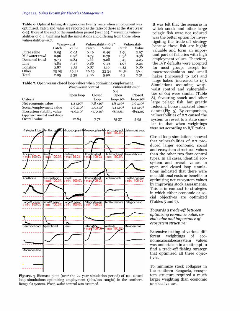
Page 122, Using Ecosim for Fisheries Management
It was felt that the scenario in which snoek and other large pelagic fish were not reduced was the better option for inves-tigating the trade-off strategy because these fish are highly valuable and form an impor-tant part of fisheries with high employment values. Therefore, the B/P defaults were accepted for most groups except for macrozooplankton and small hakes (increased to 1.0) and large hakes (increased to 1.5).
Simulations assuming wasp-waist control and vulnerabili-ties of 0.4 were similar (Table 8), favouring snoek and other large pelagic fish, but greatly reducing horse mackerel abun-dance (Fig. 5). By comparison, vulnerabilities of 0.7 caused the system to revert to a state simi-lar to that when weightings
were set according to B/P ratios. Closed loop simulations showed that vulnerabilities of 0.7 pro-duced larger economic, social and ecosystem structural values than the other two flow control types. In all cases, identical eco-system and overall values in open and closed loop simula-tions indicated that there were no additional costs or benefits to optimizing net ecosystem values by improving stock assessments. This is in contrast to strategies in which either economic or so-cial objectives are optimized (Tables 5 and 7). Towards a trade-off between optimizing economic value, so-cial value and importance of ecosystem structure: Extensive testing of various dif-ferent weightings of eco-nomic:social:ecosystem values was undertaken in an attempt to find a trade-off fishing strategy that optimized all three objec-tives. To minimize stock collapses in the southern Benguela, ecosys-tem structure required a much larger weighting than economic or social values.
Table 6. Optimal fishing strategies over twenty years when employment was optimized. Catch and value are reported as the ratio of those at the start (year 0-2): those at the end of the simulation period (year 22). * assuming vulner-abilities of 0.4, typifying half the simulations and differing from those when vulnerabilities=0.7.
Wasp-waist Vulnerability=0.4* Vulnerabil- Catch Value Catch Value Catch Value Purse seine 0.05 0.05 0.49 0.49 2.96 2.97Midwater trawl 0.96 0.96 0.79 0.79 0.38 0.38 Demersal trawl 3.73 2.84 5.66 3.28 5.45 4.25Line 3.84 3.47 0.86 0.19 1.07 0.24Longline 2.87 4.35 0.87 1.16 4.13 6.86 Other 25.05 29.41 26.59 33.34 28.38 36.4 Total 2.05 5.39 3.06 5.90 4.3 7.31
Table 7. Open versus closed loop values when optimizing employment.
Wasp-waist control Vulnerabilities of 0.4
Criteria
Open loop Closed loop
Open loopx105
Closed loopx103
Net economic value 1.3 x10⁶ 7.8 x10⁵ 1.8 x10⁵ 7.6 x10⁵ Social/employment value 2.6 x10⁵ 1.5 x10⁵ 3.1 x10⁵ 1.2 x10⁵ Ecosystem stability value (approach used at workshop)
-1.6x10³ -1.5x10³ -853.61 -893.05
Overall value 12.84 7.71 15.37 5.95
Figure. 3 Biomass plots (over the 22 year simulation period) of 100 closed loop simulations optimizing employment (jobs/ton caught) in the southern Benguela system. Wasp-waist control was assumed.

FAO/Fisheries Centre Workshop, Page 123
Even under a weighting of 1:1:10, and assuming the con-servative vulnerability setting of 0.4, chub mackerel, snoek, other large pelagic fish and hakes were eliminated from the system. Therefore a weighting of 1:1:25 for eco-nomic: social :ecosystem was adopted. Using the first method of evaluating ecosystem impor-tance, catch was increased by up to 50% and economic value between two and three-fold when ecosystem structure was optimized (Table 10). Catches, especially of cephalopods, were increased in the “other” gear fisheries and abundances of most groups increased or at least remained constant (Fig. 6). Two sets of optima were ob-tained using the second method to assess ecosystem structure (weighting accord-ing to B/Ps with increased values for macrozooplankton and hakes) and to find a trade-off between the three objectives. In the first, catches were doubled and economic values increased between five- and six-fold when wasp-waist control and vulnerabilities of 0.7 were as-sumed (Table 11). Similarly, in some simulations where vulnerabilities were propor-tional to trophic levels, and which began using random Fs, the same optimal strategy was found (Fig. 7). Such strategies caused col-lapses of chub mackerel, snoek and hakes by expan-sion of the demersal trawl fishery to four or five times its original size. These conse-quences differed from those under optimal trade-off fish-ing strategies obtained when vulnerabilities of 0.4 were as-sumed, and in some cases when vulnerabilities were proportional to trophic levels (Table 11).
Table 9 .Open versus closed loop values when optimizing ecosystem structure. Wasp-waist con-
trol Vulnerabilities of
0.4 Vulnerabilities of
0.7 Criteria
Open loop
Closed loop
Open loop
Closed loop
Open loop
Closed loop
Net econ. value 4.1 x10⁴ 3.0x10⁴ 3.7x10⁴ 2.8x10⁴ 4.8x10⁵ 2.9x10⁵ Social/employ. 8.3 x10³ 5.8x10³ 6.5x10³ 4.7x10³ 2.2x10⁴ 1.4x10⁴ Ecosystem stabil-ity (as at work-shop)
1.0x10³ 1.0x10³ 9.8x10² 9.8x10² 1.2x10³ 1.2x10³
Overall value 1.21 1.21 1.17 1.17 1.45 1.45
Table 8. Optimal fishing strategies over twenty years when optimal ecosystem structures were attempted using the revised (second) method. Catch and value are reported as the ratio of those at the start (year 0-2): those at the end of the simulation period (year 22).
Wasp-waist Vulnerability=0.4 Vulnerability=0.7 Catch Value Catch Value Catch Value Purse seine 0.10 0.10 0.08 0.08 0.12 0.12 Midwater trawl 0.17 0.17 0.32 0.32 2.03 2.03Demersal trawl 0.06 0.07 0.07 0.08 3.31 2.24Line 0.21 0.21 0.13 0.13 0.18 0.24 Longline 1.54 1.55 1.60 1.61 0.30 0.40 Other 0.72 0.63 0.47 0.41 0.76 0.73 Total 0.10 0.16 0.09 0.14 1.52 1.61
Figure 4 Biomass plots (over the 22 year simulation period) of 100 closed loop simulations optimizing ecosystem structure in the southern Benguela system when groups were weighted according to their B/P ratios. Wasp-waist control was assumed

Page 124, Using Ecosim for Fisheries Management
Under these conditions, catches were reduced to a third of original levels and economic values increased be-tween two- and threefold by large increases in the valuable longline and “other” fisheries and a reduction in the demer-sal fishery. The trade-off in the second set of strategies was a severe reduction in horse mackerel stock size (Fig 7).
In all cases using the second ecosystem approach, the purse seine fishery was closed, allowing anchovy and sardine stocks to grow, whereas under the first ecosystem method, a healthy purse seine fishery was maintained. However, both methods revealed a common goal of expanding the economic and socially valuable “other” gear fisheries, in particular to enhance catches of cephalopods. This
was achieved by increasing cephalopod biomass by a factor of between 15 and 36, in particular through a reduction in its predators (hakes and seals). There were no differences between open and closed loop simulation values when wasp-waist control was assumed (Table 12), suggesting little benefits in improving estimates of stocks and ef-fort regulation. Overall values for closed loop simulations were larger in the trade-off simulations than in those in which only one objective was opti-mized at a time (Table 12 cf. Tables 5,7 and 9). Vulnerability settings of 0.7 gave a net ecosystem stability value that was lower in open loop simulations than in closed loop simulations incorporating variability about stock assessments and methods of effort control. Assuming vulnerabilities of 0.7 may give rise to instabilities in the system and unrealistic optimal fishing strate-gies.
Table 10. Optimal fishing strategies over twenty years when optimal ecosystem structures were attempted using the first method (ecosystem importance) and weighting economic:social:ecosystem importance as 1:1:25. Catch and value are reported as the ratio of those at the start (year 0-2): those at the end of the simulation period (year 22).
Wasp-waist Vulnerability=0.4 Vulnerability=0.7 Catch Value Catch Value Catch ValuePurse seine 0.99 0.99 0.23 0.23 1.47 1.47 Midwater trawl 3.07 3.07 1.53 1.53 0.33 0.33 Demersal trawl 1.13 1.16 1.63 1.5 1.12 1.17Line 0.97 0.91 0.62 0.57 0.44 0.37Longline 1.37 1.38 1.89 1.91 1.58 1.59Other 16.79 17.23 16.77 18.61 16.53 18.18 Total 1.27 2.88 1.07 3.12 1.49 3.01
Table 11. Optimal fishing strategies over twenty years when a trade-off between economic value, employment value and ecosystem structure was achieved by relative weighting of these three objectives: 1:1:25 using the revised method of ecosystem weighting. Catch and value are reported as the ratio of those at the start (year 0-2): those at the end of the simulation period (year 22).
Wasp-waist Vuln.=0.4 Vuln.=0.7 Vuln. α TL Catch Value Catch Value Catch Value Catch Value Purse seine 0.00 0.00 0.00 0.00 0.00 0.00 0.01 0.01 Midwater trawl
0.21 0.21 0.28 0.28 0.23 0.23 0.02 0.02
Demersal trawl
3.75 2.93 0.01 0.01 4.65 3.95 0.01 0.01
Line 0.23 0.28 0.03 0.03 0.10 0.12 0.03 0.03 Longline 0.75 1.11 30.43 30.78 0.34 0.57 27.78 28.15 Other 25.31 28.12 19.16 18.16 28.59 33.59 21.05 20.66 Total 1.95 5.03 0.36 2.42 2.37 6.28 0.38 2.65
Figure. 5 Biomass plots (over the 22 year simulation period) of 100 closed loop simulations optimizing ecosystem structure in the southern Benguela system when groups were weighted according to their B/P ratios, with the exceptions of macrozooplankton and small hakes (set to 1) and large hakes (set to 1.5). Wasp-waist control was assumed.

FAO/Fisheries Centre Workshop, Page 125
Conclusions (i) Fishing strategies that optimize economic value or employment are understandable and can be explained. (ii) These simulations often give rise to extreme alternative fishing policies and highlight the im-portance of carefully defining the objectives for setting a new fishing strategy in a particular sys-tem. (iii) The way in which a system is pre-sumed to function (vulnerability set-tings) can have major implications for the choice of optimal fishing strategy under certain objectives. (iv) In contrast to optimizing economic or social values, there is not as much clarity in how to optimize ecosystem stability or structure. This is partly be-cause the latter includes some subjec-tivity in the selection of groups to be given higher weightings, or even to be “monitored” when testing for reason-able optimal strategies. (v) The trade-off fishing strategy se-lected depends on how much relative weighting is given to each objective i.e. it is somewhat subjective and depends on the importance given to a stable ecosystem structure. (vi) The 1:1:25 economic: social: eco-system weighting using the first method to find a trade-off strategy was similar to that using the second ecosys-tem optimization method in that both
optimized cephalopod catches. This provides con-fidence in the overall conclusions drawn about theoretical optimization of fishing strategies in the southern Benguela system given specific theo-retical objectives. (vii) When ecosystem structural weightings were considered to be proportional to trophic levels, the optimal trade-off fishing strategy was consis-tent with those obtained when wasp-waist control and vulnerabilities of 0.4 were assumed. There-fore this general guideline to setting of vulner-abilities is promising. (viii) The larger variability between the 100 means of closed loop simulations when vulner-abilities were 0.7 than when wasp-waist control or 0.4 vulnerabilities were assumed, suggests that smaller vulnerabilities are probably preferred for the southern Benguela upwelling system. Wasp-waist flow (bottom-up control of predators by small pelagic fish and top-down control of zoo-plankton by small pelagic fish) gave reasonable results.
Optimiz ing the ecosystem objective:
method one
05
101520
mac
rozo
opla
nkto
n sard
ine
hors
em
acke
rel
ceph
alop
ods
othe
r de
mer
sal
fish
seab
irds
End/
star
t wasp-waist
v=0.4
v=0.7
Figure. 6 Comparing end/start biomasses of major groups in the southern Benguela system under three vulnerability settings, when the first method of opti-mizing ecosystem importance was used to find a trade-off between economic, social and ecosystem objectives by relative weightings 1:1:25.
Fig. 7 Biomass plots (over the 22 year simulation period) of 100 closed loop simulations finding an optimal trade-off between economic, social and ecosystem objectives (weighted 1:1:25) in the southern Benguela system when the revised ecosystem weighting method was used and vulnerabilities were proportional to trophic levels.

Page 126, Using Ecosim for Fisheries Management
References Cochrane, K.L. and A.I.L.Payne 1998. People, Purses
and Power: Developing fisheries policy for the new South Africa. Pages 57-71 in T.J.Pitcher, P.J.B.Hart and D.Pauly (eds) Reinventing Fisheries Manage-ment. Kluwer Academic, Dordrecht, Netherlands. 435 pp.
Cury, P., Bakun, A., Crawford, R.J.M., Jarre-Teichmann, A., Quinones, R.A., Shannon, L.J. and Verheye, H.M. 2000. Small pelagics in upwelling systems: patterns of interaction and structural changes in “wasp-waist” ecosystems. Academic Press, ICES Journal of Marine Science, Sympo-sium Edition 57(3): 603-618.
Jarre-Teichmann, A., Shannon, L.J., Moloney, C.L. and Wickens, P.A. 1998. Comparing trophic flows in the southern Benguela to those in other upwelling ecosystems. In Pillar, S.C., Moloney, C.L., Payne, A.I.L. and Shillington, F.A. Benguela dynamics: impacts of variability on shelf-sea environments and their living resources. S. Afr. J. mar. Sci. 19: 391-414.
Shannon, L.J., Cury, P and Jarre, A. 1999. Modelling effects of fishing in the southern Benguela ecosys-tem. Academic Press. ICES Journal of Marine Sci-ence, Symposium Edition 57(3):720-722.
Shannon, L.J. in prep. Modelling trophic flows through the southern Benguela upwelling system, towards provision of ecosystem management advice. Ph.D. thesis to be submitted - end 2000.
Stuttaford, M. (ed.) 2000. Fishing Industry Handbook: South Africa, Namibia and Moçambique. Exbury Publications, Cape Town, South Africa. 404 pp.
Table 12. Open versus closed loop values for a trade-off between economic value, social value and ecosystem structure using the revised method of ecosystem weighting. * = approach used at workshop.
Wasp-waist control Vuln.= 0.4 Vuln.= 0.7 Vuln. α TL Criteria Open
loop Closed
loop Open loop
Closed loop
Open loop
Closed loop
Open loop
Closed loop
Net economic value 1.3 x10⁶ 1.3x10⁶ 4.6x10⁵ 3.1X10⁵ 1.6x10⁶ 7.3x10⁵ 4.9x10⁵ 3.3x10⁵ Social value 2.3x10⁵ 2.3x10⁵ 1.6x10⁵ 1.1X10⁵ 2.8x10⁵ 1.4x10⁵ 1.8x10⁵ 1.1x10⁵ Ecosyst. stability* 1.1x10³ 1.1x10³ 9.2x10² 9.2X10² 1.1x10³ 1.2x10³ 9.3x10² 9.3x10² Overall value 50.79 50.79 38.38 34.76 56.08 45.66 39.37 35.37

FAO/Fisheries Centre Workshop, Page 127
Impact of harvesting strategies on fisheries and community structure on the Continental Shelf of the Campeche Sound, Southern Gulf of Mexico Francisco Arreguin-Sanchez CICIMAR, La Paz, Baja California Sur, Mexico Abstract An analysis of harvest strategies for the ecosystem of the Campeche Sound, Southern Gulf of Mexico, was conducted based on a mass-balance model previously published, and making some emphasis on the shrimp fishery, which is strongly depleted. In the ecosystem model four fleets were identified, the shrimp and three artisanal fleets associated with the fishing gear and tar-get species. A time series of estimated biomass (and corrected because of a depensatory effect) and fishing pattern for the shrimp fishery, for the period of 1974 to 1993 was contrasted with Ecosim shrimp-biomass simulation, also involving forcing factors representing one of the main causes for shrimp-biomass depletion. Besides this simulation, seven harvesting strategies were simulated by optimizing different criteria such as economic rent, social (employment) and ecosystem stability, as well as a combination between them. The impact of different strategies on biomass groups, on the uncertainty, and how biomass changes with trophic level was measured. Changes in vulnerability to preda-tion and in the mean trophic level were also explored. Simulations were conducted under different harvesting strategies considering optimization of economic rent, jobs and ecosystem stability criteria combined, as well as the ecosystem stability criterion alone. During such simulations some conditions were modified such as the weighting factors on ecosystem criteria and uncertainty per group; weighting factors for the impact of fleets, and annual changes in catchability per fleet. Simulated biomasses were compared with some fixed levels of biomass as reference points. In general terms most scenarios caused a depletion of some groups below the critical level of 50% of the starting biomass, which was here considered as an undesirable level. Even more sharks tend to disappear during the first years of simu-lation. A scenario where the ecosystem structure crite-rion was optimized, shows no depletion of any group. For all the cases, shrimp showed an uncertain behavior during the terminal years of the simulation, always as-sociated with the effect of forcing factors. However, for the scenario optimizing an ecosystem structure crite-rion, shrimp uncertainty was lower.
Introduction The continental shelf of the Campeche Sound on the Southern Gulf of Mexico is a complex ecosys-tem accounting for the use and exploitation of the natural resources. In this area the oil industry ex-
tracts around 70% of the oil and natural gas pro-duced in the country, and converges with other activities, mainly fisheries and services (mainly transport). The Campeche Sound has historically been im-portant because of the exploitation of shrimp re-sources. Before the oil industry was established (early 80's), fishing, and particularly the shrimp fishery, was the center of the regional economy. Landing records show that for many years shrimp was practically the only species exploited; other species did not appear in the statistics. Higher yields were obtained during early 1970’s with around 27,000t per year, of which 90% was the pink shrimp (Farfantepenaeus duorarum). Cur-rently this fishery is collapsed, with yields close to 3,000t per year. The main problem with this fish-ery is that recruitment rate has continuously de-clined since the 1970’s, and is highly influenced by environmental factors such as salinity, which has decreased markedly since the mid-80’s. In-creasing sea surface temperature has reduced stock abundance. In both cases, correlation analysis indicates values above r2=0.7 (Ramírez-Rodríguez et al. 2000). With decrease in the shrimp stock, there has been more targeting of other fish. The ecosystem approach to explore the impact of harvest strategies is based on a model constructed with Ecopath with Ecosim software (Christensen and Pauly 1992, Walters et al. 1997) by Manik-chand-Haileman et al. (1998), and it is based on information on biomass taken from surveys dur-ing the period August 1988 to July 1994. The eco-system comprises an area of 65,000km2, where the shrimp fishery commonly operates with a cur-rent fleet size of around 320 boats. In this area, close to the coast, some artisanal fisheries also operate. Recent statistics indicate the existence of more than 4400 boats in the artisanal fleet. De-tails of the basic data, related to the construction of the model and ecosystem statistics, can be con-sulted in Manikchand-Haileman et al. (1998), while main biomass flows are shown in Figure 1.
Table 1. List of strategies.
Strategy Description Strategy 1 Leave things under the current tendency.
This is taken as the base scenario Strategy 2 Optimize economic benefits over social and
ecological benefits Strategy 3 Optimize social benefits in terms of jobs Strategy 4 Optimize ecosystem benefits in terms of
ecological quality/conservation Strategy 5 Optimize economic, social and ecological
benefits as an ideal scenario Strategy 6 Optimize economic and social benefits Strategy 7 Optimize social and ecological benefits Strategy 8 Optimize economic and ecological benefits

Page 128, Using Ecosim for Fisheries Management
In 2000, the National Institute of Fisheries in Mexico met a panel of experts to analyze the situation of the shrimp fishery in the Campeche Sound. The main conclusions were classified un-der three major issues: the impact of the fishery (overcapitalization, overfishing), the quality of the environment (which in some areas has been al-tered by natural and human-induced causes), and social aspects (loss of employment and inability to control illegal fishing). The aim of this contri-bution is to test harvesting strategies of the fish-eries of Campeche Sound in the context of the ecosystem, and to evaluate the impact of potential management policies. Material and Methods The previously published model contains 11 groups: fishes, sharks, shrimp, squids, epifauna, infauna, zooplankton, phytoplankton and detri-tus. There are two types of fisheries, shrimp trawling and artisanal fisheries. The latter was di-
vided in three groups by target species and fishing gear. The artisanal-demersal fleet mostly uses short longlines and hand-based hooks; this fleet target on groupers, snappers among others. The artisanal-pelagic fleet mostly uses gillnets to catch mackerels, jacks, and hook-lines for sharks; and the beach seine fishery, which operates in some localities exploiting a number of species. Harvesting strategies were tested for the optimi-zation of three major criteria, economic benefits in terms of net profits, social benefits in terms of employment (social benefits) generated by the fisheries, and ecosystem benefits in terms of maintenance of the stocks (ecosystem stability). Under this context eight strategies were tested as in Table 1. Preparing the base scenario (Strategy 1) Catch values were obtained from statistical re-cords reported by the ministry of fisheries (SEMARNAP, 1998) as landed prices. Costs were represented as proportions as in Table 2. Time series were used to calibrate simulated bio-masses. In this case, the available data corre-sponded to harvest rates and estimated biomasses for the shrimp fishery which were previously es-timated through a non-equilibrium biomass dy-namic model (Schaefer 1957, Hilborn and Walters 1992) and corrected by non-compensatory effects
Table 2. Costs per fleet. Fleet
Fixed cost
(%)
Effort related
cost (%)
Sailing related
cost (%)
Profit
(%)
Shrimp 5 40 10 55Art DEM HL 2 20 1 77 Art PEL 2 30 3 65 Art Beach Seine 2 10 0 88
Figure. 1 Biomass-flow diagram for the ecosystem of the continental shelf of the Campeche Sound, Mexico. Biomass (B), Consumption (Q) and fishery harvest are in g m-2 wet weight; all flows are in g m-2 year-1 (taken from Manikchand-Haileman et al. 1998).

FAO/Fisheries Centre Workshop, Page 129
(unpublished data1). Time se-ries cover the period of 1974 to 1994. A significant correlation with forcing factors and shrimp abundance were found, particu-larly sea surface temperature and salinity, being the last an inverse relationship. Here salin-ity was incorporated as forcing factor affecting shrimp group. Vulnerabilities to predation were assumed to be v = 0.3, representing mixed control of flows of biomass by predators and preys. For all strategies the mean tro-phic level of the ecosystem, MTLE, was computed based on simulated biomasses:
∑∑==
=n
1ii
n
1iii BTLBMTLE
where Bi = biomass of the stock i, and TLi = the mean trophic level of the stock i. Testing Strategies Applying specific objective functions, all the strategies were tested; for this, a very low weight was assigned to the undesirable criteria, and unit weight to the objective criteria. A null ecological weight (zero) was assigned to each group, with exception of shrimp, where the weight was unity. For the social criteria, defined as the Job/Catch ratio, the assigned values for each fishery were as follows: shrimp=0.5, art-DEM HL=1.7, art-PEL=1.7 and art-beach seine=2.0. In a trophic model, vulnerability to predation can be an important factor defining simulated bio-mass trajectories. Arreguín-Sánchez (2000) showd that modelled octopus biomass is unstable with low values of vulnerability to red grouper on the continental shelf of Yucatan. The same occurs under high vulnerabilities combined with high fishing pressure. In the present case, the explora-tion of the vulnerability parameter is useful be-cause of the stress to which shrimp stock is cur-rently subjected. In addiotion to the EwE default value (v = 0.3), three scenarios were tested with values v = 0.2, v = 0.4 and v = 0.7, where lower
1 A. Navarrete del Proó and F. Arreguín-Sánchez. 2000. Deple-tion of the pink shrimp fishery on the Campeche Bank. INP-Campeche, CICIMAR-IPN. Mexico. 17p.
and higher values represent bottom-up and top-down control, respectively. Another aspect to be considered is the starting fishing rate, F, to be used for simulations. In this case two scenarios were tested, selecting current F’s as starting state, or selecting random F’s val-ues. The difference is that during simulations fishing rate can follow a different routes to arrive at the optimization for a particular objective func-tion. Closed loop simulation The performance of the simulations above can be improved by specifying some factors affecting the fishery. Here the incorporation of uncertainty for risk analysis, changes in catchability with time, the relative impact of the fishery and the com-parison with some biological reference points were considered. All strategies were tested under this scope, and for particular situations, with em-phasis on the shrimp stock. Results Strategy 1, as the base scenario, leaves things running under the current pattern, also repre-senting the state of the ecosystem against which others strategies can be compared. Time series and a forcing factor (salinity anomaly) were in-corporated as mentioned above.
Figure 2. Ecosim simulated biomass (line) contrasted with independ-ent estimates of biomass (dots) and real fishing pattern (black bars on the bottom) for the pink shrimp (F. duorarum) on the Campeche Sound, Mexico, for the period 1974 to 1993. Diagram on the top-right side shows the anomaly of salinity used as forcing factor.

Page 130, Using Ecosim for Fisheries Management
Figure 2 shows simulations performed which, for the case of shrimp, exhibit an unstable behavior at the end of the period. This unstable behavior is a consequence of environmental effects plus the fishing stress imposed by the fishery. Ramírez-Rodríguez et al. (2000a, b) explain this in terms of the impact of the forcing factors on recruitment patterns and reproduction success. In terms of the model, simulations appears to fit independent data reasonably well. Comparing Strategies Table 1 summarizes outputs of different strategies with respect to their impact on biomasses. In general terms the most important stocks, from the fishing point of view, shrimp, groupers and snappers were always posi-tively impacted for all strategies, or at least not strongly afected in a negative sense. Except for Strategy 4 (optimizing ecological benefits), all strategies imply negative effects on at least one stock, tak-ing as a criterion reduction of biomass be-low 20% of that of the base scenario. Strategy 5, optimizing three criteria simul-taneously, represents the next best strat-egy in terms of biomass. Seven stocks in-crease in biomass while two decrease, but one of them disappears (sharks). Strate-
gies 6, 7 and 8 (optimizing two criteria) show 4 stocks increased and seven decreased, with one of them disappearing (sharks). As expected, biomasses decrease with trophic level for all strategies, at a rate of around 12% (Fig. 3a), corresponding roughly to the transfer efficency suggested by Pauly and Christensen (1995); but also refecting harvesting strategies. Coefficients of variation of biomass for the differ-ent strategies tend to increase with TL, with the exception of strategy 3 (maximize jobs), which decreases with trophic level. This behavior is likely due to the construction of the social index (Job/Catch), and suggests lower uncertainty in
Table 1. Simulated average biomass (top) and its coefficient of variation (bottom) for commercial groups on the Campeche Sound, Southern Gulf of Mexico, for different harvesting strategies (S#). $, J and E indicate optimization for economic, job and ecosystrem criteria. Biomasses decreasing below 20% of starting biomass are between brackets. Bold numbers indicate higher values of biomass with respect to the starting value (For explanation see text).
Average biomass Her Jac Mac Fla Cat Moj Sna Cro Gro Gru Sha O_f Squ Shr
S1 (=base) 6.18 1.84 1.08 0.91 0.70 0.85 0.11 0.46 0.47 0.23 0.09 0.53 0.11 1.41
S2 (=M$) 3.18 1.69 0.36 1.51 (0.04) (0.04) 0.13 (0.10) 0.72 (0.10) 0.12 0.22 0.04 1.91
S3 (=MJ) 5.65 (0.10) (0.02) 1.66 (0.04) (0.04) 0.12 (0.10) 0.51 (0.10) (0.00) 0.40 0.12 2.05
S4 (=ME) 6.57 1.84 1.17 0.85 0.80 0.93 0.10 0.48 0.46 0.24 0.09 0.54 0.12 1.00
S5 (=M$JE) 6.47 1.75 0.56 1.20 0.27 0.40 0.11 0.10 0.48 (0.05) (0.00) 0.56 0.14 1.74
S6 (=M$J) (0.24) (0.31) (0.02) 2.23 (0.03) (0.02) 0.12 (0.10) 0.62 (0.10) (0.00) 0.19 0.07 2.45
S7 (=MJE) 5.70 (0.10) (0.02) 1.66 (0.04) (0.04) 0.08 (0.10) 0.49 (0.10) (0.00) 0.30 0.08 0.90
S8 (=M$E) (0.25) 0.47 (0.03) 2.18 (0.03) (0.02) 0.12 (0.10) 0.64 (0.10) (0.00) 0.19 0.06 2.35
Coefficient of variation
Her Jac Mac Fla Cat Moj Sna Cro Gro Gru Sha O_f Squ Shr
S1 (=base) 16.92 8.63 17.61 2.62 15.37 16.05 24.05 23.40 15.29 23.14 22.43 9.00 13.68 29.22
S2 (=M$) 18.37 6.94 38.20 17.79 (263.6) (287.54) 32.85 (362.28) 22.34 (310.77) 14.34 37.51 51.13 26.57
S3 (=MJ) 5.65 (0.10) (0.02) 1.66 (0.04) (0.04) 0.12 (0.01) 0.51 (0.01) (0.00) 0.40 0.12 2.05
S4 (=ME) 2.50 2.46 1.80 4.43 4.17 2.28 23.31 11.93 14.83 14.84 5.42 3.95 6.10 52.15
S5 (=M$JE) 5.12 2.81 14.91 9.26 52.66 28.26 25.73 88.80 14.45 (93.26) (319.72) 7.63 12.30 25.06
S6 (=M$J) (256.76) (111.83) (479.16) 28.57 (361.14) (432.93) 30.58 (510.11) 22.58 (433.27) (770.08) 40.10 51.91 31.43
S7 (=MJE) 12.10 (284.0) (630.10) 21.31 (281.73) (323.14) 20.16 (416.22) 16.06 (353.73) (871.72) 11.50 14.29 68.97
S8 (=M$E) (249.05) 71.57 (439.75) 28.17 (356.98) (426.51) 30.24 (503.85) 23.01 (428.12) (701.42) 42.76 53.03 32.23
Her = Herrings, Jac = Jacks, Mac = Mackerels, Fla = Flatfish, Cat = Catfish, Moj = Mojarra, Sna = Snappers, Cro = Croakers, Gro = Groupers, Gru = Grunts, Sha = Sharks, O_f = Other fish, Squ = Squids, and Shr = Shrimps.
Table 2 Mean trophic level of the ecosystem computed for simu-lated harvesting strategies and changes in vulnerability (Vul) to predation. Low value between brackets; higher value in bold. $, J and E represent economic, job and ecosystem stability criteria. S#’s represent strategies (for explanation see text)
Control Type Vul = 0.2 Vul = 0.3 Vul = 0.4 Vul = 0.7 Strategies (bottom-up) (mixed) (mixed) (top-down)
S1 (=base) - 2.330 - -S2 (=M$) (2.200) 2.282 2.345 2.446 S3 (=MJ) 2.204 2.274 2.309 2.461 S4 (=ME) 2.326 2.336 2.330 2.325 S5 (=M$JE) 2.215 2.319 2.346 2.349 S6 (=M$J) - 2.228 - - S7 (=MJE) - 2.268 - - S8 (=M$E) - 2.229 - -

FAO/Fisheries Centre Workshop, Page 131
employment if fisheries target high trophic levels (Fig. 3b). With respect to the fleets, the ratio between the last year of simulation to the starting year was used to evaluate the relative effect of the harvest strategies. The only fleet which improves biomass under all strategies was the artisanal fishery tar-geting demersal fishes (art-DEM HL), which captures mostly high-priced species. The strategy which shows the best overall condition for all fleets was that which optimizes economic criteria (Strategy 2), but it is not a clear improvement on the base scenario. Changes in vulnerability to predation suggest that mixed control involves less uncertainty in biomasses (ex-pressed by the coefficient of varia-tion) than ‘bottom-up’ or ‘top-down’ controls. For bottom-up control (V=0.2), higher uncertainty was ob-served for intermediate trophic lev-els. For top-down control (V=0.7), higher uncertainty was associated with higher trophic levels. However, a relatively constant, low uncertainty was observed for mixed control (Fig. 4). These aspects should be given fur-ther investigation because ecosystem mechanisms behind the observed behaviour could explain what hap-pens in those cases where top preda-tors have been removed from the ecosystem.
Mean trophic level of the ecosystem (MTLE) was computed for a different combination of strate-gies and vulnerabilities (Table 2). Strategies, which optimize economic yield and jobs show a proportional increase of MTLE with vulnerability. A strategy optimizing the three criteria shows a decrease in MTLE with low vulnerability (v = 0.2) corresponding to ‘bottom-up control’, but no
A B
0.01
0.10
1.00
10.00
100.00
0 1 2 3 4 5
Trophic level
Log
Bio
mas
s
0.1
1
10
100
1000
0 1 2 3 4 5Trophic level
Log
CV B
0.0001
0.01
1
100
0 1 2 3 4 5
Trophic Level
Log
CV B
JOBS
Figure 3. Changes in biomass (A) and the corresponding coefficient of variation (B) with trophic level for different harvesting strategies simulated with Ecosim. White dots are for strategy 1 (base scenario). Note the inverse relation-ship when jobs are optimazed (for explanation see text).
Figure. 4. Effect of changes in vulnerability in Strategy 2 (optimizing the economic criterion). A) on group biomasses, and B) on uncertainty of biomass by trophic level. Low values for vulnerability, v=0.2 (dashed line and black squares) indicate bottom-up control; high values, v=0.7 (thin line and white circles) top-down and intermediate values mixed control, v=0.4 (bold line and white squares).
0.00
0.00
0.01
0.10
1.00
10.00
100.00
1 2 3 4 5 6 7 8 9 10 11 12 13 14 15 16 17 18 19
Functional groupLog
biom
ass
A
0
250
500
750
1000
0 1 2 3 4 5
Trophic Level
CV B
B

Page 132, Using Ecosim for Fisheries Management
change was produced for mixed and ‘top-down control’ (v ≥ 0.3). Strategy 4, optimizing ecosys-tem stability, did not change with vulnerability (Fig. 5). Starting simulations with current F’s vs. Random F’s The reason for this test was to observe the effect of running a given strategy by using a predefined F (i.e. current fishing mortality) to initiate simu-lations. The use of random values of F will gener-ate a number of iterations, which could change the way in which a simulation approaches the so-lution of the objective function. In all the cases, the results at the end of the simulation were the same. Further work on simulations will initiated by using random F. Closed loop simulations For this analysis, uncertainty was incorpo-rated through the coefficient of variation as-sociated with each group. The fleet impact on the ecosystem was also provided by a weighting factor, in this case I assumed that the artisanal fleet do not cause an impact (factor = 1X), while the shrimp fleet factor was 3X. Changes in catchability with time were also considered in different ways. The upper and lower bounds in biomass of the groups were used as biological reference points to evaluate the state of the stock. Conditions for simulations are defined in Table 3. For all the strategies, the shrimp stock be-comes unstable in the last years of simula-
tion, but this behaviour is associated with forcing factors as mentioned previously. For the two sce-narios related to Strategy 5, croakers and grunts fall below the level of 0.5B at the end of the simu-lated period; while sharks fall below this level, disappearing before year 10 of the simulation (Figure 6). For Strategy 4, and with the exception of shrimp, there no stocks declined below the ref-erence point of 0.5B (Fig. 7). Performance index The weighted total objective performance was computed for each scenario mentioned above, and same selected outputs are shown in Table 4. Discussion
Table 3. Conditions established for harvesting scenarios during close loop simulations.
CV RIF max ∆q wfS Strategy 4, optimizing economic rent, jobs and ecosystem stability
Scenario 1 0.2 all (groups) 1 all 0.1 all 1 Scenario 2 0.2 all 3 Shrimp, 1 others 0.2 Shrimp, 0.05 others 1 Scenario 3 0.2 all 1 all 0.1 all 5 Scenario 4 0.2 all 3 Shrimp, 1 others 0.2 Shrimp, 0.05 others 5 Scenario 10 0.4 Shrimp, 0.2 all 3 Shrimp, 1 others 0.2 Shrimp, 0.05 others 1 Scenario 11 0.4 Shrimp, 0.2 all 3 Shrimp, 1 others 0.2 Shrimp, 0.05 others 5
Strategy 3, optimizing ecosystem stabilityScenario 5 0.2 all 1 all 0.1 all 1 Scenario 6 0.2 all 3 Shrimp, 1 others 0.2 Shrimp, 0.05 others 1 Scenario 7 0.2 all 1 all 0.1 all 5 Scenario 8 0.2 all 3 Shrimp, 1 others 0.2 Shrimp, 0.05 others 5 Scenario 9 0.4 Shrimp, 0.2 all 3 Shrimp, 1 others 0.2 Shrimp, 0.05 others 5 CV = coefficient of variation, RIF = relative impact of the fishery, max ∆q = maximum rate of catchability increase. WfS = ecologi-cal weighting factor assigned to Shrimp group at the beginning of simulations.
2.15
2.20
2.25
2.30
2.35
2.40
2.45
2.50
0 0.2 0.4 0.6 0.8
vulnerability
MTL
E
Figure. 5 Changes in the mean trophic level for the ecosystem (MTLE) as a function of vulnerability. Strategy maximizing eco-system stability is not affected (bold line); Strategies maximizing economic rent and jobs increase in proportion to vulnerabil-ity(dashed and dotted lines, respectively). Strategy optimizing the three criteria (thin line) increases for transition between bot-tom-up to mixed control, and remains stable from mixed to top-down control.

FAO/Fisheries Centre Workshop, Page 133
Currently, Ecopath with Ecosim constitutes a useful tool to explore harvesting strategies. The incorporation of independent estimations of biomass and fishing patterns provides an important possibility for its use for exploring management strategies. Moreover, the application of objective functions to optimize single or multiple criteria, the impact of fleets, changes in catchability with time as well as uncertainty, give a good opportunity to consider an ecosystem framework for management purposes. Simulated strategies give a number of scenar-ios concerning changes in ecosystem pools, which change in different ways. Strategy 4 (optimizing ecosystem stability) was the only option which did not provoke decline in the biomass of any group; moreover, biomass in-creased in most of them. Moreover, the most important resources, shrimp, groupers and snappers were reduced under any strategy tested. However, groups like grunts, croakers, mojarra, catfish and sharks were reduced un-der most strategies, as measured by a decline in biomass below 20% of base scenario (Strategy 1). Sharks disappeared in most cases. It was also noticed that when a simula-tion optimized only two criteria, several groups were reduced, but with high uncer-tainty, as expressed by the coefficient of varia-tion (Table 1). Decrease of biomass with trophic level (Fig. 3a) for all strategies appears to be associated with transfer efficiencies. However, those data also reflect fishing stress imposed by exploi-tation, suggesting that the rate of change could be lower for unexploited systems. This could be an impact on biodiversity. In this sense, more inves-tigation is required. Vulnerability to predation, related to the type of biomass-flows control, suggests that, for mixed
control, uncertainty decreases, while the opposite applies to top-down or bottom-up control. This uncertainty also suggests that a more stable sys-tem might obtain under mixed control. This is a research line to be explored, because it could be associated with removal large predators in an ecosystem, such as has occurred in some
collapsed fisheries. Ar present, the problem of the pink shrimp (F. duorarum) fishery in Campeche Sound is a great challenge for scien-tists, managers and fish-ers in Mexico. The main question here is, what can we do to rebuild this fishery? Initially the role of the forcing factors is ex-tremely important creat-
Table 4. Weighted total performance indices for simulation of harvesting strategies.
Criteria
Strategy 5 max ($JE) Scenario 4
Strategy 4 max (ME) Scenario 9
Strategy 5 max ($JE) Scenario 11
Open Loop
Closed Loop
Open Loop
Closed Loop
Open Loop
Closed Loop
Net Economic Value 3012.81 2486.52 420.17 1733.4 3012.95 2531.03 Social value (employ.) 2887.83 2047.38 1645.64 1586.6 2887.84 2069.5 Ecosystem stability -44.46 -43.61 -23.1 -21.06 -44.46 -43.97 Overall value 0.66 0.4 -0.23 -0.21 0.66 0.41
Relative index (Close Loop / Open Loop) Net Economic Value 0.825 4.125 0.840 Social (employ.) value 0.709 0.964 0.717 Ecosystem stability 0.981 0.912 0.989 Overall value 0.606 0.913 0.621 Figure 6 7
Figure 6. Simulated biomasses from close loop simulation for Strategy 4 (optimizing economic, jobs and ecosystem crite-ria) under the following conditions: a) assigning a factor of 1 to ecosystem criteria as well as for the shrimp group. b) As-signing uncertainty to biomass for each group as CV = 20%. c) Shrimp fleet impact ecosystem three times respect to the ar-tisanal fleets. d) Catchability for artisanal fleets increases 5% each year while for shrimp fleet 20%. e) Reference biological level of biomass (dashed lines) fixed at 0.5B and 2.0B. Note that Croakers, Grunts and Sharks fall below critical level of 0.5B, and Shrimps maintain large uncertainty during the last period because the effect of forcing factors.

Page 134, Using Ecosim for Fisheries Management
ing both low stock abundance and uncer-tain biomass and fishery behavior (Figure 2) at the end of the period. During The simulations measured social impact as the Job/Catch ratio. In the shrimp fishery, employment is now around 10% of that in the mid-1970’s, while yields have col-lapsed. Evidently, some fishers have con-tinued fishing despite low yields, a chnge that can modify the Job/Catch ratio. Some looked for alternative fishing jobs, adding fishing pressure to alternative fish re-sources. Some other fishers migrated to other sectors. These social dynamics are not captured by the fixed values in the simulation model. In general terms, best option from the si-mautions is Strategy 4 (Fig. 7), which op-timizes the ecosystem stability criteria. Other options tested, such as optimizing economic, social and ecological criteria simultaneously, yield some undesirable scenarios, since some stocks decline and sharks tend to disappear. Acknowledgments I would like to acknowledge to Dr. Kevern Cochran from FAO for his invitation to partici-pate in the FAO / UBC Fisheries Centre work-shop on “The use of ecosystem models to in-vestigate multispecies management strategies for capture fisheries”. Thanks also to the Japan Government who financed me for this activity, and to the National Polytechnic Institute, Mex-ico, for partial support through CEGEPI-980056 project, COFAA and EDI. References Arreguín-Sánchez, F. 2000. Octopus-red grouper in-
teraction in the exploited ecosystem of the north-ern continental shelf of Yucatan, Mexico. Ecologi-cal Modelling (in press).
Christensen, V. and D. Pauly. 1992. Ecopath II- a soft-ware for balancing steady – state ecosystem mod-els and calculating network characteristics. Eco-logical Modelling 61: 169-185
Hilborn, R. and C. J. Walters. 1992. Quantitative fisher-ies stock assessment. Chapman and Hall. New York, 570pp.
Manikchand-Haileman, S., L.A. Soto and E. Escobar. 1998. A preliminary trophic model of the continen-tal shelf, South-western Gulf of Mexico. Estuarine, coastal and shelf Science. 46: 885-899
Pauly, D. and V. Christensen. 1995. Primary production required to sustain global fisheries. Nature 373: 255-257
Ramírez-Rodríguez, F. Arreguín-Sánchez and D. Lluch-Belda. 2000a. Collapse of the pink shrimp Far-fantepenaeus duorarum(Burkenroad, 1939) fishery and sea surface temperature in Southern Gulf of Mexico. (submitted to Fish. Bull.)
Ramírez-Rodríguez, M. E.A. Chávez and F. Arreguín-Sánchez. 2000b. Perspective of the pink shrimp (Farfantepenaeus duorarum Burkenroad) fishery of the Campeche Bank, Mexico. Ciencias Marinas, 26(1):97-112
Schaefer, M. B. 1957. A study on the dynamics of the fishery for yellowfin tuna in the eastern tropical Pacific Ocean. Inter-Am. Trop. Tuna Comm. Bull. 2:247-285
SEMARNAP. 1998. Anuario estadístico de pesca 1997. Secretaría de Medio Ambiente, Recursos Naturales y Pesca. México. 241pp.
Walters, C., V. Christensen and D. Pauly. 1997. Struc-turing dynamic models of exploited ecosystems from trophic mass-balance assessments. Reviews in Fish Biology and Fisheries. 7: 1-34
Figure. 7 Simulated biomasses from close loop simulation for Strategy 3 (optimizing ecosystem criteria) under the following conditions: a) assigning a factor of 5 to ecosystem criteria as well as for the shrimp group. b) Assigning uncertainty to biomass for each group as CV = 20%, except for shrimp with CV = 40%. c) Shrimp fleet impact ecosystem three times respect to the artisanal fleets. d) Catchability for artisanal fleets increases 5% each year while for shrimp fleet 20%. e) Reference biological level of bio-mass (dashed lines) fixed at 0.5B and 2.0B. Note that Croakers, Grunts and Sharks remains at "health" levels of biomass (>0.5B), and Shrimps maintain uncertainty during the last period because the effect of forcing factors.

FAO/Fisheries Centre Workshop, Page 135
Evaluating harvesting strategies for fisheries in the Central Gulf of California ecosystem Francisco Arreguín-Sánchez1 and Luis E. Calderón-Aguilera2
1CICIMAR, La Paz, Mexico 2CICESE, Ensenada, Mexico Abstract Harvesting strategies were tested for fisheries of the west-central region of the Gulf of California. Simula-tions using Ecosim were based on a previously con-structed Ecopath model emphasizing the benthic com-munity and accounting for trawled shrimp and its by-catch,.sardine and multispecies small-scale fisheries. In order to calibrate simulated biomasses, time series of catch-per-unit-effort and exploitation patterns for the shrimp and sardine fisheries were incorporated. Simu-lated harvesting scenarios consider economic value, so-cial value (employment), ecosystem stability attributes, and all of these values combined, as criteria for optimi-zation. Uncertainty per group, catchability changes with time and relative impact per fleet were also con-sidered. Two weighting factors were compared for the ecosystem stability criterion; the conservation of ma-rine mammals and sea birds, and the B/P ratio per group. Simulations emphasising conservation indicate that maximization of ecosystem stability is the only reasonable strategy, because other criteria imply deple-tion of some stocks, and even cause some of them dis-appear. Outputs based on the B/P ratio resulted in only one non-desirable outcome (when the employment cri-terion was maximised). Here some stocks were de-pleted or disappeared, while other criteria offered rea-sonable alternatives. The overall performance index re-sulted in the same value for both scenarios, but indi-vidual criteria suggest that scenarios based on the B/P ratio offer better possibilities
Introduction The central Gulf of California (GoC) is a heavily exploited marine ecosystem. Native people have fished the abundant resources of this productive area since pre-Spanish times (Edwards 1978). The GoC is divided into four different regions accord-ing to topography and physical processes: the mouth, the southern (also called central) GoC, the northern GoC, and the upper GoC (Lavín et al. 1997). This contribution is aimed at the explora-tion of management strategies of fisheries in the central GoC within an ecosystem approach based on the Ecopath with Ecosim software (Christen-sen et al. 2000), which incorporates formal opti-mization routines.
Methods Model description This ecosystem analysis emphasizes benthic communities where shrimp trawl and other im-portant fisheries operate, such as those targeting Monterrey sardine (Sardinops caerulea) and gi-ant squid (Dosidiscus gigas). Data on biomass for the benthic components of the ecosystem comes from Pérez-Mellado and Findley (1985), who col-lected catch and by-catch data from 290 hauls made between Sept. 1978 and March 1979. An Ecopath mass-balance model for the central GoC ecosystem was constructed by Arreguín-Sánchez et al. (2000). It consists of 27 functional groups which were selected on criteria such as species abundance, by-catch structure, and the economic importance of the species. One group covers marine mammals, one represents aquatic birds, one for sharks and rays, and 11 for fish. For invertebrates, 2 groups are mollusks, 5 are mac-rocrustaceans, 2 are small invertebrates, and one is zooplankton. Phytoplankton and detritus rep-resent primary producers. By-catch is explicitly identified as a non-living group named ‘discarded fish’ (Figure 1). We assumed that by-caught fish die on board, while most macrocrustaceans and mollusks remain alive. Practically all by-catch is returned to the sea after shrimp have been sorted from trawl hauls. The fisheries in the ecosystem were grouped in three fleets. The first is a trawling shrimp fleet, mainly exploiting penaeid shrimp as target spe-cies. The shrimp fishery, the most profitable in the GoC, targets two species, brown shrimp Far-fantepenaeus californiensis (Holmes 1900) and blue shrimp Litopenaeus stylirostris (Stimpson 1871). The latter comprise over 80 % of total shrimp catch (Snyder-Conn and Brusca. 1975; Mathews 1981), although in some years there are sharp changes in catch composition (Calderon-Aguilera and Burgueño-Aburto, 1993; Calderon-Aguilera and Campoy-Favela, 1993). Two other fishing fleets were considered in the model. A small pelagics fleet, mainly fishing the Monterrey sardine, and a small-scale fleet. The latter has a number of target species, of which the giant squid is the most important, along with sev-eral species of Serranids and Lutjanids (Table 1).

Page 136, Using Ecosim for Fisheries Management
Testing harvesting strategies Five harvesting strategies were tested using Eco-sim (e.g. Pauly, 1998) aimed at different objec-tives. In the first strategy, optimization was done without any selection of criteria, but based on the historical trend. The other four strategies opti-mize some criteria such as: the economic value ,ecosystem stability ,social value (measured as employment) and, the fifth scenario, the previous three objectives combined. In addition, three different vulnerabilities to pre-dation were tried: v=0.4 representing mixed con-trol (set as default for optimization). ‘Bottom-up’ and ‘top-down’ control were represented with values v=0.2 and v=0.7, respectively. For the simulations, the social criterion was de-fined per fleet as follows; small-scale catches do not generate important profits but provide jobs at a rate of 10 jobs/catch value. Comparatively, the shrimp fishery was set at 0.5 jobs/catch value and the sardine fishery at 0.1 jobs/catch value. For ecosystem stability, the weighted value of ma-rine mammals and birds was set to 1 while the rest of the groups got 0. This was to emphasize the importance of conservation for mammals and birds, but allowing the captures of others. In the second case, the importance of all groups was
weighted by B/P. For all strategies, the mean trophic level of the ecosystem, MTLE, was computed based on simu-lated biomasses. The index was constructed as:
∑∑==
=
n
1ii
n
1iii BTLBMTLE
Table. 1 Commercial catch (g m-2) per fleet of groups considered in the model. Trophic level =TL. Group \ catch
TL
Small Scale
Shrimp Trawl
Sar-dine
Total catch
Sea mammals 4.0 0 Sea birds 3.9 0 Sciaenidae 3.5 0.032 0.025 0.06 Scombridae 3.7 0.092 0.001 0.09 Sharks / Rays 3.9 0.061 0 0.06 Squid 3.7 0.367 0.37 Carangidae 3.5 0.001 0.001 0 Serranidae 3.4 0.18 0.18 0.36 Scorp/Triglidae 3.3 0.062 0.06 Other fish 3.2 0.054 0.054 0.11 Haemulidae 3.2 0.001 0.196 0.2 Clupaeidae 3.0 0.005 14.5 14.51 Lutjanidae 2.9 0.008 0 0.01 Paralichthydae 2.7 0.126 0.126 0.25 Myctophidae 2.7 0 0 Shrimp 2.3 1.432 1.43 Crabs 2.4 0.203 0.2 Total catch 1.125 2.081 14.5 17.706 Trophic level 3.28 2.6 3.02 2.99
Figure. 1 Flows of biomass diagram for the ecosystem of the west-central coast of the Gulf of California, Mexico. Biomass (B), Consumption (Q) and fishery harvest are in g m-2 wet weight; all flows and production are in g m-2 year-1 (from Arreguín-Sánchez et al., 2000, unpublished).

FAO/Fisheries Centre Workshop, Page 137
where B = biomass, TL = the mean trophic level, i = stock/group index. Two forms of optimization were conducted; an ‘open loop’ situation where criteria were optimized following a nonlin-ear optimization procedure known as the Davidson-Fletcher-Powell (DFP) method (see Christensen et al. 2000). The second level, named ‘closed loop’, where, under the open loop framework, catchability changes and uncer-tainty in group biomass were also considered. Results Independent time series of biomass and exploitation pat-tern for the period of 1965 to 1997 were used to compare observed versus Eco-sim-simulated biomasses for shrimp (Figure 2) and sardine (Figure 3) fisheries. In both cases fit-ting results appear to be a reasonable representa-tion by Ecosim.
Outputs for the open loop simulations are shown in Table 2 in terms of biomass per group for dif-ferent harvesting strategies and vulnerabilities to predation. For the current situation (expressed by mixed control, v=0.4 in Table 2), strategies that resulted in higher biomasses for most groups were those that maximize ecosystem and social criteria.
Under bottom-up and top-down control, the scenario represented by optimization of employment was the one where most groups increase in biomass. Such optimizations include exploited species as well as conservation of sea mammals and sea birds. Commercially important groups, such as shrimp, lutjanids and clu-peoids reached their maxi-mum biomasses under dif-ferent criteria depending on the strategy, however most of their biomasses were maxi-mized under ‘top-down’ con-trol. The scenario that maxi-mized total ecosystem bio-mass was when optimizing employment criterion under ‘top-down’ control.
Figure. 2 Ecosim simulated biomass (wavy line) contrasted with inde-pendent estimates of catch-per-unit-effort (dots) and fishing pattern (black bars at bottom) for the brown shrimp (F. californiensis) of the Gulf of Cali-fornia, Mexico, for the period 1965 to 1984.
Figure. 3 Ecosim simulated biomass (wavy line) contrasted with independ-ent estimates of catch-per-unit-effort (dots) and fishing pattern (black bars at bottom) for the Monterrey sardine (S. caeruleus) in the Gulf of California, Mexico, for the period 1969 to 1984.

Pa
ge
138
, Usi
ng
Eco
sim
for
Fis
heri
es M
an
ag
emen
t
Ta
ble
2. G
ulf
of
Cal
ifor
nia
: es
tim
ated
bio
mas
ses
per
gro
up
(g
m-2
) fo
r d
iffe
ren
t h
arve
stin
g st
rate
gies
an
d v
uln
erab
ilit
ies
to p
red
atio
n. B
old
nu
mbe
rs/l
igh
t sh
adin
g in
dic
ate
hig
hes
t va
lues
bet
wee
n c
rite
ria
for
each
typ
e of
flo
w c
ontr
ol (
=vu
lner
abi
lity
). A
C=
all o
bjec
tive
s co
mbi
ned
.
Mix
ed c
ontr
ol (
v=0
.4)
‘B
otto
m-u
p’ c
ontr
ol (
v=0
.2)
‘T
op-d
own
’ con
trol
(v=
0.7
) B
iom
ass
Gro
up
E
con
omic
Eco
syst
em
Soci
al
AC
Eco
nom
ic
Eco
syst
emSo
cial
A
C
E
con
omic
E
cosy
stem
So
cial
A
C
Sea
mam
mal
s 0
.013
0
.022
0
.02
3
0.0
22
0.0
13
0.0
190
.05
5
0.0
19
0
.010
0
.012
0.1
91
0.0
33
Sea
bird
s 0
.012
0
.019
0
.016
0
.018
0
.011
0
.016
0.0
47
0.0
16
0
.00
9
0.0
120
.14
0
0.0
26
Scia
enid
ae
0.1
22
0.3
96
1.
52
9
0.4
35
0.2
89
0
.38
40
.011
0
.43
8
0
.041
0
.16
23
.011
0
.237
Sc
ombr
idae
0
.19
8
0.3
36
0.5
60
0
.350
0
.26
3 0
.351
0.0
02
0.3
64
0.0
63
0.2
57
0.0
08
0
.19
2 Sh
arks
/ R
ays
0.2
32
0.2
36
0
.041
0
.217
0
.140
0
.214
0.0
01
0.1
62
0
.316
0
.20
60
.00
3 0
.36
4
Squ
id
1.12
4 1.
585
1.51
3 1.
60
7 0
.94
3 1.
419
0.0
19
1.39
6
0
.88
0
1.0
64
1.9
71
2.0
33
C
aran
gid
ae
0.9
75
1.0
06
1.
40
9
1.0
97
0.8
40
1.0
322
.90
1 1.
041
2.10
8
0.9
412
.53
7 1.
06
4
Serr
anid
ae
0.4
92
0
.352
0
.30
6
0.4
04
0
.26
2 0
.35
10
.00
2 0
.273
0.6
47
0.3
700
.00
4 0
.552
Sc
orp
/Tri
gl.
0.1
27
0.1
29
0.3
47
0.1
69
0
.09
7 0
.127
0.0
97
0.1
30
0.1
01
0.0
950
.24
4
0.0
67
Oth
er fi
sh
1.8
46
2.5
38
2.
04
5 2.
334
2.
09
9
2.4
704
.68
5
2.52
5
1.13
2 2.
220
4.2
19
1.8
46
Hae
mu
lid
ae
0.3
18
0.4
02
0.5
58
0
.425
0
.316
0
.370
0.3
65
0.3
77
0
.172
0
.325
0.8
01
0.3
90
C
lup
aeid
ae
9.5
75
12.9
52
12
.946
12
.89
4 9
.28
3 11
.78
63
1.2
37
11.8
27
5.
026
9
.957
36
.73
3
14.0
28
Lu
tjan
idae
0
.119
0
.170
0
.070
0
.130
0
.18
5 0
.18
50
.011
0
.19
2
0
.04
3 0
.15
60
.021
0
.042
P
aral
ich
thyd
ae
0.8
80
0
.59
8
0.7
05
0.7
37
0.4
42
0.5
710
.00
5 0
.458
1.31
4 0
.611
0.0
14
1.3
72
Oth
er m
ollu
scs
0.5
51
0.6
72
0.9
57
0.6
96
0
.726
0
.670
0.9
77
0.7
08
0.4
56
0.8
195
.00
0
1.22
9
Myc
top
hid
ae
1.12
3
0.8
39
0.3
81
0.7
87
0.8
83
0.8
471.
136
0
.848
2.7
24
1.
244
0.1
43
0.1
08
O
. mac
rocr
ust
. 0
.415
0
.42
6
0.3
32
0.3
70
0.5
16
0.4
760
.75
6
0.4
97
0
.08
1 0
.43
30
.276
0
.04
4
Red
cra
b 0
.040
0
.051
0
.08
4
0.0
53
0.0
61
0.0
580
.08
0
0.0
61
0
.00
6
0.0
410
.319
0
.017
Sh
rim
p
0.5
83
0.8
60
0
.79
0
0.8
45
0.4
67
0.6
510
.56
2 0
.65
5
0
.88
2 0
.535
1.11
9
1.4
44
C
rabs
0
.26
2 0
.32
4
0.2
91
0.2
95
0.3
66
0
.347
0.0
02
0.3
54
0
.038
0
.28
20
.00
5 0
.06
6
Pol
ych
aeta
0
.524
0
.58
4
0.6
36
0
.572
0
.635
0
.60
70
.73
6
0.6
23
0
.26
3 0
.66
11.
25
2
0.4
38
Stom
atop
ods
0.0
10
0.0
14
0.0
03
0.0
08
0
.021
0
.018
0.0
30
0
.019
0.0
02
0.0
200
.00
9
0.0
04
Mei
oben
thos
2
0.4
51
19.5
95
19.6
35
19.6
13
20
.579
19
.88
019
.022
19
.86
6
2
1.2
95
20
.28
414
.60
0
19.4
08
Z
oop
lan
kton
1.
69
6
1.40
9
1.45
1 1.
465
1.6
38
1.6
07
1.74
5
1.59
7
1.9
40
1.
586
1.18
9 0
.720
P
hyt
opla
nkt
on
25.7
97
26.8
89
26
.871
2
6.8
77
25.8
70
26.3
382
6.8
85
26
.345
24.1
82
25.9
113
8.3
77
27.6
07
Dis
card
ed fi
sh
19.9
29
19.9
15
0.6
21
18.4
91
19.5
84
19.7
97
22
.98
0
19.3
05
21
.219
19
.521
17.5
82
21.
95
8
Det
ritu
s 16
.99
2 17
.69
3
17.6
37
17.6
47
17.0
41
17.2
89
17.5
14
17.2
93
16
.116
17
.10
02
2.3
34
18
.750

FAO/Fisheries Centre Workshop, Page 139
In general terms, higher values of MTLE were reached under the social criterion. Within this, the highest value was obtained when vulnerability to predation corresponded to a system under top-down flow control (Table 3). This is mainly be-cause this scenario resulted in the highest bio-mass for most groups with respect other scenarios in Table 2. It is also interesting that this scenario (social optimization with top-down control) pro-vides the larger number of jobs per catch, and fish species of higher trophic level (Table 1). Closed-loop simulation For this analysis, uncertainty was incorporated into simulated scenarios through the coefficient of variation (CV) of the biomass for each group (in the absence of specific data, we assumed a CV=20% for all groups). We assumed that fleets affected the ecosystem differently. The shrimp trawl fishery had a major impact, so we used a factor of 3X; the sardine fishery had a lower fac-tor (2X); and we assumed a null impact (1X). for the small-scale fleet. Catchability was assumed to increase at a rate of 5%, 10% and 15% per year for small-scale, shrimp and sardine fleets. Upper and lower bounds of biomass of the groups were used as biological reference points to evaluate the state of the stocks during simulations. The main overall evaluation for the scenario
where conservation of mammals and birds was emphasized is shown in Tables 4. Compared with the open loop simulation, net economic value was enhanced by 30%, 36% for social value and over-all performance increased by 34%. However, eco-system stability decreased 59% (Table 4). The reason for this is probably because the biomass of some groups was depleted below 50% of the original biomass, here assumed as a critical threshold for the stocks. (Figure 4). When the reciprocal of P/B per group was used as the weighting factor as a conservation criterion, the economic and social values, and the overall performance index, were similar, but ecosystem stability was greatly improved (Table 5). Discussion Even when we accept the fitting of biomasses in Ecosim (comparing observed versus simulated biomasses) as a reasonable procedure, the figures suggest some deviations in both clupeids and shrimp. For clupeids it is well known that inter-annual stock variation is strongly associated with forcing factors (Nevárez-Martínez, 2000). Re-garding the shrimp group, the fit appears to be better than clupeids, but we also noticed that the residuals suggest the influence of forcing factors (see also López-Martínez, 2000). Environmental data were not incorporated in the present case, but they must be further considered. Another aspect regarding the time series is that we used catch-per-unit-effort as an index of stock abundance for both clupeids and shrimp, but we have no good evidence that this relationship ap-plies. For simulations, vulnerability to predation shows a strong influence on biomasses. It sug-gests that further consideration must be taken
during calibration in order to im-prove the fit. This is because we can expect changes in vulnerabil-ity due to variation in biomass of the groups. During the closed loop simula-tion, two scenarios were tested, as defined above, using weighting factors for conservation of marine mammals and sea-birds and the use of the reciprocal of P/B for all groups. Simulations were con-ducted to explore maximization of three criteria, economic, social and ecosystem stability, as well as the combination of them. In the first scenario, some groups disap-pear before the conclusion of the
Table 3. Summary of Mean Trophic Level for the Eco-system under different harvesting strategies and vul-nerabilities. Vulnerability Strategy (Maximizing criteria) 0.2 0.4 0.7 Economic value ($) 1.67 1.68 1.65 Ecosystem stability (E) 1.68 1.69 1.67 Social Value (J) 1.82 1.85 1.88 ‘Big compromise’ ($EJ) 1.68 1.72 1.67
Table. 5 Closed loop simulation weighting all biomass groups by the B/P ratio.
Criteria
Open loop simulation w/o assess-
ment
Means achieved
through closed loop simulation
% enhanced performance w/ perfect in-
formation Net economic value 427.84 294.69 31 Social (employment) value 605.89 386.57 36 Ecosystem stability -22.51 -20.7 8 Overall performance 2.14 1.41 34
Table. 4 Closed loop simulation emphasizing mammals and aquatic birds.
Criteria
Open loop simulation
w/o assess-ment
Means achieved through closed loop simulation
% enhanced performance w/ perfect in-
formation Net economic value 381.59 267.11 30 Social (employment) value 671.22 428.21 36 Ecosystem stability -0.27 -0.7 59 Overall performance 2.18 1.44 34

Page 140, Using Ecosim for Fisheries Management
simulated period. The same happens when the three criteria are combined. Maximization of the social criterion resulted in some groups falling be-low 0.5 of the original biomass. When the reciprocal of the P/B ratio was used as a weighting factor, aimed at maintaining the sta-bility of the ecosystem, some stocks disappear when the social criterion was maximised. The reason for this is probably because optimization of employment implies a large number of fishers working on the fishable stock. The MTLE changes according to policy criterion and vulnerability to predation. In the first case criteria are associated to harvesting strategies, and significant changes should be demonstrated in further work as an index of the impact of fish-ing on the ecosystem structure. Regarding vul-nerability, we cannot manage, in practice, how
ecosystems control flows of biomass. However, vulner-ability to predation influ-ences ecosystem function and it could have some effect on predictions. The overall performance in-creased 34% through the losed loop simulation, re-gardless of the weighting value given to the biomass groups. However, ecosystem stability greatly improved when they were weighted by the reciprocal of the P/B (Figure 5). Acknowledgments The first author acknowledges Dr Kevern Cochrane from FAO for his invitation to participate in the FAO/UBC Fisheries Cen-tre workshop on ‘The use of eco-system models to investigate multispecies management strategies for capture fisheries’. Thanks also to the Japanese Government who financed FA for this activity; and to the Na-tional Polytechnic Institute, Mexico, for partial support through CEGEPI-980056 pro-ject, COFAA and EDI; and to CONACyT through the project 34865-B. Literature cited Calderon-Aguilera L.E. y J.C.
Burgueño 1993. Análisis y evaluación de la situación actual de la pesquería de camarón (Penaeus sp) en el Golfo de California. Comunicaciones Académicas. Serie Ecología CICESE CIECT 9301.
Calderon Aguilera, L.E. y J.R. Campoy Favela 1993. Bahia de Las Guasimas, Estero Los Algodones Y Bahia de Lobos, Sonora. Pages 411-419 in: Biodi-versidad marina y costera de México. S.I. Salazar Vallejo y N.E. González (eds). Com. Nal. Biodiversi-dad y CIQRO, México, 865 pp.
Christensen, V., C.J. Walters, and D. Pauly. 2000. Eco-path with Ecosim Version 4, Help system©. Univ. of British Columbia, Fisheries Centre, Vancouver, Canada and ICLARM, Penang, Malaysia.
Edwards, R. R. C. 1978. Ecology of a coastal lagoon complex in Mexico. Estuarine and Coastal Marine Science. 6:75-92.
Lavin, M., E. Beier and A. Badan. 1997. Estructura Hidrográfica y Circulación del Golfo de California: Escalas Estacional e Interanual. In: M.Lavin (Ed.) Contribuciones a la Oceanografía Física en México. Monog.3. U. Geofísica Mex., pp. 139-169.
Figure. 4 Simulated biomasses from close loop simulation for Strategy 4, opti-mizing economic, jobs and ecosystem criteria combined, assigning a factor of 1 to marine mammals and sea birds to emphasize ecosystem criteria (other pools set 0). Simulations were running considering a) uncertainty on biomass per group as CV = 20%. b) Relative impact of fleets using factor of 3, 2 and 1 for shrimp, sardine and small-scale, respectively. c) Catchability increases a maximum of 5%, 10% and 15% for small-scale, shrimp and sardine fleets. e) Reference bio-logical level of biomass (dashed lines) are fixed at 0.5B and 2.0B.

FAO/Fisheries Centre Workshop, Page 141
López-Martínez, J. 2000. Dinámica de la pesquería de camarón (Penaeus californiensis) en el litoral sonorense y su relación con algunos parámetros océano-atmosféricos. Tesis Doctor en Ciencias, Centro Interdiscipli-nario de Ciencias Mari-nas del IPN, México. 174p.
Mathews C.P. 1981. A re-view of the North American penaeid fish-eries, with particular reference to Mexico. Kuwait Bulletin of Ma-rine Science 2: 325-409.
Nevárez-Martínez, M.O. 2000. Variabilidad de la población de sardina monterrey (Sardinops caeruleus) en el Golfo de California, México. Tesis Doctor en Cien-cias, Centro Interdisci-plinario de Ciencias Marinas del IPN, México. 103p.
Pauly, D. (Editor). 1998. Use of Ecopath with Ecosim to evaluate strategies for sustain-able exploitation of multi-species re-sources. Fisheries Cen-tre Research Reports 6(2). 49 p.
Perez-Mellado, J.L. and L.T. Findley. (1985). Evaluacion de la Ictio-fauna del camarón cap-turado en las costas de Sonora y norte de Sinaloa, México, Cap.5:201-254.In: Yañez-Arancibia, A. (Ed) Recursos Pesqueros Potenciales de México: La pe-sca acompañante del camarón. Progr. Univ. de Ali-mentos, Inst. Cienc. del Mar y Limnol., I.N.P., UNAM, México D.F. 748 P.
Snyder-Conn E. and R.C. Brusca. 1975. Shrimp popula-tion dynamics and fishery impact in the northern Gulf of California. 1967-1968. Ciencias Marinas, 2 (2): 54-67.
Figure. 5 Simulated biomasses from close loop simulation for Strategy 4 (optimizing economic, jobs and ecosystem criteria), assigning B/P ratio as weighting factor for each group to emphasize ecosystem criteria. Simulations were running considering a) uncertainty on biomass per group as CV = 20%. b) Relative impact of fleets using fac-tor of 3, 2 and 1 for shrimp, sardine and small-scale, respectively. c) Catchability in-creases a maximum of 5%, 10% and 15% for small-scale, shrimp and sardine fleets. d) Reference biological level of biomass (dashed lines) are fixed at 0.5B and 2.0B.

Page 142, Using Ecosim for Fisheries Management
Testing responses of a tropical shelf ecosystem to fisheries management strategies: a small-scale fishery from the Colombian Caribbean Sea Luis Orlando Duarte1 and Camilo B. García2 1 University of Concepción, Chile 2 Universidad Nacional de Colombia, Santa Marta, Colombia. Abstract A mass balance model (Ecopath II) was constructed for the Gulf of Salamanca, a Colombian Caribbean shelf ecosystem, using mostly local information collected during 1997. The biological structure and social and economical characteristics of the artisanal fisheries were included in the analysis. Based on this model, re-sponses of the ecosystem and the fishing performance were tested over 20-year Ecosim simulations. Four fishery management scenarios maximized three inde-pendent objective functions (fisheries profits, employ-ment, and ecosystem structure) and the combination of the three objectives together. The social objective simu-lation (employment) resulted in the most marked changes in the biomass distribution of the ecosystem components: predatory fishes, mul-lets/catfishes and croakers/mojarras fell below 20 percent of their baseline values of biomass; whereas small pelagic fishes, triggerfishes/filefishes and snap-pers/grunts increased more than two times their baseline values of biomass. Pelagic predatory fishes and mul-lets/catfishes groups were removed in the economic (fisheries profits) and social maximizing simulations. Including likely errors of stock assessment methods and their implementation (closed loop simu-lations) would indicate risk to fall below 20% of the initial biomass throughout the time of simulation for croakers/mojarras and porgies/ spadefishes during the eco-nomic maximizing simulation and large demersal fishes during the social maxi-mizing simulation. The social objective simulation generated the lowest predic-tive economic value of the landings and the largest declines in the mean trophic level of the ecosystem. Good performance for ecosystem structure (no collapsed species), the economic value of the pre-dicted landings and employment, were obtained maximizing the combination of the three functions.
Introduction An artisanal fishery with few restrictions or con-trols uses the Caribbean Coast in Colombia. Re-cent trends of reduction of catches by the ar-tisanal fishery in the Colombian Caribbean coast in the last decade (5886 tones landed in 1986 to 4616 tones landed in 1995, INPA 1995) have made clear the need for implementing manage-ment measures.
The Gulf of Salamanca (GofS) ecosystem (11° 00' N to 11° 19' N and 74° 12' W to 74° 50' W; Fig. 1) is an example of the Colombian Caribbean shelf ecosystems according to its biological and physi-cal structure and the social and economical char-acteristics of the artisanal fisheries operating in this area. For the GofS, an expansion of the ar-tisanal fishery depth range (at present within 0 to 50-m depth limit) has been proposed. The system and its fisheries are multispecific. The manage-ment policy should take into consideration this condition owing to the non-selective fisheries op-erating in the Gulf (García et al. 1998) In addition, the comparison of this tropical shelf system with other similar systems might reveal some general ecosystem trends and characteris-tics useful in integrated management.
Table 1. Input parameters for the trophic modeling of the Gulf of Salamanca. Parameters calculated by ECOPATH II are presented in ital-ics/shading. Fishes and epifauna biomass were estimated by the swept area method from the captures with bottom trawl samples. Zooplankton and in-fauna biomass were derived from sampling results of plankton nets and dredge respectively. Fishes P/B ratio were included as equivalent of the total mortality (Allen, 1971). Fishes Q/B ratio were computed by means of the empirical model of Palomares and Pauly (1998) (García and Duarte, in press). Parameters ob-tained from the literature are indicated: a- Arregin-Sanchez et al. 1993; b-Polovina 1984; c- Manickhand-Heileman et al. 1998; d- Wolff et al. 1998; e-Osorio 1997; f- Manjarres et al. 1993; g- Tijaro et al. 1998; h- Sánchez et al.1998; i- Chrisholm and Roff 1990. The predator–prey matrix was constructed basically from fish stomach content analysis. This trophic information was gathered in digital format (CD; Duarte et al. 1999).
GROUP B P/B Q/B EE 1 Phytoplankton 10.080 102.56 a - 0.700 2 Macrophytes 0.053 11.00 b - 0.700 3 Zooplankton 6.290 18.70 i 125.41 a d 0.643 4 Infauna 15.000 7.00 27.00 a 0.975 5 Epifauna 5.000 5.00 c d 19.00 a 0.868 6 Shrimps 0.704 7.57 a 28.00 d 0.900 7 Crabs 1.300 3.80 c 14.16 a 0.836 8 Small pelagic fishes 0.835 3.37 e f 18.98 0.900 9 Small demersal fishes 0.800 2.30 8.55 0.847 10 Large demersal fishes 0.270 0.60 6.00 0.744 11 Pelagic pred. fishes 0.330 0.91 8.80 0.956 12 Rays/Sharks 0.040 0.60 c d 5.30 a d 0.050 13 Mullets/Catfishes 0.150 1.00 g h 4.50 0.859 14 Croackers/Mojarras 0.120 1.58 15.30 0.971 15 Porgies/Spadefishes 0.280 0.76 11.85 0.924 16 Trigger & file fish 0.480 0.80 7.39 0.532 17 Snappers/Grunts 0.450 0.89 6.99 0.839 18 Detritus - - - 0.666

FAO/Fisheries Centre Workshop, Page 143
Fishery management cannot be tackled by fishery biologists alone. The scientific community in-volved in management of ecosystems has recog-nized the importance of including scientific, social and economic criterion in the management schemes (Mangel et al. 1996). Therefore, multi-
variate and interdisciplinary evaluations are needed to explore management policies. In this context, the dynamic ecosystem simulation included in Ecopath with Ecosim software (Wal-ters et al. 1997, 2000) was used to test potential management strategies in order to investigate whether the GofS fishery can be sustained and have economic importance. Four scenarios were evaluated over a 20-year simulation period: maximizing three independent objective func-tions (fisheries profits, employment, and ecosys-tem structure) and maximizing the combination of these three functions. Data Information Sources A mass balance model of 18 compartments for the GofS was constructed during 1997 using Ecopath II (Christensen and Pauly 1992; Fig. 2). The input parameters were mostly obtained from local in-formation collected in three scientific cruises (February, July and November) carried out on the continental shelf (10 to 200 m depth; Table 1).
Figure 1. Study area, Gulf of Salamanca. A relatively small area (955 km2) located in the central Colombian Caribbean Coast.
Figure 2. A balanced trophic model of the Gulf of Salamanca ecosystem for 1997. All flows are in t/km2/year. The surface area of the boxes is proportional to the logarithm of the biomass represented.

Page 144, Using Ecosim for Fisheries Management
The model emphasizes demersal and benthic eco-logical groups due to the sampling methods used and the economic importance of these groups. The fished groups and their most important com-ponents included in the analysis were: epifauna (Panulirus argus Latreille 1804), shrimps (Xiphopenaeus kroyeri Heller 1862), small pe-lagic fishes (Cetengraulis edentulus Cuvier 1829), small demersal fishes (Syacium, Polydactylus), large demersal fishes (Elops, Epinephelus), pe-lagic predatory fishes (Sphyraena, Scombero-morus, Caranx), croakers/mojarras (Micropogo-nias, Menticirrhus, Diapterus), por-gies/spadefishes (Calamus, Chaetodipterus), triggerfishes/ filefishes (Balistes, Aluterus) and snappers/grunts (Lutjanus, Conodon). The fisheries input information is the product of the fishing assessment program developed by the Instituto Nacional de Pesca y Acuicultura (INPA) and the VECEP-UE fisheries program. This in-formation was gathered and analyzed by García et al. (1999) Table 2 shows the inventory of the fishing eco-
nomic units between December 1996 and January 1997 in the GofS. Wooden boats moved with oars and/or sails predomi-nate. The most com-mon fishing unit uses gillnets and the town with the greatest number of fishing units is Pueblo Viejo (see Fig. 1).
Table 3 shows the list of the ten most abundant species in the landings and their relative impor-tance between 1993 and 1998. An estimate of 6400 tons of invertebrates and fishes has been extracted in the GofS during this period. There is a high diversity in the landings with more than 100 species, although ten groups represent more than 90% of the total capture. In fact, the Atlantic anchovy (Cetengraulis edentulus) represents more than 55 % of total landings. It is a low eco-nomic value species since it is used as fresh food for crocodile farming. No discards are reported for the Gulf. The low value species are sustenance for fishermen. General groups according to local names that in-clude several species or genera (García 1999) are registered in the landings. This is a common problem in the Caribbean and constitutes a chal-lenge to devising possible fishery management schemes (Christensen and Mahon 1997).
Table 2. Inventory of the fishing economical units of the Gulf of Salamanca, taken by INPA and INPA-VECEP/UE program (Dec. 1996 - Jan. 1997). Geographical location of landing towns is shown in Figure 1.
Boat type Fishing gear
Landing town Wood Syn-
thetic Motor Oar and
Sail Gill-nets
Fishing lines
Beach seines
Long lines
Tasajera 37 37 10 27 Pueblo Viejo 95 22 73 22 35 Cienaga 32 12 20 24 9 6 Papare 11 11 11 Don Jaca 8 3 3 8 10 1 7 Aeropuerto 3 3 2 1 6 Total 186 15 45 156 64 42 28 13
Table 3. Ten most captured components by the artisanal fisheries in the Gulf of Salamanca between May 1993 and May 1998. Landings recorded by INPA and INPA-VECEP/UE program.
Scientific name
Local name
Common name*
Catch (Kg)
% Total Catch
Accum. % Catch
Cetengraulis edentulus Bocona Atlantic anchoveta
3548046 55.395 55.395
Sphyraena guachancho, S. picudilla, S. barracuda Picuas Barracudas 484721 7.568 62.963
Caranx bartholomei, C. crysus, C. ruber Cojinoas Jacks 345567 5.395 68.358
Caranx hippos, C. latus Jureles Jacks 337145 5.264 73.622
Scomberomorus brasiliensis, S. regalis Carite Mackerels 309754 4.836 78.458
Conodon nobilis Coco Barred grunt 290653 4.538 82.996
Lutjanus spp. (1), R. aurorubens, O. chrysurus, P. aquilonaris, L. maximus
Pargos Snappers 204123 3.187 86.183
Micropogonias furnieri, Menthicirrhus americanus, Menthicirrhus littoralis
Coroncoros Croakers 157265 2.455 88.638
Ariopsis bonillae, Arius proops, Bagre marinus, Cathorops spixi
Chivos Sea catfishes 152381 2.379 91.017
Mugil incilis Lisa Parassi mullet
145025 2.264 93.282
Others (at least 97 species). 155469 6.718 100.000 (1) L. synagris, L. griseus, L. cyanopterus, L. analis, L. bucanella, L. vivanus, L. jocu, L. purpureus, L. mahogoni, L. apodu * From: Cervigon et al. (1992)

FAO/Fisheries Centre Workshop, Page 145
Table 4 shows the captures of each of the compo-nents of the model used in the simulation sepa-rated by fleet, for the year 1997. The beach seines reported the greatest volume of landings because they capture almost all the small pelagic fishes and an important fraction of the pelagic preda-tory fishes, the second most abundant group in the landings. The higher economic value groups were epifauna (spiny lobsters), shrimps and snappers/grunts. Using factors derived from jobs/catch ratios for each gear, gill nets and long lines had the higher importance for employment. Methods Ecosim Model Parameters The dynamic simulation model, Ecosim (Walters et al. 1997, 2000), requires some parameters in addition to those used for Ecopath. This study as-sumed default values for all settings of Ecosim ex-cept for the trophic vulnerabilities. These pa-rameters measure rates with which prey move be-
tween vulnerable and non-vulnerable states to their predators. Low vulnerability rates imply bottom-up and high rates top-down control. Ecosim predictions are sensitive to this set of parameters (Walters and Christensen 2000). In tropical systems, top-down effects could be enhanced by the in-creased food consump-tion rates of predators in relation with the water temperature (Pauly 1998). On the other hand, the
positive impact of detritus and lower trophic lev-els on other groups in some tropical systems (Wolff et al. 1998, Manickhand-Heileman et al. 1998) suggest bottom-up control in the food web. In order to consider both bottom-up and top-down potential effects, the vulnerability rates were derived in relation to the trophic level of each group in this study (T. Pitcher pers. comm.). The lower vulnerability value included (0.2) was assigned to the lower trophic level of the system (1 - phytoplankton), and conversely, the higher vulnerability (0.8) to the higher trophic level (4 – rays/sharks). The remaining groups were scaled between these extreme values. In addition, two intermediate control levels assigned for the entire ecosystem (0.4 and 0.6) were explored and the results of their performance indicators were com-pared. Objective Functions A nonlinear optimization procedure to search for
Table 4. Landings (t/km2 in 1997) of the groups included in the Ecopath model used for the simulation. Local fishermen provided the landed values. Employment factor is proportional to the jobs/catch ratio.
Group Name
Beach seine
Gill net
Long line
Fishing
line
Total
Landed value
(US$/Ton) Epifauna - 0.001 - - 0.001 5514.09 Shrimps 0.005 - - - 0.005 4848.91 Small Pelagic fishes 0.690 0.005 - - 0.695 250.00 Small Demersal fishes - - 0.0002 - 0.0002 200.00 Large Demersal fishes 0.001 0.011 0.007 0.003 0.022 3071.79 Pelagic Predatory fishes 0.081 0.118 0.001 0.073 0.273 2164.85 Rays/Sharks - - 0.001 - 0.001 1692.71 Mullets/Catfishes 0.002 0.025 0.009 0.018 0.054 2020.62 Croakers/Mojarras - 0.017 0.004 - 0.021 3153.38 Porgies/Spadefishes - - 0.001 - 0.001 2821.18 Triggerfishes/Filefishes - - 0.002 - 0.002 493.71 Snappers/Grunts 0.003 0.003 0.054 0.047 0.107 3568.80 Sum 0.782 0.18 0.079 0.141 1.182 - Employment factor 1.00 1.50 1.15 0.83
Table 5. Average annual biomass and landings by group calculated over 20 years of Ecopath with Ecosim simulations for each maximising function. The values are relative to the baseline simulation parameters. Vulnerabilities were as-signed as a function of their trophic level.
Function Net Economic value Ecosystem structure Social value Compromise Group Biomass Catch Biomass Catch Biomass Catch Biomass Catch Epifauna 0.98 2.88 1.00 0.96 0.83 8.94 0.97 3.60 Shrimps 1.58 1.80 0.99 1.02 1.49 1.24 1.55 1.85 Small Pelagic fishes 2.16 2.15 0.98 1.00 3.90 0.49 1.95 1.99 Small Demersal fishes 0.62 0.11 1.01 1.02 0.93 4.04 0.67 1.31 Large Demersal fishes 1.91 4.40 0.99 0.97 0.34 2.41 1.44 4.04 Pelagic Predatory fishes 0.06 0.14 1.03 1.00 0.02 0.07 0.12 0.27 Rays/Sharks 1.23 2.41 1.00 0.98 1.62 6.52 1.20 2.25 Mullets/Catfishes 0.12 0.32 1.03 1.00 0.03 0.19 0.15 0.38 Croakers/Mojarras 0.38 1.08 1.00 0.97 0.14 1.36 0.31 1.08 Porgies/Spadefishes 0.60 0.11 1.00 1.01 1.69 7.33 0.69 1.36 Triggerfishes/Filefishes 1.85 0.33 0.99 1.00 2.36 10.23 1.82 3.46 Snappers/Grunts 2.27 3.98 0.98 0.97 2.15 5.59 2.45 3.64 Total 1.02 1.78 0.99 1.00 1.04 0.94 1.02 1.69

Page 146, Using Ecosim for Fisheries Management
fishing policies that maximize a particular policy goal for management is included in Ecosim as de-scribe by Christensen et al. (2000). The objective functions maximized during the simulations were the employment factor (jobs/catch) for the social goal, the fisheries profits for the economic goal and the reciprocal of P/B ratio of each group as the ecological structure objective. For the combination of the three functions (com-promise scenario), equal weighting values (1-1-1) for all three objective functions underweight the ecological component effect. Economic and social components were lowered systematically (until 0.25) to get a “legitimate” effect, i. e. a nearly eq-uitable compromise between the social, economic and ecological effects in the performance indica-tors used here (see results).
Graphical representations of the change of the biomasses of the fished groups over the time were made up from the outputs of the closed-loop simulations routine of Ecosim. This routine is a Monte-Carlo simulation that includes random er-rors associated with stock assessment and regula-tory process dynamics (Christensen et al. 2000). Results and Discussion Average annual biomasses and landings for the simulation period and relative to the baseline conditions are presented for each management strategy in Table 5. Total average biomasses changed little during the simulation in all scenar-ios. Total average catches were highest in eco-nomic and ‘big compromise’ scenarios. Marked changes in the biomass partition of the
ecosystem com-ponents resulted from the social and economic ob-jective function simulation. The average annual biomass of three groups (pelagic predatory fishes,
mullets/catfishes
Table 6. Performance indicators calculated over the simulation period for each maximising function. Vulnerabilities were assigned as a function of to their trophic level.
Objective Function
Economic Value
Ecosys-tem
stability
Social Value
The big compro-
mise Fished groups below 20% start biomass 4 0 4 0 Fished groups above 60% start biomass 7 12 8 9 Total average biomass (t/km2/y) 64.49 62.80 66.01 64.27 Total average Landings (t/km2/y) 2.11 1.18 1.12 2.01 Mean trophic level of the ecosystem (w/o detritus) 2.10 2.07 1.88 2.10 Mean trophic level of landings 2.96 3.04 3.43 2.97
Figure 3. Closed loop simulations of the predicted biomass trajectories for the fished groups. Segmented lines are boundary levels for analysing risk of exceeding during runs. For this study the lower and upper limits are de-fined as 20% and 200% of the initial biomass value respectively. Percentages of the total runs exceeding the upper limit (>max) or falling below the lower limit (<min) are indicated.

FAO/Fisheries Centre Workshop, Page 147
and croakers/mojarras) fell below 20% of the baseline biomass during the social maximizing simulation and two groups (pelagic predatory fishes and mullets/catfishes) fell below 20% of the baseline biomass during the economic maxi-mizing simulation. In contrast, some groups ex-perienced increased biomass (small pelagic fishes, triggerfishes/filefishes, snappers/grunts) in spite of the high fishing pressure (see Table 5). This optimistic result suggests that the lower pre-dation pressure, as consequence of both removing predators and competitors, exceed the fishing pressure for these groups. Ecological structure and compromise scenarios did not generate ex-treme values in the group’s average biomasses during the simulations. Apparently, the ecological structure weight settings applied here tend to maintain the baseline biomasses and landings. The closed loop simulations reinforce the changes in the average annual biomasses described above and predict some additional changes in the bio-mass trajectory of other groups (see Fig. 3). This is the case of croakers/mojarras and por-gies/spadefishes during the economic maximizing simulation and large demersal fishes during the social maximiz-ing simulation. For these groups, the in-corporation of the dynamics of the stock as-sessment would indicate a higher risk of falling below 20% of the ini-tial biomass throughout the time of simula-tion than the
search procedure re-sults of the optimiza-tion method or ‘open loop policy analysis’ (specially in croak-ers/mojarras for the economic maximizing scenario where 100% of the runs fell below the 20% of the initial biomass, see Figure 3). Catches of high value groups were increased in the economic sce-nario, while in the so-
cial and compromise scenarios catches of several groups were increased. Fishing rates of gill nets and long lines were in-creased by a factor of 15.9 and five respectively in the social objective function simulation. These fishing rates were heavily decreased in the other simulation scenarios (Table 6). Predicted catches and economic values were higher in the economic scenario. In contrast, the social objective simula-tion generated the lowest predicted economic value (Table 6). High biomasses and catches that are predicted for other high value groups should be regarded with caution. The decrease of the total prey mortality owing to the elimination of one predator may be compensated by increase in the vulnerability to other predators due to changes in behavioral or physiological states of preys and/or enlargement of the time exposed to predators (Christensen and Walters 2000). The results of the analysis presented here show a strong social pressure in the system and reinforce the urgency of a monitoring plan for the GofS to avoid potential Malthusian overfishing (Pauly et
Table 7. Performance indicators calculated over the simulation period for each maximising function when vulnerabilities of 0.6 were assigned to all groups. Predicted fishing rates and eco-nomical values are relative to the baseline simulation parameters.
Objective Function
Economic Value
Ecosystem stability
Social Value
‘Big com-promise’
Fished groups below 20% start biomass 5 4 5 5 Fished groups above 60% start biomass 7 7 7 7 Total average biomass (t/km2/y) 71.65 68.56 71.14 70.05 Total average landings (t/km2/y) 1.39 3.46 1.27 2.75 Mean trophic level of the ecosystem (- detritus) 2.10 2.08 2.10 2.09 Mean trophic level of landings 3.63 2.90 3.68 2.96 Predicted Fishing Rate of Beach Seine 0.1 1 0 1.1 Predicted Fishing Rate of Gill net 5.2 1.6 6.5 1.8 Predicted Fishing Rate of Long line 0.5 1.5 4.2 1.8 Predicted Fishing Rate of Fishing line 4.5 2.2 0 1.9 Predicted Economic Value 1.52 1.29 0.89 1.04
Table 8. Performance indicators calculated over the simulation period for each maximising function when vulnerabilities of 0.4 were assigned to all groups. Predicted fishing rates and eco-nomical values are relative to the baseline simulation parameters.
Objective Function
Economic Value
Ecosystem stability
Social Value
‘big com-promise’
Fished groups below 20% start biomass 2 0 2 0 Fished groups above 60% start biomass 11 13 11 11 Total average biomass (t/km2/y) 63.62 63.13 61.36 63.31 Total average Landings (t/km2/y) 2.10 1.42 0.70 1.38 Mean trophic level of the ecosystem (w/o detritus) 2.08 2.08 1.84 2.08 Mean trophic level of landings 2.94 2.98 3.52 3.01 Predicted Fishing Rate of Beach Seine 1.3 0.7 0 1.1 Predicted Fishing Rate of Gill net 4 1.1 6.8 1.2 Predicted Fishing Rate of Long line 1.6 0.8 5.3 1.2 Predicted Fishing Rate of Fishing line 3.6 1.3 0 1.2 Predicted Economical Value 0.76 0.97 0.77 0.7

Page 148, Using Ecosim for Fisheries Management
al. 1989). This study represents the first exploratory analy-sis addressing ecosystem management strategies for Colombia. Independent information to vali-date the simulations will be needed. Further stud-ies, confirmation and refinement of input pa-rameters will be needed to explore the ecosystem responses in more detail. At the end the decision about which management strategy is the best to apply will always be a political one, but at least we hope it will be an informed one. Acknowledgements We are grateful to Prof. T.J. Pitcher for the invitation to attend the FAO/UBC Fisheries Centre Workshop and for his hospitality, support and interest. We thank Fisheries Centre/University of British Columbia for sponsoring the participation in the Workshop. Finan-cial support for L.O. Duarte is given by a Ph. D. schol-arship from the Deutscher Akademischer Austauschdi-enst (DAAD). Research was funded by the Fondo Co-lombiano de Investigaciones Científicas, COLCIENCIAS (Project cod. 2105-09-176-94) and the Instituto de Investiaciones Marinas y Costeras, INVEMAR. E. Viloria provided some social information from the GofS fisheries. References Allen, R. 1971. Relation between production and bio-
mass. J. Fish Res. Board Can.28: 1573-1581. Arreguin-Sánchez, F., E. Valero-Pacheco and E. A.
Chávez. 1993. A trophic box model of the coastal fish communities of the southwestern Gulf of Mexico, Pages 197-205 in: Christensen V. and D. Pauly (eds) Trophic Models of Aquatic Ecosys-tems. ICLARM Conf. Proc. 26: 390 pp.
Cervigon et al. (ten authors) 1992. Fichas FAO de iden-tificación de especies para los fines de pesca. Guía de campo de las especies comerciales marinas y de agus salobres de la costa septentrional de Sur América.CCE. NORAD. FAO. 513 pp.
Chrisholm,L.A. and J.C.Roff 1990. Abundances, growth rates, and production of tropical neritic copepods off Kingston, Jamaica. Marine Biology 106: 79-89.
Christensen, V. and D.Pauly 1992. ECOPATH II - a software for balancing steady-state models and calculating network characteristics. Ecol. Model-ling 61:169-185.
Christensen, V. and R.Mahon 1997. Researchable is-sues relevant for management of large marine ecosystems, with special reference to the Carib-bean. ACP-EU Fisheries Research Report (3): 79-100.
Christensen, V. and C. Walters 2000. Ecopath with Ecosim: Methods, Capabilities and Limitations. In D. Pauly and T.J. Pitcher (eds) Methods for as-sessing the impact of fisheries on marine ecosys-tems of North Atlantic. Fisheries Centre Research Reports 8(2): 195 pp).
Christensen, V., C.J. Walters and D. Pauly 2000. Eco-path with Ecosim: a User´s Guide, October 2000
Edition. Fisheries Centre, University of British Co-lumbia, Vancouver, Canada and ICLARM, Penang, Malaysia, 130 pp.
Duarte, L.O., C.B. García and I. Moreno (con con-tribución de G. Melo, P. Navajas, N. Sandoval y D. Von Schiller) 1999. Atlas demográfico de los peces demersales del Golfo de Salamanca, Caribe Co-lombiano. Dinámica Poblacional, Distribución, Alimentación y Reproducción. Digital book CD. Invemar - Colciencias. ISBN 95950-6-5.
García, C.B., L.O. Duarte and D. von Schiller 1998. Demersal fish assemblages of the Gulf of Sala-manca, Colombia (southern Caribbean Sea). Mar. Ecol. Prog. Ser. 174: 13-25.
García, C.B., M. Barros. and L. Manjarres 1999. De-scripción de mediano plazo de las pesquerías del Golfo de Salamanca: Primera aproximación. Pages 20-51 in C.B.García (ed.). Estudio integral del Golfo de Salamanca, Caribe Colombiano. Techni-cal Report to COLCIENCIAS, Volume II.
García, C.B. and L.O. Duarte In press. Caribbean fishes Comsumption/Biomass (Q/B) ratios and Q/B-predictor variable values. NAGA ICLARM Q.
García, C.B. 1999. Incorporating ecosystem modelling into fisheries research: a case study from Colom-bia. ACPU-EU Fisheries Research Report 5: 34-35.
Larkin, P.A. et al. (ten authors). 1984. Strategies for Multispecies Management. Group Report. Pages 287-301 in: R.M.May (Ed.) Exploitation of Marine Communities. Dahlem Konferenzen. Springer-Verlag.
Mangel, M. et al. (43 authors) 1996. Principles for the conservation of wild living resources. Ecol. Appl. 6(2): 338-362.
Manickhand-Heileman, S., F. Arreguín-Sánchez, A. Lara Dominguez and L.A. Soto 1998. Energy flow and network analysis of Terminos Lagoon, SW of Gulf of Mexico. Journal of Fish Biology 53 (Sup-plement A): 179-197.
Manjarres, L., J. Infante and A. Rueda 1993. Parámet-ros biológico-pesqueros del machuelo (Opistho-nema oglinum), el ojo gordo (Selar cru-menophthalmus), el pargo rayado (Lutjanus synagris) y el carite (Scomberomorus brasilien-sis), con miras a regular sus capturas con redes de enmalle. P 63-68 in Proyecto integral de investi-gaciones y desarrollo de la pesca artesanal marítima en el área de Santa Marta. Informe técnico final INPA, CIID, UNIMAGDALENA.
Osorio, D. 1997. Estudio biológico pesquero de Ceten-graulis edentulus Cuvier 1820 (Pisces, Clupeifor-mes) y algunas consideraciones ecológicas. Sector costero Isla de Salamanca, Caribe Colombiano. 155 p.
Palomares, M. and D. Pauly 1998. Predicting food con-sumption of fish populations as functions of mor-tality, food type, morphometrics, temperature and salinity. Mar. Freshwater Res. 49: 447-453.
Pauly, D. 1998. Tropical fishes: patterns and propensi-ties. Journal of Fish Biology 53 (Supplement A): 1-17.
Pauly, D., G. Silvestre and I.R. Smith 1989. On devel-opment, fisheries and dynamite: a brief review of tropical fisheries management. Natural Resources Modeling 3(3): 307-329.
Polovina, J.J. 1984. Model of coral reef ecosystems. I

FAO/Fisheries Centre Workshop, Page 149
the ECOPATH model and its application to French Frigate Shoals, NOAA, Honolulu. Adm. Rep. No. 83-23. 46 pp.
Sánchez, C., M. Rueda and A. Santos 1998. Dinámica poblacional y pesquería de la lisa, Mugil incilis Hancock, en la Cienaga Grande de Santa Marta, Caribe Colombiano. Rev. Acad. Colomb. Cienc. 22(85): 507-517.
Tijaro, R., M. Rueda and A. Santos 1998. Dinámica po-blacional del chivo mapalé Cathorops spixii en la Cienaga Grande de Santa Marta y complejo de Pa-jarales, Caribe Colombiano. Bol Invest. Mar. Cost. 27(11): 87-102.
Walters, C.J., V.Christensen and D.Pauly 1997. Struc-turing dynamic models of exploited ecosystems from trophic mass-balance assessments. Reviews in Fish Biology and Fisheries 7: 139-172.
Walters C.J., J.F Kitchell, V.Christensen and D.Pauly 2000. Representing density dependent conse-quences of life history strategies in aquatic ecosys-tems: Ecosim II. Ecosystems 3: 70-83.
Walters C.J. and V.Christensen 2000. Using independ-ent information on historical stock depletions and maximum tolerable fishing mortality rates to pro-vide bounds for trophic vulnerability parameters in Ecosim. (MS). Fisheries Centre, UBC. Vancou-ver. 9 p.
Wolff, M., V.Koch, J.Bautista and J.A.Vargas 1998. A trophic model of the Golfo de Nicoya, Costa Rica. Rev. Biol. Trop. 46. Supl. 6: 63-79.

Page 150, Using Ecosim for Fisheries Management
Exploratory analysis of possible management strategies in Lake Victoria fisheries (Kenyan sector) using the recent Ecosim software Jacques Moreau, and Maria Concepcion Villanueva INP/ENSAT, Castanet Tolosan, France Abstract New developments in Ecosim, which is part of the well known Ecopath software have allowed the user to evaluate the effects of a range of possible fisheries management strategies for the Lake Victoria fisheries. The software is also used in this report to explore the fisheries and fish community of Lake Victoria. In par-ticular, management strategies are explored aimed at achieving specified socio-economic objectives, includ-ing maximising the economic value of the ecosystem and maximising employment by altering the pattern of fishing effort by the fishing fleets comprising the Lake Victoria fishery. Further, the same approach was used to consider optimal management strategies from an ecological perspective. Introduction Lake Victoria, East Africa has undergone dra-matic changes in the structure of its ecosystem since the introduction of Nile perch, Lates niloti-cus (L.) more than thirty years ago (Wandera & Wanink, 1995). The initial multispecies stock of the lake has been replaced by three commercially important species: two totally demersal exotics, the Nile perch and Nile tilapia, Oreochromis niloticus (L.), and the native sardinelike, zooplanktivorous, pelagic cyprinid dagaa, Rastrineobola argentea (Pellegrin) (Bundy & Pitcher, 1995; Wilson et al., 1997). The vast ex-pansion of fish production in the lake associated with this shift has been due to the increased population of Nile perch at the end of the 1970s, at the expense of heavy predation on endemic species, resulting in the decimation of many hap-lochromid species (Reynolds and Greboval, 1995; Wilson et al, 1997). The small cyprinid R. ar-gentea is the only indigenous species of commer-cial economic importance remaining and became the major prey species of the Nile perch (Ogari & Dadzie, 1988). This present paper is the follow-up of a previous contribution (Villanueva & Moreau 2000) in which ECOPATH was used in order to describe the trophic relationships occurring in the well documented and intensively exploited Kenyan
sector of the lake since the middle of the eighties. In this updated work it was possible to estimate the biomass, food consumption, trophic level and other parameters of the ecosystem, as well as to simulate with Ecosim the variations of both the biomass and actual catch from 1985-86 to 1995-96. This study also confirmed most of the ecologi-cal trends observed in the field and reported by several authors (Pitcher & Bundy, 1995; Mkumbo et al., 2000). Methods The Ecopath IV/Ecosim Software To model the structure of trophic interactions oc-curring in the ecosystem, we used ECOPATH IV (Christensen and Pauly, 1992, 1993, and 1996 ; Walters et al., 1997). The file which has been util-ized is the one already documented in Villanueva and Moreau (2000). The current version of the software allows: the simulations of the variations in catch and biomass
related to changes in fishing effort over time, a rou-tine which is already known by several users of Eco-path and was used by Villanueva and Moreau (2000);
the fitting of time series data of biomasses; the evaluation of the vulnerability coefficients of each
group ; the fishing policy search options discussed Walters et
al. (this volume). Designing the present Ecopath/Ecosim database The taxonimic groups considered here are those already identified in the previous contributions by Moreau et al. (1993) and Villanueva and Moreau (2000). The Nile perch L. niloticus was divided into separate adult and juvenile components to reflect differences in their specific P/B, Q/B and feeding habits. The necessary inputs for each group (P/B, Q/B, EE and the diet composition) have been documented in Villanueva and Moreau (2000). The segregation of Lates niloticus group into ju-veniles and adults led to the division of the fish yield according to the fishing gears used, as documented by Wanink et al. (1999), Tweedle and Cowx (1999) and Njiru et al. (2000). In addi-tion, reasonable economical data (personal com-munications from resident scientists in the ripar-ian countries of the lake) have also been incorpo-rated in the database: the selling prices of the ex-ploited fish populations and the relative costs of the fishing operation with the fishing gears under utilization (see Table 1a and 1b).

FAO/Fisheries Centre Workshop, Page 151
Results Table 2 shows the key fea-tures of the present Eco-path IV model and Table 3 summarizes the diet composition of the groups considered. The search for an opti-mum strategy (the open loop strategy simulation) This research involved the choice of relative weights reflecting the values at-tached to: the absolute fi-nancial value of the eco-system ; the social value (as reflected by total em-ployment across all fisher-ies) ; and the stability and sustainability of the eco-system as defined by the user (see Cochrane, this volume). This paper dif-fers from the others in that it did not explore the default strategies (maxi-mising each of economic, social and ecosystem goals separately and the ‘big compromise’ in which equal weight was given to
Table 2. Key features of the Ecopath model of the Kenyan sector of Lake Victoria, Africa for 1985-86. The trophic levels, food consumption flow to detritus, and the biomass for all groups (except aquatic birds) have been computed by the model. The input (P/B, Q/B and EE) are documented in Villanueva and Moreau (2000).
Group name
Trophic level
Habitat area
Biomass in habi-tat area (t/km2)
Biomass
(t/km2)
Prod./ biom. (year)
Cons./ biom. (/year)
Ecotrophic efficiency
Prod. / cons.
Fish eat. Birds 3.9 1 0.005 0.005 0.3 60 0 0.005 Adult Lates n. 3.6 1 10.526 10.526 1 5 0.95 0.2 Juvenile Lates 3.3 1 5.421 5.421 3.5 11.8 0.98 0.297 Bagrus/Clarias 3.2 1 1.637 1.637 0.9 6.5 0.95 0.138 Protopterus 3.2 1 1.532 1.532 0.3 4.3 0.95 0.07 Morm./Synodont 3.1 1 0.425 0.425 1 11.5 0.95 0.087 Haplochr.Predat 3.7 1 0.126 0.126 2.5 8.5 0.95 0.294 Haplochr.Phytop 2.1 1 0.214 0.214 3 41 0.95 0.073 Haplochr.Bentho 3 1 0.402 0.402 3 21 0.95 0.143 R.argentea 2.8 1 8.693 8.693 2.8 27 0.95 0.104 O.niloticus 2.1 1 12.019 12.019 0.95 24.6 0.95 0.039 Other Tilapias 2.1 1 1.146 1.146 1.2 32 0.95 0.038 Zooplankton 2 1 11.321 11.321 33.5 140 0.8 0.239 Lake prawn 2.3 1 5.562 5.562 16 64 0.95 0.25 Insects/Mollusc 2.1 1 24.879 24.879 5 25 0.8 0.2 Phytoplankton 1 1 5.327 5.327 365 - 0.95 - Bent. Producers 1 1 13.99 13.99 25 - 0.95 - Detritus 1 1 10 10 - - 0.652 -
Table 1. a) Landings from the Kenyan sector of Lake Victoria, East Africa (adapted from Mkumbo et al. 2000). Note that landings have been segregated among various current fishing gears for a proper utilization of Ecosim.
Group \ Catch
Lates long lines
Large mesh sizes
Small mesh sizes
Dagaa fisheries
Littoral lines
Total catch
Adult Lates n. 5 5 10 Juvenile Lates 1 2 3 Bagrus/Clarias 0.15 0.15 Protopterus 0.03 0.03 Morm./Synodont 0.03 0.03 Haplochr.Predat 0.01 0.01 Haplochr.Phytop 0.01 0.01 Haplochr.Bentho 0.02 0.02 R.argentea 6.4 6.4 O.niloticus 0.6 1 1.6 Other Tilapias 0.35 0.35 Total catch 5 6.6 3.39 6.4 0.21 21.6 Trophic level 3.61 3.42 2.8 2.83 3.19 3.19
b) The value, costs and profit by gear type for the Lake Victoria fishery in Kenya. The selling prices of the fish have been set as follows: 2 US$ kg for nile perch, 0.5 US$ for haplochromids and native tilapia, and 1 US$ per kilo for other groups including Nile tilapia. Adult Lates n. 10 10 20 Juvenile Lates 2 4 6 Bagrus/Clarias 0.15 0.15 Protopterus 0.03 0.03 Morm./Synodont 0.03 0.03 Haplochr.Predat 0.01 0.01 Haplochr.Phytop 0.01 0.01 Haplochr.Bentho 0.01 0.01
R.argentea 6.4 6.4 O.niloticus 0.6 1 1.6 Other Tilapias 0.18 0.18 Total value 10 12.6 5.2 6.4 0.21 34.41

Page 152, Using Ecosim for Fisheries Management
all three considerations) but instead considered five different scenarios which were all in general agreement with the current situation and concern of the Lake Victoria Fisheries Organization (M.Ntiba, pers. comm. to J.M.). The settings for the two primary simulations are shown in Table 4 above. For the reasons dis-cussed in the chapter by Cochrane (this volume), the weighting of 0.8 for ecological balance would probably have resulted in this consideration being largely over-ridden by the economic and social criteria. Therefore the primary differences in these two were the different weightings given to social value, and the values of jobs per unit of catch for each fishery. Running the open loop search routine with these two scenarios resulted in the following estimated fishing effort multipli-ers to achive the goals as specified by the weight-ings assigned to economic and social value and
ecosystem stability. Results are expressed as mul-tipliers of existing fishing mortality (e.g. to attain the goals reflected in Scenario 1, the effort in the Lates long line fishery would need to be increased to an estimated 2.8 times of the present effort level). Scenario 1 Scenario 2 Lates long lines 2.8 3.1 Large mesh sizes 2.4 2.3 Small mesh sizes 0.8 0.8 Dagaa fisheries 1.8 1.5 Littoral lines 1.2 1.4 These conclusions are consistent with what has been suggested and discussed with colleagues in-volved in Lake Victoria fisheries management (see various contributions in Cowx, 2001). A third scenario was also examined, similar eco-nomic and social weightings as in Scenario 1 (Ta-ble 4), but with the additional goal of attempting to rebuild the populations of haplochromid spe-cies. The estimated pattern of fishing effort to achieve this goal was :
Lates longlines 0.09 Large meshsizes 1.83 Small mesh sizes 1.23 Dagaa fisheries 0.33 Littoral lines 0.61
This strategy would involve shutting down the fishery for Lates, and it is not clear how this would contribute to rebuild the haplochromid population. This requires further exploration.
In the fourth scenario we gave the same input as in Scenario 1 for economic and social value, but set a default target biomass of 0 for all species with the exception of economically important species (0.2) and haplochromids (0.5).
Table 3. Diet composition of the various groups for ECOPATH in Lake Victoria, Africa, as documented in Villanueva and Moreau (2000).
Prey \ Predator 1 2 3 4 5 6 7 8 9 10 11 12 13 14 15
1 Fish eat. Birds 2 Adult Lates n. 3 Juvenile Lates 0.25 0.03 0.04 0.01 0.005
4 Bagrus/Clarias 0.02 0.01 0.01 0.005
5 Protopterus 0.005 0.005 0.01 0.005
6 Morm./Synodont 0.005 0.005 0.005 0.005
7 Haplochr.Predat 0.15 0.002 0.001 0.001 0.001 0.001 0.05
8 Haplochr.Phytop 0.15 0.003 0.004 0.002 0.001 0.001 0.1
9 Haplochr.Bentho 0.2 0.005 0.01 0.002 0.003 0.003 0.1
10 R.argentea 0.5 0.15 0.1 0.1 0.05 0.05 0.6
11 O.niloticus 0.1 0.05 0.04 0.025 0.04
12 Other Tilapias 0.01 0.005 0.005 0.005 0.005
13 Zooplankton 0.05 0.03 0.03 0.05 0.05 0.03 0.05 0.7 0.02 0.02 0.02 0.2 0.04
14 Lake prawn 0.4 0.5 0.2 0.15 0.05 0.05 0.15 0.05 0.03 0.01
15 Insects/Mollusc 0.05 0.25 0.5 0.65 0.7 0.05 0.02 0.7 0.05 0.03 0.05 0.05
16 Phytoplankton 0.5 0.2 0.7 0.45 0.95 0.1 0.05
17 Bent. Producers 0.01 0.02 0.25 0.05 0.1 0.3 0.2 0.35
18 Detritus 0.05 0.05 0.05 0.2 0.05 0.15 0.2 0.03 0.45 0.5
19 Import 0.01
Table 4: Summary of the specifications defining the fishing policies considered for the Kenyan sector of Lake Victoria. Time period for each simulation : 15 years a) Weights assigned Scenario 1 Scenario 2 Total economic value 1 1 Social value (job opportu-nities)
0.5 1
Ecosystem stability 0.8 0.8 (b) Relative no. of jobs per unit mass of catch. Lates long line 21.5 Large mesh nets 21.5 Small mesh nets 1 0.5 Dagaa fisheries 2 1.5 Littoral lines 0.5 0.5 (c ) Relative weightings assigned to different species Default value 1 Nile perch, dagaa and Nile tilapias
1.2
Haplochromines 1.5

FAO/Fisheries Centre Workshop, Page 153
The estimated fishing effort multipliers to achieve this goal were :
Lates longlines 0.29 Large meshsizes 2.83 Small mesh sizes 9.98 Dagaa fisheries 0.004 Littoral lines 0.29
This represents a particularly large increase in the small mesh fishery which would increase fishing mortality on juveniles and Nile tilapias.
Finally, the fifth scenario maintained the Scenario 1 parameters but increased the social value to 1 instead of 0.5 and set the default target biomass as 1, with the exception of the haplochromids (2) and selected important species (1.5).
Lates longlines 1.06 Large meshsizes 1.60 Small mesh sizes 1.5 Dagaa fisheries 0. Littoral lines 0.98
The closed loop strategy simulation The closed loop strategy simulation examines the impact of observation and implementation uncer-tainty on the performance of the management strategy. In our example, a clear oscillation pat-tern is displayed for most of the groups situated at the highest trophic levels, meaning that the strong predator/prey relationship between adult and juvenile nile perch had indirect impacts on other components of the ecosystem. Discussion The open loop simulations suggested that a re-covery of haplochromids could be stimulated by an appropriate fishing startegy. The possible reasons for the oscillating and yet opposite behavior in the biomass trends and catch values of adult and the juvenile Lates under the closed loop simulations need to be investi-gated in detail. According to Walters et al. (1997) an increased density of adult Lates would first lead to a decrease of juvenile biomass simply by predation whereas, at a later stage, it would lead to a decrease in density of other predators and competitors. This would result in improving feed-ing conditions and a simultaneous decrease on the predation pressure for these juveniles. This could lead to the observed oscillatory behaviour. Clearly the evolution of the ecosystem of Lake Victoria has been controlled by a top-down pat-tern during the early years of increasing impor-tance of Nile Perch in the actual catch. The cur-rent situation may differ from the early period
due to changes in the water quality (eutrophica-tion, depletion of oxygen in the deep layers). An alternative hypothesis is the lower trophic levels are driven largely by bottom-up effects, whereas a top-down effect is controlling the dynamics of the higher trophic levels (D. Pauly, pers.comm.). The scenarios for implementing an open loop search for the optimum fisheries strategy rely on specified values to be specified of the total eco-nomical value of the fishery, its value in terms of total employment, and of the ecological goals. The social value requires specification of the relative employment value of each fishing gear, while the ecological goals require an indication of the target biomass for each functional group in the ecosys-tem. It should be noted that when this study was done, little was known by the authors on these values or on the ecological targets that would be preferred by the different interest groups in the fishery. Hence the figures and choices shown here should be regarded as tentative only. Conclusion Although it provides very useful features for simulating the trajectory of catch and biomass over time, Ecosim has some limits in its predic-tive power. In particular, it would be useful to be able to include the impact of changes in water quality, especially in terms of variations in pri-mary production. This could be explored further using the forcing functions of Ecosim, which opens up a large field for further investigation. Acknowledgements The authors are extremely grateful to the participants of the FAO/UBC Fisheries Center Ecopath Workshop for fruitful discussions. The assistance and advice of Villy Christensen and Carl Walters have also to be gratefully acknowledged. References Bundy A. and Pitcher, T.J. (1995) An analysis of spe-
cies changes in Lake Victoria: did the Nile perch act alone? Pages 111-135 in Pitcher,T.J. and Hart,P.J.B. (eds) The Impact of Species Changes in African Lakes. Chapman and Hall, London. 601pp.
Christensen V. and Pauly, D. (1992) ECOPATH II a software for balancing steady state ecosystem mod-els and calculating network characteristics. Ecologi-cal Modelling 61: 169-185.
Christensen V. and Pauly, D. (eds) (1993) Trophic Models of Aquatic Ecosystems.:ICLARM Manila, Philippines. ICLARM Conference Proceedings, 26: 390 pp.
Christensen V. and Pauly, D. (1996) Ecological Model-ling for All. NAGA, The ICLARM Quarterly 19 (2), 25-26.
Cowx I. G.(ed.). 2000. Proceedings of the International

Page 154, Using Ecosim for Fisheries Management
Symposium & Workshop on Management and Ecology of Lake and Reservoir Fisheries, University of Hull, England. 10-14 April 2000. in press.
Mkumbo O. C., Okaranon J., Getabu A., Muhoozi L., Othina A., Cowx I.G. and Tweddle, D. (2000) Analysis of exploitation patterns for Nile perch in Lake Victoria. In Cowx, I.G.(ed.) Proceedings of the International. Symposium & Workshop on Man-agement and Ecology of Lake and Reservoir Fisher-ies, University of Hull, UK. in press.
Moreau J., Ligtvoet, W. and Palomares, M.L.D. (1993) Trophic relationships in the fish community of Lake Victoria, Kenya, with emphasis on the impact of Nile perch (Lates niloticus). P144-152 In Christen-sen, V. and Pauly, D. (eds.) 1993 op. cit.
Villanueva M.C. and J. Moreau (2000) Recent trends of evolution in Lake Victoria fisheries as assessed by Ecopath 4 (with Ecosim) software. In I. Cowx (Ed.) Lake and Reservoirs Fisheries Management. Publ. The University of Hull. UK.
Njiru M., Othina N. and Cowx, I.G. (2000) Lake Victo-ria invasion by water hyacinth a blessing for Lake Victoria fisheries. In Cowx I. G. (ed.), Proceedings of the International. Symposium & Workshop on Management and Ecology of Lake and Reservoir Fisheries, University of Hull, England. 10-14 April 2000. in press.
Ogari, J. and S. Dadzie 1988. The food of the Nile perch, Lates niloticus (L.), after the disappearance of the haplochromine cichlids in the Nyanza Gulf of Lake Victoria (Kenya). J. Fish Biol. 32: 571-577.
Pitcher, T.J. and Bundy, A. (1995) Assessment of the Nile perch fishery in Lake Victoria.Pages 163-180 in Pitcher,T.J. and Hart,P.J.B. (eds) The Impact of Species Changes in African Lakes. Chapman and Hall, London. 601pp.
Reynolds, J. E. and Greboval, D.F. (1995) Socio-economic effects of the evolution of Nile perch fish-eries in Lake Victoria: a review. F.A.O. CIFA Tech-nical Papers 17, 148 pp.
Tweddle, D. and Cowx, I.G. (eds.) (1999) Lake Victoria Fisheries Research Project – Phase II. Proceedings of the International Workshop held at the Triangle Hotel, Jinja, Africa. 29 March to 1 April 1999.
Walters C., Christensen V. and Pauly, D. (1997) Struc-turing dynamic models of exploited ecosystems from trophic mass balanced assessments. Reviews in Fish Biology and Fisheries 7: 139-172.
Wandera S. B. and Wanink, J.H. (1995) Growth and Mortality of Dagaa (Rastrineobola argentea, Fam. Cyprinidae) in Lake Victoria. NAGA, The ICLARM Quarterly 18 (1): 42-45.
Wanink J. H., Goodswaard P.C. and Berger, M.R. (1999) Rastrineobola argentea, a major resource in the ecosystem of Lake Victoria. Pages 295-309 in van Densen W. L. T. and Morris M. J. (eds) Fish and Fisheries of lakes and reservoirs in Southeast Asia and Africa. 432 pp.
Wilson D. C., Medard M. , Harris C.K., and Wiley, D.S. (1996) Potentials for comanagement of the Nile Perch Fishery-Lake Victoria, Tanzania. Proc. of the Voices from the Common Conference of the Inter-national Association for the study of common prop-erty, Berkeley CA. 5-8 June 1996.

FAO/Fisheries Centre Workshop, Page 155
Names and Addresses of Workshop Attendees Jackie Alder Edith Cowan University, Joondalup Western Australia [email protected] Francisco Arreguín-Sánchez Centro Interdisciplinario de Ciencias del Mar Playa El Conchalito s/n. La Paz Apdo. Postal 592 Baja California Sur Mexico 23000 [email protected] Kerim Aydin School of Aquatic and Fishery Sciences University of Washington Seattle USA [email protected] Alasdair Beattie Fisheries Centre 2204 Main Mall University of British Columbia Vancouver Canada V6T 1Z4 [email protected] Eny Anggraini Buchary Fisheries Centre 2204 Main Mall University of British Columbia Vancouver Canada V6T 1Z4 [email protected] Alida Bundy Bedford Institute of Oceanography PO Box 1006, Darmouth N.S. B2Y 4A2 Canada [email protected] Luis E. Calderón-Aguilera
Centro de Investigación Científica y de Educación Superior de Ensenada. Km 107 carretera Tijuana – Ensenada, Ensenada, Baja California, Mexico 22800 Wai-Lung Cheung Department of Ecology and Biodiversity The University of Hong Kong PokFuLam Road Hong Kong [email protected]
Villy Christensen Fisheries Centre 2204 Main Mall University of British Columbia Vancouver Canada V6T 1Z4 [email protected] Kevern Cochrane FAO Rome Italy [email protected] Luis Orlando Duarte Department of Oceanography University of Concepción Casilla (P.O. Box) 160-C Concepción, Chile [email protected] Villarino Fernanda Instituto Nacional de Investigación y Desarrollo Pesquero. Paseo Victoria Ocampo N* 1. (7600) Mar del Plata Argentina [email protected] Katia Friere Fisheries Centre 2204 Main Mall University of British Columbia Vancouver Canada V6T 1Z4 [email protected] Beth Fulton CSIRO Hobart Australia [email protected] Camilo B. García Universidad Nacional de Colombia / Instituto de Investigaciones Marinas y Costeras A.A. 1016 Santa Marta Colombia Sylvie Guénette Fisheries Centre 2204 Main Mall University of British Columbia Vancouver Canada V6T 1Z4 [email protected]

Page 156, Using Ecosim for Fisheries Management
Johanna Heymans Fisheries Centre 2204 Main Mall University of British Columbia Vancouver Canada V6T 1Z4 j.heymans@ fisheries.ubc.ca Subhat Nurhakim Research Institute for Marine Fisheries Ministry of Agriculture of the Republic of Indonesia Jakarta Indonesia [email protected] Edward Nsiku 109-7341 19th Avenue Burnaby BC Canada V3N 1E3 [email protected]. Steve Martell Fisheries Centre 2204 Main Mall University of British Columbia Vancouver Canada V6T 1Z4 [email protected] Steve Mackinson CEFAS Lowestoft United Kingdom [email protected] Jacques Moreau Department of Inland Fisheries - I.N.P./E.N.S.A.T. B.P. 107 Auzeville Tolosane 31 326 Castanet Tolosan France [email protected] and [email protected] Thomas A. Okey Fisheries Centre 2204 Main Mall University of British Columbia Vancouver Canada V6T 1Z4 [email protected] Tony Pitcher
Fisheries Centre 2204 Main Mall University of British Columbia Vancouver Canada V6T 1Z4 [email protected]
Lynne J Shannon Marine and Coastal Management Private bag X2 Rogge Bay 8012 South Africa [email protected] Tony Smith CSIRO Hobart Australia [email protected] Carl Walters Fisheries Centre 2204 Main Mall University of British Columbia Vancouver Canada V6T 1Z4 [email protected] Tonny Wagey Dept. of Earth and Ocean Sciences University of British Columbia Vancouver Canada [email protected] Marcelo Vasconcellos
Fisheries Centre 2204 Main Mall University of British Columbia Vancouver Canada V6T 1Z4
[email protected] Reg Watson Fisheries Centre 2204 Main Mall University of British Columbia Vancouver Canada V6T 1Z4 [email protected] Dirk Zeller Fisheries Centre 2204 Main Mall University of British Columbia Vancouver Canada V6T 1Z4 [email protected]