Isotropy, Reciprocity and the Generalized Bas-Relief Ambiguity

Ping Tan1∗ Satya P. Mallick2 Long Quan1 David J. Kriegman2 Todd Zickler3

1 The Hong Kong University of Science and Technology2 University of California, San Diego

3 Harvard School of Engineering and Applied Sciences

Abstract

A set of images of a Lambertian surface under varying

lighting directions defines its shape up to a three-parameter

Generalized Bas-Relief (GBR) ambiguity. In this paper,

we examine this ambiguity in the context of surfaces hav-

ing an additive non-Lambertian reflectance component, and

we show that the GBR ambiguity is resolved by any non-

Lambertian reflectance function that is isotropic and spa-

tially invariant. The key observation is that each point on

a curved surface under directional illumination is a mem-

ber of a family of points that are in isotropic or reciprocal

configurations. We show that the GBR can be resolved in

closed form by identifying members of these families in two

or more images. Based on this idea, we present an algo-

rithm for recovering full Euclidean geometry from a set of

uncalibrated photometric stereo images, and we evaluate it

empirically on a number of examples.

1. Introduction

Most problems in computer vision are simplified in the pres-

ence of perfectly diffuse, or Lambertian, surfaces. Accord-

ing to the Lambertian model, the bidirectional reflectance

distribution function (BRDF) is a constant function of the

viewing and illumination directions. By assuming that sur-

faces are well-represented by this model, one can build

powerful tools for stereo reconstruction, shape from shad-

ing, motion estimation, segmentation, photometric stereo,

and a variety of other visual tasks.

Most surfaces are not Lambertian, however, so we of-

ten seek ways of generalizing these powerful Lambertian-

based tools. One common approach is to assume that non-

Lambertian phenomena occur only in small regions of an

image, and to treat these regions as outliers or ‘missing

data’. Another approach is to model these phenomena using

parametric representations of reflectance that are more com-

∗Much of this work was completed while P. Tan was visiting Harvard

University.

plex than the Lambertian model. The latter approach has the

important advantage of using all of the available image data,

but it also has a significant limitation. Even relatively sim-

ple reflectance models (such as the Phong or Cook-Torrance

models) severely complicate the image analysis problem,

and since they are only applicable for limited classes of

surfaces, this approach generally requires new and complex

analysis for each application and each material class.

Recently, we have witnessed acceleration in the devel-

opment of a third approach to handling non-Lambertian

scenes—one that is based on exploiting more general prop-

erties of surface reflectance. This approach stems from the

observation that even though there is a wide variety of mate-

rials in the world, there are common reflectance phenomena

that are exhibited by broad classes of these materials. By

building tools that exploit these properties, one can build vi-

sion systems that are more likely to succeed in real-world,

non-Lambertian environments. One early example of this

approach is Shafer’s development of the dichromatic model,

which exploits the fact that additive diffuse and specular

components of reflectance often differ in color [15].

Two important reflectance phenomena are isotropy and

Helmholtz reciprocity. On a small surface patch, the BRDF

is defined as the ratio of the reflected radiance in direc-

tion (θo, φo) to the received irradiance from direction (θi, φi).

It is typically denoted f (θi, φi, θo, φo), where the parame-

ters are spherical coordinates in the local coordinate sys-

tem of the patch. Helmholtz reciprocity tells us that the

BRDF is symmetric in its incoming and outgoing directions

( f (θi, φi, θo, φo) = f (θo, φo, θi, φi)), and isotropy implies that

there is no preferred azimuthal orientation or ‘grain’ to the

surface (( f (θi, φi, θo, φo) = f (θo, θi, |φo − φi|)). In computer

vision, these properties have been exploited for surface re-

construction [11, 18], and since they effectively reduce the

BRDF domain, they have also been used extensively for

image-based rendering in computer graphics (e.g., [7, 14]).

In this paper, we seek to exploit isotropy and reciprocity

more broadly. We show that an image of a curved surface

(convex or not) under parallel projection and distant illumi-

nation contains observations of distinct surface points that

have equivalent local view and illumination geometry under

isotropy and reciprocity. By studying the structure of these

equivalence classes, we derive intensity-based constraints

on the field of surface normals. As an application, we show

that these constraints are sufficient to resolve the general-

ized bas-relief (GBR) ambiguity that is inherent to uncali-

brated photometric stereo.

1.1. The GBR Ambiguity

It is well established that a set of images of a Lamber-

tian surface under varying, distant lighting do not com-

pletely determine its Euclidean shape. Given any such set

of images, the surface can only be recovered up to a three-

parameter ambiguity—the GBR ambiguity [1, 10]. Signif-

icant effort has been devoted to understanding when and

how this ambiguity can be resolved. It is known, for ex-

ample, that when a surface is Lambertian, the GBR ambi-

guity can be resolved in the presence of interreflections [2],

or when relative albedo values and/or source strengths are

known [1, 8]. It is also known that the GBR can be re-

solved when surface reflectance can be represented using

one of two specific non-Lambertian reflectance models: the

Torrance-Sparrow model [6] or the ‘Lambertian plus spec-

ular spike’ model [4, 5].

In this paper, we investigate the relationship between the

GBR and surfaces with more general non-Lambertian re-

flectance. We study reflectance that is a linear combination

of a Lambertian diffuse components and an isotropic1 (but

otherwise arbitrary) specular component:

f (x, θi, φi, θo, φo) = ρ(x) + fs(θi, θo, |φi − φo|). (1)

Here, x denotes a point on the surface, so that the diffuse

component varies spatially (i.e., the surface has ‘texture’),

while the specular component is spatially invariant. This

model is quite generic, and it generalizes all existing analy-

sis of the GBR ambiguity in the context of non-Lambertian

reflectance [4, 5, 6], since all of these consider special cases

of Eq. 1. Given a surface with reflectance of this form,

one can obtain a reconstruction of the surface (up to an un-

known GBR transformation) using existing techniques for

diffuse/specular image separation (e.g., [16, 13]) and by ap-

plying uncalibrated Lambertian photometric stereo [8, 17]

to the diffuse component. The specular component then

provides additional information that can be used to resolve

the GBR ambiguity.

One of the key results of this paper is that two images

(with sources in general positions) are sufficient to resolve

1There seems to be some confusion in the use of the term isotropy in

the vision and graphics communities. In some cases (e.g. [9]) it implies

dependence on the absolute difference of azimuthal angles |φi − φo|, but in

others it only implies dependence on the signed difference (φi − φo), with

the additional absolute value being a separate property termed ‘bilateral

symmetry’ (e.g. [12]). In this paper, we use the former interpretation.

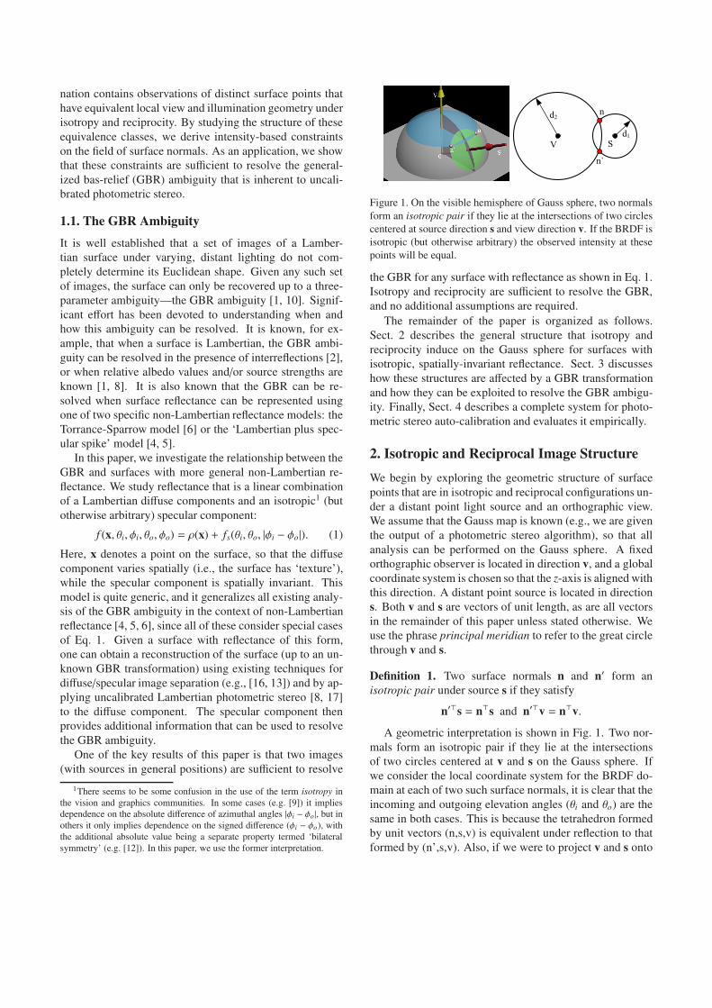
V S

n

n`

d2

d1

Figure 1. On the visible hemisphere of Gauss sphere, two normals

form an isotropic pair if they lie at the intersections of two circles

centered at source direction s and view direction v. If the BRDF is

isotropic (but otherwise arbitrary) the observed intensity at these

points will be equal.

the GBR for any surface with reflectance as shown in Eq. 1.

Isotropy and reciprocity are sufficient to resolve the GBR,

and no additional assumptions are required.

The remainder of the paper is organized as follows.

Sect. 2 describes the general structure that isotropy and

reciprocity induce on the Gauss sphere for surfaces with

isotropic, spatially-invariant reflectance. Sect. 3 discusses

how these structures are affected by a GBR transformation

and how they can be exploited to resolve the GBR ambigu-

ity. Finally, Sect. 4 describes a complete system for photo-

metric stereo auto-calibration and evaluates it empirically.

2. Isotropic and Reciprocal Image Structure

We begin by exploring the geometric structure of surface

points that are in isotropic and reciprocal configurations un-

der a distant point light source and an orthographic view.

We assume that the Gauss map is known (e.g., we are given

the output of a photometric stereo algorithm), so that all

analysis can be performed on the Gauss sphere. A fixed

orthographic observer is located in direction v, and a global

coordinate system is chosen so that the z-axis is aligned with

this direction. A distant point source is located in direction

s. Both v and s are vectors of unit length, as are all vectors

in the remainder of this paper unless stated otherwise. We

use the phrase principal meridian to refer to the great circle

through v and s.

Definition 1. Two surface normals n and n′ form an

isotropic pair under source s if they satisfy

n′⊤s = n⊤s and n′⊤v = n⊤v.

A geometric interpretation is shown in Fig. 1. Two nor-

mals form an isotropic pair if they lie at the intersections

of two circles centered at v and s on the Gauss sphere. If

we consider the local coordinate system for the BRDF do-

main at each of two such surface normals, it is clear that the

incoming and outgoing elevation angles (θi and θo) are the

same in both cases. This is because the tetrahedron formed

by unit vectors (n,s,v) is equivalent under reflection to that

formed by (n’,s,v). Also, if we were to project v and s onto

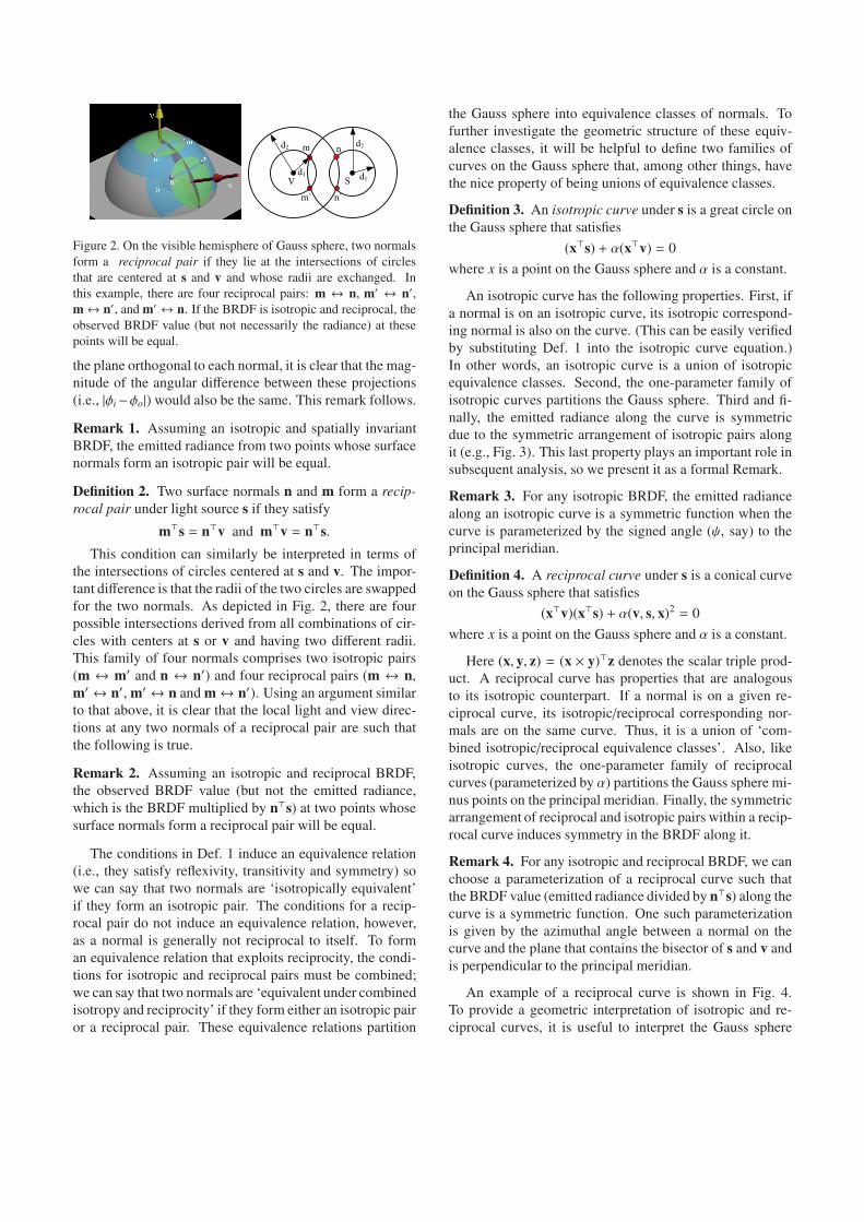
V S

m n

n`

d1

d2

d1

d2

m`

Figure 2. On the visible hemisphere of Gauss sphere, two normals

form a reciprocal pair if they lie at the intersections of circles

that are centered at s and v and whose radii are exchanged. In

this example, there are four reciprocal pairs: m ↔ n, m′ ↔ n′,

m↔ n′, and m′ ↔ n. If the BRDF is isotropic and reciprocal, the

observed BRDF value (but not necessarily the radiance) at these

points will be equal.

the plane orthogonal to each normal, it is clear that the mag-

nitude of the angular difference between these projections

(i.e., |φi−φo|) would also be the same. This remark follows.

Remark 1. Assuming an isotropic and spatially invariant

BRDF, the emitted radiance from two points whose surface

normals form an isotropic pair will be equal.

Definition 2. Two surface normals n and m form a recip-

rocal pair under light source s if they satisfy

m⊤s = n⊤v and m⊤v = n⊤s.

This condition can similarly be interpreted in terms of

the intersections of circles centered at s and v. The impor-

tant difference is that the radii of the two circles are swapped

for the two normals. As depicted in Fig. 2, there are four

possible intersections derived from all combinations of cir-

cles with centers at s or v and having two different radii.

This family of four normals comprises two isotropic pairs

(m ↔ m′ and n ↔ n′) and four reciprocal pairs (m ↔ n,

m′ ↔ n′, m′ ↔ n and m↔ n′). Using an argument similar

to that above, it is clear that the local light and view direc-

tions at any two normals of a reciprocal pair are such that

the following is true.

Remark 2. Assuming an isotropic and reciprocal BRDF,

the observed BRDF value (but not the emitted radiance,

which is the BRDF multiplied by n⊤s) at two points whose

surface normals form a reciprocal pair will be equal.

The conditions in Def. 1 induce an equivalence relation

(i.e., they satisfy reflexivity, transitivity and symmetry) so

we can say that two normals are ‘isotropically equivalent’

if they form an isotropic pair. The conditions for a recip-

rocal pair do not induce an equivalence relation, however,

as a normal is generally not reciprocal to itself. To form

an equivalence relation that exploits reciprocity, the condi-

tions for isotropic and reciprocal pairs must be combined;

we can say that two normals are ‘equivalent under combined

isotropy and reciprocity’ if they form either an isotropic pair

or a reciprocal pair. These equivalence relations partition

the Gauss sphere into equivalence classes of normals. To

further investigate the geometric structure of these equiv-

alence classes, it will be helpful to define two families of

curves on the Gauss sphere that, among other things, have

the nice property of being unions of equivalence classes.

Definition 3. An isotropic curve under s is a great circle on

the Gauss sphere that satisfies

(x⊤s) + α(x⊤v) = 0

where x is a point on the Gauss sphere and α is a constant.

An isotropic curve has the following properties. First, if

a normal is on an isotropic curve, its isotropic correspond-

ing normal is also on the curve. (This can be easily verified

by substituting Def. 1 into the isotropic curve equation.)

In other words, an isotropic curve is a union of isotropic

equivalence classes. Second, the one-parameter family of

isotropic curves partitions the Gauss sphere. Third and fi-

nally, the emitted radiance along the curve is symmetric

due to the symmetric arrangement of isotropic pairs along

it (e.g., Fig. 3). This last property plays an important role in

subsequent analysis, so we present it as a formal Remark.

Remark 3. For any isotropic BRDF, the emitted radiance

along an isotropic curve is a symmetric function when the

curve is parameterized by the signed angle (ψ, say) to the

principal meridian.

Definition 4. A reciprocal curve under s is a conical curve

on the Gauss sphere that satisfies

(x⊤v)(x⊤s) + α(v, s, x)2 = 0

where x is a point on the Gauss sphere and α is a constant.

Here (x, y, z) = (x × y)⊤z denotes the scalar triple prod-

uct. A reciprocal curve has properties that are analogous

to its isotropic counterpart. If a normal is on a given re-

ciprocal curve, its isotropic/reciprocal corresponding nor-

mals are on the same curve. Thus, it is a union of ‘com-

bined isotropic/reciprocal equivalence classes’. Also, like

isotropic curves, the one-parameter family of reciprocal

curves (parameterized by α) partitions the Gauss sphere mi-

nus points on the principal meridian. Finally, the symmetric

arrangement of reciprocal and isotropic pairs within a recip-

rocal curve induces symmetry in the BRDF along it.

Remark 4. For any isotropic and reciprocal BRDF, we can

choose a parameterization of a reciprocal curve such that

the BRDF value (emitted radiance divided by n⊤s) along the

curve is a symmetric function. One such parameterization

is given by the azimuthal angle between a normal on the

curve and the plane that contains the bisector of s and v and

is perpendicular to the principal meridian.

An example of a reciprocal curve is shown in Fig. 4.

To provide a geometric interpretation of isotropic and re-

ciprocal curves, it is useful to interpret the Gauss sphere

as being mapped to a plane. An elliptic plane is obtained

by a gnomonic (or central) projection that maps a point of

the sphere from the center of the sphere onto the tangent

plane at v. It maps a point to a point, a great circle to a

line, and a conical curve to a conic. The elliptic plane is a

real projective plane with an elliptic metric [3]. The three

great circles c1 = {x : v⊤x = 0}, c2 = {x : s⊤x = 0}, and

c3 = {x : (v × s)⊤x = 0} are mapped into three lines in the

elliptic plane: l1 is the line at infinity, l2 = s, and l3 = v × s.

On the elliptic plane, isotropic curves form a pencil (lin-

ear family) of lines by l1 and l2. Reciprocal curves form a

pencil of conics going through the double points p = l1 × l3(the intersection of l1 and l2) and q = l2× l3 (the intersection

of l1 and l2). The conic pencil is a linear family of parabola

directed by the light source direction s, and it touches the

point at infinity q.

3. Behavior under GBR Transformations

The isotropic and reciprocal structures described in the pre-

vious section exist whenever a curved surface is illuminated

from a distant point-source and viewed orthographically.

They provide constraints between the intensities observed

at distinct surface points and the orientation of the surface

normals at these points. Since these constraints are valid for

any isotropic and reciprocal BRDF, they may find use for a

variety of tasks.

In this section, we analyze the behavior of these struc-

tures when a GBR transformation is applied. We show

that, somewhat surprisingly, a GBR transformation gen-

erally maps isotropic/reciprocal curves ‘as sets’ to other

isotropic/reciprocal curves. At the same time, normals

within each curve generally move relative to one another,

thereby breaking the symmetry in the radiance functions

along the curve (see Figs. 3 and 4). As a result, given an

initial reconstruction up to an arbitrary GBR ambiguity, we

can establish the Euclidean reconstruction by finding the

GBR transformation that restores this symmetry structure.

3.1. GBR Transformations

Given three or more uncalibrated images of a Lambertian

surface, the field of surface normals n(x) (defined over the

image plane parameterized by x ∈ R2) and the source di-

rections si can only be recovered up to an invertible linear

transformation of R3 [8]. It has been shown that by impos-

ing integrability on the surface, this general linear transfor-

mation is restricted to lie in the group of GBR transforma-

tions, which are 3 × 3 matrices of the form [1]

G =

1 0 0

0 1 0

µ ν λ

,

with µ, ν, λ ∈ R. A GBR transformation affects the normal

field and source directions according to

n̄ = G−⊤n/||G−⊤n||, s̄ = Gs/||Gs||, (2)

andn = G⊤n̄/||G⊤n̄||, s = G−1s̄/||G−1s̄|| (3)

is the effect of the inverse transformation.

It is easy to verify that a GBR transformation affects nei-

ther view direction v nor the principal meridian. Isotropy

and reciprocity, however, are in general destroyed by the

GBR since n⊤s , n̄⊤s̄. As a result, if we are given a recon-

struction up to an unknown GBR transformation and we are

able to find the pairs of transformed isotropic and reciprocal

normals, we expect that the GBR can be solved.

A comment on terminology: in the subsequent discus-

sion, we will be interested in describing the manner in

which two normals n ↔ m of an isotropic or reciprocal

pair under s are affected by a GBR transformation. Since

a GBR transformation does not preserve isotropy and reci-

procity, we are generally uninterested in normals that form

isotropic/reciprocal pairs under s̄ in the sense of Defs. 1 and

2. Instead, we say that transformed normal n̄ corresponds

to transformed normal m̄ if the pre-images of these normals

n and m form an isotropic/reciprocal pair under s. The story

is different, however, for isotropic and reciprocal curves.

Since these curves are preserved as sets under a GBR trans-

formation, it does make sense to consider isotropic and re-

ciprocal curves under s̄ in the sense of Defs. 3 and 4.

3.2. Isotropy and GBR Transformations

We first look at the action of a GBR transformation on

isotropic pairs and isotropic curves.

Proposition 1. A GBR transformation maps each isotropic

curve under s ‘as a set’ to an isotropic curve under s̄.

To prove this, we first look at how a pair of isotropic nor-

mals is transformed by G. Suppose n̄ is a GBR-transformed

normal and x̄ is its unknown isotropic correspondence.

Since the pre-images of n̄ and x̄ form an isotropic pair un-

der s, we know x⊤v = n⊤v and x⊤s = n⊤s. By substituting

Eq. 3 into these equations, we obtain the following linear

constraint for the position of x̄ corresponding to n̄:

(x̄⊤s̄) + α(x̄⊤v̄) = 0,

withα = −(n̄⊤s̄)/(n̄⊤v̄).

Thus, if n and x form an isotropic pair under s, then n̄ and x̄

lie on an isotropic curve under s̄.

To complete the proof, we can explicitly derive a map-

ping between the pre-GBR and post-GBR isotropic curves

by substituting the inverse transformation equations (Eq. 3)

into the expression above. The yields the following equa-

tion for the pre-image of the isotropic curve:

(x⊤s) + β(x⊤v) = 0,

where β = α||Gs||/λ. This is also an isotropic curve, which

proves Proposition 1.

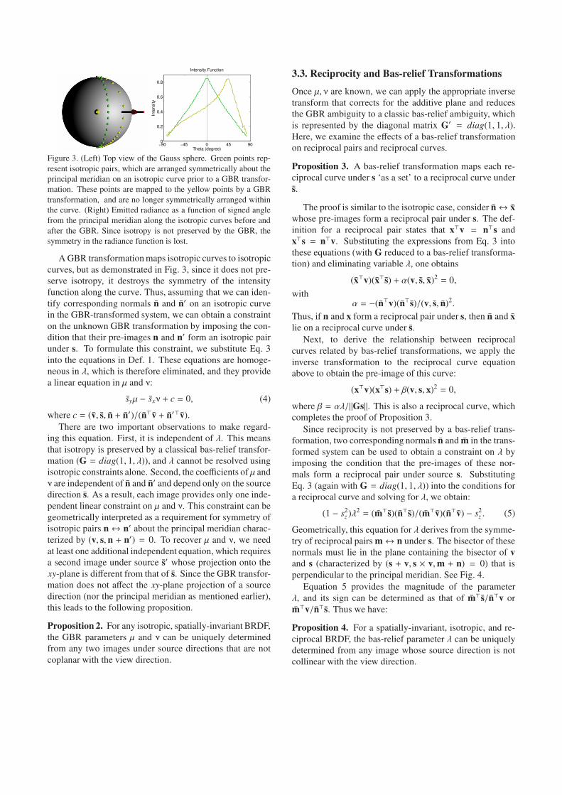
−90 −45 0 45 900

0.2

0.4

0.6

0.8

Theta (degree)In

ten

sity

Intensity Function

Figure 3. (Left) Top view of the Gauss sphere. Green points rep-

resent isotropic pairs, which are arranged symmetrically about the

principal meridian on an isotropic curve prior to a GBR transfor-

mation. These points are mapped to the yellow points by a GBR

transformation, and are no longer symmetrically arranged within

the curve. (Right) Emitted radiance as a function of signed angle

from the principal meridian along the isotropic curves before and

after the GBR. Since isotropy is not preserved by the GBR, the

symmetry in the radiance function is lost.

A GBR transformation maps isotropic curves to isotropic

curves, but as demonstrated in Fig. 3, since it does not pre-

serve isotropy, it destroys the symmetry of the intensity

function along the curve. Thus, assuming that we can iden-

tify corresponding normals n̄ and n̄′ on an isotropic curve

in the GBR-transformed system, we can obtain a constraint

on the unknown GBR transformation by imposing the con-

dition that their pre-images n and n′ form an isotropic pair

under s. To formulate this constraint, we substitute Eq. 3

into the equations in Def. 1. These equations are homoge-

neous in λ, which is therefore eliminated, and they provide

a linear equation in µ and ν:

s̄yµ − s̄xν + c = 0, (4)

where c = (v̄, s̄, n̄ + n̄′)/(n̄⊤v̄ + n̄′⊤v̄).

There are two important observations to make regard-

ing this equation. First, it is independent of λ. This means

that isotropy is preserved by a classical bas-relief transfor-

mation (G = diag(1, 1, λ)), and λ cannot be resolved using

isotropic constraints alone. Second, the coefficients of µ and

ν are independent of n̄ and n̄′ and depend only on the source

direction s̄. As a result, each image provides only one inde-

pendent linear constraint on µ and ν. This constraint can be

geometrically interpreted as a requirement for symmetry of

isotropic pairs n↔ n′ about the principal meridian charac-

terized by (v, s, n + n′) = 0. To recover µ and ν, we need

at least one additional independent equation, which requires

a second image under source s̄′ whose projection onto the

xy-plane is different from that of s̄. Since the GBR transfor-

mation does not affect the xy-plane projection of a source

direction (nor the principal meridian as mentioned earlier),

this leads to the following proposition.

Proposition 2. For any isotropic, spatially-invariant BRDF,

the GBR parameters µ and ν can be uniquely determined

from any two images under source directions that are not

coplanar with the view direction.

3.3. Reciprocity and Bas-relief Transformations

Once µ, ν are known, we can apply the appropriate inverse

transform that corrects for the additive plane and reduces

the GBR ambiguity to a classic bas-relief ambiguity, which

is represented by the diagonal matrix G′ = diag(1, 1, λ).

Here, we examine the effects of a bas-relief transformation

on reciprocal pairs and reciprocal curves.

Proposition 3. A bas-relief transformation maps each re-

ciprocal curve under s ‘as a set’ to a reciprocal curve under

s̄.

The proof is similar to the isotropic case, consider n̄↔ x̄

whose pre-images form a reciprocal pair under s. The def-

inition for a reciprocal pair states that x⊤v = n⊤s and

x⊤s = n⊤v. Substituting the expressions from Eq. 3 into

these equations (with G reduced to a bas-relief transforma-

tion) and eliminating variable λ, one obtains

(x̄⊤v)(x̄⊤s̄) + α(v, s̄, x̄)2 = 0,

withα = −(n̄⊤v)(n̄⊤s̄)/(v, s̄, n̄)2.

Thus, if n and x form a reciprocal pair under s, then n̄ and x̄

lie on a reciprocal curve under s̄.

Next, to derive the relationship between reciprocal

curves related by bas-relief transformations, we apply the

inverse transformation to the reciprocal curve equation

above to obtain the pre-image of this curve:

(x⊤v)(x⊤s) + β(v, s, x)2 = 0,

where β = αλ/||Gs||. This is also a reciprocal curve, which

completes the proof of Proposition 3.

Since reciprocity is not preserved by a bas-relief trans-

formation, two corresponding normals n̄ and m̄ in the trans-

formed system can be used to obtain a constraint on λ by

imposing the condition that the pre-images of these nor-

mals form a reciprocal pair under source s. Substituting

Eq. 3 (again with G = diag(1, 1, λ)) into the conditions for

a reciprocal curve and solving for λ, we obtain:

(1 − s2z )λ2 = (m̄⊤s̄)(n̄⊤s̄)/(m̄⊤v̄)(n̄⊤v̄) − s2

z . (5)

Geometrically, this equation for λ derives from the symme-

try of reciprocal pairs m↔ n under s. The bisector of these

normals must lie in the plane containing the bisector of v

and s (characterized by (s + v, s × v,m + n) = 0) that is

perpendicular to the principal meridian. See Fig. 4.

Equation 5 provides the magnitude of the parameter

λ, and its sign can be determined as that of m̄⊤s̄/n̄⊤v or

m̄⊤v/n̄⊤s̄. Thus we have:

Proposition 4. For a spatially-invariant, isotropic, and re-

ciprocal BRDF, the bas-relief parameter λ can be uniquely

determined from any image whose source direction is not

collinear with the view direction.

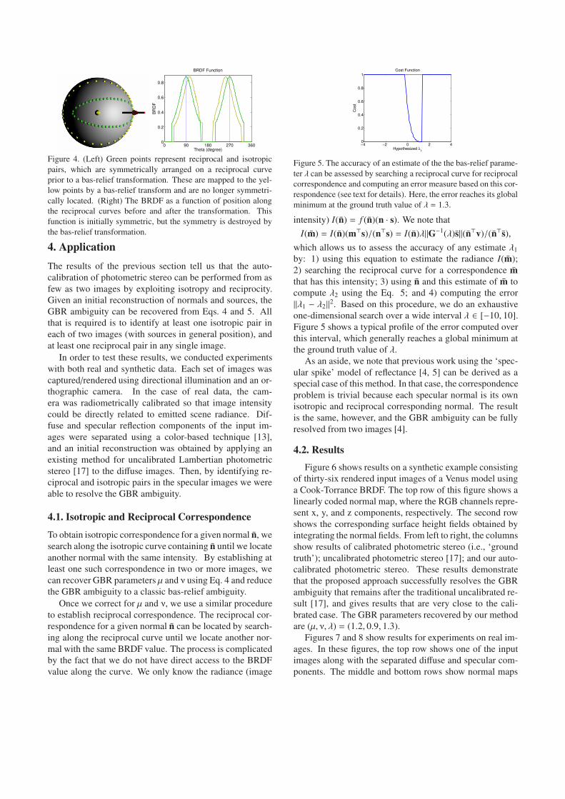
0 90 180 270 3600

0.2

0.4

0.6

0.8

Theta (degree)B

RD

F

BRDF Function

Figure 4. (Left) Green points represent reciprocal and isotropic

pairs, which are symmetrically arranged on a reciprocal curve

prior to a bas-relief transformation. These are mapped to the yel-

low points by a bas-relief transform and are no longer symmetri-

cally located. (Right) The BRDF as a function of position along

the reciprocal curves before and after the transformation. This

function is initially symmetric, but the symmetry is destroyed by

the bas-relief transformation.

4. Application

The results of the previous section tell us that the auto-

calibration of photometric stereo can be performed from as

few as two images by exploiting isotropy and reciprocity.

Given an initial reconstruction of normals and sources, the

GBR ambiguity can be recovered from Eqs. 4 and 5. All

that is required is to identify at least one isotropic pair in

each of two images (with sources in general position), and

at least one reciprocal pair in any single image.

In order to test these results, we conducted experiments

with both real and synthetic data. Each set of images was

captured/rendered using directional illumination and an or-

thographic camera. In the case of real data, the cam-

era was radiometrically calibrated so that image intensity

could be directly related to emitted scene radiance. Dif-

fuse and specular reflection components of the input im-

ages were separated using a color-based technique [13],

and an initial reconstruction was obtained by applying an

existing method for uncalibrated Lambertian photometric

stereo [17] to the diffuse images. Then, by identifying re-

ciprocal and isotropic pairs in the specular images we were

able to resolve the GBR ambiguity.

4.1. Isotropic and Reciprocal Correspondence

To obtain isotropic correspondence for a given normal n̄, we

search along the isotropic curve containing n̄ until we locate

another normal with the same intensity. By establishing at

least one such correspondence in two or more images, we

can recover GBR parameters µ and ν using Eq. 4 and reduce

the GBR ambiguity to a classic bas-relief ambiguity.

Once we correct for µ and ν, we use a similar procedure

to establish reciprocal correspondence. The reciprocal cor-

respondence for a given normal n̄ can be located by search-

ing along the reciprocal curve until we locate another nor-

mal with the same BRDF value. The process is complicated

by the fact that we do not have direct access to the BRDF

value along the curve. We only know the radiance (image

−4 −2 0 2 40

0.2

0.4

0.6

0.8

1

Hypothesized λ1

Cost

Cost Function

Figure 5. The accuracy of an estimate of the the bas-relief parame-

ter λ can be assessed by searching a reciprocal curve for reciprocal

correspondence and computing an error measure based on this cor-

respondence (see text for details). Here, the error reaches its global

minimum at the ground truth value of λ = 1.3.

intensity) I(n̄) = f (n̄)(n · s). We note that

I(m̄) = I(n̄)(m⊤s)/(n⊤s) = I(n̄)λ||G−1(λ)s̄||(n̄⊤v)/(n̄⊤s̄),

which allows us to assess the accuracy of any estimate λ1

by: 1) using this equation to estimate the radiance I(m̄);

2) searching the reciprocal curve for a correspondence m̄

that has this intensity; 3) using n̄ and this estimate of m̄ to

compute λ2 using the Eq. 5; and 4) computing the error

||λ1 − λ2||2. Based on this procedure, we do an exhaustive

one-dimensional search over a wide interval λ ∈ [−10, 10].

Figure 5 shows a typical profile of the error computed over

this interval, which generally reaches a global minimum at

the ground truth value of λ.

As an aside, we note that previous work using the ‘spec-

ular spike’ model of reflectance [4, 5] can be derived as a

special case of this method. In that case, the correspondence

problem is trivial because each specular normal is its own

isotropic and reciprocal corresponding normal. The result

is the same, however, and the GBR ambiguity can be fully

resolved from two images [4].

4.2. Results

Figure 6 shows results on a synthetic example consisting

of thirty-six rendered input images of a Venus model using

a Cook-Torrance BRDF. The top row of this figure shows a

linearly coded normal map, where the RGB channels repre-

sent x, y, and z components, respectively. The second row

shows the corresponding surface height fields obtained by

integrating the normal fields. From left to right, the columns

show results of calibrated photometric stereo (i.e., ‘ground

truth’); uncalibrated photometric stereo [17]; and our auto-

calibrated photometric stereo. These results demonstrate

that the proposed approach successfully resolves the GBR

ambiguity that remains after the traditional uncalibrated re-

sult [17], and gives results that are very close to the cali-

brated case. The GBR parameters recovered by our method

are (µ, ν, λ) = (1.2, 0.9, 1.3).

Figures 7 and 8 show results for experiments on real im-

ages. In these figures, the top row shows one of the input

images along with the separated diffuse and specular com-

ponents. The middle and bottom rows show normal maps

Figure 6. Results from thirty-six synthetic images rendered with

a Cook-Torrance BRDF. Top row: linearly coded normal maps,

where r, g, b channels represent x, y, z components. Bottom

row: surface height fields. Results in columns from left to right:

calibrated lighting directions; traditional uncalibrated photomet-

ric stereo [17]; our auto-calibrated photometric stereo algorithm,

which successfully resolves the GBR ambiguity and obtains re-

sults comparable to the calibrated case.

Ground truth s Results from [17] Auto-calibrated s Error

(0.34, 0.26, 0.90) (0.13, 0.20, -0.97) (0.33, 0.52, 0.79) 16

(0.35, -0.30, 0.89) (0.20, -0.07, -0.98) (0.39, -0.15, 0.90) 8

(-0.27, -0.34, 0.90) (-0.02, 0.05, -0.99) (-0.07, 0.19, 0.98) 33

(-0.23, 0.11, 0.97) (-0.02, 0.03, -0.99) (-0.05, 0.11, 0.99) 10

Table 1. Accuracy of recovered source directions for four images

of the pear dataset. Right-most column shows angular error.

and surface height fields as before, with columns from left

to right representing: 1) calibrated Lambertian photometric

stereo applied to the diffuse images; 2) uncalibrated Lam-

bertian photometric stereo [17] applied to the diffuse im-

ages; and 3) our auto-calibrated results that use the specular

images to resolve the GBR ambiguity. For the calibrated

case, we use source directions that were measured from

mirrored spheres during acquisition. The GBR parameters

(µ, ν, λ) recovered by our method are (2.1,−1.2,−3.3) and

(−2,−1.2, 3.1) for the pear and fish, respectively.

Table 1 and Figure 9 provide quantitative evaluation re-

sults. For the pear data, Table 1 compares the source direc-

tions recovered by our method to the ground-truth source di-

rections measured during acquisition. Here, the right-most

column provides angular error in degrees. Figure 9 shows

average angular errors between the normals recovered using

our approach and those recovered using calibrated photo-

metric stereo with the measured source directions. For the

Venus, pear and fish examples, our method achieves aver-

age angular errors of 2.8, 4 and 6.7 degrees and maximum

angular errors of 44, 32 and 26.3 degrees, respectively. The

sources of error include: 1) inaccuracies in isotropic and

reciprocal correspondence; 2) imaging noise; and 3) inac-

curate diffuse/specular separation.

Figure 7. Results from four input images of a pear. Top row:

one input image with separated diffuse and specular components.

Middle row: linearly encoded normal map. Bottom row: surface

height fields. Columns from left to right show photometric stereo

results using: calibrated lighting directions; an uncalibrated ap-

proach [17]; and our auto-calibrated approach that resolves the

GBR and provides results comparable to the calibrated case.

Figure 8. Results from seven input images of a plastic toy fish. Top

row: one input image with separated diffuse and specular compo-

nents. Middle row: linearly encoded normal map. Bottom row:

surface height fields. Columns from left to right show photometric

stereo results using: calibrated lighting directions; an uncalibrated

approach [17]; and our auto-calibrated approach that resolves the

GBR and provides results comparable to the calibrated case.

Finally, Fig. 10 shows surfaces obtained by integrat-

ing the recovered normal fields from the calibrated, uncali-

brated, and auto-calibrated methods. In each case, our auto-

calibrated procedure significantly improves the uncalibrated

results by resolving the GBR ambiguity.

Figure 9. Surface normal angular error between the results of our

auto-calibrated method and calibrated photometric stereo results.

Figure 10. Surfaces recovered from integrating estimated normal

fields. Rendering of the recovered surfaced from a novel view

point. Columns from left to right show photometric stereo re-

sults using: calibrated lighting directions; an uncalibrated ap-

proach [17]; and our auto-calibrated approach.

5. Conclusion

This paper demonstrates that the generalized bas-relief

ambiguity can be resolved for any surface that has an

additive specular reflectance component that is spatially-

invariant, isotropic and reciprocal. It shows that two images

are sufficient to resolve the GBR, and presents a practical

algorithm for doing so. The result is an auto-calibrating

system for photometric stereo that can be applied to a very

wide variety of surfaces.

More broadly, this paper demonstrates the utility of

two very general reflectance properties: isotropy and reci-

procity. It shows that any image of a surface (convex or

not) under directional illumination and orthographic view

contains observations of distinct surface points that are in

isotropic and reciprocal configurations. By analyzing these

equivalence classes, it reveals patterns of intensity on the

Gauss sphere that can be used as constraints on surface ge-

ometry. In the future, these constraints could potentially be

used in other ways for the analysis of scenes with complex,

non-Lambertian surfaces.

6. Acknowledgements

P. Tan and L. Quan were supported by Hong Kong

RGC project 619005, 619006 and RGC/NSFC project

N HKUST602/05. T. Zickler was supported by NSF CA-

REER Award IIS-0546408. D. Kriegman and S. Mallick

were partially supported under NSF grants IIS-0308185 and

NSFEIA-0303622.

References

[1] P. N. Belhumeur, D. J. Kriegman, and A. L. Yuille. The bas-

relief ambiguity. IJCV, 35(1):33–44, 1999.

[2] M. K. Chandraker, F. Kahl, and D. Kriegman. Reflections on

the generalized bas-relief ambiguity. In CVPR, 2005.

[3] H. S. M. Coxeter. Introduction to Geometry, 2nd Edition.

Wiley, 1989.

[4] O. Drbohlav and M. Chantler. Can two specular pixels cal-

ibrate photometric stereo? In ICCV, volume 2, pages 850–

1857, 2005.

[5] O. Drbohlav and R. Sara. Specularities reduce ambiguity of

uncalibrated photometric stereo. In ECCV, volume 2, pages

46–60, 2002.

[6] A. S. Georghiades. Incorporating the Torrance and Sparrow

model of reflectance in uncalibrated photometric stereo. In

ICCV, pages 816–823, 2003.

[7] T. Hawkins and P. E. P. Debevec. A dual light stage. In

Rendering Techniques 2005 (Proc. Eurographics Symposium

on Rendering), 2005.

[8] K. Hayakawa. Photometric stereo under a light source with

arbitrary motion. J. Opt Soc. Am., 11(11), 1994.

[9] J. J. Koenderink and A. J. van Doorn. Phenomenologi-

cal description of bidirectional surface reflection. JOSA A,

15:2903–2912, 1998.

[10] D. J. Kriegman and P. N. Belhumeur. What shadows reveal

about object structure. JOSA A, 18, 2001.

[11] J. Lu and J. Little. Reflectance and shape from images using

a collinear light source. IJCV, 32(3):1–28, 1999.

[12] S. R. Marschner. Inverse rendering for computer graphics.

PhD thesis, Cornell University, 1998.

[13] Y. Sato and K. Ikeuchi. Temporal-color space analysis

of reflection. Journal of Optical Society of America A,

11(11):2990 – 3002, November 1994.

[14] P. Sen, B. Chen, G. Garg, S. Marschner, M. Horowitz,

M. Levoy, and H. P. A. Lensch. Dual photography. In ACM

Transactions on Graphics (ACM SIGGRAPH), 2005.

[15] S. Shafer. Using color to separate reflection components.

COLOR research and applications, 10(4):210–218, 1985.

[16] R. T. Tan and K. Ikeuchi. Separating reflection components

of textured surfaces using a single image. PAMI, 27:178–

193, 2005.

[17] A. L. Yuille and D. Snow. Shape and albedo from multiple

images uing integrability. In CVPR, pages 158–164, 1997.

[18] T. Zickler, P. Belhumeur, and D. Kriegman. Helmholtz

stereopsis: Exploiting reciprocity for surface reconstruction.

IJCV, 49(2/3):215–227, September 2002.