Isotropic PCA and Affine-Invariant Clustering

S. Charles Brubaker∗ Santosh S. Vempala∗

Abstract

We present an extension of Principal Component Analysis (PCA) and a new algorithm forclustering points in Rn based on it. The key property of the algorithm is that it is affine-invariant.When the input is a sample from a mixture of two arbitrary Gaussians, the algorithm correctlyclassifies the sample assuming only that the two components are separable by a hyperplane,i.e., there exists a halfspace that contains most of one Gaussian and almost none of the otherin probability mass. This is nearly the best possible, improving known results substantially[14, 9, 1]. For k > 2 components, the algorithm requires only that there be some (k − 1)-dimensional subspace in which the overlap in every direction is small. Here we define overlap tobe the ratio of the following two quantities: 1) the average squared distance between a point andthe mean of its component, and 2) the average squared distance between a point and the mean ofthe mixture. The main result may also be stated in the language of linear discriminant analysis:if the standard Fisher discriminant [8] is small enough, labels are not needed to estimate theoptimal subspace for projection. Our main tools are isotropic transformation, spectral projectionand a simple reweighting technique. We call this combination isotropic PCA.

∗College of Computing, Georgia Tech. Email: brubaker,vempala@cc.gatech.edu

1 Introduction

We present an extension to Principal Component Analysis (PCA), which is able to go beyondstandard PCA in identifying “important” directions. When the covariance matrix of the input(distribution or point set in Rn) is a multiple of the identity, then PCA reveals no information; thesecond moment along any direction is the same. Such inputs are called isotropic. Our extension,which we call isotropic PCA, can reveal interesting information in such settings. We use thistechnique to give an affine-invariant clustering algorithm for points in Rn. When applied to theproblem of unraveling mixtures of arbitrary Gaussians from unlabeled samples, the algorithm yieldssubstantial improvements of known results.

To illustrate the technique, consider the uniform distribution on the set X = (x, y) ∈ R2 : x ∈−1, 1, y ∈ [−

√3,√

3], which is isotropic. Suppose this distribution is rotated in an unknownway and that we would like to recover the original x and y axes. For each point in a sample, wemay project it to the unit circle and compute the covariance matrix of the resulting point set. Thex direction will correspond to the greater eigenvector, the y direction to the other. See Figure 1 foran illustration. Instead of projection onto the unit circle, this process may also be thought of asimportance weighting, a technique which allows one to simulate one distribution with another. Inthis case, we are simulating a distribution over the set X, where the density function is proportionalto (1 + y2)−1, so that points near (1, 0) or (−1, 0) are more probable.

−2.5 −2 −1.5 −1 −0.5 0 0.5 1 1.5 2 2.5−2

−1.5

−1

−0.5

0

0.5

1

1.5

2

a

a’

Figure 1: Mapping points to the unit circle and then finding the direction of maximum variancereveals the orientation of this isotropic distribution.

In this paper, we describe how to apply this method to mixtures of arbitrary Gaussians in Rn

in order to find a set of directions along which the Gaussians are well-separated. These directionsspan the Fisher subspace of the mixture, a classical concept in Pattern Recognition. Once thesedirections are identified, points can be classified according to which component of the distributiongenerated them, and hence all parameters of the mixture can be learned.

What separates this paper from previous work on learning mixtures is that our algorithm isaffine-invariant. Indeed, for every mixture distribution that can be learned using a previouslyknown algorithm, there is a linear transformation of bounded condition number that causes thealgorithm to fail. For k = 2 components our algorithm has nearly the best possible guarantees (andsubsumes all previous results) for clustering Gaussian mixtures. For k > 2, it requires that therebe a (k − 1)-dimensional subspace where the overlap of the components is small in every direction(See section 1.2). This condition can be stated in terms of the Fisher discriminant, a quantitycommonly used in the field of Pattern Recognition with labeled data. Because our algorithm isaffine invariant, it makes it possible to unravel a much larger set of Gaussian mixtures than had

1

been possible previously.The first step of our algorithm is to place the mixture in isotropic position (see Section 1.2) via

an affine transformation. This has the effect of making the (k−1)-dimensional Fisher subspace, i.e.,the one that minimizes the Fisher discriminant, the same as the subspace spanned by the means ofthe components (they only coincide in general in isotropic position), for any mixture. The rest ofthe algorithm identifies directions close to this subspace and uses them to cluster, without access tolabels. Intuitively this is hard since after isotropy, standard PCA reveals no additional information.Before presenting the ideas and guarantees in more detail, we describe relevant related work.

1.1 Previous Work

A mixture model is a convex combination of distributions of known type. In the most commonlystudied version, a distribution F in Rn is composed of k unknown Gaussians. That is,

F = w1N(µ1,Σ1) + . . . + wkN(µk,Σk),

where the mixing weights wi, means µi, and covariance matrices Σi are all unknown. Typically,k n, so that a concise model explains a high dimensional phenomenon. A random sample isgenerated from F by first choosing a component with probability equal to its mixing weight andthen picking a random point from that component distribution. In this paper, we study the classicalproblem of unraveling a sample from a mixture, i.e., labeling each point in the sample accordingto its component of origin.

Heuristics for classifying samples include “expectation maximization” [5] and “k-means cluster-ing” [11]. These methods can take a long time and can get stuck with suboptimal classifications.Over the past decade, there has been much progress on finding polynomial-time algorithms withrigorous guarantees for classifying mixtures, especially mixtures of Gaussians [4, 15, 14, 17, 9, 1].Starting with Dasgupta’s paper [4], one line of work uses the concentration of pairwise distancesand assumes that the components’ means are so far apart that distances between points from thesame component are likely to be smaller than distances from points in different components. Aroraand Kannan [14] establish nearly optimal results for such distance-based algorithms. Unfortunatelytheir results inherently require separation that grows with the dimension of the ambient space andthe largest variance of each component Gaussian.

To see why this is unnatural, consider k well-separated Gaussians in Rk with means e1, . . . , ek,i.e. each mean is 1 unit away from the origin along a unique coordinate axis. Adding extradimensions with arbitrary variance does not affect the separability of these Gaussians, but thesealgorithms are no longer guaranteed to work. For example, suppose that each Gaussian has amaximum variance of ε 1. Then, adding O∗(kε−2) extra dimensions with variance ε will violatethe necessary separation conditions.

To improve on this, a subsequent line of work uses spectral projection (PCA). Vempala andWang [17] showed that for a mixture of spherical Gaussians, the subspace spanned by the top kprincipal components of the mixture contains the means of the components. Thus, projecting tothis subspace has the effect of shrinking the components while maintaining the separation betweentheir means. This leads to a nearly optimal separation requirement of

‖µi − µj‖ ≥ Ω(k1/4) maxσi, σj

where µi is the mean of component i and σ2i is the variance of component i along any direction.

Note that there is no dependence on the dimension of the distribution. Kannan et al. [9] applied thespectral approach to arbitrary mixtures of Gaussians (and more generally, logconcave distributions)

2

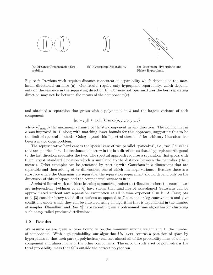
(a) Distance Concentration Sep-arability

(b) Hyperplane Separability (c) Intermean Hyperplane andFisher Hyperplane.

Figure 2: Previous work requires distance concentration separability which depends on the max-imum directional variance (a). Our results require only hyperplane separability, which dependsonly on the variance in the separating direction(b). For non-isotropic mixtures the best separatingdirection may not be between the means of the components(c).

and obtained a separation that grows with a polynomial in k and the largest variance of eachcomponent:

‖µi − µj‖ ≥ poly(k) maxσi,max, σj,max

where σ2i,max is the maximum variance of the ith component in any direction. The polynomial in

k was improved in [1] along with matching lower bounds for this approach, suggesting this to bethe limit of spectral methods. Going beyond this “spectral threshold” for arbitrary Gaussians hasbeen a major open problem.

The representative hard case is the special case of two parallel “pancakes”, i.e., two Gaussiansthat are spherical in n−1 directions and narrow in the last direction, so that a hyperplane orthogonalto the last direction separates the two. The spectral approach requires a separation that grows withtheir largest standard deviation which is unrelated to the distance between the pancakes (theirmeans). Other examples can be generated by starting with Gaussians in k dimensions that areseparable and then adding other dimensions, one of which has large variance. Because there is asubspace where the Gaussians are separable, the separation requirement should depend only on thedimension of this subspace and the components’ variances in it.

A related line of work considers learning symmetric product distributions, where the coordinatesare independent. Feldman et al [6] have shown that mixtures of axis-aligned Gaussians can beapproximated without any separation assumption at all in time exponential in k. A. Dasguptaet al [3] consider heavy-tailed distributions as opposed to Gaussians or log-concave ones and giveconditions under which they can be clustered using an algorithm that is exponential in the numberof samples. Chaudhuri and Rao [2] have recently given a polynomial time algorithm for clusteringsuch heavy tailed product distributions.

1.2 Results

We assume we are given a lower bound w on the minimum mixing weight and k, the numberof components. With high probability, our algorithm Unravel returns a partition of space byhyperplanes so that each part (a polyhedron) encloses almost all of the probability mass of a singlecomponent and almost none of the other components. The error of such a set of polyhedra is thetotal probability mass that falls outside the correct polyhedron.

3

We first state our result for two Gaussians in a way that makes clear the relationship to previouswork that relies on separation.

Theorem 1. Let w1, µ1,Σ1 and w2, µ2,Σ2 define a mixture of two Gaussians. There is an absoluteconstant C such that, if there exists a direction v such that

|projv(µ1 − µ2)| ≥ C(√

vT Σ1v +√

vT Σ2v)

w−2 log1/2

(1

wδ+

1η

),

then with probability 1 − δ algorithm Unravel returns two complementary halfspaces that haveerror at most η using time and a number of samples that is polynomial in n, w−1, log(1/δ).

The requirement is that in some direction the separation between the means must be compa-rable to the standard deviation. This separation condition of Theorem 1 is affine-invariant andmuch weaker than conditions of the form ‖µ1 − µ2‖ & maxσ1,max, σ2,max used in previous work.See Figure 2(a). The dotted line shows how previous work effectively treats every component asspherical. Hyperplane separability (Figure 2(b)) is a weaker condition. We also note that theseparating direction does not need to be the intermean direction as illustrated in Figure 2(c). Thedotted line illustrates hyperplane induced by the intermean direction, which may be far from theoptimal separating hyperplane shown by the solid line.

It will be insightful to state this result in terms of the Fisher discriminant, a standard notionfrom Pattern Recognition [8, 7] that is used with labeled data. In words, the Fisher discriminantalong direction p is

J(p) =the intra-component variance in direction p

the total variance in direction p

Mathematically, this is expressed as

J(p) =E[‖projp(x− µ`(x))‖2

]E[‖projp(x)‖2

] =pT (w1Σ1 + w2Σ2)p

pT (w1(Σ1 + µ1µT1 ) + w2(Σ2 + µ2µT

2 ))p

for x distributed according to a mixture distribution with means µi and covariance matrices Σi.We use `(x) to indicate the component from which x was drawn.

Theorem 2. There is an absolute constant C for which the following holds. Suppose that F is amixture of two Gaussians such that there exists a direction p for which

J(p) ≤ Cw3 log−1

(1

δw+

1η

).

With probability 1− δ, algorithm Unravel returns a halfspace with error at most η using time andsample complexity polynomial in n, w−1, log(1/δ).

There are several ways of generalizing the Fisher discriminant for k = 2 components to greaterk [7]. These generalizations are most easily understood when the distribution is isotropic. Anisotropic distribution has the identity matrix as its covariance and the origin as its mean. Anisotropic mixture therefore has

k∑i=1

wiµi = 0 andk∑

i=1

wi(Σi + µiµTi ) = I.

4

It is well known that any distribution with bounded covariance matrix (and therefore any mixture)can be made isotropic by an affine transformation. As we will see shortly, for k = 2, for an isotropicmixture, the line joining the means is the direction that minimizes the Fisher discriminant.

Under isotropy, the denominator of the Fisher discriminant is always 1. Thus, the discriminantis just the expected squared distance between the projection of a point and the projection of itsmean, where projection is onto some direction p. The generalization to k > 2 is natural, as we maysimply replace projection onto direction p with projection onto a (k − 1)-dimensional subspace S.For convenience, let

Σ =k∑

i=1

wiΣi.

Let the vector p1, . . . , pk−1 be an orthonormal basis of S and let `(x) be the component from whichx was drawn. We then have under isotropy

J(S) = E[‖projS(x− µ`(x))‖2] =k−1∑j=1

pTj Σpj

for x distributed according to a mixture distribution with means µi and covariance matrices Σi.As Σ is symmetric positive definite, it follows that the smallest k− 1 eigenvectors of the matrix areoptimal choices of pj and S is the span of these eigenvectors.

This motivates our definition of the Fisher subspace for any mixture with bounded secondmoments (not necessarily Gaussians).

Definition 1. Let wi, µi,Σi be the weights, means, and covariance matrices for an isotropic 1

mixture distribution with mean at the origin and where dim(spanµ1, . . . , µk) = k− 1. Let `(x) bethe component from which x was drawn. The Fisher subspace F is defined as the (k−1)-dimensionalsubspace that minimizes

J(S) = E[‖projS(x− µ`(x))‖2].

over subspaces S of dimension k − 1.

Note that dim(spanµ1, . . . , µk) is only k − 1 because isotropy implies∑k

i=1 wiµi = 0. Thenext lemma provides a simple alternative characterization of the Fisher subspace as the span of themeans of the components (after transforming to isotropic position). The proof is given in Section3.2.

Lemma 1. Suppose wi, µi,Σiki=1 defines an isotropic mixture in Rn. Let λ1 ≥ . . . ≥ λn be the

eigenvalues of the matrix Σ =∑k

i=1 wiΣi and let v1, . . . , vn be the corresponding eigenvectors. Ifthe dimension of the span of the means of the components is k − 1, then the Fisher subspace

F = spanvn−k+2, . . . , vn = spanµ1, . . . , µk.

Our algorithm attempts to find the Fisher subspace (or one close to it) and succeeds in doingso, provided the discriminant is small enough.

The next definition will be useful in stating our main theorem precisely.

1For non-isotropic mixtures, the Fisher discriminant generalizes toPk−1

j=1 pTj

“Pki=1 wi(Σi + µiµ

Ti )

”−1

Σpj and the

overlap to pT“Pk

i=1 wi(Σi + µiµTi )

”−1

Σp

5

Definition 2. The overlap of a mixture given as in Definition 1 is

φ = minS:dim(S)=k−1

maxp∈S

pT Σp. (1)

It is a direct consequence of the Courant-Fisher min-max theorem that φ is the (k−1)th smallesteigenvalue of the matrix Σ and the subspace achieving φ is the Fisher subspace, i.e.,

φ =∥∥E[projF (x− µ`(x))projF (x− µ`(x))

T ]∥∥

2.

We can now state our main theorem for k > 2.

Theorem 3. There is an absolute constant C for which the following holds. Suppose that F is amixture of k Gaussian components where the overlap satisfies

φ ≤ Cw3k−3 log−1

(nk

δw+

1η

)With probability 1− δ, algorithm Unravel returns a set of k polyhedra that have error at most ηusing time and a number of samples that is polynomial in n, w−1, log(1/δ).

In words, the algorithm successfully unravels arbitrary Gaussians provided there exists a (k−1)-dimensional subspace in which along every direction, the expected squared distance of a point toits component mean is smaller than the expected squared distance to the overall mean by roughly apoly(k, 1/w) factor. There is no dependence on the largest variances of the individual components,and the dependence on the ambient dimension is logarithmic. This means that the addition ofextra dimensions (even where the distribution has large variance) as discussed in Section 1.1 haslittle impact on the success of our algorithm.

2 Algorithm

The algorithm has three major components: an initial affine transformation, a reweighting step,and identification of a direction close to the Fisher subspace and a hyperplane orthogonal to thisdirection which leaves each component’s probability mass almost entirely in one of the halfspacesinduced by the hyperplane. The key insight is that the reweighting technique will either cause themean of the mixture to shift in the intermean subspace, or cause the top k−1 principal componentsof the second moment matrix to approximate the intermean subspace. In either case, we obtain adirection along which we can partition the components.

We first find an affine transformation W which when applied to F results in an isotropicdistribution. That is, we move the mean to the origin and apply a linear transformation to makethe covariance matrix the identity. We apply this transformation to a new set of m1 points xifrom F and then reweight according to a spherically symmetric Gaussian exp(−‖x‖2/(2α)) forα = Θ(n/w). We then compute the mean u and second moment matrix M of the resulting set. 2

After the reweighting, the algorithm chooses either the new mean or the direction of maximumsecond moment and projects the data onto this direction h. By bisecting the largest gap betweenpoints, we obtain a threshold t, which along with h defines a hyperplane that separates the com-ponents. Using the notation Hh,t = x ∈ Rn : hT x ≥ t, to indicate a halfspace, we then recurse

2This practice of transforming the points and then looking at the second moment matrix can be viewed as a formof kernel PCA; however the connection between our algorithm and kernel PCA is superficial. Our transformationdoes not result in any standard kernel. Moreover, it is dimension-preserving (it is just a reweighting), and hence the“kernel trick” has no computational advantage.

6

on each half of the mixture. Thus, every node in the recursion tree represents an intersection ofhalf-spaces. To make our analysis easier, we assume that we use different samples for each stepof the algorithm. The reader might find it useful to read Section 2.1, which gives an intuitiveexplaination for how the algorithm works on parallel pancakes, before reviewing the details of thealgorithm.

Algorithm 1 UnravelInput: Integer k, scalar w. Initialization: P = Rn.

1. (Isotropy) Use samples lying in P to compute an affine transformation W that makes thedistribution nearly isotropic (mean zero, identity covariance matrix).

2. (Reweighting) Use m1 samples in P and for each compute a weight e−‖x‖2/(α) (where α >

n/w).

3. (Separating Direction) Find the mean of the reweighted data µ. If ‖µ‖ >√

w/(32α), leth = µ. Otherwise, find the covariance matrix M of the reweighted points and let h be its topprincipal component.

4. (Recursion) Project m2 sample points to h and find the largest gap between points in theinterval [−1/2, 1/2]. If this gap is less than 1/4(k− 1), then return P . Otherwise, set t to bethe midpoint of the largest gap, recurse on P ∩Hh,t and P ∩H−h,−t, and return the union ofthe polyhedra produces by these recursive calls.

2.1 Parallel Pancakes

The following special case, which represents the open problem in previous work, will illuminate theintuition behind the new algorithm. Suppose F is a mixture of two spherical Gaussians that arewell-separated, i.e. the intermean distance is large compared to the standard deviation along anydirection. We consider two cases, one where the mixing weights are equal and another where theyare imbalanced.

After isotropy is enforced, each component will become thin in the intermean direction, givingthe density the appearance of two parallel pancakes. When the mixing weights are equal, the meansof the components will be equally spaced at a distance of 1− φ on opposite sides of the origin. Forimbalanced weights, the origin will still lie on the intermean direction but will be much closer tothe heavier component, while the lighter component will be much further away. In both cases, thistransformation makes the variance of the mixture 1 in every direction, so the principal componentsgive us no insight into the inter-mean direction.

Consider next the effect of the reweighting on the mean of the mixture. For the case of equalmixing weights, symmetry assures that the mean does not shift at all. For imbalanced weights,however, the heavier component, which lies closer to the origin will become heavier still. Thus,the reweighted mean shifts toward the mean of the heavier component, allowing us to detect theintermean direction.

Finally, consider the effect of reweighting on the second moments of the mixture with equalmixing weights. Because points closer to the origin are weighted more, the second moment in everydirection is reduced. However, in the intermean direction, where part of the moment is due tothe displacement of the component means from the origin, it shrinks less. Thus, the direction ofmaximum second moment is the intermean direction.

7

2.2 Overview of Analysis

To analyze the algorithm, in the general case, we will proceed as follows. Section 3 shows that underisotropy the Fisher subspace coincides with the intermean subspace (Lemma 1), gives the necessarysampling convergence and perturbation lemmas and relates overlap to a more conventional notionof separation (Prop. 5). Section 3.3 gives approximations to the first and second moments. Section4 then combines these approximations with the perturbation lemmas to show that the vector h(either the mean shift or the largest principal component) lies close to the intermean subspace.Finally, Section 5 shows the correctness of the recursive aspects of the algorithm.

3 Preliminaries

3.1 Matrix Properties

For a matrix Z, we will denote the ith largest eigenvalue of Z by λi(Z) or just λi if the matrix isclear from context. Unless specified otherwise, all norms are the 2-norm. For symmetric matrices,this is ‖Z‖2 = λ1(Z) = maxx∈Rn ‖Zx‖2/‖x‖2.

The following two facts from linear algebra will be useful in our analysis.

Fact 2. Let λ1 ≥ . . . ≥ λn be the eigenvalues for an n-by-n symmetric positive definite matrix Zand let v1, . . . vn be the corresponding eigenvectors. Then

λn + . . . + λn−k+1 = minS:dim(S)=k

k∑j=1

pTj Zpj ,

where pj is any orthonormal basis for S. If λn−k > λn−k+1, then spanvn, . . . , vn−k+1 is theunique minimizing subspace.

Recall that a matrix Z is positive semi-definite if xT Zx ≥ 0 for all non-zero x.

Fact 3. Suppose that the matrix

Z =[

A BT

B D

]is symmetric positive semi-definite and that A and D are square submatrices. Then ‖B‖ ≤√‖A‖‖D‖.

Proof. Let y and x be the top left and right singular vectors of B, so that yT Bx = ‖B‖. BecauseZ is positive semi-definite, we have that for any real γ,

0 ≤ [γxT yT ]Z[γxT yT ]T = γ2xT Ax + 2γyT Bx + yT Dy.

This is a quadratic polynomial in γ that can have only one real root. Therefore the discriminantmust be non-positive:

0 ≥ 4(yT Bx)2 − 4(xT Ax)(yT Dy).

We conclude that‖B‖ = yT Bx ≤

√(xT Ax)(yT Dy) ≤

√‖A‖‖D‖.

8

3.2 The Fisher Criterion and Isotropy

We begin with the proof of the lemma that for an isotropic mixture the Fisher subspace is the sameas the intermean subspace.

Proof of Lemma 1. By Definition 1 for an isotropic distribution, the Fisher subspace minimizes

J(S) = E[‖projS(x− µ`(x))‖2] =k−1∑j=1

pTj Σpj ,

where pj is an orthonormal basis for S.By Fact 2, one minimizing subspace is the span of the smallest k− 1 eigenvectors of the matrix

Σ, i.e. vn−k+2, . . . , vn. Because the distribution is isotropic,

Σ = I −k∑

i=1

wiµiµTi .

and these vectors become the largest eigenvectors of∑k

i=1 wiµiµTi . Clearly, spanvn−k+2, . . . , vn ⊆

spanµ1, . . . , µk, but both spans have dimension k− 1 making them equal. This also implies that

1− λn−k+2(Σ) = vTn−k+2

k∑i=1

wiµiµTi vn−k+2 > 0.

Thus, λn−k+2(Σ) < 1. On the other hand vn−k+1, must be orthogonal every µi, so λn−k+1(Σ) = 1.Therefore, λn−k+1(Σ) > λn−k+2(Σ) and by Fact 2 spanvn−k+2, . . . , vn = spanµ1, . . . , µk is theunique minimizing subspace.

It follows directly that under the conditions of Lemma 1, the overlap may be characterized as

φ = λn−k+2 (Σ) = 1− λk−1

(k∑

i=1

wiµiµTi

).

For clarity of the analysis, we will assume that Step 1 of the algorithm produces a perfectlyisotropic mixture. Theorem 4 gives a bound on the required number of samples to make thedistribution nearly isotropic, and as our analysis shows, our algorithm is robust to small estimationerrors.

We will also assume for convenience of notation that the the unit vectors along the first k−1 coor-dinate axes e1, . . . ek−1 span the intermean (i.e. Fisher) subspace. That is, F = spane1, . . . , ek−1.When considering this subspace it will be convenient to be able to refer to projection of the meanvectors to this subspace. Thus, we define µi ∈ Rk−1 to be the first k − 1 coordinates of µi; theremaining coordinates are all zero. In other terms,

µi = [Ik−1 0]µi .

In this coordinate system the covariance matrix of each component has a particular structure,which will be useful for our analysis. For the rest of this paper we fix the following notation: anisotropic mixture is defined by wi, µi,Σi. We assume that spane1, . . . , ek−1 is the intermeansubspace and Ai,Bi, and Di are defined such that

wiΣi =[

Ai BTi

Bi Di

](2)

where Ai is a (k − 1)× (k − 1) submatrix and Di is a (n− k + 1)× (n− k + 1) submatrix.

9

Lemma 4 (Covariance Structure). Using the above notation,

‖Ai‖ ≤ φ , ‖Di‖ ≤ 1 , ‖Bi‖ ≤√

φ

for all components i.

Proof of Lemma 4. Because spane1, . . . , ek−1 is the Fisher subspace

φ = maxv∈Rk−1

1‖v‖2

k∑i=1

vT Aiv =

∥∥∥∥∥k∑

i=1

Ai

∥∥∥∥∥2

.

Also∑k

i=1 Di = I, so ‖∑k

i=1 Di‖ = 1. Each matrix wiΣi is positive definite, so the principal minorsAi,Di must be positive definite as well. Therefore, ‖Ai‖ ≤ φ, ‖Di‖ ≤ 1, and ‖Bi‖ ≤

√‖Ai‖‖Di‖ =√

φ using Fact 3.

For small φ, the covariance between intermean and non-intermean directions, i.e. Bi, is small.For k = 2, this means that all densities will have a “nearly parallel pancake” shape. In general, itmeans that k − 1 of the principal axes of the Gaussians will lie close to the intermean subspace.

We conclude this section with a proposition connecting, for k = 2, the overlap to a standardnotion of separation between two distributions, so that Theorem 1 becomes an immediate corollaryof Theorem 2.

Proposition 5. If there exists a unit vector p such that

|pT (µ1 − µ2)| > t(√

pT w1Σ1p +√

pT w2Σ2p),

then the overlap φ ≤ J(p) ≤ (1 + w1w2t2)−1.

Proof of Proposition 5. Since the mean of the distribution is at the origin, we have w1pT µ1 =

−w2pT µ2. Thus,

|pT µ1 − pT µ2|2 = (pT µ1)2 + (pT µ2)2 + 2|pT µ1||pT µ2|

= (w1pT µ1)2

(1

w21

+1

w22

+2

w1w2

),

using w1 + w2 = 1. We rewrite the last factor as

1w2

1

+1

w22

+2

w1w2=

w21 + w2

2 + 2w1w2

w21w

22

=1

w21w

22

=1

w1w2

(1w1

+1w2

).

Again, using the fact that w1pT µ1 = −w2p

T µ2, we have that

|pT µ1 − pT µ2|2 =(w1p

T µ1)2

w1w2

(1w1

+1w2

)=

w1(pT µ1)2 + w2(pT µ2)2

w1w2.

Thus, by the separation condition

w1(pT µ1)2 + w2(pT µ2)2 = w1w2|pT µ1 − pT µ2|2 ≥ w1w2t2(pT w1Σ1p + pT w2Σ2p).

10

To bound J(p), we then argue

J(p) =pT w1Σ1p + pT w2Σ2p

w1(pT Σ1p + (pT µ1)2) + w2(pT Σ2p + (pT µ2)2)

= 1− w1(pT µ1)2 + w2(pT µ2)2

w1(pT Σ1p + (pT µ1)2) + w2(pT Σ2p + (pT µ2)2)

≤ 1− w1w2t2(w1p

T Σ1p + w2pT Σ2p)

w1(pT Σ1p + (pT µ1)2) + w2(pT Σ2p + (pT µ2)2)≤ 1− w1w2t

2J(p),

and J(p) ≤ 1/(1 + w1w2t2).

3.3 Approximation of the Reweighted Moments

Our algorithm works by computing the first and second reweighted moments of a point set from F .In this section, we examine how the reweighting affects the second moments of a single componentand then give some approximations for the first and second moments of the entire mixture.

3.3.1 Single Component

The first step is to characterize how the reweighting affects the moments of a single component.Specifically, we will show for any function f (and therefore x and xxT in particular) that for α > 0,

E

[f(x) exp

(−‖x‖

2

2α

)]=∑

i

wiρiEi [f(yi)] ,

Here, Ei[·] denotes expectation taken with respect to the component i, the quantity ρi = Ei

[exp

(−‖x‖2

2α

)],

and yi is a Gaussian variable with parameters slightly perturbed from the original ith component.

Claim 6. If α = n/w, the quantity ρi = Ei

[exp

(−‖x‖2

2α

)]is at least 1/2.

Proof. Because the distribution is isotropic, for any component i, wiEi[‖x‖2] ≤ n. Therefore,

ρi = Ei

[exp

(−‖x‖

2

2α

)]≥ Ei

[1− ‖x‖2

2α

]≥ 1− 1

2α

n

wi≥ 1

2.

Lemma 7 (Reweighted Moments of a Single Component). For any α > 0, with respect toa single component i of the mixture

Ei

[x exp

(−‖x‖

2

2α

)]= ρi(µi −

1α

Σiµi + f)

and

Ei

[xxT exp

(−‖x‖

2

2α

)]= ρ(Σi + µiµ

Ti −

1α

(ΣiΣi + µiµTi Σi + Σiµiµ

Ti ) + F )

where ‖f‖, ‖F‖ = O(α−2).

We first establish the following claim.

11

Claim 8. Let x be a random variable distributed according to the normal distribution N(µ,Σ) andlet Σ = QΛQT be the singular value decomposition of Σ with λ1, . . . , λn being the diagonal elementsof Λ. Let W = diag(α/(α + λ1), . . . , α/(α + λn)). Finally, let y be a random variable distributedaccording to N(QWQT µ,QWΛQT ). Then for any function f(x),

E

[f(x) exp

(−‖x‖

2

2α

)]= det(W )1/2 exp

(−µT QWQT µ

2α

)E [f(y)] .

Proof of Claim 8. We assume that Q = I for the initial part of the proof. From the definition of aGaussian distribution, we have

E

[f(x) exp

(−‖x‖

2

2α

)]= det(Λ)−1/2(2π)−n/2

∫Rn

f(x) exp(−xT x

2α− (x− µ)T Λ−1(x− µ)

2

).

Because Λ is diagonal, we may write the exponents on the right hand side as

n∑i=1

x2i α

−1 + (xi − µi)2λ−1i =

n∑i=1

x2i (λ

−1 + α−1)− 2xiµiλ−1i + µ2

i λ−1i .

Completing the square gives the expression

n∑i=1

(xi − µi

α

α + λi

)2( λiα

α + λi

)−1

+ µ2i λ

−1i − µ2

i λ−1i

α

α + λi.

The last two terms can be simplified to µ2i /(α + λi). In matrix form the exponent becomes

(x−Wµ)T (WΛ)−1 (x−Wµ) + µT Wµα−1.

For general Q, this becomes(x−QWQT µ

)TQ(WΛ)−1QT

(x−QWQT µ

)+ µT QWQT µα−1.

Now recalling the definition of the random variable y, we see

E

[f(x) exp

(−‖x‖

2

2α

)]= det(Λ)−1/2(2π)−n/2 exp

(−µT QWQT µ

2α

)∫

Rn

f(x) exp(−1

2(x−QWQT µ

)TQ(WΛ)−1QT

(x−QWQT µ

))= det(W )1/2 exp

(−µT QWQT µ

2α

)E [f(y)] .

The proof of Lemma 7 is now straightforward.

Proof of Lemma 7. For simplicity of notation, we drop the subscript i from ρi, µi, Σi with theunderstanding that all statements of expectation apply to a single component. Using the notationof Claim 8, we have

ρ = E

[exp

(−‖x‖

2

2α

)]= det(W )1/2 exp

(−µT QWQT µ

2α

).

12

A diagonal entry of the matrix W can expanded as

α

α + λi= 1− λi

α + λi= 1− λi

α+

λ2i

α(α + λi),

so thatW = I − 1

αΛ +

1α2

WΛ2.

Thus,

E

[x exp

(−‖x‖

2

2α

)]= ρ(QWQT µ)

= ρ(QIQT µ− 1α

QΛQT µ +1α2

QWΛ2QT µ)

= ρ(µ− 1α

Σµ + f),

where ‖f‖ = O(α−2).We analyze the perturbed covariance in a similar fashion.

E

[xxT exp

(−‖x‖

2

2α

)]= ρ

(Q(WΛ)QT + QWQT µµT QWQT

)= ρ

(QΛQT − 1

αQΛ2QT +

1α2

QWΛ3QT

+(µ− 1α

Σµ + f)(µ− 1α

Σµ + f)T

)= ρ

(Σ + µµT − 1

α(ΣΣ + µµT Σ + ΣµµT ) + F

),

where ‖F‖ = O(α−2).

3.3.2 Mixture moments

The second step is to approximate the first and second moments of the entire mixture distribution.Let ρ be the vector where ρi = Ei

[exp

(−‖x‖2

2α

)]and let ρ be the average of the ρi. We also define

u ≡ E

[x exp

(−‖x‖

2

2α

)]=

k∑i=1

wiρiµi −1α

k∑i=1

wiρiΣiµi + f (3)

M ≡ E

[xxT exp

(−‖x‖

2

2α

)]=

k∑i=1

wiρi(Σi + µiµTi −

1α

(ΣiΣi + µiµTi Σi + Σiµiµ

Ti )) + F (4)

with ‖f‖ = O(α−2) and ‖F‖ = O(α−2). We denote the estimates of these quantities computedfrom samples by u and M respectively.

Lemma 9. Let v =∑k

i=1 ρiwiµi. Then

‖u− v‖2 ≤ 4k2

α2wφ.

13

Proof of Lemma 9. We argue from Eqn. 2 and Eqn. 3 that

‖u− v‖ =1α

∥∥∥∥∥k∑

i=1

wiρiΣiµi

∥∥∥∥∥+ O(α−2)

≤ 1α√

w

k∑i=1

ρi‖(wiΣi)(√

wiµi)‖+ O(α−2)

≤ 1α√

w

k∑i=1

ρi‖[Ai, BTi ]T ‖‖(

√wiµi)‖+ O(α−2).

From isotropy, it follows that ‖√wiµi‖ ≤ 1. To bound the other factor, we argue

‖[Ai, BTi ]T ‖ ≤

√2 max‖Ai‖, ‖Bi‖ ≤

√2φ.

Therefore,

‖u− v‖2 ≤ 2k2

α2wφ + O(α−3) ≤ 4k2

α2wφ,

for sufficiently large n, as α ≥ n/w.

Lemma 10. Let

Γ =

[ ∑ki=1 ρi(wiµiµi

T + Ai) 00

∑ki=1 ρiDi − ρi

wiαD2

i

].

If ‖ρ− 1ρ‖∞ < 1/(2α), then

‖M − Γ‖22 ≤

162k2

w2α2φ.

Before giving the proof, we summarize some of the necessary calculation in the following claim.

Claim 11. The matrix of second moments

M = E

[xxT exp

(−‖x‖

2

2α

)]=[

Γ11 00 Γ22

]+[

∆11 ∆T21

∆21 ∆22

]+ F,

where

Γ11 =k∑

i=1

ρi(wiµiµiT + Ai)

Γ22 =k∑

i=1

ρiDi −ρi

wiαD2

i

∆11 = −k∑

i=1

ρi

wiαBT

i Bi +ρi

wiα

(wiµiµi

T Ai + wiAiµiµiT + A2

i

)∆21 =

k∑i=1

ρiBi −ρi

wiα

(Bi(wiµiµi

T ) + BiAi + DiBi

)∆22 = −

k∑i=1

ρi

wiαBiB

Ti ,

and ‖F‖ = O(α−2).

14

Proof. The calculation is straightforward.

Proof of Lemma 10. We begin by bounding the 2-norm of each of the blocks. Since ‖wiµiµiT ‖ < 1

and ‖Ai‖ ≤ φ and ‖Bi‖ ≤√

φ, we can bound

‖∆11‖ = max‖y‖=1

k∑i=1

ρi

wiαyT BT

i BiyT − ρi

wiαyT(wiµiµi

T Ai + wiAiµiµiT + A2

i

)y + O(α−2)

≤k∑

i=1

ρi

wiα‖Bi‖2 +

ρi

wiα(2‖A‖+ ‖A‖2) + O(α−2)

≤ 4k

wαφ + O(α−2).

By a similar argument, ‖∆22‖ ≤ kφ/(wα) + O(α−2). For ∆21, we observe that∑k

i=1 Bi = 0.Therefore,

‖∆21‖ ≤

∥∥∥∥∥k∑

i=1

(ρi − ρ)Bi

∥∥∥∥∥+

∥∥∥∥∥k∑

i=1

ρi

wiα

(Bi(wiµiµ

Ti ) + BiAi + DiBi

)∥∥∥∥∥+ O(α−2)

≤k∑

i=1

|ρi − ρ|‖Bi‖+k∑

i=1

ρi

wiα

(‖Bi(wiµiµ

Ti )‖+ ‖BiAi‖+ ‖DiBi‖

)+ O(α−2)

≤ k‖ρ− 1ρ‖∞√

φ +k∑

i=1

ρi

wiα(√

φ + φ√

φ +√

φ) + O(α−2)

≤ k‖ρ− 1ρ‖∞√

φ +3kρ

wα

√φ

≤ 7k

2wα

√φ + O(α−2).

Thus, we have max‖∆11‖, ‖∆22‖, ‖∆21‖ ≤ 4k√

φ/(wα) + O(α−2), so that

‖M − Γ‖ ≤ ‖∆‖+ O(α−2) ≤ 2 max‖∆11‖, ‖∆22‖, ‖∆21‖ ≤8k

wα

√φ + O(α−2) ≤ 16k

wα

√φ.

for sufficiently large n, as α ≥ n/w.

3.4 Sample Convergence

We now give some bounds on the convergence of the transformation to isotropy (µ → 0 and Σ → I)and on the convergence of the reweighted sample mean u and sample matrix of second momentsM to their expectations u and M . For the convergence of second moment matrices, we use thefollowing lemma due to Rudelson [12], which was presented in this form in [13].

Lemma 12. Let y be a random vector from a distribution D in Rn, with supD ‖y‖ = M and‖E(yyT )‖ ≤ 1. Let y1, . . . , ym be independent samples from D. Let

η = CM

√log m

m

where C is an absolute constant. Then,

15

(i) If η < 1, then

E

(‖ 1m

m∑i=1

yiyTi − E(yyT )‖

)≤ η.

(ii) For every t ∈ (0, 1),

P

(‖ 1m

m∑i=1

yiyTi − E(yyT )‖ > t

)≤ 2e−ct2/η2

.

This lemma is used to show that a distribution can be made nearly isotropic using only O∗(kn)samples [12, 10]. The isotropic transformation is computed simply by estimating the mean andcovariance matrix of a sample, and computing the affine transformation that puts the sample inisotropic position.

Theorem 4. There is an absolute constant C such that for an isotropic mixture of k logconcavedistributions, with probability at least 1− δ, a sample of size

m > Ckn log2(n/δ)

ε2

gives a sample mean µ and sample covariance Σ so that

‖µ‖ ≤ ε and ‖Σ− I‖ ≤ ε.

We now consider the reweighted moments.

Lemma 13. Let ε, δ > 0 and let µ be the reweighted sample mean of a set of m points drawn froman isotropic mixture of k Gaussians in n dimensions, where

m ≥ 2nα

ε2log

2n

δ.

ThenP [‖u− u‖ > ε] ≤ δ

Proof. We first consider only a single coordinate of the vector u. Let y = x1 exp(−‖x‖2/(2α)

)−u1.

We observe that ∣∣∣∣x1 exp(−‖x‖

2

2α

)∣∣∣∣ ≤ |x1| exp(− x2

1

2α

)≤√

α

e<√

α.

Thus, each term in the sum mu1 =∑m

j=1 yj falls the range [−√

α−u1,√

α−u1]. We may thereforeapply Hoeffding’s inequality to show that

P[|u1 − u1| ≥ ε/

√n]≤ 2 exp

(−2m2(ε/

√n)2

m · (2√

α)2

)≤ 2 exp

(−mε2

2αn

)≤ δ

n.

Taking the union bound over the n coordinates, we have that with probability 1 − δ the error ineach coordinate is at most ε/

√n, which implies that ‖u− u‖ ≤ ε.

16

Lemma 14. Let ε, δ > 0 and let M be the reweighted sample matrix of second moments for a setof m points drawn from an isotropic mixture of k Gaussians in n dimensions, where

m ≥ C1nα

ε2log

nα

δ.

and C1 is an absolute constant. Then

P[∥∥∥M −M

∥∥∥ > ε]

< δ.

Proof. We will apply Lemma 12. Define y = x exp(−‖x‖2/(2α)

). Then,

y2i ≤ x2

i exp(−‖x‖

2

α

)≤ x2

i exp(−x2

i

α

)≤ α

e< α.

Therefore ‖y‖ ≤√

αn.Next, since M is in isotropic position (we can assume this w.l.o.g.), we have for any unit vector

v,E((vT y)2)) ≤ E((vT x)2) ≤ 1

and so ‖E(yyT )‖ ≤ 1.Now we apply the second part of Lemma 12 with η = ε

√c/ ln(2/δ) and t = η

√ln(2/δ)/c. This

requires that

η =cε

ln(2/δ)≤ C

√αn

√log m

m

which is satisfied for our choice of m.

Lemma 15. Let X be a collection of m points drawn from a Gaussian with mean µ and varianceσ2. With probability 1− δ,

|x− µ| ≤ σ√

2 log m/δ.

for every x ∈ X.

3.5 Perturbation Lemma

We will use the following key lemma due to Stewart [16] to show that when we apply the spectralstep, the top k − 1 dimensional invariant subspace will be close to the Fisher subspace.

Lemma 16 (Stewart’s Theorem). Suppose A and A + E are n-by-n symmetric matrices andthat

A =[

D1 00 D2

]r

n− rr n− r

E =[

E11 ET21

E21 E22

]r

n− rr n− r

.

Let the columns of V be the top r eigenvectors of the matrix A + E and let P2 be the matrix withcolumns er+1, . . . , en. If d = λr(D1)− λ1(D2) > 0 and

‖E‖ ≤ d

5,

then‖V T P2‖ ≤

4d‖E21‖2.

17

4 Finding a Vector near the Fisher Subspace

In this section, we combine the approximations of Section 3.3 and the perturbation lemma ofSection 3.5 to show that the direction h chosen by step 3 of the algorithm is close to the intermeansubspace. Section 5 argues that this direction can be used to partition the components. Findingthe separating direction is the most challenging part of the classification task and represents themain contribution of this work.

We first assume zero overlap and that the sample reweighted moments behave exactly accordingto expectation. In this case, the mean shift u becomes

v ≡k∑

i=1

wiρiµi.

We can intuitively think of the components that have greater ρi as gaining mixing weight andthose with smaller ρi as losing mixing weight. As long as the ρi are not all equal, we will observesome shift of the mean in the intermean subspace, i.e. Fisher subspace. Therefore, we may usethis direction to partition the components. On the other hand, if all of the ρi are equal, then Mbecomes

Γ ≡

[ ∑ki=1 ρi(wiµiµi

T + Ai) 00

∑ki=1 ρiDi − ρi

wiαD2

i

]= ρ

[I 00 I − 1

α

∑ki=1

1wi

D2i

].

Notice that the second moments in the subspace spane1, . . . , ek−1 are maintained while those inthe complementary subspace are reduced by poly(1/α). Therefore, the top eigenvector will be inthe intermean subspace, which is the Fisher subspace.

We now argue that this same strategy can be adapted to work in general, i.e., with nonzerooverlap and sampling errors, with high probability. A critical aspect of this argument is that thenorm of the error term M − Γ depends only on φ and k and not the dimension of the data. SeeLemma 10 and the supporting Lemma 4 and Fact 3.

Since we cannot know directly how imbalanced the ρi are, we choose the method of finding aseparating direction according the norm of the vector ‖u‖. Recall that when ‖u‖ >

√w/(32α) the

algorithm uses u to determine the separating direction h. Lemma 17 guarantees that this vectoris close to the Fisher subspace. When ‖u‖ ≤

√w/(32α), the algorithm uses the top eigenvector of

the covariance matrix M . Lemma 18 guarantees that this vector is close to the Fisher subspace.

Lemma 17 (Mean Shift Method). Let ε > 0. There exists a constant C such that if m1 ≥Cn4poly(k, w−1, log n/δ), then the following holds with probability 1− δ. If ‖u‖ >

√w/(32α) and

φ ≤ w2ε

214k2,

then‖uT v‖‖u‖‖v‖

≥ 1− ε.

Lemma 18 (Spectral Method). Let ε > 0. There exists a constant C such that if m1 ≥Cn4poly(k, w−1, log n/δ), then the following holds with probability 1− δ. Let v1, . . . , vk−1 be the topk − 1 eigenvectors of M . If ‖u‖ ≤

√w/(32α) and

φ ≤ w2ε

6402k2

thenmin

v∈spanv1,...,vk−1,‖v‖=1‖projF (v)‖ ≥ 1− ε.

18

4.1 Mean Shift

Proof of Lemma 17. We will make use of the following claim.

Claim 19. For any vectors a, b 6= 0,

|aT b|‖a‖‖b‖

≥(

1− ‖a− b‖2

max‖a‖2, ‖b‖2

)1/2

.

By the triangle inequality, ‖u− v‖ ≤ ‖u− u‖+ ‖u− v‖. By Lemma 9,

‖u− v‖ ≤√

4k2

α2wφ =

√4k2

α2w· w2ε

214k2≤√

wε

212α2.

By Lemma 13, for large m1 we obtain the same bound on ‖u− u‖ with probability 1− δ . Thus,

‖u− v‖ ≤√

wε

210α2.

Applying the claim gives

‖uT v‖‖u‖‖v‖

≥ 1− ‖u− v‖2

‖u‖2

≥ 1− wε

210α2· 322α2

w= 1− ε.

Proof of Claim 19. Without loss of generality, assume ‖u‖ ≥ ‖v‖ and fix the distance ‖u− v‖. Inorder to maximize the angle between u and v, the vector v should be chosen so that it is tangent tothe sphere centered at u with radius ‖u− v‖. Hence, the vectors u,v,(u− v) form a right trianglewhere ‖u‖2 = ‖v‖2 + ‖u− v‖2. For this choice of v, let θ be the angle between u and v so that

uT v

‖u‖‖v‖= cos θ = (1− sin2 θ)1/2 =

(1− ‖u− v‖2

‖u‖2

)1/2

.

4.2 Spectral Method

We first show that the smallness of the mean shift u implies that the coefficients ρi are sufficientlyuniform to allow us to apply the spectral method.

Claim 20 (Small Mean Shift Implies Balanced Second Moments). If ‖u| ≤√

w/(32α) and√φ ≤ w

64k,

then‖ρ− 1ρ‖2 ≤

18α

.

19

Proof. Let q1, . . . , qk be the right singular vectors of the matrix U = [w1µ1, . . . ,wkµk] and let σi(U)be the ith largest singular value. Because

∑ki=1 wiµi = 0, we have that σk(U) = 0 and qk = 1/

√k.

Recall that ρ is the k vector of scalars ρ1, . . . , ρk and that v = Uρ. Then

‖v‖2 = ‖Uρ‖2

=k−1∑i=1

σi(U)2(qTi ρ)2

≥ σk−1(U)2‖ρ− qk(qTk ρ)‖2

2

= σk−1(U)2‖ρ− 1ρ‖22.

Because qk−1 ∈ spanµ1, . . . , µk, we have that∑k

i=1 wiqTk−1µiµ

Ti qk−1 ≥ 1− φ. Therefore,

σk−1(U)2 = ‖Uqk−1‖2

= qTk−1

(k∑

i=1

w2i µiµ

Ti

)qk−1

≥ wqTk−1

(k∑

i=1

wiµiµTi

)qk−1

≥ w(1− φ).

Thus, we have the bound

‖ρ− 1ρ‖∞ ≤ 1√(1− φ)w

‖v‖ ≤ 2√w‖v‖.

By the triangle inequality ‖v‖ ≤ ‖u‖+ ‖u− v‖. As argued in Lemma 9,

‖u− v‖ ≤√

4k2

α2wφ =

√4k2

α2w· w2

642k2=≤

√w

32α.

Thus,

‖ρ− 1ρ‖∞ ≤ 2ρ√w‖v‖

≤ 2ρ√w

(√w

32α+√

w32α

)≤ 1

8α.

We next show that the top k − 1 principal components of Γ span the intermean subspace andput a lower bound on the spectral gap between the intermean and non-intermean components.

Lemma 21 (Ideal Case). If ‖ρ− 1ρ‖∞ ≤ 1/(8α), then

λk−1(Γ)− λk(Γ) ≥ 14α

,

and the top k − 1 eigenvectors of Γ span the means of the components.

20

Proof of Lemma 21. We first bound λk−1(Γ11). Recall that

Γ11 =k∑

i=1

ρi(wiµiµiT + Ai).

Thus,

λk−1(Γ11) = min‖y‖=1

k∑i=1

ρiyT (wiµiµi

T + Ai)y

≥ ρ− max‖y‖=1

k∑i=1

(ρ− ρi)yT (wiµiµiT + Ai)y.

We observe that∑k

i=1 yT (wiµiµiT + Ai)y = 1 and each term is non-negative. Hence the sum is

bounded byk∑

i=1

(ρ− ρi)yT (wiµiµiT + Ai)y ≤ ‖ρ− 1ρ‖∞,

so,λk−1(Γ11) ≥ ρ− ‖ρ− 1ρ‖∞.

Next, we bound λ1(Γ22). Recall that

Γ22 =k∑

i=1

ρiDi −ρi

wiαD2

i

and that for any n − k vector y such that ‖y‖ = 1, we have∑k

i=1 yT Diy = 1. Using the samearguments as above,

λ1(Γ22) = max‖y‖=1

ρ +k∑

i=1

(ρi − ρ)yT Diy −ρi

wiαyT D2

i y

≤ ρ + ‖ρ− 1ρ‖∞ − min‖y‖=1

k∑i=1

ρi

wiαyT D2

i y.

To bound the last sum, we observe that ρi − ρ = O(α−1). Therefore

k∑i=1

ρi

wiαyT D2

i y ≥ρ

α

k∑i=1

1wi

yT D2i y + O(α−2).

Without loss of generality, we may assume that y = e1 by an appropriate rotation of the Di. LetDi(`, j) be element in the `th row and jth column of the matrix Di. Then the sum becomes

k∑i=1

1wi

yT D2i y =

k∑i=1

1wi

n∑j=1

Dj(1, j)2

≥k∑

i=1

1wi

Dj(1, 1)2.

21

Because∑k

i=1 Di = I, we have∑k

i=1 Di(1, 1) = 1. From the Cauchy-Schwartz inequality, it follows(k∑

i=1

wi

)1/2( k∑i=1

1wi

Di(1, 1)2)1/2

≥k∑

i=1

√wi

Di(1, 1)√

wi= 1.

Since∑k

i=1 wi = 1, we conclude that∑k

i=11wi

Di(1, 1)2 ≥ 1. Thus, using the fact that ρ ≥ 1/2, wehave

k∑i=1

ρi

wiαyT D2

i y ≥12α

Putting the bounds together

λk−1(Γ11)− λ1(Γ22) ≥12α

− 2‖ρ− 1ρ‖∞ ≥ 14α

.

Proof of Lemma 18. To bound the effect of overlap and sample errors on the eigenvectors, we applyStewart’s Lemma (Lemma 16). Define d = λk−1(Γ)− λk(Γ) and E = M − Γ.

We assume that the mean shift satisfies ‖u‖ ≤√

w/(32α) and that φ is small. By Lemma 21,this implies that

d = λk−1(Γ)− λk(Γ) ≥ 14α

. (5)

To bound ‖E‖, we use the triangle inequality ‖E‖ ≤ ‖Γ−M‖+ ‖M − M‖. Lemma 10 boundsthe first term by

‖M − Γ‖ ≤√

162k2

w2α2φ =

√162k2

w2α2· w2ε

6402k2≤ 1

40α

√ε.

By Lemma 14, we obtain the same bound on ‖M − M‖ with probability 1− δ for large enough m1.Thus,

‖E‖ ≤ 120α

√ε.

Combining the bounds of Eqn. 5 and 4.2, we have√1− (1− ε)2d− 5‖E‖ ≥

√1− (1− ε)2

14α

− 51

20α

√ε ≥ 0,

as√

1− (1− ε)2 ≥√

ε. This implies both that ‖E‖ ≤ d/5 and that 4‖E21|/d <√

1− (1− ε)2,enabling us to apply Stewart’s Lemma to the matrix pair Γ and M .

By Lemma 21, the top k − 1 eigenvectors of Γ, i.e. e1, . . . , ek−1, span the means of the com-ponents. Let the columns of P1 be these eigenvectors. Let the columns of P2 be defined such that[P1, P2] is an orthonormal matrix and let v1, . . . , vk be the top k−1 eigenvectors of M . By Stewart’sLemma, letting the columns of V be v1, . . . , vk−1, we have

‖V T P2‖2 ≤√

1− (1− ε)2,

or equivalently,min

v∈spanv1,...,vk−1,‖v‖=1‖projF v‖ = σk−1(V T P1) ≥ 1− ε.

22

5 Recursion

In this section, we show that for every direction h that is close to the intermean subspace, the“largest gap clustering” step produces a pair of complementary halfspaces that partitions Rn whileleaving only a small part of the probability mass on the wrong side of the partition, small enoughthat with high probability, it does not affect the samples used by the algorithm.

Lemma 22. Let δ, δ′ > 0, where δ′ ≤ δ/(2m2), and let m2 satisfy m2 ≥ n/k log(2k/δ). Supposethat h is a unit vector such that

‖projF (h)‖ ≥ 1− w210(k − 1)2 log 1

δ′.

Let F be a mixture of k > 1 Gaussians with overlap

φ ≤ w29(k − 1)2

log−1 1δ′

.

Let X be a collection of m2 points from F and let t be the midpoint of the largest gap in sethT x : x ∈ X. With probability 1− δ, the halfspace Hh,t has the following property. For a randomsample y from F either

y, µ`(y) ∈ Hh,t or y, µ`(y) /∈ Hh,t

with probability 1− δ′.

Proof of Lemma 22. The idea behind the proof is simple. We first show that two of the means areat least a constant distance apart. We then bound the width of a component along the directionh, i.e. the maximum distance between two points belonging to the same component. If the widthof each component is small, then clearly the largest gap must fall between components. Setting tto be the midpoint of the gap, we avoid cutting any components.

We first show that at least one mean must be far from the origin in the direction h. Let thecolumns of P1 be the vectors e1, . . . , ek−1. The span of these vectors is also the span of the means,so we have

maxi

(hT µi)2 = maxi

(hT P1PT1 µi)2

= ‖P T1 h‖2 max

i

((P T

1 h)T

‖P1h‖µi

)2

≥ ‖P T1 h‖2

k∑i=1

wi

((P T

1 h)T

‖P1h‖µi

)2

≥ ‖P T1 h‖2(1− φ)

>12.

Since the origin is the mean of the means, we conclude that the maximum distance between twomeans in the direction h is at least 1/2. Without loss of generality, we assume that the interval[0, 1/2] is contained between two means projected to h.

We now show that every point x drawn from component i falls in a narrow interval whenprojected to h. That is, x satisfies hT x ∈ bi, where bi = [hT µi − (8(k− 1))−1, hT µi + (8(k− 1))−1].We begin by examining the variance along h. Let ek, . . . , en be the columns of the matrix n-by-(n − k + 1) matrix P2. Recall from Eqn. 2 that P T

1 wiΣiP1 = Ai, that P T2 wiΣiP1 = Bi, and that

23

P T2 wiΣiP2 = Di. The norms of these matrices are bounded according to Lemma 4. Also, the vector

h = P1PT1 h + P2P

T2 h. For convenience of notation we define ε such that ‖P T

1 h‖ = 1 − ε. Then‖P T

2 h‖2 = 1− (1− ε)2 ≤ 2ε. We now argue

hT wiΣih ≤(hT P1AiP

T1 h + 2hT P2BiP1h + hT P T

2 DiP2h)

≤ 2(hT P1AiP

T1 h + hT P2DiP

T2 h)

≤ 2(‖P T1 h‖2‖Ai‖+ ‖P T

2 h‖2‖‖Di‖)≤ 2(φ + 2ε).

Using the assumptions about φ and ε, we conclude that the maximum variance along h is at most

maxi

hT Σih ≤2w

(w

29(k − 1)2log

1δ′

+ 2w

210(k − 1)2log

1δ′

)≤(27(k − 1)2 log 1/δ′

)−1.

We now translate these bounds on the variance to a bound on the difference between theminimum and maximum points along the direction h. By Lemma 15, with probability 1− δ/2

|hT (x− µ`(x))| ≤√

2hT Σih log(2m2/δ) ≤ 18(k − 1)

· log(2m2/δ)log(1/δ′)

≤ 18(k − 1)

.

Thus, with probability 1 − δ/2, every point from X falls into the union of intervals b1 ∪ . . . ∪ bk

where bi = [hT µi − (8(k − 1))−1, hT µi + (8(k − 1))−1]. Because these intervals are centered aboutthe means, at least the equivalent of one interval must fall outside the range [0, 1/2], which weassumed was contained between two projected means. Thus, the measure of subset of [0, 1/2] thatdoes not fall into one of the intervals is

12− (k − 1)

14(k − 1)

=14.

This set can be cut into at most k−1 intervals, so the smallest possible gap between these intervalsis (4(k − 1))−1, which is exactly the width of an interval.

Because m2 = k/w log(2k/δ) the set X contains at least one sample from every component withprobability 1− δ/2. Overall, with probability 1− δ every component has at least one sample andall samples from component i fall in bi. Thus, the largest gap between the sampled points will notcontain one of the intervals b1, . . . , bk. Moreover, the midpoint t of this gap must also fall outsideof b1 ∪ . . . ∪ bk, ensuring that no bi is cut by t.

By the same argument given above, any single point y from F is contained in b1 ∪ . . .∪ bk withprobability 1− δ′ proving the Lemma.

In the proof of the main theorem for large k, we will need to have every point sampled fromF in the recursion subtree classified correctly by the halfspace, so we will assume δ′ considerablysmaller than m2/δ.

The second lemma shows that all submixtures have smaller overlap to ensure that all the relevantlemmas apply in the recursive steps.

Lemma 23. The removal of any subset of components cannot induce a mixture with greater overlapthan the original.

Proof of Lemma 23. Suppose that the components j + 1, . . . k are removed from the mixture. Letω =

∑ji=1 wi be a normalizing factor for the weights. Then if c =

∑ji=1 wiµi = −

∑ki=j+1 wiµi, the

24

induced mean is ω−1c. Let T be the subspace that minimizes the maximum overlap for the full kcomponent mixture. We then argue that the overlap φ2 of the induced mixture is bounded by

φ = mindim(S)=j−1

maxv∈S

ω−1vT Σv

ω−1∑j

i=1 wivT (µiµTi − ccT + Σi)v

≤ maxv∈spane1,...,ek−1\spanµj+1,...,µk

∑ji=1 wiv

T Σiv∑ji=1 wivT (µiµT

i − ccT + Σi)v.

Every v ∈ spane1, . . . , ek−1\spanµj+1, . . . , µk must be orthogonal to every µ` for j+1 ≤ ` ≤ k.Therefore, v must be orthogonal to c as well. This also enables us to add the terms for j + 1, . . . , kin both the numerator and denominator, because they are all zero.

φ ≤ maxv∈spane1,...,ek−1\spanµj+1,...,µk

vT Σv∑ki=1 wivT (µiµT

i + Σi)v

≤ maxv∈spane1,...,ek−1

vT Σv∑ki=1 wivT (µiµT

i + Σi)v= φ.

The proofs of the main theorems are now apparent. Consider the case of k = 2 Gaussiansfirst. As argued in Section 3.4, using m1 = ω(kn4w−3 log(n/δw)) samples to estimate u and M issufficient to guarantee that the estimates are accurate. For a well-chosen constant C, the condition

φ ≤ J(p) ≤ Cw3 log−1

(1

δw+

1η

)of Theorem 2 implies that √

φ ≤ w√

ε

640 · 2,

where

ε =w29

log−1

(2m2

δ+

1η

).

The arguments of Section 4 then show that the direction h selected in step 3 satisfies

‖P T1 h‖ ≥ 1− ε = 1− w

29log−1

(m2

δ+

1η

).

Already, for the overlap we have√φ ≤ w

√ε

640 · 2≤√

w29(k − 1)2

log−1/2 1δ′

.

so we may apply Lemma 22 with δ′ = (m2/δ + 1/η)−1. Thus, with probability 1− δ the classifierHh,t is correct with probability 1− δ′ ≥ 1− η.

We follow the same outline for k > 2, with the quantity 1/δ′ = m2/δ + 1/η being replaced with1/δ′ = m/δ + 1/η, where m is the total number of samples used. This is necessary because thehalf-space Hh,t must classify every sample point taken below it in the recursion subtree correctly.This adds the n and k factors so that the required overlap becomes

φ ≤ Cw3k−3 log−1

(nk

δw+

1η

)25

for an appropriate constant C. The correctness in the recursive steps is guaranteed by Lemma 23.Assuming that all previous steps are correct, the termination condition of step 4 is clearly correctwhen a single component is isolated.

6 Conclusion

We have presented an affine-invariant extension of principal components. We expect that thistechnique should be applicable to a broader class of problems. For example, mixtures of distri-butions with some mild properties such as center symmetry and some bounds on the first fewmoments might be solvable using isotropic PCA. It would be nice to characterize the full scope ofthe technique for clustering and also to find other applications, given that standard PCA is widelyused.

References

[1] D. Achlioptas and F. McSherry. On spectral learning of mixtures of distributions. In Proc. ofCOLT, 2005.

[2] K. Chaudhuri and S. Rao. Learning mixtures of product distributions using correlations andindependence. In Proc. of COLT, 2008.

[3] Anirban Dasgupta, John Hopcroft, Jon Kleinberg, and Mark Sandler. On learning mixturesof heavy-tailed distributions. In Proc. of FOCS, 2005.

[4] S. DasGupta. Learning mixtures of gaussians. In Proc. of FOCS, 1999.

[5] A.P. Dempster, N.M. Laird, and D.B. Rubin. Maximum likelihood from incomplete data viathe em algorithm. Journal of the Royal Statistical Society B, 39:1–38, 1977.

[6] Jon Feldman, Rocco A. Servedio, and Ryan O’Donnell. Pac learning axis-aligned mixtures ofgaussians with no separation assumption. In COLT, pages 20–34, 2006.

[7] K. Fukunaga. Introduction to Statistical Pattern Recognition. Academic Press, 1990.

[8] R. O. Duda P.E. Hart and D.G. Stork. Pattern Classification. John Wiley & Sons, 2001.

[9] R. Kannan, H. Salmasian, and S. Vempala. The spectral method for general mixture models.In Proceedings of the 18th Conference on Learning Theory. University of California Press, 2005.

[10] L. Lovasz and S. Vempala. The geometry of logconcave functions and and sampling algorithms.Random Strucures and Algorithms, 30(3):307–358, 2007.

[11] J. B. MacQueen. Some methods for classification and analysis of multivariate observations. InProceedings of 5-th Berkeley Symposium on Mathematical Statistics and Probability, volume 1,pages 281–297. University of California Press, 1967.

[12] M. Rudelson. Random vectors in the isotropic position. Journal of Functional Analysis,164:60–72, 1999.

[13] M. Rudelson and R. Vershynin. Sampling from large matrices: An approach through geometricfunctional analysis. J. ACM, 54(4), 2007.

26

[14] R. Kannan S. Arora. Learning mixtures of arbitrary gaussians. Ann. Appl. Probab., 15(1A):69–92, 2005.

[15] L. Schulman S. DasGupta. A two-round variant of em for gaussian mixtures. In SixteenthConference on Uncertainty in Artificial Intelligence, 2000.

[16] G.W. Stewart and Ji guang Sun. Matrix Perturbation Theory. Academic Press, Inc., 1990.

[17] S. Vempala and G. Wang. A spectral algorithm for learning mixtures of distributions. Proc.of FOCS 2002; JCCS, 68(4):841–860, 2004.

27