Isotopic Fractionation in Wintertime Orographic Cloudskuang/Lowenthal2016_JTECH_IFRACS.pdf ·...
16
Isotopic Fractionation in Wintertime Orographic Clouds DOUGLAS LOWENTHAL, A. GANNET HALLAR,IAN MCCUBBIN,ROBERT DAVID, AND RANDOLPH BORYS Desert Research Institute, Reno, Nevada PETER BLOSSEY AND ANDREAS MUHLBAUER University of Washington, Seattle, Washington ZHIMING KUANG AND MARY MOORE Harvard University, Cambridge, Massachusetts (Manuscript received 12 November 2015, in final form 30 September 2016) ABSTRACT The Isotopic Fractionation in Snow (IFRACS) study was conducted at Storm Peak Laboratory (SPL) in northwestern Colorado during the winter of 2014 to elucidate snow growth processes in mixed-phase clouds. The isotopic composition (d 18 O and dD) of water vapor, cloud water, and snow in mixed-phase orographic clouds were measured simultaneously for the first time. The depletion of heavy isotopes [ 18 O and deuterium (D)] was greatest for vapor, followed by snow, then cloud. The vapor, cloud, and snow compositions were highly correlated, suggesting similar cloud processes throughout the experiment. The isotopic composition of the water vapor was directly related to its concentration. Isotopic fractionation during condensation of vapor to cloud drops was accurately reproduced assuming equilibrium fractionation. This was not the case for snow, which grows by riming and vapor deposition. This implies stratification of vapor with altitude. The re- lationship between temperature at SPL and d 18 O was used to show that the snow gained most of its mass within 922 m above SPL. Relatively invariant deuterium excess (d) in vapor, cloud water, and snow from day to day suggests a constant vapor source and Rayleigh fractionation during transport. The diurnal variation of vapor d reflected the differences between surface and free-tropospheric air during the afternoon and early morning hours, respectively. These observations will be used to validate simulations of snow growth using an isotope-enabled mesoscale model with explicit microphysics. 1. Introduction Precipitation amounts can increase when wintertime storms encounter mountains or plateaus. Orographic lifting in cold mountain clouds results in the production of additional condensate in the form of supercooled liquid water (SCLW) that becomes available for accre- tion (riming) by snow falling from higher levels, as was the case in the Park Range in northwestern Colorado (Rauber and Grant 1986a) and in the Mikuni Mountains of Japan (Kusunoki et al. 2005). The extent and liquid water content (LWC) of near-surface SCLW depend on the mountain aspect, wind speed, and direction relative to the mountain, and proximity to the moisture source. The intensity and location of the liquid cloud depend on stability, the occurrence of blocking, and small-scale topographical features (e.g., Colle et al. 2005; Houze and Medina 2005; Rotunno and Houze 2007). Liquid water contents as high as 1.5 and 2 g m 23 have been observed in wintertime orographic clouds in the Sierra Nevada and Cascade Mountains, respectively (Lamb et al. 1976; Hobbs 1975). In contrast, significantly lower SCLW levels (,0.4 g m 23 ) were reported in wintertime oro- graphic clouds in the Park Range (Rauber and Grant 1986a; Borys et al. 2000, 2003). The effect of aerosols on orographic cloud micro- physics and snowfall has been examined by Borys et al. (2000, 2003), Muhlbauer et al. (2010), Lowenthal et al. (2011), and Saleeby et al. (2013). Model simulations by Saleeby et al. (2013) confirmed the empirical studies by Borys et al. (2000, 2003) that suggested that higher cloud Corresponding author e-mail: Douglas Lowenthal, dougl@ dri.edu DECEMBER 2016 LOWENTHAL ET AL. 2663 DOI: 10.1175/JTECH-D-15-0233.1 Ó 2016 American Meteorological Society
Transcript of Isotopic Fractionation in Wintertime Orographic Cloudskuang/Lowenthal2016_JTECH_IFRACS.pdf ·...
Isotopic Fractionation in Wintertime Orographic Clouds
DOUGLAS LOWENTHAL, A. GANNET HALLAR, IAN MCCUBBIN, ROBERT DAVID,AND RANDOLPH BORYS
Desert Research Institute, Reno, Nevada
PETER BLOSSEY AND ANDREAS MUHLBAUER
University of Washington, Seattle, Washington
ZHIMING KUANG AND MARY MOORE
Harvard University, Cambridge, Massachusetts
(Manuscript received 12 November 2015, in final form 30 September 2016)
ABSTRACT
The Isotopic Fractionation in Snow (IFRACS) study was conducted at Storm Peak Laboratory (SPL) in
northwestern Colorado during the winter of 2014 to elucidate snow growth processes in mixed-phase clouds.
The isotopic composition (d18O and dD) of water vapor, cloud water, and snow in mixed-phase orographic
clouds were measured simultaneously for the first time. The depletion of heavy isotopes [18O and deuterium
(D)] was greatest for vapor, followed by snow, then cloud. The vapor, cloud, and snow compositions were
highly correlated, suggesting similar cloud processes throughout the experiment. The isotopic composition of
the water vapor was directly related to its concentration. Isotopic fractionation during condensation of vapor
to cloud drops was accurately reproduced assuming equilibrium fractionation. This was not the case for snow,
which grows by riming and vapor deposition. This implies stratification of vapor with altitude. The re-
lationship between temperature at SPL and d18O was used to show that the snow gained most of its mass
within 922m above SPL. Relatively invariant deuterium excess (d) in vapor, cloud water, and snow from day
to day suggests a constant vapor source and Rayleigh fractionation during transport. The diurnal variation of
vapor d reflected the differences between surface and free-tropospheric air during the afternoon and early
morning hours, respectively. These observations will be used to validate simulations of snow growth using an
isotope-enabled mesoscale model with explicit microphysics.
1. Introduction
Precipitation amounts can increase when wintertime
storms encounter mountains or plateaus. Orographic
lifting in cold mountain clouds results in the production
of additional condensate in the form of supercooled
liquid water (SCLW) that becomes available for accre-
tion (riming) by snow falling from higher levels, as was
the case in the Park Range in northwestern Colorado
(Rauber andGrant 1986a) and in theMikuni Mountains
of Japan (Kusunoki et al. 2005). The extent and liquid
water content (LWC) of near-surface SCLW depend on
the mountain aspect, wind speed, and direction relative
to the mountain, and proximity to the moisture source.
The intensity and location of the liquid cloud depend on
stability, the occurrence of blocking, and small-scale
topographical features (e.g., Colle et al. 2005; Houze and
Medina 2005; Rotunno and Houze 2007). Liquid water
contents as high as 1.5 and 2 gm23 have been observed
in wintertime orographic clouds in the Sierra Nevada
and Cascade Mountains, respectively (Lamb et al. 1976;
Hobbs 1975). In contrast, significantly lower SCLW
levels (,0.4 gm23) were reported in wintertime oro-
graphic clouds in the Park Range (Rauber and Grant
1986a; Borys et al. 2000, 2003).
The effect of aerosols on orographic cloud micro-
physics and snowfall has been examined by Borys et al.
(2000, 2003), Muhlbauer et al. (2010), Lowenthal et al.
(2011), and Saleeby et al. (2013). Model simulations by
Saleeby et al. (2013) confirmed the empirical studies by
Borys et al. (2000, 2003) that suggested that higher cloudCorresponding author e-mail: Douglas Lowenthal, dougl@
dri.edu
DECEMBER 2016 LOWENTHAL ET AL . 2663
DOI: 10.1175/JTECH-D-15-0233.1
� 2016 American Meteorological Society

condensation nucleus (CCN) concentration increased
cloud droplet number concentration, decreased their
size, thereby reducing riming efficiency and snowfall
amount. Muhlbauer et al. (2010) applied three cloud-
resolving models to orographic precipitation in an ide-
alized 2D context to examine the aerosol effect on
precipitation from mixed-phase orographic clouds. In
most of the cases, the models showed a decrease in
orographic precipitation with increasing aerosol number
concentrations, but the sensitivity of precipitation to
aerosol perturbations varied considerably among the
models and scaled with the ice water path, suggesting
that the presence of a well-developed mixed-phase
layer may reduce the aerosol susceptibility of oro-
graphic precipitation due to compensating effects and
microphysical buffers introduced by numerous ice-
microphysical pathways.
Fractionation of stable isotopologues of water (H218O,
H216O, HD16O [D, deuterium is 2H]) in the atmosphere
occurs during phase changes between water vapor and
liquid water or ice.
The heavier isotopologues (HD16O and H218O) are
more plentiful in the condensed phase during the ex-
change between vapor and cloud drops or snow because
their vapor pressures are lower than that of H216O.
Further, kinetic fractionation occurs during non-
equilibrium exchange (e.g., deposition onto ice in su-
persaturated conditions) due to the differing diffusivities
of heavier and lighter water molecules (Jouzel and
Merlivat 1984). The isotopic composition of stream and
tree sap waters was used to explore the drying of air
columns as they passed across mountain barriers (Smith
et al. 2005; Smith and Evans 2007). Drier air masses re-
quire colder temperatures for condensation, and the re-
sulting connection between temperature and isotopic
composition has been found in observations of pre-
cipitation in the North Atlantic (Dansgaard 1964) and
Antarctica (Picciotto et al.1960; Jouzel and Merlivat
1984; Masson-Delmotte et al. 2008). Warburton and
DeFelice (1986) estimated the altitude of ice production
in wintertime Sierra Nevada storms from the isotopic
composition of snow collected at the surface, the empir-
ical relationship between ice crystal habit and formation
temperature, and atmospheric soundings. Demoz et al.
(1991) extended the work of Warburton and DeFelice
(1986) by incorporating information on riming derived
fromvisual observation of ice crystals at the surface. They
found that ice formation temperatures based on ice
crystal habit were consistently lower than those inferred
from the isotopic composition of snow collected at the
surface. The difference was attributed to riming of crys-
tals at altitudes lower andwarmer than those at which the
crystals nucleated. This framework for understanding the
isotopic content of precipitation has served as a basis for
inferring past climate characteristics from the isotopic
composition of polar snow and ice (Lorius et al. 1979;
Steen-Larsen et al. 2011), the inference of past mountain
range heights relative to sea level (Rowley et al. 2001;
Poage and Chamberlain 2001), and the contribution of
orographic cloud water to precipitation in mountain
forest ecosystems (Scholl et al. 2007).
Representations of isotopic exchange have been in-
cluded in general circulation models (GCMs), starting
with the work of Joussaume et al. (1984), and have been
applied to study many issues including, for example,
troposphere–stratosphere exchange (Schmidt et al.
2005) and the relationships between the parameteriza-
tion of moist processes and isotopic composition (Lee
et al. 2009a; Wright et al. 2009). Isotope-enabled GCMs
and regional models have been widely applied in an
effort to reproduce current and past climates (e.g.,
Noone and Simmonds 2002; Ciais and Jouzel 1994;
Sturm et al. 2007; Risi et al. 2010; Werner et al. 2011;
Yoshimura et al. 2011). They have also been used to gain
understanding of specific paleoisotopic records, as in the
recent work of Lee et al. (2009b) and Pausata et al.
(2011). Progress has been slower for incorporating water
isotopologues in cloud-resolving/large-eddy simulation
models, which resolve at least the largest scales of mo-
tions within clouds. Such models remove many of the
uncertainties associated with moist convection param-
eterizations in GCMs but are typically constrained to be
run in limited geographical domains due to their higher
spatial resolution. Building on earlier work by
Gedzelman and Arnold (1994) and others, isotope-
enabled cloud-resolving models have been developed
by Smith et al. (2006) and Blossey et al. (2010) to study
isotopic fractionation in the tropical tropopause layer.
Recently, Pfahl et al. (2012) used Consortium for Small-
Scale Modelling Isotope model (COSMOiso) to study
the isotopic composition of a frontal system over
the eastern United States and validated that model
against observations included in the work of Gedzelman
and Lawrence (1990). The simulations of Pfahl et al.
(2012) were not cloud-resolving and required the in-
tegration of water isotopologues into the convective
parameterization.
The Isotopic Fractionation in Snow (IFRACS) study
at Storm Peak Laboratory (SPL) in northwestern
Colorado was conducted during the winter of 2014
to explore the impacts of microphysical processes in
mixed-phase orographic clouds on the water isotopic
composition of falling snow. In-cloud observations are
being complemented by simulations with an isotope-
enabled version of the Weather Research and Fore-
casting (WRF) Model (Blossey et al. 2015; Moore et al.
2664 JOURNAL OF ATMOSPHER IC AND OCEAN IC TECHNOLOGY VOLUME 33

2016). In the model, the evolution of water isotopic
composition is followed from the water vapor source(s)
through snowfall at SPL. Measurement of the isotopic
composition of water vapor, cloud droplets, and snow in
mixed-phase clouds coupled with simulations that fol-
low these isotopic tracers through phase changes is in-
tended to improve our understanding of snow growth
processes, including riming and vapor deposition in
microphysical parameterizations. The contribution of
isotope-enabled microphysical modeling will allow for
broader application of these methodologies in studies of
general circulation and the water cycle. In this paper, we
present and discuss the first simultaneous measurements
of water isotopologues in water vapor, cloud droplets,
and snow in mixed-phase wintertime orographic clouds.
2. Methods
A field study was conducted at the Desert Research
Institute’s Storm Peak Laboratory (3210m MSL;
40.4565708N, 106.7399488W) located on the summit of
Mt. Werner in the Park Range near Steamboat Springs,
Colorado, from 20 January to 27 February 2014. The
study location is shown in Fig. 1 and in Wetzel et al.
(2004). SPL is above cloud base in snowing clouds
greater than 25% of the time during winter (Borys and
Wetzel 1997). Synoptic-scale storms occur roughly
weekly with snowfall under pre- and postfrontal condi-
tions, with and without convection, and in large-scale
stratiform cloud systems (Rauber et al. 1986b). Given
sufficient moisture, orographic forcing typically
produces a cap cloud at SPL, which may be embedded,
and which produces persistent snowfall. During pre-
cipitation events, the flow is generally from the west or
northwest. Cloud and precipitation under southwest
flow are suppressed by the Flat Tops Range (maximum
elevation: 3768m MSL) (Fig. 1). The main source of
moisture is the Pacific Ocean to the west. Snowing
clouds were sampled during intensive operating periods
(IOPs) with discrete durations averaging 37min using
methods described by Borys et al. (2000). Hydrometeor
particle size distributions (PSDs) were measured at a
frequency of 1Hz with Droplet Measurement Tech-
nologies Inc. (DMT) cloud probes mounted on a ro-
tating wind vane to orient them into the wind. The
probes were calibrated at the factory prior to but not
immediately after the field study. Cloud droplet PSDs
(2–47mm) were measured with an aspirated DMT
SPP-100 (forward scattering spectrometer probe). Ice
particle PSDs were measured with DMT cloud imaging
probe (CIP; 25–1550mm) and precipitation imaging
probe (PIP; 100–6200mm) optical array probes (OAP).
An Applied Technologies Inc. SATI three-axis sonic
anemometer mounted on the probe vane supplied the
airspeed for the array probes. The 2D probe images
were analyzed using the System for OAP Data Analysis
(SODA2) analysis software obtained from the National
Center for Atmospheric Research Mesoscale and Mi-
croscale Meteorology Laboratory (NCAR MMM),
which is based on work by Heymsfield et al. (2013) and
Delanoe et al. (2014).
Super-cooled cloud water was collected with mono-
filament sieves that collect droplets with diameters .2mm but not snow crystals (Hindman et al. 1992). If
necessary, sequential sieve samples were taken during a
snow collection period to avoid overloading the cloud
sieves (Hindman et al. 1992). Immediately after sam-
pling, rime ice was scraped off the sieves, placed in a
storage bag, and transferred to a freezer. Snow was
collected in polyethylene bags mounted in two 15-cm-
diameter tubes oriented into the wind by a vane (Borys
et al. 1988). This collector acts as a virtual impactor that
excludes cloud droplets. Ice water content (IWC) was
derived from the wind speed and the diameter of the
tubes. Snow samples were transferred to a storage bag
and stored in a freezer. After the study, aliquots of cloud
and snow water samples were sent to the Institute of
Arctic and Alpine Research (INSTAAR) in Boulder,
Colorado, for analysis of stable isotopes of water
(Lowenthal et al. 2011).
A weather station measured 5-min average tempera-
ture, relative humidity (RH), and wind speed and di-
rection. TheNCARGPSAdvancedUpper-Air Sounding
FIG. 1. Topographical profile of the study area and the location of
Storm Peak Laboratory (red star) and the town of Steamboat
Springs (black circle) in the Park Range in northwestern Colorado.
DECEMBER 2016 LOWENTHAL ET AL . 2665
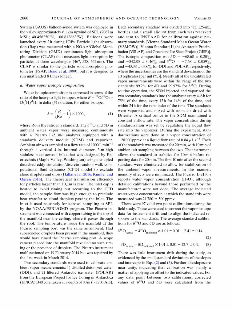
System (GAUS) balloon-sonde system was deployed in
the valley approximately 6.1km upwind of SPL (2067m
MSL; 40.4562508N, 106.8138638W). Balloons were
launched every 2 h during IOPs. Particle light absorp-
tion (Bap) was measured with a NOAA/Global Moni-
toring Division (GMD) continuous light absorption
photometer (CLAP) that measures light absorption by
particles at three wavelengths (467, 528, 652nm). The
CLAP is similar to the particle soot absorption pho-
tometer (PSAP; Bond et al. 1999), but it is designed to
run unattended 8 times longer.
a. Water vapor isotopic composition
Water isotopic composition is expressed in terms of the
ratio of the heavy to light isotopes, whereR5 18O/16O or
D(2H)/1H. In delta (d) notation, for either isotope,
d5
�R
Ro2 1
�3 1000, (1)
where Ro is the ratio in a standard. The d18O and dD in
ambient water vapor were measured continuously
with a Picarro L-2130-i analyzer equipped with a
standards delivery module (SDM) and vaporizer.
Ambient air was sampled at a flow rate of 1000Lmin21
through a vertical 4-in. internal diameter, 3-m-high
stainless steel aerosol inlet that was designed by En-
ertechnix (Maple Valley, Washington) using a coupled
detached eddy simulation/discrete random walk com-
putational fluid dynamics (CFD) model to exclude
cloud droplets and snow (Hallar et al. 2016; Kumler and
Ogren 2016). The theoretical transmission efficiency
for particles larger than 10mm is zero. The inlet cap is
heated to avoid riming but according to the CFD
model, the sample flow was high enough to preclude
heat transfer to cloud droplets passing the inlet. The
inlet is used routinely for aerosol sampling at SPL
by the NOAA/ESRL/GMD program. The Picarro in-
strument was connected with copper tubing to the top of
the manifold near the ceiling, where it passes through
the roof. The temperature inside the manifold at the
Picarro sampling port was the same as ambient. Had
supercooled droplets been present in the manifold, they
would have rimed the Picarro sampling port. A scope
camera placed into the manifold revealed no such rim-
ing or the presence of droplets. The Picarro instrument
malfunctioned on 19 February 2014 but was repaired by
the first week in March 2014.
Two secondary standards were used to calibrate am-
bient vapor measurements: 1) distilled deionized water
(DDI); and 2) filtered Antarctic ice water (POLAR)
from the European Project for Ice Coring in Antarctica
(EPICA) B40 core taken at a depth of 80m (;1200 AD).
Each secondary standard was divided into ten 125-mL
bottles and a small aliquot from each was reserved
and sent to INSTAAR for calibration against pri-
mary standards [Vienna Standard Mean Ocean Water
(VSMOW)], Vienna Standard Light Antarctic Precip-
itation (VSLAP), andGreenland Ice Sheet Project (GISP)].
The isotopic composition was dD 5 268.68 6 0.20&and 2342.80 6 0.46& and d18O 5 27.68 6 0.059&and243.386 0.06& for DDI and POLAR, respectively,
where the uncertainties are the standard deviations of the
10 replicates [per mil (&)]. Nearly all of the uncalibrated
vapor measurements were within the range of the two
standards: 99.2% for dD and 99.97% for d18O. During
routine operation, the SDM injected and vaporized the
two secondary standards into the analyzer every 4–6h for
75% of the time, every 12h for 14% of the time, and
within 24h for the remainder of the time. The standards
were vaporized and mixed with room air dried with
Drierite. A critical orifice in the SDM maintained a
constant airflow rate. The vapor concentration during
standardization was set by regulating the liquid flow
rate into the vaporizer. During the experiment, stan-
dardizations were done at a vapor concentration of
;20 000 ppmv at a liquid flow rate of 0.04 mL s21. Each
of the standards wasmeasured for 20min, with 10min of
ambient air sampling between the two. The instrument
allows the standard to stabilize for 10min before re-
porting data for 20min. The first 10min after the second
standard were eliminated to allow for stabilization of
the ambient vapor measurements. In this manner,
memory effects were minimized. The Picarro L-2130-i
reports water vapor concentration (H2O), although
detailed calibrations beyond those performed by the
manufacturer were not done. The average indicated
water vapor concentration at which the standards were
measured was 21 780 6 500 ppmv.
There were 97 valid two-point calibrations during the
field study. These were used to correct the vapor isotope
data for instrument drift and to align the indicated re-
sponse to the standards. The average standard calibra-
tions for d18O and dD are as follows:
d18OActual
5 d18OIndicated
3 1:016 0:012 2:416 0:14,
(2)
dDActual
5 dDIndicated
3 1:016 0:011 12:7 6 0:9. (3)
There was little instrument drift during the study, as
evidenced by the small standard deviations of the slopes
and intercepts in Eqs. (2) and (3). Further, the slopes are
near unity, indicating that calibration was mainly a
matter of applying an offset to the indicated values. For
any data point between two calibrations, corrected
values of d18O and dD were calculated from the
2666 JOURNAL OF ATMOSPHER IC AND OCEAN IC TECHNOLOGY VOLUME 33

respective end-member equations. A weighted average
of the corrected values of d18O and dD was then calcu-
lated, where the weighting was the ratio of the time
between the data point and the end of the first calibra-
tion to the time between the end of the first calibration
and the beginning of the second calibration.
The uncertainties of the vapor isotopic measurements
have two components: accuracy and precision (re-
peatability of the measurement of a constant attribute).
Accuracy, or bias, is the difference between the true
(VSMOW, VSLAP, and GISP) and unknown values,
which in this case is the secondary standards (POLAR
andDDI). INSTAAR reported upper limits on accuracy
of 0.09& for d18O and 0.78& for dD. There is no error
to minimize for a two-point calibration line. However,
the calibration precision is a function of variability of the
secondary standards (s2Std), as determined by INSTAAR,
and the variability of the measured values of the stan-
dards over the calibration period (s2Meas). The un-
certainties of the slope and intercept of the calibration
line can be obtained by propagating s2Std and s2
Meas
through the calculation using the effective variance ap-
proach [Eq. (2) in Lowenthal et al. 1987]. The contribu-
tions of the calibration process to ambient vapor
measurement precision were 0.33& and 1.73& for d18O
and dD, respectively.
The response and measurement precision of the
Picarro L-2130-i vary as a function of water vapor
concentration (H2O). Aemisegger et al. (2102) charac-
terized these effects for Picarro analyzers with detailed
laboratory experiments. They found that the response of
the Picarro L-2130-i analyzer was nearly flat for d18O
and dD for H2O between 2500 and 30 000 ppmv. To
address these issues, the POLAR standard was in-
troduced to the analyzer to produce indicated vapor
concentrations from ;600 to ;15 000 ppmv by diluting
the vaporized standard with ultradry air and by varying
the liquid standard flow rate (Bastrikov et al. 2014). This
was done at the end of the field study on 5 and 6 March
2014 at SPL after the instrument had been repaired re-
motely by Picarro. Standard measurements at low vapor
concentration could not be reliably done by only re-
ducing the liquid flow rate below 0.01mL s21. Low vapor
concentrations were obtained by removing the critical
orifice in the SDM and manually regulating the flow of
ultradry airflow into the vaporizer (Bastrikov et al.
2014). In this manner, we were able to obtain eight and
seven data points for d18O and dD, respectively. The
isotopic response with respect to the indicated water
vapor concentration is shown in Fig. 2. The response was
flat above ;4000ppmv, but it deviated nonlinearly be-
low that concentration. The solid lines in Fig. 2 represent
second- and third-order polynomial fits for d18O and dD,
respectively, for the indicated H2O concentration be-
tween 644 and 4203ppmv. One dD measurement at
1747 ppmv (Fig. 2) was not included in the regression. It
is not known why dD was heavier than expected during
this run. It is possible that there were problems with the
vaporization, resulting in fractionation or that themanual
regulation of the ultradry dilution air was not stable.
Isotopic composition was corrected for the response bias
at H2O less than 4203ppmv using these functions. Note
that there were only 9 hourly average H2O concentra-
tions less than 1000ppm and that these occurred during
the clear period of 20–26 January 2014. During IOPs,
there were 13 and 1 hourly average concentrations less
than 3000 and 2000ppmv, respectively.
Figure 2 shows that measurement precision decreased
with decreasing H2O concentration below;4000 ppmv.
Table 1 gives the precision (the standard deviation of
measurements of the standard over an approximately
20-min period at constant H2O) as a function of H2O
concentration for the points in the H2O calibration. The
FIG. 2. Isotopic response of the Picarro L-2130-i (a) d18O and
(b) dD to water vapor concentration. Error bars are the standard
deviations of the isotopic composition at each H2O concentration.
Data points in red were not included in the polynomial
regressions.
DECEMBER 2016 LOWENTHAL ET AL . 2667
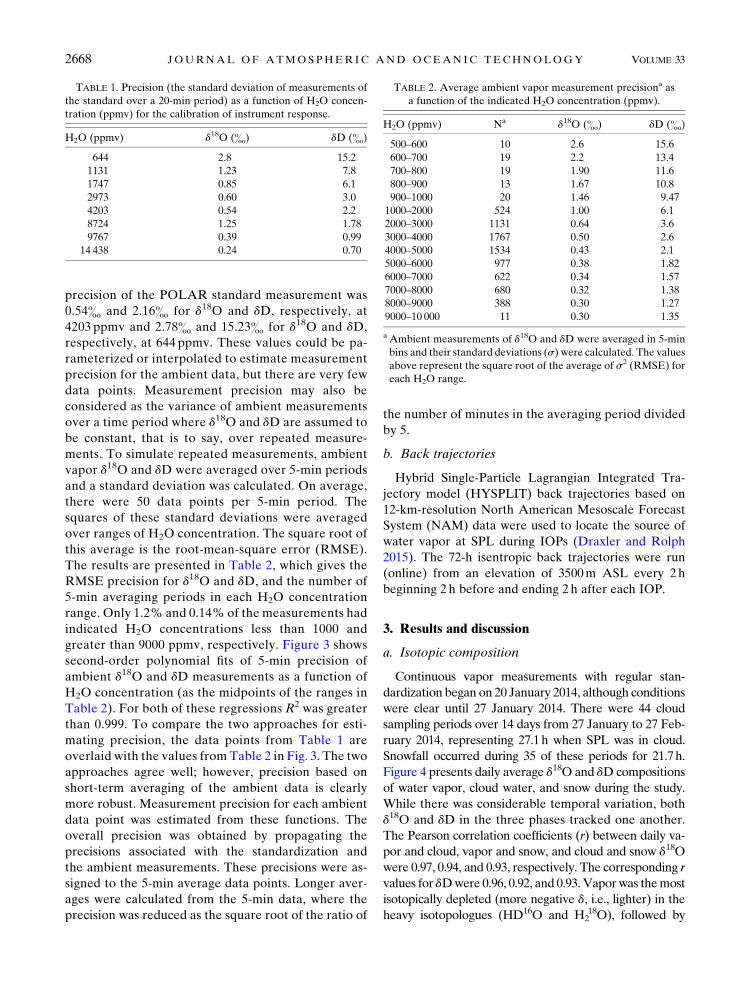
precision of the POLAR standard measurement was
0.54& and 2.16& for d18O and dD, respectively, at
4203 ppmv and 2.78& and 15.23& for d18O and dD,
respectively, at 644 ppmv. These values could be pa-
rameterized or interpolated to estimate measurement
precision for the ambient data, but there are very few
data points. Measurement precision may also be
considered as the variance of ambient measurements
over a time period where d18O and dD are assumed to
be constant, that is to say, over repeated measure-
ments. To simulate repeated measurements, ambient
vapor d18O and dD were averaged over 5-min periods
and a standard deviation was calculated. On average,
there were 50 data points per 5-min period. The
squares of these standard deviations were averaged
over ranges of H2O concentration. The square root of
this average is the root-mean-square error (RMSE).
The results are presented in Table 2, which gives the
RMSE precision for d18O and dD, and the number of
5-min averaging periods in each H2O concentration
range. Only 1.2% and 0.14% of the measurements had
indicated H2O concentrations less than 1000 and
greater than 9000 ppmv, respectively. Figure 3 shows
second-order polynomial fits of 5-min precision of
ambient d18O and dD measurements as a function of
H2O concentration (as the midpoints of the ranges in
Table 2). For both of these regressions R2 was greater
than 0.999. To compare the two approaches for esti-
mating precision, the data points from Table 1 are
overlaid with the values from Table 2 in Fig. 3. The two
approaches agree well; however, precision based on
short-term averaging of the ambient data is clearly
more robust. Measurement precision for each ambient
data point was estimated from these functions. The
overall precision was obtained by propagating the
precisions associated with the standardization and
the ambient measurements. These precisions were as-
signed to the 5-min average data points. Longer aver-
ages were calculated from the 5-min data, where the
precision was reduced as the square root of the ratio of
the number of minutes in the averaging period divided
by 5.
b. Back trajectories
Hybrid Single-Particle Lagrangian Integrated Tra-
jectory model (HYSPLIT) back trajectories based on
12-km-resolution North American Mesoscale Forecast
System (NAM) data were used to locate the source of
water vapor at SPL during IOPs (Draxler and Rolph
2015). The 72-h isentropic back trajectories were run
(online) from an elevation of 3500m ASL every 2h
beginning 2 h before and ending 2 h after each IOP.
3. Results and discussion
a. Isotopic composition
Continuous vapor measurements with regular stan-
dardization began on 20 January 2014, although conditions
were clear until 27 January 2014. There were 44 cloud
sampling periods over 14 days from 27 January to 27 Feb-
ruary 2014, representing 27.1h when SPL was in cloud.
Snowfall occurred during 35 of these periods for 21.7h.
Figure 4 presents daily average d18O and dD compositions
of water vapor, cloud water, and snow during the study.
While there was considerable temporal variation, both
d18O and dD in the three phases tracked one another.
The Pearson correlation coefficients (r) between daily va-
por and cloud, vapor and snow, and cloud and snow d18O
were 0.97, 0.94, and 0.93, respectively. The corresponding r
values for dDwere 0.96, 0.92, and 0.93. Vaporwas themost
isotopically depleted (more negative d, i.e., lighter) in the
heavy isotopologues (HD16O and H218O), followed by
TABLE 2. Average ambient vapor measurement precisiona as
a function of the indicated H2O concentration (ppmv).
H2O (ppmv) Na d18O (&) dD (&)
500–600 10 2.6 15.6
600–700 19 2.2 13.4
700–800 19 1.90 11.6
800–900 13 1.67 10.8
900–1000 20 1.46 9.47
1000–2000 524 1.00 6.1
2000–3000 1131 0.64 3.6
3000–4000 1767 0.50 2.6
4000–5000 1534 0.43 2.1
5000–6000 977 0.38 1.82
6000–7000 622 0.34 1.57
7000–8000 680 0.32 1.38
8000–9000 388 0.30 1.27
9000–10 000 11 0.30 1.35
a Ambient measurements of d18O and dD were averaged in 5-min
bins and their standard deviations (s) were calculated. The values
above represent the square root of the average of s2 (RMSE) for
each H2O range.
TABLE 1. Precision (the standard deviation of measurements of
the standard over a 20-min period) as a function of H2O concen-
tration (ppmv) for the calibration of instrument response.
H2O (ppmv) d18O (&) dD (&)
644 2.8 15.2
1131 1.23 7.8
1747 0.85 6.1
2973 0.60 3.0
4203 0.54 2.2
8724 1.25 1.78
9767 0.39 0.99
14 438 0.24 0.70
2668 JOURNAL OF ATMOSPHER IC AND OCEAN IC TECHNOLOGY VOLUME 33

snow, and then cloud. Daily average differences between
vapor and cloud d18O and between vapor and snow d18O
were 12.1 6 0.8& and 10.9 6 1.3&, respectively. The
corresponding differences for dD were 98.2 6 7.0& and
89.76 12.0&, respectively. The d18O and dD were highly
correlated during vapor (r 5 1.00), cloud (r 5 1.00), and
snow (r 5 0.99) sample periods. Figure 5 presents the re-
lationships between d18O and dD in cloud, snow, and
vapor samples during IOPs. The regressions shown in
Fig. 5 are close to the global meteoric water line (GMWL)
(dD5 8 d18O1 10) foundbyCraig (1961) in naturalwaters
and precipitation, although the intercept for vapor is lower.
The temporal variation of vapor d18O and dD reflects
the history of precipitation (i.e., the fraction of vapor
removed) and any processes that introduce vapor to
the air mass en route to SPL. Daily average vapor d18O
during IOPs varied from 236.0& to 223.8&. Based
on equilibrium fractionation coefficients presented
in Clark and Fritz (1997) from Majoube (1971), a
VSMOW-derived source vapor d18O at 100% RH would
vary by only 1.73& for sea surface temperatures between
308C and 108C. As vapor moves inland, it becomes more
and more isotopically depleted after successive pre-
cipitation events (Dansgaard 1964). Since the saturation
vapor pressure is lower at lower temperatures, the final
vapor d18O and dD at SPL are determined by the tem-
perature gradient between the vapor source and SPL
(Dansgaard 1964; Harmon 1979). This gradient is en-
hanced by orographic lifting (Siegenthaler and Oeschger
1980). Dansgaard (1964) demonstrated that d18O in pre-
cipitation decreased linearlywith decreasingmean annual
air temperature with a slope of 0.7& 8C21 at 38 coastal
stations in the North Atlantic and Greenland, and that
this decreasewas theoretically consistent with the isotopic
lightening of an air mass as it cools during transport from
the oceanic vapor source. Isotopic fractionation during
successive events of vapor condensation under equilib-
rium conditions followed by removal of the condensate is
known as Rayleigh distillation. Similar relationships were
found by Picciotto et al. (1960), Warburton and DeFelice
(1986), and Lowenthal et al. (2011).
The expected isotopic lightening following removal of
water from air masses was demonstrated in coastal
Iceland (Steen-Larsen et al. 2015) and on the eastern
slope of the Colorado Rockies (Noone et al. 2013). This
was also the case during IFRACS. Figure 6 presents a
time series and scatterplot of daily average water vapor
concentration (H2O) and d18O. The relationship was
direct with a moderate correlation (r5 0.62), suggesting
different airmass histories from day to day. However,
Fig. 6 illustrates the effect of Rayleigh distillation up-
wind of SPL, whether or not there was cloud at SPL.
While the isotopic composition of cloud water and snow
at SPL varied from day to day, the differences between
phases was relatively constant. This is consistent with
Rayleigh distillation of the vapor with equilibrium
fractionation en route to SPL.
FIG. 4. Variation of daily average water vapor, cloud, and snow
oxygen isotopic composition (d18O and dD).
FIG. 3. Precision (standard deviation) of 5-min ambient
measurements of (a) d18O and (b) dD as a function of water vapor
(H2O) concentration (open circles). Precision based on the cali-
bration of isotopic composition vs H2O concentration taken from
Table 1 (closed circles).
DECEMBER 2016 LOWENTHAL ET AL . 2669

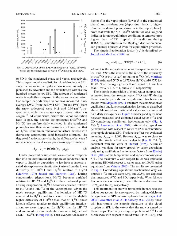
b. Altitude of snow growth
Themass-weighted altitude (MWA) of snowgrowth by
vapor deposition and riming may be inferred from the
relationship between isotopic composition and tempera-
ture (Picciotto et al. 1960; Warburton and DeFelice 1986;
Lowenthal et al. 2011). Based on d18O in precipitation
and surface temperature at 38 coastal North Atlantic and
Greenland sites, Dansgaard (1964, p. 443) concluded: ‘‘If
the mean surface temperature [T] is supposed to vary
parallel to the mean condensation temperature from one
place to another,’’ then dd18O/dT ’ 0.7& 8C21. When
snow ismore depleted than cloud droplets at SPL (Fig. 4),
it follows that it formed aloft at a temperature colder than
that at SPL. This temperature can be estimated as the
difference (D) between d18O in cloud and snow divided
by 0.7. To convert temperature aloft to altitude above
SPL,D ismultiplied by the average of the inverse ambient
lapse rate derived from sounding data within 2km above
SPL during IOPs. This value was relatively stable over
the experiment (1586 20m 8C21). Figure 7 presents daily
MWA, which ranged from just below SPL (253m) to
922m above SPL. On 14 and 16 February, negative
heights could represent growth of ice crystals from iso-
topically enriched vapor or drops in the upslope flow
below SPL.Also plotted in Fig. 7 are the daily differences
(D) between cloud and snow d18O. The seeder–feeder
model (Reinking et al. 2000) suggests that ice nucleation
occurs at a higher altitude than the liquid cloud, which,
based on the soundings, extended from 1 to 2.5km above
SPL on 10 of 14 sampling days. While ice nucleation may
occur above this level, most of the ice mass and its iso-
topic signature accrue much closer to the surface.
c. Isotopic fractionation
The isotopic composition of the vapor phase (V) and
the condensed phase (C) for cloud droplet and ice
crystal growth by vapor deposition is described as
aC2V
aK5 (d
C1 1000)/(d
V1 1000), (4)
where aC2V is the equilibrium fractionation factor, aK is
the kinetic fractionation factor, and dC and dV are d18O
FIG. 6. The relationship between daily water vapor concentra-
tion (H2O) and vapor d18O: (a) time series, also indicating days
on which cloud and snow sampling (IOPs) occurred; and
(b) scatterplot for days without (clear, black circle) and with cloud
and snow (IOPs, red circle) sampling (r 5 Pearson correlation).
FIG. 5. Relationship between d18O and dD in cloud, snow, and
vapor samples. Solid line is the global meteoric water line of Craig
(1961): dD 5 8 d18O 1 10.
2670 JOURNAL OF ATMOSPHER IC AND OCEAN IC TECHNOLOGY VOLUME 33
or dD in the condensed phase and vapor, respectively.
This simple model is realistic for cloud droplets at SPL,
since the vapor in the upslope flow is continuously re-
plenished by advection and the cloud base is within a few
hundred meters below SPL. The amount of condensed
water is negligible compared to the vapor concentration.
For sample periods when vapor was measured, daily
average LWC (from the DMT SPP-100) and IWC (from
the snow collectors) were 0.11 and 0.09 gm23, re-
spectively, while the average vapor concentration was
4.6 gm23. At equilibrium, where the vapor saturation
ratio is one, the heavier isotopologues (HD16O and
H218O) are preferentially enriched in the condensed
phases because their vapor pressures are lower than that
of H216O. Equilibrium fractionation factors increase with
decreasing temperature (and increasing altitude). The
degree of fractionation—that is, the difference between d
in the condensed and vapor phases—is approximately
dC2 d
V’ 1000 ln(a
C2VaK) . (5)
Under nonequilibrium conditions—that is, evapora-
tion into an unsaturated atmosphere or condensation of
vapor to liquid or deposition to ice from a supersatu-
rated atmosphere—a kinetic effect arises from the lower
diffusivity of HD16O and H218O relative to H2
16O
(Merlivat 1978; Jouzel and Merlivat 1984). During
condensation (deposition), H216O becomes enriched
relative to HD16O and H218O in the condensed phase.
During evaporation, H216O becomes enriched relative
to H218O and HD16O in the vapor phase. Given the
much stronger equilibrium fractionation of HD16O
compared to H218O, and to a lesser extent the slightly
higher diffusivity of HD16O than that of H218O, these
kinetic effects, relative to their equilibrium fraction-
ation, are more important for H218O than for HD16O
and are manifested in the deuterium excess (d), defined
as dD2 8 d18O (Craig 1961). Thus, evaporation leads to
higher d in the vapor phase (lower d in the condensed
phase) and condensation (deposition) leads to higher
d in the condensed phase (lower d in the vapor phase).
Note that while the dD2 8 d18O definition of d is a good
indicator for nonequilibrium conditions at temperatures
higher than 2208C (typical of conditions during
IFRACS), curvatures in the Rayleigh distillation curve
can generate nonzero d even for equilibrium processes.
The kinetic fractionation factor (aK) is described by
Jouzel and Merlivat (1984) as
aK5 S/[a
V2CD/D0(S2 1)1 1], (6)
where S is the saturation ratio with respect to water or
ice, andD/D0 is the inverse of the ratio of the diffusivity
of HD16O or H218O (D0) to that of H2
16O (D). Merlivat
(1978) estimatedD0/D as 0.9723 forH218O and 0.9755 for
HDO. Note that aK is greater than 1, equal to 1, and less
than 1 for S , 1, S 5 1, and S . 1, respectively.
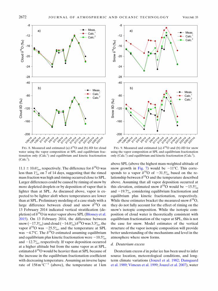
The isotopic composition of cloud water samples was
estimated from the average vapor d18O and dD during
those sample periods and equilibrium fractionation
factors fromMajoube (1971), and from the combination of
equilibrium and kinetic fractionation factors, as described
above. Measured and estimated values were compared
on a daily average basis. Figure 8 shows good agreement
between measured and estimated cloud water d18O and
dD considering equilibrium fractionation only (Fig. 8,
Calc.1). Lowenthal et al. (2002) estimated a typical su-
persaturation with respect to water of 0.5% in wintertime
orographic clouds at SPL. The kinetic effect was evaluated
assuming Swater 5 1.005. Because Swater was so close to
unity, the kinetic effect was negligible (Fig. 8, Calc.2),
consistent with the work of Stewart (1975). A similar
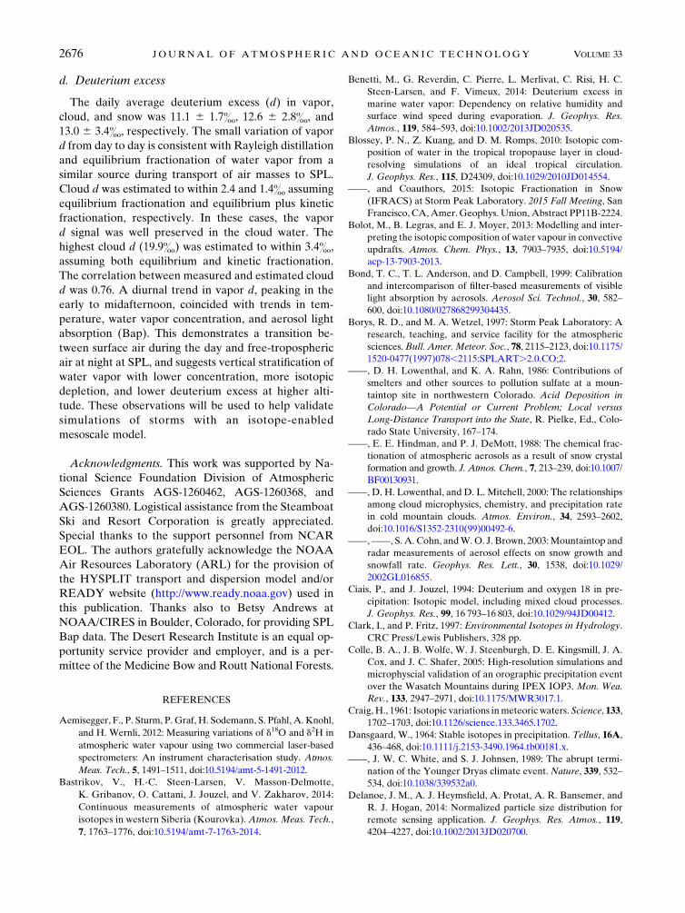
analysis was done for snow growth by vapor deposition
only using equilibrium fractionation factors from Ellehoj
et al. (2013) at the temperature and vapor composition at
SPL. The maximum S with respect to ice was estimated
assuming RH with respect to water equal to 100.5% using
equations from Vaisala (2013). The results are presented
in Fig. 9. Considering equilibrium fractionation only, es-
timated d18O and dD were 4.6& and 29.5& less depleted
than measured d18O and dD, respectively. When kinetic
fractionation was included, these differences decreased to
0.97& and 16.1&, respectively.
This treatment for snow is unrealistic in part because
it does not account for snow growth by riming, which can
be significant at SPL in mixed-phase clouds (Borys et al.
2003; Lowenthal et al. 2011; Saleeby et al. 2013). Snow
will incorporate the isotopic signature of the cloud
droplets at SPL to the extent that the snow is rimed by
those drops. The daily average depletions of d18O and
dD in snow with respect to cloud were 1.446 1.33& and
FIG. 7. Daily MWA above SPL of snow growth (bars). The solid
circles are the differences between d18O in cloud and snow.
DECEMBER 2016 LOWENTHAL ET AL . 2671
11.16 10.6&, respectively. The difference for d18O was
less than 1& on 7 of 14 days, suggesting that the rimed
mass fractionwas high and riming occurred close to SPL.
Larger differences could be caused by riming of snow by
more depleted droplets or by deposition of vapor that is
lighter than at SPL. As discussed above, vapor is ex-
pected to be lighter aloft where temperatures are lower
than at SPL. Preliminary modeling of a case study with a
large difference between cloud and snow d18O on
13 February 2014 indicated vertical stratification (de-
pletion) of d18O in water vapor above SPL (Blossey et al.
2015). On 13 February 2014, the difference between
snow (217.3&) and cloud (214.0&) d18Owas 3.3&, the
vapor d18O was 225.5&, and the temperature at SPL
was 24.78C. The d18O estimated assuming equilibrium
and equilibrium plus kinetic fractionation were210.5&and 212.7&, respectively. If vapor deposition occurred
at a higher altitude but from the same vapor as at SPL,
estimated d18O would be heavier than at SPL because of
the increase in the equilibrium fractionation coefficient
with decreasing temperature. Assuming an inverse lapse
rate of 158m 8C21 (above), the temperature at 1 km
above SPL (above the highest mass-weighted altitude of
snow growth in Fig. 7) would be 2118C. This corre-
sponds to a vapor d18O of 231.5& based on the re-
lationship between d18O and the temperature described
above. Assuming that all vapor deposition occurred at
this elevation, estimated snow d18O would be 215.5&and 219.7& considering equilibrium fractionation and
equilibrium plus kinetic fractionation, respectively.
While these estimates bracket the measured snow d18O,
they do not fully account for the effect of riming on the
snow’s isotopic composition. While the isotopic com-
position of cloud water is theoretically consistent with
equilibrium fractionation of the vapor at SPL, this is not
the case for snow. Model estimates of the vertical
structure of the vapor isotopic composition will provide
better understanding of the mechanisms and level in the
atmosphere where snow forms.
d. Deuterium excess
Deuterium excess d in polar ice has been used to infer
source location, meteorological conditions, and long-
term climate variations (Jouzel et al. 1982; Dansgaard
et al. 1989; Vimeux et al. 1999; Jouzel et al. 2007), water
FIG. 9. Measured and estimated (a) d18O and (b) dD for snow
using the vapor composition at SPL and equilibrium fractionation
only (Calc.1) and equilibrium and kinetic fractionation (Calc.2).
FIG. 8. Measured and estimated (a) d18O and (b) dD for cloud
water using the vapor composition at SPL and equilibrium frac-
tionation only (Calc.1) and equilibrium and kinetic fractionation
(Calc.2).
2672 JOURNAL OF ATMOSPHER IC AND OCEAN IC TECHNOLOGY VOLUME 33

vapor circulation and atmospheric mixing (Blossey et al.
2010), and cloud processes (Bolot et al. 2013; Ciais and
Jouzel 1994; Samuels-Crow et al. 2014). Benetti et al.
(2014) concluded that d was inversely related to RH
above the sea surface and that it increased significantly
as a function of increasing surface roughness, which is a
function of wind speed. Pfahl and Sodemann (2014)
concluded that d varied with RH but not sea surface
temperature (SST). Steen-Larsen et al. (2014) found a
relationship between d and RH on Bermuda, but the
effect of wind speed on d was ambiguous. Steen-Larsen
et al. (2015) concluded that neither wind speed nor SST
had an effect on d in Iceland. The global meteoric water
line of Craig (1961) is consistent with a d of 10& in water
vapor over an oceanic source at RH;85% (Clark and
Fritz 1997).
The temporal variations of daily average vapor, cloud,
and snow d during IOPs are shown in Fig. 10a. Average
vapor, cloud, and snow dwere 11.16 1.7&, 12.66 2.8&,
and 13.0 6 3.4&, respectively. On a daily basis, vapor
d at SPL was roughly consistent with oceanic source
vapor evaporated at 85% RH (Clark and Fritz 1997).
This was also the case for cloud and snow d, although
there were higher values prior to 9 February 2014.
Figure 10a indicates the direction of the source area with
respect to SPL derived from ensemble HYSPLIT back
trajectories during IOPs on each day. All 72-h trajec-
tories ended in the Pacific Ocean except for several on
29 February 2014, which ended in Nevada and Cal-
ifornia. For the 12 days with vapor measurements, the
source directions were west, northwest, and west–
southwest on 8, 3, and 1 days, respectively. Deuterium
excess during IOPs was estimated for cloud (Fig. 10b)
and snow (Fig. 10c) from the estimated d18O and dD,
shown in Figs. 8 and 9, respectively. Cloud d after
6 February 2014 was estimated to within 1.3& and 0.3&,
on average, based on equilibrium and equilibrium plus
kinetic fractionation, respectively. Cloud d was under-
estimated on 27 January, and 4 and 6 February 2014.
As was the case for d18O and dD (Fig. 9), snow d could
not be reproduced assuming growth by vapor deposi-
tion under equilibrium or equilibrium plus kinetic
fractionation.
Welp et al. (2012) reported diurnal cycles of d in
surface water vapor during summer at six urban, agri-
cultural, and rural sites in the United States, Canada,
and China. Deuterium excess increased from noon to
midafternoon at all sites, with amplitudes ranging from
3.5& to 17&. This was attributed to entrainment of
upper-level air as the mixed layer deepened and/or
evapotranspiration from plants.
The diurnal variation of water vapor d during
IFRACS was examined using grand hourly averages for
all hours from 20 January to 19 February 2014. The av-
erage hourly vapor d was 8.96 3.8&. The diurnal cycles
of d, temperature, water vapor concentration (H2O),
and the particle light absorption coefficient at 528 nm
(Bap), an indicator of surface pollution, are shown in
Fig. 11a. Peaks in Bap occurred from 2300 to 0100
mountain standard time (MST). These peaks were
probably caused by snow grooming operations that oc-
curred late at night and into the early morning. After
eliminating the highest 1% of the data (i.e., statistical
outliers), these peaks disappeared. The uncertainties of
d were propagated from those of d18O and dD. The
correlations r between temperature and H2O and be-
tween H2O and d were 0.74 and 0.71, respectively.
Maxima and minima in d, temperature, H2O, and Bap
FIG. 10. (a) Variation of daily d in vapor, cloud, and snow during
IOP sample periods; comparison of measured and calculated d in
(b) cloud and (c) snow. Calc.1 and Calc.2 are as in Figs. 9 and 10.
Wind directions from ensemble HYSPLIT trajectories on each day
are shown in Fig. 10a (W stands for west, NW is for northwest,
WSW is for west-southwest).
DECEMBER 2016 LOWENTHAL ET AL . 2673

occurred during the afternoon (1300–1700 MST) and
early morning (0400–0900 MST), respectively. Average
afternoon and morning d and H2O were 10.3 6 0.4&and 4600 6 140 ppmv and 7.7 6 0.4& and 4200 6140 ppmv, respectively. Thus, the diurnal ranges of d and
H2O were only 2.5& and 400 ppmv. Note that based on
the relationship shown in Fig. 6b, the diurnal variation in
water vapor concentration (400 ppmv) corresponds to a
change in vapor d18O of only 0.49&. Water vapor con-
centration varies by 40% on a daily basis but only by
11%over the diurnal cycle. Figure 11b shows the diurnal
variation of d18O and dD. There was no clear diurnal
trend for d18O and dD (consistent with the small
diurnal variation of water vapor concentration), al-
though their divergence between 1300 and approxi-
mately 2000 MST is responsible for the afternoon peak
in vapor d. The small variation of water vapor concentra-
tion and its isotopic composition at night supports the
suggestion in section 3a (Fig. 6b) that their daily variation
is related to Rayleigh distillation during transport to SPL.
SPL is above the surface inversion overnight and into
the morning hours. Lower temperature and Bap during
that period represent background or free-tropospheric
air (Borys et al. 1986; Lowenthal et al. 2002; Obrist et al.
2008). During the daytime, surface-derived aerosols (as
indicated by Bap) are mixed up to the level of SPL. As
discussed above, kinetic fractionation during conden-
sation increased estimated d in the condensate—for
example, cloud (Fig. 10b) and snow (Fig. 10c)—
although the effect is much greater for snow. The effect
is opposite for d in the vapor. Figure 12 shows aweak but
direct relationship between daily average H2O concen-
tration and vapor d at SPL. This is expected if the
fraction ( f) of water vapor remaining after transport to
SPL is proportional to the vapor concentration at SPL
and if kinetic fractionation occurred during condensa-
tion and precipitation upwind of SPL. This mechanism,
which is seen on a day-to-day basis, is consistent with the
diurnal variation in H2O and vapor d. The diurnal var-
iation in d suggests vertical stratification of water vapor,
FIG. 11. Diurnal variation of (a) deuterium excess d, temperature, water vapor (H2O), and
Bap for the bottom 99% of the data; and (b) diurnal variation of d18O and dD.
2674 JOURNAL OF ATMOSPHER IC AND OCEAN IC TECHNOLOGY VOLUME 33

which becomes drier and more isotopically depleted
with a lower d with increasing altitude. Another pro-
cess that could elevate d during the daytime is evapo-
ration from upwind surface snow. Kinetic fractionation
could occur if there was melting followed by evapora-
tion at the snow surface. This is certainly possible as
even under cloudy conditions at SPL during IOPs, the
average surface temperature and RH at the GAUS
launch site were 1.38C and 73%, respectively. Rela-
tively small day-to-day variation of d in vapor, cloud
water, and snow suggests a relatively constant vapor
source. However, the diurnal variation of d demon-
strates the influence of colder, drier free-tropospheric air
with lower d during the nighttime and early morning
hours in contrast with higher d in moister surface air
during the afternoon hours.
4. Conclusions
Water isotopologues (HD16O and H218O) were
measured in water vapor, supercooled cloud droplets,
and falling snow in mixed-phase wintertime orgo-
graphic clouds at Storm Peak Laboratory (SPL, 3210m
MSL) from 20 January to 27 February 2014 during the
Isotopic Fractionation in Snow (IFRACS) study. A
Picarro L-2130-i analyzer continuously measured d18O
and dD in atmospheric water vapor until 19 February.
Cloud and snow were sampled when SPL was envel-
oped in snowing cloud in discrete intervals totaling
21.7 h over 14 days.
a. Isotopic composition
Water vapor was the most isotopically depleted, fol-
lowed by snow, and then cloud. The d18O and dD were
nearly perfectly correlated (r. 0.99) in all three phases
and closely followed the global meteoric water line of
Craig (1961). There were strong correlations between
daily d18O in vapor and cloud (r5 0.97), vapor and snow
(r 5 0.94), and cloud and snow (r 5 0.93). The differ-
ences between vapor and cloud and between vapor and
snow d18O were similar from day to day, consistent with
Rayleigh distillation and equilibrium fractionation dur-
ing transport to SPL. This also suggests relatively con-
sistent cloud condensation and snow growth processes
during the experiment.
b. Altitude of snow growth
The altitude at which the snow accrued most of its
mass was inferred from relationships between cloud and
snow d18O, a literature-based dd18O/dT of 0.7& 8C21,
and a consistent ambient lapse rate over the course of
the field study. The estimated mass-weighted altitude of
snow growth was within 1km of SPL on all days and
within 500m of SPL on 9 out of 14 study days. These
results are similar to those found in a previous study at
SPL (Lowenthal et al. 2011). While ice crystals may
nucleate under subsaturated conditions higher in the
atmosphere, they gain most of their ice mass by vapor
deposition and riming at much lower levels in the
orographic cloud.
c. Isotopic fractionation
The isotopic composition of cloud water at SPL was
closely reproduced from the vapor composition at SPL
and literature-based equilibrium fractionation factors.
Estimated d18O decreased by only 0.2&, on average, if
the potential effects of kinetic fractionation were con-
sidered. Estimating the isotopic composition of snow
was more difficult. Assuming depositional growth only,
the vapor composition observed at SPL, and equilibrium
fractionation, the estimated snow composition was sig-
nificantly heavier than that observed. Adding kinetic
fractionation increased the estimated depletion; how-
ever, this treatment is unrealistic in part because snow
growth occurs by riming as well as by vapor deposition.
The difference between cloud and snow d18O was less
than 1& on 7 of 14 days, suggesting that snow on these
days gainedmuch of its mass and isotopic signature from
riming close to SPL. Thus, near-surface riming can
have a significant effect on the isotopic composition of
deposited snow. For larger differences between cloud
and snow d18O, growth likely occurred by deposition of
vapor that was isotopically lighter than that observed at
SPL or by riming of droplets derived from that vapor.
This implies that the vapor and its isotopic composition
were vertically stratified. Vapor depletion with in-
creasing altitude is consistent with previous observa-
tions and our understanding of isotopic fractionation
as a function of temperature.
FIG. 12. Relationship between daily average water vapor concen-
tration (H2O) and vapor d.
DECEMBER 2016 LOWENTHAL ET AL . 2675
d. Deuterium excess
The daily average deuterium excess (d) in vapor,
cloud, and snow was 11.1 6 1.7&, 12.6 6 2.8&, and
13.0 6 3.4&, respectively. The small variation of vapor
d from day to day is consistent with Rayleigh distillation
and equilibrium fractionation of water vapor from a
similar source during transport of air masses to SPL.
Cloud d was estimated to within 2.4 and 1.4& assuming
equilibrium fractionation and equilibrium plus kinetic
fractionation, respectively. In these cases, the vapor
d signal was well preserved in the cloud water. The
highest cloud d (19.9&) was estimated to within 3.4&,
assuming both equilibrium and kinetic fractionation.
The correlation between measured and estimated cloud
d was 0.76. A diurnal trend in vapor d, peaking in the
early to midafternoon, coincided with trends in tem-
perature, water vapor concentration, and aerosol light
absorption (Bap). This demonstrates a transition be-
tween surface air during the day and free-tropospheric
air at night at SPL, and suggests vertical stratification of
water vapor with lower concentration, more isotopic
depletion, and lower deuterium excess at higher alti-
tude. These observations will be used to help validate
simulations of storms with an isotope-enabled
mesoscale model.
Acknowledgments. This work was supported by Na-
tional Science Foundation Division of Atmospheric
Sciences Grants AGS-1260462, AGS-1260368, and
AGS-1260380. Logistical assistance from the Steamboat
Ski and Resort Corporation is greatly appreciated.
Special thanks to the support personnel from NCAR
EOL. The authors gratefully acknowledge the NOAA
Air Resources Laboratory (ARL) for the provision of
the HYSPLIT transport and dispersion model and/or
READY website (http://www.ready.noaa.gov) used in
this publication. Thanks also to Betsy Andrews at
NOAA/CIRES in Boulder, Colorado, for providing SPL
Bap data. The Desert Research Institute is an equal op-
portunity service provider and employer, and is a per-
mittee of the Medicine Bow and Routt National Forests.
REFERENCES
Aemisegger, F., P. Sturm, P. Graf, H. Sodemann, S. Pfahl, A. Knohl,
and H. Wernli, 2012: Measuring variations of d18O and d2H in
atmospheric water vapour using two commercial laser-based
spectrometers: An instrument characterisation study. Atmos.
Meas. Tech., 5, 1491–1511, doi:10.5194/amt-5-1491-2012.
Bastrikov, V., H.-C. Steen-Larsen, V. Masson-Delmotte,
K. Gribanov, O. Cattani, J. Jouzel, and V. Zakharov, 2014:
Continuous measurements of atmospheric water vapour
isotopes in western Siberia (Kourovka). Atmos. Meas. Tech.,
7, 1763–1776, doi:10.5194/amt-7-1763-2014.
Benetti, M., G. Reverdin, C. Pierre, L. Merlivat, C. Risi, H. C.
Steen-Larsen, and F. Vimeux, 2014: Deuterium excess in
marine water vapor: Dependency on relative humidity and
surface wind speed during evaporation. J. Geophys. Res.
Atmos., 119, 584–593, doi:10.1002/2013JD020535.
Blossey, P. N., Z. Kuang, and D. M. Romps, 2010: Isotopic com-
position of water in the tropical tropopause layer in cloud-
resolving simulations of an ideal tropical circulation.
J. Geophys. Res., 115, D24309, doi:10.1029/2010JD014554.
——, and Coauthors, 2015: Isotopic Fractionation in Snow
(IFRACS) at Storm Peak Laboratory. 2015 Fall Meeting, San
Francisco, CA,Amer.Geophys.Union,Abstract PP11B-2224.
Bolot, M., B. Legras, and E. J. Moyer, 2013: Modelling and inter-
preting the isotopic composition of water vapour in convective
updrafts. Atmos. Chem. Phys., 13, 7903–7935, doi:10.5194/
acp-13-7903-2013.
Bond, T. C., T. L. Anderson, and D. Campbell, 1999: Calibration
and intercomparison of filter-based measurements of visible
light absorption by aerosols. Aerosol Sci. Technol., 30, 582–
600, doi:10.1080/027868299304435.
Borys, R. D., and M. A. Wetzel, 1997: Storm Peak Laboratory: A
research, teaching, and service facility for the atmospheric
sciences.Bull. Amer. Meteor. Soc., 78, 2115–2123, doi:10.1175/
1520-0477(1997)078,2115:SPLART.2.0.CO;2.
——, D. H. Lowenthal, and K. A. Rahn, 1986: Contributions of
smelters and other sources to pollution sulfate at a moun-
taintop site in northwestern Colorado. Acid Deposition in
Colorado—A Potential or Current Problem; Local versus
Long-Distance Transport into the State, R. Pielke, Ed., Colo-
rado State University, 167–174.
——, E. E. Hindman, and P. J. DeMott, 1988: The chemical frac-
tionation of atmospheric aerosols as a result of snow crystal
formation and growth. J. Atmos. Chem., 7, 213–239, doi:10.1007/
BF00130931.
——, D. H. Lowenthal, and D. L. Mitchell, 2000: The relationships
among cloud microphysics, chemistry, and precipitation rate
in cold mountain clouds. Atmos. Environ., 34, 2593–2602,
doi:10.1016/S1352-2310(99)00492-6.
——,——, S.A. Cohn, andW.O. J. Brown, 2003:Mountaintop and
radar measurements of aerosol effects on snow growth and
snowfall rate. Geophys. Res. Lett., 30, 1538, doi:10.1029/
2002GL016855.
Ciais, P., and J. Jouzel, 1994: Deuterium and oxygen 18 in pre-
cipitation: Isotopic model, including mixed cloud processes.
J. Geophys. Res., 99, 16 793–16 803, doi:10.1029/94JD00412.
Clark, I., and P. Fritz, 1997: Environmental Isotopes in Hydrology.
CRC Press/Lewis Publishers, 328 pp.
Colle, B. A., J. B. Wolfe, W. J. Steenburgh, D. E. Kingsmill, J. A.
Cox, and J. C. Shafer, 2005: High-resolution simulations and
microphyscial validation of an orographic precipitation event
over the Wasatch Mountains during IPEX IOP3. Mon. Wea.
Rev., 133, 2947–2971, doi:10.1175/MWR3017.1.
Craig, H., 1961: Isotopic variations inmeteoric waters. Science, 133,
1702–1703, doi:10.1126/science.133.3465.1702.
Dansgaard, W., 1964: Stable isotopes in precipitation. Tellus, 16A,
436–468, doi:10.1111/j.2153-3490.1964.tb00181.x.
——, J. W. C. White, and S. J. Johnsen, 1989: The abrupt termi-
nation of the Younger Dryas climate event. Nature, 339, 532–
534, doi:10.1038/339532a0.
Delanoe, J. M., A. J. Heymsfield, A. Protat, A. R. Bansemer, and
R. J. Hogan, 2014: Normalized particle size distribution for
remote sensing application. J. Geophys. Res. Atmos., 119,
4204–4227, doi:10.1002/2013JD020700.
2676 JOURNAL OF ATMOSPHER IC AND OCEAN IC TECHNOLOGY VOLUME 33
Demoz, B. B., J. A. Warburton, and R. H. Stone, 1991: The influ-
ence of riming on the oxygen isotopic composition of ice-
phase precipitation. Atmos. Res., 26, 463–488, doi:10.1016/
0169-8095(91)90039-Y.
Draxler, R. R., and G. D. Rolph, 2015: HYSPLIT model access.
NOAAAir Resources Laboratory. [Available online at http://
www.arl.noaa.gov/HYSPLIT.php.]
Ellehoj,M.D.,H. C. Steen-Larsen, S. J. Johnsen, andM.B.Madsen,
2013: Ice-vapor equilibrium fractionation factor of hydrogen
and oxygen isotopes: Experimental investigations and impli-
cations for stable water isotope studies. Rapid Commun. Mass
Spectrom., 27, 2149–2158, doi:10.1002/rcm.6668.
Gedzelman, S. D., and J. R. Lawrence, 1990: The isotopic composi-
tion of precipitation from two extratropical cyclones. Mon.
Wea. Rev., 118, 495–509, doi:10.1175/1520-0493(1990)118,0495:
TICOPF.2.0.CO;2.
——, and R. Arnold, 1994: Modeling the isotopic composition of
precipitation. J. Geophys. Res., 99, 10 455–10 471, doi:10.1029/
93JD03518.
Hallar, A. G., I. B. Mccubbin, I. Novosselov, R. Gorder, and
J. Ogren, 2016: A high elevation aerosol manifold modeling
study and inter-comparison. 2012 Fall Meeting, San Francisco,
CA, Amer. Geophys. Union, Abstract A51A-0016.
Harmon, R. S., 1979: An isotopic study of groundwater seepage in
the central Kentucky Karst. Water Resour. Res., 15, 476–480,
doi:10.1029/WR015i002p00476.
Heymsfield, A. J., C. Schmitt, and A. Bansemer, 2013: Ice cloud par-
ticle size distributions and pressure-dependent terminal velocities
from in situ observations at temperatures from 08 to 2868C.J. Atmos. Sci., 70, 4123–4154, doi:10.1175/JAS-D-12-0124.1.
Hindman, E. E., E. J. Carter, R. D. Borys, andD. L.Mitchell, 1992:
Collecting super-cooled droplets as a function of droplet
size. J. Atmos. Oceanic Technol., 9, 337–353, doi:10.1175/
1520-0426(1992)009,0337:CSCDAA.2.0.CO;2.
Hobbs, P. V., 1975: The nature of winter clouds and precipitation in
the Cascade Mountains and their modification by artificial
seeding. Part I: Natural conditions. J. Appl. Meteor., 14, 783–804,
doi:10.1175/1520-0450(1975)014,0783:TNOWCA.2.0.CO;2.
Houze, R. A., and S. Medina, 2005: Turbulence as a mechanism for
orographic precipitation enhancement. J. Atmos. Sci., 62,
3599–3623, doi:10.1175/JAS3555.1.
Joussaume, S., R. Sadourny, and J. Jouzel, 1984: A general circu-
lation model of water isotope cycles in the atmosphere. Na-
ture, 311, 24–29, doi:10.1038/311024a0.
Jouzel, J., and L. Merlivat, 1984: Deuterium and oxygen 18 in
precipitation: Modeling of the isotopic effects during snow
formation. J. Geophys. Res., 89, 11 749–11 757, doi:10.1029/
JD089iD07p11749.
——, ——, and C. Lorius, 1982: Deuterium excess in an East
Antarctic ice core suggests higher relative humidity at the
oceanic surface during the last glacial maximum. Nature, 299,
688–691, doi:10.1038/299688a0.
——, and Coauthors, 2007: The GRIP deuterium-excess record.
Quat. Sci. Rev., 26, 1–17, doi:10.1016/j.quascirev.2006.07.015.
Kumler, A., and J. Ogren, 2016: A comparison of inlet setups at
Storm Peak Laboratory. NOAA, 1 p. [Available online at
http://www.esrl.noaa.gov/gmd/publications/annual_meetings/
2016/abstracts/24-160406-B.pdf.]
Kusunoki, K.,M.Murakami, N.Orikasa,M.Hoshimoto,Y. Tanaka,
H. Mizuno, K. Hamazu, and H. Watanabe, 2005: Observations
of quasi-stationary and shallow orographic snow clouds: Spatial
distributions of supercooled liquid water and snow particles.
Mon. Wea. Rev., 133, 743–751, doi:10.1175/MWR2874.1.
Lamb, D., K. W. Nielsen, H. E. Klieforth, and J. Hallett, 1976:
Measurement of liquidwater content in cloud systems over the
Sierra Nevada. J. Appl. Meteor., 15, 763–775, doi:10.1175/
1520-0450(1976)015,0763:MOLWCI.2.0.CO;2.
Lee, J.-E., R. Pierrehumbert, A. Swann, and B. R. Linter, 2009a:
Sensitivity of stable water isotopic values to convective pa-
rameterization schemes. Geophys. Res. Lett., 36, L23801,
doi:10.1029/2009GL040880.
——, K. Johnson, and I. Fung, 2009b: Precipitation over South
America during the Last Glacial Maximum: An analysis of the
‘‘amount effect’’ with a water isotope-enabled general circu-
lation model. Geophys. Res. Lett., 36, L19701, doi:10.1029/
2009GL039265.
Lorius, C., L. Merlivat, J. Jouzel, and M. Pourchet, 1979: A
30,000 yr isotopic climate record from Antarctic ice. Nature,
280, 644–648, doi:10.1038/280644a0.
Lowenthal, D. H., R. C. Hanumara, K. A. Rahn, and L. A. Currie,
1987: Effects of systematic error, estimates and uncertainties in
chemical mass balance apportionments: Quail Roost II revisited.
Atmos. Environ., 21, 501–510, doi:10.1016/0004-6981(87)90033-3.
——, R. D. Borys, and M. A. Wetzel, 2002: Aerosol distributions
and cloud interactions at a mountaintop laboratory.
J. Geophys. Res., 107, doi:10.1029/2001JD002046.
——,——,W. Cotton, S. Saleeby, S. A. Cohn, andW. O. J. Brown,
2011: The altitude of snow growth by riming and vapor de-
position in mixed-phase orographic clouds. Atmos. Environ.,
45, 519–522, doi:10.1016/j.atmosenv.2010.09.061.
Majoube, M., 1971: Fractionnement en oxygène-18 et en deuté-rium entre l’eau et sa vapeur. J. Chim. Phys., 68, 1423–1436.
Masson-Delmotte, V., and Coauthors, 2008: A review of Antarctic
surface snow isotopic composition: Observations, atmospheric
circulation, and isotopic modeling. J. Climate, 21, 3359–3387,
doi:10.1175/2007JCLI2139.1.
Merlivat, L., 1978:Molecular diffusivities ofH2160,HD160, andH2
180 in
gases. J. Chem. Phys., 69, 2864–2871, doi:10.1063/1.436884.
Moore, M., P. Blossey, A. Muhlbauer, and Z. Kuang, 2016: Mi-
crophysical controls on the isotopic composition of wintertime
orographic precipitation. J. Geophys. Res. Atmos., 121, 7235–
7253, doi:10.1002/2015JD023763.
Muhlbauer, A., T. Hashino, L. Xue, A. Teller, U. Lohmann, R. M.
Rasmussen, I. Geresdi, and Z. Pan, 2010: Intercomparison of
aerosol-cloud-precipitation interactions in stratiform oro-
graphic mixed-phase clouds. Atmos. Chem. Phys., 10, 8173–
8196, doi:10.5194/acp-10-8173-2010.
Noone, D., and I. Simmonds, 2002: Associations between d18O of
water and climate parameters in a simulation of atmospheric
circulation for 1979–95. J. Climate, 15, 3150–3169, doi:10.1175/
1520-0442(2002)015,3150:ABOOWA.2.0.CO;2.
——, and Coauthors, 2013: Determining water sources in
the boundary layer from tall tower profiles of water vapor
and surface water isotope ratios after a snowstorm in
Colorado. Atmos. Chem. Phys., 13, 1607–1623, doi:10.5194/
acp-13-1607-2013.
Obrist, D., A.G.Hallar, I.McCubbin, B. B. Stephens, and T. Rahn,
2008: Atmospheric mercury concentrations at Storm Peak
Laboratory in the Rocky Mountains: Evidence for long-range
transport from Asia, boundary layer contributions, and plant
mercury uptake.Atmos. Environ., 42, 7579–7589, doi:10.1016/
j.atmosenv.2008.06.051.
Pausata, F. S. R., D. S. Battisti, K. H. Nisancioglu, and C. M. Bitz,
2011: Chinese stalagmite controlled by changes in the Indian
monsoon during a simulated Heinrich event. Nat. Geosci., 4,
474–480, doi:10.1038/ngeo1169.
DECEMBER 2016 LOWENTHAL ET AL . 2677

Pfahl, S., and H. Sodemann, 2014: What controls deuterium excess
in global precipitation?Climate Past, 10, 771–781, doi:10.5194/
cp-10-771-2014.
——, H. Wernli, and K. Yoshimura, 2012: The isotopic composi-
tion of precipitation from a winter storm—A case study with
the limited-area model COSMOiso. Atmos. Chem. Phys., 12,
1629–1648, doi:10.5194/acp-12-1629-2012.
Picciotto, E., X. De Maere, and I. Friedman, 1960: Isotopic com-
position and temperature of formation of Antarctic snows.
Nature, 187, 857–859, doi:10.1038/187857a0.
Poage, M. A., and C. P. Chamberlain, 2001: Empirical relationships
between elevation and the stable isotope composition of pre-
cipitation and surface waters: Considerations for studies of paleo-
elevation change. Amer. J. Sci., 301, 1–15, doi:10.2475/ajs.301.1.1.
Rauber, R. M., and L. O. Grant, 1986a: The characteristics and
distribution of cloud water over the mountains of northern
Colorado during wintertime storms. Part II: Microphysical
characteristics. J. Climate Appl. Meteor., 25, 489–504,
doi:10.1175/1520-0450(1986)025,0489:TCADOC.2.0.CO;2.
——, ——, D. Feng, and J. B. Snider, 1986b: The characteristics
and distribution of cloudwater over themountains of northern
Colorado during wintertime storms. Part I: temporal varia-
tions. J. Climate Appl. Meteor., 25, 468–488, doi:10.1175/
1520-0450(1986)025,0468:TCADOC.2.0.CO;2.
Reinking, R. F., J. B. Snider, and J. L. Coen, 2000: Influences of
storm-embedded orographic gravity waves on cloud liquid
water and precipitation. J. Appl. Meteor., 39, 733–759,
doi:10.1175/1520-0450(2000)039,0733:IOSEOG.2.0.CO;2.
Risi, C., S. Bony, F. Vimeux, C. Frankenberg, D. Noone, and
J. Worden, 2010: Understanding the Sahelian water budget
through the isotopic composition of water vapor and pre-
cipitation. J. Geophys. Res., 115, D24110, doi:10.1029/
2010JD014690.
Rotunno, R., and R. A. Houze, 2007: Lessons on orographic pre-
cipitation from the Mesoscale Alpine Programme. Quart.
J. Roy. Meteor. Soc., 133, 811–830, doi:10.1002/qj.67.
Rowley, D. B., R. T. Pierrehumbert, and B. S. Currie, 2001: A new
approach to stable isotope-based paleoaltimetry: Implication
for paleoaltimetry and paleohypsometry of the high Himalaya
since the Late Miocene. Earth Planet. Sci. Lett., 188, 253–268,
doi:10.1016/S0012-821X(01)00324-7.
Saleeby, S. M., W. R. Cotton, D. Lowenthal, J. Messina, and K. B.
Benedict, 2013: Aerosol impacts on the microphysical growth
processes of orographic snowfall. J. Appl. Meteor. Climatol.,
52, 834–852, doi:10.1175/JAMC-D-12-0193.1.
Samuels-Crow, K. E., J. Galewsky, Z. D. Sharp, and K. J. Dennis,
2014: Deuterium excess in subtropical free troposphere water
vapor: Continuous measurements from the Chajnantor Pla-
teau, northern Chile. Geophys. Res. Lett., 41, 8652–8659,
doi:10.1002/2014GL062302.
Schmidt, G. A., G. Hoffmann, D. T. Shindell, and Y. Hu, 2005:
Modeling atmospheric stable water isotopes and the potential
for constraining cloud processes and stratosphere-troposphere
water exchange. J. Geophys. Res., 110, D21314, doi:10.1029/
2005JD005790.
Scholl, M. A., T. W. Giambelluca, S. B. Gingerich, M. A. Nullet,
and L. L. Loope, 2007: Cloud water in windward and leeward
mountain forests: The stable isotope signature of orographic
cloud water. Water Resour. Res., 43, W12411, doi:10.1029/
2007WR006011.
Siegenthaler, U., and H. Oeschger, 1980: Correlation of 18O in
precipitation with temperature and altitude.Nature, 285, 314–
317, doi:10.1038/285314a0.
Smith, J. A., A. S. Ackerman, E. J. Jensen, and O. B. Toon, 2006:
Role of deep convection in establishing the isotopic compo-
sition of water vapor in the tropical transition layer.Geophys.
Res. Lett., 33, L06812, doi:10.1029/2005GL024078.
Smith, R. B., and J. P. Evans, 2007: Orographic precipitation and
water vapor fractionation over the southern Andes.
J. Hydrometeor., 8, 3–19, doi:10.1175/JHM555.1.
——, I. Barstad, and L. Bonneau, 2005: Oregon’s precipitation and
Oregon’s climate transition. J. Atmos. Sci., 62, 177–191,
doi:10.1175/JAS-3376.1.
Steen-Larsen, H. C., and Coauthors, 2011: Understanding the cli-
mate signal in the water stable isotope records from the
NEEM shallow firn/ice cores in northwest Greenland.
J. Geophys. Res., 116, D06108, doi:10.1029/2010JD014311.
——, and Coauthors, 2014: Climatic controls on water vapor deute-
rium excess in the marine boundary layer of the North Atlantic
based on 500 days of in situ, continuous measurements. Atmos.
Chem. Phys., 14, 7741–7756, doi:10.5194/acp-14-7741-2014.
——, and Coauthors, 2015: Moisture sources and synoptic to sea-
sonal variability of North Atlantic water vapor isotopic com-
position. J. Geophys. Res. Atmos., 120, 5757–5774, doi:10.1002/
2015JD023234.
Stewart,M.K., 1975: Stable isotope fractionation due to evaporation
and isotopic exchange of falling waterdrops: Applications to
atmospheric processes and evaporation of lakes. J. Geophys.
Res., 80, 1133–1146, doi:10.1029/JC080i009p01133.Sturm, C., G. Hoffman, and B. Langmann, 2007: Simulation of
stable water isotopes in precipitation over South America:
Comparing regional to global circulation models. J. Climate,
20, 3730–3750, doi:10.1175/JCLI4194.1.Vaisala, 2013: Humidity conversion formulas. Vaisala Oyj Doc.
B210973EN-F, 17 pp. [Available online at http://www.
vaisala.com/Vaisala%20Documents/Application%20notes/
Humidity_Conversion_Formulas_B210973EN-F.pdf.]
Vimeux, F., V. Masson, J. Jouzel, M. Stievenard, and J. R. Petit, 1999:
Glacial–interglacial changes in ocean surface conditions in the
Southern Hemisphere. Nature, 398, 410–413, doi:10.1038/18860.Warburton, J. A., and T. P. DeFelice, 1986: Oxygen isotopic
composition of central Sierra Nevada precipitation, I. Identi-
fication of ice-phase water capture regions in winter storms.
Atmos. Res., 20, 11–22, doi:10.1016/0169-8095(86)90004-9.Welp, L. R., and Coauthors, 2012: A meta-analysis of water vapor
deuterium-excess in the midlatitude atmospheric surface
layer. Global Biogeochem. Cycles, 26, GB3021, doi:10.1029/
2011GB004246.
Werner, M., P. M. Langebroek, T. Carlsen, M. Herold, and
G. Lohmann, 2011: Stable water isotopes in the ECHAM5
general circulation model: Toward a high-resolution isotope
modeling on a global scale. J. Geophys. Res., 116, D15109,
doi:10.1029/2011JD015681.
Wetzel, M., and Coauthors, 2004: Mesoscale snowfall predic-
tion and verification in mountainous terrain. Wea. Forecas-
ting, 19, 806–828, doi:10.1175/1520-0434(2004)019,0806:
MSPAVI.2.0.CO;2.
Wright, J. S., A. H. Sobel, and G. A. Schmidt, 2009: Influence of
condensate evaporation on water vapor and its stable isotopes
in a GCM. Geophys. Res. Lett., 36, L12804, doi:10.1029/
2009GL038091.
Yoshimura, K., C. Frankenberg, J. Lee, M. Kanamitsu, J. Worden,
and T. Röckmann, 2011: Comparison of an isotopic atmo-
spheric general circulation model with new quasi-global sat-
ellitemeasurements of water vapor isotopologues. J. Geophys.
Res., 116, D19118, doi:10.29/2011JD016035.
2678 JOURNAL OF ATMOSPHER IC AND OCEAN IC TECHNOLOGY VOLUME 33