ISIS: A two-scale framework to sparse inference · Example: Economics, Finance, Marketing HPIs /...
69
ISIS: A two-scale framework to sparse inference Jianqing Fan Princeton University http://www.princeton.edu/∼jqfan March 26, 2010 Jianqing Fan (Princeton University) Sparse inference ENAR 1 / 42
Transcript of ISIS: A two-scale framework to sparse inference · Example: Economics, Finance, Marketing HPIs /...

ISIS: A two-scale framework to sparse inference
Jianqing Fan
Princeton University
http://www.princeton.edu/∼jqfan
March 26, 2010
Jianqing Fan (Princeton University) Sparse inference ENAR 1 / 42
Outline
1 Introduction
2 Challenge of Dimensionality
3 The ISIS Method
4 Sparse Survival analysis
5 Numerical Examples
Jianqing Fan (Princeton University) Sparse inference ENAR 2 / 42
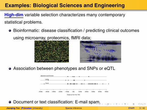
Examples: Biological Sciences and Engineering
High-dim variable selection characterizes many contemporary
statistical problems.
Bioinformatic: disease classification / predicting clinical outcomes
using microarray, proteomics, fMRI data;
Association between phenotypes and SNPs or eQTL
Distance from the TSS
−500kb −400kb −300kb −200kb −100kb 0kb 100kb 200kb 300kb 400kb 500kb
Japanese and Chinese
CEPH
Yorub
Document or text classification: E-mail spam.Jianqing Fan (Princeton University) Sparse inference ENAR 3 / 42

Example: Economics, Finance, Marketing
HPIs / drug sales collected in many regions
Local correlation makes dimensionality growths quickly.Sample Correlation
50 100 150 200 250 300 350
50
100
150
200
250
300
350
PLS Residuals Correlation Cond. on National HPI
50 100 150 200 250 300 350
50
100
150
200
250
300
350
1000 neighborhoods requires 1 m parameters.
Managing 2K stocks involves 2m elements in covariance.
Jianqing Fan (Princeton University) Sparse inference ENAR 4 / 42

Example: Spatial temporal data
�Meteorology & Earth Sciences & Ecology
Temperatures and other attributes (precipitation, population size)
are collected over time and over many regions.
Sheet 1
0.000 1.000
Sum of F(1,1)
Sum of Volumn0
500
1,000
1,500
2,000
2,603
Map based on Longitude (generated) and Latitude (generated). Color show s sum of F(1,1). Size show s sum of Volumn. Details are show n for State and County. 0 5 10 15 20 25
1e+
063e
+06
5e+
067e
+06
Mar
ket S
ale
Large panel data over a short time horizon poses more challenges.
Jianqing Fan (Princeton University) Sparse inference ENAR 5 / 42

Growth of Dimensionality
�Dimen. grows rapidly w/ interactions: 5000 12.5m.
Synergy of Two Genes: colon cancer in Hanczar et al (2007).
e.g., Y = I(X1 +X2 > 3) and Y ⊥ X1.
G1
50% 50%
0%
white – patients; black – normalJianqing Fan (Princeton University) Sparse inference ENAR 6 / 42
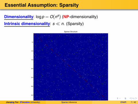
Essential Assumption: Sparsity
Dimensionality: logp = O(na) (NP-dimensionality)
Intrinsic dimensionality: s � n. (Sparsity)
Sparse Structure
50 100 150 200 250 300 350
50
100
150
200
250
300
350
Jianqing Fan (Princeton University) Sparse inference ENAR 7 / 42
Impact of High-dimensionality
Jianqing Fan (Princeton University) Sparse inference ENAR 8 / 42

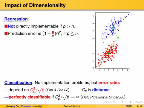
Impact of Dimensionality
Regression:
�Not directly implementable if p > n.
�Prediction error is (1+ pn)2, if p ≤ n.
−2 −1 0 1 2 3 4
−2
−1
01
23
45
?
Classification: No implementation problems, but error rates
—depend on C2p/√
p (Fan & Fan 08), Cp is distance.
—perfectly classifiable if C2p/√
p → (Hall, Pittelkow & Ghosh,08).
Jianqing Fan (Princeton University) Sparse inference ENAR 9 / 42
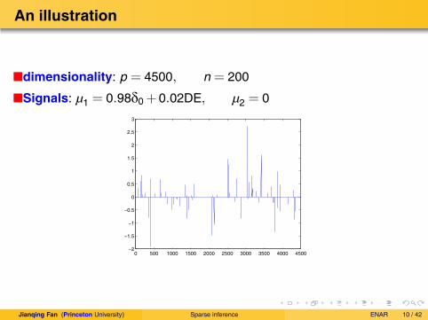
An illustration
�dimensionality: p = 4500, n = 200
�Signals: μ1 = 0.980 +0.02DE, μ2 = 0
0 500 1000 1500 2000 2500 3000 3500 4000 4500−2
−1.5
−1
−0.5
0
0.5
1
1.5
2
2.5
3
Jianqing Fan (Princeton University) Sparse inference ENAR 10 / 42
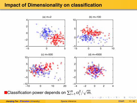
Impact of Dimensionality on classification
−5 0 5−4
−2
0
2
4(a) m=2
−5 0 5 10−5
0
5
10(b) m=100
−10 0 10 20−10
−5
0
5
10(c) m=500
−4 −2 0 2 4−4
−2
0
2
4(d) m=4500
�Classification power depends on mi=12
i /√
m.
Jianqing Fan (Princeton University) Sparse inference ENAR 11 / 42
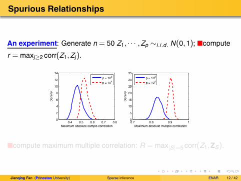
Spurious Relationships
An experiment: Generate n = 50 Z1, · · · ,Zp ∼i.i.d. N(0,1); �compute
r = maxj≥2 corr(Z1,Zj).
0.4 0.5 0.6 0.7 0.80
2
4
6
8
10
12
14
Maximum absolute sample correlation
Den
sity
0.7 0.8 0.9 10
5
10
15
20
25
30
35
Maximum absolute multiple correlationD
ensi
ty
p = 103
p = 104p = 103
p = 104
�compute maximum multiple correlation: R = max|S|=5 corr(Z1,ZS).
Jianqing Fan (Princeton University) Sparse inference ENAR 12 / 42
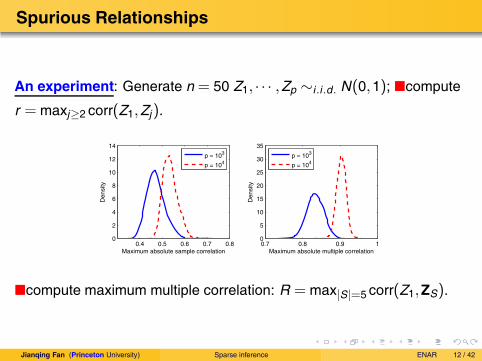
False Outcomes
Scientific implication: If Z1 is responsible for breast cancer, but we
can also discover other 5 genes, indep of outcome!
False statistical inferences: If Y = Z1 and fit
Y = ZTS+ ,
the residual variance
2 =RSS
n−|S| ≈ (1−0.92)× 49
45≈ 0.2,
� is deflation by a factor of more than 1/2
�more variables to be called “statistically significant”.
Jianqing Fan (Princeton University) Sparse inference ENAR 13 / 42
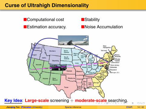
Curse of Ultrahigh Dimensionality
�Computational cost �Stability
�Estimation accuracy. �Noise Accumulation
Key Idea: Large-scale screening + moderate-scale searching.Jianqing Fan (Princeton University) Sparse inference ENAR 14 / 42

The ISIS Method
a two-scale framework
Jianqing Fan (Princeton University) Sparse inference ENAR 15 / 42

Hydrogen Atom: Large scale-screening
Indep learning: Feature ranking by Marginal correlation (Fan & Lv, 08) or
generalized correlation (Hall & Miller, 09);
All possible variables Independence Screening
Classification: Feature ranking by two-sample t-tests or other tests
(Tibshirani, et al, 03; Fan and Fan, 2008).
Jianqing Fan (Princeton University) Sparse inference ENAR 16 / 42
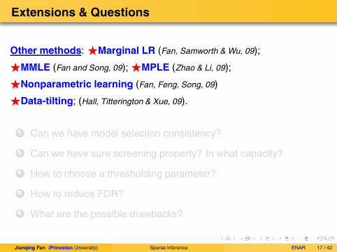
Extensions & Questions
Other methods: �Marginal LR (Fan, Samworth & Wu, 09);
�MMLE (Fan and Song, 09); �MPLE (Zhao & Li, 09);
�Nonparametric learning (Fan, Feng, Song, 09)
�Data-tilting; (Hall, Titterington & Xue, 09).
1 Can we have model selection consistency?
2 Can we have sure screening property? In what capacity?
3 How to choose a thresholding parameter?
4 How to reduce FDR?
5 What are the possible drawbacks?
Jianqing Fan (Princeton University) Sparse inference ENAR 17 / 42
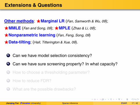
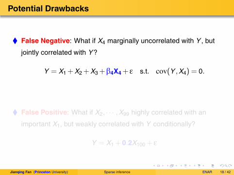
Potential Drawbacks
� False Negative: What if X4 marginally uncorrelated with Y , but
jointly correlated with Y?
Y = X1 +X2 +X3 +4X4 + s.t. cov(Y ,X4) = 0.
� False Positive: What if X2, · · · ,X99 highly correlated with an
important X1, but weakly correlated with Y conditionally?
Y = X1 +0.2X100 +
Jianqing Fan (Princeton University) Sparse inference ENAR 18 / 42

Oxygen Atom: Penalized likelihood estimation
Q() = n−1ni=1 L(Yi ,xT
i,d)+dj=1 p(|j |)
�Simultaneously estimate coefs and choose variables.
Independence Screening Moderate−scale Selection
How high dimensionality can such methods handle?
What is the role of penalty functions?
Does it possess an oracle property? How to compute?Jianqing Fan (Princeton University) Sparse inference ENAR 19 / 42
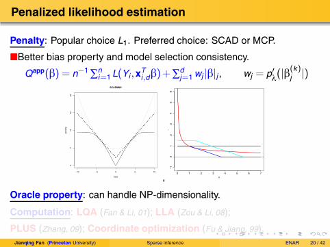
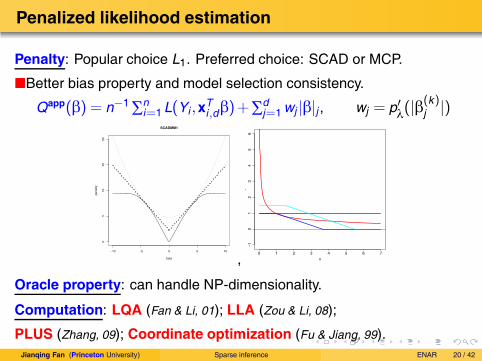
Penalized likelihood estimation
Penalty: Popular choice L1. Preferred choice: SCAD or MCP.
�Better bias property and model selection consistency.
Qapp() = n−1ni=1 L(Yi ,xT
i,d)+dj=1 wj ||j , wj = p′(|
(k)j |)
−10 −5 0 5 10
05
1015
20
SCADMM1
beta
pena
lty
,0 1 2 3 4 5 6 7
−1
01
23
45
6
x
y
Oracle property: can handle NP-dimensionality.
Computation: LQA (Fan & Li, 01); LLA (Zou & Li, 08);
PLUS (Zhang, 09); Coordinate optimization (Fu & Jiang, 99).Jianqing Fan (Princeton University) Sparse inference ENAR 20 / 42

Carbon Atom
Iterative application of
large-scale screening and
moderate-scale selection.
d p
SIS
SCADMCP
LASSODS
�ISIS ((Fan & Lv, 08; Fan, Samworth & Wu, 09)), available in R.
Jianqing Fan (Princeton University) Sparse inference ENAR 21 / 42
Iterative conditional feature selection
1 �(Large-scale screening): Apply SIS to pick a set A1;
�(Moderate-scale selection): Employ a penalized likelihood to
select a subset M1 of these indices.
2 (Large-scale screening): Rank features according to the
additional (conditional) contribution:
L(2)j = min
0,M1,j
n−1n
i=1
L(Yi ,0 +xTi,M1
M1+Xijj),
resulting in A2.
—Improvement of residual approach (FL 08): M1= M1
.
Jianqing Fan (Princeton University) Sparse inference ENAR 22 / 42

Illustration of ISIS
All candidates Conditional Screening
Moderate−scale selection All candidates
Jianqing Fan (Princeton University) Sparse inference ENAR 23 / 42

Jianqing Fan (Princeton University) Sparse inference ENAR 24 / 42

Iterative feature selection (II)
3 (Moderate-scale selection): Minimize wrt M1, A2
n
i=1
L(Yi ,0 +xTi,M1
M1+xT
i,A2A2
)+ j∈M1∪A2
p(|j |),
resulting in M2
—Allow deletion, improvement over ISIS (Fan and Lv, 08).
4 Repeat Steps 1–3 until |M�| = d (prescribed) or M� =M�−1.
d p
SIS
SCADMCP
LASSODS
Jianqing Fan (Princeton University) Sparse inference ENAR 25 / 42

Applicability of ISIS idea
The idea of ISIS is widely applicable. It can be applied to
Classification (Fan, Samworth, & Wu, 09).
Survival analysis (Zhao & Li, 09; Fan, Feng, & Wu, 09).
Nonparametric learning (Fan, Feng, & Song, 09).
Robust and quantile regression (Bradic, Fan, & Wang, 09)
Jianqing Fan (Princeton University) Sparse inference ENAR 26 / 42

Sparse Survival Analysis
Jianqing Fan (Princeton University) Sparse inference ENAR 27 / 42
Hazard regression model
Notation:
Survival time: T . Censoring time: C.
Observation time: Y = min(T ,C)
Censoring indicator = I(T ≤ C).
Covariates: X = (X1,X2, · · · ,Xp)T .
Cox’s proportional hazards model (Cox, 1972 & 1975):
h(t|x) = h0(t)Ψ(x) = h0(t)exp(xT). � sparse.
Jianqing Fan (Princeton University) Sparse inference ENAR 28 / 42
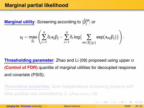
Marginal partial likelihood
Marginal utility: Screening according to |Mj | or
uj = maxj
(n
i=1
i xijj −n
i=1
i log{ m∈R (yi)
exp(xmjj)})
.
Thresholding parameter: Zhao and Li (09) proposed using upper (Control of FDR) quantile of marginal utilities for decoupled response
and covariate (PSIS).
Theoretical properties: sure independence screening property with
false positive rate controlled by . (Zhao and Li, 09)
Jianqing Fan (Princeton University) Sparse inference ENAR 29 / 42

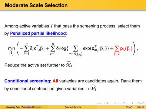
Moderate Scale Selection
Among active variables I that pass the screening process, select them
by Penalized partial likelihood:
minI
(−
n
i=1
ixTI ,iI +
n
i=1
i log{ m∈R (yi)
exp(xTm,II )}+
j∈Ip(j)
),
Reduce the active set further to M1.
Conditional screening: All variables are candidates again. Rank them
by conditional contribution given variables in M1.
Jianqing Fan (Princeton University) Sparse inference ENAR 30 / 42

Simulation Studies
Fan, Feng and Wu (2010)
Jianqing Fan (Princeton University) Sparse inference ENAR 31 / 42

Simulation settings
n = 300 and p = 400, baseline hazard h0(t) = 0.1.
Designs: X1, · · · ,Xp are normal, equally correlated.
� Case 1: = 0.
� Case 2: = 0.5.
� Case 3: = 1/√
2.
� Case 4: case 3 + an indep variable.
Easy to difficulty: case 1 to case 4.
Hidden signature variable: Large impact but indep. of outcome.
Jianqing Fan (Princeton University) Sparse inference ENAR 32 / 42

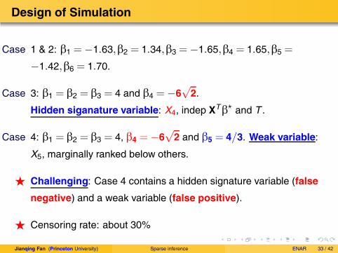
Design of Simulation
Case 1 & 2: 1 = −1.63,2 = 1.34,3 = −1.65,4 = 1.65,5 =
−1.42,6 = 1.70.
Case 3: 1 = 2 = 3 = 4 and 4 = −6√
2.
Hidden siganature variable: X4, indep XT� and T .
Case 4: 1 = 2 = 3 = 4, 4 = −6√
2 and 5 = 4/3. Weak variable:
X5, marginally ranked below others.
� Challenging: Case 4 contains a hidden signature variable (false
negative) and a weak variable (false positive).
� Censoring rate: about 30%
Jianqing Fan (Princeton University) Sparse inference ENAR 33 / 42
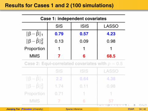
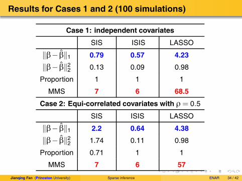
Results for Cases 1 and 2 (100 simulations)
Case 1: independent covariates
SIS ISIS LASSO
‖− ‖1 0.79 0.57 4.23
‖− ‖22 0.13 0.09 0.98
Proportion 1 1 1
MMS 7 6 68.5
Case 2: Equi-correlated covariates with = 0.5
SIS ISIS LASSO
‖− ‖1 2.2 0.64 4.38
‖− ‖22 1.74 0.11 0.98
Proportion 0.71 1 1
MMS 7 6 57
Jianqing Fan (Princeton University) Sparse inference ENAR 34 / 42
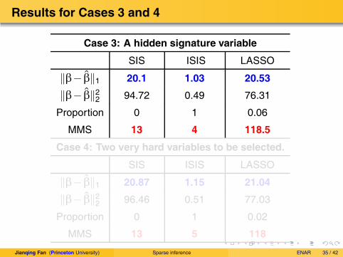
Results for Cases 3 and 4
Case 3: A hidden signature variable
SIS ISIS LASSO
‖− ‖1 20.1 1.03 20.53
‖− ‖22 94.72 0.49 76.31
Proportion 0 1 0.06
MMS 13 4 118.5
Case 4: Two very hard variables to be selected.
SIS ISIS LASSO
‖− ‖1 20.87 1.15 21.04
‖− ‖22 96.46 0.51 77.03
Proportion 0 1 0.02
MMS 13 5 118
Jianqing Fan (Princeton University) Sparse inference ENAR 35 / 42
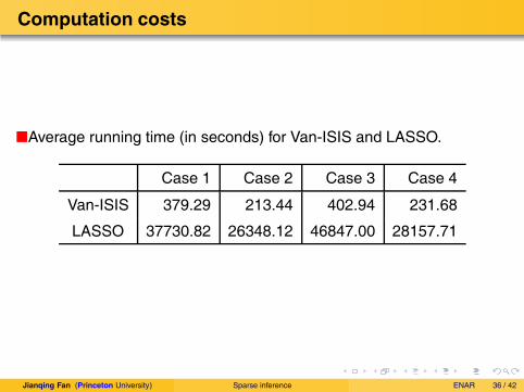
Computation costs
�Average running time (in seconds) for Van-ISIS and LASSO.
Case 1 Case 2 Case 3 Case 4
Van-ISIS 379.29 213.44 402.94 231.68
LASSO 37730.82 26348.12 46847.00 28157.71
Jianqing Fan (Princeton University) Sparse inference ENAR 36 / 42

Cases 2 and 4 with p = 1000
Case 2 with p = 1000 and n = 400
SIS ISIS
‖− ‖1 1.53 0.52
‖− ‖22 0.9 0.07
Proportion 0.82 1
MMS 8 6
Case 4 with p = 1000 and n = 400
SIS ISIS
‖− ‖1 20.88 0.99
‖− ‖22 93.53 0.39
Proportion 0 1
MMS 16 5
Jianqing Fan (Princeton University) Sparse inference ENAR 37 / 42

Cases 2 and 4 with p = 1000
Case 2 with p = 1000 and n = 400
SIS ISIS
‖− ‖1 1.53 0.52
‖− ‖22 0.9 0.07
Proportion 0.82 1
MMS 8 6
Case 4 with p = 1000 and n = 400
SIS ISIS
‖− ‖1 20.88 0.99
‖− ‖22 93.53 0.39
Proportion 0 1
MMS 16 5
Jianqing Fan (Princeton University) Sparse inference ENAR 37 / 42

An Application
Fan, Feng and Wu (2010)
Jianqing Fan (Princeton University) Sparse inference ENAR 38 / 42
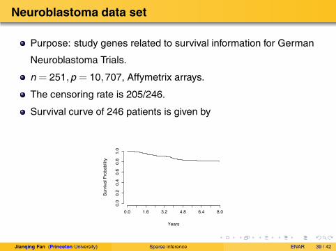
Neuroblastoma data set
Purpose: study genes related to survival information for German
Neuroblastoma Trials.
n = 251,p = 10,707, Affymetrix arrays.
The censoring rate is 205/246.
Survival curve of 246 patients is given by
Years
Sur
viva
l Pro
babi
lity
0.0 1.6 3.2 4.8 6.4 8.0
0.0
0.2
0.4
0.6
0.8
1.0
Jianqing Fan (Princeton University) Sparse inference ENAR 39 / 42
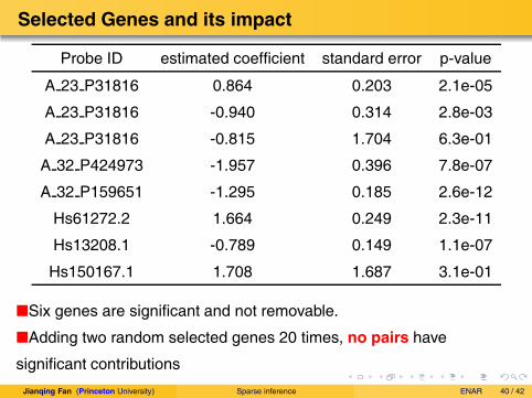
Selected Genes and its impact
Probe ID estimated coefficient standard error p-value
A 23 P31816 0.864 0.203 2.1e-05
A 23 P31816 -0.940 0.314 2.8e-03
A 23 P31816 -0.815 1.704 6.3e-01
A 32 P424973 -1.957 0.396 7.8e-07
A 32 P159651 -1.295 0.185 2.6e-12
Hs61272.2 1.664 0.249 2.3e-11
Hs13208.1 -0.789 0.149 1.1e-07
Hs150167.1 1.708 1.687 3.1e-01
�Six genes are significant and not removable.
�Adding two random selected genes 20 times, no pairs have
significant contributions
Jianqing Fan (Princeton University) Sparse inference ENAR 40 / 42
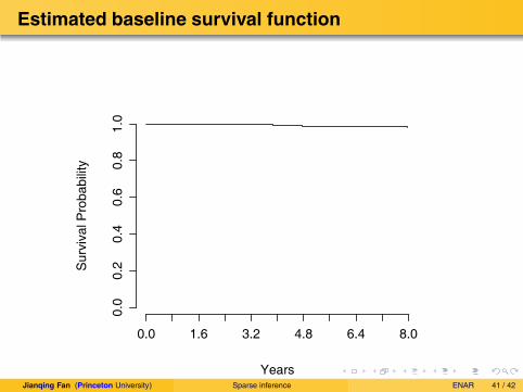
Estimated baseline survival function
Years
Sur
viva
l Pro
babi
lity
0.0 1.6 3.2 4.8 6.4 8.0
0.0
0.2
0.4
0.6
0.8
1.0
Jianqing Fan (Princeton University) Sparse inference ENAR 41 / 42
Acknowledgement
Thank YouIn collaboration with
� Yang Feng (Princeton University; FFW, 2009)
� Jinchi Lv (University of Southern California; Fan & Lv; 2008)
� Richard Samworth (Cambridge University; FSW, 2009).
� Rui Song (Colorado State University, Fan & Song, 2009).
� Yichao Wu (North Carolina State University, FSW, 2009).Jianqing Fan (Princeton University) Sparse inference ENAR 42 / 42