Isentropic transport and the seasonal cycle amplitude of CO2

Journal of Geophysical Research: Atmospheres

Isentropic transport and the seasonal cycle amplitude of CO2

Elizabeth A. Barnes1, Nicholas Parazoo2,3, Clara Orbe4,5, and A. Scott Denning1

1Department of Atmospheric Science, Colorado State University, Fort Collins, Colorado, USA, 2Jet Propulsion Laboratory,California Institute of Technology, Pasadena, California, USA, 3Joint Institute for Regional Earth System Science andEngineering, University of California, Los Angeles, California, USA, 4Department of Earth and Planetary Sciences, GoddardEarth Sciences Technology and Research (GESTAR)/Johns Hopkins University, Baltimore, Maryland, USA, 5NASA GoddardSpace Flight Center, Greenbelt, Maryland, USA

Abstract Carbon-concentration feedbacks and carbon-climate feedbacks constitute one of the largestsources of uncertainty in future climate. Since the beginning of the modern atmospheric CO2 record,seasonal variations in CO2 have been recognized as a signal of the metabolism of land ecosystems, andquantitative attribution of changes in the seasonal cycle amplitude (SCA) of CO2 to ecosystem processesis critical for understanding and projecting carbon-climate feedbacks far into the 21st Century. Here theimpact of surface carbon fluxes on the SCA of CO2 throughout the Northern Hemisphere troposphere isinvestigated, paying particular attention to isentropic transport across latitudes. The analysis includes botha chemical transport model GOES-Chem and an idealized tracer in a gray-radiation aquaplanet. The resultsof the study can be summarized by two main conclusions: (1) the SCA of CO2 roughly follows surfacesof constant potential temperature, which can explain the observed increase in SCA with latitude alongpressure surfaces and (2) increasing seasonal fluxes in lower latitudes have a larger impact on the SCA ofCO2 throughout most of the troposphere compared to increasing seasonal fluxes in higher latitudes. Theseresults provide strong evidence that recently observed changes in the SCA of CO2 at high northern latitudes(poleward of 60∘N) are likely driven by changes in midlatitude surface fluxes, rather than changesin Arctic fluxes.

1. Introduction and Motivation

Carbon-concentration feedbacks and carbon-climate feedbacks constitute one of the largest sources of uncer-tainty in future climate [Gregory et al., 2009]. Land CO2 uptake by ecosystem production is enhanced by CO2

fertilization [Luo et al., 2006], but CO2 release due to decomposition is enhanced by warming [Hopkins et al.,2012]. Changes in nutrient cycling [LeBauer and Treseder, 2008] and land use [Shevliakova et al., 2009] alterseasonal and long-term carbon storage on land. Long-term warming and drought also change the distribu-tion of vegetation [Cramer et al., 2001] and may contribute to substantial losses of carbon from biomass inforests [Cox et al., 2004] and permafrost [Schuur et al., 2013]. Terrestrial carbon cycle models show substan-tial differences in the magnitude and (at times) sign of the impact that these various ecosystem processeshave had over recent decades on the atmospheric CO2 budget [Huntzinger et al., 2013; Fisher et al., 2014b; Tianet al., 2015]. Uncertainty in the future of carbon-climate feedbacks on land accounts for more than 2 W/m2 ofradiative forcing given identical top-of-atmosphere forcing among coupled carbon-climate models used inthe Fifth Assessment of the Intergovernmental Panel on Climate Change [Arora et al., 2013; Wenzel et al., 2014;Hoffman et al., 2014].

The seasonal cycle of near-surface CO2 from the NOAA Marine Boundary Layer Reference data set (seesection 2.1 for details) is shown in Figure 1a and exhibits enhanced concentrations in the cool season dueto soil respiration and decreased concentrations in the warm season due to net uptake by the biosphere.Quantitative attribution of changes in the seasonal cycle amplitude (SCA; peak to trough differences inFigure 1a) of CO2 to ecosystem processes is critical for testing models of carbon-climate feedback in the 21stcentury. Since the beginning of the modern atmospheric CO2 record, seasonal variations have been recog-nized as a signal of the metabolism of land ecosystems [Keeling, 1960]. The quantitative relationship betweenSCA and its underlying biological drivers has been studied using tracer transport models since the 1980s[Pearman and Hyson, 1980; Fung et al., 1983, 1987; Randerson et al., 1997]. The SCA of CO2 has been increasingfor decades across the Northern Hemisphere, and this amplification has long been attributed to intensification

RESEARCH ARTICLE10.1002/2016JD025109

Key Points:• The seasonal cycle amplitude (SCA)

of CO2 roughly follows isentropicsurfaces

• Changes in lower-latitude seasonalfluxes impact the SCA more thanchanges in higher-latitude fluxes

• The seasonality of the circulation canaccount for 10–20% of the SCA of anidealized CO2 tracer

Correspondence to:E. A. Barnes,[email protected]

Citation:Barnes, E. A., N. Parazoo, C. Orbe,and A. S. Denning (2016),Isentropic transport and theseasonal cycle amplitude ofCO2, J. Geophys. Res. Atmos.,121, doi:10.1002/2016JD025109.

Received 16 MAR 2016

Accepted 18 JUN 2016

Accepted article online 25 JUN 2016

©2016. American Geophysical Union.All Rights Reserved.

BARNES ET AL. SEASONAL CYCLE AMPLITUDE OF CO2 1

http://publications.agu.org/journals/

http://onlinelibrary.wiley.com/journal/10.1002/(ISSN)2169-8996

http://dx.doi.org/10.1002/2016JD025109

Journal of Geophysical Research: Atmospheres 10.1002/2016JD025109

Figure 1. NOAA Marine Boundary Layer Reference 2009–2013 zonally averaged CO2 (a) seasonal cycle and (b) seasonalcycle amplitude as a function of latitude.

of carbon metabolism on land [Bacastow and Keeling, 1981]. More recently, a number of studies have arguedthat the amplification of the seasonal cycle of CO2 at high-latitude stations and from aircraft sampling reflectsa response of northern ecosystems to climate change [Graven et al., 2013; Forkel et al., 2016] or to enhancedagricultural productivity [Gray et al., 2014; Zeng et al., 2014]. Models of changes in carbon cycling in boreal andArctic ecosystems are especially divergent [Fisher et al., 2014a], which has led to a strong research emphasison detailed regional measurements of atmospheric carbon budgets [Miller and Dinardo, 2012].

Attribution of changes in SCA to ecological processes in specific regions requires quantitative treatment ofatmospheric transport. The observed SCA increases almost monotonically with latitude (see Figure 1b), yetbiological productivity has a maximum in the midlatitudes (roughly 30∘N–60 ∘N). Regional CO2 budgetsbased on drawdown or sources in the atmospheric boundary layer show substantial effects of meridionaladvection [Bakwin et al., 2004; Helliker et al., 2004]. Meridional CO2 transport by synoptic weather disturbancesis systematically correlated with ecosystem metabolism on land [Parazoo et al., 2008; Hurwitz et al., 2004] andis acknowledged to play a critical role in determining the seasonal cycle at high latitudes (roughly poleward of60∘N) [Fung et al., 1983; Parazoo et al., 2011]. Attempts to construct regional carbon budgets for high-latitudeecosystems using observations of atmospheric carbon tracers [Chang et al., 2014; Henderson et al., 2015; Karionet al., 2015] require detailed specification of meridional advective fluxes through lateral boundary conditions.Much of this synoptic transport is along surfaces of constant potential temperatures (“isentropic trans-port”), but diabatic processes such as condensation and radiation can also be important in the troposphere[Crawford et al., 2003; Barth et al., 2007; Miyazaki et al., 2008; Pauluis et al., 2010]. Atmospheric transport by syn-optic weather systems is systematically hidden by clouds from space-based observing systems and thus canlead to mischaracterization of seasonal cycles [Corbin et al., 2009].



In this paper, we explore the fundamental relationships between surface carbon fluxes and atmospheric trans-port that can explain the seasonal cycle amplitude of CO2 throughout the troposphere, paying particularattention to isentropic transport across latitudes. Our analysis includes both a widely used transport modelderived from meteorological reanalysis and a much simpler moist aquaplanet that can also capture the rele-vant dynamics. We explore the effect of both surface fluxes and transport to isolate contributions of differentlatitudes and transport processes to the SCA of CO2.

2. Data and Experimental Design2.1. NOAA Marine Boundary Layer ReferenceFigure 1 displays results from the National Oceanic and Atmospheric Administration (NOAA) Greenhouse GasMarine Boundary Layer Reference data set [Dlugokencky et al., 2015]. This data product is derived from weeklyair samples from the NOAA Earth System Research Laboratory Carbon Cycle Cooperative Global Air SamplingNetwork and is smoothed in time and interpolated in space to produce a weekly zonally averaged data setof near-surface CO2 as a function of time and latitude. To be consistent with the model simulations, we onlyanalyze 2009–2013, although we have confirmed that using the entire record of 1979–2014 produces similarresults.

2.2. GEOS-ChemGEOS-Chem is a global 3-D chemical transport model for atmospheric composition that uses GEOS (GoddardEarth Observing System) assimilated meteorological fields from the NASA Global Modeling and AssimilationOffice to simulate global atmospheric composition, including CO2 [Bey et al., 2001]. Dynamics include hori-zontal and vertical advection, turbulent diffusion, and moist convection. We use the CO2 mode which ignoreschemistry but contains atmospheric CO2 fields. GEOS-Chem has been used extensively in studies of atmo-spheric CO2 and quantitative attribution of surface carbon fluxes and compares well against a range of surface,airborne, and satellite CO2 observations [e.g., Parazoo et al., 2013; Wunch et al., 2013; Messerschmidt et al., 2013;Nassar et al., 2010].

2.3. Land Surface FluxesMonthly biological CO2 flux is simulated using the Community Land Model version 4.5 (CLM) [Oleson et al.,2013] using an experimental setup as described in Le Quéré et al. [2015]. CLM is forced by time-varying reanal-ysis meteorology taken from the combined Climatic Research Unit and National Center for EnvironmentalPrediction data set, which merges high-frequency variability from the National Centers for EnvornmentalPrediction-National Center for Atmospheric Research analysis [Kalnay et al., 1996] with the monthly meanclimatologies from the Climatic Research Unit (CRU) temperature and precipitation data sets [Harris et al.,2014]. Monthly fossil fuel emissions are taken from Open-source Data Inventory of Anthropogenic CO2(ODIAC)[Oda and Maksyutov, 2011] and averaged over 2009–2013 to isolate the sensitivity of atmospheric CO2 fieldsto seasonal biosphere exchange. We use GEOS-Chem version v9-01-01 with GEOS-5 fields on a 2∘ × 2.5∘ grid(latitude × longitude) with 47 vertical layers. Simulations are spun up from 2000 to 2008 to establish hemi-spheric gradients. The experiments based on GEOS-Chem and CLM are described in more detail in Parazooet al. [2016]. As we will demonstrate, the modeled CO2 seasonal cycle from our GEOS-Chem/CLM setupcompares well with that from the NOAA Marine Boundary Layer Reference data set.

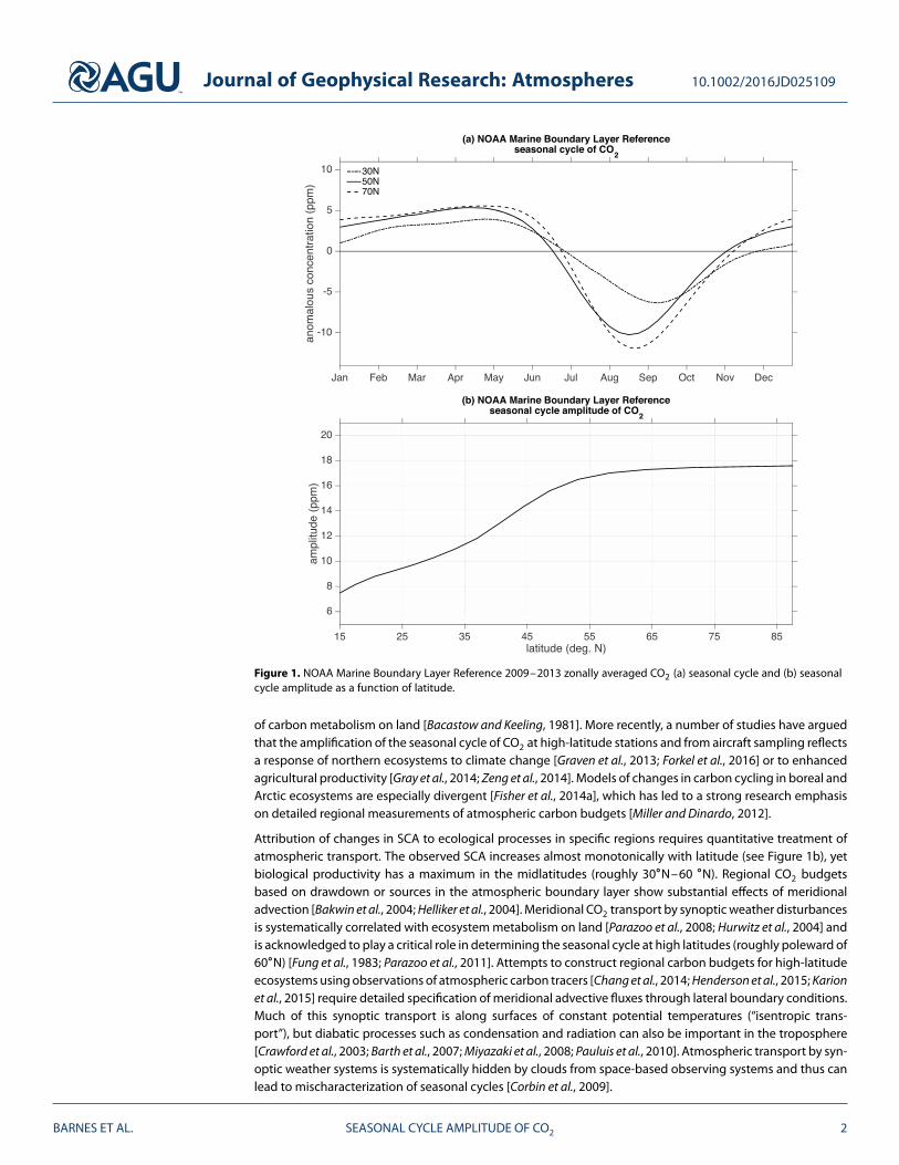
Figure 2 depicts the zonally integrated CO2 fluxes from the land surface to the atmosphere as a function oflatitude and month averaged over the 2009–2013 period from CLM and ODIAC. On average, the land is a netsource of CO2 to the atmosphere (6.54 Pg C yr−1), contributing 9.21 Pg C yr−1 from fossil fuels and removing2.67 Pg C yr−1 from the atmosphere through biosphere uptake. However, biosphere fluxes are strongly sea-sonal. In the winter, the biosphere is a net CO2 source driven by soil respiration, as denoted by the positivefluxes (warm colors). In the summer, the biosphere is a net CO2 sink driven by photosynthesis, as denotedby the negative fluxes (cool colors). Fossil fuel emissions are positive all year, leading to a slightly enhancedwinter source and reduced summer sink.

We note that GEOS-Chem simulations also include a CO2 flux term that accounts for air-sea exchange overthe oceans [Takahashi et al., 2009], which removes an additional 1.43 Pg C yr−1 from the atmosphere, reduc-ing total source emissions to 5.11 Pg C yr−1. Although absorption by the ocean reduces the rate of increase ofatmospheric CO2 concentration, our analysis removes all long-term trends. Furthermore, ocean uptake doesnot have strong seasonality compared to land fluxes. The ocean is therefore not expected to impact our inter-pretation of the climatological seasonal cycle, and as discussed below is not included in simulations with the



Figure 2. Annual average seasonal cycle of the surface fluxes of CO2 as a function of latitude for 2009–2013 assimulated by CLM.

idealized general circulation model (GCM). We finally note that simplifications have been made when cou-pling CLM to GEOS-Chem, for example, not including the diurnal cycle of the fluxes. However, the purposeof this study is to explore fundamental dynamical transport mechanisms, and as we will show, the relevanttransport pathways are well captured by the GEOS-Chem and idealized model simulations.

2.4. Idealized GCMWe use the gray-radiation aquaplanet general circulation model (GCM) described in Frierson et al. [2006]. Themodel physics includes gray radiative transfer such that water vapor has no effect on the radiative fluxes butcan still influence the climate through latent heating and cooling. There are no clouds in this model, and radia-tive fluxes are a function of temperature only. The surface is a slab mixed layer ocean that is zonally symmetric(i.e., no topography). As in Frierson et al. [2006], we run the model without a convective parameterization usinglarge-scale condensation only. All parameters are defined as in Frierson et al. [2006] except that their modelconfiguration did not include a seasonal cycle. Thus, we simulate a seasonal cycle by varying the insolationas a function of the day of the year, using a 360 day calendar. Details of this procedure are provided in theappendix. The model is run at a horizontal resolution of T42 with 25 vertical levels and a time step of 900 s.The model does not simulate a realistic stratospheric circulation, which is intentional on our part, as we wishto focus exclusively on the tropospheric transport component of the SCA of the idealized tracers.

The aim of this study is to explore the fundamental relationship between the seasonal surface carbon fluxesand the tropospheric transport pathways that drive the seasonal cycle amplitude of CO2 throughout the tro-posphere. The idealized model is an excellent tool for studying these basic transport mechanisms as it isolatesthe fundamental dynamics by removing many of the additional complexities of the real world. As we willshow, even with these simplifications, the idealized model captures the observed seasonal behavior of CO2

and thus is used to study the mechanisms responsible.

2.5. Tracer SetupAn idealized tracer is added to the gray aquaplanet, with surface sources and sinks driven by the monthly sur-face fluxes depicted in Figure 2. Specifically, the sources and sinks of the tracer are confined to the bottomlayer of the model, are zonally symmetric, and are added (or subtracted) to each air parcel that enters the bot-tom boundary. The model integrates the tracer in units of mixing ratio, and so, the fluxes were converted intoa mixing ratio per time step before being input into the model. Note that converting from a flux to a mixingratio requires calculating the mass of air in the bottom model layer. Since our model has no topography, wehave confirmed that the results are for all purposes identical if one assumes a constant mass of the bottomlayer of the model, which is done here for simplicity. The idealized tracer is initialized at the start of the simula-tion and is integrated using a Lin-Rood semi-Lagrangian scheme [Lin and Rood, 1996] for horizontal advectionand a finite-volume parabolic scheme for the vertical advection [Lagenhorst, 2005], with no explicit diffusionapplied to the tracer. The model is integrated with a global “mass fixer” to ensure that the global tracer mass



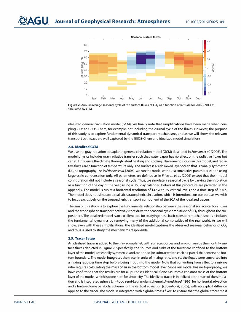
Figure 3. (a) The zonal mean concentration of the idealized tracer as a function of time at 60∘N. (b) The climatologicalmean seasonal cycle of the idealized tracer at 60∘N. The dashed line denotes the smoothed cycle (see text for details),and the circles denote the maximum (red) and minimum (blue) of the smoothed curves.

remains unchanged after every application of the advection operator (before the addition/removal by thesurface source). This idealized tracer is identical to that used by Orbe et al. [2013] in a dry version of a similaridealized GCM but with different sources and sinks.

Integrating the fluxes in Figure 2 over an entire year yields a positive total flux driven by fossil fuel emissions.This drives a linear increase in the tracer with time. Our results are insensitive to this increase, and all of thesubsequent analysis is performed on the detrended time series, as shown in Figure 3a for the zonally averagedtracer at 60∘N for two different pressure levels. A seasonal cycle is evident in Figure 3a, with the seasonal cycleamplitude (peak to trough) being larger at 750 hPa (purple) compared to 350 hPa (green). The details of thisseasonal cycle will be the focus of the analysis in the subsequent sections.

Our goal is to study the transport pathways that determine the overall structure of the SCA of CO2 through-out the troposphere. Thus, to easily compare the structure of the SCA between the idealized model andGEOS-Chem simulations, rather than the actual magnitudes which differ due to the different model setupsand assumptions, we scale all of the idealized tracer concentrations in the idealized simulations by a singlevalue to easily compare them with those from GEOS-Chem. The scaling value used is the SCA at 50∘N and750 hPa in the GEOS-Chem Control simulation, so that the idealized model and GEOS-Chem have the sameSCA at this location, and thus, their relative variations with latitude can be easily compared. We note that ourconclusions do not change if a different location is used to define the scaling.

2.6. ExperimentsFive experiments were explored with the idealized aquaplanet. Each experiment is composed of 54 year simu-lations with the first 4 years discarded for spin-up leaving 50 years for analysis. A summary of each experiment



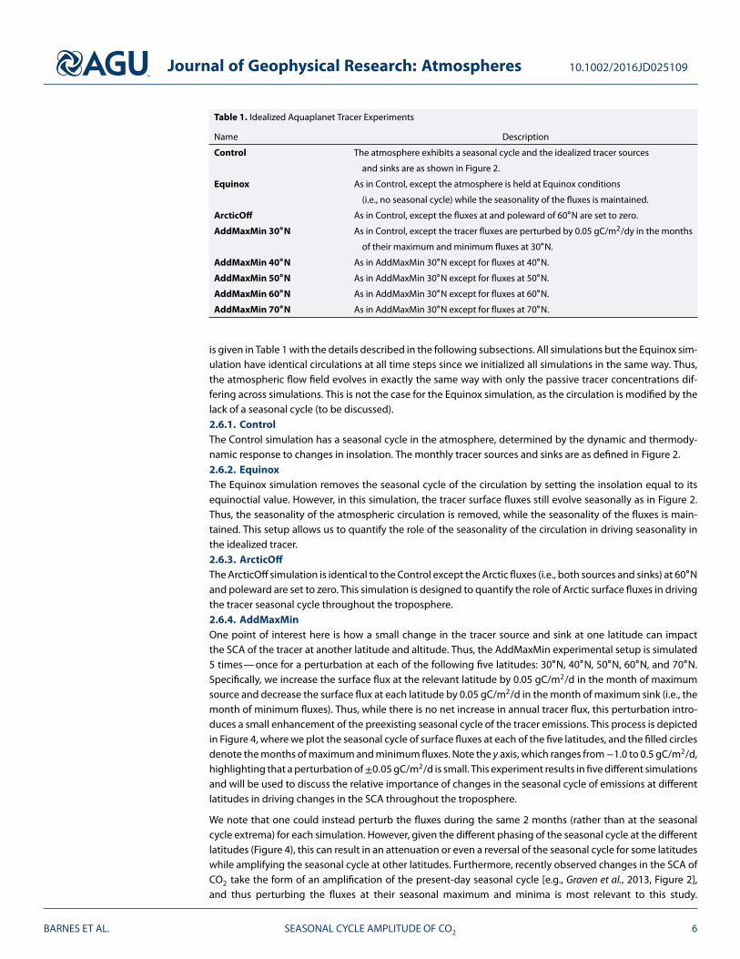
Table 1. Idealized Aquaplanet Tracer Experiments

Name Description

Control The atmosphere exhibits a seasonal cycle and the idealized tracer sources

and sinks are as shown in Figure 2.

Equinox As in Control, except the atmosphere is held at Equinox conditions

(i.e., no seasonal cycle) while the seasonality of the fluxes is maintained.

ArcticOff As in Control, except the fluxes at and poleward of 60∘N are set to zero.

AddMaxMin 30∘N As in Control, except the tracer fluxes are perturbed by 0.05 gC/m2/dy in the months

of their maximum and minimum fluxes at 30∘N.

AddMaxMin 40∘N As in AddMaxMin 30∘N except for fluxes at 40∘N.




is given in Table 1 with the details described in the following subsections. All simulations but the Equinox sim-ulation have identical circulations at all time steps since we initialized all simulations in the same way. Thus,the atmospheric flow field evolves in exactly the same way with only the passive tracer concentrations dif-fering across simulations. This is not the case for the Equinox simulation, as the circulation is modified by thelack of a seasonal cycle (to be discussed).2.6.1. ControlThe Control simulation has a seasonal cycle in the atmosphere, determined by the dynamic and thermody-namic response to changes in insolation. The monthly tracer sources and sinks are as defined in Figure 2.2.6.2. EquinoxThe Equinox simulation removes the seasonal cycle of the circulation by setting the insolation equal to itsequinoctial value. However, in this simulation, the tracer surface fluxes still evolve seasonally as in Figure 2.Thus, the seasonality of the atmospheric circulation is removed, while the seasonality of the fluxes is main-tained. This setup allows us to quantify the role of the seasonality of the circulation in driving seasonality inthe idealized tracer.2.6.3. ArcticOffThe ArcticOff simulation is identical to the Control except the Arctic fluxes (i.e., both sources and sinks) at 60∘Nand poleward are set to zero. This simulation is designed to quantify the role of Arctic surface fluxes in drivingthe tracer seasonal cycle throughout the troposphere.2.6.4. AddMaxMinOne point of interest here is how a small change in the tracer source and sink at one latitude can impactthe SCA of the tracer at another latitude and altitude. Thus, the AddMaxMin experimental setup is simulated5 times—once for a perturbation at each of the following five latitudes: 30∘N, 40∘N, 50∘N, 60∘N, and 70∘N.Specifically, we increase the surface flux at the relevant latitude by 0.05 gC/m2/d in the month of maximumsource and decrease the surface flux at each latitude by 0.05 gC/m2/d in the month of maximum sink (i.e., themonth of minimum fluxes). Thus, while there is no net increase in annual tracer flux, this perturbation intro-duces a small enhancement of the preexisting seasonal cycle of the tracer emissions. This process is depictedin Figure 4, where we plot the seasonal cycle of surface fluxes at each of the five latitudes, and the filled circlesdenote the months of maximum and minimum fluxes. Note the y axis, which ranges from−1.0 to 0.5 gC/m2/d,highlighting that a perturbation of±0.05 gC/m2/d is small. This experiment results in five different simulationsand will be used to discuss the relative importance of changes in the seasonal cycle of emissions at differentlatitudes in driving changes in the SCA throughout the troposphere.

We note that one could instead perturb the fluxes during the same 2 months (rather than at the seasonalcycle extrema) for each simulation. However, given the different phasing of the seasonal cycle at the differentlatitudes (Figure 4), this can result in an attenuation or even a reversal of the seasonal cycle for some latitudeswhile amplifying the seasonal cycle at other latitudes. Furthermore, recently observed changes in the SCA ofCO2 take the form of an amplification of the present-day seasonal cycle [e.g., Graven et al., 2013, Figure 2],and thus perturbing the fluxes at their seasonal maximum and minima is most relevant to this study.



Figure 4. Surface fluxes of the idealized tracer showing the maximum and minimum months. See text for additionaldetails.

Finally, we note that Keppel-Aleks et al. [2011] performed similar experiments to explore the response of thetotal-column SCA to perturbations of surface fluxes at different latitudes except that they scaled each lati-tude’s perturbation so that the Northern Hemisphere net primary production increased by 25% in every case.We have intentionally used a fixed flux perturbation (i.e., ±0.05 gC/m2/d) to test how the SCA may respond ifeach meter squared of biosphere underwent the same physical change at each of the five latitudes.

2.7. Calculation of the Seasonal Cycle Amplitude (SCA)It is evident from Figure 3a that the tracer exhibits a strong seasonal cycle and that the seasonal cycle ampli-tude varies throughout the troposphere. We quantify the SCA by calculating the smoothed climatologicalseasonal cycle of the zonally averaged tracer concentrations at every pressure level and latitude. Figure 3bshows an example of this seasonal cycle at 60∘N for the lower troposphere (750 hPa; purple) and the upper tro-posphere (350 hPa; green). The solid lines in Figure 3b denote the raw curves, and the dashed lines denote thecurves smoothed with a moving average window of length 31 days applied forward and backward. The redand blue dots denote the maximum and minimum concentrations, respectively, over the smoothed seasonalcycle at each point, and the SCA is defined as the difference between these extrema.

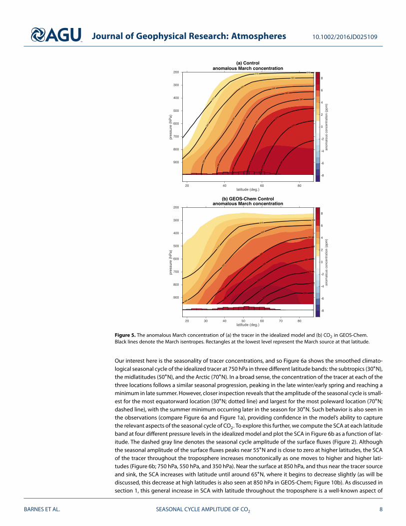
3. Results3.1. Control SimulationThe 50 year mean anomalous March tracer concentrations, defined as the deviation from the 50 year annualmean, are shown in Figure 5a for the Control simulation of the idealized aquaplanet. March is chosen becauselate winter/early spring is when the tracer concentrations are largest throughout the troposphere, consistentwith the timing of when the winter time source has had time to build up tropospheric concentrations, butthe surface sink has not yet appeared (see Figure 2). The March circulation is also representative of the coolseason circulation when poleward isentropic transport by the storm tracks is strongest. The concentrationsare largest near the surface, peaking slightly poleward of the maximum surface source during this month(red rectangles), and decrease as one moves away from the surface. Lines of constant potential tempera-ture (isentropes) are plotted as thick black lines. It is evident that the tracer concentrations roughly followthese isentropic surfaces, sloping upward and poleward, which is expected since isentropic transport by thewinter time midlatitude storm track is known to be an important pathway for the poleward transport ofCO2 [Miyazaki et al., 2008; Parazoo et al., 2011; Keppel-Aleks et al., 2012] and other atmospheric constituents[e.g., Klonecki et al., 2003; Stohl, 2006]. We do note, however, that the concentrations do not align exactlywith the dry isentropes due to cross-isentropic transport induced by, for example, diabatic heating within themidlatitude storm tracks [e.g., Klonecki et al., 2003; Parazoo et al., 2011]. To support the use of such an ide-alized model in properly simulating the transport of CO2, Figure 5b shows the same anomalous March CO2

concentrations from GEOS-Chem. While small differences can certainly be found, the general observationthat the CO2 concentrations peak near the surface just poleward of the maximum source and that the CO2

concentrations slope upward and poleward are clearly evident in both models.



Figure 5. The anomalous March concentration of (a) the tracer in the idealized model and (b) CO2 in GEOS-Chem.Black lines denote the March isentropes. Rectangles at the lowest level represent the March source at that latitude.

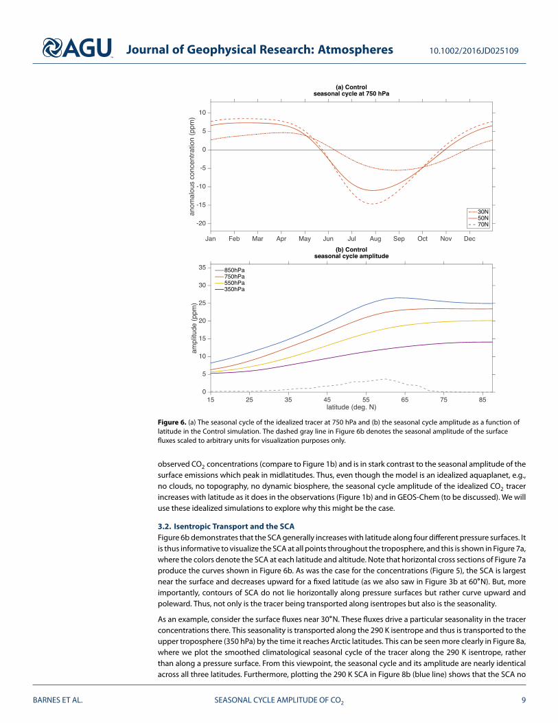
Our interest here is the seasonality of tracer concentrations, and so Figure 6a shows the smoothed climato-logical seasonal cycle of the idealized tracer at 750 hPa in three different latitude bands: the subtropics (30∘N),the midlatitudes (50∘N), and the Arctic (70∘N). In a broad sense, the concentration of the tracer at each of thethree locations follows a similar seasonal progression, peaking in the late winter/early spring and reaching aminimum in late summer. However, closer inspection reveals that the amplitude of the seasonal cycle is small-est for the most equatorward location (30∘N; dotted line) and largest for the most poleward location (70∘N;dashed line), with the summer minimum occurring later in the season for 30∘N. Such behavior is also seen inthe observations (compare Figure 6a and Figure 1a), providing confidence in the model’s ability to capturethe relevant aspects of the seasonal cycle of CO2. To explore this further, we compute the SCA at each latitudeband at four different pressure levels in the idealized model and plot the SCA in Figure 6b as a function of lat-itude. The dashed gray line denotes the seasonal cycle amplitude of the surface fluxes (Figure 2). Althoughthe seasonal amplitude of the surface fluxes peaks near 55∘N and is close to zero at higher latitudes, the SCAof the tracer throughout the troposphere increases monotonically as one moves to higher and higher lati-tudes (Figure 6b; 750 hPa, 550 hPa, and 350 hPa). Near the surface at 850 hPa, and thus near the tracer sourceand sink, the SCA increases with latitude until around 65∘N, where it begins to decrease slightly (as will bediscussed, this decrease at high latitudes is also seen at 850 hPa in GEOS-Chem; Figure 10b). As discussed insection 1, this general increase in SCA with latitude throughout the troposphere is a well-known aspect of



Figure 6. (a) The seasonal cycle of the idealized tracer at 750 hPa and (b) the seasonal cycle amplitude as a function oflatitude in the Control simulation. The dashed gray line in Figure 6b denotes the seasonal amplitude of the surfacefluxes scaled to arbitrary units for visualization purposes only.

observed CO2 concentrations (compare to Figure 1b) and is in stark contrast to the seasonal amplitude of thesurface emissions which peak in midlatitudes. Thus, even though the model is an idealized aquaplanet, e.g.,no clouds, no topography, no dynamic biosphere, the seasonal cycle amplitude of the idealized CO2 tracerincreases with latitude as it does in the observations (Figure 1b) and in GEOS-Chem (to be discussed). We willuse these idealized simulations to explore why this might be the case.

3.2. Isentropic Transport and the SCAFigure 6b demonstrates that the SCA generally increases with latitude along four different pressure surfaces. Itis thus informative to visualize the SCA at all points throughout the troposphere, and this is shown in Figure 7a,where the colors denote the SCA at each latitude and altitude. Note that horizontal cross sections of Figure 7aproduce the curves shown in Figure 6b. As was the case for the concentrations (Figure 5), the SCA is largestnear the surface and decreases upward for a fixed latitude (as we also saw in Figure 3b at 60∘N). But, moreimportantly, contours of SCA do not lie horizontally along pressure surfaces but rather curve upward andpoleward. Thus, not only is the tracer being transported along isentropes but also is the seasonality.

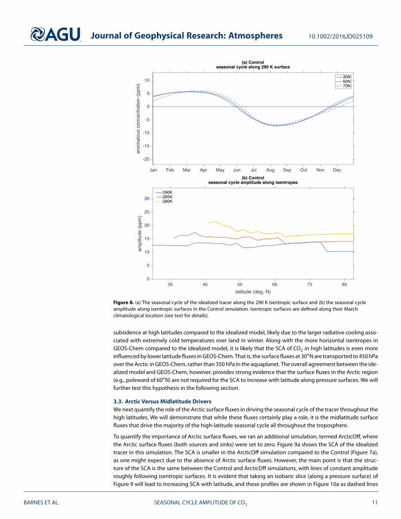
As an example, consider the surface fluxes near 30∘N. These fluxes drive a particular seasonality in the tracerconcentrations there. This seasonality is transported along the 290 K isentrope and thus is transported to theupper troposphere (350 hPa) by the time it reaches Arctic latitudes. This can be seen more clearly in Figure 8a,where we plot the smoothed climatological seasonal cycle of the tracer along the 290 K isentrope, ratherthan along a pressure surface. From this viewpoint, the seasonal cycle and its amplitude are nearly identicalacross all three latitudes. Furthermore, plotting the 290 K SCA in Figure 8b (blue line) shows that the SCA no



Figure 7. Seasonal cycle amplitude of (a) the tracer in the idealized model and (b) CO2 in GEOS-Chem. Black linesdenote the March isentropes. Rectangles at the lowest level represent the average source (red) and sink (blue)throughout the year at that latitude.

longer increases with latitude but rather is nearly constant as expected from Figure 7. The 285 K isentrope(red) also exhibits nearly constant SCAs of the tracer for all latitudes. The constant SCA with latitude begins tobreakdown for the tracer along the 280 K isentrope (yellow) as this isentropic surface is located in the lowertroposphere at high latitudes where cross-isentropic sinking of the tracer (and its seasonality) due to radiativecooling becomes important [e.g., Klonecki et al., 2003; Miyazaki et al., 2008].

The fact that the tracer, and thus its seasonality, is transported to high latitudes along isentropic surfaces canaccount for why the SCA of the tracer increases with latitude along pressure surfaces. Due to the upwardand poleward transport of CO2 along isentropic surfaces, the SCA in the high latitudes is a reflection of thetracer’s surface fluxes farther equatorward. Thus, even though the surface fluxes near the pole are zero, thelargest SCAs are found in the high-latitude troposphere since they correspond to isentropes that intersectthe midlatitude surface in the vicinity of the maximum surface flux seasonality (e.g., 55∘N).

For further support, Figure 7b shows the SCA of CO2 from GEOS-Chem. While our idealized model has no conti-nents or topography and fully determines its own dynamics, GEOS-Chem advects CO2 according to reanalysiswinds and thus includes all of the complexity of the real-world circulation. Comparing the SCAs from theidealized aquaplanet with the GEOS-Chem reveals very similar behavior of the seasonal cycle amplitude,with the SCA sloping up and poleward along isentropic surfaces. GEOS-Chem does exhibit stronger diabatic



Figure 8. (a) The seasonal cycle of the idealized tracer along the 290 K isentropic surface and (b) the seasonal cycleamplitude along isentropic surfaces in the Control simulation. Isentropic surfaces are defined along their Marchclimatological location (see text for details).

subsidence at high latitudes compared to the idealized model, likely due to the larger radiative cooling asso-ciated with extremely cold temperatures over land in winter. Along with the more horizontal isentropes inGEOS-Chem compared to the idealized model, it is likely that the SCA of CO2 in high latitudes is even moreinfluenced by lower latitude fluxes in GEOS-Chem. That is, the surface fluxes at 30∘N are transported to 450 hPaover the Arctic in GEOS-Chem, rather than 350 hPa in the aquaplanet. The overall agreement between the ide-alized model and GEOS-Chem, however, provides strong evidence that the surface fluxes in the Arctic region(e.g., poleward of 60∘N) are not required for the SCA to increase with latitude along pressure surfaces. We willfurther test this hypothesis in the following section.

3.3. Arctic Versus Midlatitude DriversWe next quantify the role of the Arctic surface fluxes in driving the seasonal cycle of the tracer throughout thehigh latitudes. We will demonstrate that while these fluxes certainly play a role, it is the midlatitude surfacefluxes that drive the majority of the high-latitude seasonal cycle all throughout the troposphere.

To quantify the importance of Arctic surface fluxes, we ran an additional simulation, termed ArcticOff, wherethe Arctic surface fluxes (both sources and sinks) were set to zero. Figure 9a shows the SCA of the idealizedtracer in this simulation. The SCA is smaller in the ArcticOff simulation compared to the Control (Figure 7a),as one might expect due to the absence of Arctic surface fluxes. However, the main point is that the struc-ture of the SCA is the same between the Control and ArcticOff simulations, with lines of constant amplituderoughly following isentropic surfaces. It is evident that taking an isobaric slice (along a pressure surface) ofFigure 9 will lead to increasing SCA with latitude, and these profiles are shown in Figure 10a as dashed lines



Figure 9. Seasonal cycle amplitude of (a) the tracer in the idealized model and (b) CO2 in GEOS-Chem in the ArcticOffsimulations where Arctic surface fluxes are turned off. Black lines denote the March isentropes. Rectangles at the lowestlevel represent the average source (red) and sink (blue) throughout the year at that latitude.

(the Control is shown in solid lines for comparison). For the ArcticOff simulation, the SCA increases with lati-tude for all four pressure surfaces, except 850 hPa where it levels off around 55∘N. Thus, a main finding is thatthe increase in SCA with latitude does not require Arctic surface fluxes at all. Comparing the ArcticOff SCAs(dashed lines) with those from the Control (solid lines) in Figure 10a, we find that the Arctic surface fluxesaccount for less than 40% of the SCA above 900 hPa at all latitudes.

To provide further support, we have performed the same ArcticOff simulation with GEOS-Chem. Figures 9band 10b show the SCA from GEOS-Chem as done for the idealized aquaplanet. The results are very similarand also show that Arctic surface fluxes account for less than 35% of the SCA away from the surface whenCO2 is advected by the reanalysis winds in GEOS-Chem. The similarities in structure between the SCA in theidealized aquaplanet and GEOS-Chem further suggest that the idealized framework is capable of capturingthe relevant transport.

While our previous findings demonstrate that the majority of the SCA at high latitudes is driven by surfacefluxes at lower latitudes, they do not reveal the relative importance of changes in the fluxes at the midlati-tude surface versus changes in the fluxes at the high-latitude surface. Thus, we perform an additional set ofsimulations, AddMaxMin, where we increase the magnitude of the surface fluxes (both the source and sink) ata single latitude to simulate a trend in the seasonal cycle amplitude of the surface fluxes without changing thenet annual surface flux. Specifically, we enhance the seasonal cycle of emissions at 30∘N–70∘N by perturbing



Figure 10. Comparison of the seasonal cycle amplitude of (a) the tracer in the idealized model and (b) CO2 inGEOS-Chem for the Control and ArcticOff simulations.

the fluxes by a fixed amount (specifically, ± 0.05 gC/m2/d) in the months with the maximum and minimumfluxes (as depicted in Figure 4). Note that the flux perturbations are not defined as a fractional change butrather are constant across simulations, in order to test each latitude consistently.

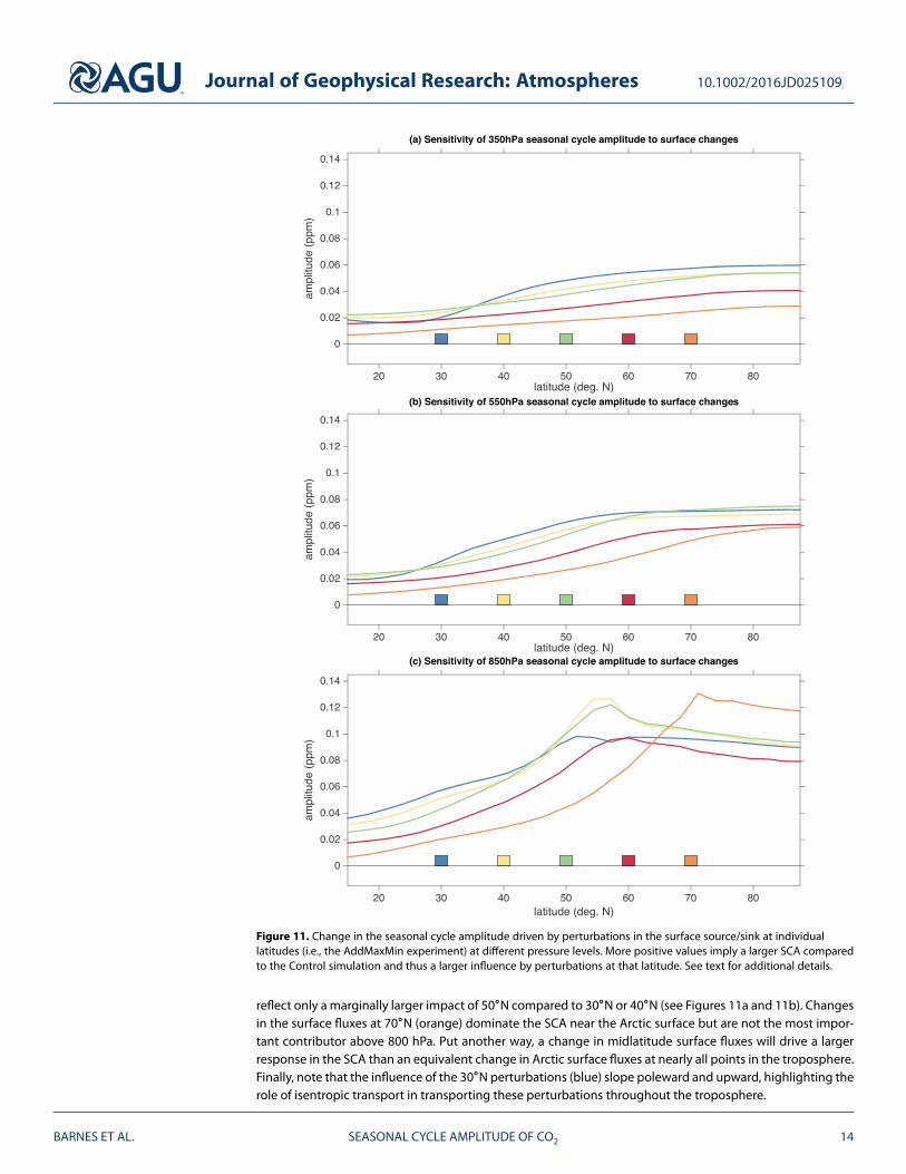
The resulting changes in the SCA at 350 hPa, 550 hPa, and 850 hPa are plotted in Figure 11. The five coloredlines correspond to the amplitude change for the five different simulations where the fluxes at five differentlatitudes (colored rectangles) were perturbed. SCA changes for all perturbations at all latitudes are positive inFigure 11 indicating that increasing the seasonal cycle of the emissions increases the SCA of the tracer every-where. However, the differences between the five simulations indicate that changes in the surface emissionsat some latitudes are more important than changes at other latitudes. Specifically, in the upper (350 hPa)and middle troposphere (550 hPa)(Figures 11a and 11b), emission changes at 30∘N (blue) and 50∘N (green)dominate the changes in SCA at most northern latitudes, including the Arctic. Even near the surface at 70∘N(the latitude of Barrow, Alaska; Figure 11c), the tracer SCA is more sensitive to an increase in seasonal fluxesat 30∘N (blue) than 60∘N (red).

To quantify the relative importance of these perturbations throughout the entire troposphere, we plot inFigure 12 the latitude perturbation which results in the largest change in SCA. Perturbations at 30∘N (blue)and 50∘N (green) have the largest impact on the SCA at nearly all locations, with perturbations at 40∘N(yellow) and 60∘N (red) making prominent contributions at select locations. We caution that the dominanceof flux changes at 50∘N in the subtropical middle to upper troposphere should not be overinterpreted, as they



Figure 11. Change in the seasonal cycle amplitude driven by perturbations in the surface source/sink at individuallatitudes (i.e., the AddMaxMin experiment) at different pressure levels. More positive values imply a larger SCA comparedto the Control simulation and thus a larger influence by perturbations at that latitude. See text for additional details.

reflect only a marginally larger impact of 50∘N compared to 30∘N or 40∘N (see Figures 11a and 11b). Changesin the surface fluxes at 70∘N (orange) dominate the SCA near the Arctic surface but are not the most impor-tant contributor above 800 hPa. Put another way, a change in midlatitude surface fluxes will drive a largerresponse in the SCA than an equivalent change in Arctic surface fluxes at nearly all points in the troposphere.Finally, note that the influence of the 30∘N perturbations (blue) slope poleward and upward, highlighting therole of isentropic transport in transporting these perturbations throughout the troposphere.



Figure 12. The latitude that most increases the seasonal cycle amplitude at each latitude/pressure point when thesurface source/sink is perturbed in the months with the maximum and minimum source and sink, respectively. See textfor additional details. Black lines denote the March isentropes.

The experimental design of the AddMaxMin simulations takes into account the larger area at lower latitudescompared to higher latitudes by defining the perturbation in terms of flux per meter squared. However, in theNorthern Hemisphere, land is not distributed equally across latitude bands, but rather, the fraction of land athigh latitudes is larger than the fraction at lower latitudes. Taking the fractional area that is land into account(using values Hartmann [1994, Figure 1-12]) leads to similar conclusions as found in Figure 12, except thatcontributions from 50∘N dominate the tropospheric sensitivity, and the dominating influence of emissionschanges at 70∘N is felt at slightly higher altitudes (i.e., up to 650 hPa; not shown).

The results of this section can be summarized by two main conclusions. (1) The majority of the seasonal cycleamplitude of CO2 at high latitudes is driven by fluxes outside of the Arctic (e.g., Figure 9 and Figure 10).(2) The seasonal cycle amplitude is most sensitive to changes in the seasonality of midlatitude surface emis-sions throughout most of the troposphere. Only near the Arctic surface are changes in emissions at the Arcticsurface the dominant driver (e.g., Figure 12), although it contributes only 20% more than the flux changes atlower latitudes (Figure 11c) in the idealized model.

Drivers of the near-surface Arctic SCA are especially important since the majority of high-latitude CO2 mea-surements are taken at or near the surface. Results from the idealized model suggest that near the surface,Arctic fluxes and midlatitude fluxes are both important contributors to the SCA there. We expect that if any-thing, the idealized model underestimates the influence of midlatitude fluxes on the SCA near the Arcticsurface since the Arctic surface does not get cold enough in the idealized model, and thus, the diabatic cool-ing (and cross-isentropic sinking) is likely too weak. This sinking at high latitudes transports midlevel tracer(transported from lower latitudes) down, and thus, weaker sinking implies a weaker signature of lower lati-tude fluxes at the Arctic surface. Evidence of this can be seen in Figure 7, where the Arctic isentropes havesteeper slopes in the idealized model compared to GEOS-Chem. Furthermore, comparing the ArcticOff exper-iments between the two models (Figure 10) shows that the idealized model suggests a smaller role for Arcticfluxes in driving near-surface SCA (35%; blue lines in Figure 10b) compared to the idealized model (40%; bluelines in Figure 10a).

3.4. Circulation-Driven SeasonalityUp until now, we have discussed the seasonality of the idealized tracer as a whole. However, this seasonality isactually driven by two separate components: (1) a seasonality in the tracer source/sink and (2) a seasonality inthe atmospheric transport (i.e., circulation). In order to investigate the relative roles of each of these two com-ponents, we make use of our idealized modeling framework and discuss simulations where the seasonality of



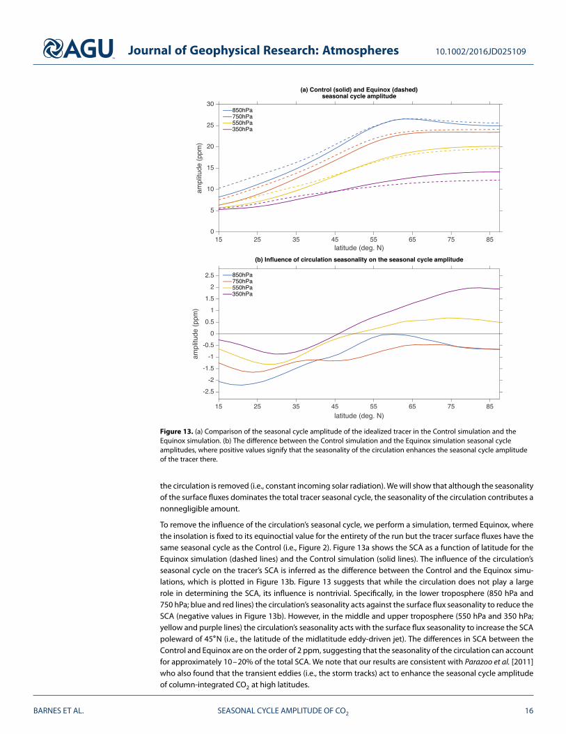
Figure 13. (a) Comparison of the seasonal cycle amplitude of the idealized tracer in the Control simulation and theEquinox simulation. (b) The difference between the Control simulation and the Equinox simulation seasonal cycleamplitudes, where positive values signify that the seasonality of the circulation enhances the seasonal cycle amplitudeof the tracer there.

the circulation is removed (i.e., constant incoming solar radiation). We will show that although the seasonalityof the surface fluxes dominates the total tracer seasonal cycle, the seasonality of the circulation contributes anonnegligible amount.

To remove the influence of the circulation’s seasonal cycle, we perform a simulation, termed Equinox, wherethe insolation is fixed to its equinoctial value for the entirety of the run but the tracer surface fluxes have thesame seasonal cycle as the Control (i.e., Figure 2). Figure 13a shows the SCA as a function of latitude for theEquinox simulation (dashed lines) and the Control simulation (solid lines). The influence of the circulation’sseasonal cycle on the tracer’s SCA is inferred as the difference between the Control and the Equinox simu-lations, which is plotted in Figure 13b. Figure 13 suggests that while the circulation does not play a largerole in determining the SCA, its influence is nontrivial. Specifically, in the lower troposphere (850 hPa and750 hPa; blue and red lines) the circulation’s seasonality acts against the surface flux seasonality to reduce theSCA (negative values in Figure 13b). However, in the middle and upper troposphere (550 hPa and 350 hPa;yellow and purple lines) the circulation’s seasonality acts with the surface flux seasonality to increase the SCApoleward of 45∘N (i.e., the latitude of the midlatitude eddy-driven jet). The differences in SCA between theControl and Equinox are on the order of 2 ppm, suggesting that the seasonality of the circulation can accountfor approximately 10–20% of the total SCA. We note that our results are consistent with Parazoo et al. [2011]who also found that the transient eddies (i.e., the storm tracks) act to enhance the seasonal cycle amplitudeof column-integrated CO2 at high latitudes.



4. Discussion and Conclusions

The results of this study can be summarized by two main conclusions.

1. The seasonal cycle amplitude of CO2 roughly follows surfaces of constant potential temperature, ratherthan pressure surfaces. Thus, isentropic transport is the fundamental reason for the latitudinal gradient ofincreasing CO2 seasonal cycle amplitude along pressure surfaces throughout the troposphere, given thepresent-day latitudinal distribution of CO2 emissions.

2. Since changes in the seasonal cycle amplitude follow surfaces of constant potential temperature, increasingseasonal fluxes in lower latitudes (i.e., temperate and boreal regions) have a larger impact on the seasonalcycle amplitude of CO2 throughout most of the troposphere compared to increasing seasonal fluxes inhigher latitudes (i.e., Arctic region). That is, amplification of surface flux seasonality at 30∘N has a biggereffect than an equivalent amplification at 60∘N when observed at 70∘N, where SCA has been observed sincethe early 1960s at Barrow, Alaska.

In support of a dominant role of isentropic transport in carrying the seasonal cycle amplitude from themidlatitude surface to the Arctic, we find that the seasonal cycle amplitude of CO2 increases with latitude inde-pendent of Arctic surface fluxes. Specifically, transport from lower latitudes accounts for approximately 60% ofthe northern high-latitude seasonal cycle even in the presence of a strongly seasonal Arctic biosphere. Theseresults support the hypothesis that recently observed increasing CO2 seasonal cycle amplitude at the surfaceand throughout the middle troposphere in northern high latitudes [e.g., Graven et al., 2013; Forkel et al., 2016;Zeng et al., 2014] is likely driven by changes in midlatitude surface fluxes (i.e., temperature ecosystems), ratherthan changes in the Arctic. Our results demonstrate the critical importance of advective fluxes from muchlower latitudes in controlling seasonal variations of CO2 over Boreal and Arctic latitudes, especially aloft.Regional inverse models must include accurate specification of meridional transport by individual synopticevents as lateral boundary conditions [Chang et al., 2014; Henderson et al., 2015; Karion et al., 2015].

The above conclusions are supported by tracer experiments in an idealized aquaplanet with no topographybut are also reproduced by experiments with GEOS-Chem which includes topography and where transportis driven by reanalysis winds. Agreement between these two very different models points to a fundamentalrelationship between the periodic surface fluxes of any tracer and its high-latitude concentrations. That sucha simplified aquaplanet can reproduce the observed latitudinal gradient in the seasonal cycle amplitude ofCO2 along pressure surfaces suggests that transport by synoptic eddies alone can account for this behavior.

It is well known that the distribution of atmospheric trace gases is strongly influenced by convective activ-ity [Denning et al., 1996], especially along the midlatitude storm tracks where vertical mixing is significantlyenhanced by synoptic eddies and moist convective processes [Miyazaki et al., 2008; Parazoo et al., 2011, 2012].Quantitative estimation of surface fluxes using modern atmospheric transport models includes these trans-port processes, but meridional transport in synoptic weather systems includes fine-scale mechanisms likefrontal lifting and vertical motion in clouds that are unresolved by global models. Cloud permitting climatemodels produce more realistic vertical gradients of passive tracers compared to models utilizing conventionalconvective parameterizations [e.g., Rosa et al., 2012] and drive enhanced poleward transport of trace gasesfrom midlatitude source regions [Wang et al., 2011]. Thus, it is likely that the estimates in this study, whichare derived from two models that do not explicitly resolve convective processes, underestimate the influ-ence of isentropic transport and hence the seasonal cycle amplitude of CO2 in the midtroposphere. Futurework should consider the effect of resolved convection, with careful analysis of transport on dry versus moistisentropic surfaces.

Appendix A

The gray-radiation aquaplanet of Frierson et al. [2006] does not include a seasonal cycle by default and istypically run under equinoctial conditions. Thus, here we will briefly describe how a 360 day seasonal cycle wassimulated. First, the model computes the top-of-atmosphere average daily insolation according to the formulaprovided in equation (2.17) of Hartmann [1994]. However, the resulting seasonal cycle of the circulation isvery unrealistic, with much too strong of a seasonality, e.g., the summer time jet stream and storm track liepoleward of 60∘N. To make the seasonal cycle more realistic, we modify the default parameters of Friersonet al. [2006] and follow Afargan and Kaspi [2016] by defining a top-of-atmosphere (TOA) albedo:

𝛼TOA = 𝛼TOA0+(𝛼TOA1

− 𝛼TOA0

)⋅ sin(𝜃)4, (A1)



where 𝜃 is degrees latitude, where 𝛼TOA0= 0.05 and 𝛼TOA1

= 0.45. Then, the net downward solar radiationis multiplied by (1 − 𝛼TOA) to partially mute the default seasonal cycle. Finally, the surface longwave atmo-spheric optical depths at equator and pole (which approximate the effects of water vapor) [Frierson et al., 2006,equation (4)] are modified to be 𝜏0e = 16.0 and 𝜏0p = 8.0. We note that while these modifications to thedefault parameters result in a more realistic seasonal cycle of the circulation, the general conclusions of thiswork would remain the same if the default parameters were used instead.

ReferencesAfargan, H., and Y. Kaspi (2016), A Midwinter Minimum in Storm Track Activity in an Idealized GCM With a Seasonal Cycle, EGU General

Assembly, Vienna, Austria.Arora, V. K., et al. (2013), Carbon–concentration and carbon–climate feedbacks in CMIP5 Earth system models, J. Clim., 26(15), 5289–5314.Bacastow, R., and C. Keeling (1981), Atmospheric carbon dioxide concentration and the observed airborne fraction, Carbon cycle Model.,

SCOPE, 16, 103–112.Bakwin, P., K. Davis, C. Yi, S. Wofsy, J. Munger, L. Haszpra, and Z. Barcza (2004), Regional carbon dioxide fluxes from mixing ratio data, Tellus

Ser. B, 56(4), 301–311.Barth, M., et al. (2007), Cloud-scale model intercomparison of chemical constituent transport in deep convection, Atmos. Chem. Phys., 7(18),

4709–4731.Bey, I., D. J. Jacob, R. M. Yantosca, J. A. Logan, B. Field, A. M. Fiore, Q. Li, H. Liu, L. J. Mickley, and M. Schultz (2001), Global modeling of

tropospheric chemistry with assimilated meteorology: Model description and evaluation, J. Geophys. Res., 106(114), 23,073–23,096.Chang, R. Y.-W., et al. (2014), Methane emissions from alaska in 2012 from carve airborne observations, Proc. Natl. Acad. Sci., 111(47),

16,694–16,699.Corbin, K., A. Denning, and N. Parazoo (2009), Assessing temporal clear-sky errors in assimilation of satellite CO2 retrievals using a global

transport model, Atmos. Chem. Phys., 9(9), 3043–3048.Cox, P. M., R. Betts, M. Collins, P. Harris, C. Huntingford, and C. Jones (2004), Amazonian forest dieback under climate-carbon cycle

projections for the 21st century, Theor. Appl. Climatol., 78(1–3), 137–156.Cramer, W., et al. (2001), Global response of terrestrial ecosystem structure and function to CO2 and climate change: Results from six

dynamic global vegetation models, Global Change Biol., 7(4), 357–373.Crawford, J., et al. (2003), Clouds and trace gas distributions during TRACE-P, J. Geophys. Res., 108(21), 8818, doi:10.1029/2002JD003177.Denning, A. S., D. A. Randall, G. J. Collatz, and P. J. Sellers (1996), Simulations of terrestrial carbon metabolism and atmospheric CO2 in a

general circulation model. Part 2: Simulated CO2 concentrations, Tellus Ser. B, 48(4), 542–567.Dlugokencky, E., K. Masarie, P. Lang, and P. Tans (2015), NOAA Greenhouse Gas Reference from Atmospheric Carbon Dioxide

Dry Air Mole Fractions from the NOAA ESRL Carbon Cycle Cooperative Global Air Sampling Network. [Available atftp://aftp.cmdl.noaa.gov/data/trace_gases/co2/flask/surface/.]

Fisher, J. B., et al. (2014a), Carbon cycle uncertainty in the Alaskan Arctic, Biogeosciences, 11, 4271–4288.Fisher, J. B., D. N. Huntzinger, C. R. Schwalm, and S. Sitch (2014b), Modeling the terrestrial biosphere, Annu. Rev. Environ. Resour., 39, 91–123.Forkel, M., N. Carvalhais, C. Rödenbeck, R. Keeling, M. Heimann, K. Thonicke, S. Zaehle, and M. Reichstein (2016), Enhanced seasonal CO2

exchange caused by amplified plant productivity in northern ecosystems, Science, 4971, 1–9, doi:10.1126/science.aac4971.Frierson, D. M. W., I. M. Held, and P. Zurita-Gator (2006), A gray-radiation aquaplanet moist GCM: Static stability and eddy scale, J. Atmos. Sci.,

63, 2548–2566.Fung, I., K. Prentice, E. Matthews, J. Lerner, and G. Russell (1983), Three-dimensional tracer model study of atmospheric CO2: Response to

seasonal exchanges with the terrestrial biosphere, J. Geophys. Res., 88(C2), 1281–1294.Fung, I., C. Tucker, and K. Prentice (1987), Application of advanced very high resolution radiometer vegetation index to study

atmosphere-biosphere exchange of CO2, J. Geophys. Res., 92(D3), 2999–3015.Graven, H. D., et al. (2013), Enhanced seasonal exchange of CO2 by Northern Ecosystems since 1960, Science, 341(6150), 1085–1089,

doi:10.1126/science.1239207.Gray, J. M., S. Frolking, E. A. Kort, D. K. Ray, C. J. Kucharik, N. Ramankutty, and M. A. Friedl (2014), Direct human influence on atmospheric

CO2 seasonality from increased cropland productivity, Nature, 515(7527), 398–401.Gregory, J. M., C. Jones, P. Cadule, and P. Friedlingstein (2009), Quantifying carbon cycle feedbacks, J. Clim., 22(19), 5232–5250.Harris, I., P. D. Jones, T. J. Osborn, and D. H. Lister (2014), Updated high-resolution grids of monthly climatic observations—The CRU TS3.10

Dataset, Int. J. Climatol., 34(3), 623–642, doi:10.1002/joc.3711.Hartmann, D. L. (1994), Global Physical Climatology, vol. 56, 411 pp., Academic Press, San Diego, Calif.Helliker, B. R., J. A. Berry, A. K. Betts, P. S. Bakwin, K. J. Davis, A. S. Denning, J. R. Ehleringer, J. B. Miller, M. P. Butler, and D. M. Ricciuto (2004),

Estimates of net CO2 flux by application of equilibrium boundary layer concepts to CO2 and water vapor measurements from a talltower, J. Geophys. Res., 109(D20), D20106, doi:10.1029/2004JD004532.

Henderson, J., et al. (2015), Atmospheric transport simulations in support of the Carbon in Arctic Reservoirs Vulnerability Experiment(CARVE), Atmos. Chem. Phys., 15(8), 4093–4116.

Hoffman, F., et al. (2014), Causes and implications of persistent atmospheric carbon dioxide biases in Earth system models, J. Geophys. Res.Biogeosci., 119, 141–162, doi:10.1002/2013JG002381.

Hopkins, F. M., M. S. Torn, and S. E. Trumbore (2012), Warming accelerates decomposition of decades-old carbon in forest soils, Proc. Natl.Acad. Sci., 109(26), E1753—E1761.

Huntzinger, D. N., et al. (2013), The north american carbon program multi-scale synthesis and terrestrial model intercomparisonproject—Part 1: Overview and experimental design, Geosci. Model Dev., 6(6), 2121–2133.

Hurwitz, M. D., D. M. Ricciuto, P. S. Bakwin, K. J. Davis, W. Wang, C. Yi, and M. P. Butler (2004), Transport of carbon dioxide in the presence ofstorm systems over a Northern Wisconsin forest, J. Atmos. Sci., 61(5), 607–618.

Kalnay, E., et al. (1996), The NCEP/NCAR 40-year reanalysis project, Bull. Am. Meteorol. Soc., 83, 437–471.Karion, A., et al. (2015), Investigating alaskan methane and carbon dioxide fluxes using measurements from the CARVE tower, Atmos. Chem.

Phys. Discuss., 15(23), 34,871–34,911.Keeling, C. D. (1960), The concentration and isotopic abundances of carbon dioxide in the atmosphere, Tellus, 12(2), 200–203.Keppel-Aleks, G., P. O. Wennberg, and T. Schneider (2011), Sources of variations in total column carbon dioxide, Atmos. Chem. Phys., 11(8),

3581–3593, doi:10.5194/acp-11-3581-2011.

AcknowledgmentsThe authors would like to thank threeanonymous reviewers for their helpfulcomments on an earlier version of thismanuscript. E.A.B. was supported bythe Climate and Large-scale DynamicsProgram of the National ScienceFoundation under grant 1419818.A.S.D. gratefully acknowledgessupport from NASA’s ScienceMission Directorate under theAtmospheric Carbon Transport project(NNX15AJ09G). Part of the researchin this study was performed at theJet Propulsion Laboratory, CaliforniaInstitute of Technology, undercontract with the National Aeronauticsand Space Administration. We thankC. Koven for providing CLM4.5 CO2surface flux fields, and the ODIACfossil fuel CO2 emissions wereprovided by T. Oda. The modeloutput supporting the conclusionsof this article is available from thecorresponding author upon request([email protected]).


http://dx.doi.org/10.1029/2002JD003177

ftp://aftp.cmdl.noaa.gov/data/trace_gases/co2/flask/surface/

http://dx.doi.org/10.1126/science.aac4971

http://dx.doi.org/10.1126/science.1239207

http://dx.doi.org/10.1002/joc.3711

http://dx.doi.org/10.1029/2004JD004532

http://dx.doi.org/10.1002/2013JG002381

http://dx.doi.org/10.5194/acp-11-3581-2011

mailto:[email protected]


Keppel-Aleks, G., et al. (2012), The imprint of surface fluxes and transport on variations in total column carbon dioxide, Biogeosciences, 9(3),875–891, doi:10.5194/bg-9-875-2012.

Klonecki, A., P. Hess, L. Emmons, L. Smith, J. Orlando, and D. Blake (2003), Seasonal changes in the transport of pollutants into the Arctictroposphere-model study, J. Geophys. Res., 108(D4), 8367, doi:10.1029/2002JD002199.

Lagenhorst, A. (2005), Spectral Atmospheric Core Documentation, Tech. Rep., Geophysical Fluid Dynamics Laboratory, Princeton, N. J.Le Quéré, C., et al. (2015), Global carbon budget 2014, Earth Syst. Sci. Data, 7, 47–85.LeBauer, D. S., and K. K. Treseder (2008), Nitrogen limitation of net primary productivity in terrestrial ecosystems is globally distributed,

Ecology, 89, 371–379.Lin, S., and R. Rood (1996), Multidimensional flux-form semi-Lagrangian transport schemes, Mon. Weather Rev., 124, 2046–2070,

doi:10.1175/1520-0493.Luo, Y., D. Hui, and D. Zhang (2006), Elevated CO2 stimulates net accumulations of carbon and nitrogen in land ecosystems: A meta-analysis,

Ecology, 87(1), 53–63.Messerschmidt, J., N. Parazoo, D. Wunch, N. M. Deutscher, C. Roehl, T. Warneke, and P. O. Wennberg (2013), Evaluation of seasonal

atmosphere-biosphere exchange estimations with TCCON measurements, Atmos. Chem. Phys., 13(10), 5103–5115,doi:10.5194/acp-13-5103-2013.

Miller, C. E., and S. J. Dinardo (2012), Carve: The Carbon in Arctic Reservoirs Vulnerability Experiment, in IEEE Aerospace Conference,pp. 1–17, IEEE, Big Sky, Mont., doi:10.1109/AERO.2012.6187026.

Miyazaki, K., P. Patra, M. Takigawa, T. Iwasaki, and T. Nakazawa (2008), Global-scale transport of carbon dioxide in the troposphere,J. Geophys. Res., 113, doi:10.1029/2007JD009557.

Nassar, R., et al. (2010), Modeling global atmospheric co2 with improved emission inventories and co2 production from the oxidation ofother carbon species, Geosci. Model Dev., 3(2), 689–716, doi:10.5194/gmd-3-689-2010.

Oda, T., and S. Maksyutov (2011), A very high-resolution (1 km × 1 km) global fossil fuel CO2 emission inventory derived using a pointsource database and satellite observations of nighttime lights, Atmos. Chem. Phys., 11, 543–556.

Oleson, K. W., et al. (2013), Technical description of version 4.5 of the Community Land Model (CLM), Tech. Rep. NCAR/TN-503+STR, NCAR,doi:10.5065/D6RR1W7M.

Orbe, C., M. Holzer, L. M. Polvani, and D. Waugh (2013), Air-mass origin as a diagnostic of tropospheric transport, J. Geophys. Res. Atmos., 118,1459–1470, doi:10.1002/jgrd.50133.

Parazoo, N., A. Denning, S. Kawa, K. Corbin, R. Lokupitiya, and I. Baker (2008), Mechanisms for synoptic variations of atmospheric CO2 inNorth America, South America and Europe, Atmos. Chem. Phys., 8(23), 7239–7254.

Parazoo, N. C., A. S. Denning, J. A. Berry, A. Wolf, D. A. Randall, S. R. Kawa, O. Pauluis, and S. C. Doney (2011), Moist synoptic transport of CO2along the mid-latitude storm track, Geophys. Res. Lett., 38, L09804, doi:10.1029/2011GL047238.

Parazoo, N. C., A. S. Denning, S. R. Kawa, S. Pawson, and R. Lokupitiya (2012), CO2 flux estimation errors associated with moist atmosphericprocesses, Atmos. Chem. Phys., 12(14), 6405–6416, doi:10.5194/acp-12-6405-2012.

Parazoo, N. C., et al. (2013), Interpreting seasonal changes in the carbon balance of southern Amazonia using measurements of XCO2 andchlorophyll fluorescence from GOSAT, Geophys. Res. Lett., 40, 2829–2833, doi:10.1002/grl.50452.

Parazoo, N. C., R. Commane, S. Wofsy, C. Koven, C. Sweeney, D. Lawrence, J. Lindaas, R. Y.-W. Chang, and C. E. Miller (2016), Detectingpatterns of changing CO2 flux in Alaska, Proc. Natl. Acad. Sci. U.S.A., doi:10.1073/pnas.1601085113.

Pauluis, O., A. Czaja, and R. Korty (2010), The global atmospheric circulation in moist isentropic coordinates, J. Clim., 23(11), 3077–3093.Pearman, G., and P. Hyson (1980), Activities of the global biosphere as reflected in atmospheric CO2 records, J. Geophys. Res. Oceans, 85(C8),

4457–4467.Randerson, J. T., M. V. Thompson, T. J. Conway, I. Y. Fung, and C. B. Field (1997), The contribution of terrestrial sources and sinks to trends in

the seasonal cycle of atmospheric carbon dioxide, Global Biogeochem. Cycles, 11(4), 535–560.Rosa, D., J. F. Lamarque, and W. D. Collins (2012), Global transport of passive tracers in conventional and superparameterized climate

models: Evaluation of multi-scale methods, J. Adv. Model. Earth Systems, 4(10), M10003, doi:10.1029/2012MS000206.Schuur, E., et al. (2013), Expert assessment of vulnerability of permafrost carbon to climate change, Clim. Change, 119(2), 359–374,

doi:10.1007/s10584-013-0730-7.Shevliakova, E., S. W. Pacala, S. Malyshev, G. C. Hurtt, P. Milly, J. P. Caspersen, L. T. Sentman, J. P. Fisk, C. Wirth, and C. Crevoisier (2009),

Carbon cycling under 300 years of land use change: Importance of the secondary vegetation sink, Global Biogeochem. Cycles, 23,GB2022, doi:10.1029/2007GB003176.

Stohl, A. (2006), Characteristics of atmospheric transport into the Arctic troposphere, J. Geophys. Res., 111, D11306,doi:10.1029/2005JD006888.

Takahashi, T., et al. (2009), Climatological mean and decadal change in surface ocean pCO2, and net sea-air CO2 flux over the global oceans,Deep Sea Res. Part II, 56(8-10), 554–577, doi:10.1016/j.dsr2.2008.12.009.

Tian, H., et al. (2015), Global patterns and controls of soil organic carbon dynamics as simulated by multiple terrestrial biosphere models:Current status and future directions, Global Biogeochem. Cycles, 29, 775–792, doi:10.1002/2014GB005021.

Wang, M., S. Ghan, M. Ovchinnikov, X. Liu, R. Easter, E. Kassianov, Y. Qian, and H. Morrison (2011), Aerosol indirect effects in a multi-scaleaerosol-climate model PNNL-MMF, Atmos. Chem. Phys., 11( 11), 5431–5455, doi:10.5194/acp-11-5431-2011.

Wenzel, S., P. M. Cox, V. Eyring, and P. Friedlingstein (2014), Emergent constraints on climate-carbon cycle feedbacks in the CMIP5 Earthsystem models, J. Geophys. Res. Biogeosci., 119, 794–807, doi:10.1002/2013JG002591.

Wunch, D., et al. (2013), The covariation of Northern Hemisphere summertime CO2 with surface temperature in boreal regions, Atmos.Chem. Phys., 13(18), 9447–9459, doi:10.5194/acp-13-9447-2013.

Zeng, N., F. Zhao, G. J. Collatz, E. Kalnay, R. J. Salawitch, T. O. West, and L. Guanter (2014), Agricultural Green Revolution as a driver ofincreasing atmospheric CO2 seasonal amplitude, Nature, 515(7527), 394–397, doi:10.1038/nature13893.


http://dx.doi.org/10.5194/bg-9-875-2012

http://dx.doi.org/10.1029/2002JD002199

http://dx.doi.org/10.1175/1520-0493


http://dx.doi.org/10.1109/AERO.2012.6187026

http://dx.doi.org/10.1029/2007JD009557

http://dx.doi.org/10.5194/gmd-3-689-2010

http://dx.doi.org/10.5065/D6RR1W7M

http://dx.doi.org/10.1002/jgrd.50133

http://dx.doi.org/10.1029/2011GL047238


http://dx.doi.org/10.1002/grl.50452

http://dx.doi.org/10.1073/pnas.1601085113

http://dx.doi.org/10.1029/2012MS000206

http://dx.doi.org/10.1007/s10584-013-0730-7

http://dx.doi.org/10.1029/2007GB003176

http://dx.doi.org/10.1029/2005JD006888

http://dx.doi.org/10.1016/j.dsr2.2008.12.009

http://dx.doi.org/10.1002/2014GB005021


http://dx.doi.org/10.1002/2013JG002591


http://dx.doi.org/10.1038/nature13893

Isentropic transport and the seasonal cycle amplitude of CO2

Documents

Transcript of Isentropic transport and the seasonal cycle amplitude of CO2