Electronic copy available at: http://ssrn.com/abstract=1270606

Is the “curse of natural resources” really a curse?

March 20, 2008

ERID Working Paper Number 14

This paper can be downloaded without charge from

The Social Science Research Network Electronic Paper Collection: http://ssrn.com/abstract=1270606

Pietro Peretto

Duke University

Electronic copy available at: http://ssrn.com/abstract=1270606

Is the “curse of natural resources” really a curse?

Pietro F. Peretto∗

Department of EconomicsDuke University

March 20, 2008

Abstract

This paper takes a new look at the long-run implications of re-source abundance. Using a Schumpeterian growth model that yieldsan analyitical solution for the transition path, it derives conditionsunder which the “curse of natural resources” occurs and is in fact acurse, meaning that welfare falls, conditions under which it occurs butit is not a curse, meaning that growth slows down but welfare risesnevertheless, and conditions under which it does not occur at all. Aneffective way to summarize the results is to picture growth and wel-fare as hump-shaped functions of resource abundance. The propertythat the peak of growth occurs earlier than the peak of welfare cap-tures the crucial role of initial consumption, which rises with resourceabundance, and is an important reminder that the welfare effect of re-source abundance depends on the whole path of consumption, not ona summary statistic of its slope. Growth regressions that ignore theendogeneity of initial income do not provide sufficient information toassess whether resource abundance is bad even if one could prove be-yond reasonable doubt that the relation is indeed negative and causal.Recent evidence that the correlation is actually positive should makeus even more skeptical of policy advice based on the “curse” logic.

Keywords: Endogenous Growth, Endogenous Technological Change,Curse of Natural Resources.JEL Classification Numbers: E10, L16, O31, O40

∗Address: Department of Economics, Duke University, Durham, NC 27708. Phone:(919) 6601807. Fax: (919) 6848974. E-mail: peretto@econ.duke.edu. The idea for thispaper was conceived during stimulating discussions with several members of the EconomicsDepartment at the University of Calgary, in particular Sjak Smulders and Francisco Gon-zales. Thanks to all for the hospitality and the comments.

1

Electronic copy available at: http://ssrn.com/abstract=1270606

1 Introduction

The debate on the role that natural resources play in the long-run fortunesof the economy is as lively as ever. Currently it focuses on the influentialwork of Sachs and Warner (1995, 2001), who find a negative cross-countrycorrelation between the share of natural resources exports in GDP and thegrowth rate of GDP per capita, and interpret the export share as a measureof natural resource abundance. This finding poses tough questions for eco-nomic theory and policy – the idea that abundant resources are bad for theeconomy strikes many as a paradox. Not surprisingly, then, it has spurreda large amount of work that has added to an already large literature.1

Roughly speaking, the current debate pitches explanations of the neg-ative correlation based on institutional deterioration, whereby natural re-sources create the opportunity for rent-seeking, corruption and conflict,against explanations based on sectoral reallocation, whereby activities in-tensive in natural resources crowd out other, more technologically dynamicactivities (e.g., manufacturing, knowledge-based services).2 Recently, some-thing akin to a third side has emerged as some researchers find a positivecorrelation between growth and resource abundance and conclude that thereis no paradox to resolve.3

The motivation for this paper is what all sides of the debate have incommon. Empirical contributions take as given that the slower growth as-sociated to resource abundance is bad – hence referring to it as the “curseof natural resources” is accepted practice – and that dispelling the “curse”requires proving that the correlation is, in fact, positive; theoretical contri-butions discuss specific mechanisms producing slower growth, not whetherslower growth yields lower welfare. Underlying this literature, thus, seemsto be the tacit assumption growth = welfare.

This is puzzling since the notion that growth and welfare are not thesame is the cornerstone of the intertemporal trade-off at the heart of modern

1A comprehensive review is beyond the scope of the paper. The interested reader canconsult Gylfason (2001a), Stevens (2003) or Lederman and Maloney (2007).

2From this viewpoint, of particular interest is the evidence in Papyrakis and Gerlagh(2007) and Boyce and Emery (2007), who document a negative correlation across U.S.states between the growth rate of the Gross State Product (GSP) and, respectively, theshare of the primary sector in GSP and the share of employment in mining. Because theyfocus on U.S. states, these studies raise important issues for institution-based stories.

3The positive correlation is actually not new; see Sala-i-Martin (1997), Sala-i-Martin,Doppelhofer and Miller (2004). What is new is the explicit assertion that the “curse” doesnot exist; see Alexeev and Conrad (2007), Brunneschweiler and Bulte (2007), Ledermanand Maloney (2007b).

2

growth theory. Moreover, since the correlation between resource abundanceand the initial level of GDP per capita is positive it is not at all obvious thatresource abundant countries are worse off.4 Similarly puzzling is that empir-ical papers only rarely state explicitly whether “curse” denotes a permanentor a temporary slowdown. Yet, such a property is surely of consequence forthe welfare effects that we can expect. If the slowdown is permanent, it caneasily dominate the level effect of resources abundance; if it is temporary,it can be dominated by the level effect. It follows that the specifics of thegrowth model that one uses to interpret the regressions are of paramountimportance and should be discussed explicitly.5

4See Rodriguez and Sachs (1999), Bravo-Ortega and De Gregorio (2007) and, expe-cially, Alexeev and Conrad (2007) for cross-country evidence; see also Boyce and Emery(2007) for U.S. states

5 It is worth discussing examples of papers that tackle these issues to some extent toillustrate what I have in mind. Bravo-Ortega and de Gregorio (2007) develop a theoreticalmodel whose predictions they take to the data. However, they don’t use the model todraw welfare implications – surprisingly so, since they emphasize the positive relationbetween resource abundance and the whole path of log-income (see Figure 4.1, p. 80)and thus forewarn the reader that not only the intertemporal trade-off plays a crucialrole in interpreting the regressions, but that the predicted welfare effect is positive. Themost striking example of this practice is Rodriguez and Sachs (1999), who develop a fullyspecified simulation model of the Venezuelan economy and document that that country’sgrowth experience is due to the fact that the discovery of oil allows it to live beyond itsmeans – meaning that it converges to the steady state from above. Despite having all theingredients, they do not calculate the discounted integral of utility to show that such a pathis in fact associated to lower welfare; they only remark in the conclusions that experiencingfalling income and consumption is bad. It surely is, but it is not clear that looking at flowutility answers the key question: Would Venezuela be better off if it hadn’t found oil?After all, it converges from above because it overshoots the steady state in the first place.To argue that the slower growth subsequent to the inital overshooting period produceslower welfare, at a minimum they need to argue that the economy converges to a lowersteady state (convergence from above to the same steady state, as it seems to be the casein the data reported in Figure 3, p. 289, yields higher welfare). Among purely empiricalpapers, Gylfason (2001b) documents the negative relation between growth and the shareof natural wealth in national wealth and then writes: “Shaving one percentage point ofany country’s annual growth rate is a serious matter because the (weighted) average rateof per capita growth in the world economy since 1965 has been about 1.5 percent peryear” (p. 849). Thus, the benchmark for infering that a high share of natural wealth is abad thing is the world’s average growth rate, not the economy’s own welfare. Papyrakisand Gerlagh (2003, 2007) derive the long-run income effect of resource abundance fromthe transition dynamics of the standard reduced-form, log-linear representation of growthmodels. However, they are never explicit about (i) how resource abundance affects steady-state growth and initial income and (ii) how the long-run income effect that they computerelates to welfare. Welfare usually depends on the whole path of consumption (as inthe papers just discussed) and the long-run income effect alone is not sufficient to assesswhether it rises or falls with resource abundance. The paper that is most explicit about

3

In this paper I take to heart these observations and take a new look atthe long-run implications of resource abundance through the lens of modernSchumpeterian growth theory. In particular, I use a model of the latest vin-tage that allows me to study welfare analytically. I derive conditions underwhich the “curse” occurs and is in fact a curse, meaning that welfare falls,conditions under which it occurs but it is not a curse, meaning that growthslows down but welfare rises nevertheless, and conditions under which itdoes not occur at all.

The model has two factors of production in exogenous supply, labor anda natural resource, and two sectors, primary production (or resource process-ing) and manufacturing. I define resource abundance as the endowment ofthe natural resource relative to labor. The primary sector uses labor toprocess the raw natural resource; the manufacturing sector uses labor andthe processed natural resource to produce differentiated consumption goods.Because both sectors use labor, its reallocation from manufacturing to pri-mary production drives the economy’s adjustment to an increase in resourceabundance. The manufacturing sector is technologically dynamic: firms andentrepreneurs undertake R&D to learn how to use factors of production moreefficiently and to design new products. Importantly, the process of productproliferation fragments the aggregate market into submarkets whose sizedoes not increase with the size of the endowments and thereby sterilizes thescale effect. This means that the effect of resource abundance on growth isonly temporary. The resulting structure is extremely tractable and yields aclosed-form solution for the transition path.

The core mechanism is how the pattern of factor substitution in the twosectors determines the response of the natural resource price to an increasein the endowment ratio. The price response determines the income earnedby the owners of the resource (the households) and thereby their expendi-ture on manufacturing goods. This mechanism links resource abundanceto the size of the market for manufacturing goods. Since manufacturing isthe economy’s innovative sector, it drives how resource abundance affectsincentives to undertake R&D.

Substitution matters because it determines the price elasticity of demandfor the natural resource. Inelastic demand means that the price has to falldrastically to induce the market to absorb the additional quantity; elastic

the importance of accounting for the effect of resource abundance on initial income isAlexeev and Conrad (2007) who show, convincingly in my view, that doing so changesdramatically most of the results reported in the literature. However, they don’t discussgrowth explicitly, they only argue that we can infer the growth effect from the long-runlevel effect, and never mention welfare.

4

demand means that the adjustment requires a mild drop in the price. Im-portantly, the two cases are part of a continuum because I use technologieswith factor substitution that changes with quantities. Now, if the economyexhibits substitution, demand is elastic, the price effect is mild, the quan-tity effect dominates, and resource income rises, spurring more spendingon manufacturing and a temporary growth acceleration. If, instead, theeconomy exhibits complementarity, demand is inelastic, the price effect isstrong, resource income falls, and we have a temporary growth deceleration– a “curse”. Whether the economy experiences a growth acceleration ordeceleration, however, is not sufficient to determine what happens to wel-fare, since, given technology, the lower resource price makes consumptiongoods cheaper. This means that to assess the welfare effect of the changein the endowment ratio I need to resolve the trade-off between short- andlong-run effects if they differ in sign. As said, I can do this analytically sinceI have a closed-form solution for the transition path.

My main result is that I identify threshold values of the equilibrium priceof the natural resource – and therefore threshold values of the endowmentratio – that yield the following sequence of scenarios as we gradually raisethe endowment ratio from tiny to very large.

1. There is no curse — with or without quotation marks. This happenswhen the resource price is high, because the endowment ratio is low,demand is elastic, the quantity effect dominates over the price effect,and, consequently, resource income rises. In other words, starting froma situation of scarcity, the increase in resource abundance generates agrowth acceleration associated to an initial jump up in consumptionthat yields higher welfare.

2. The “curse” is not a curse. That is, there is a “curse”, in that the risein the endowment ratio causes a growth deceleration, but the decel-eration is offset by the fact that resource abundance raises the initiallevel of consumption. This happens when the endowment ratio is inthe intermediate range in between the two thresholds and, correspond-ingly, the resource price is in its intermediate range. Relative to theprevious case, as we enter this range demand becomes inelastic andthe price effect dominates over the quantity effect, with the result thatresource income falls as the endowment ratio rises.

3. The “curse” is a curse. This happens when the resource price is low,because the endowment ratio is high, demand is inelastic, the priceeffect dominates over the quantity effect, and resource income falls.

5

Differently from the previous case, the fall in resource income is nowsufficiently large to cause the growth deceleration to dominate overthe initial jump up in consumption.

One way to summarize this pattern is to picture growth and welfare ashump-shaped functions of resource abundance. The property that the peakof growth occurs earlier than the peak of welfare captures the crucial role ofinitial consumption, which rises with resource abundance.

Before getting into the details of the paper, it is worth discussing somefeatures that help evaluate its strenghts and weaknesses in relation to theliterature. First, I work with a closed economy and thus rule out trade-induced specialization (i.e., there is no Dutch disease) and dependence, inthe traditional sense of primary exports being a crucial component of thenational economy.6 The main advantage of this approach is that there is noconfusion about the definition of resource abundance. Moreover, it assignsa central role to endogenous price adjustments. This is important, in myjudgment, because the assumption that prices are fixed (common in workthat focuses on small open economies) removes drivers of income effectsthat should be part of the analysis. The main disadvantage is obvious: thepaper’s link to the empirical literature is not as direct. However, the recentemphasis of empirical researchers on relative endowments suggests that theproblem might be more the literature’s early focus on the primary exportsshare rather than this paper’s focus on a closed economy.

The second feature is that I work with two sectors to capture the crucialaspect of specialization induced by resource abundance: the sectoral sharesof activity and employment change and drive the economy’s adjustmentpath and the associated welfare level. Importantly, I assume, in line withthe rest of the literature, that one sector is technologically progressive andthe other is not (or less so in a more general version of the model). This,of course, is necessary to obtain the reallocation and associated crowding-out mechanism that drives the “curse”. Overall, then, the model emphasizessubstitution and technological change (also diminishing returns to scale, butthis is not essential) as the driving forces of the economy’s adjustment tochanges in the relative endowment.7 I thus appear to side with reallocation-based explanations in the debate characterized earlier. In a sense I do,

6 I am working on an extension of the analysis of this paper to the open economy case.The preliminary results are in line with what I present here.

7See Smulders (2005) for an insightful discussion of the role ot the “neoclassical trinity”– substitution, technological change, diminishing returns – in the study of the interactionof economic growth and natural resources scarcity

6

mainly because I believe that technological change is a prime driver of growthand reallocation-based models assign to it the starring role. However, themain message of the paper is not that reallocation-based stories are superior;rather, it is that closer attention should be paid to welfare and that thegrowth = welfare implicit assumption is grossly misleading. This insightapplies to all explanations of the “curse” – institution-based, reallocation-based or any other type that future researchers will develop.8

The paper’s organization is as follows. Section 2 sets up the model.Section 3 constructs the general equilibrium of the market economy. Section4 discusses the key properties of the equilibrium that drive the paper’s mainresults. Section 5 derives the main results. It first studies the conditionsunder which the “curse” occurs and then studies the conditions under whichit is, in fact, a curse. It also discusses interesting implications for our readingof the empirical literature. Section 6 concludes.

2 The model

2.1 Overview

The basic model that I build on is developed in Peretto and Connolly (2007),who build on Peretto (1998). A representative household supplies labor ser-vices in a competitive market. It also borrows and lends in a competitivemarket for financial assets. The household values variety and buys as manydifferentiated consumption goods as possible. Manufacturing firms hire la-bor to produce differentiated consumption goods, undertake R&D, or, in thecase of entrants, set up operations. Production of consumption goods alsorequires a processed resource, which is produced by competitive suppliersusing labor and a raw natural resource. The introduction of this up-streamprimary sector is the main innovation of this paper. The economy startsout with a given range of goods, each supplied by one firm. Entrepreneurscompare the present value of profits from introducing a new good to theentry cost. They only target new product lines because entering an exist-ing product line in Bertrand competition with the existing supplier leads to

8Arguably, institution-based stories have an easier time explaining why an economymight experience a collapse of both the level and growth of income than reallocation stories.This implies that initial income is a critical ingredient not only in assessing welfare but alsoin discriminating between the two approaches. Alexeev and Conrad (2007), for example,use their evidence on the positive effect of resource abundance on initial income to assessthe causal link between economic performance and institutional quality. Interestingly,they conclude that there is none.

7

losses. Once in the market, firms establish in-house R&D facilities to pro-duce cost-reducing innovations. As each firm invests in R&D, it contributesto the pool of public knowledge and reduces the cost of future R&D. Thisallows the economy to grow at a constant rate in steady state.

2.2 Households

The representative household maximizes lifetime utility

U(t) =

Z ∞

te−(ρ−λ)(s−t) log u(s)ds, ρ > 0 (1)

subject to the flow budget constraint

A = rA+WL+ pΩ+ΠM − Y, (2)

where ρ is the discount rate, A is assets holding, r is the rate of returnon financial assets, W is the wage rate, L = L0e

λt, L0 ≡ 1, is populationsize, which equals labor supply since there is no preference for leisure, andY is consumption expenditure. In addition to asset and labor income, thehousehold receives rents from ownership of the endowment, Ω, of a nat-ural resource whose market price is p and dividend income from resource-processing firms, ΠM . The household takes these terms as given.

The household has instantaneous preferences over a continuum of differ-entiated goods,

log u = log

"Z N

0

µXi

L

¶ −1

di

#−1

, > 1 (3)

where is the elasticity of product substitution, Xi is the household’s pur-chase of each differentiated good, and N is the mass of goods (the mass offirms) existing at time t.

The solution for the optimal expenditure plan is well known. The house-hold saves according to

r = rA ≡ ρ+Y

Y− λ (4)

and taking as given this time-path of expenditure maximizes (3) subject toY =

R N0 PiCidi. This yields the demand schedule for product i,

Xi = YP−iR N

0 P 1−i di. (5)

8

With a continuum of goods, firms are atomistic and take the denominatorof (5) as given; therefore, monopolistic competition prevails and firms faceisoelastic demand curves.

2.3 Manufacturing: Production and Innovation

The typical firm produces one differentiated consumption good with thetechnology

Xi = Zθi · FX (LXi − φ,Mi) , 0 < θ < 1, φ > 0 (6)

where Xi is output, LXi is production employment, φ is a fixed labor cost,Mi is processed resource use (henceforth “materials” for short), and Zθ

i isthe firm’s TFP, a function of the stock of firm-specific knowledge Zi. Thefunction FX (·) is a standard neoclassical production function homogeneousof degree one in its arguments. Hence, the production technology exhibitsconstant returns to rival inputs, labor and materials, and overall increasingreturns. (6) gives rise to total cost

Wφ+ CX(W,PM)Z−θi Xi, (7)

where the function CX (·) is a standard unit-cost function homogeneous ofdegree one in its arguments.

The elasticity of unit cost reduction with respect to knowledge in (7)is the constant θ. The firm accumulates knowledge according to the R&Dtechnology

Zi = αKLZi , α > 0 (8)

where Zi measures the flow of firm-specific knowledge generated by an R&Dproject employing LZi units of labor for an interval of time dt and αK is theproductivity of labor in R&D as determined by the exogenous parameter αand by the stock of public knowledge, K.

Public knowledge accumulates as a result of spillovers. When one firmgenerates a new idea to improve the production process, it also generatesgeneral-purpose knowledge which is not excludable and that other firms canexploit in their own research efforts. Firms appropriate the economic re-turns from firm-specific knowledge but cannot prevent others from usingthe general-purpose knowledge that spills over into the public domain. For-mally, an R&D project that produces Zi units of proprietary knowledge alsogenerates Zi units of public knowledge. The productivity of research is de-termined by some combination of all the different sources of knowledge. A

9

simple way of capturing this notion is to write

K =

Z N

0

1

NZidi,

which says that the technological frontier is determined by the averageknowledge of all firms.9

The R&D technology (8), combined with public knowledge K, exhibitsincreasing returns to scale to knowledge and labor, and constant returns toscale to knowledge. This property makes constant, endogenous steady-stategrowth feasible.

2.4 The Primary or Resources Sector

In the primary sector competitive firms hire labor, LR, to extract and processnatural resources, R, into materials, M , according to the technology

M = FM (LM , R) , (9)

where the function FM (·) is a standard neoclassical production functionhomogeneous of degree one in its arguments. The associated total cost is

CM (W,p)M, (10)

where CM is a standard unit-cost function homogeneous of degree one inthe wage W and the price of resources p.

This is the simplest way to model the primary sector for the purposesof this paper. Materials are produced with labor and a natural resource.The natural resource is in fixed endowment and earns rents. The primarysector competes for labor with the manufacturing sector. This captures thefundamental inter-sectoral allocation problem faced by this economy.

3 Equilibrium of the Market Economy

This section constructs the symmetric equilibrium of the manufacturing sec-tor. It then characterizes the equilibrium of the primary sector. Finally, itimposes general equilibrium conditions to determine the aggregate dynamicsof the economy. The wage rate is the numeraire, i.e., W ≡ 1.

9For a detailed discussion of the microfoundations of a spillovers function of this class,see Peretto and Smulders (2002).

10

3.1 Partial Equilibrium of the Manufacturing Sector

The typical manufacturing firm is subject to a death shock. Accordingly, itmaximizes the present discounted value of net cash flow,

Vi (t) =

Z ∞

te−

R st [r(v)+δ]dvΠi(s)ds, δ > 0

where e−δt is the instantaneous probability of death. Using the cost function(7), instantaneous profits are

ΠXi = [Pi − CX(1, PM)Z−θi ]Xi − φ− LZi ,

where LZi is R&D expenditure. Vi is the value of the firm, the price ofthe ownership share of an equity holder. The firm maximizes Vi subject tothe R&D technology (8), the demand schedule (5), Zi(t) > 0 (the initialknowledge stock is given), Zj(t

0) for t0 ≥ t and j 6= i (the firm takes asgiven the rivals’ innovation paths), and Zj(t

0) ≥ 0 for t0 ≥ t (innovation isirreversible). The solution of this problem yields the (maximized) value ofthe firm given the time path of the number of firms.

To characterize entry, I assume that upon payment of a sunk cost βPiXi,an entrepreneur can create a new firm that starts out its activity with pro-ductivity equal to the industry average.10 Once in the market, the new firmimplements price and R&D strategies that solve a problem identical to theone outlined above. Hence, entry yields value Vi and a free entry equilibriumrequires Vi = βPiXi.

The appendix shows that the equilibrium thus defined is symmetric andis characterized by the factor demands:

LX = Y− 1 ¡

1− SMX¢+ φN ; (11)

M = Y− 1 SM

X

PM, (12)

where

SMX ≡

PMMi

CX(W,PM)Z−θi Xi

=∂ logCX(W,PM)

∂ logPM.

Associated to these factor demands are the return to cost reduction andentry, respectively:

r = rZ ≡ α

∙Y θ( − 1)

N− LZ

N

¸− δ; (13)

10See Etro (2004) and, in particular, Peretto and Connolly (2007) for a more detaileddiscussion of the microfoundations of this assumption.

11

r = rN ≡1

β

∙1 − N

Y

µφ+

LZ

N

¶¸+ Y − N − δ. (14)

The dividend price ratio in (14) depends on the gross profit margin 1 . Antic-ipating one of the properties of the equilibria that I study below, note thatin steady state the capital gain component of this rate of return, Y − N , iszero. Hence, the feasibility condition 1 > (r + δ)β must hold. This simplysays that the firm expects to be able to repay the entry cost because it morethan covers fixed operating and R&D costs.

3.2 General equilibrium

As mentioned, the resources sector is competitive. Hence, firms produce upto the point where PM = CM (1, p) and demand factors according to:

R = SRM

MPMp

= Y− 1 SM

X SRM

p, (15)

LM =¡1− SR

M

¢MPM = Y

− 1SMX

¡1− SR

M

¢, (16)

where

SRM ≡

∂ logCM(W,p)

∂ log p

and I have used (11) and (12) to obtain the expressions after the secondequality sign. These factor demands yield that the competitive resourcefirms make zero profits.

Equilibrium of the primary sector requires R = Ω. One can thus thinkof (15) as the equation that determines the price of the natural resource,and therefore resource income for the household, given the level of economicactivity measured by expenditure on consumption goods Y .

The remainder of the model consists of the household’s budget constraint(2), the labor demands (11) and (16), the returns to saving, cost reductionand entry in (4), (13) and (14). The household’s budget constraint becomesthe labor market clearing condition (see the appendix for the derivation):

L = LN + LX + LZ + LM ,

where LN is aggregate employment in entrepreneurial activity, LX + LZ isaggregate employment in production and R&D operations of existing firmsand LM is aggregate employment of resources-processing firms. Assets mar-ket equilibrium requires equalization of all rates of return (no-arbitrage),

12

r = rA = rZ = rN , and that the value of the household’s portfolio equal thevalue of the securities issued by firms, A = NV = βY .

A useful feature of the model is that I can combine the equilibrium condi-tions for the labor and assets markets to obtain an equation that describeshow the resource price affects household income and thus expenditure onconsumption goods. Specifically, substituting A = βY into (2) and usingthe rate of return to saving (4), I obtain after rearranging terms

Y − L− pΩ

Y= β (ρ− λ) .

Notice how all dynamic terms dropped out. Recall that I am focussingon a closed economy where the fixed domestic resource supply Ω impliesthat the price of the resource reflects scarcity. Then, letting y ≡ Y

L denoteexpenditure per capita and ω ≡ Ω

L denote the endowment ratio, I can use(15) and the condition R = Ω to study the instantaneous equilibrium (p∗, y∗)as the intersection in (p, y) space of the following two curves:

y =1 + pω

1− β (ρ− λ); (17)

y =1

1− β (ρ− λ)− −1SRM (p)S

MX (p)

. (18)

The first describes how resource income determines expenditure on con-sumption goods; the second how expenditure drives demand for the factorsof production and thereby determines resource income.

Before proceeding, notice how population growth implies that a solutionwith constant p∗ and y∗ fails to exist if the endowment Ω is constant andthe ratio ω shrinks over time. There are four ways of handling this problem.The first is to assume zero population growth. The second is to allow forpopulation growth and assume that Ω grows at the same rate so that ωstays constant. The third is to posit Cobb-Douglas technologies so thatthe shares SM

X and SRM are exogenous constants. This approach allows for

explosive growth of p∗ due to scarcity but has the drawback that while y∗

remains constant it is independent of the endowment ratio (see below). Thefourth way is to allow for population growth and deal with the fact that SM

X

and SRM are time-varying. The first three approaches retain the desirable

feature that y∗ is constant and consequently that the interest rate is r = ρat all times; see the Euler equation (4). The fourth requires to handle atime-varying interest rate. To keep things as simple as possible, and retainthe feature that the endowment ratio affects y∗ through prices, I follow the

13

second approach and assume that ω is constant because Ω and L grow at thesame rate,11 possibly zero. I discuss in detail existence and the comparativestatics properties of the equilibrium (p∗, y∗) with respect to ω in Section 5.For the reminder of this section and the next, I posit that it exists and studyits implications for the economy’s dynamics.

3.3 Dynamics12

It is useful to work with the variable n ≡ NL . Taking into account the

non-negativity constraint on R&D, the fact that y∗ is constant and impliesr∗ = ρ allows me to solve (8) and (13) for

Z = αLZ

N=

½y∗

nαθ( −1) − ρ− δ n < n

0 n ≥ n, (19)

where

n ≡ y∗αθ ( − 1)(ρ+ δ)

.

Substituting into (14) yields

n =

⎧⎨⎩1β

h1−θ( −1) −

³φ− ρ+δ

α

´ny∗

i− (ρ+ δ) n < n

1β

h1 − φ n

y∗

i− (ρ+ δ) n ≥ n

.

The general equilibrium of the model thus reduces to a single differentialequation in the mass of firms per capita.13 The economy converges to

n∗ =

⎧⎪⎨⎪⎩1−θ( −1)−(ρ+δ)β

φ−ρ+δα

y∗1−θ( −1)−(ρ+δ)β

φα−(ρ+δ) < θ( −1)(ρ+δ)

1−(ρ+δ)βφ y∗

1−θ( −1)−(ρ+δ)βφα−(ρ+δ) ≥ θ( −1)

(ρ+δ)

. (20)

These solutions exist only if the feasibility condition 1 > (ρ+ δ)β holds.The interior steady state with both vertical and horizontal R&D requires

11This assumption is actually quite common in empirical work. See Brunneschweilerand Bulte (2007) for a summary of the arguments that justify the practice.12This section draws on Peretto and Connolly (2007) where the model that I build on

in this paper is developed in full.13For simplicity I ignore the non-negativity constraint on N . I can do so without loss

of generality because population growth implies that the mass of firms grows all the time.See Peretto (1998) for a discussion of this property. Also, I have posited a death shock sothat negative net entry is feasible. This allows one to check that the model’s qualitativeimplications for the case of zero population growth remain the same.

14

the more stringent conditions αφ > ρ+ δ and

(ρ+ δ)β +θ ( − 1)

<1< (ρ+ δ)β +

αφ

ρ+ δ

θ ( − 1).

It then yieldsy∗

n∗=

φ− ρ+δα

1−θ( −1) − (ρ+ δ)β(21)

so that

Z∗ =φα− (ρ+ δ)

1−θ( −1) − (ρ+ δ)β

θ ( − 1) − (ρ+ δ) . (22)

Notice how this steady-state growth rate is independent of the endowmentsL and Ω because there is no scale effect.

To perform experiments, I shall focus on this region of parameter spaceand work with the equation

n = ν −µφ− ρ+ δ

α

¶n

βy∗, ν ≡ 1− θ ( − 1)

β− (ρ+ δ) .

This is a logistic equation (see, e.g., Banks 1994) with growth coefficient

ν and crowding coefficient³φ− ρ+δ

α

´1

βy∗ . Using the value n∗ in (20), also

called carrying capacity, I can rewrite it as

n = ν³1− n

n∗

´, (23)

which has solution

n (t) =n∗

1 + e−νt³n∗n0− 1´ , (24)

where n0 is the initial condition.

4 Properties of the equilibrium: technology, thepath of consumption and welfare

The main advantage of this model is that one can solve explicitly for thelevel of welfare associated to the economy’s transition to the steady statestarting from any initial condition. In this section I bring this feature to theforefront as it provides the building blocs that I use in the derivation of thepaper’s main results.

15

In symmetric equilibrium (3), (5) and the fact that manufacturing firmsset prices at a markup −1 over marginal cost (see the Appendix) yield

log u∗ = log

µ− 1 y∗

c∗ZθN

1−1

¶,

wherec∗ ≡ CX (1, CM (1, p

∗))

One can reinterpret the utility function (3) as a production function fora final homogenous good assembled from intermediate goods, so that u isindeed a measure of output, and define aggregate TFP for this economy as

T ≡ ZθN1−1 . (25)

Taking logs and time derivatives this yields

T (t) = θZ (t) +1

− 1N (t) = θZ (t) +1

− 1λ+1

− 1 n (t) ,

where Z (t) is given by (19), n (t) by (23) and n (t) by (24). In steady statethis gives

T ∗ = θZ∗ +1

− 1λ ≡ g∗,

which is independent of the endowments L and Ω, and thus of ω.Observe now that according to (21) in steady state we have

y∗

n∗=

y0n0⇒ y∗

y0=

n∗

n0,

and define

∆∗ ≡ n∗

n0− 1 = y∗

y0− 1.

This is the percentage change in expenditure that the economy experiencesin response to changes in fundamentals and/or policy parameters. It fullysummarizes the effects of such changes on the scale of economic activity.Using this information, I obtain the following result.

Proposition 1 Let log u∗ (t) and U∗ be, respectively, the instantaneous con-sumption index (3) and the welfare function (1) evaluated at y∗. Then, apath starting at time t = 0 with initial condition n0 and converging to thesteady state n∗ is characterized by:

log T (t) = logT0 + g∗t+

µγ

ν+

1

− 1

¶∆∗¡1− e−νt

¢, (26)

16

where

γ ≡ θαθ ( − 1) y∗

n∗= θ

αθ ( − 1) φ− ρ+δα

1−θ( −1) − (ρ+ δ)β.

Therefore,

log u∗ (t) = logy∗

c∗+ g∗t+

µγ

ν+

1

− 1

¶∆∗¡1− e−νt

¢, (27)

where without loss of generality −1T0 = 1. This yields

U∗ =1

ρ− λ

∙log

µy∗

c∗

¶+

g∗

ρ− λ+ μ∆∗

¸, (28)

where

μ ≡γ + ν

−1ρ− λ+ ν

.

Proof. See the Appendix.

The transitional component of the TFP operator in (26) summarizes thecumulated gain/loss due to above/below steady-state cost reduction andproduct variety expansion. The expression for flow utility (27) allows one tosee separately the initial jump due to y∗/c∗ and the gradual evolution dueto T . Accordingly, the first term in (28) captures the role of steady-statereal expenditure calculated holding technology constant; the second cap-tures the role of steady-state growth; the third is the contribution from thegain/loss due to the transitional acceleration/deceleration of TFP relativeto the steady state path. Following Peretto and Connolly (2007) we definethe term μ as a welfare multiplier summarizing the transitional effects ofthe change in market size ∆∗.

5 The “curse”: does it occur, is it a curse?

This section analyzes the effects of a change in the endowment ratio. Itbegins with a discussion of the conditions under which it raises or lowersconsumption expenditure so that the market for manufacturing goods ex-pands or contracts. It then shows how the interaction of the initial change inconsumption and the transition dynamics after the shock produce a changein welfare whose sign can be assessed analytically.

17

5.1 Expenditure and prices

The first step in the assessment of the effects of resource abundance is to use(17) and (18) to characterize expenditure and prices. The following propertyof the demand functions (12) and (15) is useful.

Lemma 2 Let:

MX ≡ −

∂ logM

∂ logPM= 1− ∂ logSM

X

∂ logPM= 1− ∂SM

X

∂PM

PMSMX

;

RM ≡ −

∂ logR

∂ log p= 1− ∂ logSR

M

∂ log p= 1− ∂SR

M

∂p

p

SRM

.

Then,∂¡SRM (p)S

MX (p)

¢∂p

= Γ (p)SRM (p)S

MX (p)

p, (29)

whereΓ (p) ≡

¡1− M

X (p)¢SRM (p) + 1− R

M (p) .

Proof. See the Appendix.

Γ (p) is the elasticity of SRM (p)S

MX (p) with respect to p. According to

(12), therefore, it is the elasticity of the demand for the resource R withrespect to its price p, holding constant expenditure per capita y. It thuscaptures the partial equilibrium effects of price changes in the resource andmaterials markets for given market size and regulates the shape of the incomerelation (18). To see how, differentiate (18), rearrange terms and use (15)to obtain:

d log y (p)

dp=

−1 d(SRM (p)SMX (p))dp

1− β (ρ− λ)− −1SRM (p)S

MX (p)

= ωΓ (p) .

This says that the effect of changes in the resource price on expenditure onmanufacturing goods depends on the overall pattern of substitution that isreflected in the price elasticities of materials and resource demand and inthe resource share of materials production costs. To see the pattern mostclearly, I pretend for the time being that Γ (p) does not change sign with p.I comment later on how allowing Γ (p) to change sign for some p makes themodel even more interesting. The following proposition states the resultsformally, Figure 1 illustrates the mechanism.

18

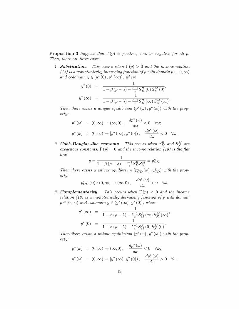
Proposition 3 Suppose that Γ (p) is positive, zero or negative for all p.Then, there are three cases.

1. Substitution. This occurs when Γ (p) > 0 and the income relation(18) is a monotonically increasing function of p with domain p ∈ [0,∞)and codomain y ∈ [y∗ (0) , y∗ (∞)), where

y∗ (0) =1

1− β (ρ− λ)− −1SRM (0)S

MX (0)

,

y∗ (∞) =1

1− β (ρ− λ)− −1SRM (∞)SM

X (∞).

Then there exists a unique equilibrium (p∗ (ω) , y∗ (ω)) with the prop-erty:

p∗ (ω) : (0,∞)→ (∞, 0) ,dp∗ (ω)

dω< 0 ∀ω;

y∗ (ω) : (0,∞)→ [y∗ (∞) , y∗ (0)) , dy∗ (ω)

dω< 0 ∀ω.

2. Cobb-Douglas-like economy. This occurs when SRM and SM

X areexogenous constants, Γ (p) = 0 and the income relation (18) is the flatline

y =1

1− β (ρ− λ)− −1SRMSMX

≡ y∗CD.

Then there exists a unique equilibrium (p∗CD (ω) , y∗CD) with the prop-

erty:

p∗CD (ω) : (0,∞)→ (∞, 0) ,dp∗ (ω)

dω< 0 ∀ω.

3. Complementarity. This occurs when Γ (p) < 0 and the incomerelation (18) is a monotonically decreasing function of p with domainp ∈ [0,∞) and codomain y ∈ (y∗ (∞) , y∗ (0)], where

y∗ (∞) =1

1− β (ρ− λ)− −1SRM (∞)SMX (∞)

,

y∗ (0) =1

1− β (ρ− λ)− −1SRM (0)S

MX (0)

.

Then there exists a unique equilibrium (p∗ (ω) , y∗ (ω)) with the prop-erty:

p∗ (ω) : (0,∞)→ (∞, 0) ,dp∗ (ω)

dω< 0 ∀ω;

y∗ (ω) : (0,∞)→ [y∗ (∞) , y∗ (0)) , dy∗ (ω)

dω> 0 ∀ω.

19

Proof. See the Appendix.

I refer to the second case as the Cobb-Douglas-like economy becausethis seemingly special configuration, requiring R

M = 1 +¡1− M

X

¢SRM , is in

fact quite common in the literature as it occurs when both technologies areCobb-Douglas and M

X = RM = 1.

Notice how the effect of resource abundance on the resource price is neg-ative in all cases while the effect on expenditure changes sign according tothe substitution possibilities between labor and materials in manufacturingand between labor and the natural resource in materials production. Thisbrings us to the observation that if Γ (p) changes sign for some p, the modelgenerates endogenously a switch from, say, complementarity to substitu-tion. I illustrate this case in Figure 2 where the income relation (18) is ahump-shaped function of p. The pattern is best captured by looking at theproperties of the function Γ (p). Using the definitions in Lemma 2, we have

dΓ (p)

dp= −d

MX (PM)

dPM

dPMdp

SRM (p)

+¡1− M

X (PM)¢ ¡1− R

M (p)¢− d R

M (p)

dp.

This derivative is negative if the following two conditions hold:

• the elasticities MX and R

M are increasing in PM and p, respectively;

• the terms 1− MX and 1− R

M have opposite sign.

The hump-shaped income relation in Figure 2 then obtains if Γ (0) > 0 andΓ (∞) < 0. Notice that the second condition says that if demand in onesector is elastic, say 1 < M

X , then demand in the other sector is inelastic,1 > R

M . Below I show that these conditions hold quite naturally in aneconomy with CES technologies. Here I discuss the general property.

Proposition 4 Suppose that there exists a price p where Γ (p) changes sign,from positive to negative, so that the income relation (18) is a hump-shapedfunction of p with domain p ∈ [0,∞) and codomain y ∈ [y∗ (0) , y∗ (∞)) ory ∈ [y∗ (∞) , y∗ (0)), where

y∗ (0) =1

1− β (ρ− λ)− −1SRM (0)S

MX (0)

,

y∗ (∞) =1

1− β (ρ− λ)− −1SRM (∞)SM

X (∞).

20

Then there exists a unique equilibrium (p∗ (ω) , y∗ (ω)) with the property:

p∗ (ω) : (0,∞)→ (∞, 0) ,dp∗ (ω)

dω< 0 ∀ω;

y∗ (ω) : (0,∞)→ [y∗ (∞) , y∗ (0)) , dy∗ (ω)

dωR 0 ω Q ω,

where ω is the value of ω such that p∗ (ω) = p.

Proof. See the Appendix.

The main message of this analysis is that resource abundance raises ex-penditure, and thereby results into a larger market for manufacturing goods,when the economy exhibits overall substitution between labor and resources(processed and raw) in the manufacturing of consumption goods and theprocessing of the natural resource into materials. Conversely, when theeconomy exhibits overall complementarity resource abundance results intoa smaller market for manufacturing goods. More importantly, whether theeconomy exhibits substitution or complementarity depends on equilibriumprices and thus on the endowment ratio itself. In other words, there aresolid reasons to expect that the effect of the endowment ratio on the pathof consumption is non-monotonic.

5.2 The path of consumption and welfare

For concreteness, consider an economy in steady state (p∗, y∗) and imaginean increment dω in its endowment ratio. Then, by construction we have

∆∗ =y∗ (ω) + dy∗(ω)

dω

y∗ (ω)− 1 = 1

y∗ (ω)

dy∗ (ω)

dω

and we can use the results of the previous section in a straightforward man-ner. Let us look first at the initial effect on consumption.

Proposition 5 The impact effect of the change in the endowment ratio is

d log³y∗(ω)c∗(ω)

´dω

= [Γ (p∗ (ω))−Ψ (p∗ (ω))]ωdp∗ (ω)

dω, (30)

where

Ψ (p∗ (ω)) ≡( − 1) y∗ (ω) = κ− SR

M (p∗ (ω))SMX (p∗ (ω)) ,

κ ≡ − 1 [1− β (ρ− λ)] .

21

Proof. See the Appendix.

Equation (27), Proposition 5 and the fact that dp∗(ω)dω < 0 ∀ω then yield

three possible configurations for the path of consumption:

1. Γ (p∗ (ω)) < 0 < Ψ (p∗ (ω)). The initial jump is up and then we havea growth acceleration. There is no “curse” and welfare rises.

2. 0 < Γ (p∗ (ω)) < Ψ (p∗ (ω)). The initial jump is up and then we havea growth deceleration. The welfare change is ambiguous since we havean intertemporal trade-off. Is the “curse” a curse?

3. 0 < Ψ (p∗ (ω)) < Γ (p∗ (ω)). The initial jump is down and then wehave a growth deceleration. Welfare falls. The “curse” is a curse.

Figure 3 illustrates these possibilities. Case 2 highlights the need to look atwelfare directly to resolve the ambiguity.

Proposition 6 The welfare effect of a change in the endowment ratio is

dU∗ (ω)

dω=

1

ρ− λ[(1 + μ)Γ (p∗ (ω))−Ψ (p∗ (ω))]ωdp

∗ (ω)

dω. (31)

Proof. See the Appendix.

We can then characterize four scenarios for welfare.

1. There is no curse — with or without quotation marks. This happenswhen

(1 + μ)Γ (p∗ (ω)) < Γ (p∗ (ω)) ≤ 0 < Ψ (p∗ (ω))and the rise of the endowment ratio generates a growth accelerationassociated to an initial jump up in consumption.14

2. There is a “curse”, in that the rise of the endowment ratio causesa growth deceleration, but the deceleration is offset by the fact thatresource abundance reduces prices and raises the level of consumption.This happens when

0 < Γ (p∗ (ω)) < (1 + μ)Γ (p∗ (ω)) < Ψ (p∗ (ω)) .

In this case the “curse” is not a curse.14Notice that this includes the Cobb-Douglas economy since in that case 1 = M

X = RM

and growth does not respond to ω at all while lower prices yield higher utility.

22

3. The “curse” is a curse. This happens when

0 < Γ (p∗ (ω)) < Ψ (p∗ (ω)) < (1 + μ)Γ (p∗ (ω))

and the rise of the endowment ratio generates a growth decelerationthat dominates over the initial jump up in consumption.

4. The “curse” truly is a curse. This worst-case scenario happens when

0 < Ψ (p∗ (ω)) < Γ (p∗ (ω)) < (1 + μ)Γ (p∗ (ω))

and the rise of the endowment ratio generates a growth decelerationassociated to an initial fall of consumption.

One of course is interested in mapping these scenarios into values of theendowment ratio itself. To do this, it is useful to impose some more structureon the model.

5.3 A CES economy

Consider the following CES economy:

Xi = Zθi [ψX (LXi − φ)σX + (1− ψX)M

σXi ]

1σX , σX ≤ 1;

M =£ψMLσM

M + (1− ψM)RσM¤ 1σM , σM ≤ 1.

The associated unit-cost functions are:

CXi = Z−θi

∙ψ− 1σX−1

X WσX

σX−1 + (1− ψX)− 1σX−1 P

σXσX−1M

¸σX−1σX

;

CM =

∙ψ− 1σM−1

M WσM

σM−1 + (1− ψM)− 1σM−1 p

σMσM−1

¸σM−1σM

;

From these one derives (recall that W ≡ 1):

SMX =

1

1 +³

ψX1−ψX

´ 11−σX P

σX1−σXM

; MX = 1 +

σX1− σX

¡1− SM

X

¢;

SRM =

1

1 +³

ψM1−ψM

´ 11−σM p

σM1−σM

; RM = 1 +

σM1− σM

¡1− SR

M

¢.

23

As is well known, the CES contains as special cases the linear productionfunction (σ = 1) wherein inputs are perfect substitutes, the Cobb-Douglas(σ = 0) wherein the elasticity of substitution between inputs is equal to 1,and the Leontief (σ = −∞) wherein inputs are perfect complements. Theadvantage of the CES specification, then, is that we can make things quiteexplicit and at the same time general.

Specifically, define:

Γ (ω) ≡ Γ (p∗ (ω)) =¡1− M

X (p∗ (ω))

¢SRM (p

∗ (ω)) + 1− RM (p

∗ (ω)) ;

Ψ (ω) ≡ Ψ (p∗ (ω)) = κ− SRM (p

∗ (ω))SMX (p∗ (ω)) .

Observe that if σX > 0 and σM > 0, then Γ (p) < 0 for all p and the “curse”never occurs. If σX < 0 and σM < 0, instead, Γ (p) > 0 for all p and the“curse” always occurs. Interestingly, if σX and σM have opposite signs wecan capture how the economy moves from one case to the other as the en-dowment ratio changes. Specifically, let σX > 0 and σM < 0 so that themanufacturing sector exhibits gross substitution between labor and materi-als while the resource sector exhibits gross complementarity between laborand raw resources. Recall that this means that demand for processed re-sources, i.e., materials, in the manufacturing sector is elastic, while demandfor raw resources in the primary sector is inelastic. We then have:

1. There is no “curse” and hence no curse. This happens when

Γ (ω) ≤ 0⇔ 0 < ω < ω.

2. The “curse” is not a curse. This happens when

0 < (1 + μ)Γ (ω) < Ψ (ω)⇔ ω < ω < ω.

3. The “curse” is a curse. This happens when

0 < Ψ (ω) < (1 + μ)Γ (ω)⇔ ω < ω <∞.

Figure 4 illustrates this analysis. The appendix establishes formally theproperties of the curves Γ (ω) and Ψ (ω) used in the figure to find the thresh-old values of the endowment ratio. Here I focus on the economics.

First, and most important: Why does the overall pattern of substitu-tion/complementarity matter so much for growth and welfare? Because itregulates the reduction in the price p required for the economy to absorb

24

the extra endowment of R relative to L. Notice, moreover, that the primaryand manufacturing sectors are vertically related so the adjustment involvesthe interdependent responses of PM to the increase in supply of processedresources and of p to the increase in supply of raw resources. Now, inelasticdemand means that the price has to fall drastically to induce the market toabsorb the additional quantity. Hence, if demand is inelastic in both sectorsthe overall adjustment requires drastic drops in both PM and p. What mat-ters is that the drastic fall of p results in a fall of resources income pω whichdepresses expenditure y. This is the case Γ > 0. In contrast, if demand iselastic in both sectors the overall adjustment requires mild drops in prices.The crucial difference is that in this case Γ < 0 so that resources income pωrises because the quantity effect dominates the price effect.

With this intuition in hand, we can now interpret the analytical results ofthe model. The function Γ (ω) starts out negative and increases monoton-ically, changing sign at ω and converging to its positive upper bound asω →∞. To see this, write

Γ0 (ω) =dΓ (p∗)

dp∗dp∗

dω

and observe that the CES economy with σX > 0 and σM < 0 satisfiesthe conditions for dΓ (p) /dp < 0 ∀p discussed above, namely: M

X > 1 andincreasing in PM ; R

M < 1 and increasing in p.The function Ψ (ω) is hump-shaped with a peak exactly at ω, where Γ (ω)

changes sign. The reason is that this is the value where the derivative ofSRM (p)S

MX (p) with respect to p equals zero. Notice also that Γ (ω) < Ψ (ω)

for all ω (see the appendix for the proof) so that Case 3 from figure 3and Scenario 4 from the analysis of welfare no longer apply because initialconsumption cannot fall.

The resulting pattern is the following: The endowment ratio is initiallyvery low and prices are very high, that is, ω → 0 ⇒ p → ∞ ⇒ PM =CM (1, p) → ∞. Under these conditions, Γ (0) < 0 < Ψ (0) so that anincrease in ω produces a growth acceleration associated to a jump up ininitial consumption. Intuitively, this says that in a situation of extremescarcity and extremely high price a helicopter drop of natural resource isgood. As the relative endowment grows, the overall pattern of substitutionchanges. In particular, Γ (ω) changes sign at ω = ω and we enter the regionwhere we get a “curse of natural resources” because an increase in resourceabundance yields a decrease in expenditure on manufacturing goods thattriggers a slowdown of TFP growth. This, “curse”, however, is not reallya curse since we are to the left of ω and the slowdown is associated to an

25

initial jump up in consumption that dominates in the intertemporal trade-off. As we keep moving to the right and enter the next region, ω < ω <∞, the growth deceleration is again associated to an initial jump up inconsumption but now the deceleration dominates in the intertemporal trade-off and welfare falls. It is here that we have a curse.

An effective summary of this pattern is to picture growth and welfareas hump-shaped functions of resource abundance. To do this, we first musttranslate the path of the log of TFP into a measure of average growth inline with what is considered in the empirical literature. Specifically, let

g (0, t) ≡ 1t[log T (t)− logT0]

be the average growth rate of TFP between time 0 and time t. Then, using(26) we have:

g (0, t) = g∗ +

µγ

ν+

1

− 1

¶∆∗1− e−νt

t. (32)

This says that the an increase in the endowment ratio is associated to atransitory period of above (below) trend average growth if it generates anincrease (decrease) in per capita expenditure on consumption goods. Noticethat as t → ∞ this measure converges to g∗, which does not depend on ωbecause there is no scale effect. Notice also, that since it depends on ω onlythrough ∆∗ it is hump-shaped in ω with the maximum at ω = ω.

For welfare we have two options. We can use the measure U∗ calculatedin (28), which is clearly hump-shaped in ω with the maximum at ω = ω. Wethen conclude directly that the peak of growth occurs earlier than the peakof welfare. This property captures the crucial role of initial consumption,which rises with resource abundance, in disposing of the growth = welfaretacit assumption. As equation (28) makes clear, welfare depends on thewhole path of consumption, not on a summary statistic of its slope.

One could argue that using (32) and (28) is inappropriate as they aresummary statistics computed over different time intervals. The alternativeis to compute welfare as the discounted integral of the same part of theconsumption path that we use to compute (32), that is,

U∗ (0, t) =

Z t

0e−(ρ−λ)s log u∗ (s) ds.

Using (26), (27) and (32), we can write

U∗ (0, t) = (a1 − a3) g∗ + a2 · log

µy∗

c∗

¶+ a3 · g (0, t) ,

26

where

a1 ≡Z t

0e−(ρ−λ)ssds; a2 ≡

Z t

0e−(ρ−λ)sds; a3 ≡

tR t0 e−(ρ−λ)s (1− e−νs) ds

1− e−νt.

This more algebra-intensive exercise does not change the conclusion: thetwo summary statistics differ because the former excludes the initial jumpin consumption. It is then obvious that at ω = ω the derivative of U∗ (0, t)with respect to ω is still positive and welfare is still rising. An intriguingproperty of the expression above is that it includes only items that in prin-ciple are observable so that one can do quick, back-of-the-envelope welfarecalcuations.

5.4 The reallocation

One is interested in knowing how the outcomes above relate to the economy’sreallocation of labor across sectors. Using (16) we have

LM

L= y

− 1SMX

¡1− SR

M

¢.

It is then easy to show that (see the Appendix)

d

dω

µLM

L

¶> 0 ∀ω,

so that, intuitively, resource abundance yields a reallocation of labor frommanufacturing to primary production. This result implies that

LX

L+

LZ + LN

L= 1− LM

L

falls to its new steady state value when ω increases.This is an interesting property as it says that there is a reallocation of la-

bor from production of manufacturing goods to production of materials, butthat this reallocation is not necessarily associated to a TFP slowdown. Thisis a fundamental difference between this model and models that generatethe curse of natural resources by tying productivity growth to manufactur-ing employment through learning by doing mechanisms.

Since the inter-sectoral reallocation is instantaneous, the dynamics thatdrive the time path of TFP take place within manufacturing. Equations(4), (14) and the formulation of the entry cost yield that the R&D share of

27

employment is

LZ + LN

L=

LZ

L+

N

L· β Y

N

=

∙1 − β (ρ− λ+ δ)

¸y − φn.

Recall that y jumps on impact to its new steady state value y∗ while n ispredetermined and does not jump. Then, using (24) at any time t we have

LZ + LN

L=

∙1 − β (ρ− λ+ δ)

¸y∗ − φn∗

1 + e−νt∆∗.

The new steady state value isµLZ + LN

L

¶∗= y∗

∙∙1 − β (ρ− λ+ δ)

¸− φ

n∗

y∗

¸,

where we know from the analysis of section 3 that n∗

y∗ is independent of ω.Thus, when the economy experiences a growth acceleration (deceleration)because y∗ rises (falls), the R&D share of employment jumps up (down)and converges from above (below) to a permanently higher (lower) value.Obviously, then, the ratio LX

L jumps down (up) and converges from below(above) to a permanently lower (higher) value.

5.5 Other interesting considerations

It is also interesting to study in some detail the role of measures of abun-dance and specialization. I consider the following two measures of resourceabundance that are close analogs to measures that have been studied in theempirical literature: the value of natural wealth as a share of GDP andthe value of natural wealth per capita. Notice that since A = βY and y isconstant, in this economy (nominal) GDP is

GDP = Y + A = Y + βY = Y (1 + βλ) .

Then, my two measures of abundance are:

pΩ

L= pω;

pΩ

GDP=

pω

(1 + βλ) y.

28

Differentiation yields:

d (pω)

dω= (ω + 1) pωΓ

dp

dω;

d

dω

µpΩ

GDP

¶=

1

(1 + βλ) y

∙d (pω)

dω− pω

y

dy

dω

¸=

pω

(1 + βλ) yΓdp

dω.

Notice how for both measures the effect of a change in ω necessarily has thesame sign as the effect on expenditure,

∆∗ =1

y∗ (ω)

dy∗ (ω)

dω= ωΓ

dp

dω.

The model, in other words, predicts a positive correlation between naturalwealth (per unit of GDP or per capita) and growth whether the “curse”occurs or not. It thus suggests that the positive correlation reported in thepapers mentioned in the introduction does not provide sufficient informa-tion to assess the underlying economic mechanism – which here is drivenby an income effect in which the adjustment of the resource price plays acrucial role – without specifying further what restrictions one imposes onthe endogenous variables that show up in these measures.

For example, Brunneschewiler and Bulte (2007) note that there is acrucial difference between the two measures of abundance in that the latterhas an endogenous variable at the denominator while the former does not.They argue that institutional factors drive down both the level and thegrowth rate of GDP per capita, so that it is quite possible that the ratiopΩ

GDP rises and regressions that do not control for its endogeneity reveal anegative correlation between growth and this measure of abundance. Theythus suggest that one should use the former measure because it is not subjectto this problem, and they show that doing so produces a positive correlationwith growth. From this result they infer that the “curse” does not exist.The premise of this line of reasoning – that the endogeneity of the level ofGDP at the denominator of the second measure of abundance must be takeninto account – is absolutely correct. My analysis, however, shows that thefirst measure is not immune from endogeneity issues either, since it containsthe price of the natural resource. Thus, the inference that the “curse” doesnot exist is correct if we know that the price effect is zero so that an increasein ω surely yields higher resource income. To my knowledge, the question ofwhether the data on natural capital used in this type of regressions supportssuch an assumption has not been investigated.15

15This strikes me as a first-order question since much of the debate hinges on the per-

29

It is also interesting to study the value of primary production as a shareof GDP since it is a relatively close analog of the export-based measures ofspecialization considered in the literature. Using (12) and (15), I have

PMM

GDP=

−1

1 + βλSMX

so that

d

dω

µPMM

GDP

¶=

−1

1 + βλ

dSMX

dPM

dPMdp

dp

dω=

−1

1 + βλ

¡1− M

X

¢ dpdω

.

Thus, if 1 < MX this derivative is positive and the increase of the share is as-

sociated to either a growth acceleration or a growth deceleration dependingon what happens to y, i.e., on whether Γ < 0 or Γ > 0. Similarly, if 1 > M

X

this derivative is negative and the decrease of the share is associated to eithera growth acceleration or a growth deceleration depending on whether Γ > 0or Γ < 0. The model, in other words, says that the sign of the correlationbetween growth and the share of the primary sector in GDP depends onthe properties of the overall pattern of substitution in manufacturing andresources processing and one cannot interpret the results of regression ex-ercises without further information on the function Γ (p) and its individualcomponents, in particular, M

X (p). The important point, therefore, is thatthe correlation between growth and the share of primary production in GDPdoes not provide sufficient information to assess the underlying mechanism.

Notice, however, that Γ and its individual components are observableso that the model provides specific guidelines for the derivation of testablepredictions. The most obvious is that one should sort economies accordingto M

X and Γ as the sign of the regression coefficient depends on these val-ues. For example, if we stipulate (and document empirically) that demandfor processed resources is elastic in all economies in the sample, then thediscriminating factor is whether the elasticity of demand for raw resourcesin the primary sector, R

M , and the share of resources in primary producers’costs, SR

M , yield Γ > 0 or Γ < 0.

formance of oil, gas or mineral exporting countries. Is it a fact that the discovery of newreserves of some resource in some country does not affect the world price of the resource?Even under price-taking behavior by the country’s suppliers, the country’s overall effecton the world price can be non-negligible.

30

6 Conclusion

The debate on whether natural resource abundance is good or bad for thelong-run fortunes of the economy is almost as old as economics itself. Themodern incarnation, spurred by the work of Sachs and Warner (1995, 2001),hinges on the sign of the coefficient of measures of resource abundance ingrowth regressions. Differently from the past, thus, it is much more drivenby solid and systematic econometric work. This is the clearest benefit ofthe comprehensive data sets now available. As this evidence accumulatesand adds to the already existing large body of historical information andanalyses, a definitive answer might finally emerge. We are not there yet,and the debate rages on.

One striking feature of this debate – and of the associated theoreticalliterature – is that at its heart is a tacit assumption growth = welfarethat is rarely, if ever, taken to task. Yet, the notion that growth and welfareare different is the cornerstone of modern growth theory. Moreover, naturalresource abundance is positively related to initial income in the very datathat researchers use to debate whether it is positively or negatively relatedto subsequent growth. Accordingly, it is not obvious at all that the “curseof natural resources” is, in fact, a curse.

In this paper, I developed a model of endogenous growth that allowed meto focus on the role of the intertemporal trade-off in determining whether theeffects of natural resource abundance on initial income and growth yield anincrease or a decrease in welfare. It is only in the latter case that the “curse”is indeed a curse. I found that resource abundance has non-monotonic effectson growth and welfare. More precisely, growth and welfare are hump-shapedfunctions of resource abundance. The property that the peak of growthoccurs earlier than the peak of welfare captures the crucial role of initialconsumption, which rises with resource abundance, and is an importantreminder that the welfare effect of resource abundance depends on the wholepath of consumption, not on a summary statistic of its slope. This reminderapplies to all explanations of the “curse” – institution-based, reallocation-based or any other type that future researchers will develop.

If resource abundance means that we sacrifice growth to boost currentconsumption, it stands to reason that to figure out whether we are better orworse off requires us to resolve the intertemporal trade-off. Consequently,growth regressions that ignore the effect of resource abundance on initialincome provide only one piece of the puzzle, not the solution. This is not asimple restatement of the fact that correlation is not causation. We cannotinfer from the negative correlation between resource abundance and growth

31

that resource abundant economies are worse off even if we can establishbeyond reasonable doubt that the relation is indeed negative and causal.

7 Appendix

7.1 The typical firm’s behavior

To characterize the typical firm’s behavior, consider the Current ValueHamiltonian

CVHi = [Pi − CX(1, PM)Z−θi ]Xi − φ− LZi + ziαKLZi ,

where the costate variable, zi, is the value of the marginal unit of knowledge.The firm’s knowledge stock, Zi, is the state variable; R&D investment, LZi ,and the product’s price, Pi, are the control variables. Firms take the publicknowledge stock, K, as given.

Since the Hamiltonian is linear, one has three cases. The case 1 > ziαKimplies that the value of the marginal unit of knowledge is lower than itscost. The firm, then, does not invest. The case 1 < ziαK implies thatthe value of the marginal unit of knowledge is higher than its cost. Sincethe firm demands an infinite amount of labor to employ in R&D, this caseviolates the general equilibrium conditions and is ruled out. The first orderconditions for the interior solution are given by equality between marginalrevenue and marginal cost of knowledge, 1 = ziαK, the constraint on thestate variable, (8), the terminal condition,

lims→∞

e−R st [r(v)+δ]dvzi(s)Zi(s) = 0,

and a differential equation in the costate variable,

r + δ =zizi+ θCX(1, PM)Z

−θ−1i

Xi

zi,

that defines the rate of return to R&D as the ratio between revenues fromthe knowledge stock and its shadow price plus (minus) the appreciation(depreciation) in the value of knowledge. The revenue from the marginalunit of knowledge is given by the cost reduction it yields times the scale ofproduction to which it applies. The price strategy is

Pi = CX(1, PM)Z−θi − 1 . (33)

32

Peretto (1998, Proposition 1) shows that under the restriction 1 > θ ( − 1)the firm is always at the interior solution, where 1 = ziαK holds, andequilibrium is symmetric.

The cost function (7) gives rise to the conditional factor demands:

LXi =∂CX(W,PM)

∂WZ−θi Xi + φ;

Mi =∂CX(W,PM)

∂PMZ−θi Xi.

Then, the price strategy (33), symmetry and aggregation across firms yield(11) and (12).

Also, in symmetric equilibrium K = Z = Zi yields K/K = αLZ/N ,where LZ is aggregate R&D. Taking logs and time derivatives of 1 = ziαKand using the demand curve (5), the R&D technology (8) and the pricestrategy (33), one reduces the first-order conditions to (13).

Taking logs and time-derivatives of Vi yields

r + δ =ΠXi

Vi+

ViVi,

which is a perfect-foresight, no-arbitrage condition for the equilibrium of thecapital market. It requires that the rate of return to firm ownership equalthe rate of return to a loan of size Vi. The rate of return to firm ownership isthe ratio between profits and the firm’s stock market value plus the capitalgain (loss) from the stock appreciation (depreciation).

In symmetric equilibrium the demand curve (5) yields that the cost ofentry is β Y

N . The corresponding dmand for labor in entry is LN = Nβ YN .

The case V > β YN yields an unbounded demand for labor in entry, LN =

+∞, and is ruled out since it violates the general equilibrium conditions.The case V < β Y

N yields LN = −∞, which means that the non-negativityconstraint on LN binds and N = 0. Free-entry requires V = β Y

N . Using theprice strategy (33), the rate of return to entry becomes (14).

7.2 The economy’s resources constraint

I now show that the household’s budget constraint reduces to the economy’slabor market clearing condition. Starting from (2), recall that A = NV and(r + δ)V = ΠX + V . Substituting into (2) yields

NV = NΠX + L+ pΩ+ΠM − Y.

33

Observing that NΠX = NPX − LX − LZ − PMM , NPX = Y , ΠM =PMM−LM −pR, R = Ω, and that the free entry condition yields that totalemployment in entrepreneurial activity is LN = NV , this becomes

L = LN + LX + LZ + LM .

7.3 Proof of Proposition 1

Taking logs of (25) yields

logT (t) = θ logZ0 + θ

Z t

0Z (s) ds+

1

− 1 logN (t) .

Using the definition n ≡ Ne−λt and adding and subtracting Z∗ from Z (t)yields

logT (t) = θ logZ0 + gt+ θ

Z t

0

hZ (s)− Z∗

ids+

1

− 1 logn (t) .

Using (19) the integral becomes

θ

Z t

0

³Z (s)− Z∗

´ds = θ

αθ ( − 1) Z t

0

µy∗

n (s)− y∗

n∗

¶ds

= γ

Z t

0

µn∗

n (s)− 1¶ds,

where

γ ≡ θαθ ( − 1) y∗

n∗= θ

αθ ( − 1) φ− ρ+δα

1−θ( −1) − ρβ.

Finally, (24) and the definition of ∆∗ yield

θ

Z t

0

³Z (s)− Z∗

´ds = γ

Z t

0e−νs

µn∗

n0− 1¶ds

=γ

ν∆∗¡1− e−νt

¢.

Using this result and (24) again, and noting that by construction T0 =

Zθ0n

1−10 since n0 = N0e

−λ·0 = N0, yields

log T (t) = logT0 + g∗t+γ∆∗

ν

¡1− e−νt

¢+

1

− 1 log1 +∆∗

1 + e−νt∆∗.

34

Next consider

log u∗ (t) = log− 1

+ log

µy∗

c∗

¶+ logT (t)

and use the expression just derived to write

log u∗ (t) = logy∗

c∗+ g∗t+

γ∆∗

ν

¡1− e−νt

¢+

1

− 1 log1 +∆∗

1 + e−νt∆∗.

Substituting this expression into (1) yields

U∗ =

Z ∞

0e−(ρ−λ)t log u∗ (t) dt

=

Z ∞

0e−(ρ−λ)t

∙log

µy∗

c∗

¶+ g∗t

¸dt

+γ

ν∆∗Z ∞

0e−(ρ−λ)t

¡1− e−νt

¢dt

+1

− 1

Z ∞

0e−(ρ−λ)t log

1 +∆∗

1 + e−νt∆∗dt.

The first and second integrals have straightforward closed form solutions; thethird has a complicated solution involving the hypergeometric function. Formy purposes, it is useful to introduce the following approximation that allowsme to simplify the expression for welfare. Since in general log (1 + x) ' x, Ican rewrite

log1 +∆∗

1 + e−νt∆∗= log (1 +∆∗)− log

¡1 + e−νt∆∗

¢= ∆∗

¡1− e−νt

¢,

which yields (26), (27) and

U∗ =

Z ∞

0e−(ρ−λ)t

∙log

µy∗

c∗

¶+ g∗t

¸dt

+

µγ

ν+

1

− 1

¶∆∗Z ∞

0e−(ρ−λ)t

¡1− e−νt

¢dt,

which upon integration yields (28).

35

7.4 Proof of Lemma 2

Differentiating and manipulating terms yields:

∂¡SMX SR

M

¢∂p

=∂SM

X

∂pSRM +

∂SRM

∂pSMX

=∂SM

X

∂PM

PMSMX

· ∂PM∂p

p

PM· S

MX SR

M

p+

∂SRM

∂p

p

SRM

· SRMSM

X

p

=

∙∂SM

X

∂PM

PMSMX

· ∂PM∂p

p

PM+

∂SRM

∂p

p

SRM

¸SRMSM

X

p

=

∙∂SM

X

∂PM

PMSMX

· ∂CM

∂p

p

CM+

∂SRM

∂p

p

SRM

¸SRMSM

X

p.

Recalling that∂SM

X

∂PM

PMSMX

= 1− MX ,

∂SRM

∂p

p

SRM

= 1− RM ,

∂CM

∂p

p

CM= SR

M

and substituting into the expression above yields (29).

7.5 Proof of Proposition 3

Refer to Figure 1. In the case of complementarity, depicted in the upperpanel, we have the following pattern. For ω → 0 the expenditure line (17) isalmost, but not quite, flat and intersects the income relation (18) for p→∞and y → y∗ (∞). As ω grows, the expenditure line rotates counterclockwiseand the intersection shifts left, tracing the income relation. We thus obtainthat both p∗ and y∗ fall. As ω →∞, the expenditure line becomes verticaland the intersection occurs at p→ 0 and y → y∗ (0).

In the case of substitution in the lower panel, we have a similar patternwith the difference that the income relation now has negative slope so that asthe expenditure line rotates counterclockwise y∗ increases. Specifically, forω → 0 the expenditure line is almost, but not quite, flat and intersects theincome relation for p → ∞ and y → y∗ (∞). As ω grows, the expenditureline rotates counterclockwise and the intersection shifts left yielding that

36

p∗ falls while y∗ rises. As ω →∞, the expenditure line becomes vertical andthe intersection occurs at p→ 0 and y → y∗ (0).16

7.6 Proof of Proposition 4

Refer to Figure 2. The proof is essentially the same as above. The onlydifference is that as the expenditure line rotates it traces the hump-shapedincome relation yielding that p∗ always falls while y∗ rises for 0 < ω < ωand falls for ω < ω <∞.

7.7 Proof of Proposition 5

Observe first thatd log

¡yc

¢dω

=d log y

dω− d log c

dω.

Now,d log y

dω=

d log y

dp

dp

dω= ωΓ (p)

dp

dω

and

d log c

dω=

1

CX

dCX

dω=

1

CX

dCX

dPM

dPMdp

dp

dω

=PMCX

dCX

dPM

dPMdp

p

PM

1

p

dp

dω

=SMX SR

M

p

dp

dω.

16An interesting question is whether the model admits an equilibrium for ω = 0. Toinvestigate whether it does, it is useful to focus on the CES case considered in the text. Theanswer depends on wheteher resources are essential. Under σM < 0, σX < 0 they are andthus an equlibrium with ω = 0 (due to Ω = 0) cannot exist. To see this, notice that in thiscase SMX (0)SRM (0) = 0 and SMX (∞)SRM (∞) = 1 so that the representation in the upperpanel of Figure 1 applies with the difference that the expenditure and income relationshave the intercept y∗ (0) in common. (This point, obviously, is not an equilibrium.) Wethen have that for ω = 0 the expenditure line is exactly flat and there is no intersectionwith the income relation. If instead we posit σM > 0, σX > 0 we have SMX (0)SRM (0) > 0and SMX (∞)SRM (∞) = 0 and the representation in the lower panel of Figure 1 applies withthe crucial difference that the expenditure line starts out at y∗ (∞). Hence, for ω = 0 theline is exactly tangent to the horizontal asymptote of the income relation implying thatp =∞ and y∗ (∞) is a feasible equilibrium. This is because we now allow for substitutionso that processed natural resources are not essential in manufacturing and the economycan exist with Ω = 0.

37

Hence,d log

¡yc

¢dω

=

µΓ− SM

X SRM

pω

¶ωdp

dω.

which using (12) becomes (30).

7.8 Proof of Proposition 6

Observe that by construction

d∆∗

dω=1

y∗dy∗

dω

Differentiation of (28) then yields

dU∗

dω=

1

ρ− λ

⎡⎣d log³y∗

c∗

´dω

+ μ1

y∗dy∗

dω

⎤⎦=

1

ρ− λ

∙(1 + μ)

d log y∗

dω− d log c∗

dω

¸.

Using the expressions calculated above and rearranging terms yields (31).

7.9 The CES economy with σX > 0 and σM < 0

The Γ (ω) curve. Dropping stars to simplify notation, the equation is:

Γ (ω) =

∙− σX1− σX

¡1− SM

X (p (ω))¢+

σM1− σM

¸SRM (p (ω))−

σM1− σM

Proposition 4 yields that p (0) =∞ and p (∞) = 0. Therefore, for ω → 0:

SRM (0) = lim

p→∞1

1 +³

ψM1−ψM

´ 11−σM p

σM1−σM

= 1.

Also,

PM (0) = limp→∞

∙ψ

11−σMM + (1− ψM)

11−σM p

σMσM−1

¸σM−1σM

=∞,

so thatSMX (0) = lim

PM→∞

1

1 +³

ψX1−ψX

´ 11−σX P

σX1−σXM

= 0.

38

Consequently,

Γ (0) =−σX1− σX

< 0.

In contrast, for ω →∞:

SRM (∞) = lim

p→01

1 +³

ψM1−ψM

´ 11−σM p

σM1−σM

= 0.

Also,

PM (∞) = limp→0

∙ψ

11−σMM + (1− ψM)

11−σM p

σMσM−1

¸σM−1σM

= ψ− 1σM

M ,

so thatSMX (∞) = 1

1 +³

ψX1−ψX

´ 11−σX ψ

− 1σM

σX1−σX

M

.

Consequently,

Γ (∞) = −σM1− σM

> 0.

The next step is to show that the curve is monotonically increasing:

Γ0 (ω) =σX

1− σX·| z

+

dSMX

dPM| z ·−

dPMdp| z ·+

dp

dω|z ·−

SRM

+

∙− σX1− σX

¡1− SM

X

¢+

σM1− σM

¸| z ·

−

dSRM

dp| z ·+

dp

dω|z−

> 0.

Finally, notice that by continuity there exists a value ω where Γ (ω) = 0.The Ψ (ω) curve. Again dropping stars, the equation is:

Ψ (ω) = κ− SRM (p (ω))S

MX (p (ω)) .

The limiting behavior at 0 and ∞ is straightforward. The previous calcula-tions yield:

Ψ (0) = κ− SRM (0)S

MX (0) = κ;

Ψ (∞) = κ− SRM (∞)SM

X (∞) = κ.

39

Next observe that

Ψ0 (ω) =d¡SRM (p (ω))S

MX (p (ω))

¢dp (ω)

dp (ω)

dω

= Γ (ω)SRM (p (ω))S

MX (p (ω))

p (ω)

dp (ω)

dω,

so that the curve is hump-shaped with its maximum exactly at the value ωwhere Γ (ω) changes sign.

The threshold values. Observe that κ > 1 > −σM1−σM . It is evident

from Figure 2 then that Γ (ω) < Ψ (ω) ∀ω. It follows that there is only onerelevant intersection, of Ψ (ω) with (1 + μ)Γ (ω), that yields the thresholdvalue ω such that ω < ω.

7.10 The reallocation

The expression for the share of employment in the primary sector and theexpressions derived in the proofs above yield

d

dω

µLM

L

¶=

− 1"dy

dωSMX

¡1− SR

M

¢+ y

dSMX

dω−

d¡SMX SR

M

¢dω

#

=− 1

∙Γ

ΨSMX

¡1− SR

M

¢+ 1− M

X − Γ¸ωdp

dω.

Recall that dpdω < 0. Then

d

dω

µLM

L

¶> 0 ∀ω

because the term in brackets is

Γ

Ψ

¡SMX − κ

¢+ 1− M

X < 0

since κ > 1 and 1 − MX < 0 under the assumption that manufacturing

exhibits substitution between labor and materials.

References

[1] Alexeev M. and Conrad R., 2007, The Elusive Curse of Oil, De-partment of Economics, Indiana University, manuscript (available athttp://mypage.iu.edu/~malexeev/alexeev_conrad_rev_5-07.pdf).

40

[2] Banks R.B., 1994, Growth and Diffusion Phenomena, Berlin Heidel-berg, Springer-Verlag.

[3] Boyce J.R. and Emery J.C.H, What Can Exhaustible Resource TheoryTell Us About Per Capita Income Growth and Levels in Resource Abun-dant Economies?, Department of Economics, University of Calgary,manuscript (available at http://econ.ucalgary.ca/profiles/john-boyce).

[4] Bravo-Ortega C. and de Gregorio J., 2007, The Relative Richness of thePoor? Natural Resources, Human Capital, and Economic Growth, inNatural Resources: Neither Curse Nor Destiny, edited by D. Ledermanand W.F. Maloney, Stanford University Press.

[5] Brunneschweiler C.N. and Bulte E.H., 2007, The Resource Curse Re-visited and Revised: A tale of Paradoxes and Red Herrings, Journal ofEnvironmental Economics and Management (forthcoming).

[6] Etro F., 2004, Innovation by Leaders, Economic Journal, 114, 281-303.

[7] Gylfason T., 2001a, Lessons from the Dutch Disease:Causes, Treatment, and Cures, manuscript (available athttp://www.hi.is/~gylfason/pdf/statoil22.pdf).

[8] Gylfason T., 2001b, Natural Resources, Education, and Economic De-velopment, European Economic Review, 45, 847-859.

[9] Lederman D. and Maloney W.F. (eds.), 2007a, Natural Resources: Nei-ther Curse Nor Destiny, Stanford University Press.

[10] Lederman D. and Maloney W.F., 2007b, Trade Structure and Growth,in Natural Resources: Neither Curse Nor Destiny, edited by D. Leder-man and W.F. Maloney, Stanford University Press.

[11] Papyrakis E. and Gerlagh R., 2003, Natural Resources: A Blessing or aCurse?, Fondazione Eni Enrico Mattei, Nota di Lavoro 8.2003 (availableat http://www.feem.it/web/activ/_wp.html).

[12] Papyrakis E. and Gerlagh R., 2007, Resource Abundance and EconomicGrowth in the United States, European Economic Review, 51, 1011-1039.

[13] Peretto, P.F., 1998,. Technological Change and Population Growth,Journal of Economic Growth, 3, 283-311.

41

[14] Peretto P.F. and Connolly M., 2007, The Manhattan Metaphor, Journalof Economic Growth, 12, 329-350.

[15] Peretto P.F. and Smulders S., 2002, Technological Distance, Growthand Scale Effects, Economic Journal, 112, 603-624.

[16] Rodriguez F. and Sachs J.D., 1999, Why Do Resource-AbundantEconomies Grow More Slowly?, Journal of Economic Growth, 4, 277-303.

[17] Sachs J.D. and Warner A.M., 1995, Natural Resource Abundance andEconomic Growth, NBER WP 5398.

[18] Sachs J.D. and Warner A.M., 2001, The Curse of Natural Resources,European Economic Review, 45, 827-838.

[19] Sala-i-Martin X., 1997, I Just Run 2 Million Regressions, AmericanEconomic Review Papers and Proceedings, 87, 178-83

[20] Sala-i-Martin X., Doppelhofer G. and Miller R.I., 2004, Determinantsof Long-Run Growth: A Bayesian Averaging of Classical Estimates(BACE) Approach, American Economic Review, 94, 813-835.

[21] Smulders S., 2005, Endogenous Technological Change, Natural re-sources, and Growth, in Scarcity and Growth Revisited: Natural Re-sources and the Environment in the New Millennium, edited by H.Folmer and L. Gabel L., The Johns Hopkins University Press for Re-sources for the Future.

[22] Stevens P., 2003, Resource Impact — Curse or Blessing? A LiteratureSurvey, Journal of Energy Literature, IX, 3-42.

42

0=t

Case 1: Ψ<<Γ 0

Baseline path

Case2: Ψ<Γ<0

Case 3: Γ<Ψ<0

)(log * tu

t

Figure 3: The path of consumption

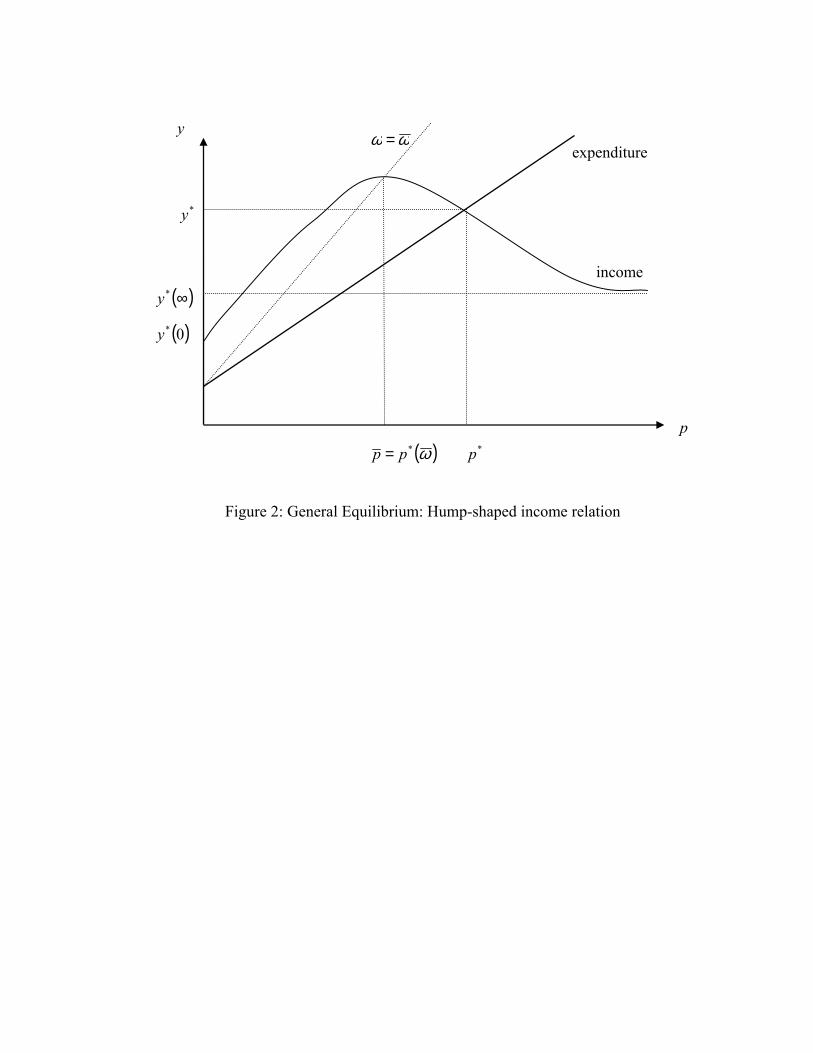
p

y

( )ω*pp =

expenditure

*y

( )∞*y

( )0*y

*p

ωω =

Figure 2: General Equilibrium: Hump-shaped income relation

income

p

y

p

*p

expenditure

expenditure

( )∞*y

*y

( )0*y

( )∞*y

( )0*y

*p

income *y

income

Figure 1: General Equilibrium: Monotonic income relation

ω ω~

( )ωΨ ( ) ( )ωµ Γ+1

κ

Figure 4: The endowment ratio and equilibrium outcomes

ω

X

X

σσ

−−

1

( )ωΓM

M

σσ

−−

1