Is Information Risk a Determinant of Asset Returns? · rational expectations equilibrium to...

Is Information Risk a Determinantof Asset Returns?

DAVID EASLEY, SOEREN HVIDKJAER, and MAUREEN O’HARA*

ABSTRACT

We investigate the role of information-based trading in affecting asset returns. Weshow in a rational expectation example how private information affects equilib-rium asset returns. Using a market microstructure model, we derive a measure ofthe probability of information-based trading, and we estimate this measure usingdata for individual NYSE-listed stocks for 1983 to 1998. We then incorporate ourestimates into a Fama and French ~1992! asset-pricing framework. Our main re-sult is that information does affect asset prices. A difference of 10 percentage pointsin the probability of information-based trading between two stocks leads to a dif-ference in their expected returns of 2.5 percent per year.

ASSET PRICING IS FUNDAMENTAL to our understanding of the wealth dynamics ofan economy. This central importance has resulted in an extensive literatureon asset pricing, much of it focusing on the economic factors that inf luenceasset prices. Despite the fact that virtually all assets trade in markets, oneset of factors not typically considered in asset-pricing models are the fea-tures of the markets in which the assets trade. Instead, the literature onasset pricing abstracts from the mechanics of asset price evolution, leavingunsettled the underlying question of how equilibrium prices are actuallyattained.

Market microstructure, conversely, focuses on how the mechanics of the trad-ing process affect the evolution of trading prices. A major focus of this exten-sive literature is on the process by which information is incorporated into prices.The microstructure literature provides structural models of how prices be-come efficient, as well as models of volatility, both issues clearly of importancefor asset pricing. But of perhaps more importance, microstructure models pro-

* Cornell University, University of Maryland, and Cornell University. The authors would liketo thank Anat Admati; Yakov Amihud; Kerry Back; Patrick Bolton; Douglas Diamond; KenFrench; William Gebhardt; Gordon Gemmill; Mark Grinblatt; Campbell Harvey; David Hirshle-ifer; Schmuel Kandell; Charles Lee; Bhaskaran Swaminathan; Zhenyu Wang; Ingrid Werner;two referees; the editor ~René Stulz!; and seminar participants at Cornell University, DePaulUniversity, the Federal Reserve Bank of Chicago, Georgia State University, the Hong KongUniversity of Science and Technology, INSEAD, the Massachusetts Institute of Technology,Princeton University, the Red Sea Finance Conference, the Stockholm School of Economics,Washington University, the University of Chicago, the University of Essex, the Western FinanceAssociation meetings, and the European Finance Association meetings for helpful comments.We are also grateful to Marc Lipson for providing us with data compaction programs.

THE JOURNAL OF FINANCE • VOL. LVII, NO. 5 • OCTOBER 2002

2185

vide explicit estimates of the extent of private information. The microstruc-ture literature has demonstrated the important link between this privateinformation and an asset ’s bid and ask trading prices, but it has yet to be dem-onstrated that such information actually affects asset-pricing fundamentals.

If a stock has a higher probability of private information-based trading,should that have an effect on its required return? In traditional asset-pricing models, the answer is no. These models rely on the notion that ifassets are priced “efficiently,” then information is already incorporated andhence need not be considered. But this view of efficiency is static, not dy-namic. If asset prices are continually revised to ref lect new information,then efficiency is a process, and how asset prices become efficient cannot beseparated from asset returns at any point in time.

That stock returns might depend upon features of the trading process hasbeen addressed in various ways in the literature. Perhaps the most straight-forward approach is that of Amihud and Mendelson ~1986!, who argue thatliquidity should be priced. Their argument is that investors maximize ex-pected returns net of transactions ~or liquidity! costs, where a simple mea-sure of these costs is the bid-ask spread. In equilibrium, traders will requirehigher returns to hold stocks with larger spreads. Amihud and Mendelson~1986, 1989! and Eleswarapu ~1997! present empirical evidence consistentwith this liquidity hypothesis. Supporting evidence using other measures ofliquidity is provided by Brennan and Subrahmanyam ~1996!, Amihud, Men-delson, and Lauterbach ~1997!, Brennan, Chordia, and Subrahmanyam ~1998!,Datar, Naik, and Radcliffe ~1998!, and Amihud ~2000!. But the overall re-search on this issue is mixed, with Eleswarapu and Reinganum ~1993!, Chenand Kan ~1996!, and Chalmers and Kadlec ~1998! concluding that liquidity isnot priced. Certainly, part of the difficulty in resolving this issue is simplythat transactions costs, however measured, are often quite small. While iden-tifying illiquidity with transactions costs seems sensible, finding these li-quidity effects among the noise in asset returns need not be an easy task.

Our focus in this paper is on showing empirically that a different aspect ofthe trading and price discovery process—private information—affects cross-sectional asset returns. We first present a simple example to provide theintuition for why the existence of private information should affect stockreturns.1 The importance of this information effect is then an empirical ques-tion. However, this question is difficult to answer because the extent of pri-vate information is not directly observable. To deal with this problem, weuse a structural market microstructure model to generate a measure of theprobability of information-based trading ~PIN! in individual stocks. We thenestimate this measure using high-frequency data for NYSE-listed stocks forthe period 1983 to 1998. The resulting estimates are a time series of indi-vidual stock probabilities of information-based trading for a very large cross

1 The theoretical case for why information affects asset returns is developed more fully inEasley and O’Hara ~2000!. We present in this paper a brief example of this cross-sectionaleffect.

2186 The Journal of Finance

section of stocks. We investigate whether these information probabilities af-fect cross-sectional asset returns by incorporating our estimates into a Famaand French ~1992! asset pricing framework.

Our main result is that information does affect asset prices: Stocks with higherprobabilities of information-based trading have higher rates of return. In-deed, we find that a difference of 10 percentage points in PIN between two stocksleads to a difference in their expected returns of 2.5 percent per year. The mag-nitude, and statistical significance, of this effect provides strong support forthe premise that information affects asset-pricing fundamentals.

Our focus on the role of information in asset pricing is related to severalrecent papers. In a companion theoretical paper, Easley and O’Hara ~2000!develop a multiasset rational expectations equilibrium model in which stockshave differing levels of public and private information. In equilibrium, un-informed traders require compensation to hold stocks with greater privateinformation, resulting in cross-sectional differences in returns. Admati ~1985!generalized Grossman and Stiglitz’s ~1980! analysis of partially revealingrational expectations equilibrium to multiple assets and showed how indi-viduals face differing risk-return trade-offs when differential information isnot fully revealed in equilibrium. Wang ~1993! provides an intertemporalasset-pricing model in which traders can invest in a riskless asset and arisky asset. In this model, the presence of traders with superior informationinduces an adverse selection problem, as uninformed traders demand a pre-mium for the risk of trading with informed traders. However, trading by theinformed investors also makes prices more informative, thereby reducinguncertainty. These two effects go in opposite directions, and their overalleffect on asset returns is ambiguous. Because this model allows only onerisky asset, it is not clear how, if at all, information would affect cross-sectional returns. Jones and Slezak ~1999! also develop a theoretical modelallowing for asymmetric information to affect asset returns. Their modelrelies on changes in the variance of news and liquidity shocks over time todifferentially affect agents’ portfolio holdings, thereby inf luencing asset re-turns. These theoretical papers suggest that asymmetric information canaffect asset returns, the issue of interest in this paper.

An alternative stream of the literature considers the effects of incomplete,but symmetric, information on asset prices. Building from Merton ~1987!, anumber of authors ~see, e.g., Basak and Cuoco ~1998! and Shapiro ~2002,p. 49!! analyze asset pricing when traders can be unaware of the existenceof some assets. In this setting, cross-sectional differences in returns can emergesimply because traders cannot hold assets they do not know about; the lackof demand for these unknown assets results in their commanding a higherreturn in equilibrium.2 The symmetric information structure here is an im-

2 A variant of this model is that traders face some exogenous participation constraints. Forexample, international investors may be unable to purchase assets that are available to domes-tic investors, and this can create cross-sectional differences in returns. A model that does allowasymmetric information in this setting is Brennan and Cao ~1997!.

Is Information Risk a Determinant of Asset Returns? 2187

portant difference between these models and our analysis. There is no riskof trading with traders who have better information because everyone knowsthe same information. Some traders may face participation constraints onholding some assets, but these constraints are not related to information onfuture asset performance. Indeed, as Merton pointed out, a problem with theincomplete information model is that any higher asset premium can be ar-bitraged away by traders who do not face such constraints. That is not thecase with our asymmetric information risk; the risk remains in equilibriumeven though all traders know it is there.

A related literature on estimation risk also examines the effect of differ-ential information on expected returns ~see Barry and Brown ~1984, 1985!,Barry and Jennings ~1992!, or Coles, Loewenstein, and Suay ~1995! for ex-amples!. This literature asks how differences in investor confidence aboutreturn distributions affects expected returns. The basic conclusion is thatsecurities for which there is little information will have higher expectedreturns. These securities are riskier for investors than securities about whichthey have more information, but this risk is different from that measured byb, and thus it affects measured excess returns. The difference between thisapproach and ours is that we focus on differences of information across in-vestors, each of whom knows the structure of returns, and we ask whetherhaving private versus public information affects security returns.

Finally, two recent empirical papers related to our analysis are Brennanand Subrahmanyam ~1996! and Amihud ~2000!. These authors investigatehow the slope of the relationship between trade volume and price changesaffects asset returns. This measure of illiquidity relies on the price impact oftrade, and it seems reasonable to believe that stocks with a large illiquiditymeasure are less attractive to investors. Brennan and Subrahmanyam findsupport for this notion using two years of transactions data to estimate theslope coefficient l, while Amihud establishes a similar finding using dailydata. What economic factors underlie this result is not clear. Because l isderived from price changes, factors such as the impact of price volatility ondaily returns, or inventory concerns by the market maker could inf luencethis variable, as could adverse selection.3 Neither analysis addresses whethertheir illiquidity measure is proxying for spreads, or for the more fundamen-tal information risk we address. Our analysis here focuses directly on pri-vate information by deriving a trade-based measure of information risk. This

3 The Kyle ~1985! l has not been tested as to its actual linkage with private information.While it seems reasonable to us that such a theoretical linkage would exist, there are a numberof reasons why this empirical measure is problematic. For example, the actual Kyle modelassumes a call market structure in which orders are aggregated and it is only the net imbal-ance that affects the price. Actual markets do not have this structure, so in practice l is esti-mated on a trade-by-trade basis ~as in Brennan and Subrahmanyam!, or is a time-series changein price per volume over some interval ~as in Amihud!. Either approach may introduce noise inthe specification. Moreover, because the l calculation also involves both price and the quantityof the trade, its actual value may be affected by factors such as the size of the book, tick sizeconsideration, and market maker inventory.


PIN measure has been shown in previous work ~see Easley, Kiefer, & O’Hara~1996a, 1997a, 1997b!!, Easley et al. ~1996b!, and Easley, O’Hara & Paper-man ~1998!! to explain a number of information-based regularities, provid-ing the link to private information we need to investigate cross-sectionalasset-pricing returns.

The PIN variable is correlated with other variables that we do not includein our return estimation. In particular, as would be expected with an infor-mation measure, PIN is correlated with spreads. It is also correlated withthe variability of returns and with volume or turnover. One might suspectthat the probability of information-based trade only seems to be priced be-cause it serves as a proxy for these omitted variables. We show, however,that this is not the case. We show that over our sample period, spreads donot affect asset returns but PIN does. When spreads or the variability ofreturns are included with PIN in the return regressions, the probability ofinformation-based trade remains highly significant, and its effect on returnsis changed only slightly. Volume remains a factor in asset pricing, but it doesnot remove the inf luence of PIN. We view these results as strong evidencethat the probability of information-based trade is priced in asset returns.

The paper is organized as follows. Section I provides the theoretical intu-ition for our analysis. We construct a partially revealing rational expectationexample in which private information affects asset prices because it skewsthe portfolio holdings of informed and uninformed traders in equilibrium.We then turn in Section II to the empirical testing methodology. We set outa basic microstructure model and we demonstrate how the probability ofinformation-based trading is derived for a particular stock. Estimation ofthe model involves maximum likelihood, and we show how to derive theseestimating equations. In Section III, we present our estimates. We examinethe cross-sectional distribution of our estimated parameters, and we exam-ine their temporal stability. Section IV then puts our estimates into an asset-pricing framework. We use the cross-sectional approach of Fama and French~1992! to investigate expected asset returns. In this section, we present ourresults, and we investigate their robustness. We also investigate the differ-ential ability of spreads, variability of returns, turnover, and our informa-tion measure to affect returns. Section V summarizes our results and discussestheir implications for asset-pricing research.

I. Information and Asset Prices

To show that whether information is private or public affects asset re-turns, we construct a simple rational expectations equilibrium asset-pricingexample. We use this example only to motivate our empirical search forinformation effects, so we keep the exposition here as simple as possible. Amore general analysis of the effects of public and private information onasset prices is found in a companion theoretical paper by Easley and O’Hara~2000!.


In standard capital-asset-pricing models ~CAPM!, individuals have com-mon beliefs, and assets are priced according to these beliefs. Market riskmust be held, and in equilibrium, individuals are compensated withgreater expected returns for holding it. But no one must hold idiosyncraticrisk, and so there is no market compensation for doing so. We show herethat when there is differential information that is not fully revealed inequilibrium, and individuals thus have differing beliefs, the story is morecomplex.

We begin with a simple example that we make more complex, and morerealistic, in three stages. First, we consider a market in which individualshave, for whatever reason, arbitrarily differing beliefs. These individualsperceive differing risk-return trade-offs in the market, and, most impor-tantly, they typically hold differing portfolios. Thus, they will rationally chooseto hold idiosyncratic risk. They believe that they are being compensated forholding this risk because they believe that assets are mispriced. Whetherthey are in fact compensated for holding idiosyncratic risk depends on howtheir beliefs relate to the truth. A trader with correct beliefs, in a world inwhich some others are incorrect, correctly perceives an expected excess re-turn to holding some assets and he overweights his portfolio, relative to themarket, in these assets.

We then drop the arbitrary beliefs assumption, and we generate differ-ences in beliefs from common priors and private information that is not fullyrevealed by equilibrium asset prices. In this second part of our example,there is nothing irrational about any of the individuals: They have commonpriors, they receive differing information, they make correct inferences fromtheir information and market prices, but they end up with differing beliefsas long as all information is not fully revealed. Individuals with privateinformation have better beliefs, that is, they correctly perceive expected ex-cess returns on some assets, and they hold better portfolios than do thosewithout private information. In this case, the existence of private informa-tion generates expected ~average! excess returns to some assets.

Third, we ask what happens if this private information is made public.Here the traders hold a common portfolio. They hold only market risk, notany idiosyncratic risk. We show that this reduces the expected excess re-turns to assets about which information was previously private. In this case,individuals are compensated only for holding market-wide risk whereas be-fore they were compensated for the extra risk induced by the private infor-mation. We conclude that private, rather than public, information can yieldan increase in required expected returns.

For our example, we consider a two-period, dates t and t 1 1, consumption-based asset-pricing model. There are two possible states of the world, s 51,2, at date t 1 1, and there are two assets with state contingent payoffs.Asset one pays three units of the single consumption good in state one andzero units in the other state; asset two pays three units of the good in statetwo and zero units in state one. Since each asset is identified with the statein which it pays off, we index both states and assets by s. Initially we con-


sider an economy in which there is one unit of each asset available. Theprice of the consumption good is one at each date and asset prices at date tare p 5 ~ p1, p2!.

There are two traders indexed by i 5 1,2. Each trader is endowed with oneunit of the consumption good and with one-half of the available assets. Trad-ers have logarithmic utility of consumption at dates t and t 1 1 and theydiscount future utility with discount factor 0 , r , 1. Trader i ’s belief aboutthe distribution of states tomorrow is qi 5 ~q1

i ,q2i !. Trader i chooses current

consumption and asset purchases, ~cti , a1

i , a2i !, to maximize his expected util-

ity of current and future state contingent consumption, ~cti , ct11

i ~1!, ct11i ~2!!,

ln~cti! 1 r@q1

i ln~ct11i ~1!! 1 q2

i ln~ct11i ~2!!# ~1!

subject to his budget constraints

cti 5 wt

i 2 p1 a1i 2 p2 a2

i , ct11i ~1! 5 3a1

i , ct11i ~2! 5 3a2

i , ~2!

where wti 5 1 1 ~ p1 1 p2!02 is date t wealth.

If the traders have common beliefs, q, then it is easy to show that equi-librium asset prices are ps

* 5 2qs r, and that, in equilibrium, each traderholds one-half a unit of each asset. Thus, the traders hold risk-free port-folios. There is no single risk-free asset in this economy, but traders cancreate one by buying equal amounts of the two risky assets. The shadowrisk-free rate ~of return! this implies is 302r21. So the price of asset s is itsexpected payoff, 3qs, divided by the risk-free rate, 302r21. As there is nomarket risk in the economy, this is just a simple example of the consumption-based CAPM.

If the traders have differing beliefs, similar calculations show that equi-librium prices are ps 5 2qsr where qs 5 102~qs

1 1 qs2! is the average belief

about the probability of state s. So again, the price of each asset is an ex-pected return divided by the risk-free rate ~the risk-free rate is still 302r21 !,but now the expectation is a market or average expectation—not any indi-vidual’s expectation. This is an example of Lintner ’s ~1969! generalization ofthe CAPM to heterogeneous beliefs. Although traders can still create a risk-free asset, they choose to hold idiosyncratic risk. This calculation shows thatequilibrium date t 1 1 consumptions for trader i in states one and two are~3q1

i 02q1,3q2i 02q2!. Unless beliefs are identical, traders have random date

t 1 1 consumptions even though there is no market risk in this economy.This occurs because each trader believes the assets are mispriced, and soeach trader is willing to accept some risk in order to take advantage of theperceived mispricing.

Suppose that trader one’s beliefs are, in fact, correct. Then the expectedreturn on asset s is 3qs

1. So asset prices are not ~correct! expected returnsdivided by the risk-free rate. There is a positive excess return ~expectedreturn divided by price minus the risk-free rate! on one asset and a negative


excess return on the other asset. This occurs even though there is no market-wide risk: There will be three units of the good tomorrow for sure. The traderwith better beliefs holds a better portfolio; he overweights his portfolio inthe asset with a positive excess return.

This simple example shows that if traders have differing beliefs they per-ceive differing risk-return trade-offs and they may choose to hold idiosyn-cratic risk. Each trader believes that he is being compensated for the risk heholds. In fact, at least one of these traders has incorrect beliefs. So his per-ceptions about the risk-return trade-off are also incorrect. Next, we intro-duce private information into the economy so that neither trader has incorrectbeliefs—they have a common prior and more or less information.4

The common prior on states is ~ 12_ , 1

2_ !. Trader one, the informed trader,

receives a private signal y [ $1,2% with probability 12_ on each signal. If y 5 1,

then the conditional probability of state one is 34_ , and if y 5 2, the conditional

probability of state one is 14_ . Trader two is uninformed, but he knows this

structure and he uses this knowledge, along with equilibrium prices, to makeany inferences that he can about the informed trader ’s information. Unlesswe introduce further randomness into the economy, prices will reveal theinformed trader ’s signal and, in equilibrium, traders will have common be-liefs. To prevent this uninteresting case, we use the standard device of noisysupply.5 The aggregate supply of assets one and two is given by the randomvariable x [ $~305,1!, ~1,305!% with probability 1

2_ on each supply vector. This

random supply is equally divided across the traders to form their initialendowments of assets.6 We assume that x and y are uncorrelated. Sothere are four states of the world at time t, z [ Z 5 $z1, z2, z3, z4% 5$~1, ~305,1!!, ~1, ~1,305!!, ~2, ~305,1!!, ~2, ~1,305!!% , each of which is equally likely.

Calculation shows that rational expectations equilibrium prices and shadowrisk-free rates are as shown in Table I. Equilibrium prices in states z2 andz3 are equal so the date t equilibrium is nonrevealing in these date t states.Prices in each of states z1 and z4 differ from all others, so if the date t stateis one of these, the equilibrium is revealing. Thus, equilibrium beliefs ofthe uninformed trader are ~ 3

4_ , 1

4_ ! in state z1, ~ 1

2_ , 1

2_ ! in states z2 and z3, and

4 We do not believe that traders’ differing beliefs necessarily come from this type of commonprior structure. Disagreement about probabilities seems far more natural than does a commonprior. When traders disagree, market prices provide information about others beliefs, but with-out some further structure it is not clear how or if traders should use this to change their ownbeliefs. We use the standard common beliefs and information structure to analyze the effects ofprivate versus public information. The analysis can be done without common priors.

5 An alternative that works equally well is to introduce noisy traders. In our analysis, this iseasily done by having some traders whose beliefs are random and who do not learn from prices.

6 We assume that traders do not make an inference about the state of the world from theirendowment. Alternatively, we could assume that the uninformed trader has a constant endow-ment and that only the informed trader’s endowment varies. We do not do this only because itcomplicates the calculations. Another standard alternative is to allow a random exogenous sup-ply of the assets. We do not do this only because then we would have a partial equilibriummodel, which is more difficult to compare to the usual consumption-based asset-pricing structure.


~ 14_ , 3

4_ ! in state z4. The informed traders beliefs are ~ 3

4_ , 1

4_ ! in states z1 and z2

and ~ 14_ , 3

4_ ! in states z3 and z4. So we have endogenously generated rational

differences in beliefs.Because of the differing beliefs that the traders have in states z2 and z3,

they hold differing portfolios in these states and they accept risk that, inaggregate, they do not have to hold. As before with exogenous differences inbeliefs, the traders perceive differing risk-return trade-offs and they believethat they are being compensated for the risk that they hold. The interestingquestion is what is the market compensation for risk? The expected excessreturn on an asset is typically defined to be the expected return on the assetminus the risk-free rate. In this economy, because of the differing beliefs,the expected return cannot be computed uniformly across traders, so insteadwe compute it from the point of view of an outside observer. This is theexpected return that would be measured by empirical averages of returns.The outside observer sees three possible date t states z1, z2 5 z3, and z4 withprobabilities 1

4_ , 1

2_ , and 1

4_ . Computing the average excess return in each state,

and then averaging over states, yields an average excess return, for eachrisky asset, of 0.1 r21.

In this economy, there is a random supply of assets, so there is marketrisk, and traders must be compensated for holding that risk. But the tradershave different information, so they hold different amounts of the marketrisk. They do not each hold half of the market. Does this require more com-pensation for risk than an economy with public information? To answer thisquestion, we compute the expected excess return on risky assets when allinformation is public. That is, we assume that in each state of the world, atdate t both traders receive the signal, y. We then compute for each state themarket clearing prices and the risk-free rate of return. These prices differacross all four possible date t states, and for each state we compute theaverage excess return on asset holding and then average this over the datet states. The result is an average excess return, for each risky asset, of 0.057r21. This return is less than the return in the private information economy.

In this economy, when information about the payoff on risky assets isprivate rather than public, the market requires a greater expected excessreturn. This occurs because when information is private rather than publicand uninformed investors cannot perfectly infer it from prices, they view the

Table I

Equilibrium Prices and Shadow Risk-free Rates

Date t State Price of Asset 1 Price of Asset 2 Risk-free Rate

z1 502r 102r r21

z2 504r 504r 605r21

z3 504r 504r 605r21

z4 102r 502r r21


asset as being more risky. Uninformed investors could avoid this risk, butthey choose not to do so. To completely avoid this risk, uninformed traderswould have to hold only the risk-free asset, but this is not optimal; theyreceive higher expected utility by holding some of the risky, private infor-mation assets. They are rational, so they hold an optimally diversified port-folio, but no matter how they diversify, uninformed traders are taken advantageof by informed traders who have learned which assets to hold. Although theexample has only one trading period, it is easy to see that uninformed in-vestors also would not chose to avoid this risk by buying and holding a fixedportfolio over time. In each trading period in an intertemporal model, un-informed investors reevaluate their portfolios. As prices change, they opti-mally change their holdings.

In our example, information about the payoff on an asset provides infor-mation about the return to holding the entire market of risky assets. As longas information is useful, this feature cannot generally be avoided in a finiteasset state-space framework, as the payoff to holding the market is the sumof payoffs to holding all of the individual assets. So the example does notallow us to isolate the effect of asset-specific information versus informationabout a common component in security returns. In our companion theoret-ical paper, we consider an arbitrary number of assets and continuous statesspaces and show that similar asset-specific effects on required excess re-turns emerge.

The example suggests that the existence of private information, eitherabout a common component of asset returns or about a single asset in afinite asset economy, should affect asset prices. The significance of this ef-fect is an empirical question. The natural approach to this empirical ques-tion would be to measure the extent of differential information asset by asset,look for any common components, and ask whether either the asset-specificmeasures or the common components are priced. But because private infor-mation is not directly observable, it cannot be measured directly; its pres-ence can only be inferred from market data. Fortunately, the marketmicrostructure literature provides a way to do this. The probability ofinformation-based trade ~PIN! from Easley et al. ~1997b! measures the prev-alence of private information in a microstructure setting. This measure isderived in a market microstructure model, not in the Walrasian setting usedin the example, but it has been shown to have predictive power as a measureof private information.

In the next section we derive the PIN measure and show how to estimateit.7 We then use PIN as a proxy for the private information in the theoreticalexample and ask whether it is priced in a Fama–French asset-pricingregression.

7 If a stock has more private information and an unchanged amount of public information,its equilibrium expected return falls. This occurs because risk is reduced. Here we keep theunderlying information structure fixed and vary the split of this information between publicand private.


II. Microstructure and Asset Prices

Consider what we know from the microstructure literature ~see O’Hara~1995! for a discussion and derivation of microstructure models!. Microstruc-ture models can be viewed as learning models in which market makers watchmarket data and draw inferences about the underlying true value of anasset. Crucial to this inference problem is their estimate of the probability oftrade based on private information about the stock. Market makers watchtrades, update their beliefs about this private information, and set tradingprices. Over time, the process of trading, and learning from trading, resultsin prices converging to full information levels.

As an example, consider the simple sequential trade tree diagram given inFigure 1. Microstructure models depict trading as a game between the mar-ket maker and traders that is repeated over trading days i 5 1, . . . , I. First,nature chooses whether there is new information at the beginning of thetrading day, these events occur with probability a. The new information is asignal regarding the underlying asset value, where good news is that theasset is worth QVi , and bad news is that it is worth tVi . Good news occurs withprobability ~1 2 d! and bad news occurs with the remaining probability, d.Trading for day i then begins with traders arriving according to Poissonprocesses throughout the day. The market maker sets prices to buy or sell ateach time t in @0, T # during the day, and then executes orders as they arrive.Orders from informed traders arrive at rate m ~on information event days!,orders from uninformed buyers arrive at rate eb, and orders from un-informed sellers arrive at rate es. Informed traders buy if they have seengood news and sell if they have seen bad news. If an order arrives at time t,the market maker observes the trade ~either a buy or a sale!, and he usesthis information to update his beliefs. New prices are set, trades evolve, andthe price process moves in response to the market maker ’s changing beliefs.This process is captured in Figure 1.

Suppose we now view this problem from the perspective of an econometri-cian. If we, like the market maker, observe a particular sequence of trades,what could we discover about the underlying structural parameters and howwould we expect prices to evolve? This is the intuition behind a series ofpapers by Easley et al. ~1996a, 1997a, 1997b!, who demonstrate how to usea structural model to work backwards to provide specific estimates of therisks of information-based trading in a stock. They show that these struc-tural models can be estimated via maximum likelihood, providing a methodfor determining the probability of information-based trading in a given stock.

Is this probability a good proxy for the information risk described in theprevious section? We would argue that it is.8 The information risk we have

8 The theoretical example raises the possibility that there is a common component in privateinformation across stocks. We estimate PIN stock by stock, so our empirical work does notexplicitly take this into account. It would be interesting to investigate a more complex micro-structure model with both stock-specific and common information and ask how these factorsare separately priced.


Figure 1. Tree diagram of the trading process. a is the probability of an information event, d is the probability of a low signal, m is the rateof informed trade arrival, eb is the arrival rate of uninformed buy orders, and es is the arrival rate of uninformed sell orders. Nodes to the leftof the dotted line occur once per day.

2196T

he

Jou

rnal

ofF

inan

ce

modeled here ~and in more detail in Easley and O’Hara ~2000!! is viewedfrom the perspective of an uninformed trader, but it should be rememberedthat the market maker is similarly uninformed. The risk is due to private,not public, information, and this too is a feature of the microstructure set-ting above. The information risk is greatest when there are more frequentinformation events ~captured here by a!, and0or more informed traders get-ting the information ~captured by m!, and it is mitigated by the willingnessof other traders to hold the stock ~captured by the es!. There are, of course,differences between the rational expectations framework and microstructuremodels, and some of these may be important. But the underlying informa-tion variable is what matters for our analysis, and the tractability of themicrostructure variable provides a coherent way to estimate this. To theextent that this proxy does not capture the information risk we seek, thenwe would not expect to find any significant effects of this variable on assetreturns.

Returning to the structural model, the likelihood function induced by thissimple model of the trade process for a single trading day is

L~u6B,S! 5 ~1 2 a!e2ebeb

B

B!e2es

esS

S!

1 ade2ebeb

B

B!e2~m1es!

~m 1 es!S

S!~3!

1 a~1 2 d!e2~m1eb!~m 1 eb!B

B!e2es

esS

S!,

where B and S represent total buy trades and sell trades for the day respec-tively, and u 5 ~a, m, eb, es , g! is the parameter vector. This likelihood is amixture of distributions where the trade outcomes are weighted by the prob-ability of it being a “good news day” a~1 2 d!, a “bad-news day” ~ad!, and a“no-news day” ~1 2 a!.

Imposing sufficient independence conditions across trading days gives thelikelihood function across I days

V 5 L~u6M ! 5 )i51

I

L~u6Bi,Si!, ~4!

where ~Bi , Si! is trade data for day i 5 1, . . . , I and M 5 ~~B1, S1!, . . . , ~BI , SI !!is the data set.9 Maximizing ~4! over u given the data M thus provides a wayto determine estimates for the underlying structural parameters of the model~i.e., a, m, eb , es , d!.

9 The independence assumptions essentially require that information events are indepen-dent across days. Easley et al. ~1997b! do extensive testing of this assumption and are unableto reject the independence of days.


This model allows us to use observable data on the number of buys andsells per day to make inferences about unobservable information events andthe division of trade between the informed and uninformed. In effect, themodel interprets the normal level of buys and sells in a stock as uninformedtrade, and it uses this data to identify eb and es . Abnormal buy or sell vol-ume is interpreted as information-based trade, and it is used to identify m.The number of days in which there is abnormal buy or sell volume is used toidentify a and d. Of course, the maximum likelihood actually does all of thissimultaneously. For example, consider a stock that always has 40 buys and40 sells per day. For this stock, eb and es would be identified as 40 ~where theparameters are daily arrival rates!, a would be identified as zero, and d andm would be unidentified. Suppose, instead, that on 20 percent of the daysthere are 90 buys and 40 sells; and, on 20 percent of the days there are 40buys and 90 sells. The remaining 60 percent of the days continue to have 40buys and 40 sells. The parameters in this example would be identified aseb 5 es 5 40, m 5 50, a 5 0.4, and d 5 0.5.

One might conjecture that this trade imbalance statistic is too simplisticto capture the actual inf luence of informed trading. In particular, becausetrading volume naturally f luctuates, perhaps these trade imbalance devia-tions are merely natural artifacts of random market inf luences and are notlinked to information-based trade as argued here. However, it is possible totest for this alternative by restricting the weights on the mixture of distri-butions to be the same across all days. This “random volume” model is soundlyrejected in favor of the information-mixture model derived above ~see Easleyet al. ~1997b! for procedure and estimation results!. A second concern is thatthe model uses only patterns in the number of trades, and not patterns involume, to identify the structural parameters.10 It is possible to add tradesize to the underlying approach, in which case the sufficient statistic for thetrade process is the four-tuple ~#large buys, #large sells, #small buys, and#small sales!. This greatly increases the computational complexity, but asshown in Easley et al. ~1997a!, there appears to be little gain in doing so, asthe trade size variables do not generally reveal differential information con-tent. Given the extensive estimation required in this project, we have chosento use the simple model derived above; to the extent that this omits impor-tant factors, we would expect the ability of our estimates to predict assetreturns to be reduced.

We now turn to the economic use of our structural parameters. The esti-mates of the model’s structural parameters can be used to construct thetheoretical opening bid and ask prices.11 As is standard in microstructuremodels, a market maker sets trading prices such that his expected losses to

10 This number of trades approach is consistent with the findings of Jones, Kaul, and Lipson~1994!, who argue that volume does not provide information beyond number of trades.

11 Given any history of trades, we can also construct the theoretical bid and ask prices at anytime during the trading day. But in our empirical work we focus on opening prices so we providehere only the derivation for the opening spread.


informed traders just offset his expected gains from trading with un-informed traders. This balancing of gains and losses is what gives rise to the“spread” between bid and ask prices. The opening spread is easiest to inter-pret if we express it explicitly in terms of this information-based trading. Itis straightforward to show that the probability that the opening trade isinformation-based, PIN, is

PIN 5am

am 1 es 1 eb, ~5!

where am 1 es 1 eb is the arrival rate for all orders and am is the arrival ratefor information-based orders. The ratio is thus the fraction of orders thatarise from informed traders or the probability that the opening trade isinformation based. In the case where the uninformed are equally likely tobuy and sell ~eb 5 es 5 e! and news is equally likely to be good or bad ~d 50.5!, the percentage opening spread is12

S

Vi* 5 ~PIN !

~ QVi 2 tVi !

Vi* , ~6!

where Vi* is the unconditional expected value of the asset given by Vi

* 5d tVi 1 ~1 2 d!Vi . The opening spread is therefore directly related to the prob-ability of informed trading. Note that if PIN equals zero, either because ofthe absence of new information ~a! or traders informed of it ~m!, the spreadis also zero. This ref lects the fact that only asymmetric information affectsspreads when market makers are risk neutral.

Returning to our example of a stock that has trade resulting in estimatedparameters of eb 5 es 5 40, m 5 50, a 5 0.4, and d 5 0.5, we see that PIN forthis stock would be 0.2. This means that for this stock the market makerbelieves that 20 percent of the trades come from informed traders. This riskof information-based trade results in a spread, but the size of this spreadalso depends on the variability of the value of the stock. If this stock typi-cally has a range of true values of $4 around an expected value on day i of$50, then its opening spread, S, would be predicted to be $0.80, resulting inan opening percentage spread around $50 of 1.6 percent.

Neither the estimated measure of information-based trading nor the pre-dicted spread is related to market maker inventory because these factors donot enter into the model. Instead, these estimates represent a pure measureof the risk of private information. More complex models can also be esti-mated, allowing for greater complexity in the trading and information pro-cesses. Easley et al. ~1996a, 1996b, 1997a, 1997b, 1998! have used thesemeasures of asymmetric information to show how spreads differ between

12 The predicted spread can also be derived for the general case where eb Þ es and d Þ 0.5; seeEasley, O’Hara, and Saar ~2001!.


frequently and infrequently traded stocks, to investigate how informed trad-ing differs between market venues, to analyze the information content oftrade size, and to determine if financial analysts are informed traders.

Whether asymmetric information also affects required asset returns is theissue of interest in this paper. The model and estimating procedure detailedabove provide a mechanism for determining the probability of information-based trading, and it is this PIN variable that we will explore in an asset-pricing context in Section IV of this paper. Asset-pricing considerations,however, are inherently dynamic, focusing as they do on the return thattraders require over time to hold a particular asset. This dictates that anyinformation-linked return must also be dynamic, and hence we need to focuson the time-series properties of our estimated information measure. Prefa-tory to this, however, is the more fundamental problem of estimating PINwhen the underlying structural variables can be time-varying.

In the next section, we address these estimation issues. Using time-seriesdata for a cross section of stocks, we maximize the likelihood functions givenby our structural model. We use our estimates of the structural parametersto calculate PIN, and we investigate the temporal stability of these estimates.Having established the statistical properties of our estimates, we then ad-dress the link between information and asset pricing in the following section.

III. The Estimation of Information-Based Trading

A. Data and Methodology

We estimate our model for a sample of all ordinary common stocks listedon the New York Stock Exchange ~NYSE! for the years 1983 to 1998. Wefocus on NYSE-listed stocks because the market microstructure of that venuemost closely conforms to that of our structural model. We exclude real estateinvestment trusts, stocks of companies incorporated outside of the UnitedStates, and closed-end funds. We also exclude a stock in any year in whichit did not have at least 60 days with quotes or trades, as we cannot estimateour trade model reliably for such stocks. The final sample has between 1,311and 1,846 stocks which we analyze each year.

The likelihood function given in equation ~4! depends on the number ofbuys and sells each day for each stock in our sample. Transactions datagives us the daily trades for each of our stocks, but we need to classify thesetrades as buys or sells. To construct this data, we first retrieve transactionsdata from the Institute for the Study of Security Markets ~ISSM! and TradeAnd Quote ~TAQ! data sets. We then classify trades as buys or sells accord-ing to the Lee–Ready algorithm ~see Lee and Ready ~1991!!. This algorithmis standard in the literature and it essentially uses trade placement relativeto the current bid and ask quotes to determine trade direction.13 Using this

13 See Ellis, Michaely, and O’Hara ~2000! for an analysis of alternative trade classificationalgorithms and their accuracy.


data, we maximize the likelihood function over the structural parameters,u 5 ~a, m, eB, eS , d!, for each stock separately for each year in the sampleperiod. This gives us one yearly estimate per stock for each of the underly-ing parameters.14

The underlying model involves two parameters relating to the daily infor-mation structure ~a, the probability of new information, and d, the proba-bility that new information is bad news! and three parameters relating totrader composition ~m, the arrival rate of informed traders, and es and eb,the arrival rates of uninformed sellers and buyers!. Information on m, es ,and eb accumulates at a rate approximately equal to the square root of thenumber of trade outcomes, while information on a and d accumulates at arate approximately equal to the square root of the number of trading days.The difference in information accumulation rates dictates that the precisionof our m and e estimates will exceed that of our a and d estimates, but thelength of our time series is more than sufficient to provide precise estimatesof each variable.

The maximum likelihood estimation converges for almost all stocks. Of morethan 20,000 time series, only 716 did not converge. These failures were gen-erally due to series with days of such extremely high trading volume com-pared to normal levels that convergence was not possible. Further, the estimationyielded only 456 corner solutions in d, the probability of an information eventbeing bad news. Such corner solutions arise because a sustained imbalance oftrading ~e.g., more buys than sells! will result in the estimates of the proba-bility of bad news being driven to one or zero. There are only six corner solu-tions found for a, the probability of any day being an information day.15 Thisfinding is reassuring as it suggests the economically reasonable result that pri-vate information is a factor in the trading of every stock.

B. Distribution of Parameter Estimates

The time-series patterns of the cross-sectional distribution of the individ-ual parameter estimates are shown in Figure 2. The parameter estimatesgenerally exhibit reasonable economic behavior. The estimates of m, es , andeb are related to trading frequency, and hence show an upward trend astrading volume increases on the NYSE over our sample period.16 On theother hand, the estimates of a and d are stable across years, and so, asexpected, they do not trend.

14 We chose an annual estimation period because of the need to estimate the time series ofthe large number of stocks in our sample. The model can be estimated using as little as 60trading days of data provided there is sufficient trading activity. We estimated our parametersover rolling 60-day windows for a subsample of stocks, but found little difference with theannual estimates.

15 The better performance of a over d is not surprising, as only the fraction of days that haveinformation events is used for the estimation of d, while the algorithm uses the whole samplein estimating a. Indeed, corner solutions to d are mainly found in stocks with low a estimates.

16 These estimates also show a peak at the time of the 1987 market crash, and a fall-off inthe low volume years following the crash.


Figure 2. Parameter distributions. The figure shows the cross-sectional distribution overtime of the estimated parameters in the microstructure model given by the likelihood functionin equation ~4!. Panel A gives the annual cross-sectional mean of the trading frequency param-eters, eb, es, and m. Panel B shows the 5th, 25th, 50th, 75th, and 95th percentiles each year inthe sample period for the cross-sectional distribution of a, the probability that an informationevent has occurred. ~Figure continues on next page.!


Our particular interest is in the composite variable PIN, the probability ofinformation-based trading. PIN is computed from equation ~5! using the yearlyestimates of a, d, m, eS , and eb; thus we obtain one estimate of PIN for eachstock each year. The estimated PIN is very stable across years, both indi-vidually and cross-sectionally. Panel A of Figure 3 shows the cross-sectionalpattern of PIN. Not only is the median almost constant around 0.19, but theindividual percentiles also appear to be stable across years. On an individualstock level, absolute changes between years are relatively small. Panel B ofFigure 3 shows the cumulative distribution of year-to-year absolute changesin individual stock PINs. We find that 50 percent of absolute changes arewithin three percentage points ~out of a median of 19 percentage points!,while 95 percent are within 11 percentage points. Thus, individual stocksexhibit relatively low variability in the probability of information-based trad-ing across years.

An interesting question is how these PIN estimates relate to the under-lying trading volume in the stock. We calculated the cross-sectional correla-tions between PIN and the logarithm of average daily trading volume foreach stock for each year of our sample. The average correlation over the 16years in our sample is 20.58, with a range of 2 0.38 to 2 0.71. Hence, wefind that across stocks within the same year, PIN is negatively correlatedwith trading volume. This is consistent with previous empirical work ~seeEasley et al. ~1996b!! showing that actively traded stocks face a lower ad-

Figure 2—Continued. Parameter distributions. Panel C shows the same percentiles for d,the probability of an information day containing bad news.


Figure 3. PIN distributions. The figure shows the cross-sectional distribution of the esti-mated probability of information based trading, PIN, given by equation ~5!. Panel A shows the5th, 25th, 50th, 75th, and 95th percentiles each year in the sample period for the cross-sectionaldistribution of PIN. Panel B shows the cumulative distribution of absolute price changes fromyear t 2 1 to year t of individual stock PIN estimates.


verse selection problem due to informed trading. Note, then, that acrossstocks within each year, PIN is negatively correlated with trading volume,while across time, PIN estimates remain constant, even though trading vol-ume increases. These are exactly the patterns we would expect if PIN cap-tures the underlying information structure.

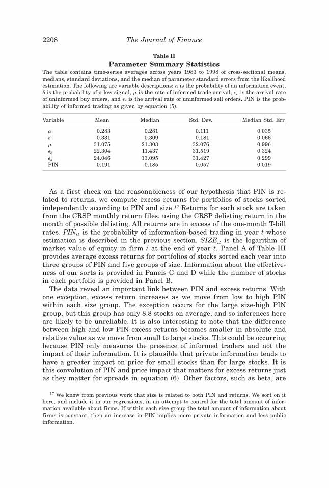
Given that the parameter estimates are stable across years, we pool theyears to further illustrate the distribution of the parameters across stocks.Figure 4 shows these pooled distributions for our estimated parameters, andTable II presents summary statistics. It is clear from the figure that thecomposite parameter PIN is rather tightly distributed around the mode 0.18,while a and, in particular, d, are more dispersed over the parameter space.The skewness of d is consistent with the generally rising stock prices overthis period; stocks typically did well, so the probability of bad news wasgenerally lower than that of good news. We have aggregated the uninformedtrading variables to depict the balance between uninformed buying and sell-ing. Over our time interval, uninformed traders were marginally more likelyto sell, while informed traders were more likely to buy. This, too, is consis-tent with the economic conditions of our sample, as informed traders werebetter able to capture the benefits of good news and thus rising stock prices.

In summary, we have been able to estimate our structural model for across section of stocks. The individual parameter estimates appear econom-ically reasonable, and the small standard errors of our estimates indicatestrong statistical significance. The time series of our estimates indicate aremarkable stability, with very little year-to-year movement in our esti-mated parameters. Our contention is that the estimated variables measurethe components of information-based trading, and their combination intoour PIN variable provides a concrete measure of this risk for each stock.

IV. Asset-Pricing Tests

A. Data and Methodology

For the asset-pricing tests, we need to use additional data on firm char-acteristics and returns. These data are available from the monthly CRSPfiles and the annual COMPUSTAT files. Data are not available for all of ourlisted firms, so the sample used in our asset-pricing tests is drawn from theintersection of the NYSE-listed firms on the CRSP and COMPUSTAT files.The monthly samples contain between 997 and 1,316 stocks for the period1984 to 1998, yielding 180 monthly observations to aggregate over time. Oneconcern we note at the outset is the length of our sample period. Asset-pricing tests typically employ long sample periods, but transaction data,which we need to calculate our PIN variable, are not available prior to 1983,and since we employ lagged PIN estimates, the asset-pricing tests begin in1984. Longer sample periods enhance the ability to find statistically signif-icant factors inf luencing returns, so our limited sample period imposes aparticularly stringent constraint on our testing approach.


Figure 4. Parameter distributions with pooled data. The figure shows the empiricaldistribution of the microstructure model parameters with all stocks and all years pooled.Panel A gives the distribution of a, the probability that an information event has occurred.Panel B shows the distribution for d, the probability of an information day containing bad news.~Figure continues on next page.!


Figure 4—continued. Parameter distributions with pooled data. Panel C contains thedistribution of PIN. Panel D shows the distribution of the uninformed order f low imbalance,~eb 2 es!0~eb 1 es!.


As a first check on the reasonableness of our hypothesis that PIN is re-lated to returns, we compute excess returns for portfolios of stocks sortedindependently according to PIN and size.17 Returns for each stock are takenfrom the CRSP monthly return files, using the CRSP delisting return in themonth of possible delisting. All returns are in excess of the one-month T-billrates. PINit is the probability of information-based trading in year t whoseestimation is described in the previous section. SIZEit is the logarithm ofmarket value of equity in firm i at the end of year t. Panel A of Table IIIprovides average excess returns for portfolios of stocks sorted each year intothree groups of PIN and five groups of size. Information about the effective-ness of our sorts is provided in Panels C and D while the number of stocksin each portfolio is provided in Panel B.

The data reveal an important link between PIN and excess returns. Withone exception, excess return increases as we move from low to high PINwithin each size group. The exception occurs for the large size-high PINgroup, but this group has only 8.8 stocks on average, and so inferences hereare likely to be unreliable. It is also interesting to note that the differencebetween high and low PIN excess returns becomes smaller in absolute andrelative value as we move from small to large stocks. This could be occurringbecause PIN only measures the presence of informed traders and not theimpact of their information. It is plausible that private information tends tohave a greater impact on price for small stocks than for large stocks. It isthis convolution of PIN and price impact that matters for excess returns justas they matter for spreads in equation ~6!. Other factors, such as beta, are

17 We know from previous work that size is related to both PIN and returns. We sort on ithere, and include it in our regressions, in an attempt to control for the total amount of infor-mation available about firms. If within each size group the total amount of information aboutfirms is constant, then an increase in PIN implies more private information and less publicinformation.

Table II

Parameter Summary StatisticsThe table contains time-series averages across years 1983 to 1998 of cross-sectional means,medians, standard deviations, and the median of parameter standard errors from the likelihoodestimation. The following are variable descriptions: a is the probability of an information event,d is the probability of a low signal, m is the rate of informed trade arrival, eb is the arrival rateof uninformed buy orders, and es is the arrival rate of uninformed sell orders. PIN is the prob-ability of informed trading as given by equation ~5!.

Variable Mean Median Std. Dev. Median Std. Err.

a 0.283 0.281 0.111 0.035d 0.331 0.309 0.181 0.066m 31.075 21.303 32.076 0.996eb 22.304 11.437 31.519 0.324es 24.046 13.095 31.427 0.299PIN 0.191 0.185 0.057 0.019


not controlled for in our portfolios, but these results do show that PIN isrelated to returns. Whether this relationship occurs because of the covari-ance of PIN and other factors is the question we address next by includingPIN in a standard asset-pricing regression.

To allow for comparability with previous work, our methodology followsthat of Fama and French ~1992!. Fama and French explored the determi-nants of the cross-sectional variation in returns and found that beta, size,and book-to-market ~i.e., the ratio of the book value of equity to the marketvalue of equity! all inf luenced returns. Consequently, we include these vari-ables, as well as our estimated PIN variable, in our analysis of asset-pricingreturns. We also explore whether the effect of PIN can be captured by pre-viously suggested proxies for liquidity, namely bid-ask spreads and shareturnover, or by return variation, by including these variables in the asset-pricing regressions.

We calculate betas using the following approach. Preranking portfolio be-tas are estimated for individual stocks using monthly returns from at leasttwo years to, when possible, five years, before the test year. Thus, for eachstock, we use at least 24 monthly return observations in the estimation. Weregress these stock returns on the contemporaneous and lagged value-weighted CRSP NYSE0AMEX index. Preranking portfolio betas are then given

Table III

Portfolio Excess ReturnsThe table contains results for portfolios of stocks sorted independently by size and PIN, wheresize is the market value of equity measured at the end of year t 2 1 and PIN is the probabilityof informed trading as given by equation ~5! estimated over year t 2 1. For each year, stocks aresorted into three PIN groups, ranging from low to high, and five size groups, ranging fromsmall to large. The reported results are averages of the relevant variables over the sampleperiod 1984 to 1998. Panel A reports average excess returns, Panel B reports the averagenumber of stocks in each portfolio, Panel C reports the average size in $ millions of the stocksin each portfolio, and Panel D reports the average PIN of stocks in each portfolio.

Size0PIN Low Medium High Size0PIN Low Medium High

Panel A: Excess Returns Panel B: Number of Stocks

Small 0.148 0.202 0.474 Small 21.9 60.1 142.52 0.462 0.556 0.743 2 30.5 79.0 115.73 0.647 0.695 0.892 3 54.4 95.5 75.14 0.873 0.837 0.928 4 93.4 99.0 32.7Large 0.953 1.000 0.643 Large 174.4 41.6 8.8

Panel C: Size Panel D: PIN

Small 75.3 79.4 71.2 Small 0.134 0.186 0.2572 257.6 257.3 244.6 2 0.138 0.186 0.2473 665.2 641.9 602.3 3 0.137 0.183 0.2374 1,719.1 1,593.6 1,473.9 4 0.138 0.180 0.231Large 9,845.7 4,439.9 4,814.3 Large 0.127 0.175 0.233


as the sum of the two coefficients ~this approach, suggested by Dimson ~1979!,is intended to correct for biases arising from nonsynchronous trading!. Next,40 portfolios are sorted every January on the basis of the estimated betas,and monthly portfolio returns are calculated as equal-weighted averages ofindividual stock returns. Postranking portfolio betas are estimated from thefull sample period, such that one beta estimate is obtained for each of the 40portfolios. Portfolio returns are regressed on contemporaneous and laggedvalues of CRSP index returns. The portfolio beta, Zbp, is then the sum of thetwo coefficients. We use individual stocks in the cross-sectional regressions,so individual stock betas are taken as the beta of the portfolio to which theybelong. Because the portfolio compositions change each year, individual stockbetas vary over time.

Book value of common equity is obtained from the annual COMPUSTATfiles ~item 60!. Following Fama–French, we exclude firms with negative bookvalues, and we set BE0ME values outside the 0.005 and 0.995 fractiles equalto these fractiles, respectively. We take logs, such that the explanatory vari-able, BMit21, is ln~BEt210MEt21! for firm i.

For each month in the sample period 1984 to 1998, we ran the followingcross-sectional regression:

Rit 5 g0t 1 g1t Zbp 1 g2t PINit21 1 g3t SIZEit21 1 g4t BMit21 1 hit , ~7!

where Rit is the excess return of stock i in month l of year t ~monthly sub-scripts omitted!, gjt , j 5 1, . . . ,5, are the estimated coefficients, and hit is themean-zero error term. The coefficients from the cross-sectional regressionsare averaged through time, using the standard Fama and MacBeth ~1973!methodology. Because this procedure is inefficient under time-varying vol-atility, we also use the correction technique suggested by Litzenberger andRamaswamy ~1979!. This correction weights the coefficients by their preci-sions when summing across the cross-sectional regressions, and is essen-tially a weighted least-square methodology. We report both the unadjustedand the Litzenberger–Ramaswamy adjusted coefficients.

A problem with almost all variables provided as alternatives to beta as theexplanatory variable of the cross section of returns ~e.g., size, book-to-market, earnings-to-price, turnover, etc.! is that these variables depend onthe security price. Miller and Scholes ~1982! noted that the inverse of pricemay be a good measure of the conditional beta, and therefore regressionanalysis may be capturing mismeasurement of beta, rather than some al-ternative priced factor. Berk ~1995! makes a related point. Because the es-timation of PIN involves only trades, we avoid this potential critique in ourinclusion of PIN.

Our primary interest lies in the time-series average of g2t , namely thecoefficient for PIN. Our hypothesis is that a higher risk of information-based trading for a stock translates into a higher required return for thatstock, so we expect a significantly positive average coefficient on PIN.


B. Results

Summary statistics on the variables in the asset-pricing regression areprovided in Table IV. The procedure on beta sorting portfolios results in areasonably broad variation in beta, with beta ranging between 0.52 and1.64. As noted in the previous section, our estimated PIN variable has amean of 0.19, while ranging from 0 to 0.53. The means of the size andbook-to-market variables are also consistent with prior work on this sam-ple period.

We first investigate the interrelationships of the explanatory variables,and in particular how PIN correlates with each variable. Table V presentstime-series means of the monthly bivariate correlations of the variables inthe asset-pricing tests. One of the largest absolute correlations is betweensize and PIN, with an average correlation of 20.58. This finding confirmsresults from earlier research that larger firms tend to have lower probabil-ities of informed trading. One might expect that stocks with greater privateinformation have higher systematic volatility, and this appears to be thecase: PIN is positively correlated with beta, with a correlation of 0.163. Wehad weaker priors on the relationship between PIN and BM, but note apositive correlation ~0.168!. The correlation between return and PIN is ratherlow, but the correlation between return and the other explanatory variablesis similarly low.

Table IV

Summary StatisticsThe table contains means, medians, minimum value, and maximum values on the variables in-cluded in the asset-pricing tests. All statistics are calculated from the full sample, that is, poolingall months. RETURN is the percentage monthly return in excess of the one-month T-bill rate.BETAs are portfolio betas estimated from the full period using 40 portfolios. PIN is the proba-bility of informed trading given by equation ~5! and estimated yearly for each stock. PPIN is theportfolio PIN calculated by first sorting all stocks into 40 portfolios according to PIN each year,and then taking the average within each portfolio of the individual stock PIN in the followingyear. SIZE is the logarithm of year-end market value of equity. BM is the logarithm of book valueof equity divided by market value of equity. SPREAD is the yearly average of the daily openingspreads of stock i. STD is the daily return standard deviation for stock i in year t. TURNOVERis the logarithm of the average monthly turnover year t 2 3 to t 2 1, and CVTURN is the logarithmof the coefficient of variation of the monthly turnover year t 2 3 to t 2 1.

Variable Mean Median Min. Max.

RETURN 0.73 0.47 2100.64 339.69BETA 1.09 1.09 0.52 1.64PIN 0.19 0.18 0.00 0.53PPIN 0.19 0.19 0.10 0.31SIZE 13.29 13.30 6.65 18.62BM 20.52 20.47 23.35 2.39SPREAD 1.52 1.14 0.14 15.07STD 2.10 1.88 0.46 14.92TURNOVER 1.56 1.59 22.33 4.37CVTURN 20.68 20.69 22.07 1.30


Return and beta are negatively correlated, but, as discussed below, this isin line with prior findings in this sample period. Likewise, the positive cor-relation between return and size is opposite of that reported in earlier pe-riods, but it is consistent with findings from our sample period. Finally, thelow correlation between return and BM is not unexpected given Loughran’s~1997! finding that book-to-market arises primarily in Nasdaq stocks, andour sample uses only NYSE firms.

The results from the asset-pricing tests are provided in Table VI. Theresults give striking evidence that the risk of informed trading as capturedby PIN is priced in the required returns of stocks. Looking at the weightedleast-squares results, we find a positive and significant coefficient on PIN~t-value 4.362!. The point estimate of the PIN coefficient has the naturalinterpretation that a difference of 10 percentage points in PIN between twostocks translates into a difference in required return of 0.21 percent permonth. This is an economically meaningful and significant difference. Wealso find a significant and positive coefficient on size ~t-value 9.994!, and asignificant, but negative, coefficient on beta ~t-value 26.22!. This latter find-ing, while inconsistent with standard asset-pricing theory, is consistent withthe findings of Fama and French ~1992!, Chalmers and Kadlec ~1998!, andDatar et al. ~1998!, who investigate similar sample periods. Book-to-marketis not significant, a finding not unexpected given our earlier discussion.

Table V

Simple CorrelationsThe table contains the time-series means of monthly bivariate correlations of the variables inthe asset-pricing tests. RETURN is the percentage monthly return in excess of the one-monthT-bill rate. BETAs are portfolio betas estimated from the full period using 40 portfolios. PIN isthe probability of informed trading given by equation ~5! and estimated yearly for each stock.PPIN is the portfolio PIN calculated by first sorting all stocks into 40 portfolios according toPIN each year, and then taking the average within each portfolio of the individual stock PIN inthe following year. SIZE is the logarithm of year-end market value of equity. BM is the loga-rithm of book value of equity divided by market value of equity. SPREAD is the yearly averageof the daily opening spreads of stock i. STD is the daily return standard deviation for stock iin year t. TURNOVER is the logarithm of the average monthly turnover year t 2 3 to t 2 1,and CVTURN is the logarithm of the coefficient of variation of the monthly turnover year t 2 3to t 2 1.

BETA PIN SIZE BM SPREAD STD TURNOVER CVTURN PPIN

RETURN 20.015 20.006 0.023 20.005 20.022 20.038 20.021 20.019 20.008BETA 0.163 20.207 0.009 0.222 0.434 0.294 0.089 0.171PIN 20.576 0.168 0.353 0.239 20.187 0.412 0.572SIZE 20.384 20.708 20.493 0.123 20.547 20.568BM 0.273 0.112 20.030 0.160 0.162SPREAD 0.748 20.116 0.397 0.328STD 0.294 0.331 0.236TURNOVER 20.006 20.169CVTURN 0.397


That PIN affects asset returns is consistent with the economic analysismotivating our work. We believe that the PIN variable captures aspects ofthe dynamic efficiency of stock prices. These dynamic effects arise becauseinformation-based trading affects not only the spread, but the evolution ofprices as well. Our results are consistent with this dynamic efficiency in-f luencing the required returns for stocks.

C. Potential Errors in Variables for PIN

PIN, just like beta, is an estimated variable, and so it is potentially sub-ject to an errors-in-variables ~EIV! bias. This difficulty has long been recog-nized in beta estimation, and the portfolio approach of Fama and French isdesigned to correct for this problem. In effect, the solution is to create aninstrumental variable to use in place of the variable in question. Assumingthat the EIV problem has been corrected for beta, the only variable in equa-tion ~7! measured with potential errors is PIN. In this case, the bias on thecoefficient on PIN is unambiguously downward; hence the bias is againstfinding any effect of PIN. However, we have done a portfolio construction forPIN similar to that of beta. Thus, a simple test for the importance of thisproblem is to see if our estimated PIN coefficients change when we use thisportfolio approach.

Forty portfolios are sorted each year, t 2 2, on the basis of the estimatedPINs. The portfolio PIN is then the average of the estimated PINs for theyear t 2 1, and this variable, PPIN, is then assigned to each stock in theportfolio. This technique is meant to ensure that the error in PPIN is un-correlated with the error term. The instrument should also be highly correlatedwith the original variable. Table V shows that the average cross-sectionalcorrelation between PIN and PPIN is 0.572. We then run the same cross-sectional regression, now using these portfolio PINs. The results are pro-

Table VI

Asset-Pricing TestsThe table contains time-series averages of the coefficients in cross-sectional asset-pricing testsusing standard Fama and MacBeth ~1973! methodology and Litzenberger and Ramaswamy~L-R; 1979! precision-weighted means ~weighted least-squares ~WLS!!. The dependent variableis the percentage monthly return in excess of the one-month T-bill rate. BETAs are portfoliobetas calculated from the full period using 40 portfolios. PIN is the probability of information-based trading in stock i of year t 2 1. SIZE is the logarithm of market value of equity ~ME! infirm i at the end of year t 2 1, and BM is the logarithm of the ratio of book value of commonequity to market value of equity for firm i in year t 2 1. T-values are given in parentheses.

Beta PIN SIZE BM

Fama–MacBeth 20.175 1.800 0.161 0.051~20.481! ~2.496! ~2.808! ~0.480!

L-R WLS 20.482 2.086 0.168 0.042~26.22! ~4.362! ~9.994! ~1.120!


vided in the upper half of Table VII. The coefficients on PPIN are very closeto the coefficients on PIN in Table VI, but the t-values are substantiallyreduced. PPIN remains significant only in the weighted least-squares re-gression where the coefficient on PPIN is 2.40 with a t-value of 2.717.

The insignificant change in the coefficient on PIN and the reduced t-valuessuggest that, though it may be correcting for an EIV problem, the portfolioapproach primarily adds noise to the PIN variable. In a single regressionframework, a test for EIV is to include both the instrument and the originalvariable in the regression. If there is an EIV problem, and the instrumentfixes it, then the coefficient on the original variable should be zero, while ifthere is not an EIV problem, then the coefficient on the instrument would bezero. Therefore, we included both PPIN and PIN in the regressions, and theresults are reported in the bottom half of Table VII. In this case, the coef-ficient on PIN is not significantly different from the result of the regressionexcluding PPIN. The coefficient on PPIN, however, is not significantly dif-ferent from zero. This strongly suggests that the portfolio approach appliedto PIN does not correct for any EIV problem. Thus we focus our discussionon regressions using PIN rather than the instrument PPIN.

D. Alternative Explanations

It is natural to ask whether PIN works in our asset-pricing regressionsbecause it is a fundamental priced variable, or because it is serving as aproxy for some omitted variable. There are three obvious candidates, and

Table VII

Errors in VariablesThe table contains time-series averages of the coefficients in cross-sectional asset-pricing testsusing standard Fama and MacBeth ~1973! methodology and Litzenberger and Ramaswamy~L-R; 1979! precision-weighted means. The dependent variable is the percentage monthly re-turn in excess of the one-month T-bill rate. Betas are portfolio betas calculated from the fullperiod using 40 portfolios. PIN is the probability of information-based trading in stock i of yeart 2 1. PPIN is the portfolio pin calculated by first sorting all stocks into 40 portfolios accordingto PIN each year, and then taking the average within each portfolio of the individual stock PINin the following year. SIZE is the logarithm of market value of equity ~ME ! in firm i at the endof year t 2 1, and BM is the logarithm of the ratio of book value of common equity to marketvalue of equity for firm i in year t 2 1. T-values are given in parentheses.

Beta PIN PPIN SIZE BM

Fama–MacBeth 0.022 1.882 0.143 0.010~0.058! ~1.435! ~2.399! ~0.096!

L-R WLS 20.290 2.400 0.152 20.001~23.52! ~2.717! ~8.629! ~20.016!

Fama–MacBeth 0.013 1.758 0.813 0.167 0.013~0.035! ~2.362! ~0.647! ~2.703! ~0.121!

L-R WLS 20.298 1.940 1.174 0.179 0.001~23.60! ~3.561! ~1.241! ~9.394! ~0.019!


innumerable less obvious candidates, for the omitted variable designation.The most obvious candidate is spreads. Earlier researchers ~e.g., Amihudand Mendelson ~1986!! found a positive relationship between spread andreturns, so it could be that PIN is serving as a proxy for spread. Second, astock with a high PIN is one with substantial imbalances in trades, and thusis a stock whose price is likely to be highly variable.18 So it could be that PINis serving as a proxy for the variability of returns on the stock. Of course, tothe extent that this risk can be diversified away, it should not be priced, andany nondiversifiable component of the risk should be picked up by b. But weknow that CAPM does not work well over this time period, so this risk couldbe positively related to observed average excess returns.19 Finally, there hasbeen substantial interest in the role of volume, or turnover, in explainingasset-price behavior. Therefore, we test whether PIN is merely serving as aproxy for these measures. We consider each of these variables in turn, andwhile we show that they are correlated with PIN as expected, we also showthat when they are included in the returns regression they do not eliminatethe direct effect of PIN. Results of the regressions are reported in Table VIII.

We first consider the bid-ask spread. We define the variable SPREADit21to be the average of the daily opening percentage spreads for firm i in yeart 2 1. We know from Table V that PIN and SPREAD are positively, but notperfectly, correlated. Indeed, the correlation is a relatively low 0.353, ref lect-ing that spreads can be affected by many factors other than information. IsPIN or SPREAD the better predictor of returns? We test this by first in-cluding SPREAD in place of PIN in the asset-pricing regression and thenby including both SPREAD and PIN in the regression. When SPREADis included, and PIN is excluded, SPREAD is insignificant in the Fama–MacBeth regression, while it is significantly negative in the weighted least-squares regression. This result is not what would be expected from liquidity-based theories of asset returns. When SPREAD and PIN are both included,PIN remains highly significant ~t-value 5 3.88! with the correct positivesign. The inclusion of spread reduces the coefficient on PIN only slightlyfrom 2.09 to 1.87.

That it is PIN, and not SPREAD, that affects asset-pricing returns is con-sistent with the economic analysis motivating our work. While traders un-doubtedly care about spreads, they are more concerned with the risk of holdingthe stock, and this is affected by the extent of private information. Information-based trading does give rise to spreads, but spreads in actual markets can be

18 This relationship is not completely straightforward because although trade moves prices,public information events, which in our model do not generate trade, also move prices. So therecould be stocks with low PIN, that is little information-based trade, and highly variable pricescaused by the release of public information. This is consistent with our analysis in that publicevents can move the range of true values of the stock.

19 Note that our theoretical model ~equation ~6!! includes essentially a standard deviationterm as it measures the losses due to the risk of informed trading. Thus, it seems reasonablethat PIN and standard deviation could both play a role due to risk. We thank the referee forraising this point.


affected by many other factors such as minimum tick sizes, specialist con-tinuity rules, and even market power. These factors dictate that spreadswill be, at best, a noisy proxy for the risk of informed trading. PIN is alsoa proxy for the risk of informed trading, and as it is estimated from tradedata, it too could be inf luenced by the factors listed above. But our results

Table VIII

Alternative ExplanationsThe table contains time-series averages of the coefficients in cross-sectional asset-pricing testsusing standard Fama and MacBeth ~1973! methodology and Litzenberger and Ramaswamy~L-R; 1979! precision-weighted means. The dependent variable is the percentage monthly re-turn in excess of the one-month T-bill rate. Betas are portfolio betas calculated from the fullperiod using 40 portfolios. PIN is the probability of information-based trading in stock i of yeart 2 1. SIZE is the logarithm of market value of equity ~ME! in firm i at the end of year t 2 1,and BM is the logarithm of the ratio of book value of common equity to market value of equityfor firm i in year t 2 1. SPREAD is the average daily opening percentage spread for firm i inyear t 2 1. STD is the standard deviation of daily returns for firm i in year t 2 1. TURNOVERis the logarithm of the average monthly turnover year t 2 3 to t 2 1, and CVTURN is thelogarithm of the coefficient of variation of the monthly turnover year t 2 3 to t 2 1. T-values aregiven in parentheses.

Beta PIN SIZE BM SPREAD STD TURNOVER CVTURN

Fama–MacBeth 20.146 0.106 0.037 20.060~20.407! ~2.122! ~0.353! ~20.745!

L-R WLS 20.425 0.081 0.035 20.060~25.47! ~4.333! ~0.930! ~22.66!

Fama–MacBeth 20.164 1.694 0.144 0.044 20.052~20.458! ~2.483! ~2.849! ~0.419! ~20.650!

L-R WLS 20.441 1.866 0.124 0.041 20.051~25.66! ~3.882! ~5.746! ~1.100! ~22.27!

Fama–MacBeth 0.159 0.053 20.009 20.318~0.486! ~1.138! ~20.088! ~22.73!

L-R WLS 0.008 0.034 20.016 20.354~0.102! ~2.172! ~20.416! ~213.0!

Fama–MacBeth 0.141 1.411 0.084 20.002 20.311~0.435! ~2.104! ~1.748! ~20.024! ~22.67!

L-R WLS 20.008 1.405 0.064 20.010 20.345~20.100! ~2.932! ~3.458! ~20.271! ~212.6!

Fama–MacBeth 0.047 0.119 0.051 20.305 20.210~0.144! ~2.166! ~0.486! ~23.27! ~22.44!

L-R WLS 20.237 0.134 0.046 20.336 20.178~22.88! ~7.762! ~1.222! ~29.95! ~22.73!

Fama–MacBeth 0.025 1.328 0.139 0.054 20.288 20.242~0.077! ~1.718! ~2.444! ~0.519! ~22.99! ~22.86!

L-R WLS 20.260 1.454 0.156 0.048 20.315 20.214~23.14! ~2.956! ~8.306! ~1.276! ~29.17! ~23.23!

Fama–MacBeth 0.276 1.415 0.133 20.019 0.203 20.466 20.072 20.193~0.939! ~2.005! ~2.694! ~20.190! ~2.179! ~23.38! ~20.927! ~22.15!

L-R WLS 0.107 1.350 0.121 20.018 0.198 20.489 20.090 20.159~1.225! ~2.723! ~5.274! ~20.485! ~5.724! ~211.2! ~22.19! ~22.39!


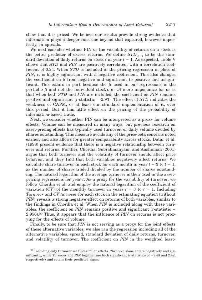
show that it is priced. We believe our results provide strong evidence thatinformation plays a deeper role, one beyond that captured, however imper-fectly, in spreads.

We next consider whether PIN or the variability of returns on a stock isthe better predictor of excess returns. We define STDit21 to be the stan-dard deviation of daily returns on stock i in year t 2 1. As expected, Table Vshows that STD and PIN are positively correlated, with a correlation coef-ficient of 0.24. When STD is included in the pricing regression in place ofPIN, it is highly significant with a negative coefficient. This also changesthe coefficient on b from negative and significant to positive and insigni-ficant. This occurs in part because the b used in our regressions is theportfolio b and not the individual stock’s b. Of more importance for us isthat when both STD and PIN are included, the coefficient on PIN remainspositive and significant ~t-statistic 5 2.93!. The effect of STD indicates theweakness of CAPM, or at least our standard implementation of it, overthis period. But it has little effect on the pricing of the probability ofinformation-based trade.

Next, we consider whether PIN can be interpreted as a proxy for volumeeffects. Volume can be measured in many ways, but previous research onasset-pricing effects has typically used turnover, or daily volume divided byshares outstanding. This measure avoids any of the price-beta concerns notedearlier, and also allows for greater comparability across stocks. Datar et al.~1998! present evidence that there is a negative relationship between turn-over and returns. Further, Chordia, Subrahmanyam, and Anshuman ~2001!argue that both turnover and the volatility of turnover should affect pricebehavior, and they find that both variables negatively affect returns. Wecalculate share turnover in each stock for each month in year t 2 3 to t 2 1,as the number of shares traded divided by the number of shares outstand-ing. The natural logarithm of the average turnover is then used in the asset-pricing regressions for year t. As a proxy for the variability of turnover, wefollow Chordia et al. and employ the natural logarithm of the coefficient ofvariation ~CV! of the monthly turnover in years t 2 3 to t 2 1. IncludingTurnover and CV turnover for each stock in the estimating equation ~withoutPIN! reveals a strong negative effect on returns of both variables, similar tothe findings in Chordia et al. When PIN is included along with these vari-ables, the coefficient on PIN remains positive and significant ~t-statistic 52.956!.20 Thus, it appears that the inf luence of PIN on returns is not prox-ying for the effects of volume.

Finally, to be sure that PIN is not serving as a proxy for the joint effectsof these alternative variables, we also ran the regression including all of thealternative variables, spread, standard deviation of daily returns, turnover,and volatility of turnover. The coefficient on PIN in the weighted least-

20 Including only turnover we find similar effects. Turnover alone enters negatively and sig-nificantly, while Turnover and PIN together are both significant ~t-statistics of 29.88 and 2.42,respectively! and retain their predicted signs.


squares ~WLS! regression is 1.35 with a t-statistic of 2.723. Thus PIN is notproxying for the joint effect of these alternative variables. It is also worthnoting from the regression that spread now is positive and significant. Theinclusion of the standard deviation of returns is important for this result,suggesting that the underlying asset pricing model may be mis-specified.

In summary, the positive relationship between expected return and theprobability of informed trading seems be to robust to the inclusion of differ-ent explanatory variables in the cross-sectional regressions. Thus, there isevidence that the risk of informed trading is, indeed, an important determi-nant of required stock returns.

V. Conclusions

We have investigated the role of information-based trading in affectingasset returns. Our premise is that in a dynamic market, asset prices arecontinually adjusting to new information. This evolution dictates that theprocess by which asset prices become informationally efficient cannot beseparated from the process generating asset returns. Our theoretical modelsuggests that private information inf luences this price evolution, and in sodoing, affects the risk of holding the asset. We investigate this link betweenasset prices and private information by using the structure of a sequentialtrade market microstructure model to derive an explicit measure of the prob-ability of information-based trading for an individual stock. We then esti-mate this probability for a large sample of NYSE-listed stocks. Incorporatingour probability estimates into a standard asset-pricing framework revealedstrong support for our hypothesis: Information-based trading has a largeand significantly positive effect on asset returns. Indeed, our estimated in-formation variable and firm size are the predominant factors explainingreturns.

That the risk of information-based trading affects asset returns raises ahost of important questions regarding asset pricing in general, and asset-pricing models in particular. Brevity precludes addressing all of these, butwe do feel it useful to consider three general issues. These involve the theo-retical basis for our result, the empirical properties of PIN, and the impli-cations of our results for future research.

Of particular importance is why this can occur in a seemingly efficientcapital market. A natural objection to all candidates put forward to explainasset returns is that, with the exception of systematic risk, the actions ofarbitrageurs should remove any such proposed influence on the market. Whilethis may be accurate for some factors, we do not believe that it is accuratewith respect to asymmetric information. In a world with asymmetric infor-mation, an uninformed investor is always at a disadvantage relative to trad-ers with better information. In bad times, this disadvantage can result inthe uninformed trader’s portfolio holding too much of the stock; in good times,the trader’s portfolio has too little of the stock. Holding many stocks cannot


remove this effect because the uninformed do not know the proper weightsof each asset to hold. In this sense, asymmetric information risk is system-atic because, like market risk, it cannot be diversified away.21

In our empirical work we found that PIN, the probability of information-based trading variable, actually dominated all other variables, including b,in explaining returns. Given our argument that information has a system-atic component, this should not be unexpected. We caution, however, thatour results do not mean that only private information matters in asset pric-ing. What our results do suggest is that the effects of information may bemore pervasive, and important, than our simple theories, and asset-pricingmodels, have thus far considered.

The success of our PIN variable naturally leads to questions regarding itsempirical properties. A very useful exercise would be to examine the cross-sectional determinants of PIN, and in particular how PIN relates to vari-ables such as industry or accounting measures. Not surprisingly, this is alarge endeavor and one we hope to address in future work. One benefit ofsuch a project could be to determine a set of “sufficient statistics” for PINthat involves accounting data. As is clear from this paper, the actual calcu-lation of PIN requires a tremendous amount of computation. ReplicatingPIN with more easily available data would make it easier to apply, andwould have the added benefit of explaining why it is that some accountingdata appears to be informative for asset pricing.

Finally, our results here suggest a number of directions for future re-search. Our results suggest that a firm could lower its cost of capital if itcould reduce its PIN. Public disclosure of information that would otherwisebe private could do this. Botosan ~1997! provides support for this idea byshowing that for a sample of firms with low analyst following greater dis-closure of information reduces the cost of capital by an average of 28 basispoints. There is now a substantial body of work suggesting that volume, andvolume-linked variables, play an important role in asset pricing. We haveshown here that PIN is not a volume effect, but there remains the intriguingquestion of whether volume effects may not be proxying for some of theunderlying components of PIN, such as the rate of uninformed trade or theprobability of new information. Investigating the role of the components ofPIN would provide insight into this issue. An equally intriguing issue ismomentum. There is now widespread, if in some cases grudging, acceptanceof the fact that momentum affects asset prices. These momentum effectsappear to arise over relatively short time intervals ~months 3–12!, and theypose a challenge for virtually all asset-pricing theories. One possible expla-nation is that momentum is somehow linked to the underlying information

21 It is also not the case in our model that the informed traders will simply trade the effectaway because they too face risk in holding the asset. Informed traders are also risk averse, andso there will always be a premium to hold the risky asset. However, because the stock is rel-atively less risky for the informed, in equilibrium, their expected holdings of the asset exceedthat of the uninformed ~see Easley and O’Hara ~2000! for more analysis and discussion!.


structure of the stock. Testing for such effects using our approach wouldrequire finer estimates ~i.e., monthly! of our PIN variable, as well as poten-tially a longer time frame. We hope to consider this in future research.

REFERENCES

Admati, Anat, 1985, A noisy rational expectations equilibrium for multi-asset securities mar-kets, Econometrica 53, 629–658.

Amihud, Yakov, 2000, Illiquidity and stock returns: Cross-sectional and time series effects, Work-ing paper, New York University.

Amihud, Yakov, and Haim Mendelson, 1986, Asset pricing and the bid-ask spread, Journal ofFinancial Economics 17, 223–249.

Amihud, Yakov, and Haim Mendelson, 1989, The effects of beta, bid-ask spread, residual risk,and size on stock returns, Journal of Finance 44, 479–486.

Amihud, Yakov, Haim Mendelson, and B. Lauterbach, 1997, Market microstructure and secu-rities values: Evidence from the Tel Aviv Stock Exchange, Journal of Financial Economics45, 365–390.

Barry, Christopher B., and Stephen J. Brown, 1984, Differential information and the small firmeffect, Journal of Financial Economics 13, 283–294.

Barry, Christopher B., and Stephen J. Brown, 1985, Differential information and security mar-ket equilibrium, Journal of Financial Quantitative Analysis 20, 407–422.

Barry, Christopher B., and Robert H. Jennings, 1992, Information and diversity of analystopinion, Journal of Financial and Quantitative Analysis 27, 169–183.

Basak, Suleyman, and Domenico Cuoco, 1998, An equilibrium model with restricted stock mar-ket participation, Review of Financial Studies 11, 309–341.

Berk, Jonathan B., 1995, A critique of size-related anomalies, Review of Financial Studies 8,275–286.

Botosan, Caval A., 1997, Disclosure level and the cost of equity capital, The Accounting Review72, 323–349.

Brennan, Michael J., and Henry H. Cao, 1997, International portfolio investment f lows, Jour-nal of Finance 52, 1851–1880.

Brennan, Michael J., Tarun Chordia, and Avanidhar Subrahmanyam, 1998, Alternative factorspecifications, security characteristics, and the cross-section of expected stock returns, Jour-nal of Financial Economics 49, 345–373.

Brennan, Michael J., and Avanidhar Subrahmanyam, 1996, Market microstructure and assetpricing: On the compensation for illiquidity in stock returns, Journal of Financial Econom-ics 41, 441–464.

Chalmers, J.M., and Gregory B. Kadlec, 1998, An empirical examination of the amortized spread,Journal of Financial Economics 48, 159–188.

Chen, Nai-fu F., and Raymond Kan, 1996, Expected return and the bid-ask spread, in K.S.S.Saitou and K. Kubota, eds.: Modern Portfolio Theory and Applications ~Gakujutsu ShuppanCenter, Osaka, Japan!.

Chordia, Tarun, Avanidhar Subrahmanyam, and V.R. Anshuman, 2001, Trading activity andexpected stock returns, Journal of Financial Economics 59, 3–32.

Coles, Jeffrey L., Uri Loewenstein, and J. Suay, 1995, On equilibrium pricing under parameteruncertainty, Journal of Financial and Quantitative Analysis 30, 347–364.

Datar, V., Narayan Naik, and R. Radcliffe, 1998, Liquidity and stock returns: An alternativetest, Journal of Financial Markets 1, 203–219.

Dimson, Elroy, 1979, Risk measurement when shares are subject to infrequent trading, Journalof Financial Economics 7, 197—226.

Easley, David, Nicholas M. Kiefer, and Maureen O’Hara, 1996a, Cream-skimming or profit-sharing? The curious role of purchased order f low, Journal of Finance 51, 811–833.

Easley, David, Nicholas M. Kiefer, and Maureen O’Hara, 1997a, The information content of thetrading process, Journal of Empirical Finance 4, 159–186.


Easley, David, Nicholas M. Kiefer, and Maureen O’Hara, 1997b, One day in the life of a verycommon stock, Review of Financial Studies 10, 805–835.

Easley, David, Nicholas M. Kiefer, Maureen O’Hara, and Joseph Paperman, 1996b, Liquidity,information, and less-frequently traded stocks, Journal of Finance 51, 1405–1436.

Easley, David, and Maureen O’Hara, 2000, Information and the cost of capital, Working paper,Johnson Graduate School of Management, Cornell University.

Easley, David, Maureen O’Hara, and Joseph Paperman, 1998, Financial analysts and information-based trade, Journal of Financial Markets 1, 175—201.

Easley, David, Maureen O’Hara, and Gideon Saar, 2001, How stock splits affect trading: Amicrostructure approach, Journal of Financial and Quantitative Analysis 36, 25–51.

Eleswarapu, V.R., 1997, Cost of transacting and expected returns in the Nasdaq market, Jour-nal of Finance 52, 2113–2127.

Eleswarapu, V.R., and Marc R. Reinganum, 1993, The seasonal behavior of liquidity premiumin asset pricing, Journal of Financial Economics 34, 373–386.

Ellis, Katrina, Roni Michaely, and Maureen O’Hara, 2000, The accuracy of trade classificationrules: Evidence from Nasdaq, Journal of Financial and Quantitative Analysis 35, 529–551.

Fama, Eugene F., and Kenneth R. French, 1992, The cross section of expected stock returns,Journal of Finance 47, 427–465.

Fama, Eugene F., and James D. MacBeth, 1973, Risk, return, and equilibrium: Empirical tests,Journal of Political Economy 81, 607–636.

Grossman, Sanford, and Joseph Stiglitz, 1980, On the impossibility of informationally efficientmarkets, American Economic Review 70, 393–408.

Jones, Charles M., Gautam Kaul, Marc L. Lipson, 1994, Transactions, volume, and volatility,Review of Financial Studies 7, 631–651.

Jones, Charles M., and Steven L. Slezak, 1999, The theoretical implications of asymmetricinformation on the dynamic and cross-sectional characteristics of asset returns, Workingpaper, University of North Carolina, Chapel Hill.

Kyle, Albert S., 1985, Continuous auctions and insider trading, Econometrica 53, 1315–1335.Lee, Charles M.C., and Mark J. Ready, 1991, Inferring trade direction from intraday data,

Journal of Finance 46, 733–746.Lintner, John, 1969, The aggregation of investor ’s diverse judgments and preferences in purely

competitive security markets, Journal of Financial and Quantitative Analysis 4, 347–400.Litzenberger, Robert, and Krishna Ramaswamy, 1979, The effect of personal taxes and divi-

dends on capital asset prices: Theory and empirical evidence, Journal of Financial Eco-nomics 7, 163–196.

Loughran, Timothy, 1997, Book-to-market across firm size, exchange, and seasonality: Is therean effect? Journal of Financial and Quantitative Analysis 32, 249–268.

Merton, Robert C., 1986, A simple model of capital market equilibrium with incomplete infor-mation, Journal of Finance 42, 483–510.

Miller, Merton H., and Myron S. Scholes, 1982, Dividends and taxes: Some empirical evidence,Journal of Political Economy 90, 1118–1141.

O’Hara, Maureen, 1995, Market Microstructure Theory ~Blackwell Publishers, Cambridge, MA!.Shapiro, Alexander, 2001, The investor recognition hypothesis in a dynamic general equilib-

rium: Theory and evidence, Review of Financial Studies 15, 97–145.Wang, Jiang, 1993, A model of intertemporal asset prices under asymmetric information, Re-

view of Economic Studies 60, 249–282.


Is Information Risk a Determinant of Asset Returns? · rational expectations equilibrium to...

Documents

Transcript of Is Information Risk a Determinant of Asset Returns? · rational expectations equilibrium to...