University of Pennsylvania University of Pennsylvania

ScholarlyCommons ScholarlyCommons

Marketing Papers Wharton Faculty Research

11-30-2016

Is Dynamic Competition Socially Beneficial? The Case of Price as Is Dynamic Competition Socially Beneficial? The Case of Price as

Investment Investment

David Besanko

Ulrich Doraszelski University of Pennsylvania

Yaroslav Kryukov

Follow this and additional works at: https://repository.upenn.edu/marketing_papers

Part of the Behavioral Economics Commons, Business Administration, Management, and Operations

Commons, Business Intelligence Commons, Marketing Commons, and the Sales and Merchandising

Commons

Recommended Citation Recommended Citation Besanko, D., Doraszelski, U., & Kryukov, Y. (2016). Is Dynamic Competition Socially Beneficial? The Case of Price as Investment. Retrieved from https://repository.upenn.edu/marketing_papers/325

This is an unpublished manuscript.

This paper is posted at ScholarlyCommons. https://repository.upenn.edu/marketing_papers/325 For more information, please contact repository@pobox.upenn.edu.

Is Dynamic Competition Socially Beneficial? The Case of Price as Investment Is Dynamic Competition Socially Beneficial? The Case of Price as Investment

Abstract Abstract We study industries where prices are not limited to their allocative and distributive roles, but also serve as an investment into lower costs or higher demand. While our model focuses on learning-by-doing and the cost advantage that it implies, our conclusions also apply to industries driven by network externalities. Existing literature does not have a clear verdict on whether the investment role of prices benefits or hurts the overall welfare, as there are a number of economic forces at work, e.g. motivation to move down the learning curve faster could be offset by the ease of driving a weaker rival out of the market. We compute both market equilibrium and first-best solution. The resulting deadweight loss appears small, in the sense that eliminating the investment motive from pricing decisions leads to much worse outcomes. Further investigation into components of deadweight loss shows that while pricing distortions are the most important driver of the deadweight loss, these distortions can be fairly small. Entry-exit distortions that arise from duplicated set-up and fixed opportunity costs also contribute to the deadweight loss, but these distortions are partially offset by more beneficial industry structure, as the market equilibrium tends to result in more active firms than the first-best solution.

Disciplines Disciplines Behavioral Economics | Business | Business Administration, Management, and Operations | Business Intelligence | Marketing | Sales and Merchandising

Comments Comments This is an unpublished manuscript.

This working paper is available at ScholarlyCommons: https://repository.upenn.edu/marketing_papers/325

Is Dynamic Competition Socially Beneficial? The Case of

Price as Investment∗

David Besanko† Ulrich Doraszelski‡ Yaroslav Kryukov§

November 30, 2016

— Preliminary and Incomplete. Do not cite. —

Abstract

We study industries where prices are not limited to their allocative and distributiveroles, but also serve as an investment into lower costs or higher demand. While our modelfocuses on learning-by-doing and the cost advantage that it implies, our conclusions alsoapply to industries driven by network externalities. Existing literature does not havea clear verdict on whether the investment role of prices benefits or hurts the overallwelfare, as there are a number of economic forces at work, e.g. motivation to move downthe learning curve faster could be offset by the ease of driving a weaker rival out of themarket. We compute both market equilibrium and first-best solution. The resultingdeadweight loss appears small, in the sense that eliminating the investment motive frompricing decisions leads to much worse outcomes. Further investigation into components ofdeadweight loss shows that while pricing distortions are the most important driver of thedeadweight loss, these distortions can be fairly small. Entry-exit distortions that arisefrom duplicated set-up and fixed opportunity costs also contribute to the deadweightloss, but these distortions are partially offset by more beneficial industry structure, asthe market equilibrium tends to result in more active firms than the first-best solution.

1 Introduction

In perfectly competitive markets, prices play two roles: allocative and distributive. Pricesserve as incentive devices that shape how scarce resources are allocated within and acrossmarkets. Prices are also transfers between buyers and sellers, thus determining the distribu-tion of consumer and producer surplus. Prices play these same roles when firms have marketpower, but the distributive and allocative roles are typically in tension with each other inthis case.

∗We thank Guy Arie, Ariel Pakes, Robert Porter, Michael Raith, Mike Riordan, and Mike Whinston forhelpful discussions and suggestions. We also thank participants at seminars at Carnegie Mellon University,DG Comp at the European Commission, Helsinki Center for Economic Research, Johns Hopkins University,Toulouse School of Economics, Tulane University, and University of Rochester for their useful questions andcomments.

†Kellogg School of Management, Northwestern University, Evanston, IL 60208, d-besanko@kellogg.northwestern.edu.

‡Wharton School, University of Pennsylvania, Philadelphia, PA 19104, doraszelski@wharton.upenn.edu.§Tepper School of Business, Carnegie Mellon University, Pittsburgh, PA 15213, kryukov@cmu.edu.

1

In many interesting settings, though, there is third role for prices: investment. Theinvestment role arises when firms jostle for competitive advantage through the prices theyset. Examples include competition to build cumulative experience on a learning curve orcustomer base in markets with network effects, switching costs, or brand loyalty. In thesesituations, competition is dynamic as current demand translates into lower cost or higherdemand in the future, which in turn implies that current prices determine the future evolutionof market structure.1 Settings in which firms jostle for advantage through pricing are afeature of both “new economy” industries (e.g., Amazon versus Barnes and Noble in e-bookreaders or Sony versus Microsoft in gaming consoles) and “old economy” industries (e.g.,airframes, where each new generation of aircraft entails a learning curve).

In their review of the literature on network effects and switching costs, Farrell & Klem-perer (2007) point out that the investment role of prices opens up a second dimension ofcompetition, namely competition for the market:

For a firm, it makes market share a valuable asset, and encourages a com-petitive focus on affecting expectations and on signing up pivotal (notably early)customers, which is reflected in strategies such as penetration pricing; competi-tion is shifted from textbook competition in the market to a form of Schumpeteriancompetition for the market in which firms struggle for dominance.

The central question of this paper is whether this dynamic competition is socially beneficial.At first glance, it seems obvious that dynamic competition for advantage based on a

valuable asset such as cumulative know-how or installed base, even involving just a fewfirms, would be extremely efficient. This point can be made by drawing a contrast withrent-seeking models. In rent-seeking models firms compete for dominant market positionby engaging in socially wasteful activities (e.g., lobbying). In settings where price serves asan investment, firms also compete for dominant market position, but not through sociallywasteful activities. Instead they do it by transferring surplus to consumers through low prices(as they engage in competition for the market) and by creating positive social value through,for example, the generation of demand-side economies of scale or learning economies. Theremay indeed be some distortions due to deviations from first-best pricing, but we wouldexpect that these would be minimal in light of the investment value created by competition.

Though compelling, this intuition is incomplete. First, just because the investment roleof prices leads to prices that are less than static equilibrium prices does not imply that dead-weight losses (DWLs) will be lessened relative to a static setting. Pricing to gain advantagecould lead to periods in which prices are less than first-best prices, resulting in a DWL fromoverproduction. Second, when firms use price to jostle for advantage, Besanko et al. (2014)show that firms have an advantage-denying motive—they choose low prices (in part) to slowthe pace at which rivals build their advantages and perhaps make it more likely that theyexit the industry. This motive can give rise to equilibria with predation-like behavior andlong-run market structures involving monopolization by a single firm. Monopolization could,of course, lead to long-run distortions due to monopoly pricing, but it could also lead to wel-fare losses from insufficient product variety when consumers have a taste for variety. Third,

1Some models of non-price competition have a similar structure; see Besanko, Doraszelski & Kryukov(2014) for details and a list of these models.

2

even though competition for dominant market position when price serves as an investmentdoes not involve socially wasteful expenditures on activities such as lobbying, it could lead todistortions in entry conduct analogous to the coordination breakdowns in natural monopolymarkets highlighted in Bolton & Farrell (1990) or distortions in exit conduct due to war ofattrition dynamics (Maynard Smith 1974, Tirole 1988, Bulow & Klemperer 1999).

The question of whether imperfect competition comes close to achieving first-best welfarelevels when price has an investment role does not seem to have an “obvious” answer. Thegoal of this paper is to answer this question. We do so by analyzing a model of learning-by-doing along the lines of Cabral & Riordan (1994), Besanko, Doraszelski, Kryukov &Satterthwaite (2010), and Besanko et al. (2014) (hereafter BDK) that involves dynamicpricing competition in a differentiated product market with entry and exit. We computeMarkov perfect equilibria (MPE) and compare them to the solution to a social planner’sfirst-best (FB) problem in which the planner chooses prices and entry and exit decisionsto maximize the discounted present value of total surplus. We use the solution to the FBproblem to calculate the DWL associated with a market equilibrium: the difference betweenthe discounted present value of total surplus under the FB solution and the MPE.

We show that dynamic price competition does indeed tend to lead to low DWLs. DWLsare rarely greater than 20 percent of the industry’s value added, and are they less than 15percent in 80 percent of the parameterizations for which we computed equilibria.2 Moreover,the DWLs are also much lower than those that would arise in a counterfactual in which we“strip out” the investment role of prices. This counterfactual, which in a setting without alearning curve and product differentiation corresponds to Tirole’s (1988) presentation of thewar of attrition, gives rise to DWLs that are on average four times larger than under theMPE.

We then point out that the low DWLs do not arise because equilibrium conduct andmarket structure are similar to the conduct and structure implied by the FB solution. Indeed,for many parameterizations, equilibrium pricing and entry-exit behavior differ markedly fromwhat the social planner would do. We also show analytically, using a “stripped-down” versionof our model, that there is nothing about dynamic competition when price is an investmentthat precludes potentially costly entry-conduct or exit-conduct distortions. In fact, theentry-exit distortions that can arise in our model are even potentially worse than those thatcan arise in a rent-seeking model because not only can there be duplication of setup andfixed opportunity costs (analogous to wasteful expenditures in a rent-seeking model), butthere can also be losses of surplus because too few firms enter the market in the first place.3

We next seek to identify the mechanisms by which dynamic competition leads to lowDWLs. To do so, we decompose the DWL under dynamic competition into three components,which add up to the total DWL: the pricing conduct distortion that reflects deviations ofMPE market shares from FB market shares in each possible state the industry could be in;the entry-exit conduct distortion that reflects the extra setup costs and fixed opportunitycosts due to excess capacity in the industry; and the market structure distortion, that reflectsthe likelihood that the MPE ends up in less favorable states (higher costs, less productvariety) than does the FB solution.

2Added value is the difference between total surpluses of the first-best solution and an empty industry.The reasons for this choice of scaling are explained in Section 3.2.

3In our model, the fixed opportunity cost is the foregone scrap value when a firm does not exit.

3

The low DWLs under competition boil down to three regularities involving these com-ponents that were exhibited over a wide range of parameterizations. First, pricing conductdistortions are the largest contributor to DWL, but in the “best” equilibria they are quitelow. Second, the DWLs under the “worst” equilibria are “not so bad.” Third, the sumof the exit-entry distortion and the market-structure distortion—which we refer to as thenon-pricing distortion—tends to be relatively small relative to the pricing distortions in allequilibria. Each of these regularities is ultimately rooted in the presence of the learningcurve. The first regularity, for example, occurs because the learning-based cost advantagethat firms achieve in equilibrium marginalizes the outside (substitute) good, decreasing theprice elasticity of aggregate market demand, thus minimizing the distortion from imperfectlycompetitive pricing. One the reasons for the third regularity (though not the only one) isthat the MPE typically involve excess entry and insufficient exit, which means that the MPEis often more likely in the long run to provide consumers with greater product variety thanwould arise in the FB solution.4 When learning economies are present, the enhanced varietyunder the MPE is especially valuable and can go a long way in offsetting the excess setupcosts from overentry and the foregone scrap values from underexit.

All in all, we find that dynamic competition when price serves an investment role worksremarkably well—not because competition for the market is a “magic bullet” that achievesfull social efficiency, but because the components that contribute to DWL are either smallor partly offset each other. And this, in turn, happens because of the learning curve itself.Learning economies, it turns out, tend to make the components of DWL under dynamiccompetition fairly “forgiving.”

Our paper is related to a large literature of models of dynamic competition in which priceserves as an investment. Besides the aforementioned models of learning-by-doing, Dasgupta& Stiglitz (1988) and Cabral & Riordan (1997) also study price competition when thereis learning by doing. Price also serves as an investment in the models of network effectsin Mitchell & Skrzypacz (2006), Chen, Doraszelski & Harrington (2009), Dube, Hitsch &Chintagunta (2010), and Cabral (2011); habit formation in Bergemann & Valimaki (2006);and switching costs in Dube, Hitsch & Rossi (2009) and Chen (2011). This work has generallyfocused on characterizing the properties of equilibria rather than anatomizing the welfareproperties of competition.

Though not explicitly studying price as an investment, Segal & Whinston (2007) studya model in which two firms engage in Schumpeterian competition for the market. Theyinvestigate the impact on social welfare of antitrust policies that affect how an incumbentcan behave toward an entrant during the period in which a new entrant has just enteredthe market with a disruptive innovation. They show that antitrust policy that protects newentrants and the expense of incumbents can have the salutary effect of increasing the overallrate of innovation. The paper thus highlights that there need not be a tension betweencompetition for the market and competition in the market. Our paper relates to Segal &Whinston (2007) in its focus on the welfare effects of dynamic competition and on teasingout the dynamic consequences of reducing sources of static welfare losses. But unlike ourpaper, Segal & Whinston (2007) do not explicitly model dynamic price competition, nor do

4Interestingly, this latter finding contrasts with findings from static models of imperfect competition withfree entry (Dixit & Stiglitz 1977, Koenker & Perry 1981, Besanko, Perry & Spady 1990, Anderson, de Palma& Thisse 1992).

4

they diagnose the sources of welfare losses or gains from dynamic competition.Finally, our paper has commonalities with Pakes & McGuire’s (1994) welfare analysis

of MPE in a quality ladder model. Like us, they find that equilibrium welfare losses undercompetition can be quite low even though equilibrium conduct and market structure maydiffer greatly from what a social planner would choose. Unlike our analysis, however, whichexplores large swaths of parameter space, this result pertains to a single parameterization,so it is not clear to what extent it generalizes. In addition, in the quality ladder model pricedoes not serve as an investment, so the mechanism driving the low DWLs in this modelcould be different from the mechanisms uncovered here.

The organization of the remainder of the paper is as follows. Section 2 sets up the modeland characterizes the equilibrium. Section 3 analyzes the social planner’s first-best problemand presents the relevant welfare metrics we use in our analysis. Section 4 provides an ana-lytical characterization of the equilibrium in our model and the associated deadweight lossesfor a special case using a two-step learning curve and price inelastic demand. Sections 5presents computations of deadweight losses over a wide range of parameter space and char-acterizes the regularities we observe. To put these computations in perspective, 6 comparesour equilibrium deadweight losses to those that arise in a counterfactual in which the in-vestment role of pricing is removed. Section 7 seeks to identify why deadweight losses undercompetition tend to be low by decomposing the DWL into the three components discussedabove and analyzing the behavior of the decomposition terms in our computations. Section8 ties together the insights from the preceding sections and offers a summary explanation ofwhy the deadweight losses in our model are small.

Throughout the paper we distinguish between propositions that are established throughformal arguments and results. A result either establishes a possibility through a numericalexample or summarizes a regularity through a systematic exploration of the parameter space.Unless indicated otherwise, proofs of propositions are in the Appendix. There will also be anOnline Appendix that will contain detail and background to support the analysis presentedin the paper.

2 Model Section: Model

We study a discrete-time, infinite-horizon dynamic stochastic game between two firms inan industry that is characterized by learning-by-doing. Our model is a special case of thedynamic pricing model with endogenous competitive advantage and industry structure inBesanko et al. (2014) which, in turn, builds on the learning-by-doing models in Cabral &Riordan (1994) and Besanko et al. (2010).

At any point in time, firm n ∈ 1, 2 is described by its state en ∈ 0, 1, . . . ,M. A firmcan be either an incumbent firm that actively produces or a potential entrant. State en = 0indicates a potential entrant. States en ∈ 1, . . . ,M indicate the cumulative experienceor stock of know-how of an incumbent firm. By making a sale in the current period, anincumbent firm can add to its stock of know-how and, through learning-by-doing, lower itsproduction cost in the subsequent period. Competitive advantage and industry leadershipare therefore determined endogenously in our model. The industry’s state is the vectorof firms’ states e = (e1, e2). It completely describes the number of incumbent firms—andtherefore the extent of product variety—along with their cost positions. If e1 > e2 (e1 < e2),

5

then we refer to firm 1 as the leader (follower) and to firm 2 as the follower (leader).In each period, firms first set prices and then decide on exit and entry. During the price-

setting phase, the state changes from e to e′ depending on the outcome of the pricing gamebetween the incumbent firms. In particular, if firm 1 makes the sale and adds to its stockof know-how, the state changes to e′ = e1+ = (mine1 + 1,M, e2); if firm 2 makes the sale,the state changes to e′ = e2+ = (e1,mine2 + 1,M).

During the exit-entry phase, the state then changes from e′ to e′′ depending on the exitdecisions of the incumbent firms and the entry decisions of the potential entrants. We modelthe entry of firm n as a transition from state e′n = 0 to state e′′n = 1 and exit as a transitionfrom state e′n ≥ 1 to state e′′n = 0. As the exit of an incumbent firm creates an opportunityfor a potential entrant to enter the industry, re-entry is possible. The state at the end of thecurrent period finally becomes the state at the beginning of the subsequent period.

Before analyzing firms’ decisions and the equilibrium of our dynamic stochastic game,we describe the remaining primitives.

Learning-by-doing and production cost. Incumbent firm n’s marginal cost of produc-tion c(en) depends on its stock of know-how through a learning curve with a progress ratioρ ∈ [0, 1]:

c(en) =

κρlog2 en if 1 ≤ en < m,

κρlog2 m if m ≤ en ≤M.(1) curve

Because marginal cost decreases by 100(1 − ρ)% as the stock of know-how doubles, a lowerprogress ratio implies stronger learning economies.

The marginal cost for a firm without prior experience, c(1), is κ > 0. Once the firmreaches state m, the learning curve “bottoms out,” and there are no further experience-based cost reductions. We accordingly refer to an industry in state e as a mature duopolyif e1 ≥ m and e2 ≥ m and as a mature monopoly if either e1 ≥ m and e2 = 0 or e1 = 0 ande2 ≥ m.

Demand. The industry draws customers from a large pool of potential buyers. One buyerenters the market each period and purchases one unit of either one of the “inside goods”that are offered by the incumbent firms at prices p = (p1, p2) or an “outside good” at anexogenously given price p0. The probability that firm n makes the sale is given by the logitspecification

Dn(p) =exp(v−pn

σ )∑2

k=0 exp(v−pkσ )

=exp(−pn

σ )∑2

k=0 exp(−pkσ )

,

where v is gross utility and σ > 0 is a scale parameter that governs the degree of productdifferentiation. As σ → 0, goods become homogeneous and the firm that sets the lowest pricemakes the sale for sure.5 If firm n is a potential entrant, then we set its price to infinity sothat Dn(p) = 0.

Throughout we assume that the outside good is supplied competitively and priced at itsmarginal cost of production c0 ≥ 0. The price of the outside good p0 = c0 determines theoverall level of demand for the inside goods. As it decreases, the market becomes smaller,and ultimately the industry is no longer viable.

5If there is more than one such firm, each of them makes the sale with equal probability.

6

Scrap values and setup costs. To facilitate the subsequent computations, we “purify”mixed exit and entry strategies. If incumbent firm n exits the industry, it receives a scrapvalue Xn drawn from a symmetric triangular distribution FX(·) with support [X−∆X ,X+∆X ], where EX(Xn) = X and ∆X > 0 is a scale parameter. If potential entrant n enters theindustry, it incurs a setup cost Sn drawn from a symmetric triangular distribution FS(·) withsupport [S−∆S, S+∆S], where ES(Sn) = S and ∆S > 0 is a scale parameter. Scrap valuesand setup costs are independently and identically distributed across firms and periods, andtheir realization is observed by the firm but not its rival.

Although in our model a firm formally follows a pure strategy in making its exit or entrydecision, the dependence of its decision on its randomly drawn, privately known scrap value,respectively, setup cost implies that its rival perceives the firm as if it was following a mixedstrategy. As ∆X → 0 and ∆S → 0, the scrap value is fixed at X and the setup cost at S andwe revert to mixed exit and entry strategies (Doraszelski & Satterthwaite 2010, Doraszelski& Escobar 2010).

2.1 Firms’ decisions

To analyze the pricing and exit decisions of incumbent firms and the entry decisions ofpotential entrants, we work backwards from the exit-entry phase to the price-setting phase.Combining exit and entry decisions, we let φn(e

′) denote the probability, as viewed from theperspective of its rival, that firm n decides not to operate in state e′: if en 6= 0 so that firmn is an incumbent, then φn(e

′) is the probability of exiting; if e′n = 0 so that firm n is anentrant, then φn(e

′) is the probability of not entering.We use Vn(e) to denote the expected net present value (NPV) of future cash flows to

firm n in state e at the beginning of the period and Un(e′) to denote the expected NPV

of future cash flows to firm n in state e′ after pricing decisions but before exit and entrydecisions are made. The price-setting phase determines the value function Vn along withthe policy function pn with typical element Vn(e), respectively, pn(e); the exit-entry phasedetermines the value function Un along with the policy function φn with typical elementUn(e

′), respectively, φn(e′).

Exit decision of incumbent firm. To simplify the exposition, we focus on firm 1; thederivations for firm 2 are analogous. If incumbent firm 1 exits the industry, it receives thescrap value X1 in the current period and perishes. If it does not exit, its expected NPV is

X1(e′) = β

[V1(e

′)(1 − φ2(e′)) + V1(e

′1, 0)φ2(e

′)],

where β ∈ [0, 1) is the discount factor. The probability of incumbent firm 1 exiting the

industry in state e′ is therefore φ1(e′) = EX

[1[X1 ≥ X1(e

′)]]

= 1−FX (X1(e′)), where 1 [·]

is the indicator function and X1(e′) is the critical level of the scrap value above which exit

occurs. Moreover, the expected NPV of incumbent firm 1 in the exit-entry phase is givenby the Bellman equation

U1(e′) = EX

[max

X1(e

′),X1

]

= (1− φ1(e′))β

[V1(e

′)(1− φ2(e′)) + V1(e

′1, 0)φ2(e

′)]+ φ1(e

′)EX

[X1|X1 ≥ X1(e

′)], (2) INCUMBENT VALUE

7

where EX

[X1|X1 ≥ X1(e

′)]is the expectation of the scrap value conditional on exiting the

industry.

Entry decision of potential entrant. There is a large queue of potential entrants.Depending on the number of incumbent firms, up to two potential entrants can enter theindustry in each period. If a potential entrant does not enter, it perishes. If it enters, itbecomes an incumbent firm without prior experience in the subsequent period. Hence, uponentry, the expected NPV of potential entrant 1 is

S1(e′) = β

[V1(1, e

′2)(1− φ2(e

′)) + V1(1, 0)φ2(e′)].

In addition, potential entrant 1 incurs the setup cost S1 in the current period. The prob-ability of potential entrant 1 not entering the industry in state e′ is therefore φ1(e

′) =

ES

[1[S1 ≥ S1(e

′)]]

= 1−FS(S1(e′)), where S1(e

′) is the critical level of the setup cost be-

low which entry occurs. Moreover, the expected NPV of potential entrant 1 in the exit-entryphase is given by the Bellman equation

U1(e′) = ES

[max

S1(e

′)− S1, 0]

= (1− φ1(e′))β[V1(1, e

′2)(1 − φ2(e

′)) + V1(1, 0)φ2(e′)]− ES

[S1|S1 ≤ S1(e

′)]

, (3) ENTRANT VALUE IN

where ES

[S1|S1 ≤ S1(e

′)]is the expectation of the setup cost conditional on entering the

industry.6

Pricing decision of incumbent firm. In the price-setting phase, the expected NPV ofincumbent firm 1 is

V1(e) = maxp1

D1(p1, p2(e))(p1 − c(e1)) +2∑

n=0

Dn(p1, p2(e))U1

(en+

)

= maxp1

D1(p1, p2(e))(p1 − c(e1)) + U1(e) +

2∑

n=1

Dn(p1, p2(e))[U1

(en+

)− U1(e)

], (4) BELLMAN EQUATION

where we let e0+ = e and use the fact that∑2

n=0Dn(p) = 1. Because the maximand onthe right-hand side of Bellman equation (4) is strictly quasiconcave in p1 (given p2(e) ande), the pricing decision p1(e) is uniquely determined by the first-order condition

p1(e)−σ

1−D1(p(e))− c(e1) +

[U1

(e1+)− U1(e)

]+Υ(p2(e))

[U1(e)− U1

(e2+)]

= 0, (5) LBDFOC

where p(e) = (p1(e), p2(e)) and

Υ(p2(e)) =D2(p(e))

1−D1(p(e))=

exp(−p2(e)

σ

)

exp(−p0

σ

)+ exp

(−p2(e)

σ

)

6See Appendix A for closed-form expressions for EX

[X1|X1 ≥ X1(e

′)]

in equation (2) and

ES

[S1|S1 ≤ S1(e

′)]in equation (3).

8

is the probability of firm 2 making a sale conditional on firm 1 not making a sale.As discussed in Besanko et al. (2014), the pricing decision p1(e) impounds two distinct

goals beyond static profit D1(p(e))(p1(e)−c(e1)): the advantage-building motive U1

(e1+)−

U1(e) and the advantage-denying motive U1(e) − U1

(e2+). The advantage-building motive

is the reward that the firm receives by winning a sale and moving down its learning curve.The advantage-denying motive is the penalty that the firm avoids by preventing its rivalfrom winning the sale and moving down its learning curve. The advantage-building andadvantage-denying motives arise in a broad class of dynamic models and together capturethe investment role of price.

2.2 Equilibrium and industry dynamics

Because the demand and cost specification is symmetric, we restrict ourselves to symmetricMarkov perfect equilibria (MPE) in pure strategies of our learning-by-doing model. Exis-tence follows from the arguments in Doraszelski & Satterthwaite (2010). In a symmetricequilibrium, the decisions taken by firm 2 in state e are identical to the decisions takenby firm 1 in state (e2, e1). More formally, we have V2(e) = V1(e2, e1), U2(e) = U1(e2, e1),p2(e) = p1(e2, e1), and φ2(e) = φ1(e2, e1). It therefore suffices to determine the value andpolicy functions V1, U1, p1, and φ1 of firm 1.

Despite the restriction to symmetric equilibria, there is a substantial amount of multi-plicity (as in Besanko et al. 2010, Besanko et al. 2014). Because the literature offers littleguidance regarding equilibrium selection, we make no attempt to do so and thus view allequilibria that arise for a fixed set of primitives as equally likely.

To study the evolution of the industry under a particular equilibrium, we use the policyfunctions p1 and φ1 to construct the matrix of state-to-state transition probabilities thatcharacterizes the Markov process of industry dynamics. From this, we compute the transientdistribution over states in period t, µt, starting from state (0, 0) (the empty industry withan outside good but without the inside goods) in period 0.7 The typical element µt(e) isthe probability that the industry is in state e in period t. Depending on t, the transientdistributions can capture short-run or long-run (steady-state) dynamics. We think of period500 as the long run and, with a slight abuse of notation, denote µ500 by µ∞. We usethe transient distribution in period 500 rather than the limiting (or ergodic) distributionto capture long-run dynamics because the Markov process implied by the equilibrium mayhave multiple closed communicating classes.

7By starting from state (0, 0) we take an ex ante perspective. We have in mind a setting in which twofirms have developed versions of a new product that can potentially draw customers away from an establishedproduct (the outside good) but which have not yet been brought to market. This is an interesting setting in itsown right: the jostle for competitive advantage by sellers of next-generation products is a pervasive featureof the business landscape, and one where the investment role of price is particularly salient. In addition,starting from state (0, 0) “stacks the deck” against finding small deadweight losses by fully recognizing anydistortions in the entry process (see Section 4).

9

3 First-best planner, welfare, and deadweight loss Section: First

3.1 First-best planner

Our welfare benchmark is a first-best planner who makes pricing, exit, and entry decisions tomaximize the expected NPV of total surplus (consumer plus producer surplus).8 In contrastto the market, the planner centralizes and coordinates decisions across firms as in Bolton &Farrell (1990). To “stack the deck” against finding small deadweight losses, we assume anomniscient planner that has access to privately known scrap values and setup costs.9

Combining exit and entry decisions, we let ψFB1,1 (e

′) denote the probability that the

planner in state e′ decides to operate both firms in the subsequent period, ψFB1,0 (e

′) the

probability that the planner decides to operate only firm 1, ψFB0,1 (e

′) the probability that the

planner decides to operate only firm 2, and ψFB0,0 (e

′) the probability that the planner decidesto operate neither firm.

We use V FB(e) to denote the expected NPV of total surplus in state e at the beginning ofthe period and UFB(e′) the expected NPV of total surplus in state e′ after pricing decisionsbut before exit and entry decisions are made. The price-setting phase determines the valuefunction VFB along with the policy functions pFB

n for n ∈ 1, 2; the entry-exit phasedetermines the value function UFB along with the policy functions ψFB

ιfor ι ∈ 0, 12.

We refer to ι = (ι1, ι2) as the operating decisions of the first-best planner. Note that∑ι∈0,12 ψ

FBι

(e′) = 1 and that the probability that firm 1 does not operate in state e′ is

φFB1 (e′) =

∑1ι2=0 ψ

FB0,ι2 (e

′).

Operating decisions. Define

UFBι

(e′,X,S) =

βV FB(e′1ι1, e′2ι2) +X1(1− ι1) +X2(1− ι2) if e′1 6= 0, e′2 6= 0,

βV FB(ι1, e′2ι2)− S1ι1 +X2(1− ι2) if e′1 = 0, e′2 6= 0,

βV FB(e′1ι1, ι2) +X1(1− ι1)− S2ι2 if e′1 6= 0, e′2 = 0,βV FB(ι1, ι2)− S1ι1 − S2ι2 if e′1 = 0, e′2 = 0

(6) EEPLANNER

to be the expected NPV of total surplus in state e′ given operating decisions ι ∈ 0, 12,scrap values X = (X1,X2), and setup costs S = (S1, S2). Equation (6) distinguishes betweenfirm n actively producing in the current period (e′n 6= 0) and it being inactive (e′n = 0). Iffirm n is active, then the first-best planner receives the scrap value Xn upon deciding notto operate it in the subsequent period (ιn = 0); if firm n is inactive, then the planner incursthe setup cost Sn upon deciding to operate it (ιn = 1). The optimal operating decisions are

UFB(e′,X,S

)= max

ι∈0,12UFBι

(e′,X,S),

with associated operating probabilities

ψFBι

(e′)= EX,S

[1[UFB

(e′,X,S

)= UFB

ι(e′,X,S)

]](7) eq:FBopprob

8Mermelstein, Nocke, Satterthwaite & Whinston (2014) consider the expected NPV of total surplus and,to a lesser extent, also the expected NPV of consumer surplus as possible objectives of an antitrust authority.We follow them in using the same discount factor for firms and the planner.

9As Bolton & Farrell (1990) discuss, a central authority may often have more limited information.

10

for ι ∈ 0, 12. Finally, the Bellman equation in the exit-entry phase is

UFB(e′) = EX,S

[UFB

(e′,X,S

)]. (8) eq:FBbell

Pricing decisions. In the price-setting phase, the expected NPV of total surplus is

V FB(e) = maxp

CS(p) +

2∑

n=1

Dn(p)(pn − c(en)) +

2∑

n=0

Dn(p)UFB(en+

), (9) eq:FullW

where the first term

CS(p) = σ ln

(2∑

n=0

exp

(v − pn

σ

))= v + σ ln

(2∑

n=0

exp

(−pnσ

))(10) eq: consumer surplus

is consumer surplus and the second term is the static profit of incumbent firms.10 Becausethe outside good is priced at cost, its profit is zero.

The solution to the maximization problem on the right-hand side of Bellman equation(9) can be shown to exist and to be unique and is given by

pFBn (e) = c(en)−

[UFB

(en+

)− UFB(e)

]

for n ∈ 1, 2. The pricing decision pFBn (e) reflects the marginal cost of production c(en) of

incumbent firm n net of the marginal benefit to society of moving the firm down its learningcurve.

Solution and industry dynamics. The solution to the first-best planner problem existsand is unique from the contraction mapping theorem. It can be shown that the solutionis symmetric in that V FB(e) = V FB(e2, e1), U

FB(e) = UFB(e2, e1), pFB1 (e) = pFB

2 (e2, e1),and ψFB

ι(e) = ψFB

ι2,ι1(e2, e1) for ι ∈ 0, 12.We again use the policy functions to construct the matrix of state-to-state transition

probabilities that characterizes the Markov process of industry dynamics and compute thetransient distribution over states in period t, µFB

t , starting from state (0, 0) in period 0.

3.2 Welfare and deadweight loss Section: Welfare

To capture both short-run and long-run dynamics, our welfare metric is the expected NPV oftotal surplus. Under a particular equilibrium, total surplus in state e is the sum of consumerand producer surplus:

TS(e) = CS(e) + PS(e),

where, with a slight abuse of notation, we denote CS(p(e)) by CS(e), and PS(e) includesthe static profit Π(e) =

∑2n=1Dn(p(e))(pn(e) − c(en)) of incumbent firms as well as their

10If firm n is inactive, then we again set its price to infinity so that Dn(p) = 0 and its contribution toCS(p) is zero.

11

expected scrap values and the expected setup costs of potential entrants.11 The expectedNPV of total surplus is

TSβ =

∞∑

t=0

βt∑

e

µt (e)TS(e), (11) eq:defTS

where, recall, µt (e) is the probability that the industry is in state e in period t.Under the first-best planner solution, we define the expected NPV of total surplus TSFB

β

analogously. By construction, TSFBβ = V FB(0, 0). The deadweight loss arising in equilib-

rium is therefore the difference

DWLβ = TSFBβ − TSβ. (12) eq: DWL equation

Because DWLβ is measured in arbitrary monetary units, we normalize it to bettergauge its size and to make it more readily comparable across parameterizations. Whileit seems natural to express DWLβ as a percentage of TSFB

β , in our learning-by-doing model

both TSFBβ and TSβ vary linearly with gross utility v (because consumer surplus does; see

equation (10)). Because v cancels out of DWLβ, we can therefore choose v to make DWLβ

any desired percentage of TSFBβ . Moreover, this does not affect the behavior of industry

participants in any way.To avoid this issue, we normalize DWLβ by the maximum value added by the industry:

V Aβ = TSFBβ − TS∅

β ,

where TS∅

β = v−p01−β is the expected NPV of total surplus if the industry remains empty forever

with an outside good but without the inside goods. V Aβ can be interpreted as a bound onthe contribution of the inside goods to the expected NPV of total surplus. Similar to DWLβ,

V Aβ does not depend on v. We henceforth refer toDWLβ

V Aβas the relative deadweight loss.

4 Is dynamic competition necessarily fully efficient? Section Fully

In contrast to rent-seeking models, firms in our learning-by-doing model jostle for competitiveadvantage by pricing aggressively rather than by engaging in socially wasteful activities. Tothe extent that rents can be efficiently transferred from firms to consumers, one may thusconjecture that dynamic competition is necessarily fully efficient. This conjecture, however,overlooks that dynamic competition extends beyond pricing into exit and entry. Even ifpricing is efficient, exit and entry may not be. Distortions in exit and entry can take theform of over-exit (too much or early exit), under-exit (too little or late exit), over-entry(too much or early entry), under-entry (too little or late entry), and cost-inefficient exit(lower-cost firm exits but higher-cost firm does not).

We highlight distortions in exit and entry and demonstrate that dynamic competitionis not necessarily fully efficient in an analytically tractable special case of our model with atwo-step learning curve, homogeneous goods, and mixed exit and entry strategies:

ASS1Assumption 1 (Two-step learning curve)

11See Appendix A for the expression for PS(e) and its counterpart PSFB(e) under the first-best plannersolution.

12

1. M = m = 2;

2. σ = 0;

3. ∆X = ∆S = 0.

Because goods are homogeneous by part (2) of Assumption 1, the firm that sets the lowestprice makes the sale. Moreover, aggregate demand for the inside goods is inelastic at pricesbelow p0. There are therefore no distortions in pricing.

We assume:ASS2

Assumption 2 (Parameter restrictions)

1. p0 ≥ κ;

2. S > X ≥ 0;

3. β(p0 − κ+ β

1−β (p0 − ρκ))> S;

By part (1) of Assumption 2, the marginal cost of the outside good p0 = c0 is at least ashigh as the marginal cost c(1) = κ of an incumbent firm at the top of its learning curve.This rules out that the first-best planner opts for an empty industry. By part (2) the setupcost is positive and partially sunk and the scrap value is nonnegative. Part (3) implies thatoperating a single firm is socially beneficial.

The first-best planner solution is straightforward. Because goods are homogeneous andproduct variety is not socially beneficial, the planner operates the industry as a naturalmonopoly. In state (0, 0) in period 0, the planner decides to operate a single firm (say firm1) in the subsequent period. In state (1, 0) in period 1, firm 1 charges any price below p0,makes the sale, and moves down its learning curve. The industry remains in state (2, 0) inperiod t ≥ 2 and firm 1 again makes the sale. The expected NPV of total surplus is thus12

TSFBβ = v−p0+β (v − κ)+

β2

1− β(v − κρ)−S =

v − p0

1− β+β

(p0 − κ+

β

1− β(p0 − ρκ)

)−S,

and the maximum value added by the industry is

V Aβ = β

(p0 − κ+

β

1− β(p0 − ρκ)

)− S.

Proposition: characterizatioProposition 1 (Two-step learning curve) Under Assumptions 1 and 2, there exists theequilibrium shown in Table 1. The deadweight loss is

DWLβ =φ1(0, 0)(1 − β)

1− βφ1(0, 0)2V Aβ +

(1− φ1(0, 0))2

1− βφ1(0, 0)2

(S − βX

)(13) eq: DWL

and the relative deadweight loss is

DWLβ

V Aβ=φ1(0, 0) − βφ1(0, 0)

2

1− βφ1(0, 0)2

. (14) eq: percentage

12The term v − p0 arises because the consumer purchases the outside good in state (0, 0).

13

Moreover,d(1−φ1(0,0)

2)dρ < 0 and

d(DWLβ/V Aβ)dρ > 0: as learning economies strengthen, the

probability 1 − φ1(0, 0)2 that the industry “takes off” increases and the relative deadweight

lossDWLβ

V Aβdecreases.

The deadweight loss arises because the entry process is decentralized and uncoordinated.The industry can therefore suffer from over-entry and under-entry. To illustrate, we sketchout the evolution of the industry in the equilibrium shown in Table 1. In state (0, 0) inperiod 0, a single firm enters the industry with probability 2(1−φ1(0, 0))φ1(0, 0); both firmsenter with probability (1 − φ1(0, 0))

2, and no firms enter with probability φ1(0, 0)2. The

industry continues to evolve as follows:

• Case 1. If a single firm (say firm 1) enters, then in state (1, 0) in period 1 it charges aprice just below the price of the outside good p0, makes the sale, and moves down itslearning curve. In state (2, 0) firm 1 remains in the industry (φ1(2, 0) = 0) and firm 2does not enter (φ1(0, 2) = 1). The industry remains in state (2, 0) in period t ≥ 2, andfirm 1 again makes the sale.

• Case 2: Over-entry. If both firms enter, then in state (1, 1) in period 1 they chargea price less than static marginal cost κ. One of the firms (say firm 1) makes the saleand moves down its learning curve. In state (2, 1), the leader (firm 1) remains in theindustry (φ1(2, 1) = 0) and the follower (firm 2) exits (φ1(1, 2) = 1). The industrymoves to—and remains in—state (2, 0) in period t ≥ 2. Note that pricing in state

(1, 1) is so aggressive that both firms incur a loss of −(

β1−β (p0 − ρκ)−X

)that fully

dissipates any future gains from monopolizing the industry.

• Case 3: Under-entry. If no firm enters, then the above process repeats itself in state(0, 0) in period 1.

In short, the intuition that dynamic competition is necessarily fully efficient is incomplete.In the equilibrium shown in Table 1, while the industry evolves towards the monopolisticstructure that the first-best planner operates, this may happen slowly over time due to eitherover-entry or under-entry.13 Wasteful duplication and delay (Bolton & Farrell 1990) are bothintegral parts of the equilibrium.

The equilibrium shown in Table 1 in state (2, 2) entails a war of attrition (Maynard Smith1974, Tirole 1988, Bulow & Klemperer 1999), although state (2, 2) is off the equilibrium pathstarting from state (0, 0). The war of attrition arises because a firm is better off staying inthe industry if its rival exits but worse off if its rival stays. The resulting non-operating

probability is φ1(2, 2) =(1−β)X

β1−β

(p0−ρκ)−βX∈ (0, 1). In contrast, the first-best planner ceases to

operate one of the two firms in state (2, 2).Proposition 1 describes one equilibrium in the two-step version of our model. Given

Assumptions 1 and 2, there are two other equilibria that can arise in addition to the one in

13The first term in equation (13) is due to under-entry and the “discount factor”φ1(0,0)(1−β)

1−βφ1(0,0)2 captures the

stochastic length of time over which under-entry may occur; the second term is due to over-entry and the

“discount factor” (1−φ1(0,0))2

1−βφ1(0,0)2 captures the stochastic length of time over which over-entry can occur after

potentially many periods of under-entry.

14

e p1(e) φ1(e) V1(e) U1(e)

(0, 0) ∞ S−βX

β(p0−κ+ β

1−β(p0−ρκ)

)−βX

– 0

(0, 1) ∞ 1 – 0(0, 2) ∞ 1 – 0

(1, 0) p−0 0 p0 − κ+ β1−β (p0 − ρκ) β

(p0 − κ+ β

1−β (p0 − ρκ))

(1, 1) κ−(

β1−β (p0 − ρκ)−X

)(1−β)X

β(p0−κ+ β

1−β(p0−ρκ)

)−βX

X X

(1, 2) κ 1 X X

(2, 0) p−0 0 p0−ρκ1−β

β1−β (p0 − ρκ)

(2, 1) κ− 0 (1− ρ)κ+ β1−β (p0 − ρκ) β

1−β (p0 − ρκ)

(2, 2) ρκ(1−β)X

β1−β

(p0−ρκ)−βXX X

Table 1: Equilibrium. Two-step learning curve. In column labelled p1(e), superscript − indicates that firm 1 charges just belowthe price stated. tbl: MPE in stripped

15

Table 1. One is the same as the one in Table 1 except that there is positive probability of theleader exiting in state (1, 0) and a positive probability of a new firm coming in.14 The otheris the same as Table 1’s equilibrium except the leader exits with certainty and the is replacedby a new firm that enters with probability 1.15 It is straightforward to see that if we start atstate (0, 0), the entry-exit phase of state (1, 0) is never reached in these equilibria, and thusthe equilibrium paths starting with an empty industry in these two additional equilibria areidentical to that in the equilibrium in Table 1. Thus, these two additional equilibria giverise to the deadweight loss given by (13) and (14).

Under other parameter conditions additional equilibria can arise that create the possi-bility of different equilibrium paths and additional sources of deadweight loss. For example,if in addition to Assumption 2 we have X ≥ β

1−βκ(1 − ρ), there is an equilibrium in which

both firms have a positive probability of exit in state (2, 1):16

φ(1, 2) =X − β(κ− ρκ)− βX

β(p0 − κ+ β

1−β (p0 − ρ κ))− βX

(15) eq: phi (1,2)

φ(2, 1) =X − βX

β(p0 − κ+ β

1−β (p0 − ρ κ))− βX

. (16) eq: phi(2,1) with

This gives rise to the possibility of over-exit (in this case, no firms as opposed to one). Thisequilibrium also worsens the potential welfare losses from over-entry because, in contrast tothe equilibrium in Table 1, there is the possibility that two firms remain in the industry forat least an additional period. Finally, this equilibrium also creates the possibility of cost-inefficient exit in states (2, 1) and (1, 2). If this happens, there would be at least one periodin which total industry production costs are higher than they would have been under thesolution to the planner’s problem. In fact, in this particular equilibrium, not only is there apossibility that the low-cost firm exits and the high cost firm does not, but the probabilitythat the low-cost firm exits is higher than the probability that the high-cost firm exits, i.e.,φ(2, 1) > φ(1, 2). Thus, we have cost-inefficient exit in both an ex post sense and an ex antesense.

The special case of a two-step learning curve relies on extreme values of key parameters.In doing so, it assumes away a meaningful role for product variety and competition from theoutside good that can be a source of distortions in pricing. Unfortunately, analytic tractabil-ity rapidly declines beyond the two-step learning curve. Moreover, theoretical analysis seemsill-suited to answer the question of how efficient dynamic competition is. We therefore turnto numerical analysis.

14Specifically, in this equilibrium, the entries in Table 1 are replaced with φ1(1, 0) =S−βX

β(

p0−κ+ β1−β

(p0− ρκ))

−βX,

φ(0, 1) = (1−β)X

β(

p0−κ+ β1−β

(p0−ρκ))

−βX, and U(1, 0) = X. The proof that this is an equilibrium will be in the

Online Appendix.15Specifically, in this equilibrium, the entries in Table 1 are replaced with φ1(1, 0) = 1, φ(0, 1) = 0,

U(1, 0) = X, and U(0, 1) = β(p0 − κ+ β

1−β(p0 − ρκ)

)−S. The proof that this is an equilibrium will be in

the Online Appendix.16The Online Appendix will provide details and the proof. Note that part (3) of Assumption 2 can be

shown to imply that X ≤ β

1−β(p0 − ρκ), so this equilibrium arises if X ∈

[β

1−βκ(1− ρ), β

1−β(p0 − ρκ)

].

16

parameter value grid

maximum stock of know-how M 30cost at top of learning curve κ 10bottom of learning curve m 15progress ratio ρ 0.75 ρ ∈ 0, 0.05, . . . , 1gross utility v 10product differentiation σ 1 σ ∈ 0.2, 0.3, . . . , 1, 1.3, 1.6, 2,

2.5, 3.2, 4, 5, 6.3, 7.9, 10price of outside good p0 10 p0 ∈ 0, 1, . . . , 20scrap value X, ∆X 1.5, 1.5 X ∈ −1.5,−1, . . . , 7.5setup cost S, ∆S 4.5, 1.5discount factor β 0.95

Table 2: Baseline parameterization and grid points. baseparms

5 Numerical analysis and equilibrium Section numerical

5.1 Computation and parameterization

To thoroughly explore the equilibrium correspondence and search for multiple equilibriain a systematic fashion, we use the homotopy or path-following method in Besanko et al.(2010).17 We caution that the homotopy algorithm cannot be guaranteed to find all equilibriaand refer to reader to Besanko et al. (2010) and Borkovsky, Doraszelski & Kryukov (2010,2012) for additional discussion. We solve the first-best planner problem using value functioniteration combined with quasi-Monte Carlo integration (Halton sequences of length 10, 000)to evaluate the operating probabilities in equation (7) and the Bellman equation (8).

Our learning-by-doing model has four key parameters: the progress ratio ρ ∈ [0, 1], thedegree of product differentiation σ > 0, the price of the outside good p0 = c0 ≥ 0, andthe expected scrap value X ∈ [−∆X , S + ∆S + ∆X ].18 To explore how the equilibria varywith these parameters, we compute six two-dimensional slices through the equilibrium cor-respondence along (ρ, σ), (ρ, p0), (ρ,X), (σ, p0), (σ,X), and (X, p0). We choose sufficientlylarge upper bounds for σ and p0 so that beyond them “things don’t change much anymore.”Back-of-the-envelope calculations yield σ ≤ 10 and p0 ≤ 20. Throughout we hold the re-maining parameters fixed at the values in the second column of Table 2. While this baselineparameterization is not intended to be representative of any particular industry, it is neitherentirely unrepresentative nor extreme.

An industry without firms is unlikely to attract the attention of a central authority. Wetherefore exclude extreme parameterizations for which the industry is not viable in the sensethat the probability 1−φ1(0, 0)2 that the industry “takes off” is below 0.01. Unsurprisingly,these parameterizations involve a highly attractive outside good with p0 < 5.

17The equilibrium correspondence is H−1(ω) = x|H(x,ω) = 0, where ω = (ρ, σ, p0, X, . . .) are theparameters of the model, x = (V1,U1,p1,φ1) are the value and policy functions, and H(x,ω) = 0 are theBellman equations and optimality conditions that define an equilibrium.

18The bounds on X follow from the economic requirement that upon exit a firm’s assets are valuable(Xn ≥ 0) but that their value is limited by the firm’s initial outlay at the time of its inception (Xn ≤ Sn).

17

Due to the large number of parameterizations and multiplicity of equilibria, we require away to summarize them. In a first step, we average an outcome of interest over the equilibriaat a parameterization. This random sampling is in line with our decision to refrain fromequilibrium selection and ensures that parameterizations with many equilibria carry thesame weight as parameterizations with few equilibria.

In a second step, we randomly sample parameterizations. To make this practical, werepresent a two-dimensional slice through the equilibrium correspondence with a grid ofvalues for the parameters spanning the slice. The third column of Table 2 lists the gridpoints we use for the four key parameters. We mostly use uniformly spaced grid points,except for σ > 1, where the grid points approximate a log scale in order to explore very highdegrees of product differentiation. We associate each point in a two-dimensional grid withthe corresponding average over equilibria. We then pool the points on the six slices throughthe equilibrium correspondence along (ρ, σ), (ρ, p0), (ρ,X), (σ, p0), (σ,X), and (X, p0) andobtain the distribution of the outcome of interest.

5.2 Equilibrium and first-best planner solution Section Showcase

To illustrate the types of behavior that can emerge in our learning-by-doing model, weexamine the equilibria that arise at the baseline parameterization in Table 2. For two of thesethree equilibria Figure 1 shows the pricing decision of firm 1, the non-operating probabilityof firm 2, and the time path of the probability distribution over industry structures (empty,monopoly, and duopoly).19

The upper panels of Figure 1 exemplify what Besanko et al. (2014) call an aggressiveequilibrium. The pricing decision in the upper left panel exhibits a deep well in state (1, 1)with p1(1, 1) = −34.78. A well is a preemption battle where firms vie to be the first tomove down from the top of their learning curves. Such a battle is likely to ensue becauseφ1(0, 0) = 0.04 implies that the probability that both firms enter the industry in period0 is 0.92. After the industry has emerged from the preemption battle in state (1,1), theleader (say firm 1) continues to price aggressively (p1(2, 1) = 0.08). Indeed, the pricingdecision exhibits a deep trench along the e1-axis with p1(e1, 1) ranging from 0.08 to 1.24for e1 ∈ 2, . . . , 30.20 A trench is a price war that the leader wages against the follower.We can think of a trench is an endogenous mobility barrier in the sense of Caves & Porter(1977). In the trench the follower (firm 2) exits the industry with a positive probabilityof φ2(e1, 1) = 0.22 for e1 ∈ 2, . . . , 30 as the upper middle panel shows. The followerremains in this exit zone as long as it does not win a sale. Once the follower exits, the leaderraises its price and the industry becomes an entrenched monopoly.21 This sequence of eventsresembles conventional notions of predatory pricing.22 The industry may also evolve into a

19The third equilibrium is essentially intermediate between the two shown in Figure 1.20Because prices are strategic complements, there is also a shallow trench along the e2-axis with p1(1, e2)

ranging from 3.63 to 4.90 for e2 ∈ 2, . . . , 30.21While our model allows for re-entry, whether it actually occurs depends on how a potential entrant

assesses its prospects in the industry. In this particular equilibrium, φ2(e1, 0) = 1.00 for e1 ∈ 2, . . . , 30, sothat the potential entrant does not enter if the incumbent firm has moved down from the top of its learningcurve.

22Besanko et al. (2014) formalize the notion of predatory pricing in a dynamic pricing model and disentangleit from mere competition for efficiency.

18

15

1015

2025

30

05

1015

2025

300

2

4

6

8

10

e1e

2

p 1(e)

05

1015

2025

30

05

1015

2025

300

0.2

0.4

0.6

0.8

1

e1e

2

φ 2(e)

0 20 400

0.2

0.4

0.6

0.8

1

T

prob

.

emptymonopolyduopoly

15

1015

2025

30

05

1015

2025

300

2

4

6

8

10

e1e

2

p 1(e)

05

1015

2025

30

05

1015

2025

300

0.2

0.4

0.6

0.8

1

e1e

2

φ 2(e)

0 20 400

0.2

0.4

0.6

0.8

1

T

prob

.

emptymonopolyduopoly

Figure 1: Aggressive (upper panels) and accommodative (lower panels) equilibrium. Pricingdecision of firm 1 (left panels), non-operating probability of firm 2 (middle panels), andtime path of probability distribution over industry structures (right panels). Dots abovethe surface in left panels are p1(e1, 0) for e1 > 0 and dots in middle panels are φ2(0, e2) fore2 > 0 and φ2(e1, 0) for e1 ≥ 0. Baseline parameterization. fig:showcases

19

15

1015

2025

30

05

1015

2025

300

2

4

6

8

10

e1e

2

p 1(e)

05

1015

2025

30

05

1015

2025

300

0.2

0.4

0.6

0.8

1

e1e

2

φ 2(e)

0 20 400

0.2

0.4

0.6

0.8

1

T

prob

.

emptymonopolyduopoly

Figure 2: First-best planner solution. Pricing decision of firm 1 (left panel), non-operatingprobability of firm 2 (middle panel), and time path of probability distribution over industrystructures (right panel). Dots beside the surface in left panel are p1(e1, 0) for e1 > 0 and dotsin middle panel are φ2(0, e2) for e2 > 0 and φ2(e1, 0) for e1 ≥ 0. Baseline parameterization. fig:showcaseFCP

mature duopoly if the follower manages to crash through the mobility barrier by winning asale but, as the upper right panel of Figure 1 shows, this is far less likely than an entrenchedmonopoly.

The lower panels of Figure 1 are typical for what Besanko et al. (2014) call an accom-modative equilibrium. There is a shallow well in state (1, 1) with p1(1, 1) = 5.05 as the lowerleft panel shows. A preemption battle is again likely to ensue because φ1(0, 0) = 0.05 impliesthat the probability that both firms enter the industry in period 0 is 0.91. After the indus-try has emerged from the preemption battle in state (1, 1), the leader enjoys a competitiveadvantage over the follower. Without mobility barriers in the form of trenches, however, thisadvantage is temporary and the industry evolves into a mature duopoly as the lower rightpanel shows.

First-best planner solution. Figure 2 is analogous to Figure 1 and illustrates the first-best planner solution. In state (0, 0) in period 0, the planner decides to operate a single firm(say firm 1) in the subsequent period since ψFB

1,0 (0, 0) = ψFB0,1 (0, 0) = 0.5. In period t ≥ 1,

the planner marches firm 1 down its learning curve. As the left panel shows, pFB1 (e) = 3.25

if e1 ∈ 15, . . . , 30 so that at the bottom of its learning curve firm 1 charges a price equalto marginal cost. In short, the planner operates the industry as a natural monopoly.

As the middle panel shows, there is an exit zone somewhat similar to the one in theaggressive equilibrium. Although state (1, 1) is off the equilibrium path starting from state(0, 0), ψFB

1,0 (1, 1) = ψFB0,1 (1, 1) = 0.04 implies that if both firms are at the top of their learning

curves, then the first-best planner ceases to operate one of them with probability 0.07 to

20

receive the scrap value. On the other hand, if both firms are part of the way down theirlearning curves, then ψFB

1,1 (e) = 1 for e ≥ (3, 3) implies that the planner continues to operateboth to secure the social benefit of product variety.

Outside the baseline parameterization in Table 2, the first-best planner does not neces-sarily operate the industry as a natural monopoly. In particular, if the degree of productdifferentiation is sufficiently large, then the planner immediately decides to operate bothfirms and continues to do so as they move down their learning curves.

aggr. accom. planner counter-eqbm. eqbm. solution factual

structure:expected short-run number of firms N1 1.92 1.91 1.00 2.00expected long-run number of firms N∞ 1.08 2.00 1.00 2.00conduct:expected long-run average price p∞ 8.28 5.24 3.25 5.24expected time to maturity Tm 19.09 37.54 15.02 53.91performance:

expected NPV of consumer surplus CSβ 93.87 103.29 131.66 56.88expected NPV of total surplus TSβ 96.02 105.45 110.45 92.02deadweight loss DWLβ 14.43 5.01 – 18.43

relative deadweight lossDWLβ

V Aβ13.06% 4.54% – 16.69%

Table 3: Industry structure, conduct, and performance. Aggressive and accommodate equi-librium, first-best planner solution, and static non-cooperative pricing counterfactual. Base-line parameterization. Table Industry

Industry structure, conduct, and performance. To succinctly describe an equilib-rium and compare it to the first-best planner solution, we use several metrics of industrystructure, conduct, and performance.23 The second, third, and fourth columns of Table 3show these metrics for the aggressive and accommodative equilibrium and the planner solu-tion. (We discuss the last column of the table below.)

The expected short-run number of firmsN1 is just above 1.90 in both equilibria, comparedto NFB

1 = 1.00 in the first-best planner solution. In the aggressive equilibrium, the expectedlong-run number of firms N∞ is 1.08, quite close to the planner solution. In contrast, inthe accommodative equilibrium, N∞ = 2.00. The aggressive equilibrium therefore mainlyinvolves over-entry and the accommodative equilibrium involves both over-entry and under-exit.

The expected long-run average price pFB∞ = 3.25 in the first-best planner solution is equal

to marginal cost at the bottom of the learning curve. It is much higher in both equilibria. Inthe aggressive equilibrium, in particular, p∞ = 8.28 reflects the fact that the industry mostlikely evolves into an entrenched monopoly.

23See Appendix A for formal definitions.

21

The expected time to maturity Tm is the expected time until the industry first becomeseither a mature monopoly or a mature duopoly; it measures the speed at which firms movedown their learning curves. Learning economies are exhausted fastest in the first-best plannersolution with Tm,FB = 15.02, followed by the aggressive equilibrium with Tm = 19.10 andthe accommodative equilibrium with Tm = 37.50. This large gap arises because sales aresplit between the inside goods in the accommodative equilibrium, as well as at least initiallywith the outside good.

As the industry is substantially more likely to be monopolized in the aggressive equi-librium than in the accommodative equilibrium, the expected NPV of consumer surplusCSβ is lower, as is the expected NPV of total surplus TSβ. Consequently, the deadweightloss DWLβ is higher in the aggressive equilibrium than in the accommodative equilibrium.

However, the relative deadweight lossDWLβ

V Aβseems modest, with 13.06% of the maximum

value added by the industry in the aggressive equilibrium and 4.54% in the accommodativeequilibrium.

6 Does dynamic competition lead to low deadweight loss? Section: DWL

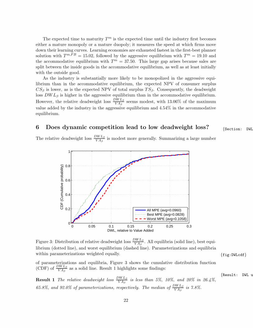
The relative deadweight lossDWLβ

V Aβis modest more generally. Summarizing a large number

0 0.05 0.1 0.15 0.2 0.25 0.30

0.2

0.4

0.6

0.8

1

DWL, relative to Value Added

CD

F (

Cum

ulat

ive

prob

abili

ty)

All MPE (avg=0.0960)Best MPE (avg=0.0828)Worst MPE (avg=0.1058)

Figure 3: Distribution of relative deadweight lossDWLβ

V Aβ. All equilibria (solid line), best equi-

librium (dotted line), and worst equilibrium (dashed line). Parameterizations and equilibriawithin parameterizations weighted equally. fig:DWLcdf

of parameterizations and equilibria, Figure 3 shows the cumulative distribution function(CDF) of

DWLβ

V Aβas a solid line. Result 1 highlights some findings:

Result: DWL under

Result 1 The relative deadweight lossDWLβ

V Aβis less than 5%, 10%, and 20% in 26.4%,

65.8%, and 92.0% of parameterizations, respectively. The median ofDWLβ

V Aβis 7.8%.

22

There is a large relative deadweight lossDWLβ

V Aβin a small number of parameterizations

that occur when the industry almost fails to take off (in the sense that 1− φ1(0, 0)2 ≈ 0.01)

because the outside good is highly attractive. Near this “cusp of viability” the contributionof the inside goods to the expected NPV of total surplus is small and thus V Aβ ≈ 0.

Recall that we average over equilibria at a given parameterization to obtain the dis-tribution of

DWLβ

V Aβ. To look behind these averages, we consider the best equilibrium with

the highest value of TSβ at a given parameterization as well as the worst equilibrium with

the lowest value of TSβ. Figure 3 shows the resulting distributions ofDWLβ

V Aβusing a dot-

ted line for the best equilibrium and a dashed line for the worst equilibrium, and Result 2summarizes: Result: DWL under

Result 2 (1) For the best equilibrium, the relative deadweight lossDWLβ

V Aβis less than 5%,

10%, and 20% in 44.2%, 71.1%, and 92.1% of parameterizations, respectively. The medianof

DWLβ

V Aβis 5.7%. (2) For the worst equilibrium, the relative deadweight loss

DWLβ

V Aβis less

than 5%, 10%, and 20% in 18.7%, 56.4%, and 91.8% of parameterizations, respectively. Themedian of

DWLβ

V Aβis 9.2%.

Hence, even in the worst equilibria the relative deadweight lossDWLβ

V Aβis modest for a wide

range of parameterizations.Closer inspection shows that the best equilibrium is often accommodative in nature

whereas the worst equilibrium is often aggressive. In Appendix C we offer formal definitionsof aggressive and accommodative equilibria and show that they are closely linked to theworst, respectively, best equilibria. To facilitate the exposition and build intuition, in whatfollows we therefore identify the best equilibrium with an accommodative equilibrium and theworst equilibrium—to the extent that it differs from the best equilibrium—with an aggressiveequilibrium.24 If the equilibrium is unique, then we identify it with an accommodativeequilibrium.

6.1 Deadweight loss in perspective: static non-cooperative pricing coun-

terfactual

Is a relative deadweight lossDWLβ

V Aβof 10% of the maximum value added by the industry

“small” and a relative deadweight loss of 30% “large”? To help put these percentages inperspective, we show that the deadweight loss is lower than expected in view of the twotraditional roles of price (allocative and distributional). To this end, we shut down theinvestment role of price. In the price-setting phase, incumbent firm 1 is thus left to maximizestatic profit:

maxp1

D1(p1, pSN2 (e))(p1 − c(e1)).

Hence, the pricing decision pSN1 (e) in this static non-cooperative pricing counterfactual isuniquely determined by the first-order condition

pSN1 (e) = c(e1) +σ

1−D1(pSN1 (e), pSN2 (e))

.

24This association is not perfect. For some parameterizations (e.g., those with weak product differentiation),there are multiple equilibria all of which are aggressive and none of which are accomodative.

23

The expected NPV of incumbent firm 1 is

V SN1 (e) = D1(p

SN1 (e), pSN2 (e))(pSN1 (e)− c(e1))

+USN1 (e) +

2∑

n=1

Dn(pSN1 (e), pSN2 (e))

[USN1

(en+

)− USN

1 (e)]

and, in contrast to the pricing decision, accounts for the impact of a sale on the valueof continued play. Finally, the exit-entry phase remains unchanged.25 Our computationsalways led to a unique solution.

The fifth column of Table 3 shows our metrics for industry structure, conduct, and perfor-mance for the static non-cooperative pricing counterfactual at the baseline parameterization.Similar to the accommodative equilibrium, the counterfactual involves both over-entry andunder-exit (NSN

1 = 2.00 and NSN∞ = 2.00). Learning economies are exhausted even more

slowly than in the accommodative equilibrium (Tm,SN = 53.91 > 37.45 = Tm) becausefirms ignore the investment role of price in making their pricing decisions. The deadweightloss DWLβ increases more than threefold relative to the accommodative equilibrium and bymore than a quarter relative to the aggressive equilibrium.

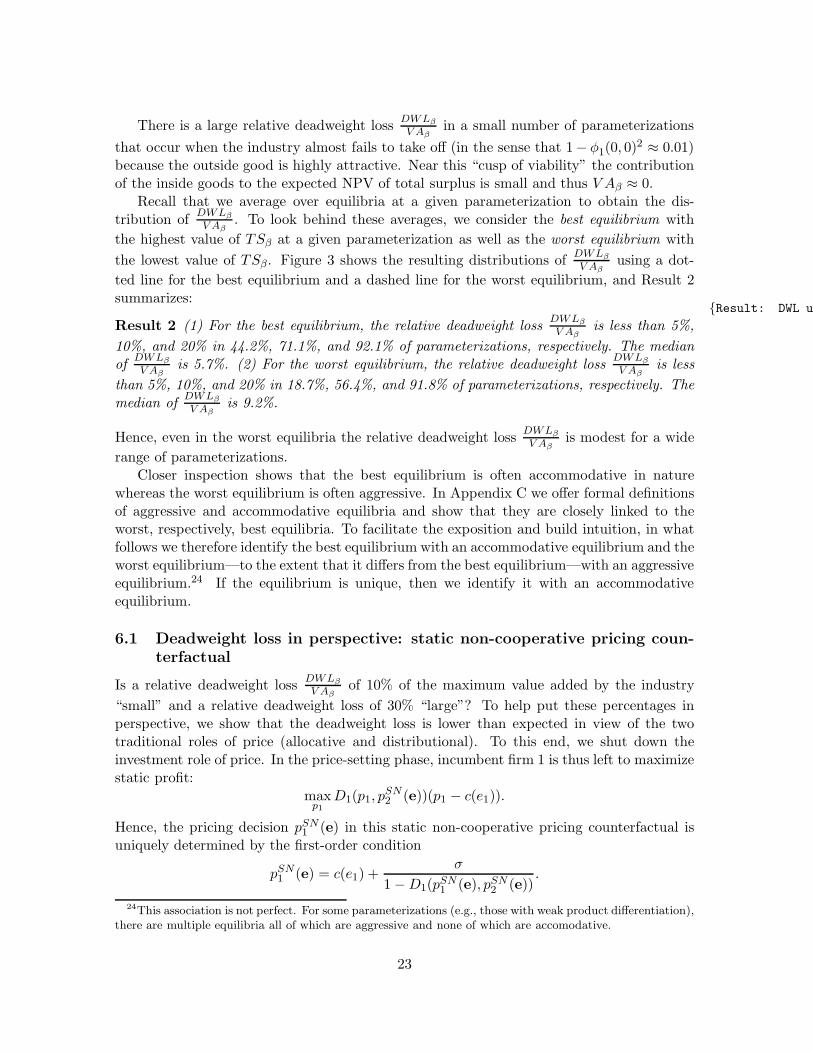
The investment role of price is socially beneficial more generally. Figure 4 shows the

10−2

10−1

100

101

102

0

0.2

0.4

0.6

0.8

1

ratio of DWL(0,0)’s: SN/MPE (ratio>1 implies that SNP is worse)

CD

F (

Cum

ulat

ive

prob

abili

ty)

E(ratio)=4.155Pr(r<1)=0.19, E(r|r<1)=0.487

Figure 4: Distribution of deadweight loss ratioDWLSN

β

DWLβ. Log scale. Parameterizations and

equilibria within parameterizations weighted equally. fig:SNDWLgap

distribution of the deadweight loss ratioDWLSN

β

DWLβ. Note that

DWLSNβ

DWLβis independent of our

normalization by V Aβ. Result 3 summarizes:Result: difference

Result 3 DWLSNβ is at least as large as DWLβ in 81% of cases, at least twice as large in

44% of cases, and at least five times as large in 14% of cases. The median ofDWLSN

β

DWLβis 11.

25Our static non-cooperative pricing counterfactual loosely corresponds to the version of the war of attritionpresented in Tirole (1988), with the addition of learning-by-doing and product differentiation.

24

DWLSNβ is smaller than DWLβ in a number of parameterizations that mostly involve an

unattractive outside good (p0 ≥ 15). Because the outside good constrains pricing decisionsand profitability much more in a monopolistic than in a duopolistic industry, a less attractiveoutside good sharpens the incentive to monopolize the industry in equilibrium. But if firmsignore the investment role of price in the static non-cooperative pricing counterfactual, thena duopolistic industry with a lower deadweight loss emerges.

Generally speaking, we conclude that dynamic competition leads to low deadweight loss.The deadweight loss is low not only relative to the maximum value added by the industry,it is also smaller than the deadweight loss that arises if firms ignore the investment role ofprice.26 Put differently, the investment role of price is by and large socially beneficial. Thestatic non-cooperative pricing counterfactual also shows that a low deadweight loss is almostcertainly not hardwired into the primitives of our learning-by-doing model. Instead, thereis something in the nature of the investment role of price and dynamic competition that inequilibrium leads to low deadweight loss.

6.2 Differences between equilibria and first-best planner solution

Dynamic competition leads to low deadweight loss despite distortions in pricing, exit, andentry. Indeed, as we next show, there are typically substantial differences between theequilibria and the first-best planner solution. Paradoxically, the best equilibrium can differeven more from the planner solution than the worst equilibrium.

Recall that too low prices cause deadweight loss from overproduction, just as too highprices cause deadweight loss from underproduction. To illustrate that the equilibria involveprices that are too low, we first define 1 [p1(e) < c(e1) for some e ∈ 1, . . . ,M × 0, . . . ,M]to indicate that a price is below the marginal cost of production in at least one state. Second,we define 1

[p1(e) < pFB

1 (e) for some e ∈ 1, . . . ,M × 0, . . . ,M]to indicate that a price

is below the first-best planner solution in some state. Figure 5 shows the distribution ofthese indicators and Result 4 summarizes:

Result: MPE prices

Result 4 (1) p1(e) < c(e1) for some e ∈ 1, . . . ,M×0, . . . ,M in all equilibria in 80% ofparameterizations.(2) p1(e) < pFB

1 (e) for some e ∈ 1, . . . ,M×0, . . . ,M in all equilibriain 63% of parameterizations.

We caution that the states with too low prices are not necessarily on the equilibrium pathstarting from state (0, 0).

We next turn from pricing to exit and entry and compare the expected short-run andlong-run number of firms between the equilibria and the first-best planner solution. Figure 6shows the distribution of N1 −NFB

1 as a solid line and Result 5 highlights some findings:

Result: MPE involvesResult 5 N1 is larger than NFB

1 in 78% of parameterizations and smaller than NFB1 in less

than 1% of parameterizations.

26We also find that the deadweight loss under competition is lower than the deadweight loss that ariseswhen firms behave collusively with respect to both pricing and entry/exit decisions. For the baseline pa-rameterization, the deadweight loss as a percentage of value added in the fully collusive solution is 14.32percent.

25

0 0.1 0.2 0.3 0.4 0.5 0.6 0.7 0.8 0.9 10

0.2

0.4

0.6

0.8

1

Share of price below threshold

CD

F (

Cum

ulat

ive

prob

abili

ty)

p<costp<p

FCP

Figure 5: Distribution of 1 [p1(e) < c(e1) for some e ∈ 1, . . . ,M × 0, . . . ,M] and1[p1(e) < pFB

1 (e) for some e ∈ 1, . . . ,M × 0, . . . ,M]. Parameterizations and equilibria

within parameterizations weighted equally. Figure: MPE and

−2 −1.5 −1 −0.5 0 0.5 1 1.5 20

0.2

0.4

0.6

0.8

1

Difference in Number of Firms at T=1, (MPE − FCP)

CD

F (

Cum

ulat

ive

prob

abili

ty)

All MPE (avg=0.5576)Best MPE (avg=0.5588)Worst MPE (avg=0.5576)

Figure 6: Distribution of N1 − NFB1 . All equilibria (solid line), best equilibrium (dotted

line), and worst equilibrium (dashed line). Parameterizations and equilibria within param-eterizations weighted equally. Figure: distribution

26

Thus, the equilibria typically have too many firms in the short run, consistent with over-entry. They very rarely have too few firms in the short run. Figure 6 also breaks out thebest equilibrium as a dotted line and the worst equilibrium as a dashed line. Similar to ourexamples in Section 5.2, there is no discernible difference between the best and the worstequilibrium.

Figure 7 shows the distribution of N∞ − NFB∞ as a solid line and breaks out the best

equilibrium as a dotted line and the worst equilibrium as a dashed line. Result 6 summarizes:

−2 −1.5 −1 −0.5 0 0.5 1 1.5 20

0.2

0.4

0.6

0.8

1

Difference in Number of Firms at T=∞, (MPE − FCP)

CD

F (

Cum

ulat

ive

prob

abili

ty)

All MPE (avg=0.1901)Best MPE (avg=0.3580)Worst MPE (avg=0.1631)

Figure 7: Distribution N∞−NFB∞ . All equilibria (solid line), best equilibrium (dotted line),

and worst equilibrium (dashed line). Parameterizations and equilibria within parameteriza-tions weighted equally. Figure: CDF of

Result: MPE involves

Result 6 (1) N∞ is larger than NFB∞ in 60% of parameterizations and smaller than NFB

∞

in 5% of parameterizations. (2) For the best equilibrium, N∞ is larger than NFB∞ in 62%

of parameterizations and smaller than NFB∞ in 1% of parameterizations. (3) For the worst

equilibrium, N∞ is larger than NFB∞ in 62% of parameterizations and smaller than NFB

∞ in7% of parameterizations.

Thus, the equilibria regularly have too many firms in the long run, consistent with under-exit. This tendency is exacerbated in the best equilibrium. The equilibria very rarely havetoo few firms in the long run.

We finally turn to the speed at which firms move down their learning curves. Recallthat the expected time to maturity Tm depends on both the number of incumbent firms andtheir pricing decisions. Figure 8 shows the distribution of Tm − Tm,FB as a solid line andbreaks out the best equilibrium as a dotted line and the worst equilibrium as a dashed line.Result 7 summarizes:

Result:TM

27

−100 −80 −60 −40 −20 0 20 40 60 80 1000

0.2

0.4

0.6

0.8

1

Difference in mean Time to Floor (MPE − FCP)

CD

F (

Cum

ulat

ive

prob

abili

ty)

All MPE (avg=11.1485)Best MPE (avg=14.4592)Worst MPE (avg=10.9735)

Figure 8: Distribution of Tm − Tm,FB. All equilibria (solid line), best equilibrium (dottedline), and worst equilibrium (dashed line). Parameterizations and equilibria within param-eterizations weighted equally. fig:TM

Result 7 (1) Tm is larger than Tm,FB in 91% of parameterizations and smaller than Tm,FB

in 8% of parameterizations. (2) For the best equilibrium, Tm is larger than Tm,FB in 94%of parameterizations and smaller than Tm,FB in 7% of parameterization. (3) For the worstequilibrium, Tm is larger than Tm,FB in 91% of parameterizations and smaller than Tm,FB

in 8% of parameterizations.

The speed of learning in the equilibria is generally too slow. Moreover, the best equilibriumexhausts learning economies even more slowly than the worst equilibrium. This is becausepricing is initially less aggressive and more firms split sales in an accommodative equilibriumthan in an aggressive equilibrium.

7 Why does dynamic competition lead to low deadweight

loss? Section: Decomposition

Section 6 leaves us with a puzzle. Dynamic competition leads to low deadweight loss, but thisis not because the equilibrium resembles the first-best planner solution. On the contrary, thebest equilibrium can differ even more from the planner’s solution than the worst equilibrium.

7.1 Decomposition

To better understand why dynamic competition leads to low deadweight loss, we quantifythe importance of three factors that together make up deadweight loss: pricing conduct, exitand entry conduct, and market structure. We accordingly decompose the deadweight loss

28

in equation (12) as

DWLβ = TSFBβ − TSβ = DWLPR

β +DWLEEβ +DWLMS

β ,

where

DWLPRβ =

∞∑

t=0

βt∑

e

µt(e)[CSFB(e) + ΠFB(e)− (CS(e) + Π(e))

], (17) eq:T1

DWLEEβ =

∞∑

t=0

βt∑

e

µt(e)[PSFB(e)−ΠFB(e)− (PS(e)−Π(e))

], (18) eq:T2

DWLMSβ =

∞∑

t=0

βt∑

e

[µFBt (e)− µt (e)

]TSFB(e), (19) eq:T3

and, recall, Π(e) =∑2

n=1Dn(p(e))(pn(e)− c(en)). ΠFB(e) is defined analogously.

The pricing distortion DWLPRβ in equation (17) is the incremental deadweight loss due

to state-wise differences in pricing conduct between the equilibrium and the first-best plannersolution.27

PS(e)−Π(e) is the difference of producer surplus and the static profit of the incumbentfirms in state e and thus the part of producer surplus that accounts for scrap values and setupcosts. The exit and entry distortion DWLEE

β in equation (18) is therefore the incrementaldeadweight loss due state-wise differences in exit and entry conduct between the equilibriumand the first-best planner solution. Expected inflows from scrap values in state e contributepositively to PS(e) − Π(e) and expected outflows from setup costs negatively. A positivevalue ofDWLEE

β thus reflects a tendency for over-entry or under-exit relative to the first-bestplanner solution while a negative value reflects a tendency for under-entry or over-exit.

The market structure distortion DWLMSβ in equation (19) is the incremental deadweight

loss due to differences in the evolution of the industry over time between the equilibriumand the first-best planner solution. Recall that the state e completely describes the num-ber of incumbent firms—and therefore the extent of product variety—along with their costpositions. A negative value of DWLMS

β therefore indicates that the equilibrium puts more

weight on more favorable market structures with higher values of TSFB(e) than the plannersolution; a positive value indicates the reverse. Note that TSFB(e) is high if firms’ costpositions in state e in relation to the price of the outside good yield large gains from trade.

27In our model, there is no distinction between price and quantity distortions. Indeed, consumer surpluscan be written as a function of quantities rather than prices as

CS(Q) = v − σ

2∑

n=0

lnQn −2∑

n=0

Pn(Q)Qn,

where Q ≡ (Q0, Q1, Q2) and (P0(Q), P1(Q), P2(Q)) solve

P0(Q) = p0

Q1 = D1 (p0, P1(Q), P2(Q))

Q2 = D2 (p0, P1(Q), P2(Q)) .

29

TSFB(e) is also high if a large number of firms fosters product variety. Perhaps less obvi-ously, TSFB(e) is high if in state e there are too many firms from the perspective of thefirst-best planner, thus allowing the planner to receive scrap values by ceasing to operateexcess firms. Of course, these last two effects of the number of firms are mutually exclu-sive. The factors contributing to a negative value of DWLMS

β are therefore over-entry andunder-exit as well as fast exploitation of learning economies. Factors contributing to a pos-itive value of DWLMS

β are under-entry, over-exit, slow exploitation of learning economies,and cost inefficient exit. This last phenomenon—which we saw could arise in the two-stepversion of our model—contributes to a positive value of DWLMS

β in the same way that slowexploitation of learning economies does: it makes it more likely that the industry stays inhigher cost states than it would have under the planner’s solution. Table 4 summarizes thedistortions that the signs of DWLEE

β and DWLMSβ indicate.

term positive negative

DWLEEβ Over-entry, under-exit Under-entry, over-exit

DWLMSβ Under-entry, over-exit, slow ex-

ploitation of learning economies,cost inefficient exit

Over-entry, under-exit, fast ex-ploitation of learning economies

Table 4: Decomposition terms and contributing distortions. Table: summary

DWLEEβ and DWLMS

β can offset each other as they depend on over-entry and under-exit

in opposite ways. We therefore define the non-pricing distortion as DWLNPRβ = DWLEE

β +

DWLMSβ . It reflects (1) the net social loss from a suboptimal number of firms (setup costs

net of scrap values net of social benefits of product variety) and (2) the gross social lossfrom a suboptimal exploitation of learning economies and (3) the gross social loss fromcost-inefficient exit.

Examples. Table 5 illustrates the decomposition for the aggressive and accommodativeequilibria at the baseline parameterization. The pricing distortion DWLPR

β = 10.78 is the

DWLβ DWLPRβ DWLEE

β DWLMSβ DWLNPR

β

aggr. eqbm. 14.43 10.78 4.67 -1.01 3.66accom. eqbm. 5.01 2.35 7.32 -4.67 2.66

Table 5: Decomposition. Aggressive and accommodative equilibrium. Baseline parameteri-zation. tbl:DecompBasel

largest part of deadweight loss DWLβ = 14.43 in the aggressive equilibrium. It is mainlydriven by the high expected long-run average price p∞ = 8.28 (see Table 3) that results as theindustry most likely evolves into an mature monopoly. In the accommodative equilibrium,the pricing distortion DWLPR

β = 2.35 is a smaller part of deadweight loss DWLβ = 5.01

because the industry evolves into a mature duopoly. Interestingly, DWLPRβ is small even

though the expected long-run average price p∞ = 5.24 is almost two-thirds larger than in

30

the first-best planner solution (pFB∞ = 3.25).28

In the accommodative equilibrium, the largest part of deadweight loss DWLβ = 5.01is the exit and entry distortion DWLEE

β = 7.32. This reflects both wasteful duplicationof setup costs due to over-entry and scrap values that firms forgo in equilibrium due tounder-exit. The latter is analogous to the wasteful duplication of per-period, avoidable fixedcosts that arises in the standard war of attrition model in Tirole (1988).29 In contrast, inthe aggressive equilibrium DWLEE

β = 4.67 is a smaller part of DWLβ = 14.43 because thefollower is likely to eventually exit the industry and receive the scrap value.

In both equilibria, the market structure distortion DWLMSβ is negative, indicating that

the industry spends more time in favorable market structures than in the first-best plannersolution. This is driven by over-entry and under-exit as opposed to fast exploitation oflearning economies. Indeed, in both equilibria learning economies are exhausted more slowly(Tm = 19.10 and Tm = 37.50, see again Table 3) than in the planner solution (Tm,FB =15.02).

As DWLMSβ partially offsets DWLEE

β , the non-pricing distortion DWLNPRβ = 3.66 is

much smaller than the pricing distortion DWLPRβ = 10.78 in the aggressive equilibrium.

In the accommodative equilibrium the non-pricing distortion DWLNPRβ = 2.66 is slightly

larger than the pricing distortion DWLPRβ = 2.35.

General results. Figure 9 shows the distribution ofDWLPR

β

DWLβ,

DWLEEβ

DWLβ,

DWLMSβ

DWLβ, and

DWLNPRβ

DWLβ. We scale each term of the decomposition by DWLβ to better gauge its size.

Result 8 highlights some findings:Result: Sign of

Result 8 (1) The pricing distortion DWLPRβ is positive in 98% of parameterizations. (2) The

exit and entry distortion DWLEEβ is positive in 81% of parameterizations. (3) The market

structure distortion DWLMSβ is negative in 70% of parameterizations. (4) The non-pricing

distortion DWLNPRβ is positive in 92% of parameterizations.

DWLEEβ is typically positive by part (2) of Result 8 because of over-entry and under-exit.

Also because of over-entry and under-exit, DWLMSβ is typically negative by part (3), as the

speed of learning in the equilibria is generally too slow (see Figure 8 and Result 7). Thus, ashighlighted in Result 9, DWLMS

β typically offsets DWLEEβ so that DWLNPR

β is very oftensmaller than its largest component (in absolute value):

Result: Offset

Result 9 |DWLNPRβ | is less than max

∣∣∣DWLEEβ

∣∣∣ ,∣∣∣DWLMS

β

∣∣∣

in 88% of parameteriza-

tions.

Parts (1) and (4) of Result 8 show that generally both pricing and non-pricing distortionscontribute to deadweight loss. As Result 10 shows, the pricing distortion is often larger thanthe non-pricing distortion:

28Dynamic first-best prices(pFB1 (e), pFB

2 (e)), in turn, coincide with static first-best prices (c(e1), c(e2)) if

e1 ≥ m and e2 ≥ m.29In the Online Appendix, we will establish that our model with scrap values is formally equivalent to a

model with per-period, avoidable fixed costs but without scrap values.

31

−2 −1.5 −1 −0.5 0 0.5 1 1.5 20

0.2

0.4

0.6

0.8

1

DWL terms, relative to DWL

CD

F (

Cum

ulat

ive

prob

abili

ty)

PR: pricing (avg= 0.733)EE: exit & entry (avg= 1.644)MS: structure (avg=−1.377)EE+MS: non−price (avg= 0.267)

Figure 9: Distribution ofDWLPR

β

DWLβ,

DWLEEβ

DWLβ,

DWLMSβ

DWLβ, and

DWLNPRβ

DWLβ. Parameterizations and

equilibria within parameterizations weighted equally. fig:DecompMPE

Result: PR distortionResult 10 The pricing distortion DWLPR

β is larger than the non-pricing distortion DWLNPRβ

in 73% of parameterizations.

7.2 Why is the best equilibrium so good?

The deadweight loss in the best equilibrium is small although it often differs greatly fromthe first-best planner solution. Recall that the best equilibrium is often accommodative.

To see why the deadweight loss in an accommodative equilibrium is small, we show ina first step that the pricing distortion DWLPR

β is small. Recall from Result 10 that thepricing distortion is often larger than the non-pricing distortion. In a second step, we arguethat the non-pricing distortion DWLNPR

β is small because of the social benefit of productvariety.

Why is the pricing distortion small? At first blush, there appears to be no reasonfor the pricing distortion in an accommodative equilibrium to be particularly small. Atthe baseline parameterization, equilibrium prices (p1(e), p2(e)) substantially exceed staticfirst-best prices (c(e1), c(e2)) even once the industry becomes a mature duopoly.

Proposition 2, however, bounds the contribution CSFB(e) + ΠFB(e) − (CS(e) + Π(e))to the pricing distortion DWLPR

β by the demand for the outside good D0(p(e)):

Proposition: TaylorProposition 2 Consider a symmetric state e = (e, e), where e > 0. If p0 ≥ κ, p1(e) > c(e),and D0(p(e)) <

12 , then

CSFB(e) + ΠFB(e)− (CS(e) + Π(e)) ≤ (p1(e)− c(e))2

σD0(p(e))(1 −D0(p(e))). (20) eq: Taylor approx

32

Note that the bound on the right-hand side of equation (20) approaches zero as the demandfor the outside good approaches zero. This often has bite: as the incumbent firms movedown their learning curves, they improve their cost positions relative to the price of theoutside good and drive the share of the outside good close to zero. Exceptions occur only iflearning economies are weak—ρ is close to 1—or inconsequential because the outside goodis highly attractive.

While the bound on the right-hand side of equation (20) relies on logit demand, theintuition is more general. To a first-order approximation, the deadweight loss due to marketpower decreases as market demand becomes less price elastic (Harberger 1954). With logitdemand, a decrease in the price elasticity of the aggregate demand D1 +D2 for the insidegoods is associated with a decreased share D0 of the outside good. In the Online Appendix,we will show that a similar property holds for linear demand with differentiated products.

Why is the non-pricing distortion small? Recall that the non-pricing distortionDWLNPRβ =

DWLEEβ +DWLMS

β reflects the net social loss from a suboptimal number of firms as wellas the gross social losses from suboptimal exploitation of learning economies and cost ineffi-cient exit. Recall, too, that, broadly speaking, in particular accommodative equilibria havetoo many firms, both in the short run and in the long run, consistent with over-entry andunder-exit (Results 5, 6, and parts (2) and (3) of 8). Negative values of DWLMS

β thus tend

to offset positive values of DWLEEβ (Result 9).

Of course, too many firms give rise to a social loss from the wasteful duplication of setupcosts due to over-entry and scrap values that firms forgo in equilibrium due to under-exit.However, there is a “silver lining”: too many firms give rise to a social benefit from additionalproduct variety. Because of the social benefit of product variety, the net social loss fromtoo many firms is small. This is especially relevant because accommodative equilibria tendto arise when the degree of product differentiation σ is high. Hence, the social benefit ofproduct variety tends to be large.

Learning economies accentuate the silver lining of additional product variety. Supposethe industry evolves into a mature duopoly in an accommodative equilibrium and into amature monopoly in the first-best planner solution, and that there is no further exit andentry. Then there exists a period t∗ such that for period t ≥ t∗, the equilibrium transientdistribution µt (e) puts all mass on state e, where e1 ≥ m and e2 ≥ m, and the first-best transient distribution µFB

t (e) puts all mass on state e, where either e1 ≥ m ande2 = 0 or e1 = 0 and e2 ≥ m. Because learning economies are exhausted and there isno further exit and entry, we have TSFB(e) = TSFB(m,m) if e1 ≥ m and e2 ≥ m, andTSFB(e) = TSFB(m, 0) if either e1 ≥ m and e2 = 0 or e1 = 0 and e2 ≥ m. Moreover,TSFB(m,m) = CSFB(m,m) and TSFB(m, 0) = CSFB(m, 0) because the planner sets staticfirst-best prices. Hence, the market structure distortion DWLMS

β can be approximated as

t∗∑

t=0

βt∑

e

[µFBt (e)− µt (e)

]TSFB(e)− βt∗+1

1− β

[CSFB(m,m)− CSFB(m, 0)

],

where the last term can be thought of as a reduction in DWLMSβ —and thus in the non-

pricing distortion DWLNPRβ —due to the social benefit of additional product variety. From

33

equation (10) it is straightforward to establish that

CSFB(m,m)− CSFB(m, 0)

= σ

(ln

(exp

(−p0σ

)+ 2exp

(−c(m)

σ

))− ln

(exp

(−p0σ

)+ exp

(−c(m)

σ

))),

where c(m) = κρlog2 m from equation (1), and

d(CSFB(m,m)− CSFB(m, 0))

dρ= − (2D1(c(m), c(m)) −D1(c(m),∞)) κρlog2 m−1 log2m < 0,

since 2D1(c(m), c(m)) = 2

2+exp(−(

p0−c(m)σ

)) > 1

1+exp(−(

p0−c(m)σ

)) = D1(c(m),∞). Hence, as

learning economies strengthen, the reduction in DWLMSβ and DWLNPR

β due to the socialbenefit of additional product variety increases.

7.3 Why is the worst equilibrium not so bad?

Recall that the worst equilibrium is aggressive. To see why the deadweight loss in anaggressive equilibrium is small (albeit not as small as in the best equilibrium), we showin a first step that the pricing distortion DWLPR

β is small. In a second step, we argue that

the non-pricing distortion DWLNPRβ is small because of a fairly efficient winnowing out of

firms.We emphasize that the arguments below do not imply that the deadweight loss in an

aggressive equilibrium is close to zero. Rather, each one speaks to an economic force in themodel that serves as a “headwind” that keeps the deadweight loss from becoming excessivelylarge.

Why is the pricing distortion small? There again appears to be no reason for thepricing distortion in an aggressive equilibrium to be small. At the baseline parameteriza-tion, the industry evolves into a mature monopoly. Proposition 2 bounds the contributionCSFB(e) + ΠFB(e) − (CS(e) + Π(e)) to the pricing distortion DWLPR

β by the degree of

product differentiation σ and the advantage-building motive U1

(e1+)− U1 (e):

Proposition: MonopolyProposition 3 Consider a state e = (e, 0), where e > 0. Then

CSFB(e) + ΠFB(e)− (CS(e) + Π(e))

<

σ if 0 ≤ U1

(e1+)− U1 (e) < σ

(1 + exp

(p0−c(e)

σ

)),

σ +∣∣U1

(e1+)− U1 (e)

∣∣ otherwise.

(21) eq: Monopoly DWL

Note that the bound on the right-hand side of equation (21) approaches σ as the incumbentfirm moves down its learning curve and U1

(e1+)− U1 (e) approaches zero. While Propo-

sition 3 relies on logit demand, the intuition that the threat of substitution to the outsidegood holds market power in check transcends the logit specification.

34

Proposition 3 has bite because aggressive equilibria tend to arise when the degree ofproduct differentiation σ is low. This is intuitive: pricing aggressively to marginalize one’srival or altogether force it from the industry is especially attractive if products are closesubstitutes so that firms on an equal footing would fiercely compete.

Why is the non-pricing distortion small? While an aggressive equilibrium usuallyinvolves delayed exit (relative to the first-best planner solution), it involves rather briskeventual exit. Thus, the industry usually quickly evolves towards the first-best marketstructure in an aggressive equilibrium, which tends to keep DWLMS

β , and thus DWLNPRβ ,

small. The small non-pricing distortion reflects the resulting relatively low net social lossfrom a suboptimal number of firms. Put another way, in an aggressive equilibrium, this netsocial loss is small because competition for the market resolves itself quickly and winnowsout firms in a fairly efficient way.

8 Conclusion Section: Conclusions

This paper studies a setting in which the traditional allocative and distributive roles ofpricing are supplemented by a third role: investment. The investment role, which ariseswhen firms jostle for competitive advantage through the prices they set, leads to dynamiccompetition.

In the introduction we floated the idea that it should be obvious that dynamic competi-tion along a learning curve would be extremely efficient. In contrast to dynamic competitionin rent-seeking models or even conventional wars of attrition where competition among firmssquanders resources, competition in our setting creates socially valuable know-how as firmsmove down their learning curves. And instead of throwing this surplus away on wastefulactivities, firms transfer it to consumers through lower prices.

However, our computations illustrate that the conduct and market structure that ariseunder dynamic competition often differ greatly from the conduct and structure that a first-best planner prefers: dynamic competition usually does not look like the socially efficientsolution. Moreover, as the special case of our model with a two-step learning curve illus-trates, even if price competition transfers all the benefits of learning economies from firms toconsumers, the presence of a learning curve does not eliminate wasteful coordination failuresthat can arise in natural monopoly markets. In sum, dynamic competition when pricing hasan investment role is not a “magic bullet” that completely eliminates inefficiencies that canarise in dynamic or static interactions in oligopoly markets.

Still, our results suggest the following conclusion: when price has an investment roledynamic competition operates reasonably efficiently. Learning economies in our model re-duce competition from the outside good so much that it minimizes quantity distortions fromoligopoly pricing. The presence of learning economies in our model also tends to bias theentry process toward generating more entry rather than less, making it more likely that thereis eventually competition in the market. Of course, excessive entry into a market which aplanner would monopolize is inefficient because it gives rise to a duplication of setup costs.But when there is sufficiently strong product differentiation, we tend to get accommodativeequilibria in which two firms persist in the industry, creating long-run gains from product

35

variety that partially offset this inefficiency. And when product differentiation is weak, ag-gressive equilibria arise which, although they usually involve delayed exit (relative to thefirst-best planner solution), involve fairly quick eventual exit, evolving the industry rapidlyto the first-best market structure.

So why is dynamic competition reasonably efficient in our model? Ultimately, the answerboils down to the key fundamental that creates the investment role of price in the first place:the learning curve.

• The learning curve is a powerful force for minimizing pricing distortions in accom-modative equilibria evolving into a mature duopoly in the long run.

• The learning curve helps lead to an outcome in which exit and entry distortions erron the side of too many firms than too few firms, and the distortions are partly offsetby benefits from product variety (in accommodative equilibria) or eventual exit (inaggressive equilibria).

• Learning economies accentuate the long-run benefits from product variety when thereis over-entry and under-exit in accommodative equilibria.

Put simply, when price serves as an investment, dynamic competition is efficient because ofthe efficiency-enhancing properties of the investment.

From a policy perspective, our results suggest that in settings in which price serves as aninvestment, the upside from competition policy or regulatory interventions—beyond thoseaimed at preventing firms from colluding on price and entry/exit decisions—is likely to befairly limited.30 Though we show in Besanko et al. (2014) that welfare gains from conductrestrictions on pricing are possible in the setting we analyze here, achieving those gains wouldrequire detailed knowledge of demand and cost parameters. Unless a competition authorityexecutes flawlessly based on exact knowledge of market primitives, it may be better not tointervene (except to police collusive behavior) and tolerate the “not so bad” welfare lossesthat would typically arise under dynamic competition.

30Analysis (not shown in the paper) suggests that enforcement of statutes against collusion is likely to beimportant in our setting. Not only does full collusion lead to higher deadweight losses than dynamic compe-tition does, it results in significantly lower consumer surplus. For example, in the baseline parameterization,the discounted present value of consumer surplus under the fully collusive solution is 32.54, as compared to93.87 and 103.29 under the aggressive and acommodative equilibrium, respectively. (The latter two numberscome from Table 3

36

A Omitted expressions Section: Appendix2

Exit decision of incumbent firm. The probability of incumbent firm 1 exiting the ap:ExitExpressindustry in state e′ is

φ1(e′) = 1− FX(X1(e

′))

=

1 if X1(e′) < X −∆X ,

12 −

[X1(e′)−X]2∆X

if X1(e′) ∈ [X −∆X ,X +∆X ],

0 if X1(e′) > X +∆X

and the expectation of the scrap value conditional on exiting the industry is

EX

[X1|X1 ≥ X1(e

′)]

=

∫ X+∆X

F−1X

(1−φ1(e′))X1dFX(X1)

φ1(e′)

=1

φ1(e′)

[ZX (0)− ZX

(1− φ1(e

′))],

where

ZX (1− φ) =1

∆2X

−16

(X −∆X

)3if 1− φ ≤ 0,

12

(∆X −X

) (F−1X (1− φ)

)2+ 1

3

(F−1X (1− φ)

)3if 1− φ ∈

[0, 12],

12

(∆X +X

) (F−1X (1− φ)

)2 − 13

(F−1X (1− φ)

)3 − 13X

3if 1− φ ∈

[12 , 1],

16

(X +∆X

)3 − 13X

3if 1− φ ≥ 1

and

F−1X (1− φ) = X +∆X

−1 if 1− φ ≤ 0,

−1 +√

2 (1− φ) if 1− φ ∈[0, 12],

1−√2φ if 1− φ ∈

[12 , 1],

1 if 1− φ ≥ 1.

Entry decision of potential entrant. The probability of potential entrant 1 not entering ap:EntryExpresthe industry in state e′ is

φ1(e′) = 1− FS(S1(e

′))

=

1 if S1(e′) < S −∆S,

12 −

[S1(e′)−S]2∆S

if S1(e′) ∈ [S −∆S , S +∆S ],

0 if S1(e′) > S +∆S

and the expectation of the setup cost conditional on entering the industry is

ES

[S1|S1 ≤ S1(e

′)]

=

∫ F−1S

(1−φ1(e′))

S−∆SS1dFS(S1)

(1− φ1(e′))

=1

φ1(e′)

[ZS

(1− φ1(e

′))− ZS (1)

],

37

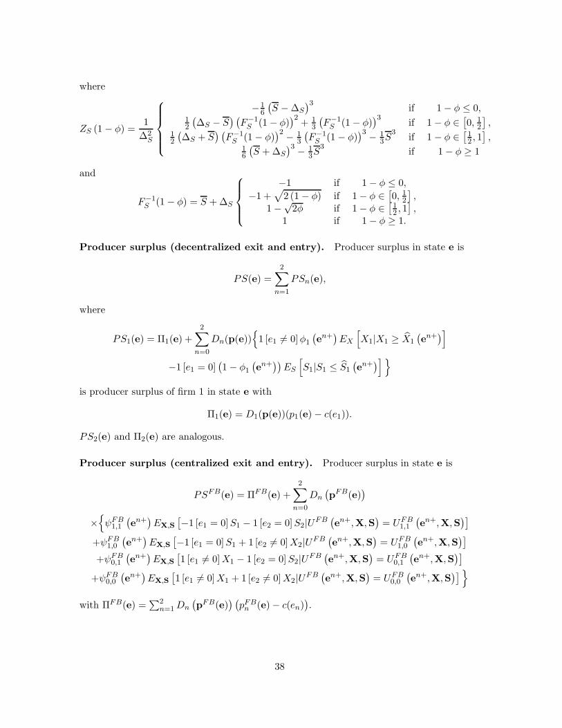
where

ZS (1− φ) =1

∆2S

−16

(S −∆S

)3if 1− φ ≤ 0,

12

(∆S − S

) (F−1S (1− φ)

)2+ 1

3

(F−1S (1− φ)

)3if 1− φ ∈

[0, 12],

12

(∆S + S

) (F−1S (1− φ)

)2 − 13

(F−1S (1− φ)

)3 − 13S

3if 1− φ ∈

[12 , 1],

16

(S +∆S

)3 − 13S

3if 1− φ ≥ 1

and

F−1S (1− φ) = S +∆S

−1 if 1− φ ≤ 0,

−1 +√

2 (1− φ) if 1− φ ∈[0, 12],

1−√2φ if 1− φ ∈

[12 , 1],

1 if 1− φ ≥ 1.

Producer surplus (decentralized exit and entry). Producer surplus in state e is

PS(e) =

2∑

n=1

PSn(e),

where

PS1(e) = Π1(e) +

2∑

n=0

Dn(p(e))1 [e1 6= 0]φ1

(en+

)EX

[X1|X1 ≥ X1

(en+

)]

−1 [e1 = 0](1− φ1

(en+

))ES

[S1|S1 ≤ S1

(en+

)]

is producer surplus of firm 1 in state e with

Π1(e) = D1(p(e))(p1(e)− c(e1)).

PS2(e) and Π2(e) are analogous.

Producer surplus (centralized exit and entry). Producer surplus in state e is

PSFB(e) = ΠFB(e) +

2∑

n=0

Dn

(pFB(e)

)

×ψFB1,1

(en+

)EX,S

[−1 [e1 = 0]S1 − 1 [e2 = 0]S2|UFB

(en+,X,S

)= UFB

1,1

(en+,X,S

)]

+ψFB1,0

(en+

)EX,S

[−1 [e1 = 0]S1 + 1 [e2 6= 0]X2|UFB

(en+,X,S

)= UFB

1,0

(en+,X,S

)]

+ψFB0,1

(en+

)EX,S

[1 [e1 6= 0]X1 − 1 [e2 = 0]S2|UFB

(en+,X,S

)= UFB

0,1

(en+,X,S

)]

+ψFB0,0

(en+

)EX,S

[1 [e1 6= 0]X1 + 1 [e2 6= 0]X2|UFB

(en+,X,S

)= UFB

0,0

(en+,X,S

)]

with ΠFB(e) =∑2

n=1Dn

(pFB(e)

) (pFBn (e)− c(en)

).

38

Industry structure, conduct, and performance. The expected short-run and long-runnumber of firms is

N1 =∑

e

µ1 (e)N(e), N∞ =∑

e

µ∞ (e)N(e),

where number of firms in state e is

N(e) =

2∑

n=1

1 [en > 0] .

The expected long-run average price is

p∞ =∑

e≥(0,0)

µ∞ (e)

1− µ∞(0, 0)p(e),

where (share-weighted) average price in state e is

p(e) =2∑

n=1

Dn(p1(e), p2(e))

1−D0(p1(e), p2(e))pn(e).

The expected time to maturity is

Tm = E [min t ≥ 0|et ∈ Ω| e0 = (0, 0)] ,

where et is the state of the industry in period t and

Ω = (m, 0), . . . , (M, 0), (0,m), . . . , (0,M), (m,m), . . . , (M,M)

is the set of states in which the industry is either a mature monopoly or a mature duopoly.min t ≥ 0|et ∈ Ω is the so-called first passage time into the set of states Ω. It can be shownthat Tm is the solution to a system of linear equations (Kulkarni 1995, equation (4.72)).

The expected NPV of consumer surplus CSβ is defined analogously to the expected NPVof total surplus TSβ in equation (11).

B Proofs Section: Appendix

Proof of Proposition 1. The method of proof is to show, first, that the value functionsand the policy functions in Table 1 are consistent with each other in every state and them toshow that in every state, firms would not make a one-shot deviation from their equilibriumstrategies. The details of this analysis will be presented in the Online Appendix.Proof of Proposition 2. Define the sum of consumer surplus and static profit to be

Φ(p) = CS(p, p) + 2D1(p, p)(p − c(e)).

Using this definition, in a symmetric state e = (e, e), where e > 0, we can write

CSFB(e) + ΠFB(e)− (CS(e) + Π(e)) = Φ(pFB1 (e))− Φ(p1(e)).

39

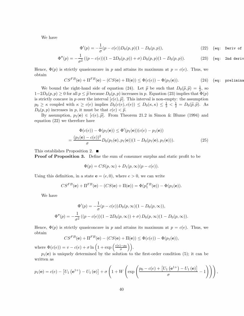
We have

Φ′(p) = − 1

σ(p− c(e))D0(p, p)(1 −D0(p, p)), (22) eq: Deriv of NB(p)

Φ′′(p) = − 1

σ2((p− c(e))(1 − 2D0(p, p)) + σ)D0(p, p)(1 −D0(p, p)). (23) eq: 2nd derive

Hence, Φ(p) is strictly quasiconcave in p and attains its maximum at p = c(e). Thus, weobtain

CSFB(e) + ΠFB(e)− (CS(e) + Π(e)) ≤ Φ(c(e)) − Φ(p1(e)). (24) eq: preliminary

We bound the right-hand side of equation (24). Let p be such that D0(p, p) = 12 , so

1−2D0(p, p) ≥ 0 for all p ≤ p becauseD0(p, p) increases in p. Equation (23) implies that Φ(p)is strictly concave in p over the interval [c(e), p]. This interval is non-empty: the assumptionp0 ≥ κ coupled with κ ≥ c(e) implies D0(c(e), c(e)) ≤ D0(κ, κ) ≤ 1

3 <12 = D0(p, p). As

D0(p, p) increases in p, it must be that c(e) < p.By assumption, p1(e) ∈ [c(e), p]. From Theorem 21.2 in Simon & Blume (1994) and

equation (22) we therefore have

Φ(c(e)) − Φ(p1(e)) ≤ Φ′(p1(e))(c(e) − p1(e))

=(p1(e)− c(e))2

σD0(p1(e), p1(e))(1 −D0(p1(e), p1(e))). (25)

This establishes Proposition 2.Proof of Proposition 3. Define the sum of consumer surplus and static profit to be

Φ(p) = CS(p,∞) +D1(p,∞)(p − c(e)).

Using this definition, in a state e = (e, 0), where e > 0, we can write

CSFB(e) + ΠFB(e)− (CS(e) + Π(e)) = Φ(pFB1 (e))− Φ(p1(e)).

We have

Φ′(p) = − 1

σ(p− c(e))D0(p,∞)(1 −D0(p,∞)),

Φ′′(p) = − 1

σ2((p− c(e))(1 − 2D0(p,∞)) + σ)D0(p,∞)(1−D0(p,∞)).

Hence, Φ(p) is strictly quasiconcave in p and attains its maximum at p = c(e). Thus, weobtain

CSFB(e) + ΠFB(e)− (CS(e) + Π(e)) ≤ Φ(c(e)) − Φ(p1(e)),

where Φ(c(e)) = v − c(e) + σ ln(1 + exp

(c(e)−p0

σ

)).

p1(e) is uniquely determined by the solution to the first-order condition (5); it can bewritten as

p1(e) = c(e) −[U1

(e1+)− U1 (e)

]+ σ

(1 +W

(exp

(p0 − c(e) +

[U1

(e1+)− U1 (e)

]

σ− 1

))),

40

where W (·) is the Lambert W function. Defining x = p0−c(e)σ and y =

U1(e1+)−U1(e)

σ , thiscan be further written as

p1(e) = c(e) + σ (−y + 1 +W (exp(x+ y − 1))) .

Hence,

Φ(p1(e)) = v − c(e) + σ

(ln

(1 +W (exp(x+ y − 1))

W (exp(x+ y − 1))

)+

y

1 +W (exp(x+ y − 1))− 1

)

and

Φ(c(e)) = v − c(e) + σ ln (1 + exp(−x)) .

It follows that

Φ(c(e)) − Φ(p1(e))

= σ

(ln (1 + exp(−x))− ln

(1 +W (exp(x+ y − 1))

W (exp(x+ y − 1))

)− y

1 +W (exp(x+ y − 1))+ 1

)

(26) form1

= σ

(ln (1 + exp(x))− ln (1 +W (exp(x+ y − 1)))−W (exp(x+ y − 1)) +

yW (exp(x+ y − 1))

1 +W (exp(x+ y − 1))

).

(27) form2

Some properties of the Lambert W function are that W (z) is increasing in z, W (0) = 0,and W (z exp(z)) = z for all z ≥ 0.

Case 1: y < 1 + exp(x). We first show that if y < 1 + exp(x), then

ln (1 + exp(−x))− ln

(1 +W (exp(x+ y − 1))

W (exp(x+ y − 1))

)+ 1 < 1. (28) cond2

To see this, note that equation (28) is equivalent to

ln (1 + exp(−x)) ≤ ln

(1 +W (exp(x+ y − 1))

W (exp(x+ y − 1))

)

⇔ exp(−x) < 1

W (exp(x+ y − 1))

⇔ exp(x) > W (exp(x+ y − 1)) .

If y = 1+exp(x), then the right-hand side isW (exp(x+ exp(x))) =W (exp(x) exp(exp(x))) =exp(x). Moreover, because W (z) is increasing in z, exp(x) > W (exp(x+ y − 1)) for ally < 1 + exp(x).

Consider equation (26). From equation (28) it follows that

Φ(c(e)) − Φ(p1(e)) < σ

(1− y

1

1 +W (exp(x+ y − 1))

).

41

Moreover, 0 < 11+W (exp(x+y−1)) < 1. Therefore, if y < 0, then

Φ(c(e)) − Φ(p1(e)) < σ (1 + |y|) (29) ineqa

and, if y ≥ 0, then

Φ(c(e)) − Φ(p1(e)) < σ. (30) ineqb

Case 2: y ≥ 1 + exp(x). We first show that if y ≥ 1 + exp(x), then

ln (1 + exp(x)) − ln (1 +W (exp(x+ y − 1)))−W (exp(x+ y − 1)) < 1. (31) cond3

To see this, note that

ln (1 + exp(x))− ln (1 +W (exp(x+ y − 1)))−W (exp(x+ y − 1))

≤ ln (1 + exp(x))− ln (1 +W (exp(x+ exp(x))))−W (exp(x+ exp(x)))

= ln (1 + exp(x))− ln (1 + exp(x))− exp(x) = − exp(x) < 1.

Consider equation (27). From equation (31) it follows that

Φ(c(e)) − Φ(p1(e)) < σ

(1 + y

W (exp(x+ y − 1))

1 +W (exp(x+ y − 1))

).

Moreover, 0 < W (exp(x+y−1))1+W (exp(x+y−1)) < 1. Because y ≥ 1 + exp(x) > 0, we have

Φ(c(e)) − Φ(p1(e)) < σ (1 + y) . (32) ineqc

Collecting equations (29), (30), and (32) establishes Proposition 3.

C Aggressive and accommodative equilibria Section: Appendix3

We offer formal definitions of aggressive and accommodative equilibria, but note from theoutset that any attempt to classify equilibria is fraud with difficulty because the differentequilibria lie on a continuum and thus morph into each other in complicated ways as we varythe parameters of the model.

Our definition of an aggressive equilibrium hones in on a trench in the pricing decision,and our definition of an accommodative equilibrium on a lack of exit from a duopolisticindustry:

Definition 1 An equilibrium is aggressive if

p1(e) < p1(e1, e2 + 1), p2(e) < p2(e1, e2 + 1), φ2(e) > φ2(e1, e2 + 1)

for some state e > (0, 0) with e1 > 1 and e1 > e2,

42

aggressive accommodative unclassified

best 46.40% 98.04% 58.02%worst 98.11% 66.17% 27.67%

Table 6: Percentage of parameterizations at which an aggressive, accommodative, or unclas-sified equilibrium (if one exists) is best or worst. Unweighted. TAB:CLASS1

unique equilibrium multiple equilibriabest worst

aggressive 2.83% 43.19% 97.96%accommodative 83.82% 40.66% 1.36%unclassified 13.35% 16.15% 0.68%

Table 7: Percentage of parameterizations at which the best or worst equilibrium is aggressive,accommodative, or unclassified. Unweighted. TAB:CLASS2

Definition 2 An equilibrium is accommodative if

φ1(e) = φ2(e) = 0

for all states e > (0, 0).

These definitions are not exhaustive. The percentage of equilibria classified as aggressive is96.88%, the percentage of equilibria classified as accommodative is 1.99%, and the percentageof unclassified equilibria is 1.13%. Our computations led always to a unique accommodativeequilibrium but often to multiple aggressive equilibria at a given parameterization.

Our definitions of aggressive and accommodative equilibria map into worst, respectively,best equilibria. Table 6 shows that an aggressive equilibrium (if one exists) is the worstequilibrium in 98.1% of parameterizations while an accommodative equilibrium (if one ex-ists) is the best equilibrium in 98.0% of parameterizations. Conversely, Table 7 shows thatif there is a unique equilibrium, then it is classified as accommodative in 83.8% of pa-rameterizations. If there are multiple equilibria, then the best equilibrium is classified asaccommodative in 40.4% parameterizations and as aggressive in 43.2% parameterizations,However, the worst equilibrium is classified as aggressive in 97.9% of parameterizations. Tofacilitate the exposition and build intuition, we therefore identify the best equilibrium withan accommodative equilibrium and the worst equilibrium—to the extent that it differs fromthe best equilibrium—with an aggressive equilibrium. If the equilibrium is unique, then weidentify it with an accommodative equilibrium.

References

Anderson, S., de Palma, A. & Thisse, J. (1992), Discrete choice theory of product differen-tiation, MIT Press, Cambridge.

43

Bergemann, D. & Valimaki, J. (2006), ‘Dynamic price competition’, Journal of EconomicTheory 127, 232–263.

Besanko, D., Doraszelski, U. & Kryukov, Y. (2014), ‘Efficiency or predation: What drivespricing when there is learning-by-doing?’, American Economic Review 104(3), 868–897.

Besanko, D., Doraszelski, U., Kryukov, Y. & Satterthwaite, M. (2010), ‘Learning-by-doing,organizational forgetting, and industry dynamics’, Econometrica 78(2), 453–508.

Besanko, D., Perry, M. & Spady, R. (1990), ‘The logit model of monopolistic competition:Brand diversity’, Journal of Industrial Economics 38(4), 397–415.

Bolton, P. & Farrell, J. (1990), ‘Decentralization, duplication, and delay’, Journal of PoliticalEconomy 98(4), 803–826.

Borkovsky, R., Doraszelski, U. & Kryukov, Y. (2010), ‘A user’s guide to solving dynamicstochastic games using the homotopy method’, Operations Research 58(4), 1116–1132.

Borkovsky, R., Doraszelski, U. & Kryukov, Y. (2012), ‘A dynamic quality ladder model withentry and exit: Exploring the equilibrium correspondence using the homotopy method’,Quantitative Marketing and Economics 10(2), 197–229.

Bulow, J. & Klemperer, P. (1999), ‘The generalized war of attrition’, Journal of PoliticalEconomy 89(1), 175–189.

Cabral, L. (2011), ‘Dynamic price competition with network effects’, Review of EconomicStudies 78, 83–111.

Cabral, L. & Riordan, M. (1994), ‘The learning curve, market dominance, and predatorypricing’, Econometrica 62(5), 1115–1140.

Cabral, L. & Riordan, M. (1997), ‘The learning curve, predation, antitrust, and welfare’,Journal of Industrial Economics 45(2), 155–169.

Caves, R. & Porter, M. (1977), ‘From entry barriers to mobility barriers: Conjectural de-cisions and contrived deterrence to new competition’, Quarterly Journal of Economics91(2), 241–262.

Chen, J. (2011), How do switching costs affect market concentration and prices in networkindustries?, Working paper, UC Irvine, Irvine.

Chen, J., Doraszelski, U. & Harrington, J. (2009), ‘Avoiding market dominance: Productcompatibility in markets with network effects’, Rand Journal of Economics 49(3), 455–485.

Dasgupta, P. & Stiglitz, J. (1988), ‘Learning-by-doing, market structure and industrial andtrade policies’, Oxford Economics Papers 40(2), 246–268.

Dixit, A. & Stiglitz, J. (1977), ‘Monopolistic competition and optimum product diversity’,American Economic Review 67(3), 297–308.

44

Doraszelski, U. & Escobar, J. (2010), ‘A theory of regular Markov perfect equilibria in dy-namic stochastic games: Genericity, stability, and purification’, Theoretical Economics5, 369–402.

Doraszelski, U. & Satterthwaite, M. (2010), ‘Computable Markov-perfect industry dynam-ics’, Rand Journal of Economics 41(2), 215–243.

Dube, J., Hitsch, G. & Chintagunta, P. (2010), ‘Tipping and concentration in markets withindirect network effects’, Journal of Marketing Research 29(2), 216–249.

Dube, J., Hitsch, G. & Rossi, P. (2009), ‘Do switching costs make markets less competitive?’,Journal of Marketing Research 46, 435–445.

Farrell, J. & Klemperer, P. (2007), Coordination and lock-in: Competition with switchingcosts and network effects, in M. Armstrong & R. Porter, eds, ‘Handbook of IndustrialOrganization’, Vol. 3, North-Holland, Amsterdam, pp. 1967–2072.

Harberger, A. (1954), ‘Monopoly and resource allocation’, American Economic Review44(2), 77–87.

Koenker, R. & Perry, M. (1981), ‘Product differentiation, monopolistic competition, andpublic policy’, Bell Journal of Economics 12, 217–231.

Kulkarni, V. (1995), Modeling and analysis of stochastic systems, Chapman and Hall, Lon-don.

Maynard Smith, J. (1974), ‘Theory of games and the evolution of animal conflicts’, Journalof Theoretical Biology 47, 209–221.

Mermelstein, B., Nocke, V., Satterthwaite, M. & Whinston, M. (2014), Internal versusexternal growth in industries with scale economies: A computational model of optimalmerger policy, Working paper, Northwestern University, Evanston.

Mitchell, M. & Skrzypacz, A. (2006), ‘Network effects and long-run market shares’, EconomicTheory 29(3), 621–648.

Pakes, A. & McGuire, P. (1994), ‘Computing Markov-perfect Nash equilibria: Numericalimplications of a dynamic differentiated product model’, Rand Journal of Economics25(4), 555–589.

Segal, I. & Whinston, M. (2007), ‘Antitrust in innovative industries’, American EconomicReview 97(5), 1703–1730.

Simon, C. & Blume, L. (1994), Mathematics for economists, Norton, New York.

Tirole, J. (1988), The theory of industrial organization, MIT Press, Cambridge.

45