Disclosure to Promote the Right To Information

Whereas the Parliament of India has set out to provide a practical regime of right to information for citizens to secure access to information under the control of public authorities, in order to promote transparency and accountability in the working of every public authority, and whereas the attached publication of the Bureau of Indian Standards is of particular interest to the public, particularly disadvantaged communities and those engaged in the pursuit of education and knowledge, the attached public safety standard is made available to promote the timely dissemination of this information in an accurate manner to the public.

इंटरनेट मानक

“!ान $ एक न' भारत का +नम-ण”Satyanarayan Gangaram Pitroda

“Invent a New India Using Knowledge”

“प0रा1 को छोड न' 5 तरफ”Jawaharlal Nehru

“Step Out From the Old to the New”

“जान1 का अ+धकार, जी1 का अ+धकार”Mazdoor Kisan Shakti Sangathan

“The Right to Information, The Right to Live”

“!ान एक ऐसा खजाना > जो कभी च0राया नहB जा सकता है”Bhartṛhari—Nītiśatakam

“Knowledge is such a treasure which cannot be stolen”

“Invent a New India Using Knowledge”

है”ह”ह

IS 5477-4 (1971): Methods for fixing the capacities ofreservoirs, Part 4: Flood storage [WRD 10: Reservoirs andLakes]

IS : 5477 ( Part IV ) - 1971

Indi& Standard METHODS FOR

FIXING THE CAPACITIES OF RESERVOIRS

PART IV FLOOD STORAGE

Catchment Area and Reservoirs Sectional Committee, BDC 48

ChIliWll~

+RI N. V. KEURSAL~

Members

Reflmmtinf

Irrigation Department, Government of Maharashtra

SEBI R. D. GU~TE ( Alternatr to Shri N. V. Khursale )

DIREO~OR Land Reclamation, Irrigation St Power Research Institute, Amritsar

Da S. R. SEHOAL ( .&mot# )

DIBEOTOR ( HYDFCOLOQY ) Central Water & Power Commission, New Delhi

SERI B. GA~UDACHAR ( Altemotr )

‘Drn~crron (INTERSTATE & Public Works Department, Government of Andhra DESICJN~ ) Pradesh

SHar P. V. RAO ( Afkmata)

Sam D. DODDIAH

SERI R. L. GU~TA

SUPERINTENDINO ENQINEER ( DESIGNS ) ( Akmnti )

SHRI S. N. GUPTA

SHRI V. S. KRISHNASWAMY

SRRI p. N. MALHOTRA ‘@RI R. N. HOON ( Altemte )

SARI B. N. MURTEY

&RI Y. G. PATEL

SHRI H. R. PRAMANIK

Public Works Department, Government of Mysore

PublgraWzhkr Department, Government of Madhya

Central Boards of Irrigation & Power, New Delhi

Geological Survey of India, Lucknow

Bhakra Dams Organization, Nangal Township

Damodh~n~~lley Corporation, Maithon Dam,

Pate1 Engineering Company Ltd, Bombay

Irrigation 8 Waterways Department, Government of West Bengal

c

( Continued on page 2 )

INDIAN STANDARDS INSTITUTXON MANAK. BHAVAN, 9 BAHADUR SHAH ZAFAR MARC

NEW DELHI llooO2

IS: 5477 (Part IV) - 1971

( Conrinusd Jfom pug8 1)

Members Representing

Da S. P. RAYOHAUDHTJRI Planning Commission, New Delhi

SHRI P. SAM~ATH NationnLiProjects Construction Corporation, New

SHRI K. N. TANEJA (Altermats) DR R. V. TAMHANE Soil Conservation Division ( Ministry of Food,

Agriculture, Community Development & Co- operation ) , New Delhi

SERI BIJAYANARDA TIXIPATEY

SHRI D. AJITRA SIYEA, Director ( Civ Engg )

Irriga;y= & Power Department, Government of

Director General, IS1 ( Er-oJi& Mmbcr )

SHRI K. RAQHAVENDRAN

Deputy &actor ( Civ Engg ), IS1

L

2

IS :5477 ( Part IV ) - 1971

Indian Standard METHODS FOR

FIXING THE CAPACITIES OF -RESERVOIRS PART IV FLOOD STORAGE

0. FOREWORD

0.1 This Indian Standard (Part IV ) was adopted by the Indian Standards Institution on 19 February 1971, after the draft finalized by the Catchment Area and Reservoirs Sectional Committee had been approved by the Civi4 Engineering Division Council.

0.2 Flood storage depends on the height at which the maximum water level ( MWL ) is fixed above the normal conservation level ( NCL ). The determination of the MWL involves the routing of the design flood .through the reservoir and spillway. When the spillway capacity provided is low, the flood storage required for moderating a particular tlood will be large and vice versa. A higher MWI involves larger submergence and hence this aspect has also to be kept in view while fixing the MWL and the flood storage capacity of the reservoir.

0.3 This standard consists of four parts and the other parts are as follows:

IS : 5477( Part I )- 1969 Methods for fixing the capacities of reservoirs: Part I General requirements

IS:5477(Part II)-1969 Methods for fixing the capacities of reser- voirs: Part II Dead storage

IS:5477 (Part III)-1969 Methods for fixing the capacities of reser- voirs : Part III Live storage

0.4 For the purpose of deciding whether a particular requirement of this standard is complied with, the final value, observed or calculated, express- ing the result of a test or analyL shall be roundedoff in accordance with IS:2-1960*. The number of sl\rnificant places retained in the rounded off value should be the same as that of the specified value in this standard.

1. SCOPE

1.1 This standard ( Part IV ) iovers the criteria and procedure to be follow- ed in fixing the flood storage capacity of a reservoir consistent with the

*Rules for rounding off numerical values ( revised ;.

c

IS : 54r7 (paXfv ) - i97i

safety of the structure itself and the life and properties downstream of the reservoir.

2. TERMINOLOGY

2.0 For the purpose of this standard, the following definitions shall

apply.

2.1 Normal Conservation. Level (NGL) -The normal conservation level is the highest level of the reservoir at which water’ is intended to be held for various uses other than flood control.

2.2 FUR Reservoir Level (FRL) - Is the highest level of the reservoir at which water is intended to be held for various uses including part or total of the flood storage without allowing any passage of water through the spillway.

2.3 Maximum Water Level ( MWL ) - Is the highest level to which the reservoir waters will rise while passing the design flood with the spillway facilities in full operation.

2.4 Surcharge Storage-The storage between the crest of an uncontroll- ed spillway or the top of the crest gates in normal closed position and the MWL is termed as the surcharge storage.

2.5 Maximum Probable Flood -1s the flood that may be expected from the most severe combination of critical meteorologic and hydrologic conditions that are reasonably possible in the region, and is computed by using the maximum probable storm which is an estimate of the physical upper limit to storm rainfall over the basin. This is obtained from storm studies of all the storms that have occurred over the region and maximizing them for the’ most critical atmospheric conditions (see A-2.1.1 of Appen- dix A also).

2.6 Standard Project Flood- Is the flood that may be expected from the most severe combination of meteorologic and hydrologic conditions consi- dered reasonably characteristic of the legion and is computed from the standard project storm rainfall reasonably capable of occurrence over the basin in question and may be taken as the largest storm which has occurred in ‘the region of the basin during the period of weather record. It is not maximized for most critical atmospheric conditions but it may be transposed from an adjacent region to the water-shed under consideration.

2.7 Design Flood- Is the flood adopted for design purposes. It may be the maximum probable flood or the standard project flood or a flood corresponding to some desired frequency of occurrence depending upon the standard of security that should be provided against possible failure of the structure.

4

IS t 5477 ( Part IV ) - 1Sil

3. GENERAL

3.1 A prerequisite essential to the safety of the Adam is a decision in regard to the standard of security that should be provided against possible failure of the concerned structure during extraordinary floods. In case, failure of the structure is likely to result in loss of life or widespread property damage in addition to the damage of the structure itself as in the case of spillways of large reservoirs, a very high degree of security shall be provided against failure under the most severe flood conditions considered reasonably possible. But when loss of life is not involved, economic considerations would prevail to govern the selection of the design flood.

3.2 It should be assumed that the reservoir would be filled to the full reservoir level at the beginning of the spillway design flood. Even though the contemplated plan of reservoir operation indicates that a portion of the storage capacity below the FRL probably would be available at the beginning of the spillway design flood, the possibility of improper operation of regulating outlets as the result of incorrect flood predictions, mechanical difficulties, plugging of conduits by debris, or negligent attendance may justify the assumption of a full reservoir at the beginning of the design flood. Moreover, future developments may require revisions in the original plan of reservoir operation or changes in the use of the reservoir that would increase the probability of a full reservoir at the beginning of the spillway design flood.

4. ESTIMATION OF DESIGN FLOOD

4.1 The methods in vogue for estimation of design flood are broadly classified as under:

a) Application of a suitable factor of safety to maximum ~observed flood or maximum historical flood,

b) Empirical flood formulae, c) Envelope curves, d) Frequency analysis, and

e) Rational method of derivation of design flood from storm studies and application of unit hydrograph principle.

4.2 Application of a Suitable Factor of Safety to Maximum Observed Flood or Maximum Historical Flood -The design flood is obtained by applying a safety factor which depends upon the judgement of the designer to the observed or estimated maximum historical flood at the project site or nearby site on the same stream. This method is limited by the highly subjective selection of a safety factor and the length ofavailable stream flow record which may give a quite inadequate sample of flood magnitudes likely to occur over a long period.of time.

5

Isi5477 (Part IV ) - 1971

4.3 Pmpirical Flood Formulae -The empirical formulae commonly used in the country are the Dicken’s formula, Ryve’s formula and Inglis’ formula in which the peak flow is given as a fun,ction of the catchment area and a coefficient. The values of the coefficient vary within rather wide, limits and have to be selected on the basis of judgement. They have limited regional application, should be used with caution and only, when a more accurate method cannot be applied for lack of data.

4.4 Envelope Carves -In the envelope curve method maximum flood is obtained from the envelope curve of all the observed maximum floods for a number of catchments in a homogeneous meteorological region plotted against drainage area. This method, although useful for generalizing the limits of floods actually experienced in the region under consideration, cannot be relied upon for estimating maximum probable floods for the determination of spillway capacity except as an aid to judgement.

4.5 Frequency Analysis -The frequency method involves the statistical analysis of observed data of a fairly long (at least 25 years ) period.

4.5.1 A purely statistical approach when applied to derive design floods for long recurrence intervals several times larger than the data has many limitations and hence this method has to be used with caution.

4.6 Rational Method of Derivation of Design Flood from Storm Studies and Application of Unit Bydrograph Principle

4.6.1 The steps involved, in brief, are:

a) analysis of rainfall 7s run-off data for derivation of loss rates under critical conditions;

b) derivation of unit hydrograph by analysis (or by synthesis, in cases where data are not available);

c) derivation of the design storrir; and

d) derivation of design flood from the design storm by the application of the rainfall excess increments to the unit hydrograph.

Appendix A provides the criteria for estimation of design flood. L

4.6.2 Unit Hydrograph -Limitations

a) The unit hydrograph ~principle is not applicable for drainage basins having an area of more than 5 000 km2 where valley storage effects are not reflected and where variation of rainfall in space and time shows a tendency to become too great to be reflected in the unit hydrograph.

b) Application of the unit hydrografih principle is also not recom- mended for catchments having an area less than about 25 kmz.

6

cl

4

IS : 5477 ( Part IV ) - 1971

Large number of raingauges suitably located should be available in. the entire catchment to reflect the true weighted rainfall of the catchment.

Unit hydrograph principle is not applicable when appreciable proportions of the precipitation occurs in the form of snow or when snow covers a significant’part of the catchment.

5. DETgRMINATION OF MAXIMUM WATER LEVEL

5.1 The maximum water level of a reservoir is obtained by routing the design flood through the reservoir and spillway. This process of computing the reservoir stages, storage volumes and outflow rates corresponding to a particular hydrograph of inflow is commonly referred to as flood routing. The routing is determined by the following:

a) Initial reservoir stage; b) The design-flood hydrograph ; c) Rate of outRow including the flow over the crest, through sluices or

outlets and through power units; and d) Incremental storage capacity (each stage ).

5.1.1 Although there are definite relations -between reservoir inflow, storage, and outflow these relations are usually difficult to express algebrai- cally. Therefore, a step-by-step computation procedure is followed whereby the increase in storage and rate of outflow resulting from the volumes of inflow during successive short increments of time are computed. Increments of inflow are computed for periods of time sufficiently short to warrant the assumption that the mean of the inflow rates and the mean of the outflow rates at the beginning and end of the intervals would closely approximate the average rates for the respective periods.

5.2 Appendix B provides an illustration with the details of routing the in- Aow hydrograph through a storage reservoir and fixing the maximum water level, Appendix C gives an example based on graphical ( Sorensen ) method of routing the inflow hydrograph through a reservoir.

APPENDIX A ( Clauses 2.5 and 4.6.1 )

CRITERIA FOR ESTIMATION OF DESIGN FLOODS FOR DAMS AND OTHER HYDRAULIC STRUCTURES

A-l. GENERAL

A-l.1 Each site is causes and effects.

individual in its local conditions, and evaluation of Therefore, only general guidelines are provided and

7

IS : 3477 ( Part IV ) - 1971

the hydrologists and the designer would have the discretion to vary the criteria in special cases, where the same are justifiable on account ofassess- able and acceptable local conditions, which should be recorded and have the acceptance of the competent authority.

A-2. DETERMINATION OF DESIGN FLOOD

A-2.1 Major and Medium Reservoirs

A-2.1.1 Maximum Probable Flood- In the design ofspillwaysfor major and medium reservoirs ( with storages more than 6000 hectare metres ) the maximum probable flood should be used. The maximum probable flood is estimated from the maximum probable storm applying the unit hydro- graph principle. The maximum probable storm is an estimate of the physical upper limit to storm rainfall over a basin. It is obtained from the studies of all the storms that have occurred in the region and maximiz- ing them for possible moisture charge and for storm efficiency.

The method of moisture adjustment commonly used involves the estimation of air moisture content from surface level dew point observa- tions. Maximizing storm efficiency is achieved by storm transposition which assumes that the most effective combination ofstorm efficiency and inflow wind has either occurred or has been closely approached in the outstanding storm on record. Further adjustment of storm precipitation data to the estimated maximum sustained wind to carry this maximum moisture supply into the project basin is not attempted unless very high design safety factors are desired or only very limited storm rainfall data are available.

A-2.1.2 Distribution of Storm Rainfall - The distribution of storm intensi- ties for smalldurations is obtained on the basis of recorded data of self- recording raingauge stations in the catchment or region.

A-2.1.3 Maximization for Unit Hydrograph Peak- It is observed in practice that the unit hydrograph peak obtained from heavier rainfalls is about 25 to 50 percent higher than those obtained from the smaller rainfalls. There- fore, the unit hydrograph from the observed floods may have to be suitably maximized up to a limit of 50 percent depending upon the judgement of the hydrologist. In case the unit hydrograph is derived from very large floods, then the increase may be of a very small order; if it is derived from low floods the increase may have to be substantial.

A-2.1.4 Loss Rate-The loss-rate should be estimated from the volume of observed flood run-off and the corresponding storm that caused the flood. A minimum loss rate should be worked out and adopted for com- puting the design blood.

A-2.2 The probability method, when applied to derive design floods for long recurrence intervals several times larger than the length of data, has

8

L

IS: 5477 ( Part IV ) - 1971

many limitations. In certain case& however, like that of very large catch- ments where unit hydrograph method is not applicable and where sufi- cient long term discharge data is available, the frequency method may be the only course possible. In such cases the design flood to be adopted for major structures should have a frequency of not less than once in 1000 years. Where annual flood values of adequate length are available, ‘they are to be analyzed by Gumbel’s method (see Appendix D ), and where the tata is short, either partial duration method or regional frequency techni-

q,*e is to be adopted as a tentative approach and the results verified and cht-ked by hydrological approaches.

Sometimes when the flood data is inadequate, frequency analysis of recorded storms is made and the storm of a particular frequency applied to the unit hydrograph to derive the flood; this flood usually, has a return period greater than that of the storm. A-2.3 Barrages and Minor Dams -In the case of parmanent barrages and minor dams with less than 6000 hectare metres storage, the standard project flood or a lO0 year flood,’ whichever is higher, is to be adopted.

A-2.3.1 For pick-up weirs a flood 50-100 years frequency should be adopted according to its importance, and level conditions.

A-3. PROVIS’ONS FOR OTHER.FACTORS

A-3.1 The initial reservoir level before the impact of the spillway design flood has to be taken as at, full reservoir level. In regions experiencing prolonged floods where storms in quick succession are experienced, the spillway may also be checked for design flood preceded or succeeded by a flood of once in 25 years frequency. The interval between these two floods ( peak to peak) may be taken as 3 or 5 days according to as the region lies in an annual rainfall zone of more than 100 cm or less than 100 cm respectively. A-3.2 To provide for mechanical and other failures, it is assumed that some gates as inoperative with a maximum of 10 percent and a minimum of one gate. For this purpose the designer may be permitted to increase permis- sible stresses treating it as an extraordinary occurrence, like earthquake.

APPENDIX B ( Clause 5.2 )

STEP-BY-STEP METHOD OF RESERVOIR FLOOD ROUTING FOR FIXING MAXIMUM WATER LEVEL

( MODIFIED PULS’ METHOD )

B-l. BASIC DATA REQUIRED B-l.1 The following is the basic data:

a) Reservoir level MYSUS spillway and storage capacity (see Fig. 1

9

capacity (outflow) (see Fig. 1 ), )i

1s : 5477 ( Part IV ) - 1971

b) Full reservoir level;

c) Inflow hydrograph (see Fig. 2 );

d) Initial outflow; and

e) Initial storage (or initial reservoir level).

394.51’ - 1 I I I J O.&a 0.50 o-60 0-70 040 040

STORAGE ( h8.m xl 8 )

5000 10000 14oeo 2oooo zsow OUTFLOW bf?/s)

FIG. 1 RESERVOIR LEVELS Vs SPILLWAY AND STORAGE CAPACITIES

399-o

2 398-O u-l

28 397.0

5 Q 396.0 9 z 2 395.0

396.0

393.0

TIME IN HOURS

FXG. 2 TNFI.OW AND OUTFLOW HYDROCRAPHS, AND TIME J’s RESERVOIR LEVELS FOR THE DESIGN FLOOD HYDROGRAPH

10

IS-:5477 ( Part IV ) - 1971

B-2. BASIC EQUATION FOR ROUTING FLOOD THROUGH RESERVOIR

B-2.1 Basic equation for routing flood through reservoir is given below:

t(qA)_t(s+2q =s,-s,=*s , I.. (1)

where

t = time interval,

11 = initial inflow in ma/s,

1s = final inflow in ma/s after t h,

Ot = initial outflow in ma/s,

0 s = final outflow in msjs after t h,

S, = final gross storage in cumec h after t h,

S, = initial gross storage in cumec h, and

n.9 = incremental storage in time t h.

Storage capacity is usually given in hectaremetres which should be converted into cumec h or cumec day, if the time interval t is expressed in hours or a part of a day.

B-3. PROCEDURE

w3.1 Taking known values on one side

(A+) + ($2) = (;t+;) ... . . . (2)

1 cumec day = 24 cumec h = 8.64 ha-m ...... (3)

S ha.m =2.771 S cumec h ......... (4)

sha.m ~2.771 S/t cumec h . . . . . . . . . (5)

f

Taking the time interval t as 6 h

S - =0.463 S . . . . . . . . . . . . t

(6)

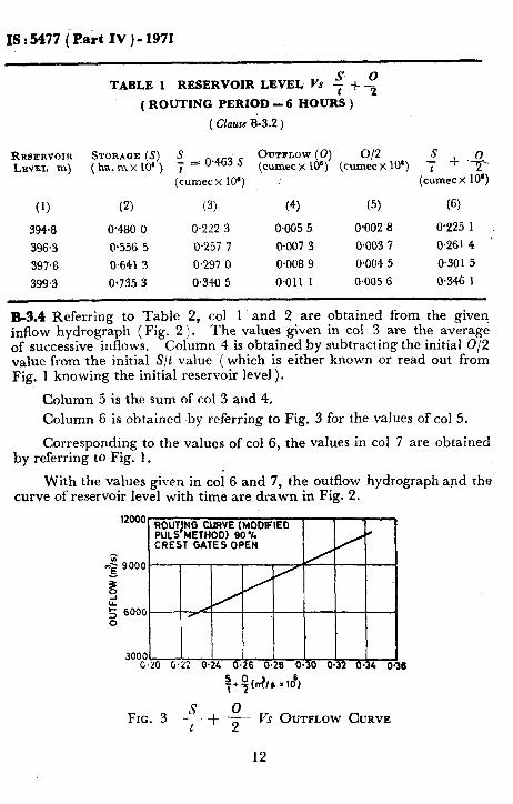
B-3.2 From Fig. 1, Table 1 is prepared.

B-3.3 By means of Table 1, Fig. 3 is prepared.

1-l

IS : 5477 ( Part IV ) - 1971

TABLE 1 RESERVOIR LEVEL k’s $ + -$

( ROUTING PERIOD - 6 HOURS )

( Clause i-3.2 )

RESERVOIR STORAGE (S) S =Oa463s OuTFLoW o/2

LEVEL m) (ha.a.X106) t (cumec x 1O8) (cumec X lo@)

(cumecx lOa) (cumecX 10’)

(‘1 (2) (3) (4) (5) (6)

394.8 0.480 0 0.222 3 0.005 5 0.002’8 0.225 1

’ 396.3 0.556 5 O-257 7 0007 3 0.003 I 0.261 4

397.8 0,641 3 0.297 0 0.008 9 0.004 5 0.301 5

399.3 0.735 3 0.340 5 0.011 1 0.005 6 0.346 1

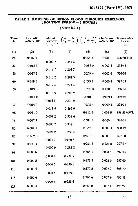
B-3.4 Referring to Table 2, co1 1 and 2 are obtained from the given inflow hydrograph (Fig. 2 ). The values given in co1 3 are the average of successive inflows. Column 4 is obtained by subtracting the initial 012 value from the initial S/t value ( which is either known or read out from Fig. 1 knowing the initial reservoir level).

Column 5 is the sum of co1 3 and 4.

Column 6 is obtained by referring to Fig. 3 for the values of co1 5.

Corresponding to the values of co1 6, the values in co1 7 are obtained by referring to Fig. 1.

With the values given in co1 6 and 7, the outflow hydrograph and the curve of reservoir level with time are drawn in Fig. 2.

FIG. 3 $ + -& Vs OUTFLOW CURVE

12

IS : 5477 ( Part IV) - 1971

TABLE 2 ROUTING OF DESIGN FLOOD THROUGH RESERVOIR ( ROUTLNG PERIOD - 6 HOURS )

( Clause B-3.4 )

TIME h

INFLOW

d/s x 1oa

m

(1)

26

32

38

44

50

(3) (4)

52

68

74

80

86

92

(2)

O-007 1

0.012 3

0.017, 1

0.019 3

0.019 6

0’018 2

0.014 9

o-011 0

o-007 4

0.004 1

0.002 3

O*OOl 1

0.009 7 0,252 3

0.014 7 0.254 7

0.018 2 O-261 5

0.019 4 0.271 4

0.018 9 0.282 2

0016 5 0.291 9

0.013 0 o-299 0

0.009 2 O-302 4

0.005 7 0.302 1

0.003 2 0.298 4

0.001 7 0.289 5

0~000 9 0.285 2

(5)

O-261 4

0.262 0

O-269 4

0.279 7

O-290 8

o-301 1

0.308 4

0.312 0

O-311 6

0.307 8

O-301 6

0.291 3

98 OaKI 6 0.286 1

0.000 6 0.277 7

104

110

116

O-000 5

OaO 4

o*oOO 4

o&O 4

O-278 3 o*ooo 5

0.000 4

OaOO 4

0.270 3

01270 8

0~263.0

O-265 4

0’256 4

122 0.256 8

(6) (7)

0.007 1 396.30 FRL

0.007 3 396.42

0.007 6 -39676

0.008 1 397.14

0.008 6 397.59

0.009 1 397.98

0.009 5 398.2 1

O-009 6 398.3 1MWL

0.009 6 398.28

0.009 4 398.19

0.009 1 397.98

0.008 8 397.67

0.008 4 397-43

0.008 0 397.09

0.007 7 396.79

3.007 4 396.58

O-007 1 396.22

L

13

IS : 5477 ( Part IV ) - 1971

APPENDIX C ( C&se 5.2)

GRAPHICAL (SORENSEN’S) METHOD OF RESERVOIR FLOOD ROUTING FOR FIXING MAXIMUM

WATER LEVEL

C-l. BASIC DATA REQUIRED

C-l.1 The following is the basic data:

a) Reservoir level zwsus spillway capacity (outflow) (see Fig. 4), and storage capacity (see Fig. 4 );

b) Full reservoir level; c) Inflow hydrograph (see Fig. 5A); d) Initial outflow; and

e) Initial storage (or initial reservoir level).

C-2. BASIC EQUATION FOR ROUTING FLOOD THROUGH RESERVOIR

C-2.1 Basic equation for routing flood through reservoir is given below:

d,.Y= (Z-O) df . . . . . . . . . . ..(7)

where dS = change in reservoir storage,

Z= rate of inflow,

0 = spillway discharge rate (or outflow rate \, and dt = time interval.

As the inflow is a function of time and outflow is a function of storage, equation (7) may be written as:

s = Sf - sj = [

i _ L!?-tOI)_ 2 1 at . . .

where 7 is the average inflow for the period At and the subscripts ‘i’ and ‘f’ refer to the initial and final conditions of the period at.

C-3. PROCEDURE

C-3.1 For graphical solution, equation (8) is transposed as follows:

( si+ y) + (i-oi ) at=s,+o,-y . ..(9)

14

IS : 5477, ( Part Iv ) - 1971

239.25 I 1 I I I I 4 l-25 2.50 3.75 5.00 6.25 7.50 6.75

(SISTORAGE (1000 ha.m) .~. L

0 0.25 0.50. 0.75 l-00 1.25 l*ko (O)OUTFLOW(lOOO ha.m PER h)

FIG. 4 RESERVOIR LEV-EL Vs STORAGE AND OUTFLOW CURVES

A constant value of A t is selected, depending on the shape of the

inflow hydrograph (here A t = 1 h ). The values of S + OAt - are plotted 2

as a function of (a) reservoir level as shown in Fig. 5B, and (b) spillway discharge (or outflow ) ps shown in Fig. 5C.

NOTE -The scales for the ordinates ofFig. 5A and 5C should be the same.

OAt In Fig. 5C by the side of S + 2 versus outflow curve, a line A is

drawn with the same origin such that its slope is --&- where C is the

ratio Of S + OAt -scale to the 0 scale ( that iqratio of the scale of X-axis

to the Y-axis o?Fig. 5C ).

c

15

IS : 5477 ( Part IV ) - 1971

For this particular example, A t is taken as one hour and the scale

ratio works out to 1 250 250= 5, which determines the slope of the line A.

At 0800 h the reservoir inflow and the outflow are known. To deter- mine the reservoir level one hour later, that is at 0900 h, the following procedure is adopted:

4

b)

c>

4

4

f 1

Draw a horizontal line a from the value of the average inflow 7 for the period 0800 h to 0900 h, towards Fig. 5C.

Draw a line b in Fig. 5C parallel to line A, from the intersection of horizontal (towards Kg. 5C) corresponding to the initial out-

OAt flow at 0800 h and the curve of S + 2 versus 0 in Fig. 5C.

The intersection point of lines a and b is projected vertically in Fig. 5B and 5C to get the points Yand Xrespectively.

The point Y of Fig. 5B is projected horizontally to Fig. 5D to get the reservoir elevation at 0900 h.

The point X of Fig. 5C is projected horizontally to Fig. 5A to get the outflow 0, at 0900 h.

With new reservoir level and outflow values as initial conditions the steps a to e are repeated for the next hourly increment. Thus reservoir stage hydrograph Fig. 5D and the outflow hydrograph Fig. 5A ( superimposed on the inflow hydrograph) are obtained.

The curves of Fig. 4 are not directly involved in the graphical solu- tion but are~the basic data for plotting Fig. 58 and 5C (see Table 3).

TABLE 3 COMPUTATION OF VALUES FOR l&g. 5B AND 5C ( WITH AI AS 1 HOUR )

ELEVATION m

(1) (2) (3) (4) (5)

240.70 I.500 0,032 0.016 1’516

242.25 2*100 0,120 0.060 2.160

243.02 2.500 0.200 0.100 2.600

243.80 3’237 0,302 o-151 3.388

245.35 5.188 O-612 0.306 -5494

246.90 7,500 0.987 0,494 7.994

STORAQE, S 1 000 ha. m

OUTFLOW, O- OAt 1000 ha. m/h - 2

I 000 ha. m

OAt s+ 2-

1 000 ha. m L

16

As in the Original Standard, this Page is Intentionally Left Blank

IS : 5477 ( Part IV ) - 1971

APPENDIX D (Clausi A-2.2 )

ESTIMATION OF PARAMETERS OF GUMBEL’S EXTREME VALUE DISTRIBUTION AND DETERMINATION OF PEAK

FLOW OF LONG TERM RETURN PERIOD

D-l. MAGNITUDE OF PEAK FLOW OF A GIVEN RETURN PERIOD

D-l.1 Gumbel postulated the use of extreme value distribution

-a(%-U) F(x)& = ae-+-u)e-e dx . . . . ..(iO)

where a and u are to be evaluated from n years annual observed peak flow values xl, x2, x3 ,............“......... .‘..........“.......) xn. Peak floy magnitude XT of T years return period is evaluated from

XT = u - (l/a) log, loge T/( T - 1 ) 2.302 6 l-

=u-- - -- u

0.362 3 + logro log10 -T_ , 1 ;..(ll)

D-2. EXAMPLE D-2-1 A worked out example for data of Sabarmati at Dharoi ( 1935 - 52 ), as given in Table 4 illustrates the computational procedure ( 1 ma/s ‘= 1000 l/s ).

Referring to Table 4,

mean flood =z = --g$.= L$? = 98.352 g ... . ..( 12)

Standard deviation s is given by 2x8 - (Z X)”

$= 2‘ (x-ZJB n

n-l 256 002 - 164446.11;6- L 5 ,22.242 650

. . . . ..( 13)

=

:. s = 75.645 50Q6

Computation for ‘a’

As a first approximation to a, take

al =Fr x _+= 0.016955 . . . . ..( 14)

Then co1 5 in Table 4 is completed. For an, as, ar, etc, of co1 6, 7 and 8 of Table 4, a step-by-step method of computing successive approximations ak + 1 from ak is given in Table 5, which is self-explanatory. Successive approximations are continued in Tables 4 and 5 till a negligibly small

‘value approaching 0 of hk is reached in Table 5. .

19

fSr5477(PareIV)-1971

(1)

YEAR

(2) 1935 1936 1937 1938 1939 1940 1941 1942 1943 1944 1945 1946 1947 1948 1949 1951 1952

TABLE 4 VALUE OF c-az

( Clause D-2.1 )

PEAK FLOW

RATE (x)

‘:;y I

(3)

76

ld

2:; 91

:s 193 246 187

z 20 48

102 6

,-V e -a,p ,-v 4

-laoa

(4) (5) (6) (7) (8) 5 776

15 62: 6 241

51 529 8 281 1 764

15 625 37 249 60 516 34 969 2 025 3 249

2% 10 404

36

0.275 7 0.263 1 0262 4 0262 4 0.950 4 0948 6 0.948 6 0.948 6 0.120 1 0.1113 0.110 8 0.110 8 0.262 0 0.249 7 0249 0 0.249 0 0.021 3 0.018 6 0.018 4 0018 4 0,213 7 0.202 2 0.201 6 0.201 5 0.490 6 0.478 2 0.477 4 0.477 4 0.120 1 0.111 3 0.110 8 0.110 8 0.037 9 0033 7 0.033 5 0033 5 o-015 4 0.013 3 0.013 2 @013 2 0.042 0 0.037 5 0.037 2 0.037 2 0466 2 0.453 6 0.452 9 0’452 9 0.380 5 0,367 5 0.366 7 0366 7 0.712 4 0.703 7 0.703 3 0.703 3 0.443 2 0.430 3 0429 6 C.429 6 0.177 4 0.166 6 0.166 1 0.166 I 0.903 3 0.899 9 0,899 7 0899 7

TOTAL 1672 256 002 5.632 2 5489 1 54812 5.481 1

,Computation for ‘IO

From the steady value so reached of ak for k = 4 (in the present case ), compute

u= logslOX -$ C

log10 (n)--loglo (Ze -akzi ) 1

= 64.297 104

. ..( 15)

Putting these values of I( and the steady ok in ( 11 ), expected peak values %r for T = 50; 100; 200; 500, etc, years return periods are evaluated as

~6s = 285.97; xlw = 325.63; xzoo = 365.15; ~500 = 417.30

In order to safeguard against incidental errors of estimation arising from small samples of 29, 30, ..‘.......... _., years observed data available the above best estimates may be increased by I.645 SE(xr ) to warrant 95 percent dependability of the design estimates. The standard error of

. 20

L

IS : 5477 (Part IV ) - 1971

estimation $E( XT ) is given by

SE( XT ) = a :-;;-[I + -$-{ l-O.577216

--log, loger/(z--1) . . . . ..(16)

1 = ___ 1 + 0.607 927 1

a&- [

-log,logeT/(2--1) . . . . ..(17)

Thus

x60-= 2 859 700 l/s ( = 2 859.7 ma/s) + 797.3 ms/s

x100 = 3 256 300 ,, ( = 3 256.3 ma/s) + 916.1 ma/s

xzoo = 3 651 500 ,, ( = 3 651.5 ms/s) + 1035.7 ms/s

xsoo = 4 173 000 ,, ( = 4 173.0 ma/s) + 1 194.6 ma/s

Values of A = --log, loge T/( T- 1 ) for the most commonly used values of T like 20, 50, 100, 200,50@,.and 1000 years are reproduced below for convenience of users:

l-=20 50 100 200 500 1000

A ~2-9702 3.9020, 4.6002 5.2958 6.2137 6.9073

D-2.2 It is advisable to procure always at least 20-25 years observed records and not to compute estimates for return periods longer than about 20n or 2% years.

D-2.3 The steps remain very much the same irrespective of the value of n, the number of years. Though the computational steps by successive approximation method appear very arduous, their schematically outlined procedure as in D-2.1, even with recorded data of around 50 years should not take a person equipped with an ordinary calculating machine and a book of logarithm tables more than 6-7 hours. With electronic fast computers the stabilized expression can be secured in two to three minutes for which programme is given in D-3. L

D-2.4 The calculation of a 500 years ’ flood, for example does not tell when the flood is coming; it might occur in any year within that period or not until 500 years have elapsed.

D-2.5 The choice of a suitable return period on which to base the ‘design flood’ is the engineer’s responsibility, and rests ultimately on his judgement and experience. The size and cost of the dam, the design freeboard, the amount of water stored, and the likely consequences of failure are factors which influence the selection.

21

STEP QVANRTY k=l k-2 k=3

6

7

8

9

10

11

12

- =tic z Xi6

- wd z 2‘8

f (0,) = (7) - (5) (6)

f’ bk) = (8) + (5) (7) - (4) (6)

01: + , = ok + hk I

TAlriLE 5 FOR VALUES OF @k + I &?koht #k

k=4

0.016 955 0.017 565 0.017 602

0.007 363 0’007 628 0+07 644

58.979 6 56.931 4 56.811 7

3 478.593 2 3 241.184 3 3 227.569 3

39.373 3 41.421 5 41.541 2

0.017 602 58 b

0*007 645 2

56.809 9

3 227.364 7

41.543 0

5.632 2 5489 1 54812 54811

240.075 2 228.368 4 227.711 1 227.702 0

19 898.861 8 18 563.741 2 18 488.027 9 18 487.199 8

18.316 900 lflOl644 oa15 475 Of@0 663

-30 038++15 -26 895.564 3 -26 719588 4 -26 717.284 3

0.000 610 omo 037

0.017 602

Of)00 000 58 0.000 000 02

0.017 565 0.017 602 58 0.176 026 0

( Clause D-2.1 )

c

IS : 5477 (Part IV) - 1971

D-3. COMPUTER PROGRAMME FOR PEAK FLOOD ESTIMA- TION BY MAXIMUM LIKELIHOOD METHOD

FIRST DATA CARD IS NO. OF OBSERVATION 4COLS, NAMES OF RIVER, SITE, UNIT OF OBSERVATION 8COLS EACH FOLLOWED BY DATA CARDS 4COLS EACH OBSERVATION. ~;~E~;ION X( 100 ), EX( 100 )

SQS&O. READ 2, N, RVR, SITE, UNIT

2 FORMAT ( 14,3A8) READ3, ( X (I), I=l, N )

3 FORMAT (20F4.2) D05I=I,N SUM=SUM+X(I)

5 ;QS$M=SQSUM+X(I)**2

SQSUM=(SQSUM-SUM*SUM/B)/(B-1.) SUM=SUM/B T=3.141592654 &%;/SQRTF(6.*SQSUM)

DO i.j=l, 20 SIG=O. XSIG=O. XZSIG=O. A=A-H -tiO-8 I=l, N

EX( I ) =EXPF(-A*X(I)) SIG=SIG+EX(I) XSIG = XSIG + X( I )*EXf I 1 XZSIG = X2SIG + Xc’1 )*X( f)*EX( I ) FA = XSlG - ( SUM - 1./A )*SIG FH = ( SUM - 1,/A )fXSIG - XZSIG - SIG/A**2 H = FA/FH IF(ABSF(H)- l.E - 06 ) 30, 30, 1 CONTINUE

30 ;I: T ;A/( T**2 )

U= T*LoGF( B/sxG ) X20 = U + T*2.970186 X50 = U + T*3.901953 xl00 = U‘+ T*4.600150 X2nO = U + T*5.295775 X500 = U + T*6.213675 t’ c l./( A*SQRTF ( B ) ) SEX20 = P*SQRTF ( 1. + PIE*( 0.422784 + 2.970186)**2 ) SEX50 = P*SQRTF ( 1. + PIE*( 0.422784 + 3.901953 )**2 ) SEX100 = P*SQRTF ( 1. + PIE*( 0.422784 + 4.600150)**2) SEX200 = P*SQRTF ( 1. + PIE*( 0.422784 + 5.295775 )**2 ) SEX500 = P*SQRTF ( 1. + PIE*( 0.422784 + 6.213675 )**2 ) PRINT 310, UNIT, RVR, SITE

23

IS:%77 (Part IV)-1971

310 1

309 1

311

312

FORMAT(IH1/////30X 43HEXPECTEDVALUES WITH VARIOUS RETURN Pm101 46X, IH*, A8, 4X, lH*//4OX, A8,3X,2HAT,A8) PRlNT !-4W _ _--_. _ __I

FORMAT( //29X. 8H20 YEARS, 12X, 8H50 YEARS, 11X, 9HlOO YEARS, IIX, 9H2( EARS, 11X, 9H500 YEARS) PRINT 311, X20, X50, X100, X200, X500 FORMAT( 8X. SHESTIMATE -, 5 ( 4X. F16.9 ) ) PRINT 312, SEXBO, SEX50, SEXlOO, SEX200. SEX500 FORMAT( /9X, 8HSTD ERR =, 5 ( 4-X, F16.9 ) ) STOP END

24