Irreversible thermodynamics, - Startsidaweb.abo.fi/~rzevenho/PET15-5-IRR.pdf · Irreversible...

8.2.2015Åbo Akademi Univ - Thermal and Flow Engineering Piispankatu 8, 20500 Turku 1/32

Irreversible thermodynamics, a.k.a. Non-equilibrium thermodynamics(an introduction)

Ron ZevenhovenÅbo Akademi University

Thermal and Flow Engineering Laboratory / Värme- och strömningstekniktel. 3223 ; [email protected]

Process EngineeringThermodynamicscourse # 424304.0 v. 2015

ÅA 424304


5.1 Equilibrium, classicalthermodynamics vs.irreverisible (non-equilibrium)thermodynamics


Irreversible thermodynamics /1

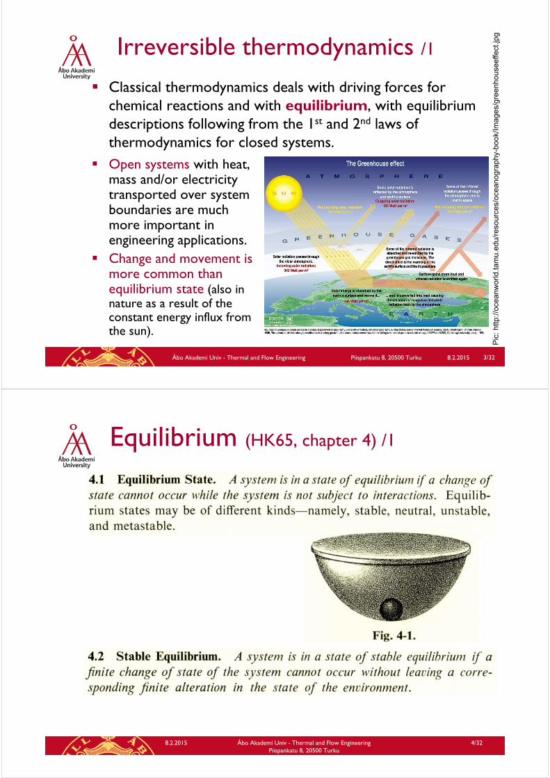
Classical thermodynamics deals with driving forces for chemical reactions and with equilibrium, with equilibriumdescriptions following from the 1st and 2nd laws of thermodynamics for closed systems.

Open systems with heat, mass and/or electricitytransported over system boundaries are muchmore important in engineering applications.

Change and movement is more common thanequilibrium state (also in nature as a result of the constant energy influx from the sun).

Pic

: ht

tp://

ocea

nwor

ld.ta

mu.

edu/

reso

urce

s/oc

eano

grap

hy-b

ook/

Imag

es/g

reen

hous

eeffe

ct.jp

g

8.2.2015 Åbo Akademi Univ - Thermal and Flow Engineering Piispankatu 8, 20500 Turku

4/32

Equilibrium (HK65, chapter 4) /1


5/32

Equilibrium (HK65, chapter 4) /2



Irreversible thermodynamics addresses non-equilibrium situations, assuming reversibilityon a small scale (i.e. local equilibrium) and linear transport processes.

A starting point was the work of Thomson (later Lord Kelvin) on thermo-electricity, i.e. interacting transport of heat and electric charge in the 1850’s

The main goal is to describeinteracting transport processes, taking into accountentropy production and the 2nd Law of thermodynamics

An Estonian-German physicist Thomas Seebeck (1770-1831) twisted two wires of different metals together and heated the point at where they were joined. He produced a small current of electricity. This is called thermo-electricity and is known in physics as the "Seebeck Effect". P

ic: h

ttp://

ww

w.w

orld

ofen

ergy

.com

.au/

07_t

imel

ine_

wor

ld_1

812_

1827

.htm

l


7/32

Transport processes (linear) /1

Entropy production and Fourier’s law:

force driving coeff. transportflux :general in

: :

: :

ii

yxymmI

MQ

XLJdx

dvJNewton

dx

dV

A

iJOhm

dx

dcD

A

nJFick

dx

dT

A

QJFourier

2

22

222

ba

:lossexergy

:T and T betweenfer Heat trans

dx

dT

T

T

volume

xEΔ

T

TAJTSTxEΔ

T

TAJ

T

TQ S

dt

dS

T

TdQ

TT

TTdQdS

o

Qo

geno

Qgengen

ba

bagen

A m2

(voltage V, specif. conductance σ = 1/ρ, where spec. resistance ρ = R∙A/Δx)

dx

R = electricalresistance, Ω


8/32


Similar for electric current (or mass diffusion or fluid flow):

This gives the general description Ji = L·Xi, and

Cross-effects and interactions can be described too:

2

:loss exergy *

dx

dV

T

T

volume

xEΔ

T

ViTSTxEΔ

T

Vi

dt

dSS

dt

dSTViQ

oo

geno

gen

TVΔ

X,iJ:Ohm;TTΔ

X,JJ:Fourier

JX;XJS

iiiQi

iiiigen

and and

for force driving the is where

relations) reciprocal s(Onsager' L Lwhere

and ;

jiij

22212122121111

XLXLJXLXLJ

V =voltage

flows heat

or mass no *

dt

dSSgen


9/32


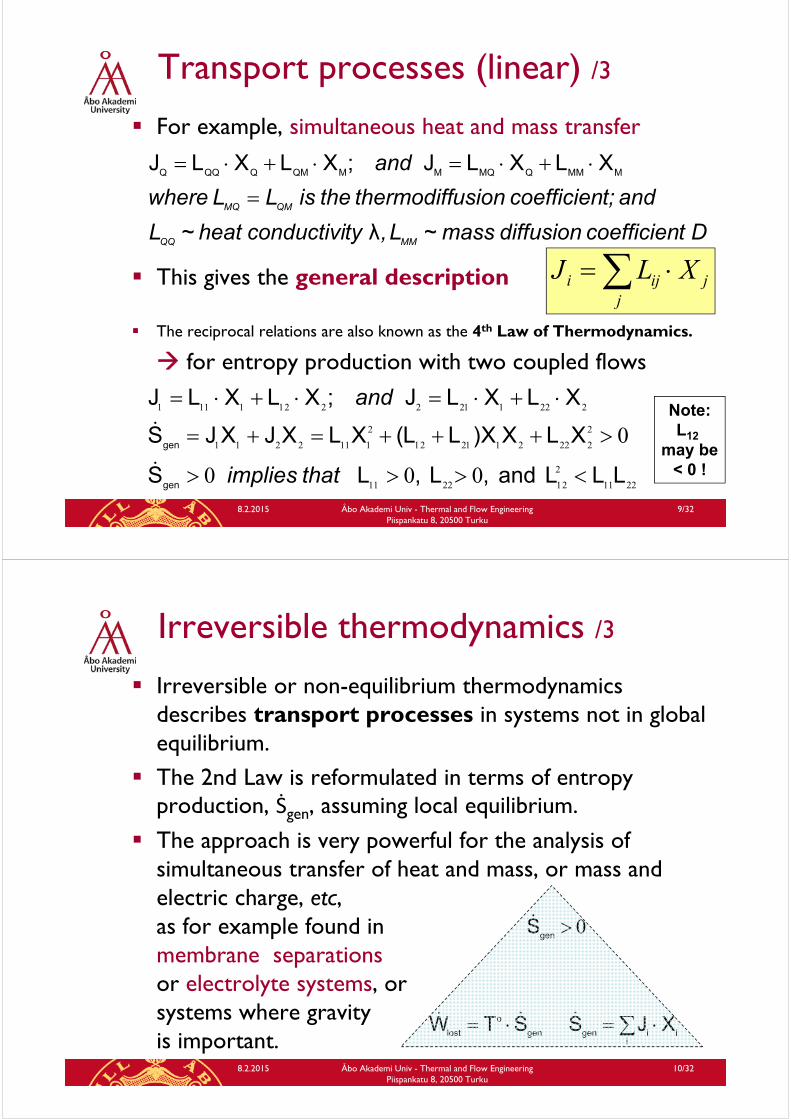
For example, simultaneous heat and mass transfer

This gives the general description

The reciprocal relations are also known as the 4th Law of Thermodynamics.

for entropy production with two coupled flows

D tcoefficien diffusionmass ~ L , tyconductivi heat ~ L

and t;coefficien usionthermodiff theis LL where

and

MMQQ

QMMQ

λ

XLXLJ;XLXLJMMMQMQMMQMQQQQ

j

jiji XLJ

LLLand,L,LS

XLXX)LL(XLXJXJS

XLXLJ;XLXLJ

gen

gen

thatimplies

and

Note:L12

may be< 0 !


10/32


Irreversible or non-equilibrium thermodynamicsdescribes transport processes in systems not in global equilibrium.

The 2nd Law is reformulated in terms of entropyproduction, Ṡgen, assuming local equilibrium.

The approach is very powerful for the analysis of simultaneous transfer of heat and mass, or mass and electric charge, etc, as for example found in membrane separationsor electrolyte systems, or systems where gravityis important.

iiigengen

o

lost

gen

XJSSTW

S


11/32

Driving forces; entropy production For heat exchange the entropy production rate is the

product of the thermodynamic driving force X = Δ(1/T) and the resulting flow J = Q.

For more general systems, for example an isolatedsystem separated into sections by a membranepermeable only to one species (e.g. species ”1”):

iii

gen

gen

XJ

T

µn

T

pV

TQS

T

µ

T

µ

dt

dn

T

p

T

p

dt

dV

TTdt

dQ

dt

dS

111

2

2

1

11

2

2

1

11

21

1

1

11

V1, n1,p1,T1, µ1

V2, n2,p2,T2, µ2

.


An example

Source:K07

zT

yT

xT

T

andvolume

S

Here

gen

/

/

/

:

ÅA 424304


5.2 Maximum entropy production


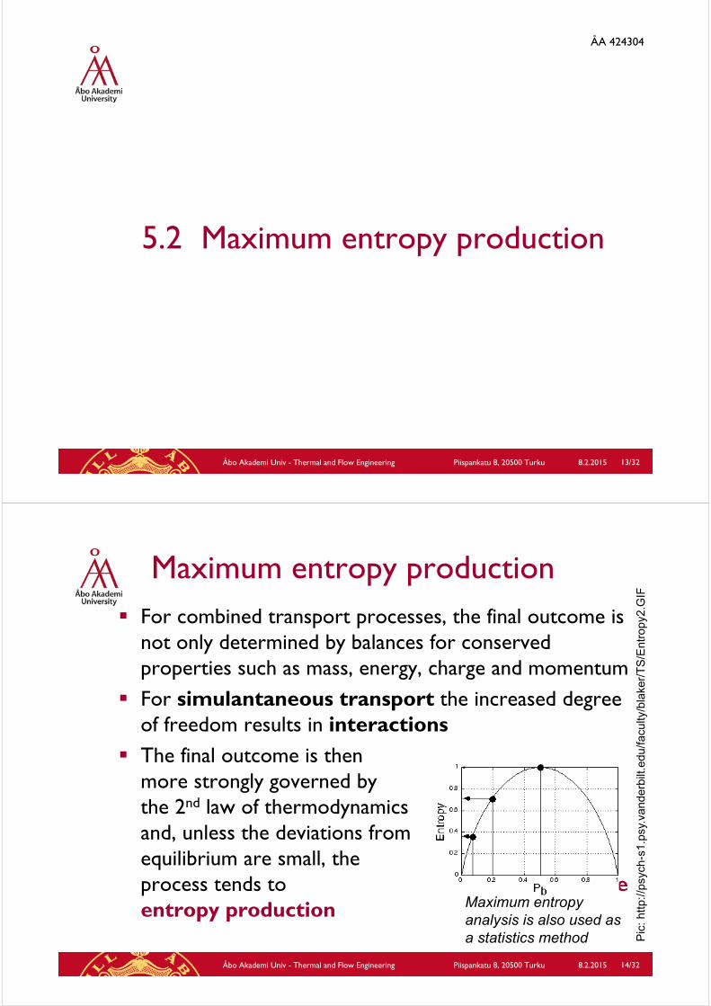
Maximum entropy production For combined transport processes, the final outcome is

not only determined by balances for conservedproperties such as mass, energy, charge and momentum

For simulantaneous transport the increased degreeof freedom results in interactions

The final outcome is thenmore strongly governed by the 2nd law of thermodynamicsand, unless the deviations from equilibrium are small, the process tends to maximiseentropy production Maximum entropy

analysis is also used asa statistics method P

ic: h

ttp://

psyc

h-s1

.psy

.van

derb

ilt.e

du/fa

culty

/bla

ker/

TS

/Ent

ropy

2.G

IF


Max. entropy production example/1

An electric heating element distributes heat Q intoQ1+ Q2 while heating up two different streams. Input energy Q results in temperature Th for the heating element. The system is well insulated.

For both streams the energy balance equation gives Qi= ṁi·ΔTi·cpi = Ui·Ai·ΔTlm,i, and Q = Q1 + Q2 is fixed. (Assume A1 = A2, or even U1·A1 = U2·A2).

How will the input heat energy Q be distributed?

T=ThHeat Q

Flow ṁ1, T1, cp1

Flow ṁ2, T2, cp2

Q1

Q2

Flow ṁ2, T4, cp2

Flow ṁ1, T3, cp1


16/32


For one of the streams the entropy generation is

The result follows from max {Ṡgen1(Q1) + Ṡgen2 (Q2)}

T=ThHeat Q

Flow ṁ1, T1, cp1

Flow ṁ2, T2, cp2

Q1

Q2

Flow ṁ2, T4, cp2

Flow ṁ1, T3, cp1

stream other the for similar also while

;cm

QTT

)TT

ln(cmT

dTcmdT

T

cmdSS

,p

,p

T

T,p

T

T

,pT

T,gen


17/32


Thus,

which can be solved for Q1, giving Q2= Q - Q1, finally giving temperatures T3 and T4.

T=ThHeat Q

Flow ṁ1, T1, cp1

Flow ṁ2, T2, cp2

Q1

Q2

Flow ṁ2, T4, cp2

Flow ṁ1, T3, cp1

)QQ(Tcm

cm

QTcm

cm

,dQ

Sd

dQ

Sd

,p

,p

,p

,p

,gen,gen

gives which

ÅA 424304


5.3 Thermo-electricity


19/32

Entropy generation /1

Consider a slice of a material that conduct heat and electricity; the heat flux Ф” (W/m2) and electriccurrent density I” (A/m2).

The entropy production rate per unit volume (area·dx) ds’’’/dt for the heat flow is given by

V= electric potentialT = temperature

Pic, source: B01


20/38


Pic, source: B01

see alsonext slide

See alsoslides 7,8

T

dV

dx

''idtvolume

ds

dt

'''ds

Then for the total volume A·dx:

For the electric current density (Ohm’s law):with σ = 1/ρ, with specific electrical resistance ρ

The entropy production as a result of Ohmic losses, per unit volume:


21/32


Then for the total volume:

The processes can be coupled using:

with

Pic, source: B01

)R( resistance with Ω

dxdV

Tσ

TσI

dxTdxρIdxT

dRareaIdxareaT

dRIvolumeT

Qddt

'''ds

:Note

''''

''


22/38


Pic, source: B012

22

2112

211

222

21

T

dT

L

LL

T

dTLΦ

T

dT

L

LT

dV

0I

R

dVT

dVL

I

0dT

22

According to Ohm’s law, if dT = 0:

with resistance R = ρ·dx/A, for thickness dx, area A

Fourier’s law follows from I = 0: with Φ = G∙dT, heat conductance G = λ·A/dx.

A third material property is needed to describe the cross phenomena: the Seebeck coefficient, θ, defined as:


23/38


This gives for current I: Eliminating the voltage gradient dV/dx from the

expressions gives

which with conductance G = λ·area/dx can also be written as

combining Fourier’s law and the Seebeck effect.

Pic, source: B01

thermo-electricity


The Seebeck effect

For combined heat flow and electric current, with I = 0:

This means that the voltage difference ΔV (”thermo-current”) for the system in the Fig. can be can be calculated as:

Δ

Δ

Reference temperature

Thermometry , i.e. a thermocouple Pic, source: B01


The Peltier effect /1

Consider again combined heat flow and electric current, but now with dT = 0. The Onsager expressions nowgive: and

Combining dT = 0 with gives

which implies that an electric current involves a heat flow as well, which enters and leaves the material without causing heating or cooling.

Pic, source: B01


The Peltier effect /2

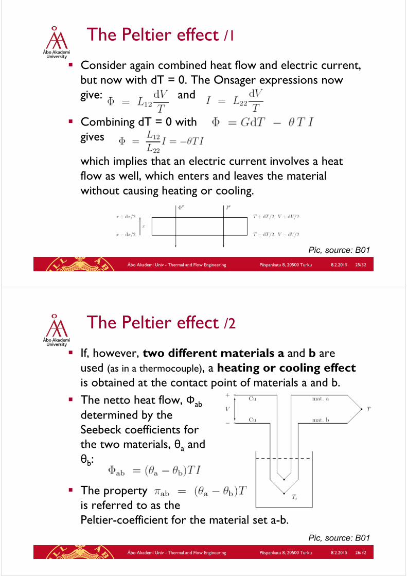
If, however, two different materials a and b are used (as in a thermocouple), a heating or cooling effectis obtained at the contact point of materials a and b.

The netto heat flow, Фab is determined by the Seebeck coefficients for the two materials, θa and θb:

The propertyis referred to as the Peltier-coefficient for the material set a-b.

Pic, source: B01

ÅA 424304


5.4 Power from osmosis


28/32

The mixing of sea water with fresh water gives a (mixing) exergyeffect that can be exploited

Installing a membranesystem at 120-150 m below the fresh water intake allows for a significant extra hydropower effect

Pic, source: KB08

Work from a saline power plant /1


29/32

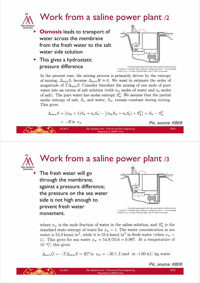
Osmosis leads to transport of water across the membranefrom the fresh water to the salt water side solution

This gives a hydrostaticpressure difference

Pic, source: KB08



30/32

The fresh water will go through the membrane, against a pressure difference; the pressure on the sea water side is not high enough to prevent fresh water movement.

Pic, source: KB08



31/32

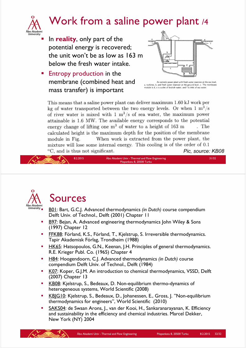
In reality, only part of the potential energy is recovered; the unit won’t be as low as 163 m below the fresh water intake.

Entropy production in the membrane (combined heat and mass transfer) is important


Pic, source: KB08


Sources B01: Bart, G.C.J. Advanced thermodynamics (in Dutch) course compendium

Delft Univ. of Technol., Delft (2001) Chapter 11 B97: Bejan, A. Advanced engineering thermodynamics John Wiley & Sons

(1997) Chapter 12 FFK88: Förland, K.S., Förland, T., Kjelstrup, S. Irreversible thermodynamics.

Tapir Akademisk Förlag, Trondheim (1988) HK65: Hatsopoulos, G.N., Keenan, J.H. Principles of general thermodynamics.

R.E. Krieger Publ. Co. (1965) Chapter 4 H84: Hoogendoorn, C.J. Advanced thermodynamics (in Dutch) course

compendium Delft Univ. of Technol., Delft (1984) K07: Koper, G.J.M. An introduction to chemical thermodynamics, VSSD, Delft

(2007) Chapter 13 KB08: Kjelstrup, S., Bedeaux, D. Non-equilibrium thermo-dynamics of

heterogeneous systems, World Scientific (2008) KBJG10: Kjelstrup, S., Bedeaux, D., Johanessen, E., Gross, J. ”Non-equilibrium

thermodynamics for engineers”, World Scientific (2010) SAKS04: de Swaan Arons, J., van der Kooi, H., Sankaranarayanan, K. Efficiency

and sustainability in the efficiency and chemical industries. Marcel Dekker, New York (NY) 2004

Irreversible thermodynamics, - Startsidaweb.abo.fi/~rzevenho/PET15-5-IRR.pdf · Irreversible...

Documents

Transcript of Irreversible thermodynamics, - Startsidaweb.abo.fi/~rzevenho/PET15-5-IRR.pdf · Irreversible...