Irish Sustainable Development Model (ISus) Literature ...

www.esri.ie

Working Paper No. 186 February 2007

Irish Sustainable Development Model (ISus) Literature Review, Data Availability and Model Design

Joe O’Doherty Karen Mayor

Richard S.J. Tol

ESRI working papers represent un-refereed work-in-progress by members who are solely responsible for the content and any views expressed therein. Any comments on these papers will be welcome and should be sent to the author(s) by email. Papers may only be downloaded for personal use only.

http://www.esri.ie/

Contents

1. Introduction 5

2. Environmental Processes 7

2.1 Eutrophication 7

2.1.1 Issue 7

2.1.2 Effect 7

2.1.3 Prevention and mitigation 7

2.1.4 Situation in Ireland 8

2.2 Climate change 8

2.2.1 Issue 8

2.2.2 Effect 8



2.3 Acidification 10

2.3.1 Issue 10

2.3.2 Effect 10



2.4 Air quality 12

2.4.1 Issue 12

2.4.2 Effect 13



2.5 Resource use 15

2.5.1 Issue 15

2.5.2 Effect 15



2.6 Waste 17

2.6.1 Issue 17

2.6.2 Effect 17



2.7 Conclusion 19

3. Modelling the environment 20

3.1 Emission models 20

3.1.1 Decomposition 20

3.1.2 Environmental Kuznets Curve (EKC) analysis 22

3.1.3 Input-Output models 23

3.1.4 Computable General Equilibrium (CGE) models 24

3.1.5 Econometric models 27

3.1.6 Optimisation and partial equilibrium (“optimal control”) models 28

3.1.7 Hybrid models 31

3.2 Land Use Models 35

3.2.1 Land use in economics 35

3.2.2 Geographic models of land use 36

3.2.3 Economic models of land use 36

3.3 Conclusion 37

4. Environmental valuation 38

4.1Valuation theory 38

4.1.1 Hedonic pricing 38

4.1.2 The Travel Cost Method 39

4.1.3 Contingent valuation techniques 39

4.1.4 Choice modelling 40

4.2 In practice – Valuation studies conducted in Ireland 40

4.2.1 Rivers, Water and recreation 40

4.2.2 Agriculture 41

4.2.3 Forests 42

4.3 Conclusion 43

5. Indicators and data 44

6. The Sustainable Development Research Model: Design Issues 49

6.1 Activities in other countries 49

6.1.1 UK 49

6.1.2 Netherlands 49

6.1.3 Switzerland 50

6.1.4 France 50

6.1.5 Germany 50

6.1.6 Belgium 50

6.1.7 European Union 51

6.1.8 OECD and IEA 51

6.1.9 UN 51

6.2 Model Design 52

7. Conclusion 62

Acknowledgements 64

8. Appendix 65

9. Bibliography 69

3

List of Figures

2.1 Effects of acid rain on a forest and a sculpture 11

2.2 Seasonal mean black smoke and sulphur dioxide concentrations, September 1984-96 14

2.3 Fixed air monitoring stations in Ireland 14

2.4 World oil production capacity 16

2.5 The waste hierarchy 18

2.6 Waste generation in Ireland and principal sources – 2001 18

2.7 Impact of policy on – and relative importance of – environmental problems 19

3.1 Typical shape of the Environmental Kuznets Curve 22

3.2 Overview of the MERGE model 31

3.3 Overview of the CETA model 32

3.4 Overview of the SGM model 33

5.1 Aggregation and information pyramids 45

6.1 Structure of ISus0.0 59



List of Tables

3.1 Four models for calculating SNI 26

4.1 Summary of results from choice experiments 41

5.1 Environmental data for the Republic of Ireland 47

5.2 Comparison of the environmental accounts of selected countries 48

6.1 Emissions in ISus 54

6.2 Resource use in ISus 54

6.3 Spatial resolution in ISus 54

6.4 Sectoral resolution in ISus 55

6.5 Emission and resource use coefficients in ISus 55

6.6 Scope of ISus 55

6.7 ISus output compared to EPA environmental indicators 55

4

Irish Sustainable Development Model (ISus) Literature Review, Data Availability and Model Design

1. Introduction

Economic growth can increase pressure on the environment. See, for example, the growth in carbon dioxide emissions in Ireland. However, when economic activity is properly managed, the associated environmental pressure can be reduced or even eliminated at low costs. Proper management requires information. Where do emissions originate? How would emissions develop over time if policy were unchanged? How would emissions respond to changes in policy? What are the interactions between different environmental policies? Is stringent environmental policy compatible with vigorous economic growth?

Answering these questions requires data and models. While the availability and quality of data on the environment in Ireland have improved markedly in the last 15 years, model development is still in an early stage. Therefore, the Environmental Protection Agency (EPA) has commissioned the Economic and Social Research Institute (ESRI) to develop a sustainable development research model for Ireland: Irish Sustainable Development Model (ISus). The model will be capable of linking economic and social developments to their related environmental impacts to provide a tool for policy-makers to assess the implications of different growth paths for national objectives on sustainable development,1 and will be used to project emissions and resources until 2025.

It was suggested in the ESRI’s tender for the ISus project that to be successful, any modelling framework needs to fulfil two criteria. Firstly, it needs to be useful to and used by key policy-makers. Secondly, it should build on models and research that are already available.

This document fulfils the second of these requirements and in so doing provides a review of the relevant literature and data sources for a sustainable development model.

Having introduced the study in this section, section two presents an analysis of six processes that currently impact on Ireland’s environment.

Section three presents an overview of existing economic models that have been used in relation to environment-economy interactions, as well as a dedicated discussion of land use modelling.

Section four presents an analysis of evaluation techniques.

Section five presents the data and indicators currently available in Ireland.

1 The Brundtland Commission (1987) defines sustainable development as ‘development that meets the needs of the present without compromising the ability of future generations to meet their own needs.’

5

Section six presents an overview of similar projects elsewhere, as well as the proposed design for the ISus model in terms of its scope, structure and applications.

The concluding section draws inferences from each of the previous sections in order to critically assess the parameters that constrain the development of a sustainable research model for Ireland.

6

2. Environmental Processes

The first step in the construction of the ISus model will be to determine what forcings are important in an Irish context, and thus what emissions should be analysed and what data should be collated. As such, this section will examine the issues surrounding six processes that impact on the environment, the effect they can have, how they can be prevented or mitigated, and – perhaps most importantly with a view to constructing the ISus model – how each of these is relevant in Ireland. The environmental processes discussed below are eutrophication, climate change, acidification, air quality, resource use and waste.

2.1 Eutrophication

2.1.1 Issue Eutrophication involves the enrichment of an ecosystem with chemical nutrients, typically compounds containing nitrogen (N) and phosphorus (P). A certain amount of eutrophication occurs naturally, particularly in aquatic environments, but this process can be accentuated by human behaviour.

2.1.2 Effect Eutrophication can have the following effects (from Carpenter et al., 1998; Smith, 1998):

• Increased biomass of phytoplankton

• Toxic or inedible phytoplankton species

• Increases in blooms of gelatinous zooplankton

• Increased biomass of benthic and epiphytic algae

• Changes in macrophyte species composition and biomass

• Decreases in water transparency

• Taste, odour, and water treatment problems

• Dissolved oxygen depletion

• Increased incidence of fish kills

• Loss of desirable fish species

• Reductions in harvestable fish and shellfish

• Decreases in perceived aesthetic value of the water body

2.1.3 Prevention and mitigation Sources of P and N that contribute to eutrophication include wastewater effluent, agriculture (particularly fertiliser application and intensive animal husbandry), irrigation and waste disposal sites. Measures to counter this problem can involve technical measures (e.g., treatment of manure and sewage), management changes

7

(e.g., application of fertilizers) and structural changes (e.g., extensification of agriculture).

2.1.4 Situation in Ireland In Ireland, water quality is not a significant problem. However, the problems that do exist in this area are generally due to eutrophication. In 2005 the European Environment Agency noted that:

‘Ireland's water quality overall remains of a high standard. Serious pollution in rivers and streams has been reduced to just 0.6 % of river channel, its lowest level since the early 1990s. Eutrophication of rivers, lakes and tidal waters continues to be the main threat to surface waters with agricultural run-off and municipal discharges being the key contributors.’

2.2 Climate change

2.2.1 Issue Climate change refers to the variation in the global climate, or in regional or national climates, over time. It can be caused by both natural factors (e.g., glaciation and plate tectonics) and human factors (e.g., emissions of greenhouse gases and aerosols, and land use changes). The ‘main greenhouse gases’ observed by the United Nations Framework Convention on Climate Change (UNFCCC) are Carbon dioxide (CO2), Methane (CH4), Nitrous oxide (N2O), Perfluorocarbons (PFCs), Hydrofluorocarbons (HFCs) and Sulphur hexafluoride (SF6) (UNFCCC, 2006).

2.2.2 Effect The effects of climate change are most notably manifest in varying weather conditions. In a special report, The Economist noted that ‘over the past 100 years [net temperatures] have gone up by about 0.6°C’ (2006a).

This rise in temperatures is predicted to accelerate by most commentators, who foresee global temperatures increasing by between 1°C and 6°C in the coming century (IPCC, 2006, 11). The effects on the environment of such a change could be significant. Rising sea levels would increase the risk of flooding and raise sea levels, placing many of the world’s low-lying areas at risk of being submerged. Declining crop yields and increased risk of disease could also affect many of the world’s warmest regions.

There are also mechanisms that act to amplify the effect of a given forcing. For example, melting ice caps can accelerate the process of further melting as the Earth’s surface absorbs more of the Sun’s heat.

2.2.3 Prevention and mitigation The view that anthropogenic factors contribute significantly to climate change has become more popular in recent years (The Economist, 2006). Mitigation of forecasted climate change is thus in many respects a human responsibility.

Two recent studies recommend action now to curb GHG emissions in the future. The Economist special report on climate change and the Stern Review on the economics of climate change differ markedly in their assessment of the costs that global warming

8

could impose on humankind.2 However, both reports recommend that action should begin now in order to minimise the effects of climate change before its effects become irreversible.

Using traditional methods, the economic evidence in favour of mitigation is relatively weak. Cost-benefit analysis generally uses a discount rate that values costs and benefits now over the future. With mitigation of climate change, a certain amount of outlay now may lead to uncertain benefits in the future. Indeed, the very fact that these benefits are uncertain counts against action on climate change according to Bjorn Lomborg, the self-titled “sceptical environmentalist”. In their survey, The Economist poses a similar question:

‘Is it really worth using public resources now to avert an uncertain, distant risk?…If the risk is big enough, yes. Governments do it all the time. They spend a small slice of tax revenue on keeping standing armies not because they think their countries are in imminent danger of invasion but because, if it happened, the consequences would be catastrophic’ (2005, 15).

In any event, Ireland is committed to greenhouse gas emission reduction until 2012 under the Kyoto Protocol, and after that date under EU climate policy.

2.2.4 Situation in Ireland A report by McGrath et al. for the EPA in 2005 sought to model the effects of climate change in Ireland. A regional climate model ‘was used to simulate the future climate for the period 2021-2060’ (McGrath, 2005, 1). The results of their research are summarised as follows:

‘Projected temperature changes from the model output show a general warming in the future period with mean monthly temperatures increasing typically between 1.25 and 1.5°C. The largest increases are seen in the southeast and east, with the greatest warming occurring in July.

For precipitation, the most significant changes occur in the months of June and December; June values show a decrease of about 10% compared with the current climate, noticeably in the southern half of the country; December values show increases ranging between 10% in the south-east and 25% in the north-west. There is also some evidence of an increase in the frequency of extreme precipitation events (i.e. events which exceed 20 mm or more per day) in the north-west.

In the future scenario, the frequency of intense cyclones (storms) over the North Atlantic area in the vicinity of Ireland is increased by about 15% compared with the current climate’ (ibid, vii)

2 The Stern Review notes that ‘the total cost of ‘business as usual’ climate change is the equivalent of around a 20% reduction in consumption per head, now and into the future’. The Economist report cites two other papers that report a range of, in the first instance, 0.1% of global output per year (Mendelsohn, 2000), and in the second instance, 2% of global output (Nordhaus, 2000) as the costs of climate change.

9

The baseline scenario used in the above model assumes ‘business as usual’ behaviour by economic actors throughout the world. The reality for Ireland is that, as a small country, domestic policies to prevent climate change will have little impact if the rest of the world continues along its ‘business as usual’ path.

Efforts to alter this path by reducing worldwide emissions of GHGs culminated in the agreement of the Kyoto protocol in 1997.3

Ireland is committed to the protocol under international law as a signatory to the Marrakech Accords – an agreement that divided the EU’s commitment to reduce overall emissions by 8% between its 25 members. Because of its recent economic growth, Ireland is permitted a 13% rise in emissions from 1990 levels. However, Ireland’s emissions are currently 10% above this allowance (23% above 1990 levels) and the government plans to buy emission permits from abroad to meet the obligations under the Kyoto Protocol (The Irish Times, 2006).

Ireland’s failure to reduce its emissions in line with its Kyoto commitments is ostensibly in conflict with government policy; the National Climate Change Strategy (NCCS) was published in October 2000 in order to provide ‘a framework for achieving greenhouse gas emissions reductions’ (DEHLG, 2000, 2).

2.3 Acidification

2.3.1 Issue Acidification refers to ‘the process whereby air pollution – mainly ammonia (NH3), Sulphur Dioxide (SO2) and Nitrogen Oxides (NOx) – is converted into acidic substances’ (EEA, 2006). The term ‘acid rain’ is often used to describe the process by which these harmful substances can affect ecosystems – particularly lakes and rivers – once they have resettled back on the Earth’s surface.4

Sources for emissions of these substances can be both natural and anthropogenic. Park notes:

‘There are three main natural sources. Most comes from the seas and oceans (in sea salt and gases), and much smaller total amounts come from volcanic eruptions and from natural soil processes (via the decay of organic matter). Although volcanoes contribute relatively little overall, individual eruptions can emit vast quantities over short time-periods in limited areas…[Manmade emissions can derive from] the burning of coal, the burning of petroleum products…and various industrial processes’ (1987, 33-34).

2.3.2 Effect Acid ran has been shown to have adverse impacts on freshwater ecosystems, forests, soils, buildings and possibly on human health also.

3 The Kyoto Protocol came into force in February 2006 and – as of October 2006 – 166 countries and other entities have ratified the treaty. Notably, neither the United States nor Australia has ratified the treaty. 4 ‘Acid rain’ is perhaps something of a misnomer, and the terms ‘acid precipitation’ and ‘acid deposition’ more accurately describe how acidic substances can fall to the Earth, or how they can be carried in cloud water and fog droplets and directly deposited.

10

Some aquatic species cannot survive at reduced PH levels. The biggest impact of acidification on such species is due to heavy metals being leached from soil as a result of increased acidity.

The acidification of soil and freshwater are closely related. Some soils are naturally more able to ‘buffer’ (absorb) acid without having an adverse effect on vegetation and animal species that rely on the soil.5 However, increased levels of acid are more commonly negative, and can lead to ‘significant changes in soil structure and productivity, and in turn on vegetation’ (ibid, 93).
Fig 2.1. Effects of acid rain on a forest and a sculpture
It is thus not surprising that forests can be affected by acidification – as they are under threat from above (due to acidic clouds and fog) and below (due to acidic soil and groundwater). However, perhaps the most visible evidence of the impact of acid rain is its effect on the corrosion of buildings and monuments, as limestone structures are slowly corroded by acid.6

2.3.3 Prevention and mitigation

It is clear that air pollution has been recognised as a problem in relation to industrial facilities for some time, but measures to mitigate this problem should be implemented with caution, so as not to shift it elsewhere.7

5 Indeed, at low levels of acidification, the soil can be enriched and many plant species can thrive in this improved environment. 6 This is also perhaps the longest-observed phenomenon associated with acid rain. As far back as 1852, Robert Smith commented: ‘It has often been observed that the stones and bricks of buildings, especially under projecting parts, crumble more readily in large towns, where much coal is burnt, than elsewhere…I was led to attribute this effect to the slow but constant action of the acid rain.’ 7 For example, early problems of localised air pollution from industrial facilities were resolved in many countries by the introduction of high chimneystacks from the middle of the twentieth century. This has had the effect of lifting polluting emissions to a higher altitude, where they are transported longer distances with the prevailing wind.

11

It would be very difficult – if not impossible – to alleviate acidifying emissions from natural sources. However, anthropogenic emissions can ostensibly be reduced, either by using substitutes (e.g., renewable energy and hydrogen powered) or technological solutions (e.g., fluegas desulphurisation and low-sulphur petrol).

Park notes that ‘neither winds nor acids respect political boundaries, so pollutants are often carried across state and national frontiers’ (1987, xii). As a result, the difficulties in implementing the methods of prevention mentioned above are mainly political. This situation brought about the 1979 Convention on Lang Range Transboundary Air Pollution, as well as its subsequent protocols8 – the most recent of which led the United Nations Economic Commission for Europe (UNECE) to observe that ‘once the Protocol is implemented, the area in Europe with excessive levels of acidification will shrink from 93 million hectares in 1990 to 15 million hectares’ (UNECE, 2006).

2.3.4 Situation in Ireland McCoy (1991) observed that ‘the problem of acid rain is an important issue in North America and Europe but it is a less significant problem for Ireland’. He concluded that ‘the same impacts for the European environment could be achieved at much lower costs to the Irish economy by a direct transfer of funds to Eastern Europe,’ though he provided the caveat that ‘many important issues have been ignored in making this decision’ (ibid, 101). As noted above, Ireland never did sign or ratify the Helsinki protocol, and only joined the 1979 convention through the National Emissions Ceiling Directive (see note 8).

In 2004, the EPA detailed trends and abatement measures for emissions of SO2, NOx, VOCs and NH3. The generally downward trend in emissions of these substances has been achieved with little economic impact, but future targets ‘are environmentally ambitious and economically challenging in the light of sustained rapid economic growth and potential impacts of emission control measures on the major source sectors [energy production and transport]’ (EPA, 2004, 259). One proposed measure to reduce Ireland’s production of acidifying gases is the cessation of coal-burning at Moneypoint power plant in county Clare. This was proposed by Bowman and McGettigan in 1994, and is also part of the National Climate Change Strategy (DEHLG, 2000).

2.4 Air quality

2.4.1 Issue

Poor air quality (air pollution) results from the emission of chemical, particulate or biological agents that modify the natural characteristics of the atmosphere.

8 The 1979 Convention has had eight protocols appended to it – including the 1985 ‘Helsinki Protocol’ (an agreement to provide for a 30% reduction in sulphur emissions or transboundary fluxes by 1993 over 1980 levels. Its signatories did not include the United States or the United Kingdom) and the 1999 ‘Gothenburg Protocol’ (which sets emission ceilings for 2010 for four pollutants: sulphur, NOx, VOCs and ammonia. It is enforced in the EU through the National Emissions Ceiling Directive – Directive 2001/81/EC – and has been ratified by the United States, the United Kingdom and the EC).

12

These pollutants are classified as either directly released or formed by subsequent chemical reactions.9 Although the most recognisable sources of air pollution are large stationary facilities such as power plants, incinerators, mines and quarries, the greatest source of emissions are motor vehicles. As such, urbanised areas are most affected by air pollution. Natural sources also exist, such as dust-storms, radioactive decay and volcanic activity, though compared to anthropogenic sources these contribute little overall.

2.4.2 Effect Air pollution can have a detrimental effect on the environment and ecosystems, as well as cause acid rain, eutrophication, particulate matter and other environmental problems. Further, in 2004 the World Health Organisation estimated that 3 million people die annually as a result of air pollution.10

2.4.3 Prevention and mitigation Monitoring and assessment of air quality has been a priority for environmental agencies in the last quarter-century (EPA, 2004, 26-28). However, this is only the first step towards mitigating and preventing air pollution.

By way of prevention, a number of technical control measures exist that can limit emissions of polluting materials to the air, such as catalytic converters, filters, flares and carbon adsorption techniques. Non-technical measures also exist, such as changing the fuel used for combustion in power plants.

It is usually not in a polluter’s interests to implement such measures unless there is a legal requirement or financial incentive to do so. Such requirements exist under many of the international agreements discussed above under ‘acid rain’, which have proven to be effective at improving air quality, particularly in developed countries. Further, national standards exist in many countries that set numerical limits on the concentrations of air pollutants and provide reporting and enforcement mechanisms, as well as banning outright the combustion of certain materials in specific areas.

2.4.4 Situation in Ireland Enfo reports that ‘Ireland as a whole is relatively free of air pollution, when compared with other more industrialised countries’ (Enfo, 2006). However, public concern for air pollution, and the number of legislative controls over monitoring, emissions and fuel types have increased in recent decades.

9 A direct release air pollutant is one that is emitted directly from a given source, such as carbon monoxide or sulfur dioxide, which are byproducts of combustion. A subsequent air pollutant is formed in the atmosphere through chemical reactions involving direct release pollutants. The formation of ozone is an example of a subsequent air pollutant. Other air pollutants include gases such as benzene, carbon monoxide (CO) and oxides of nitrogen (NOx), as well as lead and other heavy metals. 10 BBC, 2004; and see Lave and Seskin, 1970; Bascom, 1996; and Künzli et al., 2000.

13

ShwtctdPas

TeSct

1

WS

Fig 2.2. Seasonal mean black smoke (upper) andsulphur dioxide (lower) concentrations, September1984-96. Vertical line shows date bituminous coalwas banned in Dublin County Borough. Blackcircles represent winter data. Source: Clancy et al.,2002, 1211

ince 1990 a ban on the marketing, sale and disas been in place in Dublin. This has proveinter smog in the Dublin area, and the schem

he country.11 A study by Clancy et al. (2ardiovascular death rates fell coincident with hat this ban has been introduced locally is inecision making in the area of environmentaollution Act requires local authorities to issuend make provision for suitable monitoring hows the locations of air quality monitoring st

here is still a lot that can be done in Ireland txample, it was mentioned above that the gotrategy allows for the cessation of coaloncentrating efforts on industrial point sourcehe EPA notes:

‘It is now emissions from traffic thaquality…The implementation of pollutbe much more difficult than the applegislation that previously eradicated w

1 Similar bans have been introduced in Cork in 1995, Arexford in 1998, Celbridge, Galway, Leixlip, Naas and

ligo and Tralee in 2003.

14

Fig 2.3. Fixed air monitoring stations in Ireland. Source: EPA, 2004, 28

tribution of bituminous (‘smoky’) coal n particularly effective at combating e has been extended to other parts of

002) calculated that ‘respiratory and the ban on coal sales’ (1210). The fact dicative of the decentralised nature of l regulation in Ireland. The 1987 Air licences for industrial emissions to air, of environmental air quality. Fig 2.3 ations in Ireland.

o improve tropospheric air quality. For vernment’s National Climate Change -burning at Moneypoint. However, s may be missing the true problem, as

t pose any threat to good air ion abatement measures would lication of the smoke control inter smog. The introduction of

klow, Drogheda, Dundalk, Limerick and Waterford in 2000, and in Bray, Kilkenny,

such measures, in the form of air quality management plans or short-term actions entailing restrictions on traffic, would represent a major new challenge for local authorities in Ireland’ (ibid, 36).

2.5 Resource use12

2.5.1 Issue When referring to natural resources, it is essential to distinguish between those that are renewable and those that are not. Fossil fuels, metals and fossil groundwater are non-renewable. Stocks of these are finite and, ceteris paribus, they will run out if we continue to use them. Food and timber – from crops, livestock and trees – are renewable because, when carefully managed, quantities of these resources can be maintained.

However, the usage of non-renewable resources does not take place ceteris paribus. Previous predictions that resource depletion would lead to extinction have proven to be false alarms.13

2.5.2 Effect One of the principal impacts of resource depletion is in relation to biodiversity14. Research by Pimm et al. showed that ‘recent extinction rates are 100 to 1000 times their pre-human levels’ (1995, 347). Their conclusion is that there is ‘unambiguous evidence of human impact on extinction’ (ibid, 348). Such a loss of biodiversity is caused by, and leads to, resource depletion by humans. On the one hand, changes in land use brought about by agriculture, mining and industrial development can have adverse effects on ecosystems due to processes such as eutrophication, air pollution and climate change. On the other hand, a significant proportion of the Earth’s biomass15 is tied up in only the few species that represent humans, our livestock and crops (BBC, 2006).

The most poignant example of the potential impact of resource depletion is in relation to fossil fuels, particularly oil. Without mitigation, the impacts of ‘peak oil’16 will be evident – in the short term – with shortages and higher prices. In the long term it will impact on transport (by road, rail, shipping and aviation), industrial production of oil derivatives (such as plastics and paints) and other downstream goods and services.

12 In the context in which it is discussed here, resource use is considered separately from land use, which is discussed below in section 3.2 (land use models). 13 For example, Tietenberg notes that ‘the chief geologist of the U.S. Geological Survey reported in 1920 that only 7 billion barrels of petroleum remained to be recovered with existing techniques. He predicted that, at the contemporary annual rate of consumption of a half-billion barrels, American oil resources would be exhausted in 14 years’ (1996, 4). Changes in technology and new discoveries had not been factored into the calculations of remaining oil reserves. 14 Unlike resource use, humans do not consciously ‘use’ biodiversity. Its depletion is a bi-product, possibly several steps removed, from other activities. 15 Biomass is defined as the amount of living matter in a given habitat, expressed either as the weight of organisms per unit area or as the volume of organisms per unit volume of habitat. 16 The Earth’s known reserves of oil – after growing for the past hundred years or so as exploration has increased and technology has improved – are now reaching a point – peak oil – where stocks will fall and scarcity becomes a concern. Indeed, many believe that this point has already been passed (see Simmons, 2005).

15

Similar problems may exist for natural gas, coal, fissionable materials, and – in many parts of the world – freshwater reservoirs.

2.5.3 Prevention and mitigation Analyses have suggested that actions can be taken to limit resource depletion – or at least offset its effects – without harming economic growth significantly.

To use the example of peak oil, a report in The Economist concluded that ‘it is wrong to imagine that the world’s addiction to oil will end soon, as a result of genuine scarcity’ (2006b). This is based on the evidence of recent technological developments, which have forced many traditional oil companies to become manufacturers of substitutes for traditional petroleum such as diesel formed from natural gas, biodiesel, ethanol, fuel from tar sands and shale oil, and coal liquefaction (ibid).

Further, the development of renewable energy sources such as wind-, hydro-, tidal-, geothermal- and wave-energy, as well as nuclear fission and, perhaps, fusion technologies, may further offset the global peak in fossil fuel production such that ‘the metaphor of a peak [may become] misleading: the right picture is of an undulating plateau’ (ibid – see Fig. 2.4).

In the case of renewable resources, the European Commission’s Thematic Strategy on the Sustainable Use of Natural Resources in Europe is a policy proposal that would unite European nations in an effort to protect ecosysyears. Its central premise is that ‘environment poand waste control’ (2005, 5). The objective of preduce the negative environmental impacts genein a growing economy – a concept referred to as d

2.5.4 Situation in Ireland Commercial natural gas fields exist off the coastinclude peat, which has been used as a fuel in Ireenergy production. Coal has not been mined co1980s, when the mine at Arigna, Co. Roscommon

In relation to resource depletion, three issues are

Firstly, Ireland’s biodiversity – as elsewhere in tdepletion continues to impact on ecosystems.17

Secondly, James Nix has observed that ‘Irelandcountry in the world’.18 This leaves Ireland part

17 In 2004 the EPA noted that ‘some flora and fauna, and thof sources including agricultural practices, forestry, peat exchange, invasive alien species, land clearance and developm

16

Fig. 2.4. World oil production capacity, millionbarrels per day. Source: The Economist (2006b)

tems and resources for the next 25 licy needs to move beyond emissions roposing the strategy is therefore ‘to rated by the use of natural resources ecoupling’ (ibid).

s of Mayo and Cork. Other resources land for centuries and is still used in mmercially in Ireland since the mid was closed.

of interest in Ireland.

he world – is under threat if resource

is already the most car-dependent icularly vulnerable to changes in the

eir habitats, are under threat from a variety traction, eutrophication of waters, climate ent’ (2004, 97).

price of oil, as we have no sources of oil of our own, and no ‘strategic reserves’ in the event of a large price change such as occurred twice in the 1970s (Earthtrends, 2005).

Thirdly, concern has been raised in recent years over the possibility of water shortages in Dublin as it expands and becomes ever more populous.19 The idea that Ireland – one of the wettest countries in Europe – could be faced with drought is counterintuitive. However, as Dublin expands out of proportion to the rest of the country, this will become a very real threat to a natural resource (water) that has always been taken for granted in this country.

2.6 Waste

2.6.1 Issue ‘Waste is something which is produced as an undesired joint product20; as such, it has no economic value. If this waste is disposed of into the environment, it may constitute a source of pollution’ (Bisson and Proops, 2002, 5). Bisson and Proops’ definition of waste implies that it is a ‘public bad’, and shares the common ownership problems associated with other public property – namely, the existence of free riders and the determination of an optimal level of production. The optimal solution to the problem of waste must thus involve such measures as regulation, public ownership, Pigouvian taxation and tradable permits.

So why not simply stop waste at its source and produce no waste? By applying the principles of thermodynamics, Baumgärtner notes that ‘the occurrence of waste appears as an unavoidable necessity of industrial production’ (2002, 13 – italics from original).

2.6.2 Effect Barata observes that ‘worldwide, enormous amounts of residues are being produced, which need to be managed in an economical way, while not compromising the environment and public health’ (2002, 117). Indirectly, he has recognised the problems currently associated with waste; that a lot of waste is produced, that it is not managed efficiently, and that it currently harms both the environment and human health.

Different forms of waste – for example, toxic waste – present a different set of problems. Adeola observes that: ‘hazardous wastes are ubiquitous in our society…generally people are concerned about hazardous waste sites, accidental releases of toxic substances, expensive clean-up costs, property values depreciation,

18 Nix observes that ‘we drive 24,400km per year [in Ireland] compared to the US average of 19,000km, the UK at 16,100km, France at 14,100km, and Germany at 12,700km.’ This is based on a study by Banister and Berechman entitled ‘Transport investment and economic development’ (The Irish Times, 2003; Banister and Berechman, 2000).19 In October 2006, the Irish Independent reported that the ‘thirsty capital could soon be drinking from the Shannon’ (Irish Independent, 12/10/06). This was with reference to a plan to expand Dublin’s water network such that it incorporated either a source over 100km away at Lough Rea, or a desalination plant on the East coast. 20 Faber et al. (1998) note that ‘all production is joint production’ – that is, with the production of desirable, low entropy products there must come undesirable, high entropy products such as excess heat and physical waste.

17

stigma and other social and psychological costs, adverse ecological effects, and human health diminution’ (2002, 146).

2.6.3 Prevention and mitigation Two courses of action can prevent the accumulation of waste products within a given area. Firstly, a simple solution is to export waste material. This occurs particularly in relation to nuclear waste and recyclables, the treatment of which is made more economical with scale.

The second solution is to accord priority to certain methods of waste treatment, such as to minimise its impact on the environment. The waste hierarchy is shown in Fig. 2.5. Fig. 2.5. The waste hierarchy. Source: DEHLG, 2004, 3

76%

7%

5% 5% 4% 2% 2%

Agriculture waste Manufacturing waste

Construction and demolition waste Mining waste

Municipal waste Dredge spoils

Others

2.6.4 Situation in Ireland The EPA notes that ‘waste generation and resource use are at unsustainably high levels in Ireland and the EU, and have increased in tandem with economic growth’ (2004, 226). Agriculture accounts for the majority of waste produced in Ireland (76%), while municipal waste – the most common conception of the problems associated with waste – accounts for only 4% of the total.

By way of legislation, systems of registration and licensing of treatment centres/landfill sites are monitored by the EPA and local authorities under various acts that have been passed since 1998.21 However, tis required if we are to meet the targets outlined

‘Indigenous recycling enterprises shoulddevelop. Waste management costs shosector collection and disposal servicescharges made for those services. Envirosimilarly be ring-fenced for environmen

In relation to landfill, The Department of tGovernment has set targets for the quantities (ibid, 229).22 However, even if these targets aquantity of waste generated means that the qua

21 These are the Waste Management (Permit) RegulationPermit) Regulations (2001) and the Waste Management (22 These targets are a diversion of 50% of household wasbiodegradable wastes consigned to landfill, recycling of 3of construction and demolition waste (a 50% rate was ac

18

Fig. 2.6. Waste generation in Ireland and principalsources – 2001. Total tonnes in 2001 were 74,071,634Source: EPA, 2004, 229

he EPA has suggested that more action above:

be given every opportunity to uld be internalised and public- should be funded wholly by nmental service charges should tal initiatives’ (EPA, 2004).

he Environment, Heritage and Local of waste to be diverted from landfill re met, the large increase in the total ntity of waste sent to landfill is likely

s (1998), the Waste Management (Collection Licensing) Regulations (2000). te from landfill, minimum 65% reduction in 5% of municipal waste, and recycling of 85%

hieved in 2003).

to increase. The challenge, it would seem, is to decouple waste generation from economic growth.

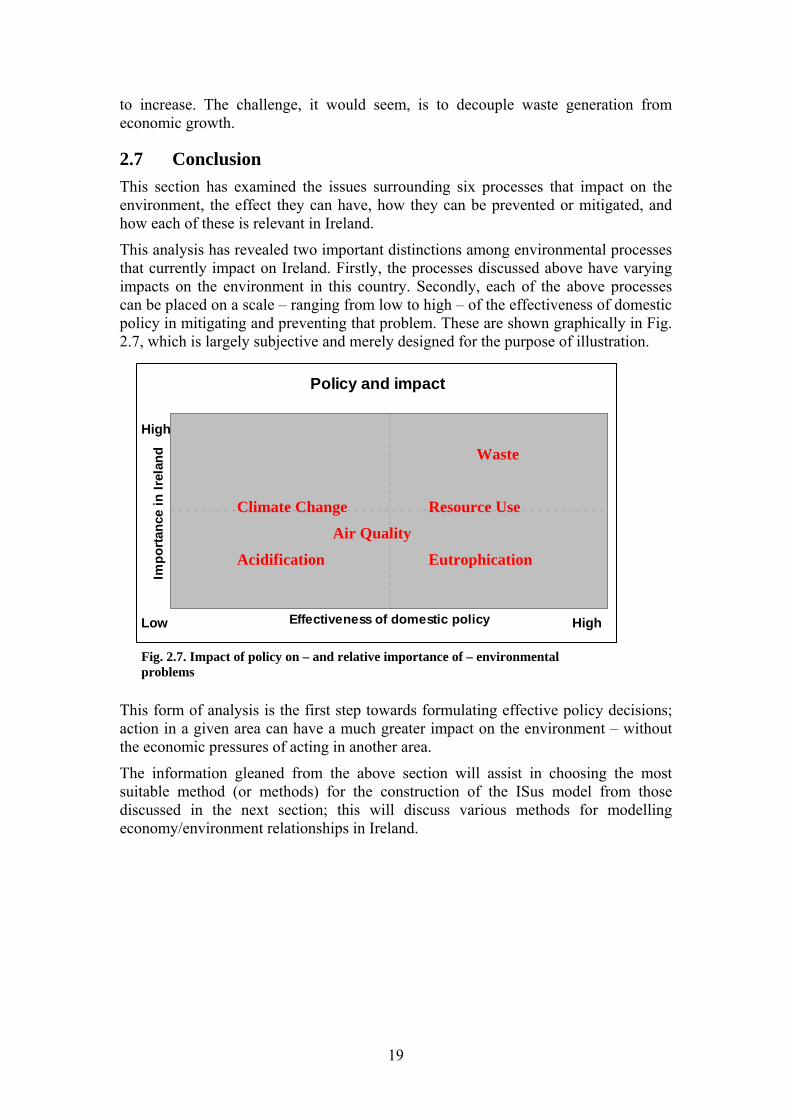
2.7 Conclusion This section has examined the issues surrounding six processes that impact on the environment, the effect they can have, how they can be prevented or mitigated, and how each of these is relevant in Ireland.

This analysis has revealed two important distinctions among environmental processes that currently impact on Ireland. Firstly, the processes discussed above have varying impacts on the environment in this country. Secondly, each of the above processes can be placed on a scale – ranging from low to high – of the effectiveness of domestic policy in mitigating and preventing that problem. These are shown graphically in Fig. 2.7, which is largely subjective and merely designed for the purpose of illustration.

Policy and impact

Effectiveness of domestic policy

Impo

rce

inan

dta

n Ir

el

High

Waste

Climate Change Resource Use

Air Quality

Acidification Eutrophication

Low High

Thacthe

Thsudisec

Fig. 2.7. Impact of policy on – and relative importance of – environmental problems

is form of analysis is the first step towards formulating effective policy decisions; tion in a given area can have a much greater impact on the environment – without economic pressures of acting in another area.

e information gleaned from the above section will assist in choosing the most itable method (or methods) for the construction of the ISus model from those cussed in the next section; this will discuss various methods for modelling

onomy/environment relationships in Ireland.

19

3. Modelling the environment

Little of the overall body of research in relation to environmental economic models focuses on Ireland.23 In analysing the body of literature in this area it is thus of little value to focus on those studies that are limited to this country.

As such, what follows is an analysis of environmental economic models, which are herein broadly grouped into seven categories: Input-output models, environmental Kuznets curve analyses, decomposition models, computable general equilibrium models, econometric models, optimisation models and a final category of ‘hybrid’ models, a relatively recent phenomenon that seeks a union between the social and physical sciences.

This section concludes with an analysis of land use models.

3.1 Emission models

3.1.1 Decomposition Index decomposition analysis requires the modeller to deduce the energy intensity of a given sector of the economy, and how this is determined by industrial production across the economy.24 Comparing this to a base year then allows the modeller to analyse any changes that have occurred in that sector, and over the economy as a whole. This methodology was popularised following the world oil crisis of 1973-74, as ‘energy researchers began to look for ways to quantify the impact of structural shifts in industrial production on total industrial energy demand in order to have a better understanding of the mechanisms of change in energy use in industry’ (Ang and Zhang, 2000, 1149; Greening et al., 1997; Ang, 1999). However, Ang notes that ‘more recently, with the growing concern about global warming and air pollution, a number of studies using the methodology to study energy-induced emissions of CO2 and other gases have been reported’ (1999, 1146-7).

In a review of literature on decomposition models in environmental and energy economics, Ang and Zhang recognise 124 studies over a twenty-two year period to

23 In Ireland, the relationship between greenhouse gas emissions and the economy has been modelled by Conniffe et al. (1997), Bergin et al. (2002) and Fitz Gerald (2004). Teagasc has modelled the impact of agriculture on greenhouse gas emissions (Behan and McQuinn, 2002). Work on the impact of economic activity on the generation of solid waste is described by Barrett and Lawlor (1995). The state of research on the link between economic activity on water use and emissions to water is described by Scott (see Scott et al., 2001 and Scott, 2004). Finally, a range of different types of research on transport has been carried out for Ireland (See, Department of Public Enterprise, 2000), and a simplified model of the transport sector is already incorporated into the ESRI’s HERMES model of the Irish economy. 24 Sectoral energy intensity is ‘a better measure of energy efficiency than the aggregate energy intensity, [and] is the amount of energy consumption that is required to yield a given level of output at the sectoral level’ (Ang and Zhang, 2000, 1149-50).

20

2000 (2000, 1150). It is interesting to note that only four of these include Ireland in their analyses.25

Two broad schools of decomposition methods are recognised by Ang (1999). These differ by the way in which the energy intensity from a given sector is compared to energy intensities in a base year.

1. The Laspeyres index method ‘follows the Laspeyres price and quantity indices in economics by isolating the impact of a variable through letting that specific variable change while holding the other variables at their respective base year values’ (Ang and Zhang, 2000, 1157). By comparing the production share of a particular industry at a particular time with its energy intensity and production share in a base year, the modeller can derive the estimated impact of structural change in the economy over the period. Similarly, by comparing the energy intensity of a particular industry at a particular time with its energy intensity and production share in a base year, the modeller can derive the sectoral intensity of that sector over the period, and see changes in this regard.

2. The Arithmetic mean Divisia index method is noted to be ‘more robust, exhibiting a smaller residual term with less variation’ (Greening, 2004, 4). The Divisia index compares the relative energy intensities of an industry to a base year in a multiplicative form such that a Divisia index of 1 would mean that the energy intensity in the year under analysis is the same as in the base year.

For mathematical descriptions of both the Laspeyres index method and the Arithmetic Mean Divisia index method see the appendix.

Greening et al. compare the two as follows:

‘The Laspeyres [method] compares each of the components of energy usage patterns with a fixed base year, while holding the other components constant. As a result, this index does not have the time or factor reversal properties of an ideal price index (see Fisher, 197226). The other main method previously used is the sample average Divisia method (Boyd et al., 1987, 1988; Torvanger, 1991). As opposed to the Laspeyres index, the Divisia index…does have the time reversal property but does not have the factor reversal property’ (1997, 376).

Ang notes some faults with both Laspeyres Index decomposition and Divisia index decomposition (1999, 1159-61). These are presented below:

1. Difficulties in selecting a method – It is often unclear which decomposition method is most appropriate for a given situation. Ang (1994) suggested three methods of selection: (a) whether or not the assumptions associated with the chosen method meet the study objective, (b) ease of use, and (c) magnitude of the residual.

2. Large residuals – Ang recognises that ‘when changes in the data between the decomposition years are drastic, the performance of the conventional and the adaptive weighting divisia methods can be shown to deteriorate and give a

25 These are Eichhammer and Mannsbart, 1997; Morovic et al., 1989; Morovic et al., 1987; and Sun and Malaska, 1998. 26 Fisher’s Ideal price index is the geometric mean of the Laspeyres and Paasche price indices.

21

large residual term. This situation can arise when decomposition is carried out using highly disaggregated data or on the aggregate intensity for a specific fuel’ (1999).

3. Zero values in the data set – The arithmetic mean Divisia index formulae have logarithmic terms (see equations (17) and (18) in the appendix). This could ‘lead to computational problems when zero values appear in the data set’ (Ang and Zhang, 2000, 1163).27

However, these problems have been overcome by the refined divisia index decomposition method, the details of which are introduced and explained in Ang and Choi (1997).

Finally, the accuracy of decomposition models can be improved by using either a rolling base year or an annually changing weighting system. Greening et al. explain that:

‘although computationally more intensive and requiring more data, time series methods capture more information about changes in the underlying effects over time or how energy consumption has evolved over time. These methods include the Adaptive Weighting Divisia (AWD) and the simple average Divisia method with a rolling base year. The AWD allows for changing weights or parameter values through time in response to changing energy inputs or outputs’ (ibid).

It is evident that the accuracy and applicability of decomposition models have improved over the last three decades. However, it is still uncertain which method might be most applicable in the case of Ireland. Further, the lack of prior research using this country in its analysis increases the risks associated with using a decomposition model to construct the Isus model, as there are few bases for comparison of any results the model might produce.

3.1.2 Environmental Kuznets Curve (EKC) analysis Stern explains that:

‘the environmental Kuznets curve (EKC) is a hypothesized relationship between various indicators of environmental degradation and income per capita. In the early stages of economic growth degradation and pollution increase, but beyond some level of income per capita, which will vary for different indicators, the trend reverses, so that at high income levels economic growth leads to environmental improvement. This implies that the environmental impact indicator is an inverted U-shaped function of income per capita.

27 Ang and Zhang observe that ‘in industrial energy demandata set] arises when a certain type of fuel begins or ceases1163).

22

Fig. 3.1. Typical shape of the Environmental Kuznets Curve

d analysis, the problem [of zero values in the to be used in an industrial sector’ (2000,

Typically, the logarithm of the indicator is modelled as a quadratic function of the logarithm of income…The EKC is named for Kuznets (1955) who hypothesized that income inequality first rises and then falls as economic development proceeds’ (2004, 1419).

The evidence for such a relationship is mixed, however. Harbaugh et al. (2001) and Stern (2004) are critical of the existing literature in support of a consistent relationship between environmental indicators and national wealth.

Although ostensibly an academic curiosity, EKC analysis has important policy implications. For instance, a developing nation with rising levels of pollution can justify potentially harmful policies on the grounds ‘that developing countries will automatically become cleaner as their economies grow’ (Harbaugh et al., 2001, 541).

Beckerman goes so far as to claim that ‘the best – and probably the only – way to attain a decent environment in most countries is to become rich’ (1992, 482). Stern finds fault with analyses such as Beckerman’s on two levels. Firstly, EKC analyses generally include assumptions in relation to constant returns to scale and consistency in technology and both the input and output mix of growing economies. Yet Stern notes that ‘though any actual change in the level of pollution must be a result of change in one of the proximate variables, those variables may be driven by changes in underlying variables that also vary over the course of economic development’ (2004, 1422).

Secondly, Stern conducts an econometric critique of EKC analysis, and notes the following criticisms:

• Heteroskedasticity – smaller residuals can be associated with countries with higher total GDP and population, although feasible generalised least squares (GLS) can be employed to resolve this problem.

• Omitted variables bias – Stern observes that in some cases the regressors that underlie a given relationship (between, say, pollution and GDP) may be correlated with variables that are omitted from the analysis. Further, he finds significant differences between the turning points for OECD and non-OECD countries. Finally, he concludes that serial correlation is present in these analyses.

• Cointegration – Stern finds that in some cases, though not all, the series that underlie EKC curves have stochastic trends (ibid, 1429).

However, despite the assessments of both Harbaugh et al. and Stern, the development of models similar to those provided by EKC analysis will be important in the construction of the ISus model. The dynamic relationship between economic growth and the ecological impact of the policies that encourage this growth will be an important consideration when modelling the effects of policy choices. Yet, one must be careful in so doing to avoid the pitfalls of previous EKC analyses.

3.1.3 Input-Output models According to its founder, Wassily Leontief,

‘input-output analysis describes and explains the level of input of each sector of a given national economy in terms of its relationships to the corresponding levels of activities in all the other sectors’ (1970, 262).

23

Essentially, this involves a matrix representation of the economy in order to predict the effect of changes in one industry on others, while at the same time modelling the effect of this interaction on consumers, the government and foreign suppliers.

The first effort to model the effect of these interactions on the environment was undertaken by Leontief himself, when in 1970 he sought to account for pollution and a new industry aggregation – the anti-pollution industry – within a hypothesised two-sector, two-good economy.

However, Van den Bergh and Hofkes note that ‘the most important recent study [in input-output environment modelling] is by Duchin and Lange (1994)’ (1999, 1114). Their ambitious model involves a detailed input-output model of the world economy, covering the dynamics of trade in sixteen regions and fifty sectors. This study sought to test the Brundtland Commission’s statement that growth and sustainable development could go hand in hand, and concluded that this is not the case.28

A common issue in relation to input-output models is that these models ‘are structurally fixed in the sense that sectoral classification and disaggregation, and assumed technologies, cannot change endogenously’ (van den Bergh and Hofkes, 1999, 1115).

One effort to overcome these problems is the Regional and Welsh Appraisal of Resource Productivity and Development (REWARD) project in the UK (see Ravetz, et al., 2003). The project distinguishes different regions of the UK and thus further subdivides the standard input-output modelling framework to create a Regional Economy-Environment Input-Output (REEIO) model. The REWARD project was designed with the specific intention of modelling policy options in the UK and as such may prove valuable as a comparative tool in constructing the Isus model.

Input-output models are generally considered to be a useful tool for short-term and static analyses. As a result, they can be less accurate than more dynamic methods in modelling over the medium- and long-term. Further, they focus on the production side of the economy and as such may be weak when modelling sectors such as households and international trade. However, the data and other information required to build an input-output model, as well as the ‘regionalisation’ that has been developed in a model such as REWARD, may prove useful in constructing the ISus model. As such, the development of an environmental input-output model has proven to be a useful first step this project.

3.1.4 Computable General Equilibrium (CGE) models Computable (or applied) general equilibrium models are the principal analytical tools of applied economic policy analysis. Conrad explains that ‘models of this type are a computer representation of a national economy or a region of national economies, each of which consists of consumers, producers and the government’ (1990, 1060), although these aggregations are further broken down as more powerful models simulate the economy with ever-greater accuracy.

28 Dellink et al. (1999) extend a computable general equilibrium (CGE) model to environment-economy relationships in the Netherlands up to 2030. Their principal conclusion – ‘that economic growth can be reconciled with a reduction in environmental pressure…[if] there is improved environmental efficiency combined with a significant restructuring of the economy’ (ibid, 153), counters that of Duchin and Lange. CGE models are discussed below.

24

Conrad notes that as ‘the practice of model-building itself has become increasingly systemised’ (1999, 1060) the variety of approaches in using these models to predict the effects of a chosen policy on the environment has grown, such that:

‘from a pragmatic point of view…[it has] become more and more difficult to understand why a carbon dioxide reduction target of 10 per cent calls for a CO2 tax rate of, for example, $20 by one model builder, but $300 by another’ (ibid).

In an investigation of eighteen distinct E3-CGE (energy-economy-environment computable general equilibrium) models that have been developed since 1998, Böhringer and Löschel (2006) investigate the coverage of both environmental and economic indicators in each of these models. They conclude that: ‘Operational versions of E3–CGE models have a good coverage of central economic indicators, whereas environmental indicators with complex natural science backgrounds and — in particular — social indicators are hardly represented’ (ibid, 61). In other words, CGE models are good at answering economic questions with regard to emissions and emission reduction for global and continental environmental problems. For local problems (e.g., urban air quality) or environmental problems that cannot be reduced to emissions (e.g., biodiversity), CGE models are less appropriate. Similarly, CGE models are not suitable for analysing the social dimension of sustainable development.

Perhaps the most prominent developments in CGE modelling of the environment have been the calculations of a sustainable national income (SNI) for The Netherlands.

SNI is a concept that was popularised by Hueting in the 1970s. Verbruggen et al. explain that:

‘According to Hueting, the objective to construct a SNI boils down to a correction of national income for environmental losses. With environmental losses is meant the foregone use of the environment due to competition between the different functions the environment performs to sustain economic activities and human life. As national income is recorded in market prices, the correction for environmental losses should be in comparable terms. Hence, ideally, shadow prices have to be found on the basis of demand and supply curves for environmental functions. Then, environmental losses can be expressed in market prices and deducted from national income to arrive at SNI’ (2001, 276).

Hueting makes a number of assumptions when defining SNI, among them that shares of imports and exports are constant (as opposed to an assumption of constant relative prices on the world market) and that the final figure for SNI is expressed in new equilibrium prices (as opposed to relative prices of a given base situation). However, Verbruggen et al. broaden this analysis. Because ‘no decisive preference can be given to one of the two assumptions on foreign trade as well as on the use of old or equilibrium prices, four SNI variants are calculated’ (ibid, 284). These are shown in Table 3.1 along with the calculated impact of implementing SNI under each set of assumptions.

25

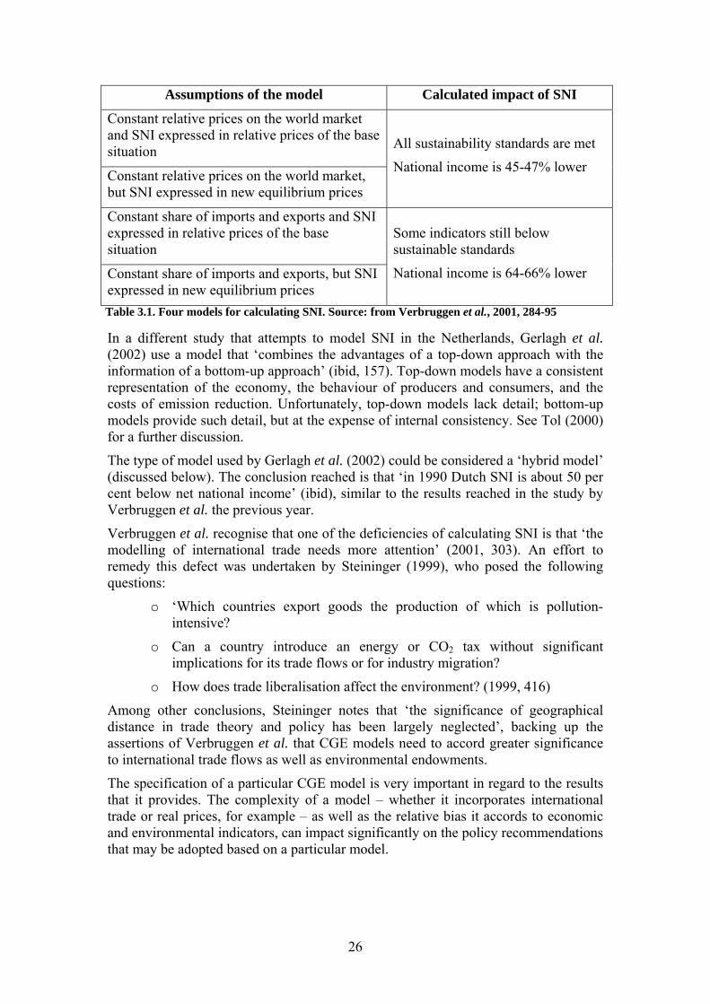
Assumptions of the model Calculated impact of SNI

Constant relative prices on the world market and SNI expressed in relative prices of the base situation

Constant relative prices on the world market, but SNI expressed in new equilibrium prices

All sustainability standards are met

National income is 45-47% lower

Constant share of imports and exports and SNI expressed in relative prices of the base situation

Constant share of imports and exports, but SNI expressed in new equilibrium prices

Some indicators still below sustainable standards

National income is 64-66% lower

Table 3.1. Four models for calculating SNI. Source: from Verbruggen et al., 2001, 284-95

In a different study that attempts to model SNI in the Netherlands, Gerlagh et al. (2002) use a model that ‘combines the advantages of a top-down approach with the information of a bottom-up approach’ (ibid, 157). Top-down models have a consistent representation of the economy, the behaviour of producers and consumers, and the costs of emission reduction. Unfortunately, top-down models lack detail; bottom-up models provide such detail, but at the expense of internal consistency. See Tol (2000) for a further discussion.

The type of model used by Gerlagh et al. (2002) could be considered a ‘hybrid model’ (discussed below). The conclusion reached is that ‘in 1990 Dutch SNI is about 50 per cent below net national income’ (ibid), similar to the results reached in the study by Verbruggen et al. the previous year.

Verbruggen et al. recognise that one of the deficiencies of calculating SNI is that ‘the modelling of international trade needs more attention’ (2001, 303). An effort to remedy this defect was undertaken by Steininger (1999), who posed the following questions:

o ‘Which countries export goods the production of which is pollution-intensive?

o Can a country introduce an energy or CO2 tax without significant implications for its trade flows or for industry migration?

o How does trade liberalisation affect the environment? (1999, 416)

Among other conclusions, Steininger notes that ‘the significance of geographical distance in trade theory and policy has been largely neglected’, backing up the assertions of Verbruggen et al. that CGE models need to accord greater significance to international trade flows as well as environmental endowments.

The specification of a particular CGE model is very important in regard to the results that it provides. The complexity of a model – whether it incorporates international trade or real prices, for example – as well as the relative bias it accords to economic and environmental indicators, can impact significantly on the policy recommendations that may be adopted based on a particular model.

26

3.1.5 Econometric models By its nature, an econometric model is an economic model formulated so that its parameters can be estimated if one makes the assumption that the model is correct. As such, formulating an econometric model of the environment requires some degree of prior knowledge about the likely inputs and outputs that affect both the environment and economy of a chosen system. Therefore, models of this kind are often actually hybrid models that seek firstly to estimate the likely parameters of the environment-economy relationship, and secondly to test the nature of that relationship by using econometric methods.

For example, although E3ME (short for Energy-Environment-Economy Model of Europe) – a pan-European environmental modelling project using econometrics – claims to ‘provide a one-model approach in which the detailed industry analysis is consistent with the macro analysis’, in reality it ‘combines the features of an annual short- and medium-term sectoral model estimated by formal econometric methods with the detail and some of the methods of the CGE models’ (Cambridge Econometrics, 2006). Nevertheless, the E3ME model is capable of being recalibrated to produce predictions and policy alternatives (Barker, 2000).

Don (2004) has noted that in the absence of a hybrid model ‘the interaction between the policy-maker and the model-cum-expert system then takes the form of an iterative trial-and-error procedure’ (25). Far from being a fault in econometric modelling of policy choices, this procedure can help to simulate the estimation of parameters – such as a welfare function – that would otherwise be arrived at by a system of ‘prior knowledge’ that may or may not involve another form of model (ibid).

In an Irish context, there are currently two significant models of the economy – the Central Bank’s model and the ESRI’s HERMES model.29

The Central Bank’s model has been in existence since 1999, and has recently been updated and recalibrated (see McQuinn et al., 2005). Although it can be used as a ‘stand-alone’ model, it has also been included in ‘linked mode simulations with other country models to generate euro area projections and responses to shocks’ (ibid, 3). In a domestic context, the model is regularly used to model medium- and long-term forecasts of the national economy, and has been used to test the economy’s readiness for ‘shocks’ such as oil price increases and a correction in the construction sector (ibid).

The ESRI’s medium-term economic model was developed in similar circumstances, as part of a Europe-wide effort to coordinate national macroeconomic modelling under a project entitled HERMES in the early 1980s. Of the national models developed at this time, the Irish model is one of the few that is still in existence30, and

29 Other much smaller models are available as part of the EU QUEST project, and the UK NIESR NiGEM model. In the past, general equilibrium models have been developed by University College Dublin and Trinity College, Dublin, but they have not been developed or maintained on a continuous basis. 30 Bossier et al. (2000 and 2002) have used the Belgian version of the HERMES econometric model – in conjunction with an input-output model – to model CO2 emissions in Belgium. In other countries, pure econometric models have been replaced with models that are a hybrid between econometric models and computable general equilibrium models. See Bray et al. (1995) for a review of the situation in the UK.

27

has developed and evolved during the last twenty years. The model is structured as follows:

‘The ESRI economic model of the Irish economy focuses initially on the output (or production) relationships [between actors in the economy], and examines the downstream expenditure and income consequences. The key mechanisms within the model are:

1. The exposed sector is driven by world demand, elements of domestic demand, and cost competitiveness.

2. The sheltered market sector (services and building) is driven by domestic demand.

3. The public sector is policy-driven, with treatment of borrowing and debt accumulation

4. Wages are determined in a bargaining model, and influenced by the factors that affect the supply and demand for labour – e.g. prices, taxes and unemployment.

5. The labour market is open and influenced by conditions in the UK labour market.’ (Bergin et al., 2003)

Macro-econometric models are particularly useful in the medium term. For short-term forecasting, other model types (particularly decomposition and input-output models) can be more accurate.

It is thus perhaps not surprising that in order to analyse the economic impacts of the 1997 EU energy tax in the short-, medium- and long-term, Jansen and Klaassen (2000) employed three different types of models. As the authors explain:

‘Three different macroeconomic models were employed to assess the economic impacts of the directive: HERMES (Harmonised European Research for Macrosectoral and Energy Systems), GEM-E3 (General Equilibrium Model for Economy-Energy- Environment), and E3ME (Energy-Environment-Economy Model for Europe). While having a number of points in common, these models cover a broad scope of economic modelling approaches, thus allowing insights into the robustness of the models involved’ (ibid, 183).

As such, the authors employ input-output, Computable General Equilibrium and econometric models in the same framework.

In constructing the ISus model it may be advisable to build on existing models such as those discussed in this section, as forecasts are required for the medium- and long-term, but not necessarily for the short-term.

3.1.6 Optimisation models Optimisation models consist of an intertemporal objective that must be optimised subject to a set of constraints (on time, money, resources, etc.).

Feenstra et al. explain that:

‘optimal control theory originated as a mathematical tool to solve problems of dynamic optimisation. Applying it to economic problems allows the explicit consideration of time. This makes it suitable for

28

analysing the intertemporal trade-off between current consumption and future pollution or exhaustion of natural resources that is inherent in many environmental problems’ (1999, 1099).

The Dynamic Integrated Climate-Economy (DICE) model of the economics of global warming presents just such a situation. Nordhaus explains that it was developed to provide input to the Intergovernmental Panel on Climate Change (IPCC), the World Climate Conferences and the United Nations Conference on Environment and Development (the Earth Summit).

One difficulty that Nordhaus recognised was that the DICE model ‘must take into account, above all, the long time lags between actions or policies and responses. Nations must take steps now in order to slow climate change over the coming centuries’ (1992, 4). The DICE model adopted the following format:

‘The basic approach is to use the Ramsey growth model31 of optimal economic growth with certain adjustments and to calculate the optimal path for both capital accumulation and GHG-emission reductions. The resulting trajectory can be interpreted as either the most efficient path for slowing climate change given initial endowments or as the competitive equilibrium among market economies where the externalities are internalised using the appropriate social shadow prices for GHGs’ (ibid).

By 2000, Nordhaus and Boyer had updated the DICE model and the closely related RICE – the Regional Integrated model of Climate and the Economy. They note that ‘the purpose [of the updated RICE model] is to integrate scientific knowledge of the dynamics of climate change with understanding of the economic aspects of emissions of greenhouse gases and damages from climate change’ (2000). As such, it could be classified as a hybrid model (see below), as it encompasses elements of natural science modelling in order to derive a more accurate estimation of climate change. That it derives from DICE, and that its results are used as a basis of comparison for this model (and vice-versa), means that it is more prudent to discuss it here. Indeed, its economic basis is from optimisation modelling; as the model’s designers note: ‘the basic approach taken in analysing the economics of climate change is to consider the trade-off between consumption today and consumption in the future’ (ibid).

The RICE model has unearthed three ‘major results’:

• Firstly, Nordhaus and Boyer note that an emissions growth path ‘that limits CO2 concentrations to no more than doubling of pre-industrial levels is close to the “optimal” or efficient policy’. By contrast, current approaches, such as the Kyoto Protocol, are highly inefficient, with abatement costs approximately ten times their benefit in reduced damages’ (ibid).

• Secondly, according to the RICE model, ‘the optimal carbon price in the near term is in the $5 to $10 per ton range’ (ibid).32

31 The Ramsey growth model is a neo-classical model of economic growth. Unlike the Solow model, the Ramsey growth model, does not incorporate an endogenous saving rate. As a result, the saving rate in general is not constant and the convergence of the economy to its steady state is not uniform. 32 On Jan 2, 2007, the price was €6.55/tCO2 according to www.pointcarbon.com

29

• Thirdly, the RICE model is far less pessimistic about future trends in climate change than previous and subsequent models have been. It predicts a baseline scenario of uncontrolled warming of 2°C by 2100, compared to ‘at least a 50% risk of exceeding 5°C global average temperature change’ predicted in the Stern Review on the economics of climate change (2006, iv), and the 3.3°C predicted in the original DICE model (Nordhaus and Boyer, 1999).

Fankhauser and Tol (2005) present another example of optimisation models in environmental economics. They employ the basic tenets of the DICE model, allowing for a focus on changes in ‘dynamic interlinkages’ (how climate change may affect welfare in the future), capital accumulation and savings behaviour as climate change affects the economy and vice versa. Their analysis concludes that ‘climate change will always have a negative effect on the capital stock…[and] net savings will always be reduced. These results hold independent of the choice of discount rate’ (ibid, 12). This result is significant because, as the authors explain, ‘the traditional enumerative studies [econometric, decomposition, input-output models] of climate change impacts underestimate the true costs of climate change’ (ibid).

However, Fankhauser and Tol are also keen to point out two limitations of optimisation models. Firstly, in their own model and others, savings and capital accumulation are not the only ways in which climate change can affect economic growth, although their model could be expanded to account for more parameters, as well as international trade effects (the model assumes a closed economy). Secondly, they note some theoretical problems with their model. They have largely ignored the interaction between a changing environment and health effects, and have assumed that welfare maximisation is the rational choice for society (2005, 13).

Finally, in another example of a hybrid model of environment-economy relationships, Klaassen et al. (1999) link the MARKAL optimisation model33 with an input-output model. The authors explain that:

‘The linkage between MARKAL and the IO model is established through two interfaces. The first interface transforms and re-allocates energy costs associated with MARKAL technologies to comply with the structure of the IO model. The second interface uses the results from the model to calculate the induced changes in useful energy demand level for MARKAL. This procedure is iteratively repeated until the model results of MARKAL and IO converge and a new optimal solution is found’(ibid, 1).

Another extension of optimisation modelling has been undertaken by the International Institute for Applied Systems Analysis (IIASA). The MESSAGE model is ‘a systems engineering optimization model used for medium- to long-term energy system planning, energy policy analysis, and scenario development’ (IIASA, 2006). MESSAGE provides the framework for analysing energy systems from resource extraction to usage across eleven world regions. It has been used to assess mitigation strategies for carbon dioxide (Riahi and Roehrl, 2000a) and other greenhouse gases (Riahi and Roehrl, 2000b), as well as for deriving scenario analyses for the

33 MARKAL (MARKet ALlocation) ‘is a generic model tailored by the input data to represent the evolution over a period of usually 40 to 50 years of a specific energy system at the national, regional, state or province, or community level’ (IEA, 2006).

30

Intergovernmental Panel on Climate Change (IPCC) (Nakicenovic, 2000). The model is constantly extended, and is now the first to include emissions of black and organic carbon their abatement (Rao, personal communication, 2006).

IIASA has also developed the Regional Air Pollution Information and Simulation (RAINS) model, and its extension, the Greenhouse Gas and Air Pollution Interactions and Synergies (GAINS) model. Both of these are optimisation models, but whereas RAINS addresses threats to human health and the environment that are posed by acidification, GAINS uses scientific methods to analyse the synergies that occur between various pollutants in the atmosphere, and – separately or jointly – how they cause a variety of environmental effects at the local, regional and global levels. The models’ designers explain that ‘The RAINS model framework makes it possible to estimate, for a given energy and agricultural scenario, the costs and environmental effects of user-specified emission control policies’ (Amann et al., 2004). As such, it qualifies as an optimization model.

Optimization models have also been applied to find least-cost solutions to meeting targets for eutrophication, for the Rhine basin (van der Veeren and Tol, 2001), for the Baltic sea catchment (Gren et al., 1997), and even for the whole of Europe (Warren and ApSimon, 2000). The last study appropriately includes the interactions between acidification and eutrophication policies.

It is apparent that optimisation models are widely used in environmental economic modelling. However, the experience and research of Bray et al. advocates a careful approach to the use of such models that requires the ongoing participation of the eventual policy maker.

3.1.7 Hybrid models Tol explains that:

‘Hybrid models are economic models with a detailed representation of the supply side of energy, including transformation technologies and reserves of energy carriers. Prime examples are MERGE, CETA, SGM, GTEM, and MS-MRT. Unlike top down models, which rely on aggregate production functions, hybrid models cannot burn more gas than there is, distinguish between nuclear power and biomass as alternatives to fossil fuels, and explicitly treat the changes in relative prices between alternative energy carriers. Hybrid models are thus considerably more realistic and offer substantially more insight than traditional top-down models. Hybrid models also have better economics than bottom-up models’ (2000, 3).

MERGE and CETA are optimization models, resembling DICE and RICE in principle but with much detail added. SGM, GTEM and MS-MRT are computableselected production functions were replaced w

31

Fig. 3.2. Overview of the MERGE model. Source:Manne et al. (1995, 18)

general equilibrium models, but ith engineering detail.

Each of the models identified by Tol is discussed below.

• MERGE (Model for Evaluating Regional and Global Effects of GHG reductions) ‘consists of a series of linked modules representing the major processes of interest’ (Manne et al., 1995, 18). These modules represent the cost of reducing emissions, the reactions of natural systems to these emissions, and the reaction of human and natural systems to changes in the atmospheric/climate system (ibid). This is achieved by integrating three submodels: Global 2200 (an applied general equilibrium model for assessing the costs of emissions out to the year 2200), a climate submodel (which models ‘the relationship between man-made emissions and atmospheric concentrations and the resulting impact on temperature’), and a damage assessment submodel (that values the environmental impact of climate changes) (Manne and Richels, 1999, 4).

• The CETA (Carbon Emissions Trajectory Assessment) model is structurally based on the Global 2100 model (the fore-runner to the Global 2200 model that forms the basis of MERGE – see above), but incorporates an energy submodel, a production submodel and a warming submodel (Peck and Teisberg, 1992). As such, it is quite similar to the MERGE model (Peck and Teisberg, 1999, 368).

Fig. 3.3. Overview of the CETA model. Source: Peckand Teisberg, 1992, 58

• SGM (Second Generation Model) builds on the GCAM (Global Change Assessment Model), a model developed in the US in the early 1990s. It is ‘a computable general equilibrium model that projects economic activity, energy consumption, and carbon emissions for twelve world regions’ (MacCracken et al., 1999, 27). The model is outlined in Fig. 3.4. Edmonds et al. explain the diagram:

‘On the left hand side of Fig. 3.4 are two sectors that create final demands for new net goods and services production in the economy, the household and government sectors. On the right hand side of Fig. 3.4 are the sectors of the economy that produce new final goods and services, the energy production and transformation, agricultural, transportation, and industrial and services sectors. In addition to the production and consumption of goods and services, Fig. 3.4 indicates that the release of greenhouse related emissions to the atmosphere are

32

Fig. 3.4. Overview of the SGM model. Source: Edmonds et al., 2004, 10

tracked by the point of release’ (Edmonds et al., 2004, 9-10).

• GTEM (Global Trade and Environment Model) is a recursive dynamic general equilibrium model of the world economy developed by the Australian Bureau of Agricultural and Resources Economics ‘specifically to address policy issues with long term global dimensions’ (Pant, 2002). The regional coverage includes detail for only 5 EU countries: Denmark, Finland, Germany, Sweden, and the United Kingdom. The greenhouse gas coverage in GTEM includes carbon dioxide, methane and nitrous oxide, as well as removals by forest sinks. Viguier et al. note that ‘the GTEM model has been used to analyze the economic impacts of the Kyoto Protocol on different regions, such as developing countries and European countries’ (2003, 464; and see Tulpulé et al., 1999).

• The MS-MRT (Multi-Sector Multi-Region Trade) model adopts a similarly disaggregated depiction of the world economy as is portrayed in the MERGE model. According to the consultancy CRAI, MS-MRT is capable of analysing ‘differences in energy intensities across countries and differences in the composition of industries’ as it ‘includes Social Accounting Matrices and bilateral trade flows for 55 countries/regions and 8 industries’ (CRAI, 2006). Otherwise, it is similarly structured to MERGE, such that it adopts its ‘business as usual’ scenario from that model, while allowing policy changes and

33

changes in production, trade and technology/productivity to be modelled in MS-MRT.

The hybrid models above are extended economic models. Tol (2000) also recognises another form of hybrid models: extended engineering models. In explaining these he notes that:

‘The novel aspect is that these models, like new growth models34, endogenise technological progress based, unlike new growth models, on learning by doing, implying that the average costs fall if volume increases, not because of economies of scale, but because of experience gained’ (ibid, 4).

As Tol notes, it is possible for these models to better describe the economy (than earlier engineering models might), but their assumptions and parameterisations may undermine any result.

A project was launched in 2002 by the Alliance for Global Sustainability involving two separate research groups35 to assess the role of technological change in transportation systems, and their environmental impact (see Krzyzanowski et al., 2004). The authors explain that:

‘While the first group [MIT] was concerned with linking the general-equilibrium top-down and the bottom-up, energy-systems (MARKAL) approach, the focus of the second group was the integration of technological learning by doing (LBD) in transportation technologies in the “bottom-up” component of the modelling system. MIT has successfully completed the link between the three models (without endogenous technological learning components) in a consistent framework (Schafer and Jacoby, 2003), while PSI [the Paul Scherrer Institute] has contributed to the introduction of LBD in the context of the MARKAL model and of a stand-alone simplified transportation model’ (ibid).

Essentially, hybrid models of this kind look outside the traditional disciplines of the social sciences and engage the natural sciences, particularly models associated with engineering systems. As such, they can have a better understanding of technological change and how it can impact on the environment.

The word ‘hybrid’ can thus describe two types of environmental economic model; one with a detailed representation of energy supply; or one that builds on new growth models, but with a more complex description of technological change. Whereas the latter is a developing area of research that has only recently been applied to environmental modelling, the former is something of a necessity in building advanced – particularly econometric – models.

34 New growth models (or ‘endogenous growth models’) are distinguished by their treatment of technological development. They rely on ‘virtuous cycles’, wherein new technologies are ‘produced’ and importance is thus given to human capital. Some of the knowledge associated with the innovation “spills over” to other economic actors, which increases those actors’ ability to innovate. 35 The two research groups are the Center for Technology, Policy & Industrial Development, Massachusetts Institute of Technology (MIT) (H. Jacobi and A. Schäfer) and the Energy Economics Group of the Paul Scherrer Institute (PSI) in Switzerland (S. Kypreos, L. Gutzwiller, D.A. Krzyzanowski and L. Barreto).

34

3.2 Land Use Models

3.2.1 Land use in economics The root of the word economics is in the Greek for ‘laws of the household’ – particularly referring to the traditional farm, for which subsistence and barter were more important than trade.36 The first systematic economists, the Physiocrats, argued that agriculture was the primary sector, and that land was the only true source of value. The Classical economists similarly placed substantial emphasis on agriculture and land. David Ricardo’s (1815) notion that land rents reflect land quality is hotly debated today (Mendelsohn et al., 1994; Darwin, 1999; Schlenker et al., 2005, Timmins, 2006). Economic textbooks still explain decreasing returns to scale with the example of additional farmhands on a field using Turgot’s (1793) intensive margin.37 Steuart’s (1767) extensive margin,38 another source of decreasing returns to scale, similarly seeks to explain land use patterns. Further, externalities are often introduced with the example of the beekeeper and the farmer.39 However, as agriculture is a minor economic sector in industrialized countries nowadays, it is the vertically integrated manufacturing sector that serves as the canvas upon which much of modern economic theory is painted.40

Land use has attracted even less attention. In the Classical literature, there is Von Thuenen’s (1826) model of farm specialization as a function of the distance to town, and Zipf’s Law on the relative size of cities (e.g., Duranton, 2006).41 In economic geography, there are the location analysis of Weber (1909) and the central-place theory of Christaller (1966) and Loesch (1964). But land use plays a minimal role in current economic theory. Partly, this may be because land is a minor problem. The built environment, and hence more than 95% of the world economy, occupies less than 1% of the land surface (Gruebler, 1994). Distance matters, of course, but can be parameterized (e.g., as in Samuelson’s iceberg model42) without an explicit two-dimensional model of the land surface. Krugman (1998b) offers another explanation: City formation can only be explained by a combination of congestion and agglomeration externalities. As agglomeration implies increasing returns to scale, city formation resisted rigorous analysis until the monopolistic competition revolution (Dixit and Stiglitz, 1977).

This has now changed (Krugman, 1991; Fujita et al., 1999; Brakman et al., 2001). New economic geography offers micro-founded, general equilibrium models of activity location (Krugman, 1998a). See Martin (1999) and Henderson (1974) for a defence of the “old” economic geography of Isard (1956). New international economics has its roots in the monopolistic revolution too. Rossi-Hansberg (2005) shows that, in a spatial model, tariffs and transport costs are different – tariffs are step

36 The word “economics” is from the Greek words οικος [oikos], meaning “family, household, estate,” and νοµος [nomos], “custom, or law”. 37 Intensive margin refers to the degree (intensity) to which a factor of production is utilized or applied. 38 Extensive margin refers to the range to which a factor of production is utilized or applied. 39 Meade (1952) described how an apiary next to an orchard causes a positive externality. For a summary, see Maskin (1994, 333-4). 40 See Hubacek and van der Bergh (2006) for more historical perspective. 41 Zipf (1935) specified the functional form, but only applied it to the relative frequency of words. 42 Samuelson (1954) described how a moving iceberg loses mass as it drifts. This is analogous to goods being lost in transport, which can be difficult to model.

35

changes, whereas transport costs are continuous. Bioeconomics is also adopting spatial analyses (Sanchirico and Wilen, 1999), particularly in the investigation of marine protected areas (Smith and Wilen, 2003). General equilibrium models of ecosystems are now emerging (Tschirhart, 2000, Finnoff and Tschirhart, 2003) and have recently been extended to include land – as a factor of production, not for humans but for plants (Eichner and Pethig, 2006). As promising and exciting as these developments may be, this is theory only (Neary, 2001) – with a few empirical tests (see Brakman et al., 2006). Although this work is increasingly applied (e.g., Stelder, 2005), practical applications cannot be expected in the near future – at least, not in the sense of a calibrated global model that can be used for numerical questions on climate policy. Empirical analysis and operational models particularly suffer from lack of data. Nordhaus (2006) is a first step towards spatially explicit economic data.

Recent developments in land use modelling have hardly been revolutionary, applying established methods, and relying instead on a break-through on the data front in order to be distinguished. Only now do we have access to globally consistent databases of land use, coupled with data on the physical characteristics of land and the environment.

3.2.2 Geographic models of land use Geographers obviously have a keen interest in land use. Most geographic models are small-scale, often limited to a small part of a country, and cannot be generalized; indeed, many geographers resist generalization and large-scale research, and mathematical analysis and numerical models are not core tools for much of this work. Nonetheless, there are a few large-scale models of land use. Heistermann et al. (2006) distinguish between statistical models and rule-based models.

CLUE is a prominent example of a statistical model (Veldkamp and Fresco, 1996). Most of the equations in the model are estimated by multiple regression, but the model is completed by rule-based competition and transition. The largest scale applications of CLUE are for China (Verburg et al., 1999) and for tropical South America (Wassenaar et al., forthcoming). The latter model works at the impressive resolution of 3x3 km.

SALU and IMAGE are examples of rule-based models. In both of these models demand-driven expansion of agricultural production is met on the basis of a suitability ranking, based on soil, climate, distance and so on. The trade-off between infra- and extra-marginal expansion is modelled in a similar way. The SALU model (Stephenne and Lambin, 2001, 2004) is restricted to the Sahel, but the IMAGE model (Alcamo et al., 1998) is global with a spatial resolution of 0.5ºx0.5º.

In ACCELERATES (Rounsevell et al., 2003) and KLUM (Ronneberger et al., 2005), the rules are derived from profit maximization. In both cases, a risk-averse farmer maximizes profits given prices of inputs and outputs, and a probability distribution of yields.

3.2.3 Economic models of land use Partial equilibrium models are based on the same optimization principles as KLUM, but include the response of prices to changes in production and consumption. Examples are IMPACT (Rosegrant et al., 2002) and WATSIM (Kuhn, 2003) for agriculture; GTM (Sohngen et al., 1999) for forestry; and AgLU (Sands and Leimbach, 2003) and FASOM (McCarl, 2004; Adams et al., 2005) for both

36

agriculture and forestry. The distinct advantage of partial equilibrium models is that they are more flexible and less computationally intensive than general equilibrium models. Further, their data needs are less at any given level of spatial and sectoral resolution. As a result, partial equilibrium models often have substantial spatial and crop detail.

The disadvantage of partial equilibrium models is that the rest of the economy is ignored. General equilibrium models do not have this problem. The first global computable general equilibrium model with land use disaggregated by physical characteristics is the FARM model by Darwin et al. (1995). Land, a non-tradable endowment in a CGE model (perhaps as part of an aggregate endowment), is split into a number of different categories, distinguished by productivity. Land endowment by category is an aggregate taken from a spatially explicit bioclimatic model. The model has been used to estimate the impacts of climate change (Darwin, 1999, 2004; Darwin and Kennedy, 2000), of sea level rise (Darwin and Tol, 2001), and of nature conservation (Lewandrowski et al., 1999) – each of which changes the relative land endowments.

Note that changes in demand for land were met, in the spatially-explicit biophysical model, on the basis of rules, rather than on the basis of optimal behaviour. That is, Darwin et al. (1995) brought biophysical realism into their economic model, but they did not bring economic realism into their biophysical model.

GTAP-L (Burniaux and Truong, 2002) extends the work of Darwin et al. (1995) through the introduction of the transformation of land (from one crop to another), thus introducing competition between alternative land uses. The input data were imperfect, however. The GTAP-AEZ model (Hertel et al., 2006) combines the theoretical and empirical strengths of FARM and GTAP-L.

3.3 Conclusion A number of modelling methods have been discussed in the above section. It is likely that in the construction of the ISus model many of these methods will have to be employed, particularly in relation to the construction of ‘sub-models’ (see section 6, below). For example, the prototype ISus model developed by O’Doherty and Tol (2007) took the form of an environmental input-output model, while in its final incarnation the model will link with the ESRI’s HERMES model – an econometric model of the Irish economy. Land use models are likely to be important also.

All of the models noted above rely to some degree on price information and valuation of the environment. As such, this will be discussed in the next section.

37

4 Environmental valuation

Recreational resources such as forest parks, river activities or hiking are often the victims of commercial, agricultural or residential development. These environmental amenities are open to public use and can often be appreciated at no cost. However, the preservation of these sites from development depends on their perceived value. The absence of a market for these goods does not imply that they have no value. Indeed, as they impart a social benefit on their users (through recreation) a monetary value can be attributed to them – and this monetary value can be used to demonstrate the worth of nature conservation. The values of environmental amenities can be divided into two main groups ⎯ use values and non-use values.

Use values are those that are derived from an individual’s direct enjoyment of the environment. For a fisherman, the use value of a fully stocked river is very high. On the other hand, non-use values do not require that any utility be derived from the use of the resource. The utility an individual gains from the environmental good is intrinsic. For instance, for someone living in Ireland, the use value of an elephant in Zambia is minimal. Nevertheless, individuals still associate the possibility of being able to someday potentially see that elephant with a value ⎯ an option value. Individuals can also improve their utility just by knowing that elephant exists, this is the existence value of an environmental amenity or that their children may one day benefit from its existence, this is the bequest value.

The sum of these values is the Total Economic Value (TEV). The development of techniques that allow economists to calculate these values has been relatively recent and these methods are still being improved, although not all take into account use and non-use values. Nevertheless taking into account the TEV of an environmental amenity when addressing environmental policy is crucial. The following techniques are those most commonly used in practice.

3.4 Valuation theory Valuation methods are commonly divided into revealed preference and stated preference techniques. Revealed preference techniques derive the value of environmental amenities from market prices, while stated preference techniques ask individuals directly how much they value a specific quality level of an environmental amenity. While certain techniques are more applicable to certain types of environmental resources than others, all results from these projects should be taken purely as orders of magnitude and guidelines. Revealed preference methods are largely limited to use values, while stated preference methods can estimate both use and non-use values; revealed preference methods are more reliable, however, and less subject to bias.

4.2.1 Hedonic pricing The hedonic pricing method is a revealed preference technique. This is a regression method that links the prices of goods such as property values or wages (whose separate characteristics can be analysed) to environmental attributes. By decomposing a market good into separate characteristics, these can then be used to estimate how much the price varies in relation to each of the characteristics. First, Willingness-To-

38

Pay (WTP) for a good with certain attributes is estimated, then the demand function for a change in an environmental amenity is formulated and the associated consumer surplus can be estimated. Individual consumer surpluses are then aggregated to obtain the total value of a change in the environmental amenity. The hedonic pricing technique can be difficult to implement in practice due to the amount of variables and data required for it to be feasible. Moreover, it does not take into account non-use values or households’ future expectations, both of which are further limitations of the hedonic pricing technique.

4.1.2 The Travel Cost Method The travel cost method (TCM) is another revealed preference method of estimation. The costs incurred by a person when visiting a site, such as entry fees, accommodation costs and the time and nuisance costs of travel, can be used to infer the value attributed by that person to a visit. The value of the site can be derived from the demand function estimated by observing users’ behaviour in relation to costs sustained per number of visits. Degradation or amelioration in site quality can then be valued in monetary terms. There are two types of TCM, the Zonal Travel Cost Method (ZTCM) and the Individual Travel Cost Method (ITCM). The former takes into account the frequency rate for different zones, while the latter examines the behaviour of a single user.

Although the method is frequently used, there are a number of problems. First, as surveys are usually conducted on site there can be a sample bias, as non-visitors are not taken into account. Secondly, the likelihood of a person being sampled will depend on how often that person visits the site; this is the problem of endogenous stratification. Moreover, the technique does not take into account the fact that trips may be multi-purpose and that different sites, although they comprise the same amenity, can be quite distinct.

4.1.3 Contingent valuation techniques Contingent valuation methods are a type of stated preference technique, which can assess use and non-use values. Individuals are asked directly how much they would be willing-to-pay for an increase in the quality of an environmental amenity or how much they would be willing-to-accept in compensation for a decrease in the quality of an environmental good. From these questions it is possible to infer the willingness-to-pay (WTP) or willingness-to-accept (WTA) for a unit change in the quality of an environmental amenity and consequently construct a hypothetical market for that amenity and put a monetary value on the good. In practice, this is achieved by asking individuals a series of questions. They can be in an open-ended referendum format, i.e. of the type “how much would you be willing-to-pay to conserve this area of forest?” There are also dichotomous questions such as “would you be willing-to-pay €5 for an increase in the quality of this good?” Finally, questions can form part of an iterative bidding process, e.g. “Would you be willing-to-pay €10? If yes, then would you be willing-to-pay €15? If no, then would you be willing-to-pay €5?”, etc.

As with any of these techniques there are problems relating to data collection and the model. First, it has been argued that results can vary a great deal depending on the type of question asked. Moreover, it would seem that respondents have difficulty conceptualising an inexistent market (hypothetical market bias) and may overstate their WTP or may answer strategically instead of truthfully. Finally, results can be biased, as some respondents will have a tendency to free-ride. In order to avoid these

39

problems, the payment vehicle and amount will have to be made clear to respondents before they reply to questions.

4.1.4 Choice modelling Choice modelling comprises choice experiments, contingent ranking and contingent rating, which are all stated preference methods. Respondents are given a choice of scenarios which comprise different characteristics at different levels and are asked, depending on the method, to respectively choose their most preferred scenario, to rank them from their most to least preferred, or to rate all scenarios on a scale of 1 to 10. One of the characteristics will tend to be a monetary option. If a monetary characteristic is included, the values attributed by individuals to a one-unit change in a particular characteristic can be inferred. In this case, the individuals’ WTP are implicit in their answers.

These methods consequently avoid the problems associated with contingent valuation, where respondents can over- or under-state their WTP. Nevertheless, there are also problems with these methods. The scenarios presented tend to include a status quo option which respondents will be drawn to. This is a version of the hypothetical scenario bias; individuals will choose the status quo, as they cannot visualize the real effect of any other option on their welfare. There are also problems with econometric model specifications and design issues that may bias results.

The following section will take a look at what applications of these techniques have been made in Ireland and in relation to which areas.

3.5 In practice – Valuation studies conducted in Ireland Few environmental valuation studies have been conducted in Ireland and the ones presented here are all relatively recent. The use of the travel cost method, choice experiments and contingent valuation to evaluate Irish amenities are examined by environmental area and the results of these studies are summarised.

4.2.1 Rivers, water and recreation

Hynes and Hanley (2004) use the Travel Cost Model (TCM) to estimate the mean WTP of kayakers to use the Roughty river in Co. Kerry and as such the kayaking demand function. The conflict between commercial interests and recreational activities is often the precursor to such studies. The object of this study was to compare the value of preserving wild river assets versus developing them with hydro- electric power plants. In order to do so, the value of non-market benefits accruing from the preservation of the rivers – in this case the value of the river flows to recreationists – must be estimated. The interesting methodological advance of this study is the avoidance of endogenous stratification by pooling two sources of data, an on-site survey and an internet survey. There are also no problems relating to distinct sites and multi-purpose journeys as the visitors only travel to the site to go kayaking. The study reveals a consumer surplus per trip of €83.30 with 2.83 average trips per year. The WTP for the whole sample of 144 kayakers was then of €33,711 per year. A lower bound estimate of the total white-water kayaking population in Ireland is 5,000 kayakers. The results of this study were then further examined to determine whether kayakers with different skill levels had different valuations of the river. In order for figures to be more accurate, lost non-use values such as the scenic or cultural

40

significance and the impact on the biodiversity of the rivers could be added to the study.

Curtis (2002) also uses count data and the TCM, this time to estimate the demand function for salmon angling in Ireland using 1992 data. He hopes that determining this function will allow fishery managers to identify key factors that can attract anglers to their sites. Furthermore, he hopes that a comparison of recreational and commercial values can also be inferred from the results of the study. The survey was only conducted on-site and hence in this sense the data is biased. The author also finds evidence of over-dispersion. The results indicate a mean consumer surplus of £675.70 (€882.84) per trip, with trips lasting an average of 4.9 days. This implies a mean consumer surplus of £138.60 (€181.09) per day. As WTP was found to be £206 (€269.15) per day, and travel costs only £68 (€88.84) per day there is a considerable benefit to anglers.43

4.2.2 Agriculture Cambell, Hutchinson and Scarpa (2006) conducted two choice experiments and derived WTP estimates at an individual level for landscape improvements under agri-environmental schemes. Their data is from the Rural Environment Protection (REP) scheme. This scheme was launched in Ireland in 1994 and paid farmers to conduct their farming activities in an environmentally friendly manner and preserve the rural landscape. The benefits of the REP were then an improvement in the rural landscape, recreational amenities, preservation of native wildlife, etc. The authors wanted to measure the extent of these benefits. The experiments were designed to elicit willingness to pay (WTP) estimates for farm landscape improvement measures. Eight attributes were chosen; wildlife habitats, rivers and lakes, hedgerows, pastures, mountain land, stone walls, farmyard tidiness and cultural heritage, each with three levels of action to conserve or improve them; i.e. a lot of action, some action and no action. The results reveal that the scheme had positively contributed to the state of the rural landscapes and that the range of the values attached to the improvements varied significantly but were for the most part higher than the cost of the scheme. The results for the first choice experiment are summarized in Table 4.1. This valuation was then further used for other papers investigating some of the potential biases associated with choice experiments such as lexicographic preferences.

43 All £/€ conversions are based on IEP£1 at 1992 prices being equivalent to €1.307 on 1 February 2007 (According to fxtop.com).

41

Mean WTP (€/year)

Wildlife Habitats - A lot 258.99

Wildlife Habitats - Some 186.46

Rivers and Lakes - A lot 547.85

Rivers and Lakes - Some 343.46

Hedgerows - A lot 160.66

Hedgerows - Some 85.06

Pastures - A lot 251.44

Pastures - Some 235.26

HlbriTifmTit€rsimrv

4TiSfsioetwT

Table 4.1. Summary of results from choice experiments.Source: Cambell, Hutchinson and Scarpa (2006)

ynes, Buckley and van Rensburg (2006) also investigate the value of agricultural and from a non-commercial perspective. Once again this paper was conducted ecause of a desire to observe the conflict between commercial farming activity and ecreational activities. As countries become more and more urbanized, the value ndividuals place on the countryside and its associated activities increases. Using a CM, the study estimates the mean WTP of individuals using a farm commonage site

n Co. Galway. The authors aimed to find the first farmland recreation demand unction for Ireland. Because of over-dispersion and on site data collection, traditional odels could not be used and endogenous stratification and truncation were corrected. he gross economic value of the site as a recreational resource is also estimated and it

s determined that Irish farmlands have a high recreational value. The mean number of rips per year to the Commonage area was found to be 3.51 trips with a travel cost of 9.67. Total consumer surplus per individual per year was €113.20. The annual ecreation value of the commonage area for the sample was €27,280 per year and the ite itself has a non-market value of €1.4 million per annum. Unfortunately, it is mpossible to know what this represents in relation to the size of the site. Finally, ean WTP of the average individual using the site was €41.92. Once again the

ecreational value of a site is very high even without taking into account non-use alues.

.2.3 Forests he effect of the creation of nature reserves in public woodlands on the WTP of

ndividuals for recreational visits to forests was investigated in a paper in 1992 by carpa, Chilton, Hutchinson and Buongiorno. The creation of nature reserves in orests was thought to increase visitors’ WTP as it preserves biodiversity and confers ocial benefits on visitors. A face-to-face contingent valuation survey was conducted n 26 forests with 13 sites in Northern Ireland and 13 in the Republic of Ireland and ver 9,400 interviewees. The study underlines the impact of new nature reserves on conomic welfare, which amounts to £0.5 million (€0.65m) a year. This is before aking into account the non-use values of the sites. The addition of a nature reserve to oodlands would result in an increase of WTP of between 22 and 56 pence (29-73¢). he total yearly welfare increase from the creation of nature reserves across all the

42

sites surveyed in the Republic of Ireland is £318,042 (€415,538). There are other characteristics not examined here that will also have a positive influence on WTP, such as the size of the forest, the number of other visitors, or the age and type of trees.

In 1996, the Irish government announced its new long-term strategy regarding forests. Between 1996 and 2030, it aimed to increase forest cover from 8% to 18%. Funding to tree-planting schemes was to be extended. In order to value the benefits of this expansion, Clinch and Matthews (2001) – in the context of a contingent valuation study – conducted a survey in order to elicit the WTP for more or fewer forests. Finally, a report by Fitzpatrick Associates for Coillte in 2005 concentrated on the economic value of forest trails in Ireland. 3,000 households were questioned through a postal survey and 640 trail users were interviewed at 15 site locations. Using the contingent valuation method the WTP of respondents was calculated for both samples. The results show quite a wide range of figures; individual sites displayed varying levels of WTP, which ranged from €3 (Slish Woods in County Sligo) to €8 (Lough Key Forest Park in County Roscommon). This divergence could be due to different levels of activities available at the site or varying site quality or size. The average WTP for an individual site visit for postal respondents was €3.64. Those interviewed on site had a WTP of €5.42. This discrepancy is probably due to the fact that the sample of individuals surveyed by post probably do not use forest trails as much as those interviewed on site. Moreover, the latter, having just experienced the site, may have been more likely to approve of a higher monetary outlay. From this study the total non-market value of forest trails in Ireland was estimated at €95 million.

3.6 Conclusion In the context of Ireland’s increasing economic and urban development, being able to put a monetary value on the recreational and non-use value of its resources will be helpful in resolving the conflict often observed between commercial and environmental interests. Although there seems to have been recent growth in interest in the area, valuation studies of Irish environmental amenities are few and far between. Valuation of Irish nature assets will therefore have to be done by benefit transfer, using the few primary studies for Ireland as validity checks.

43

5 Indicators and data

Raw data on the environment can be difficult to accommodate in economic models. As such, methods of aggregation and simplification have emerged that allow indicators from environmental accounts44 to represent natural phenomena such as resource depletion, CO2 emissions or capital formation due to natural resources.

The System of National Accounts (SNA-1993) ‘provides the worldwide macroeconomic accounting standards…but is too restricted with respect to environmental research questions’ (Pedersen and de Haan, 2006, 20). In order to remedy this situation, the System of Environment and Economic Accounting (SEEA-2003) has been developed as a satellite accounting system to SNA-1993 to provide an objective system for analysing the effect of the economy on the environment and vice versa. Pedersen and de Haan observe that:

‘Because SEEA-2003 is a satellite accounting system it is based on national accounts definitions…certain production and consumption activities carried out by resident units [economic actors in the economy], including their environmental consequences, may, however, appear outside the national territory…in contrast to this, conventional environment statistics, especially emissions inventories, often take a geographic view of the boundaries, irrespective of the kind of economic activity that lies behind them’ (2006, 29).

This has two distinct advantages. Firstly, all emissions can be associated with the economies of individual countries – including international transport and other emissions that can be difficult to pin down to an individual economy. Secondly, environmental indicators are consistent with macroeconomic indicators such as GDP and growth per capita, and as a result, macroeconomic models that are based on these indicators.

The process of constructing indicators necessarily requires the aggregation of data in order to simplify its usage. The ‘aggregation pyramid’ and the ‘information pyramid’ are shown in Fig. 5.1. Commenting on this representation of environmental accounting, Pedersen and de Haan note that it demonstrates how SEEA-2003 observes both vertical consistency45 and horizontal consistency46.

44 Environmental accounts are designed to ‘measure objectively and consistently how environmental functions contribute to the economy and, subsequently, how the economy exerts pressures on the environment’ (Pedersen and de Haan, 2006, 20). 45 Vertical consistency ensures that the ‘definitions and identities of the accounts contribute to binding information at various levels together. The accounts provide users with the possibility of going deeper into the data structure underlying indicators targeting driving forces, pressures and responses’ (Pedersen and de Haan, 2006, 30). 46 Horizontal consistency ensures ‘that it is meaningful to compare, for example, indicators for the economy with indicators for the environment’ (Pedersen and de Haan, 2006, 30).

44

Aoc

IHsceaNNd

Tvrp

Ipifotd

4

Acr

Fig. 5.1. Aggregation and information pyramids. Source, Pedersen and de Haan, 2006, 31

s a result of the principal of vertical consistency, physical and monetary indicators f the environment and the economy are comparable, and, when taken a step further, an be presented in the same set of accounts47.

t is these accounts that have been used to assemble the dataset presented in Table 5.1. owever, the environmental accounts for Ireland are limited to the emissions to air of

ix substances. This is a limited set compared to that of other European countries, as an be seen from Table 5.2. It should be noted, however, that many countries have no nvironmental accounts whatsoever. This is true for the USA, which has extensive nd well-considered plans, but stopped collecting data in 1994 (Nordhaus, 1999a,b; ordhaus and Kokkelenberg, 1999b). The EuroStat NAMEA has only threee gases. onetheless, it is clear that Ireland could achieve more in terms of its collection and issemination of data.

able 5.1 complements the environmental accounts of the CSO (2006) with data from arious sources, particularly reports published by or for the EPA. Table 5.1 is estricted to data that is readily found in the public domain. This data was used for the rototype, ISus0.0 (O’Doherty and Tol, 2007).

n the second phase of the project, more extensive data will be collected. We may roduce a pilot extension of the CSO’s environmental accounts – noting that the ESRI s currently not equipped to take up a data collection role. Data sources include the ollowing. Data on energy use can be sourced from Sustainable Energy Ireland. Data n land use can be found at the CSO and Teagasc. This data will substantially extend he resource accounts. Data on emissions from agriculture will be part of the evelopment of the agricultural submodel. Fertilizer and pesticide use can be had

7 The acronym NAMEA – standing for National Accounting Matrix including Environmental ccounts – is often used for tables that ‘combine monetary information from the national accounts

onsistently with selected parts of the physical supply and use tables for natural resources, products and esiduals’ (Pedersen and de Haan, 2006, 34).

45

from EuroStat. Additional waste data can be found at the EPA and IBEC. EuroStat holds data on total environmental tax revenue, but unfortunately not on a sectoral basis. The prime source for additional data, however, will be the EPA. Based on the EPER and IPPC, we will be able to cover emissions from large industrial sources. Current research (sponsored) by the EPA may allow us to extend the analysis to a range of industrial and pharmaceutical chemicals. The EPA-sponsored project on ecological footprints and material flow analysis of EnviroConsult may also be a source of useful data.

There is clearly a trade-off between comprehensiveness in data collection on the one hand, and data quality and the ability to understand, interpret and analyse data on the other. We will design the databases such that new data can be added at any time, and the model design will allow for data extensions too (see below). We will also introduce a system of flags, reflecting different levels of confidence in the data.

46

47

Table 5.1. Environmental data for the Republic of Ireland.

Substance Medium Theme Period Sector Region SourceCO2 Air Climate change 1994-2004 NACE (19) Ireland CSO (2006) N2O Air Climate change 1994-2004 NACE (19) Ireland CSO (2006) CH4 Air Climate change 1994-2004 NACE (19) Ireland CSO (2006) SO2 Air Acidification, air quality, climate change 1994-2004 NACE (19) Ireland CSO (2006) NOx Air Acidification, air quality, climate change 1994-2004 NACE (19) Ireland CSO (2006) NH3 Air Acidification, eutrophication 1994-2004 NACE (19) Ireland CSO (2006) CO2 Air Climate change 1990-2004 26 Ireland EPA (no date) N2O Air Climate change 1990-2004 26 Ireland EPA (no date) CH4 Air Climate change 1990-2004 26 Ireland EPA (no date) NOx Air Acidification, air quality, climate change 1990-2004 26 Ireland EPA (no date) CO Air Air quality, climate change 1990-2004 26 Ireland EPA (no date)

VOCs Air Air quality, climate change 1990-2004 26 Ireland EPA (no date) SO2 Air Acidification, air quality, climate change 1990-2004 26 Ireland EPA (no date)

HFCs Air Climate change 1990-2004 10 Ireland EPA (no date) PFCs Air Climate change 1990-2004 10 Ireland EPA (no date) SF6 Air Climate change 1990-2004 10 Ireland EPA (no date)

BOD Water Eutrophication 1994 NACE (19) Ireland Scott (1999) N Water Eutrophication 1994 NACE (19) Ireland Scott (1999) P Water Eutrophication 1994 NACE (19) Ireland Scott (1999)

Water use Water Resource use 2001 NACE (10) River basins Camp et al. (2004) Solid waste Land Waste 1995 NACE (19) Ireland Scott (1999) Solid waste Land Waste 2004 NACE (19) Ireland EPA (2005) Solid waste Land Waste 1995, 1998, 2001 NACE (2) County EPA (2003)

48

Table 5.2. Comparison of the environmental accounts of selected countries.

Country Emissions Resourceuse

Waste Economics Source

Ireland CO2, N2O, CH4, SO2, NOx, NH3 None None None CSO (2006)Brazil CO2 Energy None None Lenzen and

Schaeffer (2004) China CO2, NOx, SOx, NH3 Energy Industrial waste None Ike (1999) Japan CO2, N2O, CH4, HFCs, PFCs, CFCs,

SF6, SOx, NOx, NMVOC, NH3, N, P Energy Industrial waste None Ike (1999)

Germany CO2, CO, SO2, NOx, PM, CH4, N2O, NMVOC

None None None Tjahajdi et al. (1999)

Netherlands CO2, N2O, CFCs, NOx, SO2, NH3, P, N Energy Waste, wastewater Environmental protectionexpenditures, taxes

Keuning et al. (1999)

Sweden CO2, SO2, NOx, NMVOC, NH3, N, P Energy Industry, household, hazardous; landfilled, incinerated, recovery

Environmental protection expenditures

Hellsten et al. (1999)

UK CO2, N2O, CFCs, HFCs, NOx, SO2, NH3, black smoke, CO, NMVOC, Benzene, Lead

Energy None Environmental taxes Vaze (1999)

6. The Sustainable Development Research Model: Design Issues

The EPA and the ESRI are not unique in developing a sustainable development model such as the ISus model. The next section will demonstrate that projects similar to the ISus model have been – or are being – conducted elsewhere. The section then concludes with a discussion of the proposed specification and stages of development for the Isus model.

3.7 Activities in other countries

6.1.1 UK The UK’s Sustainable Development Commission is the government’s independent sustainable development watchdog. In 2006 it produced a report titled ‘I will if you will’ which plans to develop ‘a working economic model to track the links between national income, consumption growth and resources, by 2008’. This would use the Resource Energy and Analysis Programme (REAP; Weidmann et al, 2004).

DEFRA, the government department responsible for environment, food and rural affairs, has no overarching model, but has developed smaller models in relation to the EU chemicals strategy, fisheries and GHGs.

The England & Wales Environment Agency seeks ‘to understand the relationship between economic development and the environment, and the ways in which economic incentives interact with environmental policy and regulation’. In achieving this, it produces reports based on a ‘modelling framework’ of environment/economy relationships that encompasses data and sector-level models based on the research topic in question. The most recent scenario report (Burdett et al., 2006) is limited to socio-economic scenarios. The Scottish Environment Protection Agency has a project in place to develop scenarios, but no tangible results have been published. The Northern Ireland Department of the Environment and the Northern Ireland Environment and Heritage Service are not involved in any scenario activity.

The UK Government’s Sustainable Development Unit produces a set of ‘National Sustainable Development Indicators’, which provide more of a monitoring than a forecasting role in relation to policy development.

Environment is not part of the research agenda of the National Institute of Economic and Social Research, which is responsible for forecasting the UK economy.

6.1.2 The Netherlands The Netherlands has an Environment and Nature Planning Bureau (MNP), that grew out of the RIVM, the State Institute for Health and Environment. While RIVM implements and monitors, MNP projects and gives policy advice. The designation "planning bureau" implies that the MNP has to be consulted before any major

49

decision by the government.48 Every year, the MNP produces the Environmental Accounts and the Nature Accounts. Every four years, the MNP publishes the Environment and Nature Exploration. The latest, MNP (2006), projects emissions of CO2, NOx, PM10, SO2, NH3 and nitrates, concentrations of the same, as well as land use up to 2040. Two alternative socio-economic scenarios are used. Projections are compared to policy goals, and the costs of meeting existing policies are estimated. There is no unifying model. Instead, a set of different models are used with coordinated scenarios. Most of the models are from the MNP, but the MNP relies on its sister institute for economics (CPB), energy (ECN) and agriculture (LEI).

6.1.3 Switzerland Switzerland has a Federal Office for the Environment (FOEN) which is the federal government’s centre of environmental expertise and research and is part of the Federal Department of the Environment, Transport, Energy and Communication. In collaboration with the Federal Office of Statistics and the Federal Office of Territorial Development, the FOEN produced in 2003 a system of sustainable development indicators called MONET (MOnitoring der Nachhaltigen EnTwicklung). MONET is not a predictive model but rather aims to present the state of the country at regular intervals using 100 indicators of development. The system includes general economic indicators (e.g. house prices and work productivity), social indicators (e.g. gender inequalities in the workplace) as well as environmental indicators (e.g. energy efficiency in the transport sector, water and air quality indicators and the state of the natural environment).

6.1.4 France The Institut Français de l'Environnement (The French Environment Institut or IFEN) is responsible for the collection and analysis of data on the environment as well as natural and technological disasters. It is directly related to the French Ministry of Ecology and Sustainable Development. The IFEN has based its research on the NAMEA (National Accounts Matrix with Environmental Accounts) which combines national input-output tables and environmental pressure indicators. The objectives and limitations of the model were outlined in 2006 and NAMEA was used to analyse energy use and the main air pollutants in France. An extension of the analysis to the waste production sector and water pollution is planned. It should be noted, however, that IFEN’s analyses are used primarily as a monitoring instrument, rather than for developing predictions.

6.1.5 Germany The German Federal Environment Agency (UBA) is an agency of Federal Ministry of Environment, Nature Protection, and Nuclear Safety. The UBA publishes an annual Environment Report, which combines past data and future goals. The UBA does not systematically project emissions or resource use. Systematic collection of environmental data is done by the Federal Statistics Agency (SBA), covering

48 The Netherlands has three planning bureaus. The economic one, the CPB is the oldest, and was founded at a time when economists still believed in central planning. There is also a socio-cultural planning bureau.

50

emissions, waste, water use, land use, water quality, air quality, biodiversity, and expenditures on environmental protection.

6.1.6 Belgium

The National Statistics Institute collects data on emissions to air and water, air and water quality, waste, land use, biodiversity, and expenditures on environmental protection. The Federal Planning Bureau produces biannual Federal Reports on Sustainable Development, in preparation for a Federal Plan on Sustainable Development that is yet to emerge. The latest report (FPB, 2005) is conceptually strong -- developing indicators for sustainable development in 20 domains of social, economic and environmental capital -- and contains a critical evaluation of the procedural aspects of environmental policy. There are plans to build future scenarios (Bernheim, 2004), but these have yet to reach fruition.

6.1.7 European Union

The European Environment Agency publishes its flagship report “The European Environment – State and Outlook” every five years. As their title suggests, the reports mix data on past and present with projections of the future. The latest report (EEA, 2005a) covers essentially all environmental themes, from coastal erosion to persistent organic pollutants. Reporting is done for all EEA member countries, and various aggregates.

Future projections are limited to a select set of indicators and themes only, viz. climate change, air pollution, agriculture, water shortage, water quality, waste, and material flows. A range of models is used, driven by a single scenario of developments in the population and the economy (EEA, 2005b). The models are maintained by teams from Germany, Greece, France and the Netherlands. Consistency across models may be an issue. Because the assessment is done at the European scale, projections for individual countries need not be realistic, particularly for small countries.

The Institute for Prospective Technological Studies, a part of the EU’s Joint Research Centre, produces many partial scenario studies, also on environmental issues, but no comprehensive one. The European Commission’s Forward Studies Unit produced ‘Scenarios Europe 2010’ in 1999. Designed as a tool for assessing proposed policies of the EU in certain policy areas, including the environment, the Commission’s scenarios were based largely on qualitative analysis (Bertrand et al., 1999). This unit is now part of the Bureau of European Policy Advisors. Environment is not on the agenda.

6.1.8 OECD and IEA The environment is only a minor part of the agenda of the OECD. Although the OECD does project the economic development of its member states, these projections do not include environmental indicators. The projections of the International Energy Agency are limited to energy use and carbon dioxide (IEA, 2006).

6.1.8 United Nations

The United Nations Environment Programme (UNEP) has produced a series of ‘Global Environmental Outlook – GEO’ reports that seek to ‘analyse environmental change, causes, impacts, and policy responses’ as well as support policy-making on a

51

global scale. The most recent report – GEO year book 2007 – is available from http://www.unep.org. It does not contain any future projections.

The Intergovernmental Panel on Climate Change published its Special Report on Emissions Scenarios in 2001 (Nakicenovic and Swart, 2001). It has six alternative groups of scenarios, each run with several models. The scenarios are limited to emissions of climate-change substances. This was the second set of emissions scenarios published by the IPCC, but it has decided that there will not be a third set.

3.8 Model Design O’Doherty and Tol (2006) present a prototype (version 0.0) of the Irish Sustainable Development Model, ISus0.0. The model links 37 emissions (Table 6.1) and 1 resource (Table 6.2) to a national (Table 6.3) model with 19 production sectors (Table 6.4). Data are from the Central Statistics Office (CSO) supplemented with data from the Environmental Protection Agency (EPA). Emissions are linked to consumption via an input-output model, but emissions of and resource uses by households are omitted. Scenarios for productions are taken from the HERMES model. Emission coefficients are assumed to be constant or follow a simple time trend based on past experience (Table 6.5). The prototype includes emissions, and damage costs (Table 6.6).

The next versions of the ISus model will be based on the same structure, but with more detail added. The prototype and its documentation were completed in January 2007. Version 1.0 is scheduled for February 2008, and Version 2.0 for February 2009.49

With regard to emissions, the prototype model already has an extensive range of emissions to air. We will seek to add particulate matter, however. A finer disaggregation of types and destinations of waste is probably possible and certainly desirable. It may be possible to get data on emissions of pharmaceutical and medicines to waste water. This would require the inclusion of transformation coefficients between the waste water stream and surface, ground and coastal water. Agricultural emissions (pesticides etc.) to water will be part of the agricultural submodel, to be included in version 2.0. See Section 5 for further discussion.

With regard to resource use, the prototype only includes water. Data from Sustainable Energy Ireland (SEI) allow for a ready extension to energy use. Material use data may be found in the material flow analysis and ecological footprint estimates conducted by EnviroConsult. Land use will be part of the agricultural submodel. See Section 5 for further discussion.

We will develop a system of flags for the model output. These flags will reproduce the data flags (see Section 5), but we will add a separate flag for the level of confidence in the model projection.

The prototype model is national, and the same will be true for ISus1.0. In version 2.0, we will seek to regionalize the relevant parts of the model, particularly emissions to water, emissions of particulate matter to air, and land and water use. This will not be straightforward, as subnational economic data are scarce, and being collected on the

49 Note that for reasons of quality control on model development, there will be intermediate versions as well. Quality control also dictates that many of the steps in building, updating and extending the model will be automated.

52

basis of different spatial units that do not necessarily make sense from an environmental perspective.

At the same time, we will seek to include the emissions to air for international environmental problems (particularly climate change) associated with imported goods and services. This is important, because off-shoring (on-shoring) energy intensive production would look good (bad) in the environmental accounts of Ireland but would hardly affect climate change.

The model prototype is based on the 19 economic sectors identified in the Environmental Accounts of the CSO. This leads to some counterintuitive results – for example, the high methane contents of intermediate deliveries to the pulp and paper industry – and inaccuracies in the projections – HFC emissions, for example, come from very specific industrial activities. Therefore, we will switch to the maximum economic resolution of 57 sectors. Note that EPA and SEI data allow this for most emissions. Other emission coefficients will be interpolated.

Agriculture is one of the sectors in the prototype model. In ISus2.0, a submodel will cover agriculture.

The prototype omits emissions by households. This will be rectified in ISus1.0.

The projections with the prototype model assume constant emission coefficients, or simply extrapolate past trends in emission coefficients. We will replace this with emission coefficients that are a function of prices, income, and technological change; and allow for the introduction or sharpening of caps on emissions or emission intensities. Other policy instruments will be introduced in ISus2.0.

ISus0.0 has emissions and selected damage costs of emissions. Predicting emissions will be the core purpose of the Isus model, but where feasible concentrations and impacts will be included. This will apply particularly for water quality, where there is more data on loads than on discharges. Impacts will only be included in cases where simple dose-response relationships are readily available and uncontroversial. Similarly, monetization of impacts will only be undertaken where this is straightforward.

53

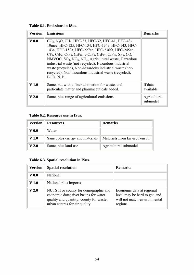
Table 6.1. Emissions in ISus.

Version Emissions Remarks

V 0.0 CO2, N2O, CH4, HFC-23, HFC-32, HFC-41, HFC-43-10mee, HFC-125, HFC-134, HFC-134a, HFC-143, HFC-143a, HFC-152a, HFC-227ea, HFC-236fa, HFC-245ca, CF4, C2F6, C3F8, C4F10, c-C4F8, C5F12, C6F14, SF6, CO, NMVOC, SO2, NOx, NH3, Agricultural waste, Hazardous industrial waste (not-recycled), Hazardous industrial waste (recycled), Non-hazardous industrial waste (not-recycled), Non-hazardous industrial waste (recycled), BOD, N, P.

V 1.0 Same, but with a finer distinction for waste, and particulate matter and pharmaceuticals added.

If data available

V 2.0 Same, plus range of agricultural emissions. Agricultural submodel

Table 6.2. Resource use in ISus.

Version Resources Remarks

V 0.0 Water

V 1.0 Same, plus energy and materials Materials from EnviroConsult.

V 2.0 Same, plus land use Agricultural submodel.

Table 6.3. Spatial resolution in ISus.

Version Spatial resolution Remarks

V 0.0 National

V 1.0 National plus imports

V 2.0 NUTS II or county for demographic and economic data; river basins for water quality and quantity; county for waste; urban centres for air quality

Economic data at regional level may be hard to get, and will not match environmental regions.

54

Table 6.4. Sectoral resolution in ISus.

Version Sectoral resolution Remarks

V 0.0 19 production sectors

V 1.0 57 production sectors, consumption

Some emissions and resource use will have to be interpolated to the sectors.

V 2.0 As above

Table 6.5. Emission and resource use coefficients in ISus.

Version Coefficients Remarks

V 0.0 Constant plus trend extrapolation in selected cases

V 1.0 Income and price elasticities; technological change; price and quantity instruments

V 2.0 Same, plus other instruments

Table 6.6. Scope of ISus.

Version Scope Remarks

V 0.0 Emissions, selected damage costs

V 1.0 Emissions, selected concentrations, selected impacts, selected damage costs

Concentrations and impacts depend on the availability of environmental models.

V 2.0 Emissions, selected concentrations, selected impacts, selected damage costs

Concentrations and impacts depend on the availability of environmental models.

55

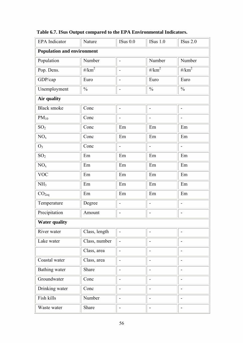
Table 6.7. ISus Output compared to the EPA Environmental Indicators.

EPA Indicator Nature ISus 0.0 ISus 1.0 ISus 2.0

Population and environment

Population Number - Number Number

Pop. Dens. #/km2 - #/km2 #/km2

GDP/cap Euro - Euro Euro

Unemployment % - % %

Air quality

Black smoke Conc - - -

PM10 Conc - - -

SO2 Conc Em Em Em

NOx Conc Em Em Em

O3 Conc - - -

SO2 Em Em Em Em

NOx Em Em Em Em

VOC Em Em Em Em

NH3 Em Em Em Em

CO2eq Em Em Em Em

Temperature Degree - - -

Precipitation Amount - - -

Water quality

River water Class, length - - -

Lake water Class, number - - -

Class, area - - -

Coastal water Class, area - - -

Bathing water Share - - -

Groundwater Conc - - -

Drinking water Conc - - -

Fish kills Number - - -

Waste water Share - - -

56

Surface water Class, share - - -

Waste

Municipal waste Weight - Weight Weight

Share - Share Share

Packaging waste Share Share Share

Bring banks Number - - -

Processing Class, number - - -

Land cover

Land cover Class, area - - Class, area

Urbanisation Class, area - - Class, area

Protected area Share - - Share

Protected species Class, number - - -

Protected birds Class, number - - -

Birds Number - - -

Transport

Vehicles Number - - Number

Size - - Size

Compliance - - -

Age - - Age

Freight Mode, weight - - Mode, weight

CO2 Em Em Em Em

NOx Em Em Em Em

VOC Em Em Em Em

Public transport Number - - Number

Mode, share - - Mode, share

Industry

Production Sector, index Sector, index

Sector, index

Sector, index

Waste Weight Weight Weight Weight

57

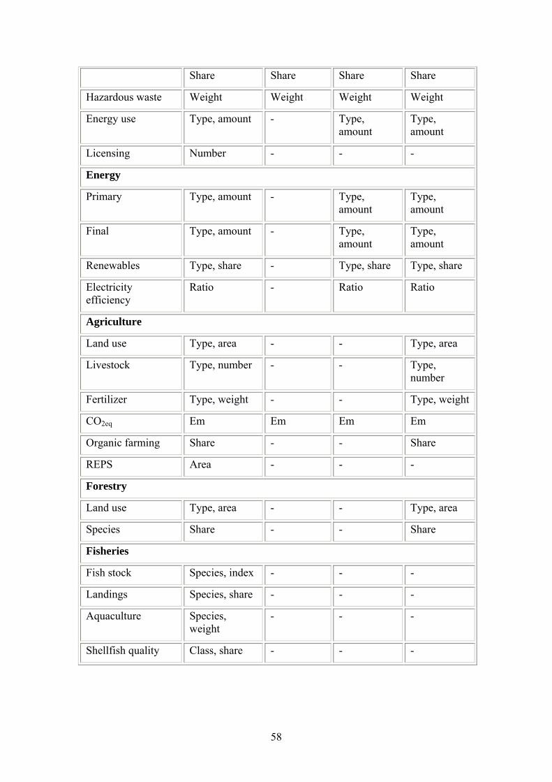
Share Share Share Share

Hazardous waste Weight Weight Weight Weight

Energy use Type, amount - Type, amount

Type, amount

Licensing Number - - -

Energy

Primary Type, amount - Type, amount

Type, amount

Final Type, amount - Type, amount

Type, amount

Renewables Type, share - Type, share Type, share

Electricity efficiency

Ratio - Ratio Ratio

Agriculture

Land use Type, area - - Type, area

Livestock Type, number - - Type, number

Fertilizer Type, weight - - Type, weight

CO2eq Em Em Em Em

Organic farming Share - - Share

REPS Area - - -

Forestry

Land use Type, area - - Type, area

Species Share - - Share

Fisheries

Fish stock Species, index - - -

Landings Species, share - - -

Aquaculture Species, weight

- - -

Shellfish quality Class, share - - -

58

igure 6.1. Structure of ISus0.0.

HERMES

Production

Emissions Emissioncoefficients

Resource use Resource usecoefficients

Damages

Waste Waste generationcoefficients

Recycling

Landfill

F

59


HERMES

Net imports Production Households


Price, quantityinstruments



Concentrations

Impacts

Damages



Recycling

Landfill

Thermal treatment

Net exports

F

60


HERMES

Regional downscaling

Net imports Production Energy Transport Agriculture Households


Price, quantityand otherinstruments



Concentrations

Impacts

Damages



Recycling

Landfill

Thermal treatment

Net exports

F

61

7. Conclusion

This project will develop an Irish Sustainable Development Model (ISus). The model will be capable of linking economic and social developments to their related environmental impacts to provide a tool for policy makers to assess the implications of different growth paths for national objectives on sustainable development. Thus, the eventual purpose of this project is to improve the understanding of economy–environment relationships in Ireland and, in so doing, improve the effectiveness of policy formulation.

As a first step towards the construction of the ISus, this review analysed the state of existing work in this area.

Having introduced the study in Section 1, Section 2 examines the issues surrounding six processes that impact on the environment in Ireland, the effect they can have, how they can be prevented or mitigated, and – perhaps most importantly with a view to constructing the ISus – how each of these is relevant in Ireland.

We establish that these processes have varying impacts on the environment in this country, with waste coming out as a particular concern. Waste is also an area where domestic policy can have significant impact, as opposed to, say, climate change and acidification, where international cooperation is the best solution.

Section 3 presents an overview of existing economic models that have been used in relation to environment-economy interactions, as well as a dedicated discussion of land use modelling. The construction of the ISus will most likely involve many of the methods discussed in this section. For example, the prototype ISus developed by O’Doherty and Tol (2007) took the form of an environmental input-output model, while in its final incarnation the model will link with the ESRI’s HERMES model – an econometric model of the Irish economy. Land use models and scenario analyses are likely to be important also.

All economic models discussed rely to some degree on price information and valuation of the environment. Therefore, Section 4 briefly reviews monetisation methods and their application to environmental resources in Ireland. It was established that valuation studies are few and far between in Ireland. However, a core of literature exists such that validity checks will be available for valuation techniques when they are required in the ISus.

Section 5 presents the data and indicators currently available in Ireland. Ireland could achieve more in terms of its collection of data, but particularly in the organisation and dissemination of data. Although sufficient data existed for O’Doherty and Tol (2007) to construct the prototype ISus for Ireland (ISus0.0), the intention – as outlined in Section 6 - is to expand both the depth and breadth of the model, and thus its data requirements also.

Section 6 examines similar models elsewhere, and also outlines the stages through which the model must progress in order to reach its final specification. An intermediate model (ISus1.0) will provide a finer distinction for waste, add particulate matter and pharmaceuticals emissions, expand the number of resources and sectors analysed by the model, and generally broaden its scope. It is envisaged that the final model (ISus2.0) will be regionalised. It will contain sub-models for agriculture, energy and transport.

62

In conclusion, this review has sought to provide an overview and analysis of existing literature in the area of environmental economics, with a particular focus on those areas that help towards the construction of the ISus, as well as outlining the proposed design for such a model.

It is feasible to construct such a model, and many important insights will be gained from its application. However, the quality of the projections will stand or fall with the quality of the input data.

63

Acknowledgements

The authors would like to acknowledge the contributions of John Curtis, Sue Scott, John Fitz Gerald, Seán Lyons, Edgar Morgenroth, Adele Bergin and Yvonne McCarthy for their input in locating and supplying data, and offering their advice on earlier drafts. Tom Heartel and Steve Rose helped in our understanding of input-output modelling. Finally, we would like to thank Pete Lunn for coming up with the model name.

64

8. Appendix

Index decomposition – mathematical notation

From Ang and Zhang (2000, 1156-59)

Assume that the aggregate energy consumption in industry is the sum of consumption in m different sectors (e.g. food, textiles, metal products, etc.). Define the following variables for time t that are normally measured on an annual basis. Energy consumption is measured in an energy unit and industrial output in a monetary unit.

Et = Total industrial energy consumption

Ei,t = Energy consumption in industrial sector i

Yt = Total industrial production

Yi,t = Production of industrial sector i

Si,t = Production share of sector i (=Yi,t/Yt)

It = Aggregate energy intensity (=Et/Yi,t)

Ii,t = Energy intensity of sector i (=Ei,t/Yi,t)

Express the aggregate energy intensity as a summation of the sectoral data:

(1) ∑=

ititit ISI ,,

where the summation is taken over the m sectors. The aggregate energy intensity is expressed in terms of production structure and sectoral energy intensity.

Suppose the aggregate energy intensity varies from I0 in time 0 to IT in time T. Such a

change may be expressed in two ways: 0I

ID Ttot = and 0III Ttot −=∆ . We refer to the

first as multiplicative decomposition:

int0

DDII

D strt

tot == (2)

where Dstr and Dint respectively give the estimated impacts of structural change and sectoral intensity. The second way is called additive decomposition where the differential change is decomposed into contributions from the same two effects but they appear in the additive form:

65

int0 IIIII strTtot ∆+∆=−=∆ (3)

The above techniques can be applied to decompose changes in total industrial energy consumption. In such a case Eq. (1) is replaced by ∑=

ititiit ISYE ,, , where

multiplicative decomposition takes the form of 0E

ED Ttot = and additive decomposition

the form of 0EEE Ttot −=∆ . The concept is basically the same except that there is an additional term related to the impact of total production Yt, which is known as the production effect in index decomposition terminology.

Laspeyres index method

The Laspeyres index method follows the Laspeyres price and quantity indices in economics by isolating the impact of a variable through letting that specific variable change while holding the other variables at their respective base year values. With reference to Eqs. (1) and (2), the formulae for multiplicative decomposition are:

∑∑

=

iii

iiTi

str IS

ISD

0,0,

0,,

(4)

∑

∑

⎟⎟⎠

⎞⎜⎜⎝

⎛⎟⎟⎠

⎞⎜⎜⎝

⎛

⎟⎟⎠

⎞⎜⎜⎝

⎛⎟⎟⎠

⎞⎜⎜⎝

⎛

=

i

i

ii

ii

year base in the ofintensity Energy

year base in the ofshare Production


T at time ofshare Production

∑∑

=

iii

iTii

IS

ISD

0,0,

,0,

int (5)

∑

∑

⎟⎟⎠

⎞⎜⎜⎝

⎛⎟⎟⎠

⎞⎜⎜⎝

⎛

⎟⎟⎠

⎞⎜⎜⎝

⎛⎟⎟⎠

⎞⎜⎜⎝

⎛

=

i

i

ii

ii



T at time ofintensityEnergy


)( intDDD

Dstr

totrsd = (6)

The residual term Drsd denotes the part of Dtot that is left unexplained. In additive decomposition and with reference to Eqs. (1) and (3), the formulae are:

66

(7) ∑ ∑−=∆i i

iiiTistr ISISI 0,0,0,,

(8) ∑ ∑−=∆i i

iiTi ISISI 0,0,0,int

(9) intIIII strtotrsd ∆−∆−∆=∆

For additive decomposition, some researchers use the concept of percentage change (e.g. Golove and Schipper, 1996; Schipper et al., 1997; and Farla et al., 1998). This is obtained by dividing both sides of Eqs. (7)-(9) by I0:

11)(

0,0,

0,,

0

−=−=∆

∑∑

str

iii

iiTi

str DIS

IS

II

(10)

11)(

0,0,

0,,

0

−=−=∆

∑∑

str

iii

iiTi

str DIS

IS

II

(11)

0

int

000

)()()(II

II

II

II strtotrsd ∆

−∆

−∆

=∆

(12)

Arithmetic mean Divisia index method

The Divisia index is an integral index number introduced by Divisia (1973). More details about this index number can be found in Hulten (1973) and Diewert (1980). Applying the theorem of instantaneous growth rate to Eq. (1) leads to:

∑ ⎥⎦

⎤⎢⎣

⎡+=

i

titii

t

tI

tS

tI

d)ln( d

d)ln( d

d)ln( d ,,ω (13)

where t

tii E

E ,=ω is the sector share of energy consumption and is known as the weight

for sector i in the summation. Integrating over time from 0 to T and rearranging the terms gives:

∫∑∫∑ ⎥⎦

⎤⎢⎣

⎡+⎥

⎦

⎤⎢⎣

⎡=⎟⎟

⎠

⎞⎜⎜⎝

⎛ Tti

i

Tti

it

tI

tII

0

,

0

,

0 d)ln( d

d)ln(S d

ln ωω (14)

67

Exponentiating, Eq. (14) can be expressed in the multiplicative form where:

intDDD strtot =

⎭⎬⎫

⎩⎨⎧

⎥⎦

⎤⎢⎣

⎡= ∫∑

T

i

tiistr t

D0

,

d)ln(S d

exp ω (15)

⎭⎬⎫

⎩⎨⎧

⎥⎦

⎤⎢⎣

⎡= ∫∑

T

i

tii t

D0

,int d

)ln(I dexp ω (16)

Since only discrete data are available in empirical studies, the weight function is often approximated by the arithmetic mean of the weights for year 0 and year T:

⎪⎭

⎪⎬⎫

⎪⎩

⎪⎨⎧

⎟⎟⎠

⎞⎜⎜⎝

⎛+= ∑

0,

,0,, ln2

)(exp

i

Ti

i

iTistr S

SD

ωω (17)

⎪⎭

⎪⎬⎫

⎪⎩

⎪⎨⎧

⎟⎟⎠

⎞⎜⎜⎝

⎛+= ∑

0,

,0,,int ln

2)(

expi

Ti

i

iTi

II

Dωω

(18)

As a result of this approximation (which is also called the Törnqvist formula), the product of Eqs. (17) and (18) is not equal to Dtot and we may write

. The additive Divisia index method can be derived in the same manner. The formulae are:

rsdstrtot DDDD int=

∑ ⎟⎟⎠

⎞⎜⎜⎝

⎛⎟⎟⎠

⎞⎜⎜⎝

⎛+

=∆i i

Ti

i

t

Ti

str SSY

EY

E

I0,

,0

0,,

ln2

(19)

∑ ⎟⎟⎠

⎞⎜⎜⎝

⎛⎟⎟⎠

⎞⎜⎜⎝

⎛+

=∆i i

Ti

i

t

Ti

IIY

EY

E

I0,

,0

0,,

int ln2

(20)

and rsdstrtot IIII ∆+∆+∆=∆ int

68

9. Bibliography

3.9 Section One World Commission on Environment and Development (1987): Our Common Future [Report of the Brundtland Commission]; Oxford; Oxford University Press

3.10 Section Two Adeola, F.O. (2002): Toxic waste in Bisson, K. and J. Proops (eds.): Waste in Ecological Economics; Cheltenham; Elgar

Banister, D. and J. Berechman (2000): Transport investment and economic development; London; UCL Press

Barata, E. (2002): Municipal waste in Bisson, K and J. Proops: Waste in ecological economics; Cheltenham; Edward Elgar

Bascom, R. (1996): Health effects of outdoor air pollution; American Journal of Respiratory and Critical Care Medicine 153(1); pp. 3-50

Baumgärtner, S. (2002): Thermodynamics of waste generation in Bisson, K. and J. Proops (eds.): Waste in Ecological Economics; Cheltenham; Elgar

BBC (2004): Pollution: A Life and death issue [online]; Available from http://news.bbc.co.uk/1/hi/sci/tech/4086809.stm

BBC (2006): Global ecosystems ‘face collapse’ [online]; Available from http://news.bbc.co.uk/1/hi/sci/tech/6077798.stm

Bisson, K. and J. Proops (2002): An Introduction to waste in Bisson, K and J. Proops (eds.): Waste in Ecological Economics; Cheltenham; Elgar

Bowman, J.J. and M. McGettigan (1993): Atmospheric deposition in acid sensitive areas: The Influence of wind direction and a new coal burning electricity generation station on precipitation quality; Water, Air and Soil Pollution 75(1-2); pp. 159-175

Burdett, L., E. Cooksey, I. Christie, W. Wehrmmey, J. Chenoweth and R. Clift (2006): Using science to create a better place: Environment Agency scenarios 2030, Science Report SC050002/SR1, Environment Agency, Bristol.

Carpenter, S.R., N.F. Caraco and V.H. Smith (1998): Nonpoint pollution of surface waters with phosphorus and nitrogen; Ecological Applications 8(3); pp. 559-568

Clancy, L., P. Goodman, H. Sinclair and D.W. Dockery (2002): Effect of air-pollution control on death rates in Dublin, Ireland: An Intervention Study; The Lancet 360(9341); pp. 1210-4

Commission of the European Communities (2005): Thematic strategy on the sustainable use of natural resources [online]; Available from http://ec.europa.eu/environment/natres/pdf/com_natres_en.pdf

DEHLG (2000): National Climate Change Strategy Ireland [online]; Available from http://www.environ.ie/DOEI/DOEIPol.nsf/0/2f96644fae717d7d80256f0f003bc7ec/$FILE/pccexsuminside.pdf

69

DEHLG (2004): Waste management: taking stock and moving forward [online]; Available from http://www.environ.ie/DOEI/doeipub.nsf/0/22eb358f59499ce280256f0f003db978/$FILE/Waste%20Managem.t%20-%20Taking%20St.pdf

EPA (2004): Ireland’s environment 2004 [online]; Available from http://www.epa.ie/NewsCentre/ReportsPublications/IrelandsEnvironment2004/

European Environment Agency (2005): The European environment: State and outlook 2005 [online]; Available from http://reports.eea.europa.eu/state_of_environment_report_2005_1/en/SOER2005_all.pdf

Faber, M., J. Proops and S. Baumgärtner (1998): All production is joint production – a thermodynamic analysis in Faucheux, J, John Gowdy and Isabelle Nicolai: Sustainability and firms: technological change and the changing regulatory environment; Cheltenham; Edward Elgar

HM Treasury (2006): Stern review on the economics of climate change – executive summary [online]; Available from http://www.hm-treasury.gov.uk/media/8AC/F7/Executive_Summary.pdf

Irish Independent (2006): Thirsty capital could soon be drinking from Shannon; 12 October 2006 [online]; Available from http://www.unison.ie/irish_independent/stories.php3?ca=9&si=1703693&issue_id=14749

Künzli, N., R. Kaiser, S. Medina, M. Studnicka, O. Chanel, P. Filliger, M. Herry, F. Horak, Jr, V. Puybonnieux-Texier, P. Quénel: Public-health impact of outdoor and traffic-related air pollution: A European assessment; The Lancet 356(9232); pp. 795-801

Lave L.B. and E.P. Seskin (1970): Air pollution and human health; Science 169(947); pp. 723-33

Mendelsohn, R., W. Morrison, M.E. Schlesinger and N.G. Andronova (2000): Country-specific market impacts of climate change; Climatic Change 45(3-4); pp. 553-569

McCoy, D. (1991): Macroeconomic impact of environmental policy on acid rain in Bradley, J., J. Fitz Gerald and D. McCoy: Medium Term Review; Dublin; ESRI

McGrath, R., E. Nishimura, P. Nolan, T. Semmier, C. Sweeney and S. Wang (2005): Climate change: Regional climate model predictions for Ireland [online]; Available from http://www.c4i.ie/cdi-report-for-web.pdf

Nordhaus, W.D. and J. Boyer (2000): Warming the world: Economic models of global warming; Cambridge; MIT Press

Park, C. (1987): Acid rain: Rhetoric and reality; London; Methuen

Pimm, S.L., G.J. Russell, J.L. Gittleman and T.M. Brooks (1995): The Future of biodiversity; Science 269(5222); pp. 347-350

Simmons, M.R. (2005). Twilight in the desert: The Coming Saudi oil shock and the world economy; New Jersey; Hoboken

Smith, R.A. (1852): On the air and rain of Manchester; Manchester Literary Phil. Soc. Series 2; pp.207–217

70

Tietenberg, T. (1996): Environmental and natural resource economics; New York; Harper Collins

The Economist (2006b): Steady as she goes – Why the world is not about to run out of oil; 20 April 2006 [online]; Available from http://www.economist.com/finance/displaystory.cfm?story_id=E1_GRNPVDG

The Economist (2006a): A Survey of Climate Change; 9 September 2006 [online]; Available from: http://www.economist.com/surveys/displaystory.cfm?story_id=E1_SRVNJNQ

The Irish Times (2003): Downside of one-off rural housing by James Nix, 17 September 2003

The Irish Times (2006): Ireland faces huge Kyoto penalties [online]; Available from http://www.ireland.com/newspaper/ireland/2006/0725/1152913579335.html

Online resources:

Earthtrends: Earthtrends datatables: Energy and resources [online]; Available from http://earthtrends.wri.org/pdf_library/data_tables/ene4_2005.pdf

EEA: Acidification [online]; Available from http://themes.eea.europa.eu/Environmental_issues/acidification

Enfo: Air pollution [online]; Available from http://www.enfo.ie/leaflets/bs13.htm

United Nations Economic Commission for Europe: Convention on Long-range Transboundary Air Pollution [online]; Available from http://www.unece.org/env/lrtap/

UNFCCC: Greenhouse gas inventory data [online]; Available from http://ghg.unfccc.int/index.html

3.11 Section Three

Adams, D., R. Alig, B.A. McCarl, B.C. Murray (2005): FASOMGHG conceptual structure, and specification: Documentation [online]; Available from http://agecon2.tamu.edu/people/faculty/mccarl-bruce/papers/1212FASOMGHG_doc.pdf

Alcamo, J., T. Henrichs and T. Rösch (2000): World water in 2025 – Global modeling scenarios for the World Commission on Water for the 21st century; Report A0002, Centre for Environmental Systems Research, University of Kassel

Ang, B.W. (1994): Decomposition of industrial energy consumption: The Energy intensity approach; Energy Economics 16(3); pp. 163-174

Ang, B.W. (1999): Decomposition methodology in energy demand and environmental analysis in Van den Bergh, J.C.J.M.: Handbook of environmental and resource economics; Cheltenham; Edward Elgar

Ang, B.W. and K.H. Choi (1997): Decomposition of aggregate energy and gas emission intensities for industry: A Refined divisia index method; The Energy Journal 18(3); pp. 59-73

71

Ang, B.W. and F. Zhang (2000): A Survey of index decomposition analysis in energy and environmental studies; Energy 25; pp. 1149-1176

Barker, T. (2000): Ancillary benefits of GHG mitigation in Europe: SO2, NOx and PM10 reductions from policies to meet Kyoto targets using the E3ME model and EXTERNE valuations; Ancillary Benefits and Costs of Greenhouse Gas Mitigation, Proceedings of an IPCC Co-Sponsored Workshop, March, 2000, OECD, Paris

Barrett, A. and J. Lawlor (1995): The Economics of solid waste management in Ireland; Policy Research Series No. 26; Dublin; The Economic and Social Research Institute

Beckerman, W. (1992): Economic growth and the environment: Who’s growth? Who’s environment?; World Development 20(4); pp. 481-496

Behan, J. and K. McQuinn (2002): Projecting net greenhouse gas emissions from Irish agriculture and forestry [online]; Available from http://www.tnet.teagasc.ie/fapri/downloads/esri.pdf

Bergin, A., J. Fitz Gerald and I. Kearney (2002): The Macro-economic effects of using fiscal instruments to reduce Greenhouse Gas Emissions: Final report [online]; Available from http://www.esri.ie/pdf/Sky_JFitz_Paper1.PDF#search=%22%22The%20Macro-economic%20effects%20of%20using%20fiscal%20instruments%20to%20reduce%20Greenhouse%20Gas%20Emissions%22%22

Bergin, A., J. Cullen, D. Duffy, J. Fitz Gerald, I. Kearney and D. McCoy (2003): Medium Term Review: 2003-2010; Dublin; The Economic and Social Research Institute

Böhringer, C. and A. Löschel (2005): Measuring sustainable development: The Use of computable general equilibrium models; ZEW Discussion Paper No. 04-14 [online]; Available from http://ssrn.com/abstract=581381

Boyd, G., J.F. McDonald, M. Ross and D.A. Hanson (1987): Separating the changing composition of U.S. manufacturing production from energy efficiency improvements: A Divisia index approach; Energy Journal 8(2); pp. 77-96

Boyd, G.A., D.A. Hanson and T. Sterner (1988): Decomposition of changes in energy intensity: A comparison of the divisia index and other methods; Energy Economics 10(4); pp. 309-312

Brakman, S., H. Garretsen, and C. van Marrewijk (2001): An Introduction to geographical economics - Trade, location and growth; Cambridge University Press, Cambridge, UK

Brakman, S., H. Garretsen, and M. Schramm (2006): Putting new economic geography to the test: Free-ness of trade and agglomeration in the EU regions; Regional Science and Urban Economics 36; pp. 613-635

Bray, J., S. Hall, A. Kuleshov, J. Nixon and P. Westaway (1995): The Interfaces between policy makers, markets and modellers in the design of economic policy: an intermodel comparison; The Economic Journal 105 (July); pp. 989-1000

Burniaux, J.M., and T.P. Truong (2002): GTAP-E: An Energy-environmental version of the GTAP model; GTAP Technical Paper No. 16, Center for Global Trade Analysis; Purdue University

72

Cambridge Econometrics (2006): E3ME: An Energy-Environment-Economy Model of Europe [online]; Available from http://www.camecon.com/e3me/e3me_model.htm

Charles River Associates International (CRAI): MS-MRT model description [online]; Available from: http://65.198.99.21/documentation/MS-MRT_descr.html

Christaller, W. (1966): Central Places in Southern Germany, Prentice-Hall

Conniffe, D, J. Fitz Gerald, S. Scott, and F. Shortall (1997): The Costs to Ireland of Greenhouse Gas Abatement; Policy Research Series No. 32; Dublin; The Economic and Social Research Institute

Conrad, K. (1999): Computable general equilibrium models for environmental economics and policy analysis in Van den Bergh, J.C.J.M.: Handbook of environmental and resource economics; Cheltenham; Edward Elgar

Cosgrove, W.J. and F. Rijsberman (2000): World water vision: Making water everybody’s interest; London; Earthscan

Darwin, R.F. (1999): A FARMer's view of the Ricardian approach to measuring agricultural effects of climatic change; Climatic Change 41(3-4); pp. 371-411

Darwin, R.F. (2004): Effects of greenhouse gas emissions on world agriculture, food consumption and economic welfare; Climatic Change 66; pp. 191-238

Darwin, R.F. and D. Kennedy (2000): Economic effects of CO2 fertilization of crops: Transforming changes in yield into changes in supply; Environmental Modelling and Assessment 5; pp. 157-168

Darwin, R.F. and R.S.J. Tol (2001): Estimates of the economic effects of sea level rise; Environmental and Resource Economics 19; pp. 113-129

Darwin, R.F., M. Tsigas, J. Lewandrowski and A. Raneses (1995): World agriculture and climate change: Economic adaptations; Agricultural Economic Report 703; US Department of Agriculture Economic Research Service, Washington, D.C.

Dellink, R., M. Bennis and H. Verbruggen (1999): Sustainable economic structures; Ecological Economics 29; pp. 141-154

Department of Public Enterprise (2000): Environmental impacts of Irish transport growth and of related sustainable policies; Report prepared by Oscar Faber Transportation in association with ECOTEC Research & Consulting Ltd., Goodbody Economic Consultants Limited and the Economic and Social Research Institute [online]; Available from: http://www.transport.ie/upload/general/2637.pdf

Dixit, A.K. and J.E. Stiglitz (1977): Monopolistic competition and optimum product diversity; American Economic Review 67(3); pp. 297-308

Don, H. (2004): How econometric models help policy makers: theory and practice; CPB Discussion Paper No 27 [online]; Available from http://www.cpb.nl/eng/pub/cpbreeksen/discussie/27/

Duchin, F. and G.M. Lange (1994): The Future of the environment: ecological economics and technical change; Oxford; Oxford University Press

Duranton, G. (2006): Some foundations for Zipf's Law: Product proliferation and local spillovers; Regional Science and Urban Economics 36; pp. 542-563

73

Edmonds, J., H. Pitcher and R. Sands (2004): Second Generation Model: An Overview [online]; Available from http://www.epa.gov/air/pdfs/SGMoverview.pdf

EEA (2001): Scenarios as tools for international environmental assessments [online]; Available from http://www.usf.uos.de/IA/Scenarios_Report.pdf

Eichammer, W. and W. Mannsbart (1997): Industrial energy efficiency: Indicators for a European cross-country comparison of energy efficiency in the manufacturing industry; Energy Policy 25(7-9); pp. 759-72

Eichner, T. and R. Pethig (2006): Economic land use, ecosystem services, and microfounded species dynamics; Journal of Environmental Economics and Management 52; pp. 707-720

Fankhauser, S. and R.S.J. Tol (2005): On climate change and economic growth; Resource and Energy Economics 27; pp. 1-17

Feenstra, T., H. Cesar and P. Kort (1999): Optimal control theory in environmental economics in Van den Bergh, J.C.J.M.: Handbook of environmental and resource economics; Cheltenham; Edward Elgar

Finnoff, D. and J. Tschirhart (2003): Protecting an endangered species while harvesting its prey in a general equilibrium ecosystem model; Land Economics 79(2); pp. 160-180

Fisher, I. (1972): The Making of index numbers; Boston; Houghton Mifflin

Fitz Gerald, J. (2004): An Expensive way to combat global warming: reform needed in EU emissions trading regime; special article in Quarterly Economic Commentary (The Economic and Social Research Institute), Spring 2004

Fujita, M., P.R. Krugman, and A.J. Venables (1999): The Spatial economy - Cities, regions, and international trade; Cambridge; MIT Press

Gerlagh, R., R. Dellink, M. Hofkes and H. Verbruggen (2002): A Measure of sustainable national income for the Netherlands; Ecological Economics 41.1 (April); pp. 157-174

Greening, L.A. (2004): Effects of human behaviour on aggregate carbon intensity of personal transportation: comparison of 10 OECD countries for the period 1970-1993; Energy Economics 26; pp. 1-30

Greening, L.A., W.B. Davis, L. Schipper and M. Khrushch (1997): Comparison of 6 decomposition methods: application to aggregate energy intensity for manufacturing in 10 OECD countries; Energy Economics 19; pp. 375-390

Gren, I.M., K. Elofsson and P. Jannke (1997), Cost-effective nutrient reductions to the Baltic Sea; Environmental and Resource Economics 10; pp. 341-362.

Harbaugh, W.T., A. Levinson and D. Molloy Wilson (2002): Reexamining the Empirical Evidence for an Environmental Kuznets Curve; Review of Economics and Statistics 84.3 (August); pp. 541-551

Heistermann, M., C. Mueller and K. Ronneberger (2006): Land in sight? Deficits and potentials of continental to global scale land-use modelling; Agriculture, Ecosystems and Environment 114; pp. 141-158

Henderson, J.V. (1974): The Sizes and types of cities; American Economic Review 64(4); pp. 640-656

74

Hertel, T.W., H.L. Lee, S. Rose and B. Sohngen (2006): The Role of global land use in determining greenhouse gas mitigation costs; GTAP Working Paper 36, Global Trade Analysis Project, Purdue University, West Lafayette, IN

HM Treasury (2006): Stern review on the economics of climate change – executive summary [online]; Available from http://www.hm-treasury.gov.uk/media/8AC/F7/Executive_Summary.pdf

Hubacek, K. and J.C.J.M. van der Bergh (2006): Changing concepts of ‘land’ in economic theory: From single to multi-disciplinary approaches; Ecological Economics 56; pp. 5-27

Isard, W. (1956): Location and space-economy; Cambridge; MIT Press

Jansen, H. and G. Klaassen (2000): Economic impacts of the 1997 EU energy tax: simulations with three EU-wide models; Environmental and Resource Economics 15; pp. 179-197

Klaassen M.A.W., D. Vos, A.J. Seebregts, T. Kram, S. Kruitwagen, R.G.J. Huiberts, E.C. van Ierland (1999): Linking an input-output model with MARKAL [online]; Available from http://www.mnp.nl/en/publications/1999/index.html

Krugman, P.R. (1991): Increasing returns and economic geography; Journal of Political Economy 99(3); pp. 483-499

Krugman, P.R. (1998a): What's new about the new economic geography?; Oxford Review of Economic Policy 14(2); pp. 7-17

Krugman, P.R. (1998b): Development, geography, and economic theory; Cambridge; MIT Press

Krzyzanowski, D.A., S. Kypreos, L. Gutzwiller and L. Barreto (2004): Implications of Technology Learning in Energy-Economy Models of the Transport Sector – Report to the Alliance for the Global Sustainability (AGS) [online]; Available from: http://eem.web.psi.ch/Publications/Other_Reports/ReportAGStransport.pdf

Kuhn, A. (2003): From world market to trade flow modelling: The Redesigned WATSIM model; Institute of Agricultural Policy, Market Research, and Economic Sociology, University of Bonn

Leontief, W. (1970): Environmental repercussions and the economic structure: An Input-Output approach; Review of Economics and Statistics 52.3 (August); pp. 262-271

Lewandrowksi, J., R.F. Darwin, M. Tsigas and A. Raneses (1999): Estimating costs of protecting global ecosystem diversity; Ecological Economics 29; pp. 111-125

Loesch, A. (1964): The Economics of Location, New Haven; Yale University Press

Manne, A., Robert Mandelsohn and Richard Richels (1995): A Model for evaluating regional and global effects of GHG reduction policies; Energy Policy 23(1); pp. 17-34

Martin, R. (1999): The New ‘geographical turn’ in economics: Some critical reflections; Cambridge Journal of Economics 23; pp. 65-91

Maskin, E. (1994): The Invisible hand and externalities; The American Economic Review 84(2); pp. 333-337

75

McCarl, B.A. (2004): Forest and agricultural sector optimization model: model description [online]; Available from http://agecon2.tamu.edu/people/faculty/mccarl-bruce/FASOM.html

McQuinn, K., N. O’Donnell and M. Ryan (2005): A Macro-econometric model for Ireland; Research Technical Paper for the Economic Analysis and Research Department, Central Bank and Financial Services Authority of Ireland [online]; Available from http://www.centralbank.ie/data/TechPaperFiles/9RT05.pdf

Meade, J. (1952): External economies and diseconomies in a competitive situation; Economic Journal 62(245); pp. 54-67

Mendelsohn, R.O., W.D. Nordhaus, and D. Shaw (1994): The Impact of climate on agriculture: A Ricardian analysis; American Economic Review 84(4); pp. 753-771

Morovic, T., Gründing, F.J., Jäger, F., Jochem, E., Mannsbart, W., Poppke, H., Schön, M., Tötsch, I.: Energy Conservation Indicators; Berlin; Springer

Morovic, T., G. Gerritse, G. Jaeckel, E. Jochem, W. Mannsbart, H. Poppke, B. Witt: Energy Conservation Indicators II; Berlin; Springer

Nakicenovic, N. and R. Swart [eds] (2000):Intergovernmental Panel on Climate Change special report on emission scenarios [online]; Available from http://www.grida.no/climate/ipcc/emission/

Neary, J.P. (2001): Of hype and hyperbolas: Introducing the new economic geography; Journal of Economic Literature 39(2); pp. 536-561

Nordhaus, W.D. (1992): The “DICE” model: background and structure of a dynamic integrated climate-economy model of the economics of global warming; Cowles Foundation Discussion Paper No 1009 [online]; Available from: http://cowles.econ.yale.edu/P/cd/d10a/d1009.pdf

Nordhaus, W.D. (2006): Geography and macroeconomics: New data and new findings; Proceedings of the National Academy of Science 103(10) [online]; Available from www.pnas.org/cgi/doi/10.1073/pnas.0509842103

Nordhaus, W. and J. Boyer (1999): Warming the World: Economics Models of Global Warming (Internet Edition) [online]; Available from: http://www.econ.yale.edu/%7Enordhaus/homepage/web%20table%20of%20contents%20102599.htm

O’Doherty, J. and R.S.J. Tol (2007): An Environmental input-output model for Ireland; ESRI Working Paper Series 178 [online]; Available from http://www.esri.ie/publications/latest_publications/view/index.xml?id=2152

Pant, H. (2002): Global Trade and Environment Model (GTEM): A computable general equilibrium model of the global economy and environment (a report for the Australian Bureau of Agricultural and Resource Economics, Canberra) [online]; Available from http://www.abareconomics.com/publications_html/models/models/gtem.pdf

Peck, S.C. and T.J. Teisberg (1992): CETA: A Model for carbon emissions trajectory assessment; Energy Journal 13(1); pp. 55-77

Ravetz, J., D. McEvoy, S. Lindley and J. Handley (2003): Linking up: Linking environmental-economic modelling into sustainable planning in Wales and the

76

regions [online]; Available from http://www.sed.manchester.ac.uk/research/cure/downloads/reward_main.pdf

Ricardo, D. (1815): Essay on Profits; Printed for John Murray, Albemarle Street, London

Rosegrant, M.W., S. Meijer and S.A. Cline (2002): International model for policy analysis of agricultural commodities and trade (IMPACT): Model description; International Food Policy Research Institute, Washington, D.C. [online]; Available from http://www.ifpri.org/themes/impact/impactwater.pdf

Rossi-Hansberg, E. (2005): A Spatial theory of trade; American Economic Review 95(5); pp. 1465-1491

Sanchirico, J.N. and J.E. Wilen (1999): Bioeconomics of spatial exploitation in a patchy environment; Journal of Environmental Economics and Management 37; pp. 129-150

Sands, R. and M. Leimbach (2003): Modelling agriculture and land use in an integrated assessment framework; Climatic Change 56; pp. 185-210

Schafer, A. and H. D. Jacoby (2003): Technology detail in a multi-sector CGE model: transport under climate policy; Massachusetts Institute of Technology, Joint Program on the Science and Policy of Global Change: 101; Cambridge (MA)

Schlenker, W., W.M. Hanemann, and A.C. Fisher (2005): Will US agriculture really benefit from global warming? Accounting for irrigation in the hedonic approach; American Economic Review 95(1); pp. 395-406

Scott, S., J. Curtis, J. Eakins, J. Fitz Gerald and J. Hore (2001): Time series and eco-taxes: Energy, Water, Waste; report for EUROSTAT (B1 section. National Accounts methodology, statistics for own resources); Ref KITZ99/274

Scott, S. (2004): Research needs of sustainable development; ESRI Working Paper no. 162

Smith, M.D. and J.E. Wilen (2003): Economic impacts of marine reserves: The Importance of spatial behaviour; Journal of Environmental Economics and Management 46; pp. 183-203

Sohngen, B., R.O. Mendelsohn and R. Sedjo (1999): Forest management, conservation, and global timber markets; American Journal of Agricultural Economics 81; pp. 1-18

Steininger, K.W. (1999): General models of environmental policy and foreign trade in Van den Bergh, J.C.J.M.: Handbook of environmental and resource economics; Cheltenham; Edward Elgar

Stelder, D. (2005): Where do cities form? A Geographical agglomeration model for Europe; Journal of Regional Science 45(4); pp. 657-679

Stern, D.I. (2004): The Rise and fall of the environmental Kuznets curve; World Development 32.8; pp. 1419-1439

Steuart, J. (1767): Inquiry into the principles of political economy; Printed for A. Millar and T. Cadell in the Strand, London

77

Sun, J.W. and P. Malaska (1998): CO2 emission intensity in developed countries 1980-1994; Energy 23(2); pp. 105-112

Timmins, C. (2006): Endogenous land use and the Ricardian valuation of land use; Environmental and Resource Economics 33; pp. 119-142

Tol, R.S.J. (2000): Modelling the costs of emission reduction: different approaches; Pacific-Asian Journal of Energy, 10 (1), 1-7

Torvanger, A. (1991): Manufacturing sector carbon dioxide emissions in nine OECD countries, 1973–87: A Divisia index decomposition to changes in fuel mix, emission coefficients, industry structure, energy intensities and international structure; Energy Economics 13(3); pp. 168-186

Tschirhart, J. (2000): General equilibrium of an ecosystem; Journal of Theoretical Biology 203; pp. 13-32

Turgot, A.R.J. (1793): Reflections on the formation and distribution of wealth; Printed by E. Spragg for J. Good, Bookseller no 159, New Bond Street, John Anderson, no 62, Holborn Hill, and W. Richardson, Royal Exchange, London

van den Bergh, J.C.J.M. and M.W. Hofkes (1999): Economic models of sustainable development in Van den Bergh, J.C.J.M.: Handbook of environmental and resource economics; Cheltenham; Edward Elgar

von Thuenen, J. (1826): The Isolated state; London; Pergamon Press

Verbruggen, H, R.B. Dellink, R. Gerlagh, M.W. Hofkes and H.M.A. Jansen (2001): Alternative calculations of a sustainable national income for the Netherlands according to Hueting in Van Ierland, E.C., J. van der Straaten and H.R.J. Vollebergh: Economic growth and valuation of the environment: a debate; Cheltenham; Edward Elgar

Viguier, L.L., M.H. Babiker and J.M. Reilly: The costs of the Kyoto Protocol in the European Union; Energy Policy 31(5); pp. 459–481

van der Veeren, R.J.H.M. and R.S.J. Tol (2001): Benefits of a reallocation of nitrate emission reductions in the Rhine river basin; Environmental and Resource Economics 18; pp. 19-41.

Warren, R.F. and H.M. ApSimon (2000): Application of limiting marginal abatement costs in optimized strategies to reduce acidification and eutrophication in Europe: Illustrations using the Abatement Strategies Assessment Model (ASAM); Journal of Environmental Assessment Policy and Management 2 (1); pp. 119-166.

Wassenaar, T., P. Gerber, P.H. Verburg, M. Rosales, M. Ibrahim and H. Steinfeld (forthcoming): ‘Projecting land use changes in the neotropics: The Geography of pasture expansion into Forest; Global Environmental Change; Article in press

Weber, A. (1909): Theory of the location of industries; Chicago; University of Chicago Press

Zipf, G.K. (1935): The Psychobiology of language; New York; Houghton-Mifflin

Online Resources:

IEA outline of the MARKAL model available from http://www.etsap.org/markal/main.html

78

OECD glossary of statistical terms [online]; Available from http://stats.oecd.org/glossary/detail.asp?ID=988

Price of a carbon permit from www.pointcarbon.com

3.12 Section Four Campbell, D., G. Hutchinson and R. Scarpa (2006): Using discrete choice experiments to derive individual-specific willingness to pay estimates for landscape improvements under agri-environmental schemes: Evidence from the rural environment protection scheme in Ireland; Nota di Lavoro 26.2006; Fondazione Eni Enrico Mattei, Milan

Campbell, D., G. Hutchinson and R. Scarpa (2006): Lexicographic preferences in discrete choice experiments: Consequences on individual-specific willingness to pay estimates; Nota di Lavoro 128.2006; Fondazione Eni Enrico Mattei; Milan

Campbell, D., G. Hutchinson and R. Scarpa (2006): Integrating landscape improvement indices and discrete choice experiments: Evidence from the Rural Environment Protection Scheme in Ireland; The Rural Economy Research Centre Working Paper Series Working Paper 06-WP-RE-09; University College Galway

Clinch, P. and A. Murphy (2001): Modelling winners and losers in contingent valuation of public goods: appropriate welfare measures and econometric analysis; The Economic Journal 111; pp. 420-443

Curtis, J.A. (2002): Estimating the demand for salmon angling in Ireland; The Economic and Social Review 33(3); pp. 319-332

Fitzpatrick Associates and Coillte (2005): Economic value of trails and forest recreation in the Republic of Ireland: Final report [online]; Available from http://www.coillte.ie/publications/Final%20Economic%20Study%20of%20Trails.pdf

Hynes, S. and N. Hanley (2004): Preservation versus development on Irish rivers: Whitewater kayaking and hydro-power in Ireland; Land Use Policy, 23; pp. 170-180

Hynes, S., C. Buckley and T. van Rensburg (2003): Agricultural versus recreational activity on marginal farmland: A Discrete choice model of recreational activity on Irish farm commonage; The Rural Economy Research Centre Working Paper Series Working Paper 06-WP-RE-03; University College Galway

Hynes, S., N. Hanley and E. Garvey (2004): Up the proverbial creek without a paddle: Accounting for variable participant skill levels in recreational demand modeling; The Rural Economy Research Centre Working Paper Series Working Paper 06-WP-RE-04; University College Galway

Scarpa, R., S. Chilton, G. Hutchinson, and J. Buongiorno (1999): Valuing the recreational benefits from the creation of nature reserves in Irish forests; Ecological Economics 33(2); pp. 237-250

3.13 Section Five Camp Dresser & McKee (2004): Economic analysis of water use in Ireland; Department of the Environment, Heritage and Local Government, Dublin

79

CSO (2006): Environmental accounts for Ireland 1997-2004; Central Statistics Office, Cork

de Haan, M. (1999): On the international harmonisation of environmental accounting: Comparing the national accounting matrix including environmental accounts of Sweden, Germany, the UK, Japan, and the Netherlands; Structural Change and Economic Dynamics 10; pp. 151-160

EPA (no date): Ireland GHG inventory; Environmental Protection Agency, Johnstown Castle [online]; Available from http://coe.epa.ie/ghg/crfdownloads.jsp

EPA (2003): National waste database report 2001; Environmental Protection Agency, Johnstown Castle

EPA (2005): National waste report 2004; Environmental Protection Agency, Johnstown Castle

Hellsten, E., S. Ribacke, and G. Wickbom (1999): SWEEA: Swedish Environmental and Economic Accounts; Structural Change and Economic Dynamics 10; pp. 39-72

Ike, T. (1999): A Japanese NAMEA; Structural Change and Economic Dynamics 10; pp. 123-149

Keuning, S.J., J. van Dalen, and M. de Haan (1999): The Netherlands’ NAMEA: Presentation, usage, and future extensions; Structural Change and Economic Dynamics 10; pp. 15-37

Lenzen, M. and R. Schaeffer (2004): Environmental and social accounting for Brazil; Environmental and Resource Economics 27; pp. 201-226

Nordhaus, W.D. (1999a): The Future of environmental and augmented national accounts: An Overview; Survey of Current Business (November); pp. 45-49

Nordhaus, W.D. and E.C. Kokkelenberg (1999b): Overall appraisal of environmental accounting in the United States; Survey of Current Business (November); pp. 50-65

Nordhaus, W.D. and E.C. Kokkelenberg (eds.) (1999): Nature's numbers: Expanding the national economic accounts to include the environment; Washington, D.C.; National Academy Press


Pedersen, O.G. and M. de Haan (2006): The System of Environmental and Economic Accounts–2003 and the Economic Relevance of Physical Flow Accounting; Journal of Industrial Ecology 10(1-2) [online]; Available from http://www.mitpressjournals.org/doi/pdf/10.1162/108819806775545466

Scott, S. (1999): Pilot environmental accounts, Central Statistics Office, Cork

Stigliani, W.M., F.M. Brouwer, R.E. Munn, R.W. Shaw and M. Antonowsky (1989): Future environments for Europe: some indications of alternative development paths; The Science of Total Environment 80; pp. 1-102

Tjahjadi, B., D. Schaefer, W. Radermacher, and H. Hoeh (1999): Material and energy flow accounting in Germany: Data base for applying the national accounting matrix

80

including environmental accounts concept; Structural Change and Economic Dynamics 10; pp. 73-97

3.14 Section Six Alcamo, J., G.J.J. Kreilman, J.C. Bollen, G.J. van den Born, R. Gerlagh, M.S. Krol, A.M.C. Toet and H.J.M. de Vries (1996a): Baseline scenarios of global environmental change; Global Environmental Change 6(4); pp. 261-304

Alcamo, J. and J.C. Kreileman (1996): Emission scenarios and global climate protection; Global Environmental Change 6(4); pp. 305-334

Bertrand, G., A. Michalski, L. Pench (1999): Scenarios Europe 2010: Five possible futures for Europe; Working Paper of the European Commission Forward Studies Unit [online]; Available from http://ec.europa.eu/comm/cdp/scenario/scenarios_en.pdf

Camp Dresser & McKee (2004): Economic analysis of water use in Ireland; Department of the Environment, Heritage and Local Government, Dublin

CSO (2006): Environmental accounts for Ireland 1997-2004; Central Statistics Office, Cork

EEA (2005a): The European Environment – State and Outlook 2005; European Environment Agency, Copenhagen

EEA (2005b): European Environment Outlook, EEA Report 4/2005, European Environment Agency, Copenhagen

EPA (no date): Ireland GHG inventory; Environmental Protection Agency, Johnstown Castle [online]; Available from http://coe.epa.ie/ghg/crfdownloads.jsp

EPA (2003): National waste database report 2001; Environmental Protection Agency, Johnstown Castle

EPA (2005): National waste report 2004; Environmental Protection Agency, Johnstown Castle

IEA (2006): World Energy Outlook 2006; International Energy Agency, Paris.

IIASA (2006): IIASA-ECS Modeling [online]; Available from http://www.iiasa.ac.at/Research/ECS/docs/models.html

Leemans, R., A. van Amstel, C. Battjes, G.J.J. Kreileman and A.M.C. Toet (1996): The Land cover consequences of large scale utilization of biomass as an energy source; Global Environmental Change 6(4); pp. 335-358


Nakicenovic, N. (ed.) (2000): Global greenhouse gas emissions scenarios: Integrated modeling approaches; Technological Forecasting and Social Change 63(2-3)

Nakicenovic, N. and R.J. Swart (eds.) (2001): Emission Scenarios 2000 – Special Report of the Intergovernmental Panel on Climate Change; Cambridge; Cambridge University Press

81

Scott, S. (1999): Pilot environmental accounts, Central Statistics Office, Cork

3.15 Appendix Ang, B.W. and F. Zhang (2000): A Survey of index decomposition analysis in energy and environmental studies; Energy 25; pp. 1149-1176.

82

Year Number Title/Author(s) ESRI Authors/Co-authors Italicised

2007

185

Managing Term-Time Employment and Study in Ireland Merike Darmody and Eme Smyth r

184

The Effects of Human Capital on Output Growth in ICT Industries: Evidence from OECD Countries Gavin Murphy and Iulia Traistaru Siedschlag -

.

r .

.

.J

183

Real Interest Parity in the EU and the Consequences for Euro Area Membership: Panel Data Evidence, 1979-2005 Martin O’Brien

182

Can Small Firms’ Perceived Constraints Help Explain Survival Rates? Seán Lyons

181

Understanding the Implications of Choice of Deprivation Index for Measuring Consistent Poverty in Ireland Christopher T. Whelan

180

Economics in Ireland Frances Ruane and Richard S.J Tol

179

Airline Emissions of Carbon Dioxide in the European Trading System John Fitz Gerald and Richa d S.J Tol

178 An Environmental Input-Output Model for Ireland Joe O’Doherty and Richard S.J Tol

2006 177 The Impact of a Carbon Tax on International Tourism Richard S . Tol

176 Economic Integration and Structural Change: The Case of Irish Regions Edgar Morgenroth

175 Macroeconomic Differentials and Adjustment in the Euro Area Iulia Traistaru-Siedschlag

174 The Impact of Climate Change on Tourism in Germany, The UK and Ireland: A Simulation Study Jacqueline M. Hamilton and Richard S.J. Tol

83

173 Regional Growth Cycle Synchronisation with the Euro Area Gabriele Tondl and Iulia Traistaru-Siedschlag

172 Measuring Material Deprivation with EU-SILC: Lessons from the Irish Survey Christopher T. Whelan and Bertrand Maî re t

t

r

t

171 Levels and Patterns of Material Deprivation in Ireland:

After the 'Celtic Tiger' Christopher T. Whelan and Bertrand Maî re

2005 169 The Case for an EU-wide Measure of Poverty Tony Fahey

168 Market Size, Market Structure & Market Power in the Irish Electricity Industry N. McCarthy

167 An Integrated Micro-Macro (IMM) Approach to the Evaluation of Large-scale Public Investment Programmes: The Case of EU Structural Funds John Bradley and T. Mitze, Edgar Morgenroth, G. Untiedt

166 Rising House Prices in an Open Labour Market David Duffy and J. Fitz Ge ald, I. Kearney

165 Measuring Consistent Poverty in Ireland with EU SILC Data Christopher T. Whelan and Brian Nolan, Bertrand Maître

164 Income, Deprivation and Economic Strain in the Enlarged European Union Christopher T. Whelan and Bertrand Maî re

2004 163 Living in Ireland Survey – Technical Report and Codebook for Data Users Dorothy Watson

162 Research Needs of Sustainable Development Sue Scott

161 Generation Adequacy in an Island Electricity System John Fitz Gerald

160 Energy Policy in Ireland John Fitz Gerald

84

Irish Sustainable Development Model (ISus) Literature ...

Documents

Transcript of Irish Sustainable Development Model (ISus) Literature ...