IPTS CAPRI Documentation - uni-bonn.de · PDF fileCAPRI Documentation Page 3 of 133...

CAPRI Modelling System Documentation COMMON AGRICULTURAL POLICY REGIONAL IMPACT ANALYSIS Editor: Wolfgang Britz “Development of a regionalised EU-wide operational model to assess the impact of current Common Agricultural Policy on farming sustainability”, J05/30/2004 – Deliverable 1 Bonn, August 2005

CAPRI Documentation

of 133

CAPRI Modelling System Documentation COMMON AGRICULTURAL POLICY REGIONAL IMPACT ANALYSIS Editor: Wolfgang Britz With contributions of: Marcel Adenäuer, Bonn Jose-Maria Alvarez-Coque, Valencia Wolfgang Britz, Bonn Kamel Elouhichi Guillermo Flichman Eoghan Garvey, Galway Thomas Heckelei, Bonn Bruno Henry de Frahan Torbjörn Jansson, Lund & Bonn Guiseppe Palladino, Reggio Emilia Ignacio Perez, Bonn Marco Setti, Reggio Emilia Christine Wieck, Bonn

CAPRI Documentation

of 133

Acknowledgements Many people and institutions contributed in many different ways over the years to the development of the CAPRI modelling system. Prof. Henrichsmeyer should be named first, as he pushed the team in Bonn to look for suitable partners, start pre-tests and wrote a proposal using the idea of a combination of a EU market model for agricultural products with regional aggregate programming models, which led to the first CAPRI project 1996-1999. The work would have not been possible without the experience and tools developed in the context of earlier projects by team members in Bonn such as Hans-Josef Greuel and Andrea Zintl. Equally important were elements of the SPEL/MFSS and RAUMIS projects. In the latter case, some of the RAUMIS team members contributed directly to the first CAPRI project.

Next comes the team in Reggio Emilia who invented the acronym CAPRI – a good trademark is almost as important as the product itself. It is certainly fair to mention the European Commission next, which provided the necessary additional funds beyond the ones invested by the network itself. But the role of the European Commission went beyond that in many respects. The success of CAPRI would have been impossible without the interest and critical feedback of our partners at DG-AGRI in G1 and G2. Additionally, bigger parts of the data part were provided by EUROSTAT and contacts at EUROSTAT brought critical and helpful comments to the development of the new methodology and algorithm to build up a consistent and complete data base. DG-ENV financed another project around CAPRI and the European Environmental Agency opted for CAPRI as the source for the herd size projection in the context of the Clean Air for Europe program.

Remain the many people who contributed with bits and pieces over the years. It is not necessary here to mention them individually, many can be found as authors of parts of this documentation anywhere. But it seems important to stress the fact that their ability to look at the bright side of life, to see the potential of ideas more than the hard work required to get them working, and to remain friendly and helpful even under stress made the CAPRI network a unique experience for all involved.

The next round of CAPRI projects – again funded by DG-RSRCH – has already started. The editor hopes that the success of the project will continue as the fun to work together with a devoted network of researchers, in many cases, now friends.

CAPRI Documentation

of 133

Table of Contents Table of Contents 4

1 Introduction 7 1.1 Structure of the documentation 7 1.2 History of CAPRI 7 1.3 Overview on CAPRI 8

2 The CAPRI Data Base 11 2.1 Production Activities as the core 12 2.2 Linking production activities and the market 13 2.3 The Complete and Consistent Data Base (COCO) for the national scale 15

2.3.1 Overview and data requirements for the national scale 15 2.3.2 Estimation procedure 15 2.3.3 Defining upper and lower bounds for the estimated value 18 2.3.4 Concluding remark on the estimation process 22 2.3.5 Data and estimation groups 22 2.3.6 Consistent estimation of hectares, yields and gross production 23 2.3.7 Consistency of the farm and market balances for crop products 24 2.3.8 Consistency of herd sizes, animal production and balance sheets 28

2.4 The Regionalised Data Base (CAPREG) 31 2.4.1 Data requirements at regional level 31 2.4.2 Data sources at regional level 31 2.4.3 Data availability at regional level 31 2.4.4 Reading and storing the original REGIO data 32 2.4.5 Methodological proceeding 32 2.4.6 Prices for outputs and inputs 33 2.4.7 Filling gaps in REGIO 33 2.4.8 Mapping crop areas and herd sizes from REGIO to COCO definitions 34 2.4.9 Perfect aggregation between regional and national data for activity levels 34 2.4.10 Estimating expected yields with a Hodrick-Prescott filter 36

2.5 The world Data Base 36

3 Input Allocation 37 3.1 Input allocation excluding young animals, fertiliser and feed 37

3.1.1 Background 37 3.1.2 Econometric Estimation 38 3.1.3 Reconciliation of Inputs, using Highest Posterior Density Estimators 40 3.1.4 Highest Posterior Density estimation framework 42 3.1.5 How are the results used in CAPRI? 43

3.2 Input allocation for young animals and the herd flow model 44 3.3 Input allocation for feed 46

3.3.1 Estimation of fodder prices 46 3.3.2 Feed input coefficients 48

3.4 Input allocation for fertilisers and nutrient balances 58 3.4.1 Nutrient balances for NPK 59 3.4.2 NPK output at tail 59

CAPRI Documentation

of 133

3.4.3 The ammonia module 62 3.4.4 Input allocation of organic and inorganic NPK and the nutrient balance 63 3.4.5 Greenhouse Gases 68

4 Baseline Generation Model (CAPTRD) 71 4.1 Trend curve 72 4.2 Consistency constraints in the trend projection tool 73

4.2.1 Constraints relating to market balances and yields 73 4.2.2 Constraints relating to agricultural production 74 4.2.3 Constraints relating to prices, production values and revenues 74 4.2.4 Constraints relating to consumer behaviour 75 4.2.5 Constraints relating to processed products 75 4.2.6 Constraints relating to policy 76 4.2.7 Constraints relating to growth rates 76

4.3 Three-stage procedure for trends 77 4.3.1 Step 1: Unrestricted trends 77 4.3.2 Step 2: Constrained trends at Member State level 77 4.3.3 Step 3: Adding supports based on external results and breaking down to regional level 79 4.3.4 Breaking down results from Member State to regional level 80

4.4 Calibrating the model to the projection 80 4.4.1 Calibrating the regional supply models 80 4.4.2 Calibrating the global trade model 81

5 Simulation Scenario Model (CAPMOD) 83 5.1 Overview of the system 83 5.2 Module for agricultural supply at regional level 85

5.2.1 Basic interactions between activities in the supply model 85 5.2.2 Detailed discussion of the equations in the supply model 87 5.2.3 Calibration of the regional programming models 91 5.2.4 Estimating the supply response of the regional programming models 91

5.3 Market module for young animals 92 5.4 Market module for agricultural outputs 92

5.4.1 Overview on the market model 92 5.4.2 The approach of the CAPRI market module 95 5.4.3 Behavioural equations for supply and feed demand 96 5.4.4 Behavioural equations for final demand 96 5.4.5 Behavioural equations for the processing industry 98 5.4.6 Trade flows and the Armington assumption 99 5.4.7 Market clearing conditions 101 5.4.8 Price linkages 101 5.4.9 Endogenous policy instruments in the market model 102 5.4.10 Endogenous tariffs under Tariff Rate Quotas 104 5.4.11 Overview on a regional module inside the market model 104 5.4.12 Basic interaction inside the market module during simulations 105

5.5 Parameter calibration and sources for the behavioural equations 106 5.5.1 Calibration of the system of supply functions 106 5.5.2 Calibration of the final demand systems 106

5.6 Linking the different modules – the price mechanism 107 5.7 Sensitivity of the CAPRI model to the Armington substitution elasticities 108

6 Farm Type Programming Model: a FADN-based approach 113

CAPRI Documentation

of 133

6.1 The CAPRI farm type approach 113

7 CAPRI Exploitation tools 120

References 123

Annex: Code lists 124

CAPRI Documentation

of 133

1 Introduction

1.1 Structure of the documentation

The documentation is structured as follows. The short introduction in chapter 1 first gives an overview of the CAPRI activities followed by a short description of the system. The rest of the document follows the project workflow: the different steps of building up the national and regional data base (chapter 2), the allocation of different inputs (chapter 3) and the projection tools needed to establish a baseline (chapter 4) are discussed. Chapter5 deals with the scenario impact analysis: description of the different modules of the economic model and their relationships. In the last two chapters (chapters 6 and 7) the farm type approach and the exploitation tools used in CAPRI are briefly presented.

1.2 History of CAPRI

CAPRI stands for ‘Common Agricultural Policy Regionalised Impact analysis’ and is both the acronym for an EU-wide quantitative agricultural sector modelling system and of the first project centred around it1. The name hints at the main objective of the system: assessing the effect of CAP policy instruments not only at the EU or Member State level but at sub-national level as well.

The scope of the project has widened over time: the first phase (FAIR3-CT96-1849: CAPRI 1997-1999) provided the concept of the data base and the regional supply models, but linked these to a simple market model distinguishing the EU and rest-of-the-world. In parallel, a team at the FAL in Braunschweig applied CAPRI to asses the consequences of an increased share of biological farming system (FAIR3-CT96-1794: Effects of the CAP-reform and possible further developments on organic farming in the EU). A further, relatively small project (ENV.B.2/ETU/2000/073: Development of models and tools for assessing the environmental impact of agricultural policies, 2001-2002) added a dis-aggregation below administrative regions in form of farm type models, refined the existing environmental indicators and added new ones. A new project with the original network (QLTR-2000-00394: CAP-STRAT 2001-2004) refined many of the approaches of the first phase, and linked a complex spatial global multi-commodity model into the system. The application of CAPRI for sugar market reform options in the context of another project improved the way the complex ABC sugar quota system is handled in the model.

In 2004, again a larger project (FP VI, Nr. 501981: CAPRI-Dynaspat) started under the co-ordination of the team in Bonn to render the system recursive-dynamic, dis-aggregate results in space, include the new Member States and add a labour module and an indicator for energy use. At the same time, a project began to apply CAPRI to analyse the effects of bi-lateral trade liberalisation with Mediterranean countries (FP VI, Nr. 502457: EU-MedAgPol). In 2005, a project for IPTS/JRC started to update and improve the farm type model layer and to include Bulgaria and Romania. At the same time, the SEAMLESS project (FP VI: 2005-2009) started, with CAPRI used to link results with a complex layer of farm type models and from there to national, EU and global markets. In SEAMLESS the farm type layer of CAPRI will be refined and updated, and a module for endogenous structural change

1 Web Site: http://www.agp.uni-bonn.de/agpo/rsrch/capri/capri_e.htm.

CAPRI Documentation

of 133

is foreseen. In parallel, the team in LEI, The Hague, The Netherlands, will apply CAPRI in the integrated project SENSOR (2005-2008).

During the years, the system was applied to a wide range of different scenarios. The very first application in 1999 analysed the so-called ‘Agenda 2000’ reform package of the CAP. Shortly afterwards, a team at SLI, Lund, Sweden applied CAPRI to analyse CAP reform option for milk and dairy. FAL, Braunschweig looked into the effects of an increase of biological production systems. WTO scenarios were run by the team in Bonn in 2002 and 2005. Moreover, CAPRI was applied to analyse sugar market reform options at regional level, linked to results of the WATSIM and CAPSIM models. In 2003, scenarios dealing with the CAP reform package titled ‘Mid Term Review’ were performed by the team in Bonn (Britz et al. 2003) and tradable permits for greenhouse gas emission from agriculture analysed (Pérez 2005). The team in Louvain-La-Neuve, together with the group in Bonn, analysed sugar market reform options, applying the market module linked to the regional supply models (Adenaeuer et al. 2004). In 2004 followed an analysis of a compulsory insurance paid by farm against Food and Mouth disease by SLI and runs dealing with methane emission by the team in Galway, Ireland. In the same year, CAPRI was installed by DG-AGRI in Brussels and a baseline generated in order to match DG-AGRI’s outlook projections.

Three teams should be mentioned, as they provided their own funds to share the network and contribute to the system: the teams at FAT, Tänikon in Switzerland, the team at NILF, Oslo in Norway, and the team at SLI, Lund in Sweden. If not explicitly mentioned in the following, the documented features had been co-financed by DG-RSRCH. The documentation as it stands now captures the state of the system in spring 2004 at the end of the CAP-STRAT project. It is planned to update the documentation on a regular basis if the need arises.

1.3 Overview on CAPRI

The CAPRI modelling system itself consists of specific data bases, a methodology, its software implementation and the researchers involved in their development, maintenance and applications.

The data bases exploit wherever possible well-documented, official and harmonised data sources, especially data from EUROSTAT, FAOSTAT, OECD and extractions from the Farm Accounting Data Network (FADN)2. Specific modules ensure that the data used in CAPRI are mutually compatible and complete in time and space. They cover about 50 agricultural primary and processed products for the EU (see table 26 in the Annex), from farm type to global scale including input and output coefficients.

The economic model builds on a philosophy of model templates which are structurally identical so that instances for products and regions are generated by populating the template with specific parameter sets. This approach ensures comparability of results across products, activities and regions, allows for low cost system maintenance and enables its integration within a large modelling network such as SEAMLESS. At the same time, the approach opens up the chance for complementary approaches at different levels, which may shed light on different aspects not covered by CAPRI or help to learn about possibility aggregation errors in CAPRI.

2 FADN data are used in the context of so-called study contracts with DG-AGRI, which define explicitly the scope for which the data can be used, who has access to the data and ensure the data are destroyed after the lifetime of the contract.

CAPRI Documentation

of 133

The economic model is split into two major modules. The supply module consists of independent aggregate non-linear programming models representing activities of all farmers at regional or farm type level captured by the Economic Accounts for Agriculture (EAA). The programming models are a kind of hybrid approach, as they combine a Leontief-technology for variable costs covering a low and high yield variant for the different production activities with a non-linear cost function which captures the effects of labour and capital on farmers’ decisions. The non-linear cost function allows for perfect calibration of the models and a smooth simulation response rooted in observed behaviour. The models capture in high detail the premiums paid under CAP, include NPK balances and a module with feeding activities covering nutrient requirements of animals. Main constraints outside the feed block are arable and grassland, set-aside obligations and milk quotas. The complex sugar quota regime is captured by a component maximising expected utility from stochastic revenues. Prices are exogenous in the supply module and provided by the market module. Grass, silage and manure are assumed to be non-tradable and receive internal prices based on their substitution value and opportunity costs.

The market module consists of two sub-modules. The sub-module for marketable agricultural outputs is a spatial, non-stochastic global multi-commodity model for about 40 primary and processed agricultural products, covering about 40 countries or country blocks in 18 trading blocks (table 19 on page 94). Bi-lateral trade flows and attached prices are modelled based on the Armington assumptions (Armington 1969). The behavioural functions for supply, feed, processing and human consumption apply flexible functional forms where calibration algorithms ensure full compliance with micro-economic theory including curvature. The parameters are synthetic, i.e. to a large extent taken from the literature and other modelling systems. Policy instruments cover Product Support Equivalents and Consumer Support Equivalents (PSE/CSE) from the OECD, (bi-lateral) tariffs, the Tariff Rate Quota (TRQ) mechanism and, for the EU, intervention stocks and subsidized exports. This sub-module delivers prices used in the supply module and allows for market analysis at global, EU and national scale, including a welfare analysis. A second sub-module deals with prices for young animals.

As the supply models are solved independently at fixed prices, the link between the supply and market modules is based on an iterative procedure. After each iteration, during which the supply module works with fixed prices, the constant terms of the behavioural functions for supply and feed demand are calibrated to the results of the regional aggregate programming models aggregated to Member State level. Solving the market modules then delivers new prices. A weighted average of the prices from past iterations then defines the prices used in the next iteration of the supply module. Equally, in between iterations, CAP premiums are re-calculated to ensure compliance with national ceilings.

CAPRI allows for modular applications as e.g. regional supply models for a specific Member State may be run at fixed exogenous prices without any market module. The farm type model layer may be switched ON or OFF. Equally, the model may be used in a comparative-static or recursive-dynamic fashion.

Post-model analysis includes the calculation of different income indicators as variable costs, revenues, gross margins, etc., both for individual production activities as for regions, according to the methodology of the EAA. A welfare analysis at Member State level, or globally, at country or country block level, covers agricultural profits, tariff revenues, outlays for domestic supports and the money metric measure to capture welfare effects on consumers. Outlays under the first pillar of the CAP are modelled in very high detail. Environmental indicators cover NPK balances and output of climate relevant gases according the guidelines of the Intergovernmental Panel on Climate Change (IPCC). Model results are presented as

CAPRI Documentation

of 133

interactive maps and as thematic interactive drill-down tables. These exploitation tools are further explained in the last chapter.

The technical solution of CAPRI is centred on the modelling language GAMS which is applied for most of the data base work and CONOPT applied as solver for the different constrained (optimisation) problems. The different modules are steered by a Graphical User Interface currently realised in C, which interacts with FORTRAN code and libraries which are inter-alias dealing with data base management. Typically, these applications generate run-specific parts of the GAMS code. Exploitation tools apply additionally Java applets for interactive maps and XLM/XSLT to generate interactive HTML tables.

Methodological development, updating, maintenance and application of CAPRI are based on a network approach with is currently centred in Bonn. The team in Bonn acts as a ‘clearing house’: any changes introduced in CAPRI are reviewed by it and, when accepted, become part of the master version. The master version, covering data bases, software and documentation is distributed to all participants of the network usually in the context of training sessions which bring the network together at least once per year. The CAPRI modelling system may be defined as a ‘club good’: there are no fees attached to its use but the entry in the network is controlled by the current club members. The members contribute by acquiring new projects, by quality control of data, new methodological approaches, model results and technical solutions, and by organising events such as project meetings or training sessions. So far, the network approach worked quite successfully but it might need revision if the club exceeds a certain size.

CAPRI Documentation

of 133

2 The CAPRI Data Base

Models and data are almost not separable. Methodological concepts can only be put to work if the necessary data are available. Equally, results obtained with a model mirror the quality of the underlying data. The CAPRI modelling team consequently invested considerable resources to build up a data base suitable for the purposes of the project. From the beginning, the idea was to create wherever possible sustainable links to well-established statistical data and to develop algorithms which can be applied across regions and time, so that an automated update of the different pieces of the CAPRI data base could be performed as far as possible.

The main guidelines for the different pieces of the data base are:

• Wherever possible link to harmonised, well documented, official and generally available data sources to ensure wide-spread acceptance of the data and their sustainability.

• Completeness over time and space. As far as official data sources comprise gaps, suitable algorithm were developed and applied to fill these.

• Consistency between the different data (closed market balances, perfect aggregation from lower to higher regional level etc.)

• Consistent link between ‘economic’ data as prices and revenues and ‘physical data’ as farm and market balances, crop rotations, herd sizes, yields and input demand.

According to the different regional layers interlinked in the modelling system, data at Member State level -currently EU27 plus Norway- need to fit to data at regional level -administrative units at the so-called NUTS 2 level, about 300 regions for EU25- and data at global level, currently 16 non-EU regions broken down to 27 countries or country blocks. As it would be impossible to ensure consistency across all regional layers simultaneously, the process of building up the data base is split in three main parts:

• Building up the data base at national or Member State level. It integrates the EAA (valued output and input use) with market and farm data, with crop rotations and herd sizes and a herd flow model for young animals (section 0).

• Building up the data base at regional or NUTS 2 level, which takes the national data as given (for purposes of data consistency), and includes the allocation of inputs across activities and regions as well as consistent acreages, herd sizes and yields at regional level. The input allocation step allows the calculation of regional and activity specific economic indicators such as revenues, costs and gross margins per hectare or head. The regionalisation step introduces supply oriented CAP instruments like premiums and quotas (section 2.4).

• Building up the global data base, which includes supply utilisation accounts for the other regions in the market model, bilateral trade flows, as well as data on trade policies (Most Favourite Nation Tariffs, Preferential Agreements, Tariff Rate quotas, export subsidies) plus data domestic market support instruments (market interventions, subsidies to consumption) (section 2.5).

The basic principle of the CAPRI data base is that of the ‘Activity Based Table of Accounts’ which roots in the combination of a physical and valued input/output table including market balances, activity levels (acreages and herd sizes) and the EAA. The concept was developed

CAPRI Documentation

of 133

end of seventies building on similar approaches at the farm level at the Institute for Agricultural Policy in Bonn and first applied in the so-called SPEL/EU data base.

2.1 Production Activities as the core

The economic activities in the agricultural sector are broken down conceptually into ‘production activities’ (e.g. cropping a hectare of wheat or fattening a pig). These activities are characterised by physical output and input coefficients. For most activities, total production quantities can be found in statistics and output coefficients derived by division of activity levels (e.g. ‘soft wheat’ would produce ‘soft wheat’ and ‘straw’, whereas ‘pigs for fattening’ would produce ‘pig meat’ and NPK comprised in manure). However, for some activities other sources of information are necessary (e.g. carcass weights of sows is necessary to derive the output coefficient for the pig fattening process). For manure output engineering functions are used to define the output coefficients. The way the different output coefficients are calculated is described in more detail below.

The second part characterising the production activities are the input coefficients. Soft wheat, to pick up our example again, would be linked to a certain use of NPK fertiliser, to the use of plant protection inputs, repair and energy costs. All these inputs are used by many activities, and official data regarding the distribution of inputs to activities are not available. The process of attributing total input in a region to individual activities is called input allocation. It is methodologically more demanding than constructing output coefficients. Specific estimators are developed for young animals, fertilisers, feed and the remaining inputs, which are discussed below.

Multiplied with average farm gate prices for outputs and inputs respectively, output coefficients define farm gate revenues, and input coefficients variable production costs. The average farm prices used in the CAPRI data base are derived from the EEA and hence link physical and valued statistics. However, in some cases as young animals and manure which are not valued in the EEA, own estimates are introduced.

In order to finalise the characterisation of the income situation in the different production activities, subsidies paid to production must be taken into account. The CAPRI data base features a rather complex description of the different CAP premiums allocated to the individual activities. However, the problem of subsidies outside of CAP for the EU Member States remains so far unsolved, but is on the agenda for future ameliorations.

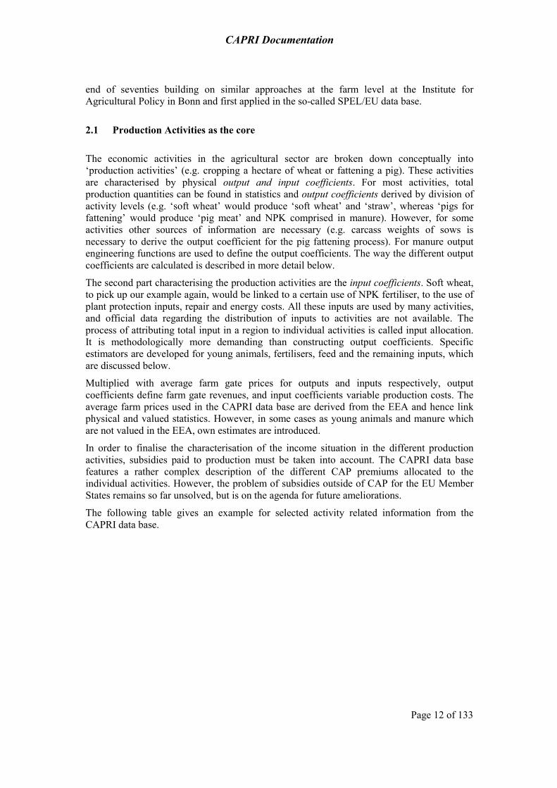
The following table gives an example for selected activity related information from the CAPRI data base.

CAPRI Documentation

of 133

Table 1 Example of selected data base elements for a production activity

SW HE [Soft w heat production activity]

Description Unit

OutputsSWHE 7853.84 Soft wheat yield kg/haSTRA 9817.30 Straw yield kg/haInputsNITF 175.52 Organic and anorganic N applied kg/haPHOF 49.57 Organic and anorganic P applied kg/haPOTF 62.51 Organic and anorganic K applied kg/haSEED 70.91 Seed input const Euro 1995/haPLAP 59.85 Plant protection products const Euro 1995/haREPA 53.27 Repair costs const Euro 1995/haENER 25.15 Energy costs const Euro 1995/haINPO 79.25 Other inputs const Euro 1995/haIncome indicatorsTOOU 825.26 Value of total outputs Euro/haTOIN 522.13 Value of total inputs Euro/haGVAP 303.13 Gross value added at producer prices Euro/haPRME 328.86 CAP premiums Euro/haMGVA 631.99 Gross value added at producer prices plus

premiumsEuro/ha

Activity level and data re lating to CAPLEVL 609.91 Hectares cropped 1000 haHSTY 5.22 Historic yield used to define CAP premiums t/haSETR 8.63 Set aside rate %Source: CAPRI data base, Denmark, three year average 2000-2002

2.2 Linking production activities and the market

The connection between the individual activities and the markets are the activity levels. Total soft wheat produced is the sum of cropped soft wheat hectares multiplied with the average soft wheat output coefficient. In cases like pig meat, as mentioned before, several activities are involved to derive production.

The produced quantities enter the farm and market balances. Production plus imports as the resources are equal to the different use positions as exports, stock changes, feed use, human consumption and processing. These balances are only available at Member State, not at regional level. Production establishes the link to the EAA as well, as average farm gate prices are unit values derived by dividing the values from the EAA by production quantities.

The three basic identities linking the different elements of the data base are expressed in mathematical terms as following. The first equation implies that total production or total input use (code in the data base: GROF or gross production/gross input use at farm level) can be derived from the input and output coefficients and the activity levels (LEVL):

Equation 1 ∑=j

jjio IOLEVLGROF

The second type of identities refers to the farm and market balances:

CAPRI Documentation

of 133

Equation 2 io io io io io

io io io io io io

io io io io

GROF SEDF LOSF INTF NETFNETF IMPT EXPT STCM FEDM LOSM

SEDM HCOM INDM PRCM

− − − =+ = + + +

+ + + +

The farm balance positions are seed use (SEDF) and losses (LOSF) on farm (only reported for cereals) and internal use on farm (INTF, only reported for manure and young animals). NETF or net trade on farm is hence equal to valued production/input use and establishes the link between the market and the agricultural production activity. Adding imports (IMPT) to NETF defines total resources, which must be equal to exports (EXPT), stock changes (STCM), feed use on market (FEDM), losses on market (LOSM), seed use on market (SEDM), human consumption (HCOM), industrial use (INDM) and processing (PRCM).

The third identity defines the value of the EAA in producer prices (EAAP) as sold production or purchased input use (NETF) in physical terms multiplied with the unit valued price (UVAP):

Equation 3 ioioio NETFUVAPEAAP =

The following table shows the elements of the CAPRI data base as they have been arranged in the tables of the data base.

Table 2 Main elements of the CAPRI data base

Activities Farm- and market balances

Prices Positions from the EAA

Outputs Output coefficients Production, seed and feed use, other internal use, losses, stock changes, exports and imports, human consumption, processing

Unit value prices from the EAA with and without subsidies and taxes

Value of outputs with or without subsidies and taxes linked to production

Inputs Input coefficients Purchases, internal deliveries

Unit value prices from the EAA with and without subsidies and taxes

Value of inputs with or without subsidies and taxes link to input use

Income indicators

Revenues, costs, Gross Value Added, premiums

Total revenues, costs, gross value added, subsidies, taxes

Activity levels Hectares, slaughtered heads or herd sizes

Secondary products

Marketable production, losses, stock changes, exports and imports, human consumption, processing

Consumer prices

CAPRI Documentation

of 133

2.3 The Complete and Consistent Data Base (COCO) for the national scale

2.3.1 Overview and data requirements for the national scale

The CAPRI modelling system is, as far as possible, fed by statistical sources available at European level which are mostly centralised and regularly updated. Farm and market balances, economic indicators, acreages, herd sizes and national input output coefficients are almost entirely taken from EUROSTAT. In order to use this information directly in the model, the CAPRI and CAPSIM3 teams developed out of EUROSTAT data a complete and consistent data base (COCO) at Member State level (Britz et al. 2002).

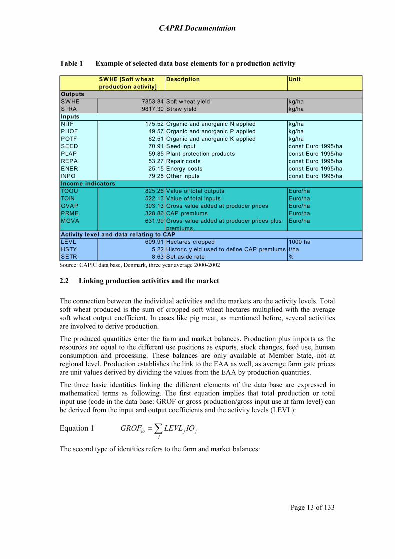
The main sources used to build up the national data base are shown in the following table and diagram.

Table 3 Data items and their main sources

Data items Source

Activity levels Land use statistics, herd size statistics, slaughtering statistics, statistics on import and export of live animals

Production Farm and market balance statistics, crop production statistics, slaughtering statistics, statistics on import and export of live animals

Farm and market balance positions

Farm and market balance statistics

Sectoral revenues and costs Economic Accounts for Agriculture (EAA)

Prices Derived from production and EAA

Output coefficients Derived from production and activity levels, engineering knowledge

Input coefficients Different type of estimators, engineering functions

Activity specific income indicators

Derived from input and output coefficients and prices

Policy data Various sources (Official Journal of the EU)

Source: Eurostat (http://epp.eurostat.cec.eu.int), several bio-physical econometric studies and European Commission (http://publications.eu.int/general/oj_en.html).

2.3.2 Estimation procedure

COCO was primarily designed to fill gaps or to correct inconsistencies found in statistical data and, additionally, to easily integrate data from non-EUROSTAT sources in the model. However, given the task of having to construct consistent time series on yields, market balances, EAA positions and prices for all EU Member States, a heavy weight was put on a transparent and uniform econometric solution so that manual corrections were avoided.

3 The ‘Common Agricultural Policy Simulation Model’ (CAPSIM) was developed by Dr. Heinz-Peter Witzke, EuroCare, Bonn (http://www.eurocare-bonn.de/profrec/capsim/capsim_e.htm).

CAPRI Documentation

of 133

COCO included data ranging from 1985 to 2002 for the 14 member states of the EU4 at that time, from the national data found in NEWCRONOS5. Regarding the construction of the data base, three principal problems had to be solved:

(1) Gaps had to be filled in time series, either before the first available point, inside the range where observations are given, or beyond it.

(2) Some time series were missing altogether and had to be estimated, e.g. when there are data on animal production but none on meat output per head.

(3) Minimal corrections of given statistical data, if not in line with the accounting identities, had to be made.

In order to take into account logical relation between the time series to fill, and eventually to make minimal corrections in the light of consistency definitions, simultaneous estimation techniques are used in this exercise. In order to use to the greatest extent the information contained in the existing data, the following principles are applied:

(1) Accounting identities. -positions of the market balance summing up to zero, the difference between stocks as the stock change and similar restrictions- constrain the estimation outcome.

(2) Relations between aggregated time series (e.g. total cereal area) and single time series are used as additional restrictions in the estimation process.

(3) Bounds for the estimated values based on engineering knowledge or derived from first and second moments of times series ensure plausible estimates and/or bind estimates to original data. Additionally, bounds are constructed from more disaggregated time series, if the aggregate is missing.

(4) As many time series as technically possible are estimated simultaneously to use the full extent of the informational content of the data constraints (1) and (2).

The first three points can be interpreted as a kind of ‘Bayesian’ approach: additional ‘a priori’ information supplements the estimation. However, in classical ‘Bayesian’ analysis, the information is expressed as a distribution of the parameters to estimate. For our purpose, such a concept would be complex and intransparent, as the fitted value and not the estimated parameter is of major interest. Further on, the statistical properties of the estimators are in our case of minor importance -we do not need good estimates of the parameters but consistent, plausible and good fitted values- leaving room for further ‘expert knowledge’ information.

The reader may notice that the problem is quite similar to system estimation in economics. Consider a system of supply curves. Given ex-post data, we naturally want the estimates to fit the given data as close as possible, but simultaneously require the estimates to be in line with economic theory. The latter point is typically ensured by two approaches: (1) the estimation equations are in line with some optimisation problem in the background (for example profit maximisation, i.e. the supplied outputs are regressed on a function of prices whose functional form is derived from first order conditions of a profit maximisation problem) and (2) appropriate restrictions on the parameters ensure that the resulting system is in line with

4 In CAPRI Luxembourg is aggregated to Belgium as a NUTS 2 region. The 10 new Member States were included in 2004. 5 Data for Norway are processed by COCO as well, but naturally, stem from different sources.

CAPRI Documentation

of 133

first and second order conditions of a profit maximisation problem. The ultimate aim is the combination of a functional form and parameter restrictions which allows for both a good fit and conformity with micro-economic theory.

Our approach is quite similar, as our goal asks for consistent estimates as well. But, there are two important differences, (1) we need to correct the original data as well -that would be the estimated values ex-post- and (2) it is very complex or simply impossible to define the full set of consistency conditions over restrictions on the estimated parameters in our case. Instead, we introduce explicit data constraints involving the fitted values for each point and take the fitted values later as the content of the data base.

The concept works in the following steps:

1. Estimate independent trend lines for the time series.

2. Estimate a Hodrick-Prescott filter using given data where available and otherwise the trend estimate as input.

3. Define ‘supports’ where are (a) given data, (b) the results from the Hodrick-Prescott

filter times R² plus the last (1-R²) times the last known point.

The concept is put to work by the minimisation of normalised least squares under constraints:

Equation 4

( )

( )

*,

,,,

,*,,

,,

,*,

,2

,

2,,

,

2,,

*,,,

)5.1(

)4.1(

)3.1(

)2.1(..

)(min)1.1(,

ti

utiti

lti

utiti

lti

titi

tititiiii

tititi

yiftitititicba

yondefinedidentitiesAccounting

eee

yyy

yifyynotify

eTcTbats

sdevresew

yyyti

iii

≤≤

≤≤⎩⎨⎧

=+++

+

−

∑

∑

where:

• a,b,c are the parameters to estimate and describe a polynomial trend fit, y are given and y* fitted values, e the error terms of the estimation, sdevres is the standard deviation of the errors of an unconstrained trend line and T trend.

• i represents the index of the elements to estimate (crop production activities or groups, herd sizes etc.), t stands for the year and the subscripts l and u are the indices for upper and lower bounds of the estimates and errors.

The objective function minimises the sum of two relative squared errors: (1) between corrected and given data, and (2) differences between trend forecasts and given res. fitted data. The normalisation for the errors (second term) is based on the standard deviation of the error of an unconstrained linear term line. The normalisation was necessary and helpful to reflect the fact that the means of the time series entering the estimation deviate considerably. The normalisation hence leads to minimisation of relative errors instead of absolute ones.

CAPRI Documentation

of 133

The fitted values y* at known points will only deviate from the given data if the accounting identities cannot be solved without corrections. In that case, normalised squared corrections drive the process, e.g. to determine which elements of the market balance to correct.

It should be noted that fitted value y* and errors e are defined at unknown points in constraint (1.2) over a polynomial trend fit up to degree two. The equation guarantees hence completeness in times. The degree of the resulting polynomial form may be less than indicated depending on the number of available observations. The error terms at unknown points are introduced to allow conformity between trend estimates and accounting identities. At known points, the equations define the error terms, as usual in regressions.

Upper and lower bounds restrict the estimation outcome as indicated in (1.3) and (1.4). For certain series and observations they reflect logical bounds -as non-negativeness or bounds taken from engineering knowledge. For the remaining cases they are constructed from mean and variance of the known points to avoid curious forecasts.

Equation (1.5) indicates that consistency restrictions are added to the fitting process. These restrictions are discussed in details below.

Readers familiar with the work of the CAPRI team in the last years may wonder why the authors are using a modified least squares estimator and not a Cross (CE) or Maximum Entropy Estimator (ME). The reasons are similar to the points mentioned above regarding the application of a ‘Bayesian’ approach: the ex-ante knowledge can be expressed mainly relating to the estimated value and not in relation to estimated parameters. Accordingly, supports would need to be defined at least for the error terms and the consistency slacks. The authors are convinced that the current framework can be mapped without greater problems in an entropy estimator, but expects a higher computational burden due to the more complex objective function.

2.3.3 Defining upper and lower bounds for the estimated value

The initial approach fixed observations at given data and did not include bounds for the trend estimates. Already first tests showed that the trend outcomes could look rather awkward, especially when several observations were missing at the ends of time series, and the necessity of bounds became obvious. If several elements of a market balance are missing, for instance, the consistency condition certainly influence the outcome of the process, but if to the better is not clear beforehand. In order to keep estimates in a plausible range, we defined an estimation corridor for missing observations based on a moving average and the variance of each time series.

Naturally, it became obvious immediately that not all given data could be fixed. Assume, for instance, that all elements for a balance are given, but the balance is not closed. Such a data constellation would yield infeasibilities. In order to allow for the necessary correction, a tight corridor around all given data values was introduced. As the approach was tested on a growing number of data sets, these tight bounds initially introduced around given data were more and more relaxed to accommodate for inconsistencies in the original data, and rules were introduced to widen them depending on data constellations. The code was growing larger and larger with rather complex if-else rules depending on possible inconsistencies in the given data to avoid infeasibilities. The envisaged transparency was in danger to be lost.

After a critical evaluation, the procedure was revised, based on the following arguments. Firstly, if corrections on original data are allowed even if these are already consistent, there may be a sizeable trade-off between a better trend fit for the missing data and corrections of the existing ones. The declared aim was however to correct original data only when necessary. Secondly, any update of the original data may provoke new inconsistencies, thus

CAPRI Documentation

of 133

asking for larger correction bounds, or the introduction or revision of rules to define these bounds.

Accordingly, the solution should be able to detect if and where original data provoke infeasibilities, and introduce solely corrections at these points. The dual solution from minimising the sum of infeasibilities from the estimation problem shown above is used to define optimal correction corridors. If the problem is infeasible with given bounds, the shadow values on (1.2) to (1.5) show which bounds or constraints provoke the infeasibilities. As consistency constraints cannot be dropped, a feasible solution can hence only be found if bounds are relaxed. Fortunately, the dual solution indicates exactly which bounds to correct. Exactly these bounds are stepwise relaxed until all infeasibilities are removed and the optimisation can start. The process first relaxes bounds for the estimates at missing points before bounds around given data are relaxed.

Fortunately, the process can be implemented quite easily. The gradient based solver CONOPT3 first searches for a feasible solution before working on the objective. If infeasibilities are found, shadow values on constraints and equations are reported based on estimated gradients from the minimisation of infeasibilities. It is hence not necessary to explicitly define the Lagrangian function of problem (1) in order to calculate the shadow values. The starting deviation allowed for given data is just 0.01% times the coefficient of variance of a linear trend on the time series, in order to avoid numerical problems with fixed variables.

The process has the advantage of self correction. If an update introduces a set of internally consistent data, the bounds from a former solution are not longer relevant, and the estimated values are fixed to the given ones. If an update provokes infeasibilities not found before, the process will automatically look up the minimal correction necessary to fulfil the consistency framework. Hence, chances are great that control costs for updates are small.

Naturally, the procedure may yield quite curious estimates for missing data if outliers are present and provoke pressure on estimates of missing data over the data constraints. The manifold checks on the results let us however conclude that such outliers are typically subject to rather large corrections themselves and do not have a sizeable impact on other series. The typical check is to plot the given data against the consistent ones for the key time series, and obvious outliers usually stick to the eye due to their high deviation against the original data. Discussions if and how an explicit statistical outlier test could and should be introduced in the framework are not yet finalised.

2.3.3.1 Bounds for trend estimates The process of defining and relaxing bounds is discussed based on an example. The original time series shown in red - "EL HCOM TOMA (Given)"- in the diagram below is rather typical for gaps in the raw data. Missing values can be found both in-between given points, and at the tails. The dark blue and turquoise series show the upper and lower bounds for the estimation corridor.

CAPRI Documentation

of 133

Figure 1. Example for bounds on trend estimates in CoCo

400

450500

550

600

650700

750

1 2 3 4 5 6 7 8 9 10 11 12 13 14 15 16 17

EL HCOM TOMA Given EL HCOM TOMA Estimy.LoEL HCOM TOMA Estimy.Up

Source: Own calculations

These lower and upper bounds are generated in the following way:

• In between the range of known points – here the points 1 to 14 - the estimation channel corresponds to +/- 0.05 standard deviation of the series from the next observed data point.

• For all other points – here the forecasted ones, 15 to 17 - the centre of the estimation channel is defined by the nearest known moving average plus 0.1 times the standard deviation of the time series.

2.3.3.2 The iterative procedure at work The lower and upper limits for the given points are replaced by very tight bounds for the given points before the solver is put to work, as seen in the next diagram, whereas the estimation corridor for the unknown points is unaffected. However, the combination of these bounds with the consistency constraints and all other bounds present simultaneously for other time series yielded infeasibilities in our example. Non-zero shadow values were found for three points (observations 13, 16 and 17). For observation 5 and 15, estimates are at lower bounds, but no shadow value was attached, so a correction of the bounds was not necessary.

CAPRI Documentation

of 133

Figure 2. Example for bounds on trend estimates in CoCo, continued

400

450500

550

600

650700

750

1 2 3 4 5 6 7 8 9 10 11 12 13 14 15 16 17

EL HCOM TOMA Estimy.Lo EL HCOM TOMA Estimy.UpEL HCOM TOMA Estimy.L


The third figure shows the estimation bounds and estimated values at the end of the optimisation stage when all infeasibilities had been removed and the objective function is at its optimum. It can be seen that the bounds had been relaxed for observations 13, 16 and 17. All the original values are (almost) fixed. The new points introduced certainly do not look like a trend fit, as they reflect the relation between consistency conditions, estimated gaps and given data in other time series. It should be noted that the lower bound on point 5 is active, probably pulling the estimated value from the trend line towards the neighbouring observations.

Figure 3. Example for bounds on trend estimates in CoCo, continued

400

450500

550

600

650700

750

1 2 3 4 5 6 7 8 9 10 11 12 13 14 15 16 17



CAPRI Documentation

of 133

400

450500

550

600

650700

750

1 2 3 4 5 6 7 8 9 10 11 12 13 14 15 16 17



2.3.4 Concluding remark on the estimation process

We may conclude that the process is a rather pragmatic one. Firstly, it certainly ensures that infeasibilities are avoided in most instances, thus reducing the control cost for a new data update. Secondly, the risk that original data are corrected without an inconsistency present is close to zero. Thirdly, the “sweeping tail” problem of trend estimates is to a certain extent reduced by introducing bounds.

The first trade-off is the use of an estimator with unknown large and small sample properties. Secondly, the process requires either a gradient based solver using a two-stage process searching first a feasible point or the Lagrangian of problem (1). Thirdly, the problem as defined above can only be solved by general NLP solvers, and is hence not easily portable to other software platforms as for instance a statistical package. And finally, the resulting solution can certainly not be easily “explained” as the chosen estimates and corrections are the outcome of a simultaneous optimisation problem.

Nevertheless, the teams involved are convinced that given their current resource endowment, the solution is as close to optimal as possible.

2.3.5 Data and estimation groups

The data entering the estimation process stem all from EUROSTAT collections. Physical production statistics and balance sheets are from the ZPA1 domain, prices from the PRAG domain and the EAA accounts stem from the COSA domain. Data are directly converted from the EUROSTAT formatted input files to GAMS tables without intermediate files via a home-written FORTRAN routine called DFTCON. The original EUROSTAT codes are converted to two dimensional item-product type codes, as far as possible already in CAPRI conventions.

The estimation is carried out independently for each member state. In order to reduce the computational burden and control costs, the process is subdivided additionally in the following parts:

(1) Estimation of hectares, yields and gross production for all crop products simultaneously.

CAPRI Documentation

of 133

(2) Estimation of farm and market balances for crop products, broken down in the following groups:

(2.1) Cereals

(2.2) Industrial crops including oilseeds

(2.3) Fruits

(2.4) Vegetables

(2.5) Wine

(2.6) Fodder from arable land

(2.7) A last group including all those time series which are not assigned to one of the above mentioned (e.g. sugar beets)

(3) Estimation of herd sizes, gross production output and farm and market balances for animal activities and products, broken down in the following groups:

(3.1) All activities and products related to the production and use of milk and sheep and goat meat

(3.2) Cattle group (fattening and raising activities, meat) without dairy cows (comprised in 3.1)

(3.3) Pigs

(3.4) Poultry

In the following sections the specific data constraints for the different estimation problems will be discussed in further detail.

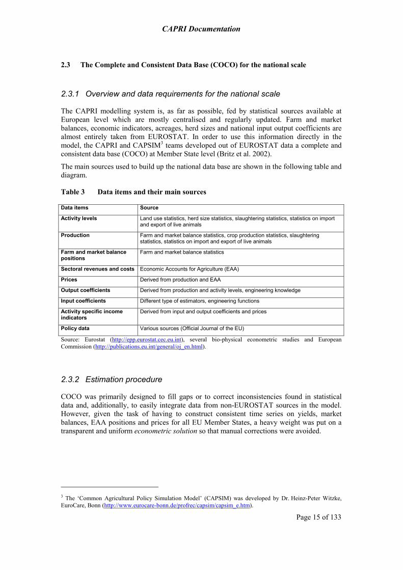
2.3.6 Consistent estimation of hectares, yields and gross production

Code: coco\coco_estimc.gms

Consistent estimation of hectares, yield and crop output gross production is the first of three separately defined estimation problems. The main outline of each of the estimation problems is defined above in problem (1). We will hence concentrate on the detailed description of the accounting identities restricting the estimation.

The simultaneous estimation of crop activity levels, yields and gross production is constrained by the following equations6:

Production of output equals activity level (hectares) multiplied with O-coefficients (Yields) (GrofD_)7

Equation 5 ∑=j

ijji OUTPLEVLGROF 001.0** ,

where: j denotes production activity

6 As far as possible we will use the codes and the units as documented in the data base. If not, they will be specified under the equation. Furthermore, we neglect the time and Member state index in the equation for better readability. However, it should be clear, that each consistency condition must hold in every year and for each Member state. 7 Name of equation in the code.

CAPRI Documentation

of 133

i denotes product GROF physical gross production (typically measured in 1000 t) LEVL activity level (measured in 1000 ha) OUTP Output coefficient (yield, typically in kg/ha)

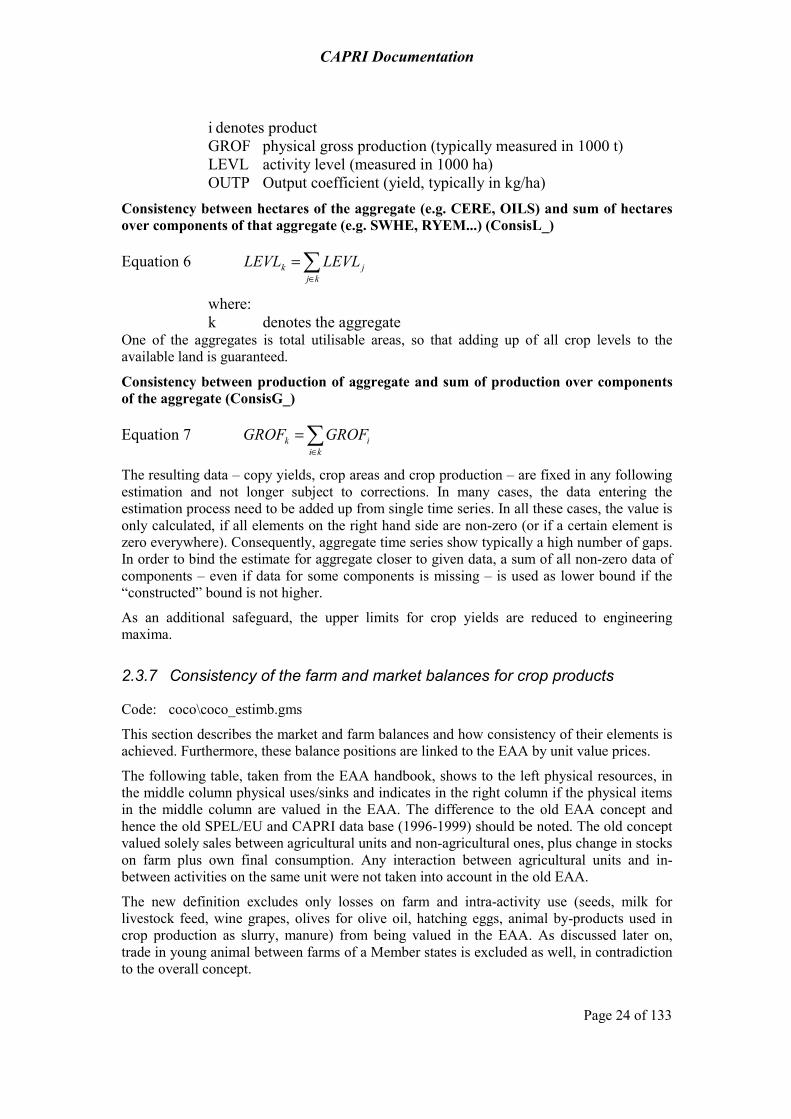
Consistency between hectares of the aggregate (e.g. CERE, OILS) and sum of hectares over components of that aggregate (e.g. SWHE, RYEM...) (ConsisL_)

Equation 6 ∑∈

=kj

jk LEVLLEVL

where: k denotes the aggregate

One of the aggregates is total utilisable areas, so that adding up of all crop levels to the available land is guaranteed.

Consistency between production of aggregate and sum of production over components of the aggregate (ConsisG_)

Equation 7 ∑∈

=ki

ik GROFGROF

The resulting data – copy yields, crop areas and crop production – are fixed in any following estimation and not longer subject to corrections. In many cases, the data entering the estimation process need to be added up from single time series. In all these cases, the value is only calculated, if all elements on the right hand side are non-zero (or if a certain element is zero everywhere). Consequently, aggregate time series show typically a high number of gaps. In order to bind the estimate for aggregate closer to given data, a sum of all non-zero data of components – even if data for some components is missing – is used as lower bound if the “constructed” bound is not higher.

As an additional safeguard, the upper limits for crop yields are reduced to engineering maxima.

2.3.7 Consistency of the farm and market balances for crop products

Code: coco\coco_estimb.gms

This section describes the market and farm balances and how consistency of their elements is achieved. Furthermore, these balance positions are linked to the EAA by unit value prices.

The following table, taken from the EAA handbook, shows to the left physical resources, in the middle column physical uses/sinks and indicates in the right column if the physical items in the middle column are valued in the EAA. The difference to the old EAA concept and hence the old SPEL/EU and CAPRI data base (1996-1999) should be noted. The old concept valued solely sales between agricultural units and non-agricultural ones, plus change in stocks on farm plus own final consumption. Any interaction between agricultural units and in-between activities on the same unit were not taken into account in the old EAA.

The new definition excludes only losses on farm and intra-activity use (seeds, milk for livestock feed, wine grapes, olives for olive oil, hatching eggs, animal by-products used in crop production as slurry, manure) from being valued in the EAA. As discussed later on, trade in young animal between farms of a Member states is excluded as well, in contradiction to the overall concept.

CAPRI Documentation

of 133

Table 4 EAA definition according to EUROSTAT

Resources

Uses Agricultural output of the agricultural

industry

Gross produc-

tion

Sales (total, excluding trade in animals between agricultural holdings)

X

Change in stocks (with producers) X -

Losses =

Own-account produced fixed capital goods (plantations, yielding repeat products, productive animals)

X

Own final consumption ( of agricultural products) X Usable output

Processing by producers (of agricultural products, separable)

X

Intra-unit consumption: for the same activity:(seeds, milk for livestock feed,

wine grapes, olives for olive oil, hatching eggs)

for a separate activity: • Crop products used in animal feed (cereals,

oilseeds, fodder crops, marketable or not, etc.) X

• Animal by products used in crop production (slurry, manure)

Source: EUROSTAT 2000, p. 42

The change introduced by the new definition of the EAA allowed for a simplification of the farm and market balances compared to the old CAPRI and SPEL/EU data base. The valued positions are now production minus losses, seed and internal use (manure, animal flows inside the sector), and a split up of stock changes, human consumption and feed between farm and market balance is not longer necessary.

2.3.7.1 Primary, non-processed products

Consistency of farm balance positions (ConsF_) “Farm” stands for the abstract national farm as the aggregate of all individual farms. The farm balance is built to mimic the valuation scheme of the EAA. In order to find the physical equivalent to the EAA “NETF”, losses on farm (LOSF), seed use on farm (SEDF) and internal use of animals and manure (INTF) deducted from gross production (GROF). All positions are in physical terms. Data for the farm positions are available in EUROSTAT for cereals, only. The INTF positions are zero for crops by definition.

Equation 8 iiiii NETFINTFLOSFSEDFGROF +++=

CAPRI Documentation

of 133

Consistency of market balance positions (ConsMkb_) The market balance is an accounting system which summarises transactions of all agricultural outputs on “markets”. Resources are transaction of the agricultural sector (NETF) or marketable production in case of secondary products (MAAR) plus total imports (IMPT) plus imports as live animals (IMPL) in case of meat.

Uses are exports (EXPT), seed use on market (SEDM), losses on market (LOSM), feed use (FEDM), industrial use (INDM), processing to secondary products (PRCM) and stock changes (STCM). Any statistical adjustments reported by EUROSTAT are set to zero. The reader is reminded that a distinction between seed and losses on farm and market is available for cereals, only.

Equation 9

iiii

iiiii

Meatiiondariesiprimariesi

SADMSTCMHCOMPRCMINDMFEDMLOSMSEDMEXPTIMPLIMPTMAPRNETF

++++++++=

++ ∈∈∈ sec

Consistency to Economic Accounts of Agriculture (ConsisEAA) The connection between the EAA valued position (EAAP: EAA value at producer prices) and the farm balance position “NETF” are unit values at producer prices (UVAP):

Equation 10 1000/* iii UVAPNETFEAAP =

It should be noted that the “NETF” position is derived from data in EUROSTAT’s ZPA1 domain. According to the new EAA handbook, member states are required to report both physical and valued data along with unit values prices in the EAA. One may hence question our decision to use ZPA1 data instead of the physical data from the EAA. First of all, not all member states report quantities and unit value prices. Secondly, differences between physical position NETF, derived from the farm and market balances, and the EAA physical values are sizeable in many cases. Using the EAA data would hence lead to inconsistencies between the farm and market balance positions. Nevertheless, we are left with the problem that the differences exist and are hard to interpret, and can lead to astonishing unit values, both regarding their level as their development over time, especially in a cross-country comparison. We hope that some of the differences can be clarified in future by contacts to EUROSTAT.

Consistency between farm and market balances positions for seed use and losses and total losses and seed use (ConsP_) The split up of positions in farm and market items exists solely for seeds and losses, the only positions where a split-up is necessary to accommodate the new EAA. As indicated above, seed and losses on farm are reported for cereals, only.

Equation 11 iii

iii

SEDMSEDFSEDTLOSMLOSFLOST

+=+=

Consistency between items of farm and market balance for aggregates and components (ConsisG_)

The conditions ensure as above for the crop production estimation group consistency between aggregate and member of the aggregate, for example that cereals imports are equal to the imports for soft wheat, barley ....

CAPRI Documentation

of 133

Equation 12 ∑∈

=ki

ik RESPOSRESPOS

where:

RESPOS comprises all positions relevant for farm and market balance (except prices and SADM)

2.3.7.2 The case for secondary products: There are a few secondary products – not valued by the EAA – comprised in the data base, namely oils and cakes from oilseeds, starch and rice. For these products, an explicit connection between processing of primaries and marketable production is established.

Processing relation: consistency between processing of primary products (PRCM) and marketable production (MAPR) of secondary ones (Process_)

Equation 13 ij

jij MAPRPRCYPRCM =∑ *

where:

PRCYji Processing yield, e.g. kg of soya oil extracted from one kg soya

Seed use is by definition not possible for secondary.

2.3.7.3 Consistency conditions for stock changes and stocks Modelling of stocks and stock changes is important for both, primary and secondary products.

Stock flow between the years (StocksLM_)

Equation 14 tititi STKMSTCMSTKM ,,1, =+−

where:

STKM Stock level

Limit sum of sum of stock changes over time to 10% of production (StocksAML_. StocksAMH_)

Equation 15

i,t i,ti,t

i,tt

i,t i,ti,t

i,tt

Mean("GROF ") Mean("IMPT ")STCM *0.1

Mean("MAPR ")

Mean("GROF ") Mean("IMPT ")STCM *0.1

Mean("MAPR ")

+⎡ ⎤< ⎢ ⎥+⎢ ⎥⎣ ⎦

+⎡ ⎤> − ⎢ ⎥+⎢ ⎥⎣ ⎦

∑

∑

The conditions are introduced to keep the estimator from “piling” up stocks over time.

CAPRI Documentation

of 133

2.3.8 Consistency of herd sizes, animal production and balance sheets8

As in the sections before, the aim of this part of the model is to construct a reliable data base regarding livestock activity levels and their respecting I/O coefficients in line with national statistics. In general, the layout of this estimation problem follows the same steps and uses partly the same equations as the two problems described beforehand.

Animal activity levels relate

(a) to an average of the countings in the current year (milk production, laying hens and sows) respectively an average of last year’s December counting, current year’s July/August counting and current year’s December counting (suckler and dairy cows) or

(b) to slaughtered plus exported minus imported heads (fattening activities: beef, heifers, male and female calves, pork, sheep and goat, poultry) or

(c) to young animals raised (male and female calves raising, heifers raising), measured in 1000 res. 1 million (laying hens and poultry fattening) heads.

The estimation problem is partly defined by means of the following already known equations from chapter 3:

(1) Production of output equals = activity level multiplied with O-coefficients (GrofD_)

(3) Consistency of production of aggregate to sum over production of the components (ConsisG_)

(4) Consistency of market balance positions (ConsMkb_)

(5) Consistency to Ecomomic Accounts of Agriculture (ConsisEAA_)

(7) Consistency of aggregate items of farm and market balance to sum over items of components (ConsisG_)

(8) Processing relation: consistency between resources of raw product and marketable production of processed ones (Process_)

(9) Consistency of market balance positions (ConsMkb_)

(10) Stock flow between the years (StocksLM_)

(11) Limit sum of stock changes to 10% of production (StocksAML_. StocksAMH_)

Besides these, the additional data consistency conditions formulated below constrain the estimation of herd sized, animal outputs and their balance sheets:

Definition of young animal input (IaniH_)

The need of each type of young animal is defined as follows:

Equation 16 IHEIiyLEVLHEIRIMPLEXPLSLGHGROF iyiyiyiy =∧+−+= .

where: SLGH slaughtered heads EXPL exported heads of live animals IMPL imported heads of live animals HEIR.LEVL number of heifers raised, only added if iy=IHEI

8 This section is mainly based on a draft written by Torbjörn Jansson and Anders Bäckstrand (SLI, Sweden).

CAPRI Documentation

of 133

Definition of meat output (IaniT_)

The meat output for each type of animal is defined as follows:

Equation 17 iyiyiyiyacctiyaact

meatacctaact IMPTEXPTSLGTIYANIOUTPLEVL −+=∑⇔

,,

where: aact iy animal activities using young animal category iy as

input OUTP Meat output coefficient YANI Young animal input coefficient SLGT slaughtered heads EXPT exported tons of live animals IMPL imported tons of live animals

The reader should note the difference to the data base. Here, the meat output is defined per slaughtered animal, where in the data base it is related to the activity level. Take dairy cows as an example: during estimation, the meat output coefficient relates to one cow slaughtered, and total meat output is the cow herd times the replacement rate times the carcass weight. In the data base, the meat output coefficient is per cow (= carcass weight times replacement rate).

Uses equal resources for young animals (YaniB_)

The balance equals resources of young animals (own production and import of live animals) with their use in fattening and raising activities. Stock changes are defined by the EAA as (des)investments and have to be booked by definition on the output side. Accordingly, there are never stock changes of young animals used as inputs. Furthermore, the EAA does not take into account sales of young animals from other farms or traders inside the country, nor interactions between animal activities of the same farm. Solely imports of live animals are valued by the EAA as costs in animal production. Accordingly, flows of all other young animals are by definition not valued by the EAA sector.

Each animal category features its own equation. Input and output of young animals are linked over a cross-set:

Equation 18 oyoyiy STCMGROFGROF −=

where: iy young animals as inputs (booked as costs) oy young animals as outputs (booked as revenues)

The equation states that gross need of young animals as inputs - typically equal number of slaughtered plus exported plus raised heads minus the imported heads is equal to the output of young animals minus stock changes. The distinction between young animals on the input and output side allows to calculate the intra-sectoral, intra-activity and intra-regional income effects of exchanges of young animals, which are consolidated by the EAA.

Consistency of number of imported calves (CalvesT_)

Imported calves are split up in male and female ones:

Equation 19 LEVLCAFFLEVLCAMFICALGROF ... +=

where: GROF.ICAL slaughtered plus exported minus imported calves

CAPRI Documentation

of 133

Fix relation between male and female young calves from dairy and suckler cows (MalFem1_), (MalFem2_)

The proportion of male calves in total calves born per dairy and per suckler cow is kept between 50 and 52%.

Equation 20 50.0*)(52.0*)(

cowscowsCows

cowscowsCows

YCAFYCAMYCAMYCAFYCAMYCAM

+≥+≤

Definition of stock changes for young animals (StocksA_)

a) For the animal categories where young animals are used in the same year (chicken, lambs, piglets)

Equation 21 ttt STCMLEVLLEVL =−+1

b) for heifers and bulls, it is the change in the raising activities of the last year (old animals outputted in the current year t stem from young ones produced in the year before t-1)

Equation 22 ttt STCMLEVLLEVL =− −1

c) for young cows, it is the change in the heifers raising activities plus stock change of dairy and suckler cows

Equation 23

t

tt

tt

tt

STCMLEVLSCOWLEVLSCOWLEVLDCOWLEVLDCOW

LEVLHEIRLEVLHEIR

=−+−+

−

+

+

−

....

..

1

1

1

Definition of protein and fat balance for milk processing on processing industry level (MLKCNT_)

Equation 24 iMLKSECOi

i MLKCNTMAPRMLKCNTMILKPRCM **. ∑∈

=

where: PRCM.MILK milk collected by dairies (cow and sheep/goat) MLKSECO set of elements which contain all secondary

commodities produced from milk (butter, cheese...)

MLKCNT table with protein and fat content of the different products

Consistency of EAA value of milk (EAAMLK_)

In the EAA, milk covers both cow and sheep/goat milk. A distinction is made between cow milk and milk from sheep and goat in the data base:

Equation 25 SGMIEAAPCOMIEAAPMILKEAAP ... +=

CAPRI Documentation

of 133

2.4 The Regionalised Data Base (CAPREG)

2.4.1 Data requirements at regional level

CAPRI aims at building up a Policy Information System of the EU’s agricultural sector, regionalised at NUTS 2 level with an emphasis on the impact of the CAP. The core of the system consists of a regionalized agricultural sector model using an activity based non-linear programming approach. One feature of such a highly disaggregated, activity based agricultural sector model is the detailed information resulting from ex-ante simulations of policy scenarios concerning the output and input of specific agricultural production activities and their relationships. This information is also a pre-condition to judge possible impacts of agricultural production on the environment. However, these systems require as well this kind of information (data) ex-post, at least partially. It is especially necessary to define for each region in the model, at least for the basis year, the matrix of I/O-coefficients for the different production activities together with prices for these outputs and inputs. Moreover, for calibration and validation purposes information concerning land use and livestock numbers is necessary.

Given the importance of the EU as an international player on agricultural world markets, neither world nor EU market prices can be treated as exogenous to the model. Therefore, a market module links the supply side of the model with national and international markets for agricultural products. For the time being, the smallest market region in the CAPRI is the Member State level, thought to be a spot market for all regional units intern of the Member State. This simplification allows to use national data to cover the model’s market side.

2.4.2 Data sources at regional level

Already during the first CAPRI meeting, the REGIO domain of EUROSTAT was judged as the only harmonized data source available on regionalized agricultural data in the EU. REGIO is one of several parts of NEWCRONOS and is itself broken down in domains, one of which covers agricultural and forestry statistics.

In the agricultural and forestry domain [AGRI] the following tables are available:

• Land use [A2LAND]

• Crop production - harvested areas, production and yields [A2CROPS]

• Animal production - livestock numbers [A2ANIMAL]

• Cows’s milk collection - deliveries to dairies, % fat content [A2MILK]

• Agricultural accounts on regional level [A2ACCT]

• Structure of agricultural holdings [A2STRUC, A3STRUC]

• Labour force of agricultural holdings [A2WORK]

2.4.3 Data availability at regional level

The following table shows the official availability of the different tables of REGIO. However, the current coverage concerning time and sub-regions differs dramatically between the tables and within the tables between the Member States.

CAPRI Documentation

of 133

A second problem consists in the relatively high aggregation level especially in the field of crop production. Hence, additional sources, assumptions and econometric procedures must be applied to close data gaps and to break down aggregated data.

Table 5 Official data availability in REGIO

Table Official availability

Land use from 1974 yearly

Crop production (harvested areas, production and yields)

from 1975 yearly

Animal production (livestock numbers) from 1977 yearly

Cows’s milk collection (deliveries to dairies, % fat content)

from 1977 yearly

Agricultural accounts on regional level from 1980 yearly

Structure of agricultural holdings 1983, 1985, 1987, 1989/91, 1993

Labour force of agricultural holdings from 1983 yearly

Source: Eurostat (http://epp.eurostat.cec.eu.int)

2.4.4 Reading and storing the original REGIO data

The original REGIO data are stored in an ASCII-format designed by EUROSTAT for NEWCRONOS and used in connection with the CUB-X, EUROSTAT’s data browser. The data can be browsed and extracted to several formats directly with CUB-X (one table each time). However, in the case of the CAPRI-project, data from several tables must be merged together, adding up to some million numbers. CUB-X was never designed for such quantities. Therefore, the group in Bonn designed a tool called DFTCON which converts these files into a rather simple format:

− In a first step, these files are sorted by region, year and original code, so that they can be easily accessed by other software to perform extraction from the original NEWCRONOS data base.

− In a second step these files are read, the original codes are assigned to eight character strings and the resulting table per region and year is stored in binary compressed form in the data base.

The result of these two steps are tables, one for each regional unit available at NUTS 0 to NUTS 2 level in REGIO and each year which comprise all data from the REGIO tables: land use, crop production, animal populations, cow’s milk collection and agricultural accounts. These tables are stored in a data management system designed for use in agricultural sector modelling.

2.4.5 Methodological proceeding

The starting point of the methodological approach is the decision to use the consistent and complete national data base (COCO) as a frame or reference point for any regionalization. In other words, any aggregation of the main data items (areas, herd sizes, gross production and intermediate use, unit value prices and EAA-positions) of the regionalized data over regions must match the national values.

CAPRI Documentation

of 133

Given that starting position, the following approaches are generally applied:

• Data enter the consistency checks as found in REGIO. This is mainly true for animal herd sizes where REGIO offers data at the same or even more disaggregated level as found in COCO.

• Gaps in REGIO are filled out and data found in REGIO at a higher aggregation level as required in CAPRI are broken down by using existing national information.

• Functions used are structurally and (often) numerically identical for all regional units and groups of activities and inputs/outputs.

• Econometric analysis or additional data sources are used to close gaps.

All the approaches described in the following sub-sections are only thought as a first crude estimate. Wherever additional data sources are available, their content should be checked and made available to overcome the list of these ‘easy-to-use’ estimates presented in here. The procedures described in here can be thought as a ‘safety net’ to ensure that regionalized data are technically available but not as an adequate substitute for collecting these data from additional sources.

2.4.6 Prices for outputs and inputs

Code: capreg\price_yani.gms

The agricultural domain of REGIO does not cover regionalized prices. For simplicity, the regional prices are therefore assumed to be identical to sectoral ones9:

Equation 26 sr UVAGUVAG =

Young animal prices are a special case since they are not included in the COCO data base (the current methodology of the EAA does not value intermediate use of animals) but are necessary to calculate income indicators for intermediate activities (e.g. raising calves). Only exported or imported live animals are implicitly accounted for by valuing the connected meat imports and exports.

Young animals are valued based on the ‘meat value’ and assumed relationships between live and carcass weights. Male calves (ICAM, YCAM) are assumed to have a final weight of 55 kg, of which 60 % are valued at veal prices. Female calves (ICAF, YCAF) are assumed to have a final weight of 60 kg, of which 60 % are valued at veal prices. Young heifers (IHEI, YHEI) are assumed to have a final weight of 300 kg, of which 54 % are valued at beef. Young bulls (IBUL, YBUL) are assumed to have a final weight of 335 kg, of which 54 % are valued at beef. Young cows (ICOW, YCOW) are assumed to have a final weight of 575 kg, of which 54 % are valued at beef. For piglets (IPIG, YPIG), price notations were regressed on pig meat prices and are assumed to have a final weight of 20 kg of which 78 % are valued at pig meat prices. Lambs (ILAM, YLAM) are assumed to weight 4 kg and are valued at 80 % of sheep and goat meat prices. Chicken (ICHI, YCHI) are assumed to weight 0.1 kg and are valued at 80 % of poultry prices.

2.4.7 Filling gaps in REGIO

Code: capreg\trend.gms 9 There is no easy way to relax this assumption if no further data sources are available.

CAPRI Documentation

of 133

In cases where data in REGIO on regional level are missing, a linear trend line is estimated for the Member State time series in REGIO definition. The average relation between regional and national data where both are available is then multiplied with the national trend value to derive a trend estimate at regional level.

2.4.8 Mapping crop areas and herd sizes from REGIO to COCO definitions

Code: capreg\map_from_regio.gms

Only some few crop activities are available in REGIO (cereals with wheat, barley, grain maize, rice; potatoes, sugar beet, oil seeds with rape and sunflower; tobacco, fodder maize; grassland, permanent crops with vineyards and olive plantations). The COCO data base, however, covers some 30 different crop activities. In order to break these aggregates down to COCO definitions, the national shares of the aggregate are used.

As an example, this approach is explained for cereals. Data on the production activities BARL (barley), MAIZ (grain maize) and PARI (paddy rice) as found in COCO match directly the level of disaggregation in REGIO. Therefore, the regionalized data are directly set to the values in REGIO. The difference between the sum of these 3 activities and the aggregate data on cereals in REGIO must be equal to the sum of the remaining activities in cereals as shown in COCO, namely RYE (rye and meslin), OATS (oats) and OCER (other cereals). As long as no other regional information is available, the difference from REGIO is broken down applying national shares.

The approach is shown for OATS in the following equations, where the suffix r stands for regional data:

Equation 27

r r rOATS,COCO

r rOATS,r

OATS,COCO RYE,COCO OCER,COCO

CEREAL WHEAT BARLEYLEVL

MAIZEGR RICELEVL

LEVL LEVL LEVL

− −⎛ ⎞⎜ ⎟− −⎝ ⎠=

+ +

Similar equations are used to break down other aggregates and residual areas in REGIO10.

One important advantage of the approach is the fact that the resulting areas are automatically consistent to the national data if the ingoing information from REGIO was consistent to national level. Fortunately, the regional information on herd sizes covers most of the data needed to give nice proxies for all animal activities in COCO definition. REGIOs break down for herd sizes is more detailed than COCO -at least for the important sectors. Regional estimates for the activity levels are therefore the result of an aggregation approach, in opposite to crop production.

2.4.9 Perfect aggregation between regional and national data for activity levels

Besides technological plausibility and a good match with existing regional statistics, the regionalized data for the CAPRI model must be also consistent to the national level. The minimum requirement for this consistency includes activity levels and gross production.

Consistency for activity levels is momentarily achieved by first using the approaches described above to produce first estimates (Levlr) for the relevant data items and then by calculating and applying in a second step correction factors. 10 If no data at all are found, the share on the utilisable agricultural area is used.

CAPRI Documentation

of 133

Equation 28 LEVLjrjrj

njr

rjLEVLj

CORRLevlLevl

LevlLevlCORR

,,*,

,,,

*=

= ∑

Code: capreg\cons_levls.gms

A specific problem is the fact that land use statistics do not report a break down of idling land into obligatory set-aside, voluntary set-aside and fallow land11. Equally, the share of oilseeds grown as energy crops on set-aside needs to be determined.

An entropy estimator is used to ‘distribute’ the national information on the different types of idling land to regional level, with the following restrictions

• Obligatory set-aside areas must be equal to the set-aside obligations derived from areas and set-aside rates for Grandes Cultures (which may differ at regional level according to the share of small producers). For these crops, activity levels are partially endogenous in the estimation in order to allow a split up of oilseeds into those grown under the set-aside obligations and those grown as non-food crops on set-aside.

• Obligatory and voluntary set-aside cannot exceed certain shares of crops subjects to set-aside (at least before Agenda 2000 policy)

• Fallow land must equalise the sum of obligatory set-aside, voluntary set-aside and other idling land.

• Total utilisable area must stay constant.

In some cases, areas reported as fallow land are smaller than set-aside obligations. In these cases, parts of grassland areas and ‘other crops’ are allowed to be reduced.

The proceeding for gross output (GROF) is similar to the one for activity levels, as correction factors are applied to line up regional yields with given national production:

Equation 29 oGROFrjrj

nojr

rjrjoGROF

CORROO

GROFOLevlCORR

.,*,

,,

,,,

*=

=∑

In case of missing statistical information for regional yields, national yields are used. A special rule is used for fodder maize yields, where regional yields are derived from national fodder maize yields, and the relation between regional and national average cereal yields. For grassland and fodder from arable land, missing yields are derived from national ones using the relation between regional and national stocking densities of ruminants. The stocking densities are calculated by multiplying herd sizes with live stock units and dividing the resulting sum of livestock units by the grassland, fodder maize and other fodder on arable land areas.

Code: capreg\cons_yields.gms

11 The necessary additional information on non-food production on set-aside, obligatory and voluntary set-aside areas can be found on the DG-AGRI web server.

CAPRI Documentation

of 133

2.4.10 Estimating expected yields with a Hodrick-Prescott filter

The input allocation in any given year should not be linked to realised, but to expected yields. Expected yields are constructed using the following modified Hodrick-Prescott filter:

Equation 30 ( ) ( )∑∑ −+−=−<<

−+t

ttTt

tt yyyyhp 2*

11

2*1

*11000min

where y covers all output coefficients in the data base. The Hodrick-Prescott filter is applied both at the national and regional level after any gaps in the time series had been closed.

2.5 The world Data Base

The global data base of CAPRI comprehends macro-economic data for different world regions, policy data and global agricultural production data. Several data sources can be mentioned:

• Data on bilateral trade between selected world regional aggregates (main trading players) are borrowed from the World Agricultural Trade Simulation Model (WATSIM).

• Data on policy variables such as applied and scheduled tariffs, tariff rate quotas or bilateral trade agreements are obtained from the AGLINK Model (OECD) and the Agricultural Market Access Database (AMAD).

• Preferences. Changes in demand behaviour not linked to income or prices changes are trended using ex post time series on per capita consumption, in most cases in line with data found in the EU Prospects for Agricultural Markets (European Commission).

• The price framework contained in the market module is based on representative long term time series for world market prices of major raw and processed agricultural product, which are trend forecasted.

These data are necessary for the construction of a world trade model (comprehending certain world regional aggregates), which should deliver some price feedback to the European supply system.

CAPRI Documentation

of 133

3 Input Allocation

The term input allocation describes how aggregate input demand (e.g. total anorganic N fertiliser use in Denmark) is ‘distributed’ to production activities. The resulting activity specific data are called input coefficients. They may either be measured in value (€/ha) or physical terms (kg/ha). The CAPRI data base uses physical terms and, where not available, input coefficient measured in constant prices.

Micro-economic theory of a profit maximising producer requires revenue exhaustion, i.e. marginal revenues must be equal to marginal costs simultaneously for all realised activities. The marginal physical input demand multiplied with the input price exhausts marginal revenues, leading to zero marginal profits. Marginal input demands per activity can only be used to define aggregate input demand if they are equal to average input demands. The latter is the case for the Leontief production function.

The advantage of assuming a Leontief technology in agricultural production analysis is the fact that an explicit link between production activities and total physical input use is introduced (e.g. environmental indicators can be linked directly to individual activities or activity specific income indicators, since gross margins can be calculated). The disadvantage is the rather rigid technology assumption. We would for example expect that increasing a crop share in a region will change the average soil quality the crop uses, which in turn should change yields and nutrient requirements. It should hence be understood that the Leontief assumption is an abstraction and simplification of the ‘real’ agricultural technology in a region. The assumption is somewhat relaxed in CAPRI as two ‘production intensities’ are introduced.

Input coefficients for different inputs are constructed in different ways which will be discussed in more detail in the following sections:

• For nitrate, phosphate and potash, nutrient balances are constructed so to take into account crop and manure nutrient content and observed fertiliser use, combined with a simple fixed coefficient approach for ammonia losses. These balances ex-post determine the effective input coefficients based on a cross-entropy estimation framework.

• For feed, the input calculation is rooted in a mix of engineering knowledge (requirement functions for animal activities, nutrient content of feeding stuff), observed data ex-post (total national feed use, national feed costs) and estimated feed costs from a FADN sample, combined within a Highest Posterior Density (HPD) estimation framework.

• For the remaining inputs, estimation results from a FADN sample are combined with aggregate national input demand reported in the EAA and standard gross margin estimations, again using a HPD estimation framework.

3.1 Input allocation excluding young animals, fertiliser and feed

3.1.1 Background

There is a long history of allocating inputs to production activities in agricultural sector analysis, dating back to the days where I/O models and aggregate farm LPs where the only quantitative instruments available. In these models, the input coefficients represented a

CAPRI Documentation

of 133

Leontief technology, which was put to work in the quantitative tools as well. However, input coefficients per activity do not necessary imply a Leontief technology. The allocated input demands can be seen as marginal ones (which are identical to average ones in the Leontief case) and are then compatible with flexible technologies as well.

Input coefficients can be put to work in a number of interesting fields. First of all, activity specific income indicators may be derived, which may facilitate analyzing results and may be used in turn to define sectoral income. Similarly, important environmental indicators are linked to input use and can hence be linked to activities as well with the help of input coefficients.

Given the importance or the input allocation, the CAP-STRAT project (2000-2003) comprised an own work package to estimate input coefficients. On a first step, input coefficients were estimated using standard econometrics from single farm record as found in FADN. Additionally, tests for a more complex estimation framework building upon entropy techniques and integrating restrictions derived from cost minimization were run in parallel.

The need to accommodate the estimation results with data from the EAA in order to ensure mutual compatibility between income indicators and input demand per activity and region on the one hand, and sectoral income indicators as well as sectoral input use on the other, requires deviating from the estimated mean of the coefficients estimated from single farm records. Further on, in some cases estimates revealed zero or negative input coefficients, which cannot be taken over. Accordingly, it was decided to set up a second stage estimation framework building upon the unrestricted estimates from FADN. The framework can be applied to years where no FADN data are available, and thus ensures that the results will be continuously used for the years ahead, before an update of the labor-intensive estimations is again necessary and feasible.

3.1.2 Econometric Estimation

Standard econometric methods were employed to calculate input coefficients from single farm records found in FADN (within a consistent aggregation framework, as explained in chapter 6). Raw data were transformed into CAPRI compatible categories. Fixed-Effects, Random Effects, Weighted Fixed-Effects, and Weighted Random-Effects as well as OLS and WLS models were tested with varying degrees of success. After finding heteroskedasticity problems, deciding to neglect from using an intercept (in order to conform to the Leontief technology assumed by the model) and after comparing results for plausibility, it was decided that a straightforward WLS model was the most suitable form if a consistent estimation technique was to be used for all estimations. The main reason for choosing such a simple WLS estimator over a weighted random effects model with no ‘fixed effect’ intercept was the question of plausibility of results. Specification tests suggested, in fact, that fixed effects estimators might have been used in every regression, but apart from the problem of distributing farm specific fixed effect intercepts across crop and animal activities, there were two (related) reasons not to use these results. Firstly, the results of the fixed effects specifications –on the whole- were implausible, with a large number of negative coefficients. Secondly, it was felt that any possible endogeneity in the estimations would probably have a greater proportionate effect in the fixed effects results. The weight actually used in the final WLS versions was total output.

Initial experiments also revealed a high degree of multicollinearity if activity levels and outputs were both used on the right hand side. Accordingly, it was decided to use output on the right hand side if possible (so that regional variations could be incorporated into the model). Where sufficient output values were not available, activity levels were used, using the criterion described below. Furthermore, because of a clearly deleterious effect on results,

CAPRI Documentation

of 133

the equivalents of the CAPRI residual activity categories OCRO (other crops), OFRU (other fruits), OCER (other cereals), OVEG (other vegetables), etc. were all dropped from the estimations.

All regressions were run using STATA 7.0. Price indices were taken from the COCO database in order to calculate input costs in real terms. The starting sample sizes were, as follows, all multiplied by 10 (for the years 1990-1999) unless otherwise stated:

•AT - Austria - 2451 farms

•BL - Belgium, 2601 farms

•DE - Germany, 15110 farms --> price data from ‘91-’99

•DK - Denmark, 6625 farms

•EL - Greece, 11877 farms --> price data from ’95-’99

•FI - Finland, 1324 farms

•IR - Ireland, 3409 farms --> no price data prior to 1995

•IT - Italy, 57264 farms

•PT - Portugal, 6379 farms

•SE - Sweden, 1191 farms

•UK - United Kingdom, 6668 farms

•ES - Spain, 22609 farms

•NL – Netherlands, 3565 farms

•FR – France, 17332 farms

The following data cleaning procedures were used:

− The regressors with less than or equal to 100 observations for both activity levels and output were excluded.

− The data were truncated at zero in order to eliminate reported negative level and output values and also reported negative real input costs.

− All non-zero values were counted and a choice made between either activity level or output, as the appropriate right-hand side variable (only one could be use to avoid multicollinearity).

− An activity’s output value was used if the number of non-zero output values associated with that activity was greater than the number of the activity’s non-zero levels minus 500. Thus, output was always the preferred option unless levels were reported for at least 500 more observations than outputs. This procedure was necessary because of a number of cases in the data when only output or activity level values but not both.

Several regressions were run to yield estimates for coefficients in each of 11 input categories: Total Inputs, Crop Only Inputs, Animal Only Inputs, Seeds, Plant Protection, Fertilizer, Other Crop Inputs, Purchased and Non-Purchased Feeds and Other Animal Only Inputs.

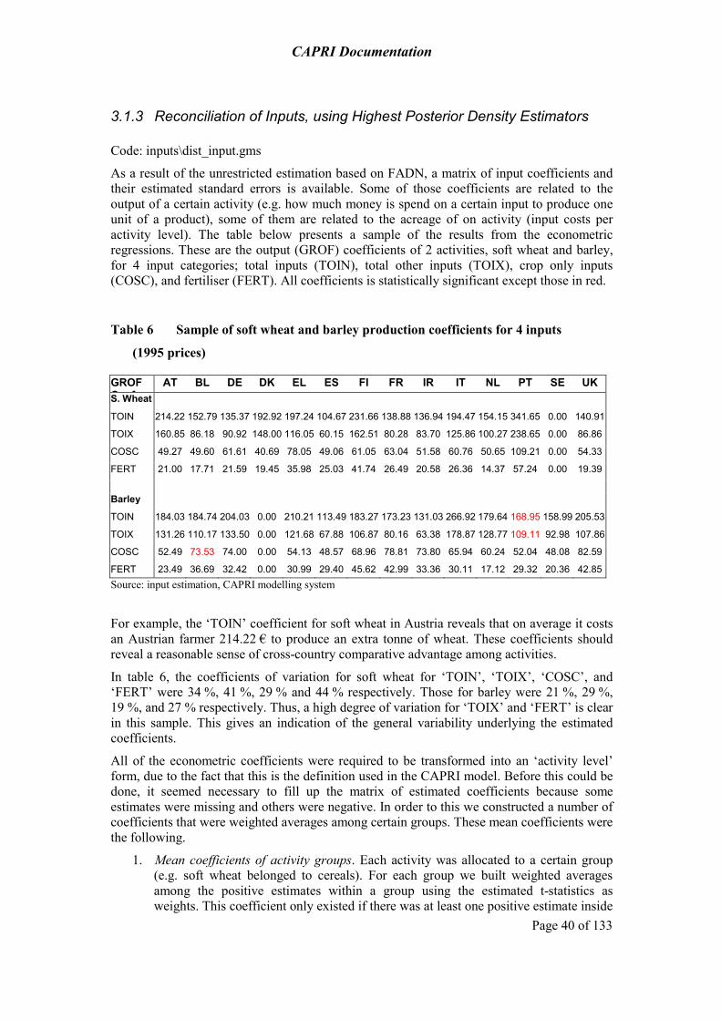
CAPRI Documentation

of 133

3.1.3 Reconciliation of Inputs, using Highest Posterior Density Estimators

Code: inputs\dist_input.gms

As a result of the unrestricted estimation based on FADN, a matrix of input coefficients and their estimated standard errors is available. Some of those coefficients are related to the output of a certain activity (e.g. how much money is spend on a certain input to produce one unit of a product), some of them are related to the acreage of on activity (input costs per activity level). The table below presents a sample of the results from the econometric regressions. These are the output (GROF) coefficients of 2 activities, soft wheat and barley, for 4 input categories; total inputs (TOIN), total other inputs (TOIX), crop only inputs (COSC), and fertiliser (FERT). All coefficients is statistically significant except those in red.

Table 6 Sample of soft wheat and barley production coefficients for 4 inputs

(1995 prices)

GROF C f

AT BL DE DK EL ES FI FR IR IT NL PT SE UK S. Wheat

TOIN 214.22 152.79 135.37 192.92 197.24 104.67 231.66 138.88 136.94 194.47 154.15 341.65 0.00 140.91

TOIX 160.85 86.18 90.92 148.00 116.05 60.15 162.51 80.28 83.70 125.86 100.27 238.65 0.00 86.86

COSC 49.27 49.60 61.61 40.69 78.05 49.06 61.05 63.04 51.58 60.76 50.65 109.21 0.00 54.33

FERT 21.00 17.71 21.59 19.45 35.98 25.03 41.74 26.49 20.58 26.36 14.37 57.24 0.00 19.39

Barley

TOIN 184.03 184.74 204.03 0.00 210.21 113.49 183.27 173.23 131.03 266.92 179.64 168.95 158.99 205.53

TOIX 131.26 110.17 133.50 0.00 121.68 67.88 106.87 80.16 63.38 178.87 128.77 109.11 92.98 107.86

COSC 52.49 73.53 74.00 0.00 54.13 48.57 68.96 78.81 73.80 65.94 60.24 52.04 48.08 82.59

FERT 23.49 36.69 32.42 0.00 30.99 29.40 45.62 42.99 33.36 30.11 17.12 29.32 20.36 42.85 Source: input estimation, CAPRI modelling system

For example, the ‘TOIN’ coefficient for soft wheat in Austria reveals that on average it costs an Austrian farmer 214.22 € to produce an extra tonne of wheat. These coefficients should reveal a reasonable sense of cross-country comparative advantage among activities.

In table 6, the coefficients of variation for soft wheat for ‘TOIN’, ‘TOIX’, ‘COSC’, and ‘FERT’ were 34 %, 41 %, 29 % and 44 % respectively. Those for barley were 21 %, 29 %, 19 %, and 27 % respectively. Thus, a high degree of variation for ‘TOIX’ and ‘FERT’ is clear in this sample. This gives an indication of the general variability underlying the estimated coefficients.

All of the econometric coefficients were required to be transformed into an ‘activity level’ form, due to the fact that this is the definition used in the CAPRI model. Before this could be done, it seemed necessary to fill up the matrix of estimated coefficients because some estimates were missing and others were negative. In order to this we constructed a number of coefficients that were weighted averages among certain groups. These mean coefficients were the following.

1. Mean coefficients of activity groups. Each activity was allocated to a certain group (e.g. soft wheat belonged to cereals). For each group we built weighted averages among the positive estimates within a group using the estimated t-statistics as weights. This coefficient only existed if there was at least one positive estimate inside

CAPRI Documentation

of 133

that group and was then used to replace the gaps inside the coefficient matrix. If that mean coefficient was not available, due to no positive estimate inside a group at all, the next type of mean coefficients became relevant:

2. Mean coefficients for an activity among European regions. This second type of mean coefficients calculates weighted averages among three types of regional clusters. These clusters are Northern European States, Southern European states and all European regions. Again, the estimated t-statistics were used as aggregation weights. Unfortunately, this type of averages did not fill all gaps in the coefficient matrix as there were some activities that had no positive estimate over the entire EU. For those the third type of mean coefficients was calculated.

3. Mean coefficients for activity groups among regional clusters. Here we calculated for the three regional clusters the averages of the first type of mean coefficients. As even the latter are synthetic, we gave each mean of them the same weight. Fortunately there was only a small probability that this coefficient did not exist for one of the groups as this was only the case if no coefficient inside a group over the entire EU had a positive estimate, which was not the case.

Following these rules we finally got a matrix of estimated and synthetic calculated input coefficients for both, the ‘per activity level’ and the ‘per production’ unit definition.12 For the synthetic one there was no estimated standard error available but we wanted to use those later on. So we assumed them –to reflect that these coefficients have only weak foundation– to have a t-statistic of 0.5.

The ‘per level’ definition was only taken over if the coefficient was really estimated or if no per production unit definition did exist. To transfer the latter into per activity level definition, we multiplied them with the average yield (1985-2001) of the respective activity. The resulting coefficients and their standard errors were then used in the cross entropy approach described below. 13

Missing econometric estimates and compatibility with EAA figures were not the only reasons that made a reconciliation of estimated inputs coefficients necessary. Moreover, the economic sense of the estimates could not be guaranteed and the definition of inputs in the estimation differed from the one used in CAPRI. Therefore we decided to include further prior information on input coefficients in agriculture. The second set of priors in the input reconciliation was therefore based on data from the EAA. Total costs of a certain input within an activity in a European Member State was calculated by multiplying the total expenditures on that input with the proportion of the total expected revenue of that activity to that of all activities using the input. Total expected revenue in this case was the production value (including market value and premiums) of the respective activity. If this resulted in a certain coefficient being calculated as zero due to missing data, then this coefficient would be replaced by one from a similar activity e.g. a zero coefficient for ‘MAIF’ would be replaced by the coefficient for ‘GRAS’

12 In addition, a similar procedure (using slightly different groups) was applied to constructing coefficients for the ‘Other’ activities (e.g. OCER, OFRU, OVEG), which had been omitted from the econometric estimations. They are given the average group coefficient, unless there is none; then they are given the average northern or southern European coefficient as appropriate. 13 Adjustments were made for scaling issues with regard to eggs for certain countries, and grass for Finland. In addition, when ‘CAFR’,’CAFF’ and ‘HEIR’ did not have econometric data, they assumed the coefficients and standard errors of ‘CAMR’, ‘CAMF’ and ‘HEIF’ respectively (CAPRI activity code definitions in table 29 or the appendix).

CAPRI Documentation

of 133

This kind of prior information tries to give the results a kind of economic sense. For the same reason the third type of priors was created based on standard gross margins for agricultural activities received from EUROSTAT. Those existed for nearly all activities. The set from 1994 was used, since this was the most complete available. Relative rather than absolute differences were important, given the requirement to conform to EAA values.14

3.1.4 Highest Posterior Density estimation framework

Given the three types of prior information explained above –estimated input coefficients, data from EAA and standard gross margins-, the choice of a HPD Estimator to reconcile estimated input coefficients seemed to be convenient.15 The estimation was carried out for all CAPRI activities (z) -excluding activities that where split up like DCOW into DCOL and DCOH-, and a number of inputs in CAPRI (denoted by XCI,z) and FADN (XFI,z) definition. The list of input definitions can be found in the annex (table 31).

For each prior we defined 4 support points (k) centred on the value of the priors defined as above. The support range was defined as follows:

• For the econometric estimates:

SXFi,z,k PXFi,z + [-100; -1; 1; 100] σXFi,z,

where SXF,I,z,k gives the support points for the FADN input XFI,z that has a standard error of σXFi.

• For the EAA priors: prior *(1+ [-10; -0.1; 0.1; 10]).

SXCi,z,k PXCi,z (1+ [-10; -0.1; 0.1; 10]),

where SXCi,z,k gives the support points for the CAPRI input XCI,z. A special treatment was chosen for the total input coefficient. Here the support range was half that from above.

• For the standard gross margins:

SGM,z,k PGM,z (1+ [-10; -0.1; 0.1; 10]),

where SXCi,k gives the support points for the standard gross margin of activity z.

We define the a priori probability for each support point to be:

APk = [0.002; 0.49; 0.49; 0.002],

in order to give the outermost support points less weight. Posterior probabilities are denoted by PP. The model setup is then given by:

14 Contrary to the econometric estimated priors, the two other types were different in different years, since the reconciliation had to be done for each year in the database. The second prior type is year specific by nature, as the EAA values differ between years. In case of standard gross margins, unfortunately, we had them only for one year (1994). So we decided to ‘drive them over time’ using the proportion of expected revenue of an activity in a certain year to that in the year 1994. 15 The advantage of cross entropy is that one can define the support space rather wide and give the edges a very low prior probability.

CAPRI Documentation

of 133

Equation 31

CI,Z,K FI,Z,K GM,Z,K

CI,Z,K FI,Z,KCI,Z,K FI,Z,K

K K

CI,FI,Z,K FI,Z,KGM,Z,K

K

CI,Z,K FI,Z,K GM,Z,Kk k k

CI

max H(PP ,PP ,PP )

PP PPPP ln PP ln

AP AP

PPPP ln

AP

s.t.PP 1, PP 1, PP 1

X

=

⎛ ⎞⎡ ⎤⎡ ⎤ ⎛ ⎞+⎜ ⎟⎢ ⎥⎜ ⎟⎢ ⎥

⎜ ⎟⎣ ⎦ ⎝ ⎠⎢ ⎥−⎜ ⎟⎢ ⎥⎛ ⎞⎜ ⎟⎢ ⎥+ ⎜ ⎟⎜ ⎟⎢ ⎥⎝ ⎠⎣ ⎦⎝ ⎠

= = =

∑

∑ ∑ ∑

,Z CI,Z,K CI,Z,K FI,Z FI,Z,K FI,Z,Kk k

Z GM,Z,K GM,Z,Kk

Z Z CI,Z exo,ZCI G1(CI,Z)

CI CI,Z ZZ G1(CI,Z)

CI,Z FI,ZCI G2(CI,FI)

FI,Z CI,ZFI G3(CI,FI)

FI1,Z FI,FI1 G4(FI,FI1)

PP S , X PP S

GM PP S

GM EREV X X

EAA X LEVL

X X

X X

X X

∈

∈

∈

∈

∈

= =

=

= − −

=

=

=

=

∑ ∑

∑

∑

∑

∑

∑

∑ Z

The first two rows of the equation shown above are subject to maximize cross entropy, while the third row guaranties that all probabilities sum up to unity. In the fourth row, the estimates for input coefficients and gross margins are re-parameterized from the posterior probabilities and the support points. The fifth row defines gross margins for an activity z as the difference between expected revenue per activity level (EREV) of that activity and the sum over all inputs used in that activity. The Set G1(CI,Z) allocates the inputs used to each activity and Xexo,Z are inputs, that are not estimated here, but cannot be neglected in defining gross margins (like young animal inputs). In the sixth row, we find a statement which guarantees that the sum over all activities of their activity levels multiplied with an input gives the total expenditures on that Input given by the EAA. The seventh and eighth rows link the inputs in the CAPRI definition to those in FADN definition. The first of those two are used when the FADN inputs are an aggregate of CAPRI inputs (defined in the set G2(CI,FI)) or they have the same definition and the second one when CAPRI inputs are an aggregate of FADN inputs. Since estimated inputs in the FADN definition exist for aggregates and components of them, we ensure in the last line that the sum over FADN inputs that belong to an aggregated FADN input (defined in the set G4(FI,FI1)) sum up to the latter.

The estimation is carried out in GAMS within and run for each year in the database. Some bounds are further set to avoid estimates running into implausible ranges.

3.1.5 How are the results used in CAPRI?

The cross entropy estimation yields monetary input coefficients for the fertiliser types (Nitrate, Phosphate, Potassium), seeds, plant protection, feeds, pharmaceutical inputs, repairs,

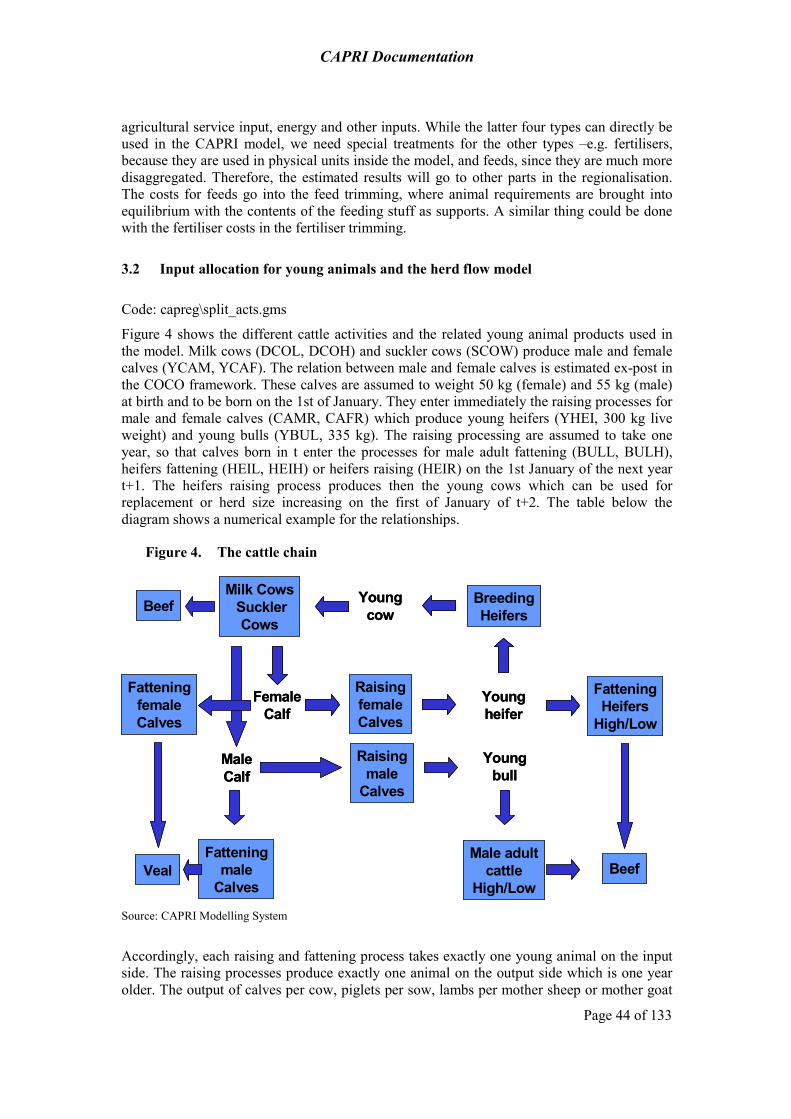
CAPRI Documentation

of 133

agricultural service input, energy and other inputs. While the latter four types can directly be used in the CAPRI model, we need special treatments for the other types –e.g. fertilisers, because they are used in physical units inside the model, and feeds, since they are much more disaggregated. Therefore, the estimated results will go to other parts in the regionalisation. The costs for feeds go into the feed trimming, where animal requirements are brought into equilibrium with the contents of the feeding stuff as supports. A similar thing could be done with the fertiliser costs in the fertiliser trimming.

3.2 Input allocation for young animals and the herd flow model

Code: capreg\split_acts.gms

Figure 4 shows the different cattle activities and the related young animal products used in the model. Milk cows (DCOL, DCOH) and suckler cows (SCOW) produce male and female calves (YCAM, YCAF). The relation between male and female calves is estimated ex-post in the COCO framework. These calves are assumed to weight 50 kg (female) and 55 kg (male) at birth and to be born on the 1st of January. They enter immediately the raising processes for male and female calves (CAMR, CAFR) which produce young heifers (YHEI, 300 kg live weight) and young bulls (YBUL, 335 kg). The raising processing are assumed to take one year, so that calves born in t enter the processes for male adult fattening (BULL, BULH), heifers fattening (HEIL, HEIH) or heifers raising (HEIR) on the 1st January of the next year t+1. The heifers raising process produces then the young cows which can be used for replacement or herd size increasing on the first of January of t+2. The table below the diagram shows a numerical example for the relationships.

Figure 4. The cattle chain

Beef

Beef

Veal Beef

Beef

Veal

RaisingfemaleCalves

Fatteningmale

Calves

BreedingHeifers

Milk CowsSucklerCows

Male adultcattle

High/Low

FatteningHeifers

High/Low

FatteningfemaleCalves

Raisingmale

Calves

RaisingfemaleCalves

Fatteningmale

Calves

BreedingHeifers

Milk CowsSucklerCows

Male adultcattle

High/Low

FatteningHeifers

High/Low

FatteningfemaleCalves

Raisingmale

Calves

MaleCalf

Youngheifer

Youngbull

Youngcow

FemaleCalf

MaleCalf

Youngheifer

Youngbull

Youngcow

FemaleCalf

Source: CAPRI Modelling System

Accordingly, each raising and fattening process takes exactly one young animal on the input side. The raising processes produce exactly one animal on the output side which is one year older. The output of calves per cow, piglets per sow, lambs per mother sheep or mother goat

CAPRI Documentation

of 133

is derived ex post, e.g. simultaneously from the number of cows in t-1, the number of slaughtered bulls and heifers and replaced in t+1 which determine the level of the raising processes in t and number of slaughtered calves in t. The herd flow models for pig, sheep and goat and poultry are similar, but less complex, as all interactions happen in the same year, and no specific raising processes are introduced.

Table 7 Example for the relation inside the cattle chain (Denmark, 1999-2001)

1999 2000 2001Male calves used in t and born in tDCOWLEVL Number of dairy cows 667.03 654.08 631.92DCOWYCAM Number of male calves born per 1000 dairy cows 420.72 438.62 438.26Number of males calves born from dairy cows 280.63 286.89 276.95SCOWLEVL Number of suckler cows 127.36 126.91 124.85SCOWYCAM Number of male calves born per 1000 suckler cows 420.72 411.83 401.61Number of male calves born from suckler cows 53.58 52.27 50.14Number of all male calves born 334.22 339.16 327.09GROFYCAM Number of male calves produced 334.21 339.16 327.09CAMFLEVL Number of male calves fattened 81.32 72.57 49.18CAMRLEVL Activity level of the male calves raising process 252.89 266.59 277.91Sum of processes using male calves 334.21 339.16 327.09GROFYCAM Number of male calves used 334.21 339.16 327.09Female calves used in t and born in tDCOWLEVL Number of dairy cows 667.03 654.08 631.92DCOWYCAF Number of female calves born per 1000 dairy cows 404.15 421.58 412.86Number of female calves born from dairy cows 269.58 275.75 260.89SCOWLEVL Number of suckler cows 127.36 126.91 124.85SCOWYCAF Number of male calves born per 1000 suckler cows 404.15 398.04 387.21Number of female calves born from suckler cows 51.47 50.52 48.34Number of all female calves born 321.05 326.26 309.24GROFYCAF Number of female calves produced 321.05 326.27 309.24CAFFLEVL Number of female calves fattened 26.64 28.74 18.39CAFRLEVL Activity level of the female calves raising process 294.41 297.53 290.85Female calves used in t and born in t 321.05 326.27 309.24GROFYCAF Number of female calves used 321.05 326.27 309.24Young bulls used in t and young bulls produced in tBULFLEVL Activity level of the bull fattening process 262.94 252.89 266.59GROFIBUL Number of young bulls used 262.94 252.89 266.59GROFYBUL Number of young bulls raised from calvs 252.89 266.59 277.91CAMRLEVL Activity level of the male calves raising process 252.89 266.59 277.91Heifers used in t and heifers produced in tHEIFLEVL Activity level of the heifers fattening process 64.36 67.25 68.12HEIRLEVL Activity level of the heifers raising process 235.45 227.16 229.4Sum of heifer processes 299.81 294.41 297.52GROFIHEI Number of heifers used 299.81 294.41 297.53GROFYHEI Number of heifers raised from calves 294.41 297.53 290.85CAFRLEVL Activity level of the female calves raising process 294.41 297.53 290.85Cows used in t and heifers produced in tDCOWLEVL Number of dairy cows 667.03 654.08 631.92DCOWICOW Number of young cows needed per 1000 dairy cows 332.01 332.5 327.52Sum of young cows needed for the dairy cow herd 221.46 217.48 206.97DCOWSLGH Slaugthered dairy cows 221.47 217.48 206.11SCOWLEVL Number of suckler cows 127.36 126.91 124.85SCOWICOW Number of young cows needed per 1000 suckler cows 332.01 332.48 327.52Sum of young cows needed for the suckler cow herd 42.28 42.20 40.89SCOWSLGH Slaugthered suckler cows 42.29 42.19 40.72Sum of slaughtered cows 263.76 259.67 246.83GROFICOW Number of young cows used 263.75 259.67 247.86Stock change in dairy cows (DCOWLEVL(t+1)-DCOWLEVL(t) -12.95 -22.16Stock change in suckler cows (SCOWLEVL(t+1)-SCOWLEVL(t) -0.45 -2.06Sum of stock changes in cows -13.4 -24.22Sum of slaughtered cows and stock change 235.45GROFYCOW Numer of heifers raised to young cows 235.45 227.16 229.4HEIRLEVL Activity level of the heifers raising process 235.45 227.16 229.4 The table above is taken from the COCO data base. In some cases, regional statistical data or estimates for number of young animals per adult are available, but in most cases, all input and output coefficients relating to young animals are identical at regional and national level. Nevertheless, experiences with simulations during the first CAPRI project phase revealed that a fixed relationship between meat output and young animal need as expressed with on bull

CAPRI Documentation

of 133

fattening process overestimates the rigidity of the technology in the cattle chain, where producers may react with changes in final weights to relative changes in output prices (meat) in relation to input prices (feed, young animals). A higher price for young animals will tend to increase final weights, as feed has become comparatively cheaper and vice-versa. In order to introduce more flexibility in the system, the dairy cow, heifer and bull fattening processes are split up each in two processed as shown in the following table.

Table 8 Split up of cattle chain processes in different intensities

Low intensity/final weight High intensity/final weight

Dairy cows (DCOW) DCOL: 60% milk yield of average, variable inputs besides feed an young animals at 60% of average

DCOH: 140% milk yield of average, variable inputs besides feed an young animals at 140% of average

Bull fattening (BULF) BULL: 20% lower meat output, variable inputs besides feed an young animals at 80% of average

BULH: 20% higher meat output, variable inputs besides feed an young animals at 120% of average

Heifers fattening (HEIF) HEIL: 20% lower meat output, variable inputs besides feed an young animals at 80% of average

HEIH: 20% higher meat output, variable inputs besides feed an young animals at 120% of average

3.3 Input allocation for feed

The input allocation for feed describes how much kg of certain feed categories (cereals, rich protein, rich energy, feed based on dairy products, other feed) or single feeding stuff (fodder maize, grass, fodder from arable land, straw, milk for feeding) are used per animal activity level16.

The input allocation for feed takes into account nutrient requirements of animals, building upon requirement functions. The input coefficients for feeding stuff shall hence ensure that energy, protein requirements, etc. cover the nutrient needs of the animals. Further on, ex-post, they should be in line with regional fodder production and total feed demand statistics at national level, the latter stemming from market balances. And last but not least, the input coefficients together with feed prices should lead to reasonable feed cost for the activities.

3.3.1 Estimation of fodder prices

Since the last revision of the EAA, own produced fodder (grass, silage etc.) is valued in the EAA. Individual estimates are given for fodder maize and fodder root crops, but no break down is given for fodder on arable land and fodder produced as grassland as presented in the CAPRI data base. The difference between grass and arable land is introduced, as conversion of grass to arable land is forbidden under cross-compliance conditions so that marginal values of grassland and arable land may be different.

16 The reader should notice again that the activity definition for fattening processes are slaughtered plus exported minus imported animals and not stable places.

CAPRI Documentation

of 133

The price attached to fodder should reflect both its nutritional content and the production costs at regional level. The entropy based estimation process tries to integrate both aspects.

The following equations are integrated in the estimator. Firstly, the regional prices for ‘grass’, ‘fodder on arable land’ and ‘straw’ (fint) multiplied with the fed quantities at regional level must exhaust the vale reported in the economic accounts, so that the EAA revenues attached to fodder are kept unchanged:

Equation 32 ∑ +=fint,

,,fint,fint,r

MSGRASMSOFARrr EAAPEAAPPFODFEDUSE

Secondly, the Gross Value Added of the fodder activities is defined as the difference between revenues and total input costs based on the input allocation for crops described above

Equation 33 fint,fint,fint,fint, rrrr TOINPFODYIELDGVAM −=

Next, the standard ingredients of a cross entropy estimator are added: definition of the estimated values from supports and the posterior probabilities, summing up of the posterior probabilities to unity and the definition of the cross entropy itself

Equation 34

∑

∑

∑

∑

∑

∑

−

−=

=

=

=

=

kpricerkkgvamrkgvamr

kpricerkkpricerkpricer

kkpricer

kkgvamr

rkpricerk

kpricer

rkgvamrk

kgvamr

pqpp

pqppPROBH

p

p

PFODp

GVAMp

,,fint,,,fint,,,fint,

,,fint,,,fint,,,fint,

,,fint,

,,fint,

fint,,,fint,,,fint,

fint,,,fint,,,fint,

)log(

)log()(

1

1

sup

sup

The a priori mean for the prices of ‘grass’ and ‘other fodder on arable land’ are the EAAP values divided by total production volume which is by definition equal to feed use. The price of straw for feed use is expected to be at 1 % of the grass price. The outer supports are set so that the higher support is at four times the a priori mean.

Supports for Gross Value Added per activity are centred around 150 % of the value of total inputs as allocated by the rules and algorithm described above, with rather wide bounds. The a priori probabilities for the three supports are set at 1 %, 98 % and 1 %.

The wide supports for the Gross Value Added of the fodder activities mirror the problem of finding good internal prices but also the dubious data quality both of fodder output as reported in statistics and the value attached to it in the EAA. The wide supports allow for negative Gross Value Added, which may certainly occur in certain years depending on realised yields. In order to exclude such estimation outcomes as far as possible an additional constraint is introduced:

Equation 35 gvafacTOINPFODYIELD rrr fint,fint,fint, ≥

The parameter gvafac is initialised with unity so that first a solution is tried where all activities have revenues exceed costs. If infeasibilities arise, the factor is stepwise reduced

CAPRI Documentation

of 133

until feasibility is achieved, to ensure that the minimal number of activities with negative Gross Value Addeds is estimated.

3.3.2 Feed input coefficients Feed use determines to a large extent costs of animal production as well as the use of certain crops as for fodder or cereals, and of secondary products as oilseeds as by-products of the milling industry. Hence, from the view point of policy modelling, a plausible description of the relations between animal production, feed use and market prices for feeds is necessary.

The issue has been addressed by a broad range of methodological solutions in sector models. Some important solutions are characterised as follows:

(1) Products used for feed are modelled as net-puts, only, depending on crop and animal prices and further factors, e.g. technological progress and availability of primary factors. Hence, the net-put approach models (intra-sectoral) feed use implicitly. Typically, the relevant parameters are estimated based on duality in the context of a profit function where the production possibility set is hidden. Plausibility checks of these hidden technological relations are hard to do and still harder to incorporate in the estimation approach.

(2) Feed use is modelled explicitly, but the underlying technology is hidden, e.g. when cost functions for the feed compound industry are estimated as in BRITZ & SIEBER (1998). Modelling feed use as a function of prices is quite common, for example in multi-commodity models such as WATSIM of the IAP or the World Food Model of the FAO. The technological relations are hidden as in (1), but somewhat easier to check by comparing the change in animal production provoked by a price change with its effects on feed use.

The next solutions refer to programming models:

(3) Feed use is modelled as fix cost per unit of animal production activities. Animal production will not be affected directly by changes in crop production and vice versa, but only indirectly by an update of the fix cost coefficients.

(4) Feed use is modelled via feeding activities. In that case, the model typically simultaneously determines the optimal levels of animal and crop production and the amount of each output fed to the animals. These solutions differ by:

a) The aggregation level of the feeding stuff. Some models, for example the German sector model RAUMIS, have feeding activities for each output to each animal activity, excluding technological impossible combinations such as feeding straw to piglets. The solution typically leads to a rather high number of feeding activities. Others, as the SPEL-MFSS, use aggregates of raw products in the feeding activities. Last but not least, single raw products can be mixed to different predefined menus whose mix is then the endogenous variable, as in TASM.

b) The definition of the constraints. In RAUMIS and SPEL-MFSS (WEBER 1995, pp. 39), requirements such as energy or protein are modelled explicitly. If mixes for certain animals are defined beforehand, explicit requirement constraints in the model may be left out if each individual mix guarantees already that requirements are covered. The higher the number of feed use activities per animal activity, and the lower the number of requirement constraints, the higher the chance of strongly overspecialised solutions. In order to ensure a "plausible" mix of the feeding activities, bounds on the feeding activities are sometimes used, as in SPEL-MFSS

CAPRI Documentation

of 133

or in earlier versions of RAUMIS. The substitution possibilities may be influenced by using PMP on feeding activities, as in the new version of RAUMIS (CYPRIS 1999).

Solution (3) and (4) may be iteratively coupled to modules which determine the costs for solution (3) or prices used in solution (4).

3.3.2.1 Solution in CAPRI Such an iterative coupling is the case in CAPRI which addresses the question of modelling the relations between animal and crop production, price and markets as follows:

• Feed use of non-tradable fodder such as grazing is modelled by individual feeding activities in the regional supply models. Whereas feeding activities of tradable products such as wheat or soya beans are aggregated to five categories (cereals, rich protein, rich energy, milk based and others).

• Requirement constraints (energy, protein, lysine etc.) are introduced to ensure technological plausible substitution between feeds.

• Calibration to an estimated feed input allocation ex-post is guaranteed by PMP calibration terms. The estimated feed input allocation guarantees that the feed positions of the national market balances are met, and that resulting feed costs are plausible.

• Tradable feeding stuffs can be sold and bought in unlimited quantities. No difference is made between tradable feeding stuffs produced in the region and such bought (net trade approach).

• Gras, fodder maize, other fodder from arable land and straw are assumed to be tradable only inside a regional unit. All quantities produced in the regions must be fed to regions or can be lost, the latter however only in the case of straw.

• The regional models are solved independently from each other with prices for outputs and inputs - including feeding stuff - fixed.

• Regional net trade from the regional supply model is aggregated per Member State and enters the behavioural functions of the market module including the quantities of the five feed aggregates. The link between the regional supply modules and the market modules is described in more detail below.

• Market module and regional supply models are iteratively linked where prices from the market module are used in the supply module generating quantities that in turn are used in the market module. For the five feed aggregates, the market module determines - with each iteration a new price and new nutrient contents for the feed aggregates (for details see: HECKELEI, BRITZ & LOEHE 1998).

The subsequent sections are mostly devoted to the question how the regional models embedded in the specific CAPRI layout described above can be specified in a way that

calibration of observed feeding quantities is achieved, and

a plausible simulation behaviour for feed use is obtained. An important feature of the CAPRI model is a rather explicit, primal modelling of feeding activities in the supply part as a cost minimising problem. Substitution possibilities in feeding

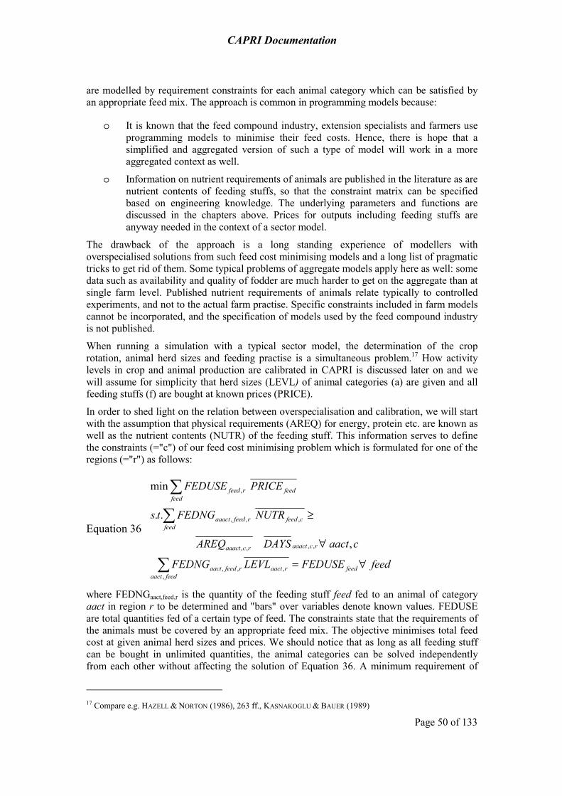
CAPRI Documentation

of 133

are modelled by requirement constraints for each animal category which can be satisfied by an appropriate feed mix. The approach is common in programming models because:

o It is known that the feed compound industry, extension specialists and farmers use programming models to minimise their feed costs. Hence, there is hope that a simplified and aggregated version of such a type of model will work in a more aggregated context as well.

o Information on nutrient requirements of animals are published in the literature as are nutrient contents of feeding stuffs, so that the constraint matrix can be specified based on engineering knowledge. The underlying parameters and functions are discussed in the chapters above. Prices for outputs including feeding stuffs are anyway needed in the context of a sector model.

The drawback of the approach is a long standing experience of modellers with overspecialised solutions from such feed cost minimising models and a long list of pragmatic tricks to get rid of them. Some typical problems of aggregate models apply here as well: some data such as availability and quality of fodder are much harder to get on the aggregate than at single farm level. Published nutrient requirements of animals relate typically to controlled experiments, and not to the actual farm practise. Specific constraints included in farm models cannot be incorporated, and the specification of models used by the feed compound industry is not published.

When running a simulation with a typical sector model, the determination of the crop rotation, animal herd sizes and feeding practise is a simultaneous problem.17 How activity levels in crop and animal production are calibrated in CAPRI is discussed later on and we will assume for simplicity that herd sizes (LEVL) of animal categories (a) are given and all feeding stuffs (f) are bought at known prices (PRICE).

In order to shed light on the relation between overspecialisation and calibration, we will start with the assumption that physical requirements (AREQ) for energy, protein etc. are known as well as the nutrient contents (NUTR) of the feeding stuff. This information serves to define the constraints (="c") of our feed cost minimising problem which is formulated for one of the regions (="r") as follows:

Equation 36

feedFEDUSELEVLFEDNG

caactDAYSAREQ

NUTRFEDNGts

PRICEFEDUSE

feedraactfeedaact

rfeedaact

rcaaactrcaaact

feedcfeedrfeedaaact

feedfeedrfeed

∀=

∀

≥

∑

∑

∑

,,

,,

,,,,

,,,

,

,

..

min

where FEDNGaact,feed,r is the quantity of the feeding stuff feed fed to an animal of category aact in region r to be determined and "bars" over variables denote known values. FEDUSE are total quantities fed of a certain type of feed. The constraints state that the requirements of the animals must be covered by an appropriate feed mix. The objective minimises total feed cost at given animal herd sizes and prices. We should notice that as long as all feeding stuff can be bought in unlimited quantities, the animal categories can be solved independently from each other without affecting the solution of Equation 36. A minimum requirement of

17 Compare e.g. HAZELL & NORTON (1986), 263 ff., KASNAKOGLU & BAUER (1989)

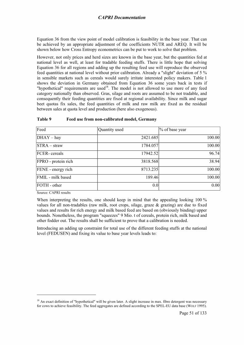
CAPRI Documentation

of 133

Equation 36 from the view point of model calibration is feasibility in the base year. That can be achieved by an appropriate adjustment of the coefficients NUTR and AREQ. It will be shown below how Cross Entropy econometrics can be put to work to solve that problem.

However, not only prices and herd sizes are known in the base year, but the quantities fed at national level as well, at least for tradable feeding stuffs. There is little hope that solving Equation 36 for all regions and adding up the resulting feed use will reproduce the observed feed quantities at national level without prior calibration. Already a "slight" deviation of 5 % in sensible markets such as cereals would surely irritate interested policy makers. Table 1 shows the deviation in Germany obtained from Equation 36 some years back in tests if "hypothetical" requirements are used18. The model is not allowed to use more of any feed category nationally than observed. Gras, silage and roots are assumed to be not tradable, and consequently their feeding quantities are fixed at regional availability. Since milk and sugar beet quotas fix sales, the feed quantities of milk and raw milk are fixed as the residual between sales at quota level and production (here also exogenous).

Table 9 Feed use from non-calibrated model, Germany

Feed Quantity used % of base year

DHAY – hay 2421.685 100.00

STRA – straw 1784.057 100.00

FCER- cereals 17942.52 96.74

FPRO - protein rich 3818.568 38.94

FENE - energy rich 8713.235 100.00

FMIL - milk based 189.46 100.00

FOTH - other 0.0 0.00 Source: CAPRI results

When interpreting the results, one should keep in mind that the appealing looking 100 % values for all non-tradables (raw milk, root crops, silage, graze & grazing) are due to fixed values and results for rich energy and milk based feed are based on (obviously binding) upper bounds. Nonetheless, the program "squeezes" 9 Mio. t of cereals, protein rich, milk based and other fodder out. The results shall be sufficient to prove that a calibration is needed.

Introducing an adding up constraint for total use of the different feeding stuffs at the national level (FEDUSEN) and fixing its value to base year levels leads to:

18 An exact definition of "hypothetical" will be given later. A slight increase in max. fibre detergent was necessary for cows to achieve feasibility. The feed aggregates are defined according to the SPEL-EU data base (WOLF 1995).

CAPRI Documentation

of 133

Equation 37

feedFEDUSENFEDUSE

feedFEDUSELEVLFEDNG

caactDAYSAREQ

NUTRFEDNGts

PRICEFEDUSE

feedrfeed

rfeed

feedraactfeedaact

rfeedaact

rcaaactrcaaact

feedcfeedrfeedaaact

feedfeedrfeed

∀=

∀=

∀

≥

∑

∑

∑

∑

,,

,,

,,

,,,,

,,,

,

,

..

min

The last line ensures that the known quantities fed at national level are met. Unfortunately, Equation 36 is not longer a cost minimisation problem, because quantities to be fed at national level and their prices are known! Consequently, the value of the objective function in Equation 37,

Equation 38 ∑∑ =feed

feedfeedrfeed

feedrfeed PRICEFEDUSENPRICEFEDUSE,

,

is a given constant. If we plug the problem shown above in a solver, it cannot squeeze out any quantities since total use is fixed at national level. It will simply distribute the feed over regions and animals so that the requirements of animals are met. When the first feasible solution for the requirement constraints is found, it will stop. The distribution will be arbitrary, with potentially devastating consequences for the feed costs of the regional activities. Naturally, some of the constraints in Equation 36 will be binding, but which ones will be arbitrary as well (as will be the dual values attributed to them).

Readers familiar with the on-going discussion on Positive Mathematical Programming (PMP) will now tend to lay back and relax because they know already a nice solution to the calibration problem. Their obvious idea will be to use the dual values on the variables FEDUSEN to define additional non-linear terms to be added to the objective function19. Naturally, perfect calibration will be guaranteed by the PMP methodology. But what about the simulation behaviour?

If the model without calibration bounds produces a solution dramatically different from the observed one (see Table 9), the influence of the PMP terms for feed on the simulation behaviour will be tremendous. Consequently, the effect of the requirement constraints will be small, hard to judge and depend on the quite arbitrary solution from the calibration step. The goal to describe the substitution possibilities in feeding by an appropriate set of constraints would surely be missed. Perhaps the best advice with such a solution would be to leave them out completely.

Instead, appropriate own and cross-cost terms between feeding activities would need to be introduced to describe the cost minimising behaviour in feeding. The technological substitution possibilities between feeding stuffs which we aimed at describing by the constraints in Equation 37 would be mostly hidden as dual information in these cost terms.

But there are further problems related to a PMP approach. Since the most expensive feeding stuff will always be squeezed out first, dual values of the corresponding calibration constraints will be equal to exogenous prices. Cross-regional or time series analysis of the duals from a sample of regional models will hence not produce any additional information.

19 PMP for feed are used, for example, in the RAUMIS model (CYPRIS 1999).

CAPRI Documentation

of 133

Without observed variance, a reliable estimation is not possible. The - at first sight - appealing PMP solution will consequently not work well, if no further information is available.

The essence of the argumentation above is that the use of an aggregated cost minimisation model in simulation runs is only sensible, if the constraints based on the coefficients (NUTR and REQU) can sufficiently explain observed feed use in the base year. Therefore, the "hypothetical" requirements must first be calibrated with respect to observed feeding quantities in the base year. Then, as a last resort, PMP can be put to work.

The general problem is then to define a set of requirements which calibrates the feed cost LP as close as possible to statistically observed quantities. It is solved by the following steps.

(STEP 1.) Definition of nutritional content (NUTR) of feeding stuffs. Whereas for cereals and other traded feeding stuffs, the information about their content of energy, protein etc. is quite accurate, doubt may be raised concerning fodder (gras, grazings, hay, silage etc.), both related to yield estimates and nutritional content. These contents are hence treated as endogenous variable in the estimation problem.

(STEP 2.) Definition of nutritional requirements (AREQ) for each animal category in each region based on so-called requirement functions as described above. For certain animal categories, additional requirements or constraints are introduced (lysine, max. dry matter intake, neutral detergent fibre etc.). For some of the animal categories they reflect differences in regional yields per head, for example the milk yield per cow. The underlying functions are based on a literature search and can be understood as the technological frontier under a controlled experimental environment.

(STEP 3.) Calibration of these hypothetical requirements and constraints so that they are as far as possible binding for the observed feed quantities. The necessity of calibrating the theoretical requirements can be easily understood when taking into account the control cost on farm level related to work exactly on the technological frontier: the nutrient content of feeding stuffs must be carefully checked and the intake of each feed per animal exactly weighted. Otherwise, one risks to starve the animal, to damage their health and to reduce yields, with high costs involved. To exclude that risk, farmers will feed securely more than theoretically required.

The calibration process is based on the information comprised in the set of "hypothetical" requirements and feeding constraints (energy, crude protein, dry matter; max. dry matter intake) and the known quantities fed in the base year. As the latter ones are "hard" data to meet, they serve as constraints for our calibration model. The Cross Entropy criterion will minimise deviation from appropriate starting points based on the "hypothetical" requirements and will take the effect on the costs of the individual production activities into account.

In contrast to most other econometric techniques, the Entropy approach allows the estimation of parameters in the case of ill-posed problems, i.e. if the number of observations is less than the number of parameters (GOLAN, JUDGE & MILLER 1996). The parameter estimates are probability weighted linear combinations of given support points (SUP). The objective will search a posteriori probabilities which show the minimal deviation of the a priori probabilities attached to the support points.

CAPRI Documentation

of 133

In our case, the expected value for each parameter E[p] is a linear combination of k = 3 support points SUPk

20 weighted with the a posteriori probabilities PROBk:

Equation 39 k k

k

kk

E[p] PROB SUP

s.t. PROB 1

= ⋅

=

∑

∑

Three different types of parameters are endogenously estimated, which requires the definition of supports:

1. Animal requirement. These are centred around the relation between total hypothetical need (e.g. the energy need of all national herds as derived from the requirement function) divided by the total uncorrected energy need of all fed quantities. More details are found below.

2. Feed cost per animal. These are based on the FADN estimates after consolidation with the feed costs reported in the Economic Accounts as described above.

3. Nutrient content for fodder (grass, fodder maize, other fodder from arable land), based on the table shown in the following.

The actual estimation proceeds step-wise over regional aggregates, since a simultaneous estimation across all regions per Member State would create a rather large and somewhat intransparent framework.

First, the problem is solved at Member State level. The resulting estimated animal requirements are then used to define supports at NUTS I and later at NUTS II level. The nutrient content of the fodder from the Member State level is taken over to NUTS I and NUTS II level and hence identical across regions to ease the comparison of the feed input allocation.

Support for Requirements

Generally, support points for entropy problems are based on a priori information. The higher the spread of the supports, the weaker their influence on the final solution. As the flattest distribution is reached when all probabilities are equal to a priori ones, supports should be centred on a plausible expected value for the parameter to be estimated. In our case, the "hypothetical" requirements are unfortunately not such plausible expectations. As explained above, they represent a technological frontier not applicable to the sectoral average.

If the cost minimizing problem shown above based on the "hypothetical" requirements can squeeze out large quantities and hence underestimates the feeding costs, it is a clear hint that these requirements are either too low, not complete or the nutrient content of the feeding stuff is too high. The question is not if specific requirements in our problem are "correct" in the sense that a farmer or the feed compound industry would use it in determining the optimal mix, but if they are suitable in describing the aggregated substitution possibilities for feeding stuff.

20 The variance of the ME-estimates approaches a lower limit if the number of support points goes to infinity (GOLAN, JUDGE, MILLER 1986, p.139). In tests with a simple "two parameter" - "one constraint" ME problem, the effect of increasing the number of support points was judged significant only up to four support points. Beyond four support points, parameter estimates still kept changing systematically, but the change was close to the computational accuracy of the computer used. Since the computational burden of the solver grows dramatically with increasing number of support points, four supports were chosen for the analysis.

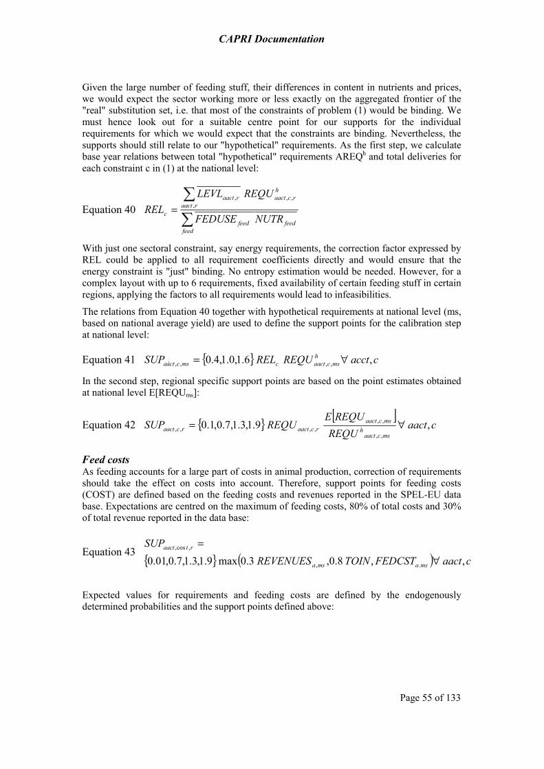
CAPRI Documentation

of 133

Given the large number of feeding stuff, their differences in content in nutrients and prices, we would expect the sector working more or less exactly on the aggregated frontier of the "real" substitution set, i.e. that most of the constraints of problem (1) would be binding. We must hence look out for a suitable centre point for our supports for the individual requirements for which we would expect that the constraints are binding. Nevertheless, the supports should still relate to our "hypothetical" requirements. As the first step, we calculate base year relations between total "hypothetical" requirements AREQh and total deliveries for each constraint c in (1) at the national level:

Equation 40 ∑

∑=

feedfeedfeed

raact

hrcaactraact

c NUTRFEDUSE

REQULEVLREL ,

,,,

With just one sectoral constraint, say energy requirements, the correction factor expressed by REL could be applied to all requirement coefficients directly and would ensure that the energy constraint is "just" binding. No entropy estimation would be needed. However, for a complex layout with up to 6 requirements, fixed availability of certain feeding stuff in certain regions, applying the factors to all requirements would lead to infeasibilities.

The relations from Equation 40 together with hypothetical requirements at national level (ms, based on national average yield) are used to define the support points for the calibration step at national level:

Equation 41 { } cacctREQURELSUP hmscaactcmscaáct ,6.1,0.1,4.0 ,,,, ∀=

In the second step, regional specific support points are based on the point estimates obtained at national level E[REQUms]:

Equation 42 { } [ ]caact

REQUREQUE

REQUSUPmscaact

hmscaact

rcaactrcaact ,9.1,3.1,7.0,1.0,,

,,,,,, ∀=

Feed costs As feeding accounts for a large part of costs in animal production, correction of requirements should take the effect on costs into account. Therefore, support points for feeding costs (COST) are defined based on the feeding costs and revenues reported in the SPEL-EU data base. Expectations are centred on the maximum of feeding costs, 80% of total costs and 30% of total revenue reported in the data base:

Equation 43 { } ( ) caactFEDCSTTOINREVENUESSUP

msamsa

rtaact

,,8.0,3.0max9.1,3.1,7.0,01.0 .,

,cos,

∀=

Expected values for requirements and feeding costs are defined by the endogenously determined probabilities and the support points defined above:

CAPRI Documentation

of 133

Equation 44

cfeedUPPROB

raactUPPROB

rcaactUPPROB

k

k

k

,S]E[NUTR

,S]E[COST

,,S]E[REQU

kc,,feed,kc,feed,cfeed,

kr,cost,aacct,kr,cost,aact,raact,

kr,c,aact,kr,c,aact,rc,aact,

∀⋅=

∀⋅=

∀⋅=

∑

∑

∑

Probabilities observe the adding up conditions:

Equation 45

cfeedPROB

raactPROB

rcaactPROB

k

k

k

,1

,1

,,1

cfeed,

kr,cost,aact,

kr,c,aact,

∀=

∀=

∀=

∑

∑

∑

Following the notation established in part 1, the requirements defined per day and head are covered by:

Equation 46 [ ] [ ] rcaactNUTREFEDNGDAYSREQUEfeed

cfeedrfeedaactraactrcaact ,,,,,,,, ∀≤ ∑

Adding up the fed quantities over the herd sizes, the total feed use per region is defined as

Equation 47 rfLEVLFEDNGFEDUSEaact

raactrfeedaactrfeed ,,,,, ∀== ∑

Since some of the feeding stuffs (silage, gras, other root crops) are assumed to be not tradable between regions, the above equation is treated as an equality constraint where FEDUSE is fixed to the observed production quantities.

For all other feeding stuffs, the following adding up constraints at the national level define binding equality constraints for the calibration process where FEDUSEN defines the exogenously fixed, observed quantities fed at Member State level:

Equation 48 fFEDUSENFEDUSE feedr

feedr ∀=∑ ,

Finally, the objective function with the cross entropy criterion is defined as

Equation 49

∑

∑

∑

−

−

−=

cfeedkcfeedcfeed

kraactkkrtaactkrtaact

krcaactkkrcaactkrcaact

pqPROBPROB

pqPROBPROB

pqPROBPROBPROBH

,,,

,,,,cos,,,cos,

,,,,,,,,,

)log(

)log(

)log()(

The requirements based on the solution of the entropy problem described in part 2 as well as the trade price determination described in part 3 are then integrated in a framework where all the regional supply models for a Member State are linked together. This simultaneous solution is used only once for the calibration step whereas regional models will be solved independently in simulation runs.

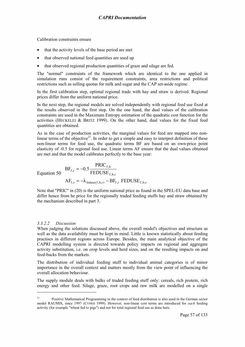
CAPRI Documentation

of 133

Calibration constraints ensure

• that the activity levels of the base period are met

• that observed national feed quantities are used up

• that observed regional production quantities of graze and silage are fed.

The "normal" constraints of the framework which are identical to the one applied in simulation runs consist of the requirement constraints, area restrictions and political restrictions such as selling quotas for milk and sugar and the CAP set-aside regime.

In the first calibration step, optimal regional trade with hay and straw is derived. Regional prices differ from the uniform national price.

In the next step, the regional models are solved independently with regional feed use fixed at the results observed in the first step. On the one hand, the dual values of the calibration constraints are used in the Maximum Entropy estimation of the quadratic cost function for the activities (HECKELEI & BRITZ 1999). On the other hand, dual values for the fixed feed quantities are obtained.

As in the case of production activities, the marginal values for feed are mapped into non-linear terms of the objective21. In order to get a simple and easy to interpret definition of these non-linear terms for feed use, the quadratic terms BF are based on an own-price point elasticity of -0.5 for regional feed use. Linear terms AF ensure that the dual values obtained are met and that the model calibrates perfectly to the base year:

Equation 50

r,b,fr,f)r,b,f(feduser,f

r,b,f

b,fr,f

FEDUSEBFAFFEDUSE

PRIC5.0BF

−λ−=

−=

Note that "PRIC" in (20) is the uniform national price as found in the SPEL-EU data base and differ hence from he price for the regionally traded feeding stuffs hay and straw obtained by the mechanism described in part 3.

3.3.2.2 Discussion When judging the solutions discussed above, the overall model's objectives and structure as well as the data availability must be kept in mind. Little is known statistically about feeding practises in different regions across Europe. Besides, the main analytical objective of the CAPRI modelling system is directed towards policy impacts on regional and aggregate activity substitution, i.e. on crop levels and herd sizes, and on the resulting impacts on and feed-backs from the markets.

The distribution of individual feeding stuff to individual animal categories is of minor importance in the overall context and matters mostly from the view point of influencing the overall allocation behaviour.

The supply module deals with bulks of traded feeding stuff only: cereals, rich protein, rich energy and other feed. Silage, graze, root crops and raw milk are modelled on a single 21 Positive Mathematical Programming in the context of feed distribution is also used in the German sector model RAUMIS, since 1997 (CYPRIS 1999). However, non-linear cost terms are introduced for each feeding activity (for example "wheat fed to pigs") and not for total regional feed use as done here.

CAPRI Documentation

of 133

product basis. Without further remedies, the few linear requirement constraints would result in a quite jumpy behaviour of the regional model. A successful integration with the market module would be impossible. Therefore, prices for regionally traded feed depend on the net trade and PMP-terms are introduced for total regional feed use for each feeding stuff in the supply module.

The quantities fed in the supply module are exogenous fixed variables in the market module which determines the mix of the bulks, for example the share of wheat, barley and maize in the cereals aggregate simultaneously with the prices for the components (BRITZ 1998). The elasticities used in double log functions determining the shares are partly based on estimated cost functions for the German feed compound industry (BRITZ & SIEBER 1998). The resulting new price for the bulks as well as their new nutrient content are then handed back in the next overall model iteration to the supply module.

The overall structure is hence a mixture of primal and dual approaches. Hopefully, the solution mainly integrates the advantages of the different solutions instead of combining all possible draw-backs.

3.4 Input allocation for fertilisers and nutrient balances

In the following section, the existing environmental indicators in CAPRI, planned and already achieved improvements, and possible further extensions are briefly discussed. It should be noted that CAPRI is basically a regionalised agricultural sector model, thus concentrating on the modelling of aggregated reactions of agricultural producers and consumers to changes in long term shifters as technical progress, income changes and CAP programs. Most indicators are rather robust pressure indicators and can be calculated easily based on fixed parameters approaches from the endogenous variables of the regional aggregate supply models. Accordingly, economic (dis)-incentives can be linked to the pressure indicators or further passive indicators can be introduced or the current ones changed easily.

So far, the link between instruments of agri-environmental instruments and pressure indicators had been explored for the case of greenhouse gas emissions (Pérez 2005). During the first phase of CAPRI (1996-1999), NPK balances and output of greenhouse gases had been introduced, and an energy use indicator was explored for Switzerland. The project for DG-ENV (2001-2002) then led to (1) the improvement of the current state indicators -especially ammonia output and nitrate leaching, (2) the introduction of new ones as a water balances and chemical indicators, (3) feasibility studies for the application of the Nutrient Flow Model for the Netherlands and the bio-physical model CropSyst for regions in France, and (4) improving the interpretation of environmental indicators by contrasting them with soil and land-use maps. The following table shows an overview of the indicators embedded in the CAPRI system after the finalisation of the DG-ENV project.

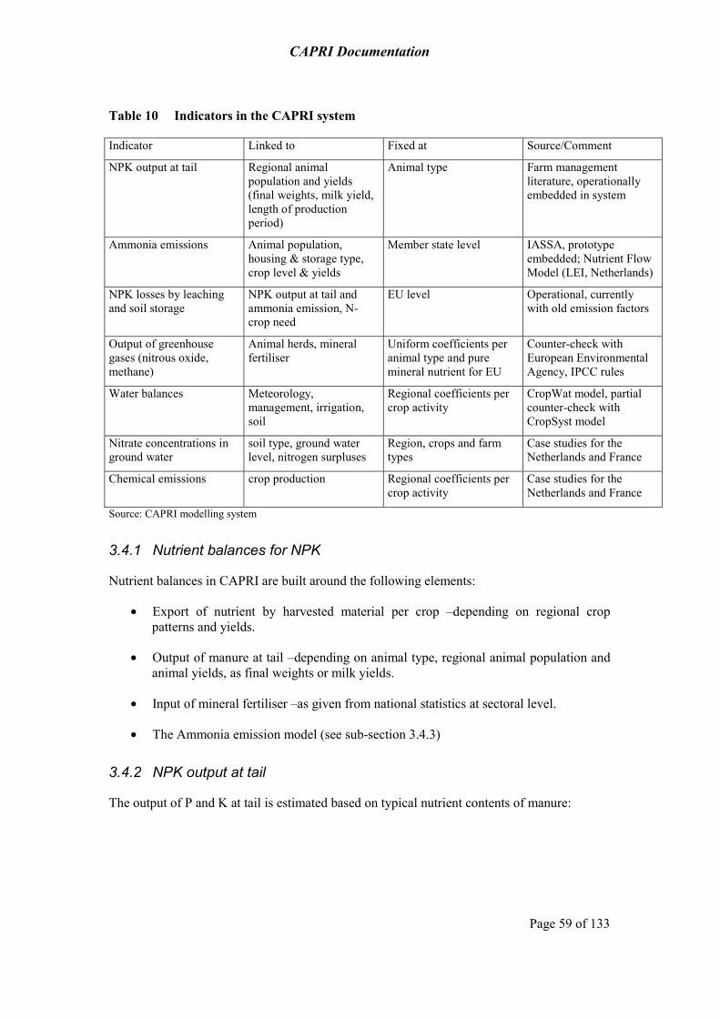
CAPRI Documentation

of 133

Table 10 Indicators in the CAPRI system

Indicator Linked to Fixed at Source/Comment

NPK output at tail Regional animal population and yields (final weights, milk yield, length of production period)

Animal type Farm management literature, operationally embedded in system

Ammonia emissions Animal population, housing & storage type, crop level & yields

Member state level IASSA, prototype embedded; Nutrient Flow Model (LEI, Netherlands)

NPK losses by leaching and soil storage

NPK output at tail and ammonia emission, N-crop need

EU level Operational, currently with old emission factors

Output of greenhouse gases (nitrous oxide, methane)

Animal herds, mineral fertiliser

Uniform coefficients per animal type and pure mineral nutrient for EU

Counter-check with European Environmental Agency, IPCC rules

Water balances Meteorology, management, irrigation, soil

Regional coefficients per crop activity

CropWat model, partial counter-check with CropSyst model

Nitrate concentrations in ground water

soil type, ground water level, nitrogen surpluses

Region, crops and farm types

Case studies for the Netherlands and France

Chemical emissions crop production Regional coefficients per crop activity

Case studies for the Netherlands and France

Source: CAPRI modelling system

3.4.1 Nutrient balances for NPK

Nutrient balances in CAPRI are built around the following elements:

• Export of nutrient by harvested material per crop –depending on regional crop patterns and yields.

• Output of manure at tail –depending on animal type, regional animal population and animal yields, as final weights or milk yields.

• Input of mineral fertiliser –as given from national statistics at sectoral level.

• The Ammonia emission model (see sub-section 3.4.3)

3.4.2 NPK output at tail

The output of P and K at tail is estimated based on typical nutrient contents of manure:

CAPRI Documentation

of 133

Table 11 Nutrient content in manure in kg pure nutrient/m³

P K

Cattle 2.0 5.5

Swine 3.3 3.3

Poultry 6.3 5.1 Source: Lufa von Weser-Ems, Stand April 1990, Naehrstoffanfall.

These data are converted into typical pure nutrient emission at tail per day and kg live weight in order to apply them for the different type of animals. For cattle, it is assumed that one live stock unit (=500 kg) produces 18 m³ manure per year, so that the numbers in the table above are multiplied with 18 m³ and divided by (500 kg *365 days).

For the different types of cattle activities, it is hence necessary to determine the average live weight and the length of the production process.

For calves fattening (CAMF, CAFF), the carcass weight is divided by 60 % in order to arrive at final weight and a start weight of 50 kg is assumed. Daily weight increases are between 0.8 kg/day and 1.2 kg/day and depend proportionally on average stocking densities of cattle in relation to the average EU stocking density for which a daily weight increase of 1 kg/day is assumed. Total emissions per animal hence increase with final weights but decrease per kg of meat produced for intensive production systems with high daily weight increases. The same relationship holds for all other animal categories discussed in the following paragraphs.

For calves raising (CAMR, CAFR), two periods are distinguished. From 50 to 150 kg, a daily increase of 0.8 kg/day is assumed. The remaining period captures the growth from 151 to 335 kg for male and 330 kg for female calves, where the daily increase is between 1 kg/day and 1.4 kg/day, again depending on stocking densities.

The bull fattening process captures the period from 335 kg live weight to final weight. Daily increases are between 0.8 kg/day up to 1.4 kg/day, depending on final weights and stocking densities. Carcass weights as reported in the data base are re-converted into live weight assuming a factor of 54% for low and 57% for higher final weights.

The heifers fattening process captures the period from 300 kg live weight to final weight, assuming a daily increase of 0.8 kg/day. Carcass weights, as reported in the data base, are re-converted into live weight assuming a factor of 54 % for low and 57 % for higher final weights.

Suckler cows are assumed to be whole year long in production and weight 550 kg, whereas milk cows are assumed to have a weight of 600 kg and are again for 365 days in production. Additional data relate to the additional NPK output per kg milk produced by cows and are taken from the RAUMIS model:

Table 12 Additional emission of NPK per kg of milk produced

N 0.0084

P 0.004

K 0.0047 Source: RAUMIS Model (http://www.agp.uni-bonn.de/agpo/rsrch/raumis_e.htm).

CAPRI Documentation

of 133

The factors shown above for pigs are converted into a per day and live weight factor for sows by assuming a production of 5 m³ of manure per sow (200 kg sow) and 15 piglets at 10 kg over a period of 42 days. Consequently, the manure output of sows varies in the model with the number of piglets produced.

For pig fattening processes, it is assumed that 1.9 m³ are produced per ‘standard’ pig with a final carcass weight of 90 kg at 78 % meat content, a starting weight of the fattening period of 20 kg (weight of the piglet), a production period of 143 days and 2.3 rounds per year. The actual factors used depend on tables relating the final weight to typical daily weight increases.

For poultry, it is assumed that 8 m³ of manure are produced by 100 laying hens, which are assumed to weigh 1.9 kg and stay for 365 days in production. For poultry fattening processes, a fattening period of 49 days to reach 1.9 kg is assumed.

For sheep and goat used for milk production or as mother animals, the cattle factors are applied by assuming a live weight of 57.5 kg and 365 days in production. For fattening processes, a daily increase of 200 kg and a meat content of 60 % of the carcass weight are assumed.

The nitrogen emission factors from animal activities are coupled to crude protein intake (IPCC 1997). According to the literature (Udersander et al. 1993), there is a relation of 1 to 6 between crude protein and N in feeding . By combining this information with N retention rates per animal activity (IPCC 2000, table 4.15), manure production rates can be estimated (N intake minus N retention).

Table 13 Crude protein intake, manure production and nitrogen retention per head

(EU 15, year 2001)

Crude protein

Nitrogen in manure

Nitrogen retention

BULH 1.7 83.8 0.07 BULL 1.4 31.7 0.07 CAFF 0.8 21.5 0.07 CAFR 0.9 38.4 0.07 CAMF 0.8 20.2 0.07 CAMR 0.9 38.6 0.07 DCOH 4.3 210.1 0.20 DCOL 2.7 129.4 0.20 HEIH 1.5 64.4 0.07 HEIL 1.2 20.6 0.07 HEIR 1.7 95.9 0.07 HENS (1000 units) 21.2 900.9 0.30 PIGF 0.4 7.0 0.30 POUF (1000 units) 7.6 52.9 0.30 SHGM 0.2 13.7 0.10 SHGF 0.1 2.0 0.10 SOWS 0.9 36.4 0.30 SCOW 1.5 87.2 0.07


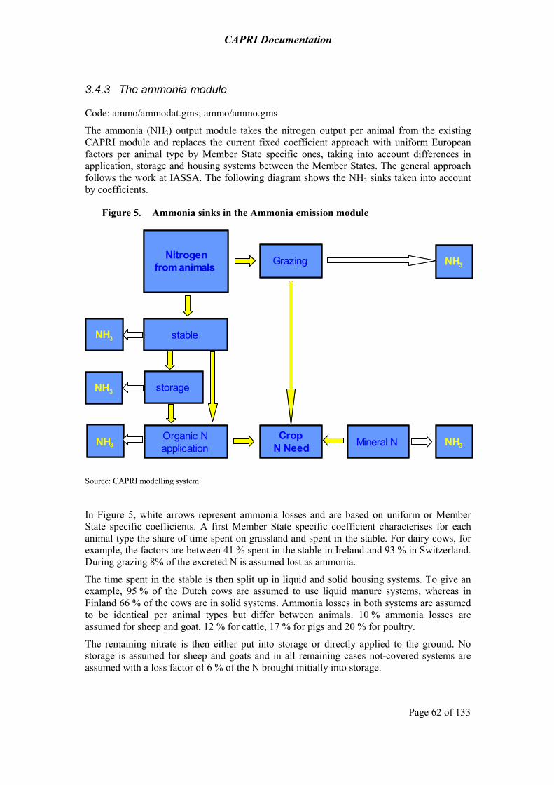
CAPRI Documentation

of 133

3.4.3 The ammonia module

Code: ammo/ammodat.gms; ammo/ammo.gms

The ammonia (NH3) output module takes the nitrogen output per animal from the existing CAPRI module and replaces the current fixed coefficient approach with uniform European factors per animal type by Member State specific ones, taking into account differences in application, storage and housing systems between the Member States. The general approach follows the work at IASSA. The following diagram shows the NH3 sinks taken into account by coefficients.

Figure 5. Ammonia sinks in the Ammonia emission module

Nitrogen from animals

Crop N Need

Nitrogen from animals

Crop N Need NH 3 Mineral N NH 3 Mineral N

Grazing

stable NH 3

NH 3 Grazing

stable NH 3

NH 3

storage NH 3 storage NH 3

Organic N application NH 3 Organic N application NH 3


In Figure 5, white arrows represent ammonia losses and are based on uniform or Member State specific coefficients. A first Member State specific coefficient characterises for each animal type the share of time spent on grassland and spent in the stable. For dairy cows, for example, the factors are between 41 % spent in the stable in Ireland and 93 % in Switzerland. During grazing 8% of the excreted N is assumed lost as ammonia.

The time spent in the stable is then split up in liquid and solid housing systems. To give an example, 95 % of the Dutch cows are assumed to use liquid manure systems, whereas in Finland 66 % of the cows are in solid systems. Ammonia losses in both systems are assumed to be identical per animal types but differ between animals. 10 % ammonia losses are assumed for sheep and goat, 12 % for cattle, 17 % for pigs and 20 % for poultry.

The remaining nitrate is then either put into storage or directly applied to the ground. No storage is assumed for sheep and goats and in all remaining cases not-covered systems are assumed with a loss factor of 6 % of the N brought initially into storage.

CAPRI Documentation

of 133

After storage, the remaining N is applied to the soil, either spread to the surface –losses at 20% or using application techniques with lower (15%) or high (10%) emission reductions. Currently, it is assumed that all farmers work with the standard techniques.

Technically, the underlying calculations are embedded as GAMS code in an own module both called during updates of the data base and model runs. The relevant coefficients are stored as a separate table, a transparent solution allowing to quickly perform sensitivity analysis or updating them.

Table 14 Nitrogen balance (EU 15, year 2001)

INPUT OUTPUT

Import of nitrogen by anorganic fertiliser a 68.2 Export of nitrogen with

harvested material f 80.95

Import of nitrogen by organic fertiliser (in manure)

b 77.31 Nitrogen in ammonia losses from manure fallen on grazings g 2.08

Nitrogen from biological fixation* c 2.89 Nitrogen in ammonia losses

from manure in stable h 7.13

Nitrogen from atmospheric deposition d 14.36 Nitrogen in ammonia losses

from manure storage i 2.53

Nitrogen in ammonia losses

from manure application on the field

j 8.34

Nitrogen in ammonia losses from organic fertiliser k=g+h+i+j 20.08

Nitrogen in ammonia losses from mineral fertiliser l 2.89

TOTAL INPUT e=a+b+c+d 162.768 TOTAL OUTPUT n=f+k+l+m 103.92

Nutrient losses at soil level (SURPLUS) m=e-f-k-l 58.85


3.4.4 Input allocation of organic and inorganic NPK and the nutrient balance

The input allocation of organic and inorganic fertilizer determines how much NPK organic and inorganic fertiliser is applied per ha of a crop, simultaneously estimating the NPK availability in manure. Firstly, nutrient export by the harvested material is determined, based on the following factors:

Table 15 Exports of nutrients in kg per ton of yield or constant Euro revenues

N P K

Soft wheat 20 8 6

Durum wheat 23 8 7

Rye 15 8 6

Barley 15 8 6

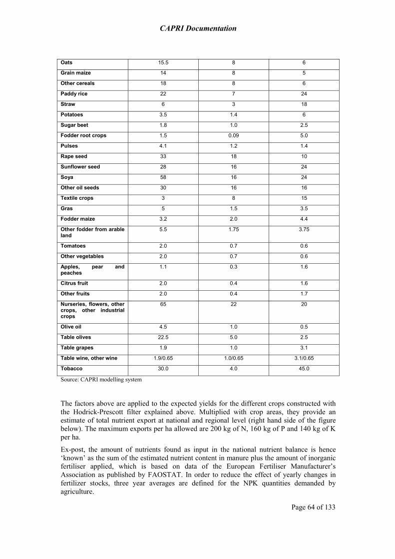
CAPRI Documentation

of 133

Oats 15.5 8 6

Grain maize 14 8 5

Other cereals 18 8 6

Paddy rice 22 7 24

Straw 6 3 18

Potatoes 3.5 1.4 6

Sugar beet 1.8 1.0 2.5

Fodder root crops 1.5 0.09 5.0

Pulses 4.1 1.2 1.4

Rape seed 33 18 10

Sunflower seed 28 16 24

Soya 58 16 24

Other oil seeds 30 16 16

Textile crops 3 8 15

Gras 5 1.5 3.5

Fodder maize 3.2 2.0 4.4

Other fodder from arable land

5.5 1.75 3.75

Tomatoes 2.0 0.7 0.6

Other vegetables 2.0 0.7 0.6

Apples, pear and peaches

1.1 0.3 1.6

Citrus fruit 2.0 0.4 1.6

Other fruits 2.0 0.4 1.7

Nurseries, flowers, other crops, other industrial crops

65 22 20

Olive oil 4.5 1.0 0.5

Table olives 22.5 5.0 2.5

Table grapes 1.9 1.0 3.1

Table wine, other wine 1.9/0.65 1.0/0.65 3.1/0.65

Tobacco 30.0 4.0 45.0


The factors above are applied to the expected yields for the different crops constructed with the Hodrick-Prescott filter explained above. Multiplied with crop areas, they provide an estimate of total nutrient export at national and regional level (right hand side of the figure below). The maximum exports per ha allowed are 200 kg of N, 160 kg of P and 140 kg of K per ha.

Ex-post, the amount of nutrients found as input in the national nutrient balance is hence ‘known’ as the sum of the estimated nutrient content in manure plus the amount of inorganic fertiliser applied, which is based on data of the European Fertiliser Manufacturer’s Association as published by FAOSTAT. In order to reduce the effect of yearly changes in fertilizer stocks, three year averages are defined for the NPK quantities demanded by agriculture.

CAPRI Documentation

of 133

For Nitrogen, ammonia losses are explicitly handled as taken from the Nutrient Flow Model developed by LEI and contributed by the project financed by DG-ENV. Remaining losses could either be run-off (leaching or accumulation in soil) and as non-ammonia gas losses (nitrous oxide). Additional sources of N are taken into account as well.

Table 16 Atmospheric deposition of N per kg and year

Austria 20

Belgium 32

Denmark 18

Finland 5

France 16

Germany 29

United Kingdom 15

Greece 7

Irland 10

Italy 12

Netherlands 36

Norway 5

Portugal 3

Spain 6

Sweden 5

Switzerland 18


Figure 6 offers a graphical representation of these relationships.

CAPRI Documentation

of 133

Figure 6. Ex-post calibration of NPK balances and the ammonia module

Posterioridensity estimator

% Organic availabilityNet of NH3 losses

% fertilisationOver export

Posterioridensity estimator

% Organic availabilityNet of NH3 losses

% fertilisationOver export

Outputat tail

Manure outputfunctions

Herd sizesFinal weights etc.

NH3-LossesOrganic

Outputat tail

Manure outputfunctions

Herd sizesFinal weights etc.

NH3-LossesOrganic

Atmosphericdeposition

Nutrientexport

Nutrient contentof harvest

Crop areasyields

Nutrientexport

Nutrient contentof harvest

Crop areasyields

Biologicalfixation

Biologicalfixation

Use= Use=

National mineralfertiliser use

NH3-LossesAnorganic

National mineralfertiliser use

NH3-LossesAnorganic

DeliveriesDeliveries


The following equations comprise together the cross-entropy estimator for the NPK (Fnut=N, P or K) balancing problem. Firstly, the purchases (NETTRD) of anorganic fertiliser for the regions must add up to the given inorganic fertiliser purchases at Member State level:

Equation 51 ∑=r

Fnutr

FnutMS NettrdNettrd

The crop need –minus biological fixation for pulses– multiplied with a factor describing fertilisation beyond exports must be covered by:

(1) inorganic fertiliser, corrected by ammonia losses during application in case of N,

(2) atmospheric deposition, taking into account a crop specific loss factor in form of ammonia, and

(3) nutrient content in manure, corrected by ammonia losses in case of N, and a specific availability factor.

Equation 52

( )( )

( )∑

∑

−−+

+

−=

∈∧+

−

aactfnutr

ManurerFnutaactraactr

AtmDepCact

AtmDepr

AnogrFnut

Fnutr

cact fnutrfnutr

biofixcactFnutcactrcactr

NavFacLossNHFnutLevl

NFactNBal

LossNHNETTRD

graigraeofarcactNutFacGNutFac

NFactFnutLevl

,,,,

,

,,

,,,

1)31(

)31(

,,1

1

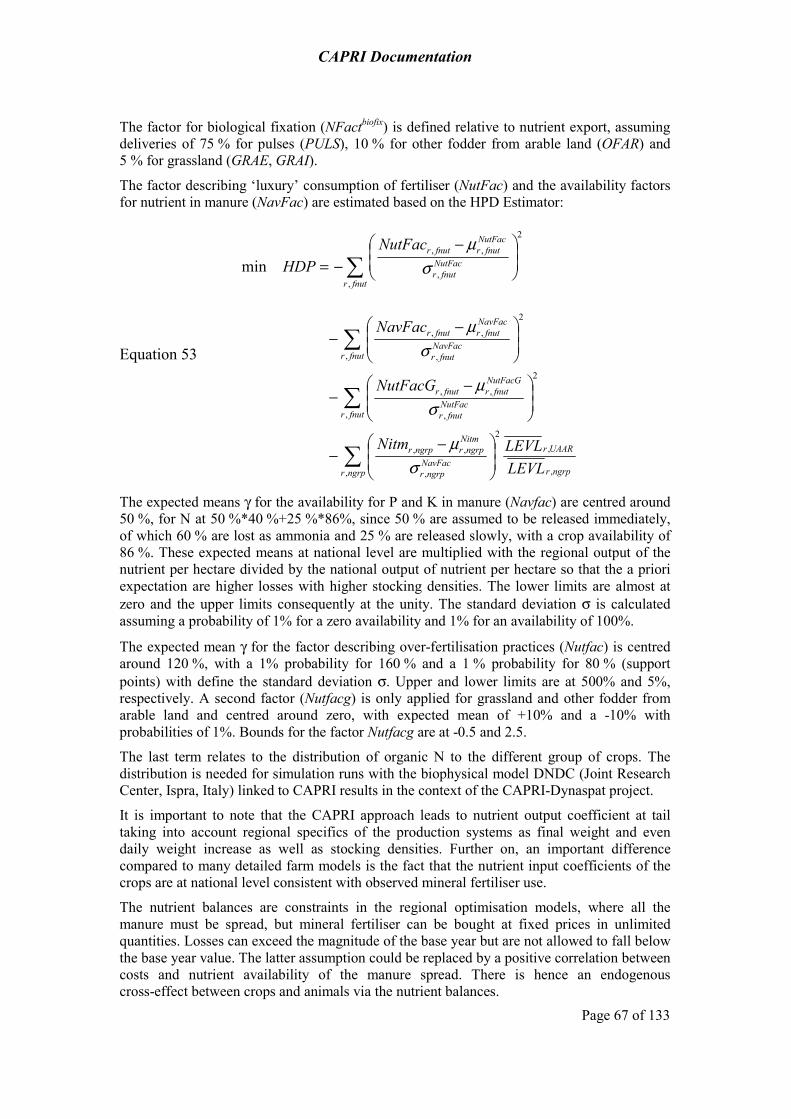
CAPRI Documentation

of 133

The factor for biological fixation (NFactbiofix) is defined relative to nutrient export, assuming deliveries of 75 % for pulses (PULS), 10 % for other fodder from arable land (OFAR) and 5 % for grassland (GRAE, GRAI).

The factor describing ‘luxury’ consumption of fertiliser (NutFac) and the availability factors for nutrient in manure (NavFac) are estimated based on the HPD Estimator:

Equation 53

∑

∑

∑

∑

⎟⎟⎠

⎞⎜⎜⎝

⎛ −−

⎟⎟⎠

⎞⎜⎜⎝

⎛ −−

⎟⎟⎠

⎞⎜⎜⎝

⎛ −−

⎟⎟⎠

⎞⎜⎜⎝

⎛ −−=

ngrpr ngrpr

UAARrNavFac

ngrpr

Nitmngrprngrpr

fnutrNutFac

fnutr

NutFacGfnutrfnutr

fnutrNavFac

fnutr

NavFacfnutrfnutr

fnutr

NutFacfnutr

NutFacfnutrfnutr

LEVLLEVLNitm

NutFacG

NavFac

NutFacHDP

, ,

,2

,

,,

,

2

,

,,

,

2

,

,,

,

2

,

,,

min

σµ

σµ

σµ

σµ

The expected means γ for the availability for P and K in manure (Navfac) are centred around 50 %, for N at 50 %*40 %+25 %*86%, since 50 % are assumed to be released immediately, of which 60 % are lost as ammonia and 25 % are released slowly, with a crop availability of 86 %. These expected means at national level are multiplied with the regional output of the nutrient per hectare divided by the national output of nutrient per hectare so that the a priori expectation are higher losses with higher stocking densities. The lower limits are almost at zero and the upper limits consequently at the unity. The standard deviation σ is calculated assuming a probability of 1% for a zero availability and 1% for an availability of 100%.

The expected mean γ for the factor describing over-fertilisation practices (Nutfac) is centred around 120 %, with a 1% probability for 160 % and a 1 % probability for 80 % (support points) with define the standard deviation σ. Upper and lower limits are at 500% and 5%, respectively. A second factor (Nutfacg) is only applied for grassland and other fodder from arable land and centred around zero, with expected mean of +10% and a -10% with probabilities of 1%. Bounds for the factor Nutfacg are at -0.5 and 2.5.

The last term relates to the distribution of organic N to the different group of crops. The distribution is needed for simulation runs with the biophysical model DNDC (Joint Research Center, Ispra, Italy) linked to CAPRI results in the context of the CAPRI-Dynaspat project.

It is important to note that the CAPRI approach leads to nutrient output coefficient at tail taking into account regional specifics of the production systems as final weight and even daily weight increase as well as stocking densities. Further on, an important difference compared to many detailed farm models is the fact that the nutrient input coefficients of the crops are at national level consistent with observed mineral fertiliser use.

The nutrient balances are constraints in the regional optimisation models, where all the manure must be spread, but mineral fertiliser can be bought at fixed prices in unlimited quantities. Losses can exceed the magnitude of the base year but are not allowed to fall below the base year value. The latter assumption could be replaced by a positive correlation between costs and nutrient availability of the manure spread. There is hence an endogenous cross-effect between crops and animals via the nutrient balances.

CAPRI Documentation

of 133

The factors above together with the regional distribution of the national given inorganic fertiliser use are estimated over a time series. Trend lines are regressed though the resulting time series of manure availability factors of NPK and crop nutrient factors for NPK, and the resulting yearly rates of change are used in simulation to capture technical progress in fertiliser application. The following table shows a summary by highlighting which elements of the NPK are endogenous and exogenous during the allocation mechanism and during model simulations:

Table 17 Table: Elements entering the of NPK balance ex-post and ex-ante

Ex-post Ex_ante

• Given:

– Herd sizes => Manure output

– Crop areas and yields => Export with harvest

– National anorganic application

• Estimated:

– Regional anorganic application

– Factor for Fertilization beyond N export

– Manure availability

• Model result:

– Herd sizes => manure output

– Crop areas and yields => Export with harvest

– National and Regional anorganic application

• Given:

– Factor for Fertilization beyond export (trended)

– Manure availability (trended)


3.4.5 Greenhouse Gases

For the purpose of modelling GHG emissions from agriculture, a multi-strategy approach is followed. It is important to take into account that agriculture is an important emitter of several climate relevant gases other than carbon dioxide. Therefore, two types of pollutants are modelled: methane (CH4) and nitrous oxide (N2O). The sources considered are: CH4 emissions from animal production, manure management and rice cultivation and N2O from agricultural soils and manure management22.

In CAPRI consistent GHG emission inventories for the European agricultural sector are constructed. As already mentioned, land use and nitrogen flows are estimated at a regional level. This is the main information needed to calculate the parameters included in the IPCC Good Practice Guidance (IPCC, 2000). The following table lists the emission sources modelled:

22 Carbon sinks are not included since the measurement of carbon dioxide absorption through agricultural biomass is highly complex (high uncertainty involved, especially in agricultural soils) and has strong linkages with other economic activities not considered in this analysis, such as bio-diesel production and forestry management.

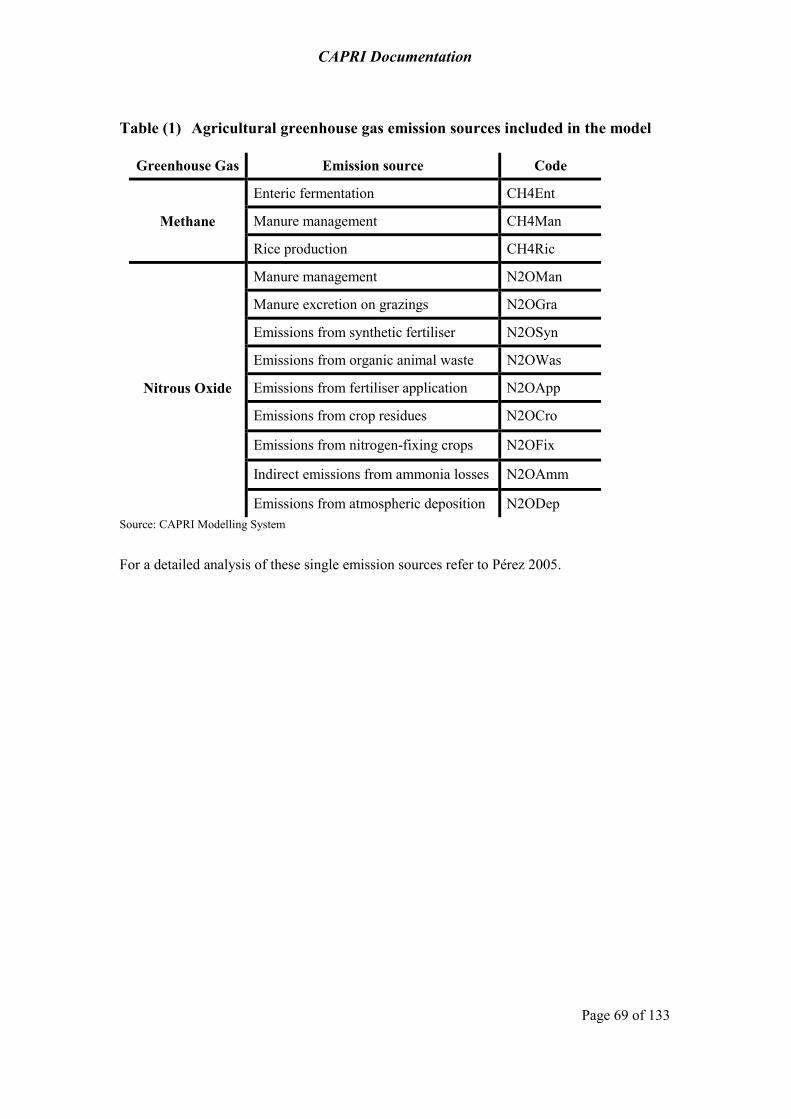
CAPRI Documentation

of 133

Table (1) Agricultural greenhouse gas emission sources included in the model

Greenhouse Gas Emission source Code

Enteric fermentation CH4Ent

Methane Manure management CH4Man

Rice production CH4Ric

Manure management N2OMan

Manure excretion on grazings N2OGra

Emissions from synthetic fertiliser N2OSyn

Emissions from organic animal waste N2OWas

Nitrous Oxide Emissions from fertiliser application N2OApp

Emissions from crop residues N2OCro

Emissions from nitrogen-fixing crops N2OFix

Indirect emissions from ammonia losses N2OAmm

Emissions from atmospheric deposition N2ODep Source: CAPRI Modelling System

For a detailed analysis of these single emission sources refer to Pérez 2005.

CAPRI Documentation

of 133

4 Baseline Generation Model (CAPTRD)

Code: captrd.gms

The aim of the CAPRI projection tool is to provide a baseline used as comparison points or comparison time series for counterfactual analysis. The baseline may be interpreted as a projection in time covering the most probable future development or the European agricultural sector under the status-quo policy and including all future changes already foreseen in the current legislation.

Conceptually, the baseline should capture the complex interrelations between technological, structural and preference changes for agricultural products world-wide in combination with changes in policies, population and non-agricultural markets. Given the complexity of these highly interrelated developments, baselines are in most cases not a straight outcome from a model but developed in conjunction of trend analysis, model runs and expert consultations. In this process, model parameters such as e.g. elasticities and exogenous assumptions such as e.g. technological progress captured in yield growth are adjusted in order to achieve plausible results (as regarded by experts, e.g. European Commission projections). It is almost unavoidable that the process is somewhat intransparent. Two typical examples are discussed here.

− In the case of the AgLink modelling system of the OECD, questionnaires are sent out to the OECD Member States covering all endogenous and exogenous variables of AgLink. The Member States fill in time series regarding the future developments for their respective countries. The values inputted may stem themselves from country specific model baselines, expert consultations, trend analyses or other sources –in many cases, their provenience is not known in detail. The OECD then sets the constant terms in all behavioural equations of AgLink so that the country modules would exactly recover the values for the endogenous variables for that country found in the questionnaires at the values inputted for the exogenous variables. Clearly, as the countries will fill in their questionnaire without knowing about the future expectations of other OECD Members, the expectations of the different teams e.g. regarding imports/exports or world market prices may differ and lead to values at country level which are mutually not compatible when linked globally together in the modelling framework. To eliminate such differences, the OECD will repeatedly start AgLink to generate technically compatible results and receive comments on these runs which will lead to updated data in the questionnaires and thus new shift terms in the behavioural equations.

− The second example is that of FAPRI where a so-called melting down meeting is organised where the modellers responsible for specific parts of the system come together with market experts. Results are discussed, parameters and assumptions changed until there is consensus. Little is known about how the process works exactly, but both examples underline the interaction between model mechanism and ex-ante expectations of market experts.

This section explains in detail the methodology used in CAPRI to construct a baseline. Before entering into these details it should be stated that ultimately almost any projection may be reduced to a particular type of trend projections, at least if the exogenous inputs, such as population, prices or household expenditure are also projected (usually by other research teams) as functions of time. In this sense trend projection may provide a firm ground on which to build projections and this is exactly their purpose in our work. These trends are supplemented in the CAPRI baseline tools with results from other baselines, especially from DG-AGRI.

CAPRI Documentation

of 133

The projection tool is fed both by forecasts from different experts or modelling tools, as well by trend forecasts using data from the ‘COCO’ database23 as ex-post information. The purpose of these trend estimates is, on the one hand, to compare expert forecasts with a purely technical prolongation of time series and, on the other hand, to provide a ‘safety net’ position in case no values from external projection are available. Therefore, trend variables for baseline generation in the model are mainly constructed out of expert data on projections (e.g. FAO, European Commission or World Bank) and linear trends of data contained in the CAPRI data base. These trend variables are simultaneously subject to the consistency restrictions imposed by the mathematical programming model and not made as independent forecasts for each time series (e.g. closed area and market balances). The resulting estimator is hence a system estimator under constraints whose properties are discussed in the following section. Nonetheless it is to be acknowledged here that the trend remain mechanical in that they try to respect technological relationships but remain ignorant about behavioural functions or policy developments24.

4.1 Trend curve

The first ingredient in the estimator is the trend curve itself which is defined as:

Equation 54 jircjirjir

Trendjtir tbaX ,,

,,,,,,, +=

where the parameters a, b and c are to be estimated so that the squared deviation between given and estimated data are minimized. The X stands for the data and represents a five dimensional array, spanning up products i and items j (as feed use or production), regions r, points in time t and different data status as ‘Trend’ or ‘Observed’. The trend curve itself is a kind of Box-Cox transformation, as parameter c is used as the exponent of the trend. For c equal unity, the resulting curve is a straight line, for c between 0 and 1, the curve is concave from below, i.e. increasing but with decreasing rates, whereas for c > 1, the curve is convex from below, i.e. increasing with increasing rates. In order to prevent differences between time points to increase sharply over the projection period, the parameters c are restricted to be below 1.2.

In a first prototype of the module, a polynomial trend curve of degree two was evaluated. However, a quadratic function is not necessarily monotone on the forecast interval so that a trend curve may for example show increasing yields for the first part of the projection period and afterwards a decrease. As such outcomes are purely technical and not motivated by a priori knowledge, it was deemed more plausible to switch to the formulation shown above with the same number of free parameters as a quadratic trend curve, but with monotony guaranteed.

The ex-post period covers the period from 1985 towards 2000. In order to cut down the size of the resulting problem, the ex-ante period is defined in ten years steps (2003, 2010, 2020, 2030), as intermediate years can be simply calculated once the estimated parameters are known.

23 Britz, W., Wieck, C., Jansson, T. (2002): National framework of the CAPRI-data base - the COCO – Module, CAPRI Working Paper 02-04, Institute of Agricultural Policy, Bonn. 24 The only exception is the quota regime on the milk market which has been recognised in the trend projections in that the milk production has been derived from the quota endowments (where current quotas are assumed to persist until 2025).

CAPRI Documentation

of 133

4.2 Consistency constraints in the trend projection tool

The constraints in the trend projection enforce mutual compatibility between baseline forecasts for individual series in the light of relations between these series, either based on definitions as ‘production equals yield times area’ or on technical relations between series as the balance between energy deliveries from feed use and energy requirements from the animal herds. The set of constraints is deemed to be exhaustive in the sense as any further restriction would either not add information or require data beyond those available. The underlying data set takes into account all agricultural activities and products according to the definition of the Economic Accounts for Agriculture.

The constraints discussed in the following can be seen as a minimum set of consistency conditions necessary for a projection of agricultural variables. As discussed above in detail, the full projection tool features further constraints especially relating to price feedbacks on supply and demand.

4.2.1 Constraints relating to market balances and yields

Closed market balances define the first set of constraints and state that the sum of imports (IMPT) and production (GROF) must be equal to the sum of feed (FEDM) and seed (SEDM) use, human consumption (HCOM), processing (INDM,PRCM), losses (LOSM) and exports (EXPT):

Equation 55

,IMPT,Trend GROF,Trendr,i,t r,i,t

FEDM,Trend SEDM,Trend PRCM,Trend INDM,Trendr,i,t r,i,t r,i,t r,i,tLOSM,Trend HCOM,Trend ,EXPT,Trendr,i,t r,i,t r,i,t

X X

X X X X

X X X

+ =

+ + +

+ +

Where r are the Member States of the EU, i are the products, t the different forecasting years. All elements of the market balances are expressed as primary product equivalents according to the concept of ‘supply utilization accounts’. Human consumption of wheat does hence include floor, bread, pasta etc. recalculated into what equivalent based on conversion factors. The only expectations are oilseeds, where processing to cakes and oils is explicitly covered, and raw milk, where again, processing to the different dairy products is included explicitly.

Secondly, production (GROF) is equal to yield times area/herd size (LEVL) where acts are all production activities:

Equation 56 ∑=acts

TrendactstLEVLr

Trendactstir

TrendGROFtir XXX ,

,,,

,,,

,,

A set of equations relates to the hectares for groups of crop activities (cereals, oilseeds, industrial crops, vegetables, fresh fruits, total vineyards, fodder production on arable land). It defines e.g. that the total hectares of cereals is equal to the sum of hectares for the individual cereals as soft wheat, durum wheat, barley and so forth.

Equation 57 ∑∈

=grpcropj

TrendjtLEVLr

TrendgrpcroptLEVLr XX

_

,,,

,_,,

Equally, the market balance positions for certain products enter adding up equations for groups of products (cereals, oilseeds, industrial crops, vegetables, fresh fruits, total vineyards, fodder production, meat). As an example, total cereal production is equal to the sum over the produced quantities of the individual cereals.

CAPRI Documentation

of 133

Equation 58 ∑∈

=grpproi

TrendMrkBaltir

TrendMrkBaltgrppror XX

_

,,,

,,_,

4.2.2 Constraints relating to agricultural production

Adding up over the individual crop areas defines the total utilizable agricultural area (UAAR,LEVL):

Equation 59 ∑=crops

TrendcropstLEVLr

TrendUAARtLEVLr XX ,

,,,

,,

Further constraints link the different animal activities over young animal markets:

Equation 60 ∑↔

=oyaniiyani

TrendGROFtiyanir

TrendGROFtoyanir XX ,

,,,,,

Where oyani stands for the different young animals defined as outputs (young cows, young bulls, young heifers, male/female calves, piglets, lambs and chicken). These outputs are produced by raising processes, and used as inputs in the other animal processes (fattening, raising or milk producing).

Finally, balances for energy and protein requirements for each animal type maact are introduced as:

Equation 61 ( )Trendmaacttyieldr

Contmaact

Contmaact

tTrendConttfeedr

feed

Trendmaacttfeedr XaaXX ,

,,,

,,,,, 996.0 +=∑

where Cont are the contents in terms of energy and crude protein. The left hand side of the equation defines total delivery of energy or protein from the current feeding practise per animal activity in region r, whereas the right hand side the need per animal derived from requirement functions depending on the main output (meat, milk, eggs, piglets born). The parameters a and b of the requirement functions are estimated from engineering functions as implemented in the CAPRI modelling system, and scaled so that the balance holds for the basis period. The factor in front of the requirements introduces some input saving technical progress of -0.4% per annum.

The feeding coefficients multiplied with the herd sizes define total feed use for the different feeding stuffs ‘bulks’ (cereals, protein rich, energy rich, dairy based, other) and single non-tradable feed (grass, maize silage, fodder root crops, straw, milk for feeding, other fodder from arable land):

Equation 62 Trendmaacttlevlr

maact

Trendmaacttfeedr

TrendFEDMtfeedr XXX ,

,"",,,,

,,, ∑=

Finally, the feed use of individual products must add up to the feed use of the ‘bulks’ mentioned above:

Equation 63 ∑→

=fedo

TrendFEDMttor

TrendFEDMtfeedr XX ,

,,,

,,

4.2.3 Constraints relating to prices, production values and revenues

The check of external forecasts revealed that for some products, price projections are not available. It was decided to include prices, value and revenues per activity in the constrained

CAPRI Documentation

of 133

estimation process. The first equation defines the value (EAAG, position from the Economic Accounts for Agriculture) of each product and product group as the product of production (GROF) times the unit value prices (UVAG):

Equation 64 TrendUVAGtir

TrendGROFtir

TrendEAAGtir XXX ,

,,,

,,,

,, =

The revenues of the activities (TOOU, total output) for each activity and group of activities acts are defined as:

Equation 65 ∑=o

TrendUVAGtor

Trendactstor

TrendactstTOOUr XXX ,

,,,

,,,

,,

As for the market balances, the values for certain aggregate product groups must add up:

Equation 66 ∑∈

=grpproi

TrendEAAGtir

TrendEAAGtgrppror XX

_

,,,

,,_,

Consumer prices (UVAD) are equal to producer prices (UVAG) plus a margin (CMRG):

Equation 67 TrendCMRGtir

TrendUVAGtir

TrendUVADtir XXX ,

,,,

,,,

,, +=

4.2.4 Constraints relating to consumer behaviour

Human consumption (HCOM) is defined as per head consumption multiplied with population:

Equation 68 TrendINHAtLEVLr

TrendINHAtir

TrendHCOMtir XXX ,

,,,

,,,

,, =

Consumer expenditures per caput (EXPE) are equal to human consumption per caput (INHA) times consumer prices (UVAD):

Equation 69 TrendUVADtLEVLr

TrendINHAtir

TrendEXPEtir XXX ,

,,,

,,,

,, =

As for the market balances, the per caput expenditure (EXPE) for certain aggregate product groups – including an aggregation over all products - must add up:

Equation 70 ∑∈

=grpproi

TrendEXPEtir

TrendEXPEtgrppror XX

_

,,,

,,_,

4.2.5 Constraints relating to processed products

Marketable production (MAPR) of secondary products (sec) - cakes and oils from oilseeds, molasses and sugar, rice and starch - is linked to processing of primary products (PRCM) by processing yields (PRCY):

Equation 71 ∑←∨

=iseci

TrendPRCYtsecr

TrendPRCMtir

TrendMAPRtsecr XXX ,

,,,

,,,

,,

In case of products from derived milk (mlkseco) – butter, skimmed milk powder, cheese, fresh milk products, cream, concentrated milk and whole milk powder -, fat and protein content (MLKCNT) of the processed milk (COMI – cow milk, SHGM – sheep & goat milk) must be equal to the content of the derived products:

CAPRI Documentation

of 133

Equation 72 ∑=

+

omlk

TrendMLKCNTtmlksecor

TrendMAPRtomlkr

TrendMLKCNTtSHGMr

TrendPRCMtSHGMr

TrendMLKCNTtCOMIr

TrendPRCMtCOMIr

XX

XXXX

sec

,,,

,,sec,

,,,

,,,

,,,

,,,

4.2.6 Constraints relating to policy

There are two constraints: firstly, the acreage under compulsatory set-aside must be equal to the set-aside obligations of the individual crops:

Equation 73 ( )∑ −=

cactTrendcact

tsetrr

TrendcacttsetrrTrendcact

tlevlrTrendOSET

tlevlr XX

XX ,,"",

,,"",,

,"",,""

,"", 01.0101.0

Secondly, milk production is fixed to the milk quota, modified by eventual under- or over-deliveries in the base year.

4.2.7 Constraints relating to growth rates

During estimation, some safeguards regarding the size of the implicit growth rates had been introduced:

• Total agricultural area is not allowed to decline at a rate exceeding -0.5 % per annum.

• Changes in human consumption per caput for each of the products cannot exceed a growth rate of +/- 2% per annum. Due to some strong and rather implausible trends for total meat and cereals consumption, the growth rate here was restricted to +/- 0.8 % per annum for meat and +/- 0.4% per annum for cereals assuming that trend shifts between single items are more likely than strong trends in aggregate food groups.

• Changes in prices are not allowed to exceed a growth rate of +/- 2% per annum.

• The number of calves born per cow is not allowed to exceed a range of +/- 10 % around the base period value until the last projection year.

• Final fattening weights must fall into a corridor of +/- 20% around the base period value.

• Strong increases in pork production in the past are restricted by environmental legislation in force, notably the nitrate directive. Accordingly, increases were restricted to +1% for EU15 Member States (+0.5% for Denmark and The Netherlands) per annum.

• Milk yields per dairy cows were restricted by an upper bound of 12.000 litres per cow and year.

• Shares of arable crop on total arable area are bounded by the formula which allows small shares to expand or shrink more compared to crops with a high share. A crop with a base year share of 0.1% is allowed to expand to 2.5%, one of 10% only to 25%, and one of 50% to only 70%:

CAPRI Documentation

of 133

Equation 74

14

arab,Trend arab,Trendr,"level",t r,"level",bas

arab,Trendr,"level",bas "arab",Trend1

4 r,"level",bas"arab",Trendr,"level",bas

X .up / lo X

X t basX max 0.2,last basX

=

⎛ ⎞ −⎛ ⎞⎜ ⎟± ⎜ ⎟⎜ ⎟ −⎝ ⎠⎝ ⎠

4.3 Three-stage procedure for trends

The estimation process is a two-stage procedure, where results from previous steps feed into the current on.

4.3.1 Step 1: Unrestricted trends

The first stage estimates unrestricted trend curves. The optimal values of the estimated trend parameters a, b and c are defined by minimizing squared errors normalized with the mean of the time series (for technical reasons, solely), using the trend as weights:

Equation 75 ∑ ⎟⎟

⎠

⎞

⎜⎜

⎝

⎛ +−=

expostjirexpostDataj

meanir

cexpostjirjir

Datajexpostjr t

XtbaX

SSQjir

,,,

2

"",,,

,,,,"",

,,,,

The weighting with the trend was introduced after a careful analysis of the results of the first step. First of all, it reflects the fact that statistics from the early years (mid eighties) are often less reliable then those from later years. Secondly, is moves the centre of gravity of the estimation in direction of the base period which is used as a kind of fallback position the worse the fit of the above equation.

The resulting parameters provide firstly a starting point for the constrained estimations. Secondly, the variance of the resulting error terms defines the weights for the next two steps. And thirdly, the trend estimate together with R² from that first step is used to define the ‘support point’ for the next steps:

Equation 76 ( ) ( ) "",,,

2,,,,

2"",,, 1,, Datai

basjrcexantejirjir

Supportiexantejr XRtbaRX jir −++=

The support point is hence the weighted average of the trend forecast and the base year values, defined as a five year average around 1998 -2002.

4.3.2 Step 2: Constrained trends at Member State level

The second step adds the consistency conditions discussed above. In almost all cases, the unrestricted trend estimates from the first step would violate one or several of the consistency conditions. We need hence now to find estimates which both fit into the consistency constraints and exploit in a technical feasible way the information comprised in the ex-post development. Take the second type of consistency constraints as an example, which defines production as hectares/herd sizes times yield. Clearly, we would like our ex-ante trend estimates to fulfil that condition. However, running independent trend estimates for barley area, barley yield and barley production will almost certainly produce estimates where production is not equal to yield times area. One solution would be to drop one of the three estimates, say yield, and replace it instead by the division of forecasted production by forecasted acreage. However, by doing so, we deliberately throw away the information comprised in the development of barley yield over time. Adding the kind of definitional

CAPRI Documentation

of 133

relations between the time series does hence help us to exploit more information than is comprised in single series, and refrains from throwing away ex-ante parts of the information available.

However, when estimating simultaneously the different trends, we need to reflect if the sum of squares (SSQ) as a penalty function still works reasonable. A nice property is the fact that strong trends – i.e. such with a high explanatory power – will dominate weak ones. However, as our last forecasted point is far away from the mean, changing slightly the parameters could lead to drastic differences in the estimates without a sizeable effect especially on the SSQ when it is already small. Especially shaky trends will show values at the tails which can be far away from those observed ex-post. We need hence a safeguard which draws our estimates to a ‘reasonable’ value in such cases.

The confidence interval from the trend estimate will not help, as it will be centred around the tail value and simply be quite large for bad R². However, we may use the argumentation underlying the usual test statistics for the parameters related to the trend (a,b,c). These statistics test the probability of (a,b,c) being significantly different from zero. It can be shown that these tests are strongly related to R² of the regression. If the zero hypotheses would be true, i.e. if the estimated parameters would have a high probability of being zero, we would not use the trend line, but the mean of the series instead.

The reasoning behind the test statistics is the basis for the supports defined above. We modified it however to match the problem at hand. First of all, we used a three-year average based on the last known values as the fallback position and not the mean of the series. Secondly, in typical econometric analysis, test statistics would only be reported for the final estimation layout, some variables would have been dropped from the regression beforehand if certain probability thresholds are undercut. For our applications, we opted for a continuous rule as it would simply be impossible to analyze manually each and every trend line and decide upon an alternative estimation. The continuous rule draws the estimates stronger in direction of our H0 – the value is equal to the three year average around the last known points – the shakier the estimated parameters are.

The resulting penalty function is defined as minimization of the squared deviations from the supports defined above, weighted with the variance of the error terms from the first step:

Equation 77 2

,,,"1",

"",,

"",,,

"",,,∑ ⎟⎟

⎟

⎠

⎞

⎜⎜⎜

⎝

⎛ −=

exantejir StepjvarErrir

Supportjexanteir

Trendjexantejr

X

XXPenalty

The value used by that penalty function for each time point consists hence of two elements:

(1) the difference between the trend estimate fitting into the consistency conditions and the supports derived from the unrestricted trends, and

(2) the variance of the error terms from the trend estimates.

For all unrestricted trend lines, the mean error will be zero so that it cannot be used as a criterion. Instead, the variance of the error term is used as a measurement for the magnitude of the error terms. It is decreasing with the mean of the explanatory variable and with a better fit of the trend curve. Normalizing with the variance of the error terms will hence ensure that relative rather than absolute deviations are penalized, and that deviations from the support are penalized stronger where the trend had a high explanatory power.

How is the first element of the term motivated, i.e. the squared difference between the restricted trend estimates and the supports? If R² for a certain time series is 100%, the penalty is defined as the squared difference between the restricted trend estimate and the unrestricted

CAPRI Documentation

of 133

one (see definition of the support above). In other words: for a perfect fit, the restricted trend estimate is drawn towards the unrestricted trend estimate.

If R² is zero, and the trend curve does not explain any of the variance and the probability for (a,b,c) being equal to zero becomes maximal. Consequently, we let the solver find the minimal squared difference between the ‘base data’ points and the restricted trend estimate as the support becomes equal to the ‘base data’. The ‘base data’ represent a three-year average around the last three known years.

For all cases in between, we minimize squared difference from the weighted average of the unrestricted trend estimate weighted with R² and the three-year average weighted with (1-R²). The weights ensure that deviations for lines with a secure unrestricted fit are smaller than for time series with more shaky trends. Generally, all trend estimates are restricted to the non-negative domain.

For selected variables, instead of using solely the mechanistic corridors shown above, additional estimations corridors had been introduced as discussed above.

Originally, it was foreseen to add a third step where aggregation to EU level should be added as an additional layer of information, with some elements as net trade and imports/exports not planned to be included in the estimation step at Member State level. However, during the development of the tool, the number of simultaneously estimated items and their relations captured by the constraints increased so that an integration of the individual Member State modules into one framework with additional adding up constraints to EU level became technically not longer feasible. Instead, the elements planned to be solely included in the EU aggregation step, namely the positions relating to net trade, where added to the individual Member State modules.

4.3.3 Step 3: Adding supports based on external results and breaking down to regional level

In the final estimation step, results from external projections on market balance positions (production, consumption, net trade etc.) and on activity levels are added. Currently, these projections are provided by DG-AGRI. As DG-AGRI is the main client, it is deemed sensible to force the projections to comply with the DG-AGRI baseline wherever the constraints of the estimation problem allow for it. That is achieved by two changes to the objective function:

1. Supports are replaced by the results of DG-AGRI baseline, the latter proportionally scaled so that results from the DG-AGRI baseline and the CAPRI data base are identical.

2. Deviations against DG-AGRI results are weighted 100 times higher as trend based supports.

Accordingly, the Step 3 objective function is defined as:

Equation 78

∑

∑

−

−

∧

−

¬∧

⎟⎟⎟

⎠

⎞

⎜⎜⎜

⎝

⎛ −+

⎟⎟⎟

⎠

⎞

⎜⎜⎜

⎝

⎛ −=

"",,,

"",,,

,,,"1",

"",,

"",,,

"",,,

2

,,,"1",

"",,

"",,,

"",,,

100*AGRItDGjexanteir

AGRItDGjexanteir

XexantejirStepjvarErrir

AGRItDGjexanteir

Trendjexantejr

XexantejirStepjvarErrir

Supportjexanteir

Trendjexantejr

X

XX

X

XXPenalty

CAPRI Documentation

of 133

The results at Member State level are then broken down to regional level, ensuring adding up of areas and production:

Equation 79 ∑∈

=MSr

TrendGROFtir

TrendGROFtiMS XX ,

,,,

,,

Equation 80 ∑∈

=MSr

Trendjtlevlr

TrendjtlevlMS XX ,

,"",,

,"",

4.3.4 Breaking down results from Member State to regional level

Even if it would be preferable to add the regional dimension already during the estimation of the variables discussed above, the dimensionality of the problem renders such an approach unfeasible. Instead, the step 3 projection results regarding activity levels and production quantities are taken as fixed and given, and are distributed to the regions minimizing deviation from regional supports. There are only four restrictions active:

• The set-aside obligations at regional levels

• Adding up of regional areas to Member State areas

• Adding up of regional production to Member State production

• Adding up crop activities to utilisable agricultural area.

In order to keep developments at regional and national level comparable, relative changes in activity levels are not allowed to deviate more then 50% from the national development, in case of yields, development is bounded to a +/-20% range relative to the national one. These bounds are softened in cases of infeasibilities.

4.4 Calibrating the model to the projection

4.4.1 Calibrating the regional supply models

The supply side models of the CAPRI simulation tool are programming models with an objective function. A calibration to the results of the projection tools thus requires that first order optimality conditions (marginal revenues equal to marginal costs, all constraints feasible) hold in the calibration point for each of the NUTS 2 models. The consequences regarding the calibration are twofold: (1) elements not projected so far but entering the constraints of the supply models must be defined in such way that constraints are feasible, and (2) the cost functions of the models must be shifted such that marginal costs and marginal revenues are equal in the calibration point.

As explained above, the requirement functions used in the projection tools are a linear approximation for the ones used in the simulation tool; additional constraints restrict on top the feed mix in the supply modules. Further on, the feed mix was only projected at Member State, not at NUTS 2 level.

It is hence necessary to find a feed mix in the projected point which exhausts the projected production of non-tradable feed and the projected feed mix of the bulks as cereals, fits in the requirement constraints and leads to plausible feed cost. In order to do so, the feed allocation framework is re-used. The resulting factors are stored in external files and reloaded by counterfactual runs.

CAPRI Documentation

of 133

Secondly, methods borrowed from Positive Mathematical Programming are applied to define the difference between marginal revenues and marginal costs in the calibration point, and these differences are added to the activity specific constant terms of the non-linear cost function. The resulting parameters are as well stored in external files to be reloaded in case of counterfactual runs.

4.4.2 Calibrating the global trade model

The projection results at EU25 level plus Norway, Bulgaria and Romania are taken as given when the global trade model is calibrated. That calibration step on the one hand defines bi-lateral import and export flows from these countries to other trade blocks, as well as development in production, feed use, processing and human consumption for the different regions of the world not covered by the projection tool. These developments are currently almost exclusively based on projections by the FAO.

CAPRI Documentation

of 133

5 Simulation Scenario Model (CAPMOD)

Code: capmod.gms

5.1 Overview of the system

The CAPRI simulation tool is composed of a supply and market modules, interlinked with each other.

In the supply module, regional agricultural supply of annual crops and animal outputs is modelled by an aggregated profit function approach under a limited number of constraints: land, policy restrictions such as sales quotas and set aside obligations and feeding restrictions based on requirement functions. The underlying methodology assumes a two stage decision process. In the first stage, producers determine optimal variable input coefficients per hectare or head (nutrient needs for crops and animals, seed, plant protection, energy, pharmaceutical inputs, etc.) for given yields, which are determined exogenously by trend analysis (data from EUROSTAT). Nutrient requirements enter the supply models as constraints and all other variable inputs, together with their prices, define the accounting cost matrix . In the second stage, the profit maximising mix of crop and animal activities is determined simultaneously with cost minimising feed and fertiliser in the supply models. Availability of grass and arable land and the presence of quotas impose a restriction on acreage or production possibilities . Moreover, crop production is influenced by set aside obligations and animal requirements (e.g. gross energy and crude protein) are covered by a cost minimised feeding combination. Fertiliser needs of crops have to be met by either organic nutrients found in manure (output from animals) or in purchased fertiliser (traded good).

A cost function covering the effect of all factors not explicitly handled by restrictions or the accounting costs –as additional binding resources or risk- ensures calibration of activity levels and feeding habits in the base year and plausible reactions of the system. These cost function terms are estimated from ex-post data or calibrated to exogenous elasticities.

Fodder (grass, straw, fodder maize, root crops, silage, milk from suckler cows or mother goat and sheep) 25 is assumed to be non-tradable, and hence links animal processes to the crops and regional land availability. All other outputs and inputs can be sold and purchased at fixed prices. Selling of milk cannot exceed the related quota, the sugar beet quota regime is modelled by a specific risk component. The use of a mathematical programming approach has the advantage to directly embed compensation payments, set-aside obligations, voluntary set-aside and sales quotas, as well as to capture important relations between agricultural production activities. Not at least, environmental indicators as NPK balances and output of gases linked to global warming are directly inputted in the system.

The market module breaks down the world into 12 country aggregates or trading partners, each one featuring systems of supply, human consumption, feed and processing functions. The parameters of these functions are derived from elasticities borrowed from other studies and modelling systems and calibrated to projected quantities and prices in the simulation year. Regularity is ensured through the choice of the functional form (a normalised quadratic function for feed and supply and a generalised Leontief expenditure function for human consumption) and some further restrictions (homogeneity of degree zero in prices, symmetry 25 A detailed description can be found in: Wolfgang Britz & Thomas Heckelei (1999): Calibration of Feed Requirements and Price determination of feed in CAPRI, CAPRI working paper 99-06, available on the project web site. (http://www.agp.uni-bonn.de/agpo/rsrch/capri/capri_e.htm)

CAPRI Documentation

of 133

and correct curvature). Accordingly, the demand system allows for the calculation of welfare changes for consumers, processing industry and public sector. Policy instruments in the market module include bilateral tariffs and producer or consumer subsidy equivalent price wedges (PSE/CSE). Tariff rate quotas (TRQs), intervention sales and subsidised exports under the World Trade Organisation (WTO) commitment restrictions are explicitly modelled for the EU 15.

In the market module, special attention is given to the processing of dairy products in the EU. First, balancing equations for fat and protein ensure that these make use of the exact amount of fat and protein contained in the raw milk. The production of processed dairy products is based on a normalised quadratic function driven by the regional differences between the market price and the value of its fat and protein content. Then, for consistency, prices of raw milk are decomposed into their fat and protein content valued with fat and protein prices.

The market module comprises of a bilateral world trade model based on the Armington assumption (Armington, 1969). According to Armington’s theory, the composition of demand from domestic sales and different import origins depends on price relationships according to bilateral trade streams. This allows the model to reflect trade preferences for certain regions (e.g. Parma or Manchego cheese) that cannot be observed in a net trade model.

The equilibrium in CAPRI is obtained by letting the supply and market modules iterate with each other. In the first iteration, the regional aggregate programming models (one for each Nuts 2 region) are solved with exogenous prices. Regional agricultural income is therefore maximised subject to several restrictions (land, fertiliser need, set-aside, etc). After being solved, the regional results of these models (crop areas, herd sizes, input/output coefficients, etc.) are aggregated to Member State level models, which are then calibrated using Positive Mathematical Programming (PMP) estimation techniques. Young animal prices are determined by linking these calibrated Member State models into a non-spatial EU trade model with market balances for young animals, as shown in figure 7. In the second iteration, supply and feed demand functions of the market module are first calibrated to the results from the supply module on feed use and production obtained in the previous iteration. The market module is then solved at this stage (constrained equation system) and the resulting producer prices at Member State level transmitted to the supply models for the following iteration. At the same time, in between iterations, premiums for activities are adjusted if ceilings defined in the Common Market Organisations (CMOs) are overshot.

CAPRI Documentation

of 133

Figure 7. Link of modules in CAPRI

Market Module• Multi-commodityspatial market model• 11 regional worldaggregates and EU-15 Member States

Supply Module• 200 regional optimisation models(Max. ag. incomes.t. restrictions)

• Perennial sub-module(econometric estimation)

Premium Calculator• Calculation of agricultural premiumsdepending on CMOs(ceilings, base areas, …) Young Animal

Markets• Linked optimisationmodels at MemberState levelAggregation to

MS level

SupplyFeed Demand

Levels

Prices


5.2 Module for agricultural supply at regional level

5.2.1 Basic interactions between activities in the supply model

There are two sources for interactions between activities in simulation experiments: the objective function and constraints. In the current version of CAPRI, the objective function does not comprise inter-activity terms, i.e. no marginal cross-cost effects, so that the major interplay is due to constraints. The interaction is best understood by looking at the first order conditions of a programming model including PMP terms:

Equation 81 ∑=

+++=m

iijijjjjj aLevlbcacCostRev

1λ

The left hand side (Rev) shows the marginal revenues, which are typically equal to the fixed prices times the fixed yields plus premiums. The right hand side shows the different elements of the marginal costs. Firstly, the variable or accounting costs (Cost) which are fix as they are based on the Leontief assumption. The term ( jjj Levlbcac + ) shows the marginal non-linear

costs, these marginal costs are increasing in the activity levels. The remaining term ∑=

m

iijia

1λ

captures the marginal costs linked to the use of exhausted resources and the equal to the sum of the shadow prices λ multiplied the per unit demand of that activity j for resource i, the matrix A being again based on Leontief technology. The shadow values of binding resources hence are the drivers linking the activities.

A central role in the CAPRI supply model plays the land-balance. Its shadow price appears as a cost in all crop activities including fodder producing ones, so that animals are indirectly

CAPRI Documentation

of 133

affected as well. The second major link is the availability of not-marketable feeding stuff, and finally, less important organic fertiliser.

The basic effects are best discussed with a simple example. Assume an increase of a per ha premium for soft wheat, all other things unchanged.

− What will happen in the model? The increased premium will lead to an imbalance between marginal revenues (= yield times prices plus premium) and marginal costs (=accounting costs, ‘resource use cost’, non-linear costs). In order to close the gap, as marginal revenues are fixed, the area under soft wheat will be increased until marginal costs of producing soft wheat have increased to a point where they are again equal to marginal revenues. As the marginal costs linked to the non-linear cost function ( jjj Levlbcac + ) are increasing in activity levels, increasing the area under soft wheat will hence reduce that gap. At the same time, as the land balance must be kept closed, other crop activities must be reduced. The non-linear cost function will for these crops now provoke a countervailing effect: reducing the activity levels of competing crops will lead to lower costs for these crops. With marginal revenues (Rev) and accounting costs (Cost) fixed, that will require the shadow price λ of the land balance to increase.

− What will be the impact on animal activities? Again, the shadow price of the land balance will be crucial. For activities producing non-marketable feed, marginal revenues are not defined as prices times yields, but as internal feed value times prices. The internal feed value is determined as the substitution value of non-marketable fodder against other feeding stuff, and depends on their nutrient content and further feed restrictions. Increasing the shadow price of land will hence either require to decrease other costs in producing fodder or to increase the internal marginal revenues. Stating it the other way around a high shadow price of land renders non-marketable fodder less competitive compared to other feeding stuff. As feed costs are– however very slightly – increasing in quantities fed per head, feed costs for animals will increase. But as their several requirement constraints involved, some feeding stuff may increase and other decrease. Clearly, the higher the share of non-marketable fodder in the mix for a certain animal type, the higher the effect. As marginal feed costs will increase, and marginal revenues for the animal process are not changing, other marginal costs in animal production need to be reduced, and again the non-linear cost function will be the crucial part, as the marginal cost related to it will decrease if herd sizes drop.

To summarize the supply response, increasing premiums for a crop will hence increase the cropping share of that crop, reduce the share of other crops, increase the shadow price of land, lead to less fodder production, higher fodder costs and thus reduced herd size of animals.

− What will be the impacts covered by the market? The changes in hectares will lead to increased supply of the crop with the higher premium and less supply of all other crops at given prices, i.e. one upward and many downward shifts of the supply curves. Equally, supply curves for animal products will shift downwards. On the other hand, some feed demand curve will shift as well, some upward, other downward. These shifts will move the market module away from the former fixed points where market balances were closed. For the crop product with the increased premiums, increased supply plus some changes in feed will most probably lead to lower prices, whereas prices of other crops will most probably increase. That will require new adjustments during the next iteration where the supply models are solved, with to a certain extent countervailing effects.

CAPRI Documentation

of 133

Table 18 Overview on a regional aggregate programming model

Crop Activities Animal Activities Feed

Use Net

Trade Constraints

Objective function

+ Premium – Acc.Costs – variable cost function terms

+ Premium – Acc.Costs – variable cost function terms

- variable cost

function terms for feeding

+ Price

Output + + - - = 0

Area - <= UAAR

Set aside +/- = 0

Quotas - - <= Ref. Quantity

Fertilizer needs - + + = 0

Feed requirements - + + = 0


5.2.2 Detailed discussion of the equations in the supply model

Feed block

The feed block ensures that the requirements of the animal processes are met, and links these to the markets and crop production decisions. The first type of equation ensures that requirements (energy, protein, lysine, minimum and maximum dry matter, different fibre requirements for ruminants) are met:

Equation 82 ∑≤feed

reqfeedrfeedacctraactrreqacctr REQCNTFEDNGDAYSAREQ ,,,,,,,

The left hand side captures the daily animal requirements (AREQ) for each region r, animal activity acct and requirement AREQ multiplied with the days (DAYS) the animal is in the production process. Both are parameters fixed during the solution of the modelling system. The right hand side ensures that the requirement content of the actual feed mix represented by the feeding (FEDNG) of certain type of feed to the animals multiplied with the requirement content (REQCNT) in the regions covers these nutritional demands. For energy and protein, the less than is replaced by an equal sign to ensure a more plausible substitution inside the feed mix.

Two additional restrictions ensure that the content of a certain type of feed in the mix measured in dry matter is in between pre-defined upper and lower limits (MAXSHR, MINSHR):

CAPRI Documentation

of 133

Equation 83

r,aact r,acct,feedr,acct,"DRMA"

r,acct,feed r,feed,"DRMA"

AREQ DAYS MAXSHR

FEDNG REQCNT≥

Equation 84

r,aact r,acct,feedr,acct,"DRMA"

r,acct,feed r,feed,"DRMA"

AREQ DAYS MINSHR

FEDNG REQCNT≤

Total feed use (FEDUSE) in a region is defined as the feeding per head multiplied with the activity level (LEVL) for the animal activities:

Equation 85 ∑=aact

feedaactraactrfeedr FEDNGLEVLFEDUSE ,,,,

Land balances and set-aside restrictions

The model distinguishes arable and grassland and comprises thus two land balances:

Equation 86 ∑=arab

arabrarabr LEVLLEVL ,"",

Equation 87 "","","", grairgraergrasr LEVLLEVLLEVL +=

Both land balances must be exhausted. For arable land, idling land not in set-aside (activity FALL) is an explicit activity which closes the balance. For the grassland, the model distinguishes two types with different yields (GRAE: grassland extensive, GRAI: grassland intensive) so that idling grassland can be expressed of an average lower production intensity of grassland by changing the mix between the two intensities.

The obligatory set-aside restrictions introduced by the McSharry reform 1992 and valid until the implementation of the Luxembourg compromise of June 2003 is an explicit restriction in the model:

Equation 88 ∑ −=

arab arabr

arabrarabrosetr SETR

SETRLEVLLEVL

,1001

,1001

,"", 1

The somewhat astonishing way the set-aside rate is introduced mirrors the legislation. A set-aside rate of 10% does not imply that for one ha of the crop with the set-aside obligation 0.1 ha of land must be put into set-aside, but that 0.9 ha of the crop must be combined with 0.1 ha of idling land.

The equation above implies that non-food production on set-aside takes by assumption place on voluntary set-aside, rendering the analysis of model results easier, with no practical consequences for simulation results.

The equation above is replaced for years where the Luxembourg compromise of June 2003 is implemented by a Member State, where the level of obligatory set-aside is fixed instead to the historical obligations.

For certain years of the McSharry reform, the total share of set-aside – be it obligatory or voluntary – on a list of certain crops was not allowed to exceed a certain ceiling. That restriction is captured by the following equation:

CAPRI Documentation

of 133

Equation 89 ∑∧

≤+arabrSETRarab

arabrnonfrvsetrosetr MXSETALEVLLEVLLEVLLEVL,

,"","","",

Fertilising block

The equation below is discussed in the input allocation chapter in more detail. Sufficient to say here that the first line covers nutrient crop needs minus biological fixation of leguminosae, and must be equal to purchases of inorganic fertiliser, reduced by ammonia losses in the case of N, the plant available part of atmospheric deposition in the case of N, and the available nutrients in manure and losses.

Equation 90

( )( )

( )fnutr

aactfnutr

ManurerFnutaactraactr

AtmDepCact

AtmDepr

AnogrFnut

Fnutr

cactfnutr

biofixcactFnutcactrcactr

Losses

NavFacLossNHFnutLevlNFactNBal

LossNHNETTRD

NutFacNFactFnutLevl

,

,,,,

,

,,,,

1)31(

)31(

1

+

−−+

+

−−=

−

∑

∑

A second equation ensures that a certain minimum share of the crop need is covered by inorganic fertiliser:

Equation 91 ( ) Fnutr

cactfnutcactrfnutrcactrcactr NETTRDMINANNutFacFnutLevl ≤∑ ,,,,,

Balancing equations for outputs

Outputs produced must be sold – if they are tradable across regions – or used internally, as in the case of young animals or feed.

Equation 92

r,act r,act,oact

o fodder o oyani o fodderr r r

Levl OUTP

NETTRD YANUSE FEDUSE∉ ∈ ∈= + +

∑

As described in the data base chapter, the concept of the EAA requires a distinction between young animals as inputs and outputs, where only the net trade is valued in the EAA on the output side. Consequently, the remonte expressed as demand for young animals on the input side must be mapped into equivalent ‘net import’ of young animals on the output side:

Equation 93 iyanioyanir

aactyaniaactractr YANUSEILevl ⇔∑ =,,,

In combination with the standard balancing equation shown above, the NETTRD variable for young animals on the output side becomes negative if the YANUSE variable for a certain type of young animals exceeds the production inside the region.

The objective function

The objective function is split up into the linear part, the one relating to the quadratic cost function for activities and the quadratic cost function relating to the feed mix costs:

CAPRI Documentation

of 133

Equation 94 ∑ ++=r

rrr QUADRFQUADRALINEAROBJE

The linear part comprises the revenues from sales and the costs of purchases, minus the costs of allocated inputs not explicitly covered by constraints (i.e. all inputs with the exemptions of fertilisers, feed and young animals) plus premiums:

Equation 95 ( )

r

r,act,io r,actr,io r,actio act

LINEAR

NETTRD PRICE LEVL PRME COST= + −∑ ∑

The quadratic cost function relating to feed is defined as follows:

Equation 96 ( )r,aact r,aact,feed

r 1r,acct,feed r,aact,feed r,aact,feedaact,feed 2

LEVL FEDNGQUADRF

a b FEDNG

⎡ ⎤⎢ ⎥=

+⎢ ⎥⎣ ⎦∑

The marginal feed costs per animal increase hence linear with the amount of feed.

Sugar beet

The current Common Market Organisation (CMO) for sugar regulates European sugar beet supply with a system of production quotas. Two different quotas are established subject to different price guarantee (A and B quotas, qA and qB). Sugar beets produced beyond those quotas (so called C beets) are sold as sugar on the world market at prevailing prices. The CAPRI system features an expected profit maximisation framework that cares for yield uncertainty as developed by Adenäuer (2005). The idea behind this is that observed C sugar productions in the past are unlikely to be an outcome of competitiveness at C beet prices rather than being dependant on the farmers’ incentive to fulfil their quota rights even in case of a bad harvest.

Regional sugar beet quotas are defined based on a FADN analysis. Expected profit of sugar beet production is then represented by:

Equation 97

( )( )( )( )

( ) ( )

( )( )( ) ( )

( ) ( )

rA

r,SUGB

A Ar,SUGB

A B2S A

A B A Br,SUGB

B C2S A B

SugbREV

p NETTRD

1 CDFSugb q NETTRD qp p

PDFSugb q

1 CDFSugb q NETTRD qp p

PDFSugb q

+ +

+

=

⎡ ⎤− −⎢ ⎥− − ⎢ ⎥+ σ⎢ ⎥⎣ ⎦

⎡ ⎤− −⎢ ⎥− − ⎢ ⎥+ σ⎢ ⎥⎣ ⎦

Where PDFSugbr and CDFSugbr are the probability res. cumulated density functions of the NETTRD variable with the standard deviation σS. σS is defined as NETTRDr,SUGB * VCOFr, where the latter is the regional coefficient of yield variation estimated from FADN. pABC are

CAPRI Documentation

of 133

the prices for the three different types of sugar beet which are exogenous and linked to the EU and world market prices for sugar.

The variable SugbREVr substitutes for the expression NETTRDr,ioPRICEio (if io=SUGB) in Equation 95.

5.2.3 Calibration of the regional programming models

Since the very first CAPRI version, ideas based on Positive Mathematical Programming were used to achieve perfect calibration to observed behaviour – namely regional statistics on cropping pattern, herds and yield – and data base results as the input or feed distribution. The basic idea is to interpret the ‘observed’ situation as a profit maximising choice of the agent, assuming that all constraints and coefficients are correctly specified with the exemption of costs or revenues not included in the model. Any difference between the marginal revenues and the marginal costs found at the base year situation is then mapped into a non-linear cost function, so that marginal revenues and costs are equal for all activities. In order to find the difference between marginal costs and revenues in the model without the non-linear cost function, calibration bounds around the choice variables are introduced.

The reader is now reminded that marginal costs in a programming model without non-linear terms comprise the accounting cost found in the objective and opportunity costs linked to binding resources. The opportunity costs in turn are a function of the accounting costs found in the objective. It is therefore not astonishing that a model where marginal revenues are not equal to marginal revenues at observed activity levels will most probably not produce reliable estimates of opportunity costs. The CAPRI team responded to that problem by defining exogenously the opportunity costs of two major restrictions: for the land balance and for milk quotas. The remaining shadow prices mostly relate to the feed block, and are less critical as they have a clear connection to prices of marketable feed as cereals which are not subject to the problems discussed above.

5.2.4 Estimating the supply response of the regional programming models

The development, test and validation of econometric approaches to estimate supply responses at the regional level in the context of regional programming models form an important task for the CAPRI team. Up to now, there is still no fully satisfactory solution of the problem, but some of the approaches are discussed in here.

The two possible competitors are standard duality based approaches with a following calibration step or estimates based directly on the Kuhn-Tucker conditions of the programming models. Both may or may not require a priori information to overcome missing degrees of freedom or reduce second or higher moments of estimated parameters. The duality based system estimation approach has the advantage to be well established. Less data are required for the estimation, typically prices and premiums and production quantities. That may be seen as advantage to reduce the amount of more or less constructed information entering the estimation, as input coefficients. However, the calibration process is cumbersome, and the resulting elasticities in simulation experiments will differ from the results of the econometric analysis.

The second approach – estimating parameters using the Kuhn-Tucker-conditions of the model – leads clearly to consistency between the estimation and simulation framework. However, for a model with as many choice variables as CAPRI that straightforward approach may require modifications as well, e.g. by defining the opportunity costs from the feed requirements exogenously.

CAPRI Documentation

of 133

5.3 Market module for young animals

The market module for young animals ensures closed balances for piglets, calves etc. at European level. The individual regional models may sell or buy young animals in unlimited quantities at fixed prices during each iteration. The market module must hence generate prices which lead to an equilibration of regions with excess demand and such with excess supply of young animals. The first trials were based on a simple algorithm which was changing prices as a function of excess demand or supply at European level. However, especially due to the high interdependencies inside the cattle chain, there are important cross-price effects, which could not be sorted out with a simple approach. That left the team with two possible competitors: a kind of multi-commodity model for young animals, where the parameters would need to be estimated from simulation experiments with the regional supply models, or a framework building directly on the regional programming models. The latter seemed more promising, despite the fact it is computationally infeasible to link all regional models simultaneously.

Instead, the Input/Output coefficients and all other coefficients appearing in the constraints of the regional programming models are aggregated to Member State level using activity levels as weights.

The resulting models are hence structurally identical to the regional models and comprise a technology equal to the weighted average over all regions in that Member States. Due to the typical aggregation bias, these Member State models will however perform differently in a simulation from solving all regional models and then aggregating the results. More specifically, they will even not reproduce the solution obtained from the regional models at current prices.

In order to overcome the aggregation problem, the Member State models are calibrated using ideas borrowed from Positive Mathematical Programming to the current results from the regional models in any iteration. In order to do so, calibration bounds are introduced around the aggregated results for the activity levels and the feeding activities. Equally, a regionally weighted average for shadow prices of grassland, arable land and the milk quotas is calculated and added to the costs of the related production activities. Land balances and milk quotas are then removed from the model. The model is then solved

Afterwards, they are stacked together with a set of new equations representing market clearing conditions for young animals. The shadow prices of these constraints at the optimal solution then define the prices for young animals.

5.4 Market module for agricultural outputs

5.4.1 Overview on the market model

Whereas the outlay of the supply module has not changed a lot since the CAPRI project ended in 1999, the market module was completely revised. Even if several independent simulation systems for agricultural world markets are available as OECD’s AgLink, the FAPRI system at the University of Missouri or the WATSIM26 system at Bonn University, it was still considered necessary to have an independent market module for CAPRI.

26 In the beginning, the CAPRI market part draw on the data base from the WATSIM modelling system. As the latter is not longer active, the CAPRI market part has become an independent world trade model for agricultural products.

CAPRI Documentation

of 133

The CAPRI market module can be characterised as a recursive-dynamic, static, partial, spatial, global equilibrium model for most agricultural primary and some secondary products, in total about 40 commodities. The recursive-dynamic aspect is currently only captured in a partial adjustment approach on the supply side. It is static as stochastic effects are not covered and partial as it excludes factor markets, non-agricultural products and some agricultural products as flowers. It is spatial as it includes bi-lateral trade flows and the related trade policy instruments between the trade blocks in the model.

The term partial equilibrium model or multi-commodity model stands for a class of models written in physical and valued terms. Demand and supply quantities are endogenous in that model type and driven by behavioural functions depending on endogenous prices. Prices in different regions are linked via a price transmission function, which captures e.g. the effect of import tariffs or export subsidies. Prices in different markets (beef meat and pork meat) in any one region are linked via cross-price terms in the behavioural functions. These models do not require an objective function; instead their solution is a fix point to a square system of equations which comprises the same number of endogenous variables as equations.

The CAPRI market module breaks down the world into 40 countries or country aggregates, each featuring systems of supply, human consumption, feed and processing functions. The parameters of these functions are derived from elasticities borrowed from other studies and modelling systems, and calibrated to projected quantities and prices in the simulation year. The choice of flexible functional forms (normalised quadratic for feed and processing demand as well as for supply, Generalised Leontief Expenditure function for human consumption) and imposition of restrictions (homogeneity of degree zero in prices, symmetry, correct curvature, additivity) ensure regularity as discussed below. Accordingly, the system allows for the calculation of welfare changes for the different agents represented in the market model.

Some of the 40 countries are blocked to country aggregates with a uniform border protection, and bilateral trade flows are modelled solely between these blocks. Such blocks are the EU15, EU10, Mediterranean and Mercosur countries and an aggregate of Bulgaria and Romania. All other countries or country aggregates are identical to a trade block in the model.

Policy instruments in the market module include (bi)lateral tariffs and Producer/Consumer Subsidy Equivalent price wedges (PSE/CSE). Tariff Rate Quotas (TRQs) are integrated in the modelling system, as are intervention stock changes and subsidised exports under WTO commitment restrictions for the EU. Subsidies to agricultural producers in the EU are not covered in the market model, but integrated in a very detailed manner in the supply model.

The EU interacts via trade flows with the remaining 17 regions in the model, but each of the EU Member States features an own system of behavioural functions. The prices linkage between the EU Member States and the EU pool is however simply one of equal relative changes, not at least to render the analysis of results more easy. The market model in its current layout comprises about 25.000 endogenous variables and the identical number of equations.

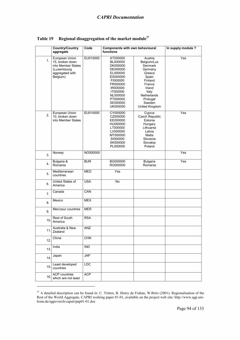
CAPRI Documentation

of 133

Table 19 Regional disaggregation of the market module27

Country/Country aggregate

Code Components with own behavioural functions

In supply module ?

1. European Union 15, broken down into Member States (Luxembourg aggregated with Belgium)

EU015000 AT000000 BL000000 DK000000 DE000000 EL000000 ES000000 FI000000 FR000000 IR000000 IT000000 NL000000 PT000000 SE000000 UK000000

Austria Belgium/Lux

Denmark Germany Greece Spain

Finland France Irland Italy

Netherlands Protugal Sweden

United Kingdom

Yes

2. European Union 10, broken down into Member States

EU010000 CY000000 CZ000000 EE000000 HU000000 LT000000 LV000000 MT000000 SI000000 SK000000 PL000000

Cyprus Czech Republic

Estonia Hungary Lithuania

Latvia Malta

Slovenia Slovakia Poland

Yes

3. Norway NO000000 Yes

4. Bulgaria & Romania

BUR BG000000 RO000000

Bulgaria Romania

Yes

5. Mediterranean countries

MED Yes

6. United States of America

USA No

7. Canada CAN

8. Mexico MEX

9. Mercosur countries MER

10. Rest of South America

RSA

11. Australia & New Zealand

ANZ

12. China CHN

13. India IND

14. Japan JAP

15. Least developed countries

LDC

16. ACP countries which are not least

ACP

27 A detailed description can be found in: C. Tritten, B. Henry de Frahan, W.Britz (2001): Regionalisation of the Rest of the World Aggregate, CAPRI working paper 01-01, available on the project web site: http://www.agp.uni-bonn.de/agpo/rsrch/capstr/pap01-01.doc

CAPRI Documentation

of 133

Country/Country aggregate

Code Components with own behavioural functions

In supply module ?

developed

17. Rest of the world ROW


5.4.2 The approach of the CAPRI market module

Multi-commodity models are as already mentioned above a wide-spread type of agricultural sector models. There are two types of such models, with a somewhat different history. The first type could be labelled ‘template models’, and its first example is Swopsim. Template models use structurally identical equations for each product and region, so that differences between markets are expressed in parameters. Typically, these parameters are either based on literature research, borrowed from other models or simply set by the researcher, and are friendly termed as being ‘synthetic’. Domestic policies in template models are typically expressed by price wedges between market and producer respectively consumer prices, often using the PSE/CSE concept of the OECD. Whereas template models applied in the beginning rather simple functional forms – as constant elasticity double-logs in Swopsim or WATSIM -, since some years flexible functional forms are in vogue, often combined with a calibration algorithm which ensures that the parameter sets are in line with microeconomic theory. The flexible functional forms combined with the calibration algorithm allow for a set of parameters with identical point elasticities to any observed theory consistent behaviour which at the same time recovers quantities at one point of observed prices and income. Ensuring that parameters are in line with profit respectively utility maximisation allows for a welfare analysis of results.

Even if using a different methodology (explicit technology, inclusion of factor markets etc.), it should be mentioned that Computable General Equilibrium models are template models as well in the sense that they use an identical equation structure for all products and regions. Equally, they are in line with microeconomic theory.

The second type of model is older and did emerge from econometrically estimated single-market models linked together, the most prominent example being the FAPRI modelling system. The obvious advantages of that approach are firstly the flexibility to use any functional relation allowing for a good fit ex-post, secondly that the econometrically estimated parameters are rooted in observed behaviour, and thirdly, that the functional form used in simulations is identically to the one used in parameter estimation. The downside is the fact that parameters are typically not estimated subject to regularity conditions and will likely violate some conditions from micro-theory. Consequently, these models are typically not used for welfare analysis. Besides FAPRI, other examples of such models are AgLink at the OECD or the set of models emerging from AgMemod.

The CAPRI market module is a template model using flexible functional forms. The reason is obvious: it is simply impossible to estimate the behavioural equations for about 40 products and 40 countries or country blocks world wide with the resource available to the CAPRI team. Instead, the template approach ensures that the same reasoning is applied across the board, and the flexible functional forms allow for capturing to a large degree region and product specificities. As such, the results from econometric analysis or even complete parameters sets from other models could be mapped into the CAPRI market model.

CAPRI Documentation

of 133

5.4.3 Behavioural equations for supply and feed demand

Supply for each agricultural output i and region r (EU Member States or regional aggregate) is modelled by a supply function derived from a normalised quadratic profit function via the envelope theorem. Supply depends on producer prices ppri normalised with a price index. The price index relates to all those goods – either inputs or outputs – which are not explicitly modelled in the system:

Equation 98 ∑+=j rindex

rjrjiriri p

ppribsassupply

.

,,,,,

Supply curves for the EU Member States, Norway, Bulgaria and Romania are calibrated in each iteration to the last output price vector used in the supply model and the aggregated supply results at Member State level, by shifting the constant terms as. The slope terms bs which capture own and cross-price effects are set in line with profit maximisation, as discussed below. The calibration of the price dependent parameters bs is discussed below.

The system for feed demand is structured identically. However, not producer prices, but raw product prices arm1p determined by the Armington top level aggregator drive feed demand feed, combined with changes in the supply of animal products weighed with feed use factors w:

Equation 99 ∑∑ ⎟⎟⎠

⎞⎜⎜⎝

⎛+=

icali

ii

j rindex

rjrjiriri supply

supplyw

pparm

bfaffeed.

,,,,,

1

Feed use does hence proportionally increase if the supply of meat or milk is increased, and price changes drive substitution inside of the feed mix. It is planned to replace that system in the near future by explicit energy and protein requirement balances linked to energy and protein ‘shadow’ prices which will define then ‘feed incentive’ prices, as it is already realised for the fat and protein balances for dairy products.

As for supply, feed demand curves for the EU Member States, Norway, Bulgaria and Romania are calibrated in each iteration to the last output price vector used in the supply model and the aggregated feed demand at Member State level, by shifting the constant terms af.

5.4.4 Behavioural equations for final demand

The final demand functions are based on the following family of indirect utility functions depending on consumer prices cpri and per capita income y28 where G and F are functions of degree zero in prices (RYAN & WALES 1996) which will be defined below:

Equation 100 )(

),(Fy

GycpriiU−

−=

Using Roy’s identity, the following per capita Marshallian demands PerCap are derived:

28 Per capita income and total expenditure are used as synonyms in the following as the demand is cover all goods and thus exhaust available income.

CAPRI Documentation

of 133

Equation 101 ( )FyG

GiFPerCap i

ii −+=

where the Fi and Gi are the first derivative of F and G versus own prices. The function F is defined as follows:

Equation 102 ii

ir cpridF ∑=

where the di represent the constant terms of the Marshallian demands and can be interpreted as ‘minimum commitment levels’ or consumption quantities independent of prices and income. The term in brackets in the per capita demands in Equation 101 above hence captures the expenditure remaining after the value F of price and income independent commitments d had been subtracted from available income y. The function G, based on the Generalised Leontief formulation:

Equation 103 ∑∑=i j

jiij cpricpribdG

with the derivative of G versus the own price is labelled Gi and defined as:

Equation 104 ∑=i

jiijj cpricpribdGi

Symmetry is guaranteed by a symmetric bd matrix describing the price dependent terms, correct curvature by non-negative the off-diagonal elements of bd, adding up is automatically

given, as Euler’s Law for a homogenous function of degree one ⎟⎟⎠

⎞⎜⎜⎝

⎛∂

∂=∑ ii i

xxxaxa )()( , leads

to:

Equation 105 ( )

yFFyGG

cpridFyG

cpriGcpriPerCap

iii

iii

iii

=+−=

+−= ∑∑

∑

)(

,

and homogeneity is guaranteed by the functional forms as well. The expenditure function can be derived from the indirect utility functions and gives:

Equation 106 ),(

),(ycpriU

GFyUey −==

The function is only semi-flexible as the non-negativity imposed on the off-diagonal elements ensuring correct curvature will exclude Hicksian complementarity, a restriction not deemed important in the light of the product list covered.

Human consumption hcom is simply the sum of population pop multiplied with the per capita demands:

Equation 107 rirri perCappophcom ,, =

CAPRI Documentation

of 133

5.4.5 Behavioural equations for the processing industry

Processing demand for oilseeds is modelled by using behavioural functions derived from a normalised quadratic profit function under the assumption of a fixed I/O relation between seeds, cakes and oils. Consequently, the processing demand proc depends on processing margins procMarg which are differences between the value of the outputs (oil and cake) per unit of oilseed processed and the value of the oilseed inputted:

Equation 108 ∑+=j rindex

rjrjiriri p

procMargbcacproc

.

,,,,,

where the processing margin is defined from the producer prices ppri and crushing coefficients derived from observed supply quantities as:

Equation 109

basrseed

basroilseed

roilseed

basrseed

basrcakseed

rcakseed

rseedseed,r

supplysupply

ppri

supplysupply

ppri

ppriprocMarg

,

,,

,

,,

,

→→

→→

+

+

−=

Finally, output of oils and cakes supply depends on the processed quantities proc of the oilseeds and the crushing coefficients:

Equation 110

basrseed

basrcakoil

rseedoil,r

basrseed

basrcakseed

rseedcake,r

supplysupply

procsupply

supplysupply

procsupply

,

,,

,

,,

→

→

=

=

Special attention is given to the processing stage of dairy products for the EU Member states. First of all, balancing equations for fat and protein ensure that the processed products use up exactly the amount of fat and protein comprised in the raw milk. The fat and protein content cont of raw milk and milk products mlk is based on statistical and engineering information, and kept constant at calibrated base year levels.

Equation 111 ∑=mlk

fpmlkrmlkfpmilkrmilk contsupplycontsupply ,,,"",""

Production of processed dairy products is based on a normalised quadratic function driven by the difference between the dairy product’s market price and the value of its fat and protein content.

Equation 112 ( )

mlk,r mlk,r

mlk, j,r j j,"fat " fat,r j,"prot" prot,r index,rj

supplky am

bm ppri cont ppri cont ppri p

=

+ − −∑

And lastly, prices of raw milk are equal to its fat and protein content valued with fat and protein prices.

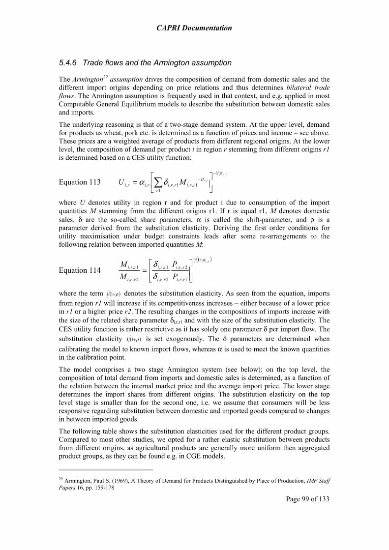
CAPRI Documentation

of 133

5.4.6 Trade flows and the Armington assumption

The Armington29 assumption drives the composition of demand from domestic sales and the different import origins depending on price relations and thus determines bilateral trade flows. The Armington assumption is frequently used in that context, and e.g. applied in most Computable General Equilibrium models to describe the substitution between domestic sales and imports.

The underlying reasoning is that of a two-stage demand system. At the upper level, demand for products as wheat, pork etc. is determined as a function of prices and income – see above. These prices are a weighted average of products from different regional origins. At the lower level, the composition of demand per product i in region r stemming from different origins r1 is determined based on a CES utility function:

Equation 113 ir

ir

rrrirririri MU

,

,

1

11,,1,,,,

ρρδα

−−

⎥⎦

⎤⎢⎣

⎡= ∑

where U denotes utility in region r and for product i due to consumption of the import quantities M stemming from the different origins r1. If r is equal r1, M denotes domestic sales. δ are the so-called share parameters, α is called the shift-parameter, and ρ is a parameter derived from the substitution elasticity. Deriving the first order conditions for utility maximisation under budget constraints leads after some re-arrangements to the following relation between imported quantities M:

Equation 114 ( )ir

rri

rri

rri

rri

rri

rri

PP

MM ,11

1,,

2,,

2,,

1,,

2,,

1,,ρ

δδ

+

⎥⎥⎦

⎤

⎢⎢⎣

⎡=

where the term ( )ρ+11 denotes the substitution elasticity. As seen from the equation, imports from region r1 will increase if its competitiveness increases – either because of a lower price in r1 or a higher price r2. The resulting changes in the compositions of imports increase with the size of the related share parameter δi,r,r1 and with the size of the substitution elasticity. The CES utility function is rather restrictive as it has solely one parameter δ per import flow. The substitution elasticity ( )ρ+11 is set exogenously. The δ parameters are determined when calibrating the model to known import flows, whereas α is used to meet the known quantities in the calibration point.

The model comprises a two stage Armington system (see below): on the top level, the composition of total demand from imports and domestic sales is determined, as a function of the relation between the internal market price and the average import price. The lower stage determines the import shares from different origins. The substitution elasticity on the top level stage is smaller than for the second one, i.e. we assume that consumers will be less responsive regarding substitution between domestic and imported goods compared to changes in between imported goods.

The following table shows the substitution elasticities used for the different product groups. Compared to most other studies, we opted for a rather elastic substitution between products from different origins, as agricultural products are generally more uniform then aggregated product groups, as they can be found e.g. in CGE models.

29 Armington, Paul S. (1969), A Theory of Demand for Products Distinguished by Place of Production, IMF Staff Papers 16, pp. 159-178

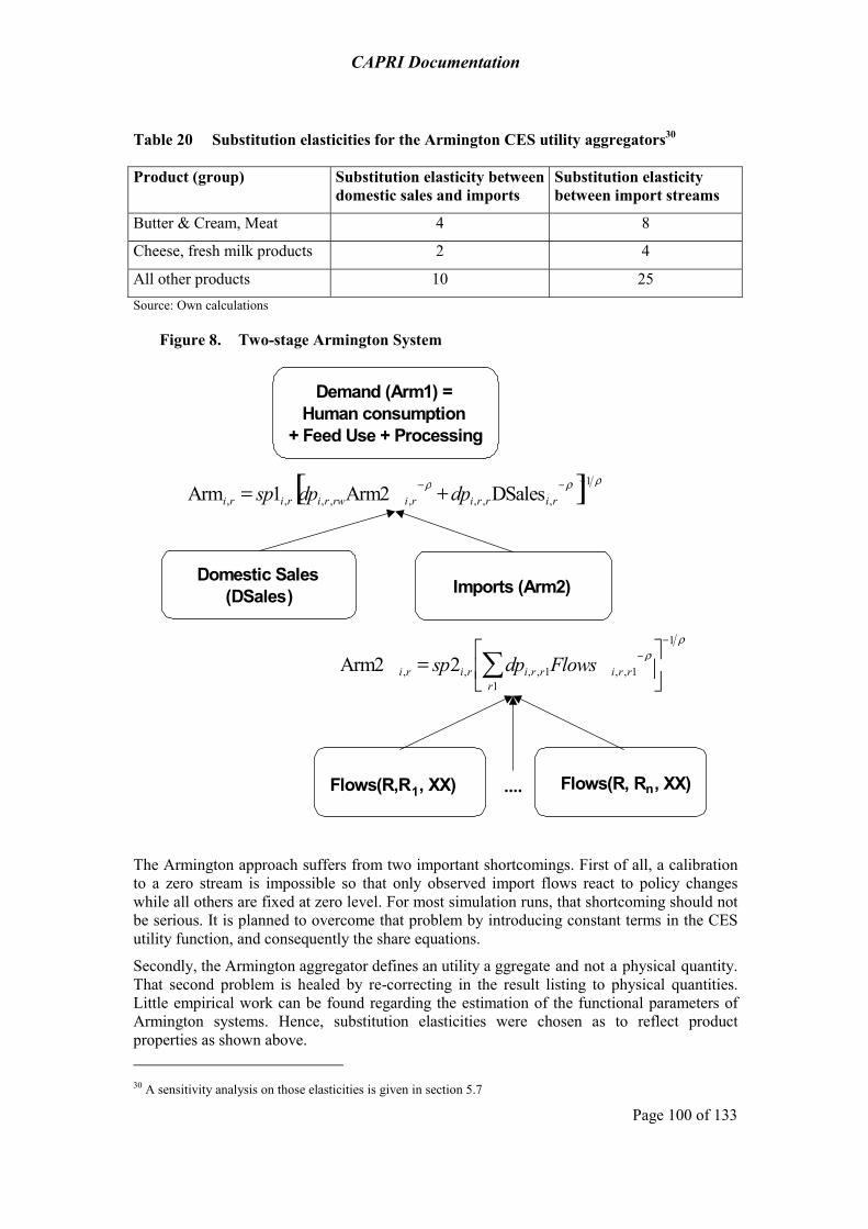
CAPRI Documentation

of 133

Table 20 Substitution elasticities for the Armington CES utility aggregators30

Product (group) Substitution elasticity between domestic sales and imports

Substitution elasticity between import streams

Butter & Cream, Meat 4 8

Cheese, fresh milk products 2 4

All other products 10 25 Source: Own calculations

Figure 8. Two-stage Armington System

Flows(R,R , XX) 1 n ....

ρ ρ

1

1 1 , , 1 , , , , 2 Arm2

− − ⎥ ⎦

⎤ ⎢ ⎣

⎡ = ∑ r

r r i r r i r i r i Flows dp sp

Demand (Arm1) =

Human consumption

+ Feed Use + Processing

Domestic Sales

( DSales ) Imports (Arm2)

[ ] ρ ρ ρ 1

, , , , , , , , DSales Arm2 1 Arm − − − + = r i r r i r i rw r i r i r i dp dp sp

Flows(R, R , XX)

The Armington approach suffers from two important shortcomings. First of all, a calibration to a zero stream is impossible so that only observed import flows react to policy changes while all others are fixed at zero level. For most simulation runs, that shortcoming should not be serious. It is planned to overcome that problem by introducing constant terms in the CES utility function, and consequently the share equations.

Secondly, the Armington aggregator defines an utility a ggregate and not a physical quantity. That second problem is healed by re-correcting in the result listing to physical quantities. Little empirical work can be found regarding the estimation of the functional parameters of Armington systems. Hence, substitution elasticities were chosen as to reflect product properties as shown above. 30 A sensitivity analysis on those elasticities is given in section 5.7

CAPRI Documentation

of 133

5.4.7 Market clearing conditions

All quantities in the model are measured in 1000 metric tons. The quantity balances first state that production must be equal to domestic sales plus export flows plus changes in intervention stocks:

Equation 115 rirr

rririri ischflowsdsalessupply ,1

,1,,, ++= ∑≠

Further on, imports and exports are defined from bilateral trade flows as:

Equation 116 ∑≠

=rr

rriri flowsimports1

1,,,

Equation 117 ∑≠

=rr

rriri flowsexports1

,1,,

Finally, the Armington first stage aggregate arm1, shown in the diagram above, is equal to the domestic consumption elements feed, human consumption and processing:

Equation 118 riririri prochconfeedarm ,,,,1 ++=

5.4.8 Price linkages

All prices in model are expressed as € per metric ton. Import prices imppi,r,r1 from region r1 into region r of product i are determined from market prices pmrk taking into account bilateral ad valorem (tariffa) and specific (tariffs) tariffs minus export subsidies expsub:

Equation 119 ( ) 1,1,,1,,1,1,, 1001 rirrirririrri expsubtariffstariffapmrkimpp −++=

Bilateral tariffs may be endogenous variables if they are determined by a tariff rate quota (TRQ), see below. Equally, export subsidies are endogenous variables.

Producer prices are derived from market prices using direct and indirect PSEs price wedges, except for EU15, EU10 and Bulgaria and Romania. The reader is reminded that for the EU27, the supply model includes a rather detailed description of the different premium schemes of the CAP, so that the EU premiums need not to be modelled as price wedges in the market part.

Equation 120 riririri PSEiPSEdpmrkppri ,,,, ++=

The average prices of imports derived from the Armington second stage aggregate are labelled arm2p and defined as total import value divided by the Armington second stage utility aggregate arm2:

Equation 121 ri

rrrrirri

ri arm

imppflowsparm

,

11,,1,,

, 22

∑≠=

Similarly, the average prices for goods consumed domestically arm1p are a weighted average of the domestic market price pmrk weighted with domestic sales dsales and the Armington second stage utilitiy aggregate arm2 weighted with the average import price arm2p:

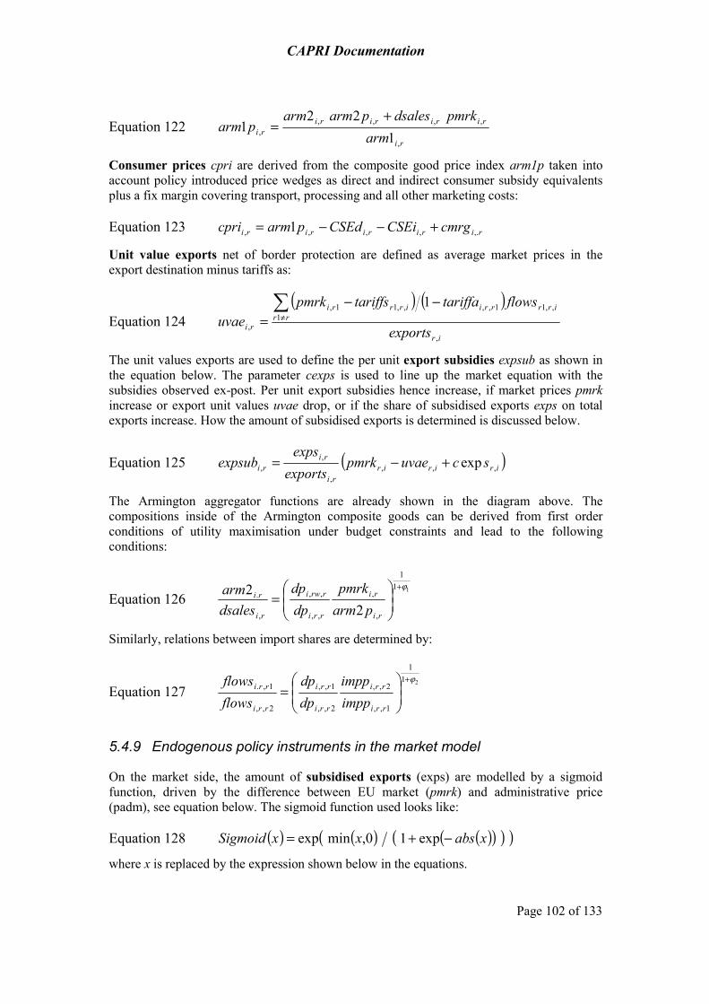
CAPRI Documentation

of 133

Equation 122 ri

ririririri arm

pmrkdsalesparmarmparm

,

,,,,, 1

221

+=

Consumer prices cpri are derived from the composite good price index arm1p taken into account policy introduced price wedges as direct and indirect consumer subsidy equivalents plus a fix margin covering transport, processing and all other marketing costs:

Equation 123 ririririri cmrgCSEiCSEdparmcpri ,.,,,, 1 +−−=

Unit value exports net of border protection are defined as average market prices in the export destination minus tariffs as:

Equation 124 ( ) ( )

ir

rrirrrriirrri

ri exports

flowstariffatariffspmrkuvae

,

1,,11,,,,11,

,

1∑≠

−−=

The unit values exports are used to define the per unit export subsidies expsub as shown in the equation below. The parameter cexps is used to line up the market equation with the subsidies observed ex-post. Per unit export subsidies hence increase, if market prices pmrk increase or export unit values uvae drop, or if the share of subsidised exports exps on total exports increase. How the amount of subsidised exports is determined is discussed below.

Equation 125 ( )iririrri

riri scuvaepmrk

exportsexps

expsub ,,,,

,, exp+−=

The Armington aggregator functions are already shown in the diagram above. The compositions inside of the Armington composite goods can be derived from first order conditions of utility maximisation under budget constraints and lead to the following conditions:

Equation 126 11

1

,

,

,,

,,

,

.

22 ϕ+

⎟⎟⎠

⎞⎜⎜⎝

⎛=

ri

ri

rri

rrwi

ri

ri

parmpmrk

dpdp

dsalesarm

Similarly, relations between import shares are determined by:

Equation 127 21

1

1,,

2,,

2,,

1,,

2,,

1,.ϕ+

⎟⎟⎠

⎞⎜⎜⎝

⎛=

rri

rri

rri

rri

rri

rri

imppimpp

dpdp

flowsflows

5.4.9 Endogenous policy instruments in the market model

On the market side, the amount of subsidised exports (exps) are modelled by a sigmoid function, driven by the difference between EU market (pmrk) and administrative price (padm), see equation below. The sigmoid function used looks like:

Equation 128 ( ) ( ) ( )( )( )( )xabsxxSigmoid −+= exp10,minexp

where x is replaced by the expression shown below in the equations.

CAPRI Documentation

of 133

The response was chosen as steep as technically possible by setting a high value for α, i.e. intervention prices are undercut solely if WTO commitment (QUTE) and the maximum quantity of stock changes are reached.

Equation 129 ( )⎥⎥⎦

⎤

⎢⎢⎣

⎡⎟⎟⎠

⎞⎜⎜⎝

⎛−−= i

Eriri

irEri

ririri PADMpmrk

PADMsigmoidQutEexps1 ,,

,

,,, 1 β

βα

The parameters β are determined based on observed price and quantities of subsidised exports. In order to ensure that subsidised exports do not exceed actual exports, the following smooth approximation is used:

Equation 130 ( ) ⎟⎠⎞

⎜⎝⎛ ++−−+= 20

122012

,,,,21

, 11 ririririri exportsexpsexportsexpsexps

The relation is shown in the figure below.

Figure 9. Modelling of subsidised exports by a logistic function

β PADM

PMrk

EXPSQUTE

PADM

50% QUTE Purchases to intervention stocks intp depend on the probability of the current market price pmrk to undercut the administrative price padm assuming a normally distributed market price with standard deviation stddev and maximal amounts of purchases INTM:

Equation 131 ( )( )ririririri stddevpmrkpadmerrfIntMintp ,,,,, −=

A decrease of the administrative price or an increase of the market price will hence decrease purchases to intervention stocks.

Releases from intervention stocks intd depend on the probability of market prices pmrk to undercut unit value exports uvae, ,multiplied with the current intervention stock size being equal to starting size intk plus intervention purchases intp:

Equation 132 ( ) ( )( )riirririririri stddevpmrkuvaeerrfintpintkintd ,,,,,, γ+−+=

Releases will hence increase if world market price increases or the EU market price drops, and if the size of the intervention stock increases. The parameters γ are determined from ex-post data on prices and intervention stock levels. The change in intervention stocks ints entering the market balance is hence the difference between intervention purchases intp and intervention stock releases intd:

CAPRI Documentation

of 133

Equation 133 ririri intdintpints ,,, −=

5.4.10 Endogenous tariffs under Tariff Rate Quotas

Tariff Rate Quotas (TRQs) establish a two-tier tariff regime: as long as import quantities do not exceed the import quota, the low in-quota tariff is applied. Quantities above the quota are charged with the higher Most-Favoured-Nation (MFN) tariff. CAPRI distinguishes two types of TRQs: such open to all trading partners, and bi-laterally allocated TRQs. Equally, as for all tariffs, TRQs may define ad valorem and/or specific tariffs.

A market under a TRQ mechanism may be in one of the following regimes:

• Quota underfill: the in-quota tariff is applied. The willingness to pay of the consumers is equal to the border price plus the in-quota tariff.

• Quota exactly filled: the in-quota tariff is applied. The willingness to pay of consumers and thus the price paid is somewhere between the border plus the in-quota tariff and the border price plus the MFN tariff. The difference between the price in the market and the border price plus the in-quota tariff establishes a quota rent. Depending on property rights on the quota and the allocation mechanism, the quota rent is shared in different portions by the producers, importing agencies, the domestic marketing chain or the administration. Typically, the quota rent can neither be observed nor is their knowledge about distribution of the rent.

• Quota overfill: the higher MFN-tariff is applied. The quota rent is equal to the difference between the MFN and the in-quota tariff. Again, how the quota rent is distributed to agents is typically not known.

There are a couple of further complications, linked to spatial and commodity aggregation problems. In many cases, TRQs are defined for very specific data qualities, which are more dis-aggregated as the product definition of the model. TRQs for beef may refer e.g. to specific cuts, races or even feeding practises. That typically leads to a situation where both imports covered and not covered by a TRQ mechanism are aggregated in the data base of the model. Consequently, it is not clear, which regime governs the market. Further on, TRQs may be defined for individual countries where the model works on a country block.

Besides the problem of defining the regime ex-post, the relation between the import quantity and the tariff is not differentiable but kinked. Therefore, again a sigmoid function (Figure 9) is applied in the CAPRI market part.

5.4.11 Overview on a regional module inside the market model

The resulting layout of a market for a country (aggregate) in the market module is shown in the following diagram. Due to the Armington assumption, product markets for different regions are linked by import streams and import prices if observed in the base year. Accordingly, no uniform world market price is found in the system.

CAPRI Documentation

of 133

Figure 10. Graphical presentation for one region of a spatial market system

ArmingtonStage 2

Aggregate

ArmingtonStage 1

aggregate

Import Streams

Processing Human consumption Feed Use

Supply

Domestic Sales Export streamsIntervention sales

Export subsidies ?

RegionalPrices

and prices


5.4.12 Basic interaction inside the market module during simulations

As with the supply module, the main difficulty in understanding model reactions is based on the simultaneity of changes occurring after a shock to the model. Cross-price effects and trade relations interlink basically all product markets for all regions. Whereas in the supply model, interactions between products are mostly based on explicit representation of technology (land balances, feed restrictions), such interactions are captured in multi-commodity models in the parameters of the behavioural functions.

Even if the following narrative is simplifying and describing reactions as if they would appear in a kind of natural sequence where they are appear simultaneously in the model, we will nevertheless ‘analyse’ the effect of an increased supply at given prices for one product and one region. Such a shift could e.g. result from the introduction of a subsidy for outputting that product. The increased supply will lead to imbalances in the market clearing equation for that product and that region. These imbalances can only be equilibrated again if supply and demand adjust, which requires price changes. In our example, the price in that region will have to drop to reduce supply. That drop will stimulate feed demand, and to a lesser extent, human consumption. The smaller effect on human consumption has two reasons: firstly, price elasticities for feed demand are typically higher, and secondly, consumer prices are linked with rather high margins to farm gate prices.

The resulting lower price at farm gate increases international competitiveness. Due to the Armington mechanism, consumers around the world will now increase the share of that region in their consumption of that product, and lower their demand from other origins. That will put price pressure in all other regional markets. The pressure will be the higher, the higher the import share of the region with the exogenous increase of supply on the demand of that product. The resulting price pressure will in turn reduce supply and stimulate demand

CAPRI Documentation

of 133

and feed everywhere, and, with reduced prices, offset partially the increased competitiveness of the region where the shock was introduced.

Simultaneously, impacts on market for others products will occur. Depending on the size of the cross price elasticities, demand for other products will drop with falling prices for a substitute. At the same time, reduced prices will stimulate supply of other products. The resulting imbalances will hence force downwards price adjustments in other markets as well.

5.5 Parameter calibration and sources for the behavioural equations

5.5.1 Calibration of the system of supply functions

The supply equation was already introduced in Equation 98. The matrix bs is equal to the Hessian matrix of second derivatives of the normalised profit function to normalised prices and must hence be symmetric by definition. As bs is equal to the first derivative of the supply function against normalised prices, the supply elasticities at the calibration point are defined as:

Equation 134 i

rindex

rj

jiji supplyp

ppri

bs .

,

,, =ε

Homogeneity of supply functions of degree zero is given due to the normalisation with a price index: if all prices and the price index are raised by the same percentage, the supply quantity does not change.

Remains the question of curvature, which is guaranteed if bs is positive definite, ensured by a Cholesky decomposition during the calibration process. The curvature ensures that marginal profits are increased if one or several of the prices are increased, and is one of properties of a profit function derived from micro-theory. The calibration searches for minimal squared deviations between the consistent elasticities and given ones.

The uncalibrated elasticities for the non-EU regions are taken from the World Food Model of the FAO, status 1995. Missing own-supply elasticities are set to 0.5. It is assumed that the elasticity to all remaining products including the inputs is -0.25, if not given.

There are some further restrictions introduced:

• Absolute elasticities are not allowed to be larger than 10.

• Reactions in between cereals and between cereals and meats must be substitutive.

5.5.2 Calibration of the final demand systems

According to the concept of the Supply Utilization Accounts, all processing demand by the food industry is counted as human consumption. Equally, imports of food products are re-converted in primary product equivalents. Human consumption of a primary product in the market model does hence include all processed food products derived from it as pasta, muesli, bread etc. rooting in bread.

As discussed above, the demand system discussed above is homogenous of degree zero in prices and income, and symmetric if bd is symmetric. The somewhat more cumbersome proof that utility is decreasing in prices and increasing in income as long as the matrix bd has only

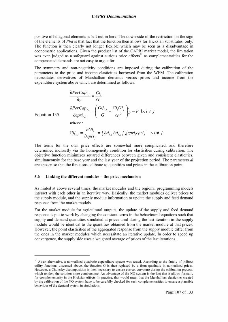
CAPRI Documentation

of 133

positive off-diagonal elements is left out in here. The down-side of the restriction on the sign of the elements of Pbd is that fact that the function then allows for Hicksian substitutes, only. The function is then clearly not longer flexible which may be seen as a disadvantage in econometric applications. Given the product list of the CAPRI market model, the limitation was even judged as a safeguard against curious price effects31 as complementarities for the compensated demands are not easy to argue for.

The symmetry and non-negativity conditions are imposed during the calibration of the parameters to the price and income elasticities borrowed from the WFM. The calibration necessitates derivatives of Marshallian demands versus prices and income from the expenditure system above which are determined as follows:

Equation 135 ( )

jicpricpribdbdcpriGiGij

where

jiFyG

GiGiG

Gijcpri

PerCap

GGi

yPerCap

jijijij

iji

r

jiji

jr

ir

r

iir

≠∧=∂∂

=

≠∧−⎟⎟⎠

⎞⎜⎜⎝

⎛−=

∂∂

=∂

∂

,,21

,

2,

,

,

,

:

The terms for the own price effects are somewhat more complicated, and therefore determined indirectly via the homogeneity condition for elasticities during calibration. The objective function minimizes squared differences between given and consistent elasticities, simultaneously for the base year and the last year of the projection period. The parameters di are chosen so that the functions calibrate to quantities and prices in the calibration point.

5.6 Linking the different modules – the price mechanism

As hinted at above several times, the market modules and the regional programming models interact with each other in an iterative way. Basically, the market modules deliver prices to the supply module, and the supply module information to update the supply and feed demand response from the market models.

For the market module for agricultural outputs, the update of the supply and feed demand response is put to work by changing the constant terms in the behavioural equations such that supply and demand quantities simulated at prices used during the last iteration in the supply module would be identical to the quantities obtained from the market module at that prices. However, the point elasticities of the aggregated response from the supply module differ from the ones in the market modules which necessitate an iterative update. In order to speed up convergence, the supply side uses a weighted average of prices of the last iterations.

31 As an alternative, a normalized quadratic expenditure system was tested. According to the family of indirect utility functions discussed above, the function G is then replaced by a from quadratic in normalized prices. However, a Cholesky decomposition is then necessary to ensure correct curvature during the calibration process, which renders the solution more cumbersome. An advantage of the NQ system is the fact that it allows formally for complementarity in the Hicksian effects. In practice, that would mean that the Marshallian elasticities created by the calibration of the NQ system have to be carefully checked for such complementarities to ensure a plausible behaviour of the demand system in simulations.

CAPRI Documentation

of 133

The first version of CAPRI fixed supply of EU Member States in the market module during iterations. It turned out however, that convergence is achieved faster if supply is price responsive even with differing point elasticities. One of the options discussed is to generate a set of price elasticities from the regional programming models and to calibrate the parameters of the market module to it. However, given the large amount of commodities and regional or even farm type models, these sensitivity analysis would take quite some time.

The interaction between the regional programming models and the young animal module was already explained above. Basically, it is again an iterative update of parameters in a more aggregate model; however, the young animal module comprises models at Member State level which are structurally identical to the regional models. The update thus requires both the definition of a weighted average of the I/O coefficients as well as the application of ideas borrowed from Positive Mathematical Programming to achieve a point calibration. As for marketable outputs, prices for young animals used in any iteration are a weighted average of previous iterations.

5.7 Sensitivity of the CAPRI model to the Armington substitution elasticities A conventional sensitivity analysis consists to run the model using initial Armington elasticities to obtain the baseline, then to rerun it under various elasticity values, all other things held constant, and finally to compare the reference and simulation results. In our sensitivity study, the implementation of this type of analysis shows very small numerical variations on every variable level at less than 0.002 percent. This is the reason why we chose to associate exogenous shocks to the sensitivity analysis.

To perform the sensitivity analysis, we first introduce different sets of Armington substitution elasticities in the model. Then, we introduce an exogenous shock by changing, for example, the policy parameters or the shift factors in the supply equations. Finally, we compare the reactions of endogenous variables (price, production, domestic sales, imports, exports) for different sets of elasticities as show in Figure 11.

Three exogenous shocks, associated to the sensitivity analysis, are thus implemented: (i) a 20% decrease in supply, (ii) a 10% decrease in subsidized exports, (iii) an increase in tariff rate quotas. For each shock, the simulation related to the initial Armington elasticities, i.e., scenario 3, is used as the baseline. Its results are compared to those of the sensitivity runs.

The sets of substitution elasticities are obtained by shifting the initial value of these elasticities to more or less 70 percent. The use of the same percentage change - between the baseline and the other sensitivity runs - allows to evaluate the degree of symmetry in the sensitivity. Lower values for elasticities imply a decrease of preference and thus a greater difficulty in substituting between demand origins, whereas higher values for elasticities imply an increase of preference and, thus, a greater ease in substituting between demand origins.

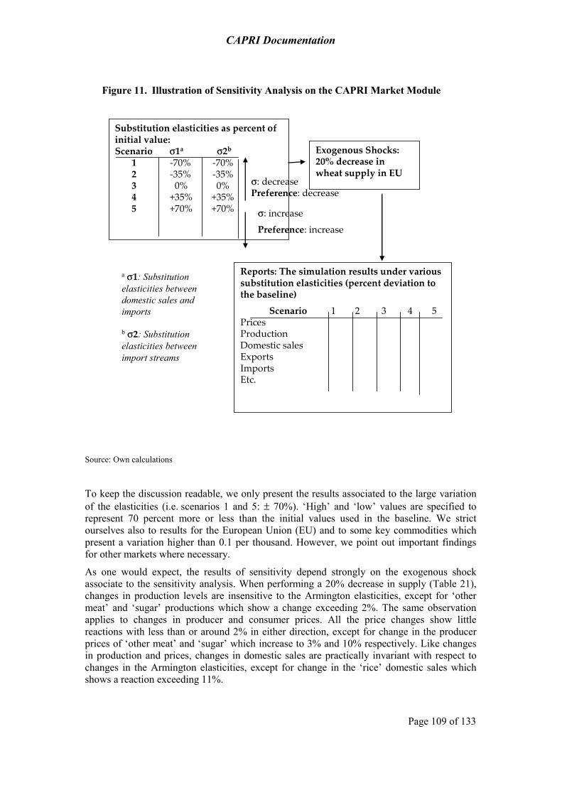
CAPRI Documentation

of 133

Figure 11. Illustration of Sensitivity Analysis on the CAPRI Market Module

σ: decreasePreference: decrease

σ: increase

Preference: increase

Substitution elasticities as percent of initial value:Scenario σ1a σ2b

1 -70% -70%2 -35% -35%3 0% 0%4 +35% +35%5 +70% +70%

Reports: The simulation results under various substitution elasticities (percent deviation to the baseline)

Scenario 1 2 3 4 5 Prices ProductionDomestic salesExportsImportsEtc.

a σ1: Substitution elasticities between domestic sales and imports

b σ2: Substitution elasticities between import streams

Exogenous Shocks:20% decrease in wheat supply in EU


To keep the discussion readable, we only present the results associated to the large variation of the elasticities (i.e. scenarios 1 and 5: ± 70%). ‘High’ and ‘low’ values are specified to represent 70 percent more or less than the initial values used in the baseline. We strict ourselves also to results for the European Union (EU) and to some key commodities which present a variation higher than 0.1 per thousand. However, we point out important findings for other markets where necessary.

As one would expect, the results of sensitivity depend strongly on the exogenous shock associate to the sensitivity analysis. When performing a 20% decrease in supply (Table 21), changes in production levels are insensitive to the Armington elasticities, except for ‘other meat’ and ‘sugar’ productions which show a change exceeding 2%. The same observation applies to changes in producer and consumer prices. All the price changes show little reactions with less than or around 2% in either direction, except for change in the producer prices of ‘other meat’ and ‘sugar’ which increase to 3% and 10% respectively. Like changes in production and prices, changes in domestic sales are practically invariant with respect to changes in the Armington elasticities, except for change in the ‘rice’ domestic sales which shows a reaction exceeding 11%.

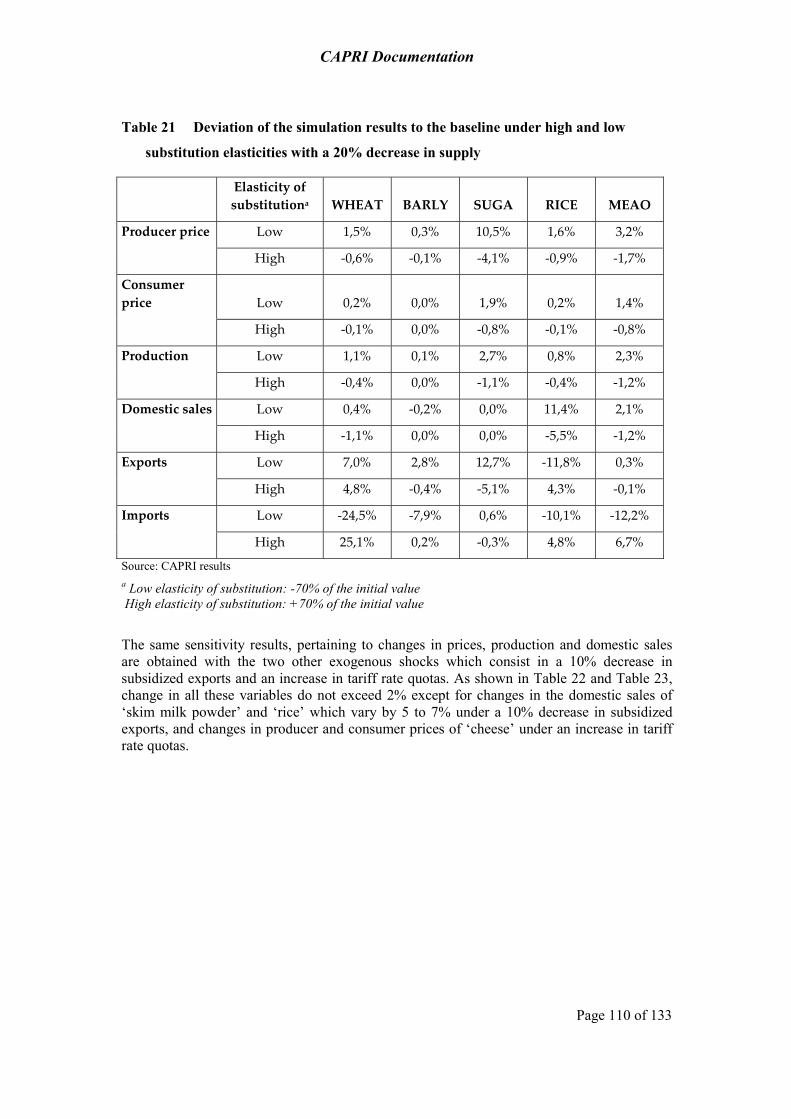
CAPRI Documentation

of 133

Table 21 Deviation of the simulation results to the baseline under high and low

substitution elasticities with a 20% decrease in supply

Elasticity of substitutiona WHEAT BARLY SUGA RICE MEAO

Producer price Low 1,5% 0,3% 10,5% 1,6% 3,2%

High -0,6% -0,1% -4,1% -0,9% -1,7%

Consumer price Low 0,2% 0,0% 1,9% 0,2% 1,4%

High -0,1% 0,0% -0,8% -0,1% -0,8%

Production Low 1,1% 0,1% 2,7% 0,8% 2,3%

High -0,4% 0,0% -1,1% -0,4% -1,2%

Domestic sales Low 0,4% -0,2% 0,0% 11,4% 2,1%

High -1,1% 0,0% 0,0% -5,5% -1,2%

Exports Low 7,0% 2,8% 12,7% -11,8% 0,3%

High 4,8% -0,4% -5,1% 4,3% -0,1%

Imports Low -24,5% -7,9% 0,6% -10,1% -12,2%

High 25,1% 0,2% -0,3% 4,8% 6,7%

Source: CAPRI results a Low elasticity of substitution: -70% of the initial value High elasticity of substitution: +70% of the initial value

The same sensitivity results, pertaining to changes in prices, production and domestic sales are obtained with the two other exogenous shocks which consist in a 10% decrease in subsidized exports and an increase in tariff rate quotas. As shown in Table 22 and Table 23, change in all these variables do not exceed 2% except for changes in the domestic sales of ‘skim milk powder’ and ‘rice’ which vary by 5 to 7% under a 10% decrease in subsidized exports, and changes in producer and consumer prices of ‘cheese’ under an increase in tariff rate quotas.

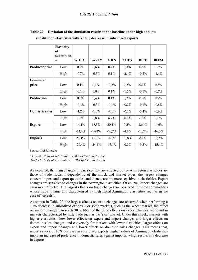
CAPRI Documentation

of 133


substitution elasticities with a 10% decrease in subsidized exports

Elasticity of substitution WHEAT BARLY MILS CHES RICE BEFM

Producer price Low 0,9% 0,6% 0,2% 0,3% 0,8% 1,6%

High -0,7% -0,5% 0,1% -2,4% -0,3% -1,4%

Consumer price Low 0,1% 0,1% -0,2% 0,2% 0,1% 0,8%

High -0,1% 0,0% 0,1% -1,5% -0,1% -0,7%

Production Low 0,5% 0,4% 0,1% 0,2% 0,3% 0,9%

High -0,4% -0,3% -0,1% -0,7% -0,1% -0,8%

Domestic sales Low -1,2% -1,0% -7,1% -0,2% -5,4% -0,6%

High 1,3% 0,8% 6,7% -0,5% 6,3% 1,0%

Exports Low 14,4% 18,5% 20,1% 7,2% 22,4% 14,6%

High -14,4% -16,4% -18,7% -4,1% -18,7% -16,5%

Imports Low 21,4% 16,1% 14,0% 13,8% 8,1% 10,2%

High -29,4% -24,4% -13,1% -0,9% -9,3% -15,4%

Source: CAPRI results a Low elasticity of substitution: -70% of the initial value High elasticity of substitution: +70% of the initial value

As expected, the main changes in variables that are affected by the Armington elasticities are those of trade flows. Independently of the shock and market types, the largest changes concern import and export quantities and, hence, are the more sensitive to elasticities. Export changes are sensitive to changes in the Armington elasticities. Of course, import changes are even more affected. The largest effects on trade changes are observed for most commodities whose trade is large and characterised by high initial Armington elasticities such as in the case of ‘cereals’.

As shown in Table 22, the largest effects on trade changes are observed when performing a 10% decrease in subsidized exports. For some markets, such as the wheat market, the effect on import changes can reach 30%. Most of the large effects on export changes are found in markets characterized by little trade such as the ‘rice’ market. Under this shock, markets with higher elasticities show lower effects on export and import changes and larger effects on domestic sales changes, and conversely for markets with lower elasticities, larger effects on export and import changes and lower effects on domestic sales changes. This means that, under a shock of 10% decrease in subsidized exports, higher values of Armington elasticities imply an increase of preference in domestic sales against imports, which results in a decrease in exports.

CAPRI Documentation

of 133


substitution elasticities with an increase in tariff rate quotasa

Elasticity of substitutionb BARLY MILS CHES BTCR SUGA

Producer price Low 0,0% 0,1% -5,3% 2,8% 0,0%

High 0,0% 0,0% 0,8% -1,5% 0,0%

Consumer price Low 0,0% -0,6% -3,2% 1,6% 0,0%

High 0,0% 0,1% 0,5% -0,9% 0,0%

Production Low 0,0% 0,1% -0,6% 0,5% 0,0%

High 0,0% -0,1% 0,1% -0,2% 0,0%

Domestic sales Low -0,1% 0,5% -1,1% 0,6% 0,0%

High 0,0% -0,1% 0,2% -0,2% 0,0%

Exports Low 0,1% -0,7% 6,7% 19,9% 0,0%

High 0,0% 0,0% -0,5% -23,7% 0,0%

Imports Low 0,8% -0,4% -1,2% -15,7% 0,0%

High -0,3% 0,1% 0,3% 5,0% 0,0%

Source: CAPRI results a The percentage of the increase in the TRQ applied for each commodity depends on the imports and the tariff rate quotas in the base years b Low elasticity of substitution: -70% of the initial value High elasticity of substitution: +70% of the initial value

As shown in Table 23, when performing an increase on tariff rate quotas (TRQ), effects on the changes in most of the variables are not sensitive to the Armington elasticities. It means that effects of the TRQ on model outcomes under different sets of Armington elasticities are marginal.

With respect to symmetry in the opposite change in Armington elasticities, we observe that the percentages of change in variable levels versus their initial values do not show much symmetry. For most of the variables and commodities, changes are larger in the lower substitution elasticities (-70%) than in the higher substitution elasticities (+70%), as expected since the relative change in parameters is larger in the former than in the latter. Exceptions appear on changes in imports under the assumption of a decrease in subsidized exports, which react conversely, i.e. changes are less in the lower substitution elasticities than in the higher substitution elasticities (Table 22).

In sum, all the effects on the changes in variable levels remain low compared to the changes applied on the Armington elasticities (± 70%). The model outcomes are thus comparatively insensitive to the actual magnitude of the Armington elasticities.

CAPRI Documentation

of 133

6 Farm Type Programming Model: a FADN-based approach

6.1 The CAPRI farm type approach

The main aims linked to the introduction of farm types in the system is to ameliorate the analysis of agricultural policies linked to structural variables as farm size or stocking density, improve the reliability of environmental indicators and allow for income analysis at farm type level. In other words, the introduction of data for single farms from the FADN data base reduces the aggregation bias of the model at regional level.

The farm group models could be classified by a number of indicators like the economic importance (farms with high agricultural income against those with lower ones), environmental impact (classic against ecological farming) and many others. The standard grouping in FADN is based on specialisation (e.g. specialised in pig production), which might be supported on the following arguments:

− First of all, the resulting groups are already clearly defined according to official European documents (Commission Decision 2003/369/EC) and results obtained can be easily compared to other studies,

− secondly, the grouping is based on standard gross margins, reducing the stochastic impact of weather or price changes on the grouping for single years, and

− as a third point, it can be argued that environmental impacts are often linked to farm specialisation.

But even with the farm typology according to European standards applied, a number of issues need to be addressed for its application in CAPRI:

(1) Number of farm groups defined for each region. Clearly, the amount of detail increases with the number of farm types, in line with computing time and management costs to handle the additional information. Due to such resource and technical restrictions, in CAPRI it was decided to choose not more than five farm types (the most representative) plus a mixed remaining group representing all other farms for the modelling system (and allowing consistent aggregation of regional data).

(2) Level of typology: For simplicity and a better comparison to FADN, we use the same three digit typology as defined in FADN. Consequently, 50 different types of specialisation can be found in CAPRI (see table 24).

The following diagram shows the relation between the FADN data base and the elements of the CAPRI data processor.

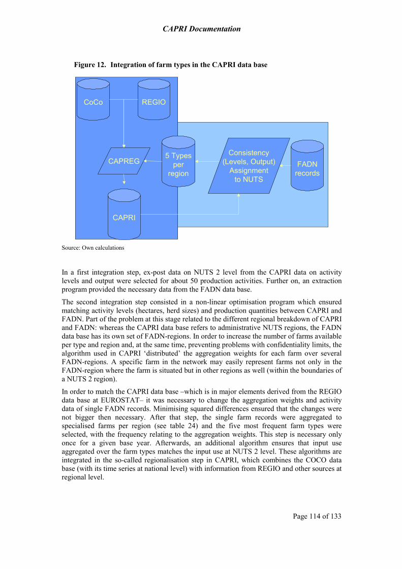
CAPRI Documentation

of 133

Figure 12. Integration of farm types in the CAPRI data base

CoCo REGIO

CAPREG5 Types

perregion

FADNrecords

CAPRI

Consistency(Levels, Output)

Assignmentto NUTS


In a first integration step, ex-post data on NUTS 2 level from the CAPRI data on activity levels and output were selected for about 50 production activities. Further on, an extraction program provided the necessary data from the FADN data base.

The second integration step consisted in a non-linear optimisation program which ensured matching activity levels (hectares, herd sizes) and production quantities between CAPRI and FADN. Part of the problem at this stage related to the different regional breakdown of CAPRI and FADN: whereas the CAPRI data base refers to administrative NUTS regions, the FADN data base has its own set of FADN-regions. In order to increase the number of farms available per type and region and, at the same time, preventing problems with confidentiality limits, the algorithm used in CAPRI ‘distributed’ the aggregation weights for each farm over several FADN-regions. A specific farm in the network may easily represent farms not only in the FADN-region where the farm is situated but in other regions as well (within the boundaries of a NUTS 2 region).

In order to match the CAPRI data base –which is in major elements derived from the REGIO data base at EUROSTAT– it was necessary to change the aggregation weights and activity data of single FADN records. Minimising squared differences ensured that the changes were not bigger then necessary. After that step, the single farm records were aggregated to specialised farms per region (see table 24) and the five most frequent farm types were selected, with the frequency relating to the aggregation weights. This step is necessary only once for a given base year. Afterwards, an additional algorithm ensures that input use aggregated over the farm types matches the input use at NUTS 2 level. These algorithms are integrated in the so-called regionalisation step in CAPRI, which combines the COCO data base (with its time series at national level) with information from REGIO and other sources at regional level.

CAPRI Documentation

of 133

Table 24 Farm types found in the system

131 Specialist COP (other than rice) 132 Specialist rice 133 COP and rice combined 141 Specialist root crops 142 Cereals and root crops combined 143 Specialist field vegetables 144 Various field crops 201 Specialist market garden vegetables 202 Specialist flowers and ornamentals 203 General market garden cropping 311 Quality wine 312 Wine other than quality 313 Quality & other wine combined 314 Vineyards for various types of production 321 Specialist fruit (other than citrus) 322 Citrus fruits 323 Fruits & citrus fruits combined 330 Olives 340 Various permanent crops combined 411 Milk 412 Milk & cattle rearing 421 Cattle rearing 422 Cattle fattening 431 Dairying with rearing & fattening 432 Rearing & fattening with dairying 441 Sheep 442 Sheep & cattle combined 443 Goats 444 Various grazing livestock 501 Specialist pigs 502 Specialist poultry 503 Various garnitures combined 601 Market gardening & permanent crops 602 Field crops & market gardening 603 Field crops & vineyards 604 Field crops & permanent crops 605 Mixed cropping-mainly field crops 606 Mixed cropping-mainly market gardening or permanent crops 711 Mixed livestock-mainly dairying 712 Mixed livestock-mainly non-dairy grazing 721 Mixed livestock-granivores & dairying 722 Mixed livestock-granivores & non-dairy grazing 723 Mixed livestock-granivores with various livestock 811 Field crops & dairying 812 Dairying & field crops 813 Field crops & non-dairy grazing 814 Non-dairy grazing & field crops 821 Field crops & granivores 822 Permanent crops & grazing livestock 823 Various mixed crops and livestock 999 Rest

Source: FADN (http://europa.eu.int/comm/agriculture/rica/index_en.cfm).

CAPRI Documentation

of 133

In the CAPRI modelling system, farm types are treated technically as a further breakdown inside NUTS 2 regions (pseudo-regions): the activity levels in each farm type feature own input and output coefficients and are independently optimised for maximal profits (template approach of the CAPRI supply module). After a model run, the farm type results are aggregated to NUTS 2, Member State and EU level.

It should be noted that the relation between NUTS 2 and Member States is geographical; the disaggregation thus provides localised effects in space. Farm type data however cannot be linked to specific locations in the NUTS 2 regions, even if they break down consistently output, in physical and valued terms, activity levels, and economic and environmental indicators. An improvement in that respect would require a complete link with a Geographical Information System plus intensive economic analysis to create mapping algorithms between spatial specifics (soil types, local climate, slope, altitude ..), production program and farm specialisation. Some work in this direction is being undertaken in CAPRI-Dynaspat and, possibly, in SEAMLESS.

Figure 13 shows the coding scheme. Member States are labelled with two character codes according to EUROSTAT standards (AT for Austria, BL for Belgium and Luxembourg, DK for Denmark, DE for Germany, ...). Regions inside a Member State receive a 3-digit code (first position: NUTS 1 level, second: NUTS 2 level, third: NUS III level) following the EUROSTAT NUTS classification scheme. The farm types are labelled with alphanumerical three-digits code as well, where the ‘000’ refers to the regional level.

Figure 13. Aggregation from farm types to NUTS 2 and Member State

Member StateMS000000

MS110000

MS120000

MS220000MS210000

MS120131

MS120141

MS120412MS120811

MS120812

MS120999


Moreover, the system aggregates across regions all farms of the same specialisation, allowing for the analysis of effects for farms of a certain specialisation across Europe. In order to add

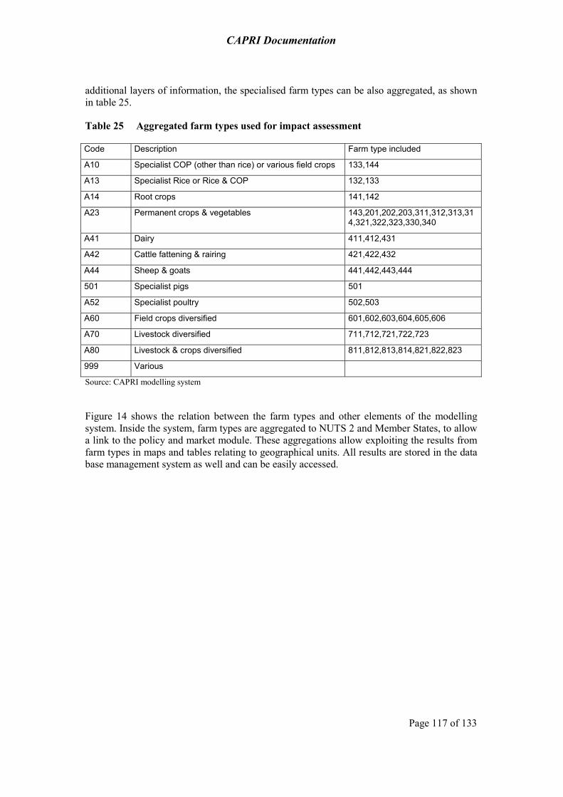
CAPRI Documentation

of 133

additional layers of information, the specialised farm types can be also aggregated, as shown in table 25.

Table 25 Aggregated farm types used for impact assessment

Code Description Farm type included

A10 Specialist COP (other than rice) or various field crops 133,144

A13 Specialist Rice or Rice & COP 132,133

A14 Root crops 141,142

A23 Permanent crops & vegetables 143,201,202,203,311,312,313,314,321,322,323,330,340

A41 Dairy 411,412,431

A42 Cattle fattening & rairing 421,422,432

A44 Sheep & goats 441,442,443,444

501 Specialist pigs 501

A52 Specialist poultry 502,503

A60 Field crops diversified 601,602,603,604,605,606

A70 Livestock diversified 711,712,721,722,723

A80 Livestock & crops diversified 811,812,813,814,821,822,823

999 Various


Figure 14 shows the relation between the farm types and other elements of the modelling system. Inside the system, farm types are aggregated to NUTS 2 and Member States, to allow a link to the policy and market module. These aggregations allow exploiting the results from farm types in maps and tables relating to geographical units. All results are stored in the data base management system as well and can be easily accessed.

CAPRI Documentation

of 133

Figure 14. Integration of farm types in the CAPRI modelling system

CAPRIRegionalised

Data Base

CAPRIModellingSystem

Farm types

AggregationNUTS II

AggregationMS,EU

CAPRIResult

Data Base

Mappingtool

HTMLtables

DAOUT

EXCELetc.


Figure 15 shows the dominant farm types per country. For reasons of survey research the farm types mentioned in table 25 are further combined. It clearly shows that dairy is a dominant farm type in north of Europe. An exception is Denmark where specialised COP, livestock and crops diversified and specialised pigs and poultry are the dominant farm types. Cattle fattening, rearing, sheep and goats are the dominant farm types in Ireland and United Kingdom. In the south of Europe, Portugal, Spain, Italy and Greece, permanent crops and vegetables is the dominant farm type. Also in France and to a lesser extent in Belgium/Luxembourg and the Netherlands, this farm type is relatively important. The heterogeneity of farm types seems to be quite big in France (different farm types have about the same weight) and small in Ireland.

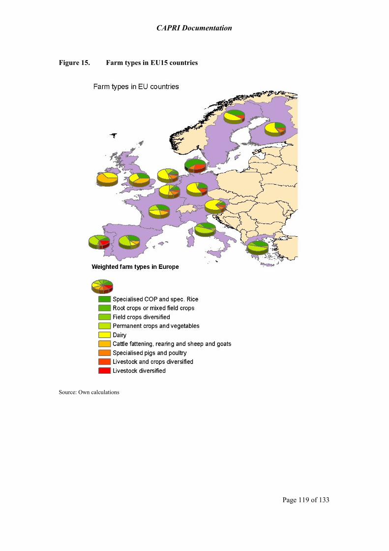
CAPRI Documentation

of 133

Figure 15. Farm types in EU15 countries


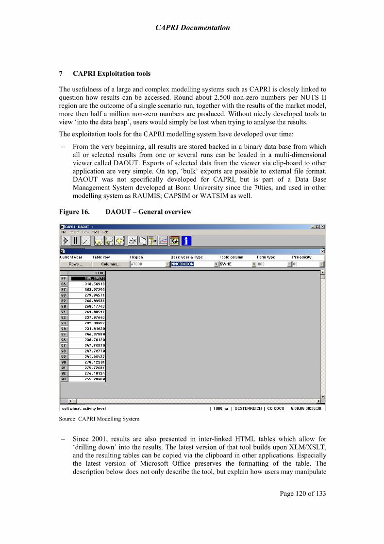
CAPRI Documentation

of 133

7 CAPRI Exploitation tools

The usefulness of a large and complex modelling systems such as CAPRI is closely linked to question how results can be accessed. Round about 2.500 non-zero numbers per NUTS II region are the outcome of a single scenario run, together with the results of the market model, more then half a million non-zero numbers are produced. Without nicely developed tools to view ‘into the data heap’, users would simply be lost when trying to analyse the results.

The exploitation tools for the CAPRI modelling system have developed over time:

− From the very beginning, all results are stored backed in a binary data base from which all or selected results from one or several runs can be loaded in a multi-dimensional viewer called DAOUT. Exports of selected data from the viewer via clip-board to other application are very simple. On top, ‘bulk’ exports are possible to external file format. DAOUT was not specifically developed for CAPRI, but is part of a Data Base Management System developed at Bonn University since the 70ties, and used in other modelling system as RAUMIS; CAPSIM or WATSIM as well.

Figure 16. DAOUT – General overview


− Since 2001, results are also presented in inter-linked HTML tables which allow for ‘drilling down’ into the results. The latest version of that tool builds upon XLM/XSLT, and the resulting tables can be copied via the clipboard in other applications. Especially the latest version of Microsoft Office preserves the formatting of the table. The description below does not only describe the tool, but explain how users may manipulate

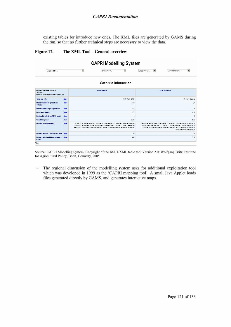
CAPRI Documentation

of 133

existing tables for introduce new ones. The XML files are generated by GAMS during the run, so that no further technical steps are necessary to view the data.

Figure 17. The XML Tool – General overview

Source: CAPRI Modelling System; Copyright of the XSLT/XML table tool Version 2.0: Wolfgang Britz, Institute for Agricultural Policy, Bonn, Germany, 2005

− The regional dimension of the modelling system asks for additional exploitation tool which was developed in 1999 as the ‘CAPRI mapping tool’. A small Java Applet loads files generated directly by GAMS, and generates interactive maps.

CAPRI Documentation

of 133

Figure 18. The mapping tool – general design


Some of these exploitation tools will be ‘exported’ in its current form or with slight modifications. Further technical details are provided in the CAPRI web site.

CAPRI Documentation

of 133

References

Adenaeuer, M.; Louhichi, K.; de Frahan, B.H., Witzke, H.P. (2004). Impacts of the ‘Everything but Arms’ initiative on the EU sugar sub-sector. Selected paper prepared for presentation at the International Conference on Policy Modelling (EcoMod2004), June 30 - July 2, Paris

Armington, P. S., 1969. A Theory of Demand for Products Distinguished by Place of Production. IMF Staff Papers 16, 159-178.

Britz, W., Henrichsmeyer, W., Wieck, C., Perez, I., 2002. Impact analysis of the European Commission’s proposal under the mid-term review of the Common Agricultural Policy (using the CAPRI model). Final Report 75p, University of Bonn.

Britz, W., Pérez, I. and Wieck, C. (2003) Mid-Term Review Proposal Impact Analysis with the CAPRI Modelling System, in: Mid-Term Review of the Common Agricultural Policy - July 2002 Proposals Impact Analyses, European Commission, Directorate-General for Agriculture, pp.111-140, Brussels.

Britz, W., Wieck, C. and Jansson, T. (2002) National Framework of the CAPRI Data base: The COCO-Module, Working paper 02-04, CAPRI Project, Institute for Agricultural Policy, Bonn.

EUROSTAT, 1995. ‘REGIO, Regional data bank, Description of content’.

Henrichsmeyer, W., Lampe, M., Mollmann, C., 2001. Simulating the impact of further trade liberalisation on agricultural world markets using the improved World Agricultural Trade Simulation Model WATSIM. Final Report 76p, University of Bonn.

IPCC (1997) Revised 1996 IPCC Guidelines for National Greenhouse Gas Inventories, Workbook and Reference Manual, Paris.

IPCC (2000) Good Practice Guidance and Uncertainty Management in National Greenhouse gas Inventories, Japan.

Perez I. (2005) Greenhouse Gases: Inventories, Abatement Costs and Markets for Emission Permits in European Agriculture - A Modelling Approach, Doctoral Thesis, 165 pp.

Ryan, D.L., Wales, T.J., 1996. ‘Flexible and Semiflexible Consumer Demands with Quadratic Engel Curves’. Discussion paper No. 96-30, Department of Economics, University of British Columbia, Vancouver Canada.

Undersander, D., Mertens, D. and Thiex, N. (1993) Forage Analyses Procedures, National Forage Testing Association (NFTA), Omaha.

Wolf, W., 1995. ‘SPEL system, Methodological documentation (Rev. 1), Vol. 1: Basics, BS, SFSS’, Eurostat Luxembourg.

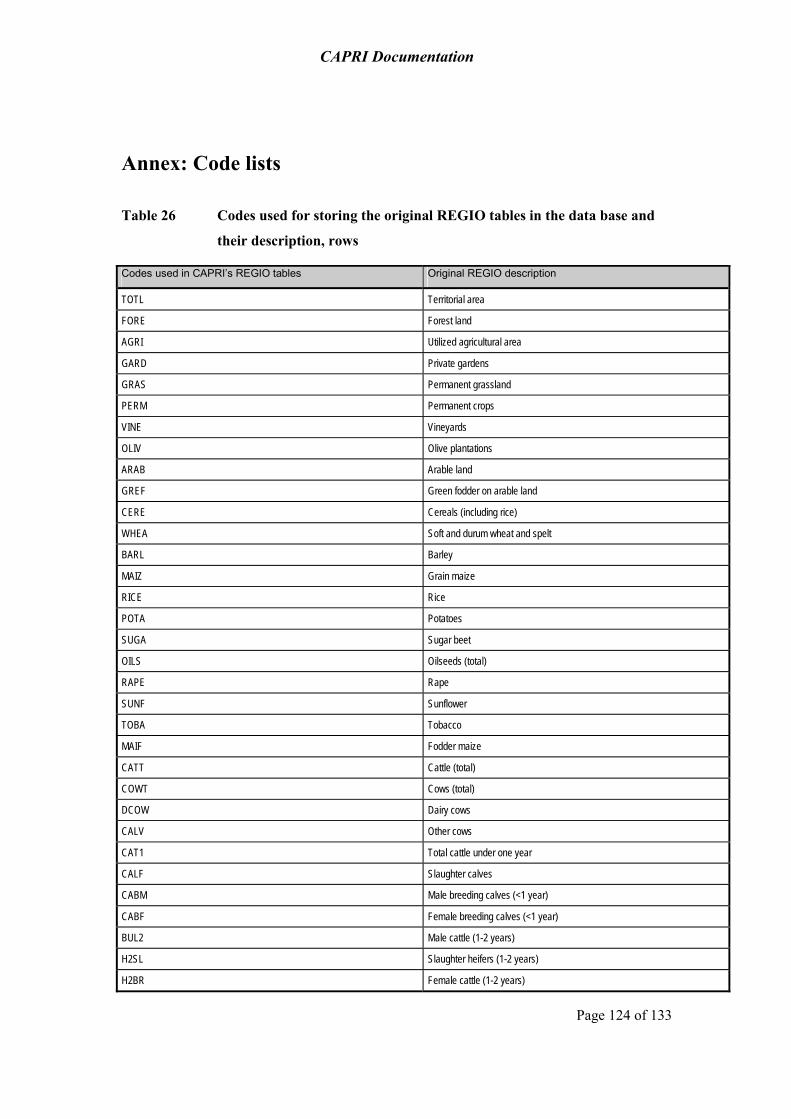
CAPRI Documentation

of 133

Annex: Code lists

Table 26 Codes used for storing the original REGIO tables in the data base and

their description, rows

Codes used in CAPRI’s REGIO tables Original REGIO description

TOTL Territorial area

FORE Forest land

AGRI Utilized agricultural area

GARD Private gardens

GRAS Permanent grassland

PERM Permanent crops

VINE Vineyards

OLIV Olive plantations

ARAB Arable land

GREF Green fodder on arable land

CERE Cereals (including rice)

WHEA Soft and durum wheat and spelt

BARL Barley

MAIZ Grain maize

RICE Rice

POTA Potatoes

SUGA Sugar beet

OILS Oilseeds (total)

RAPE Rape

SUNF Sunflower

TOBA Tobacco

MAIF Fodder maize

CATT Cattle (total)

COWT Cows (total)

DCOW Dairy cows

CALV Other cows

CAT1 Total cattle under one year

CALF Slaughter calves

CABM Male breeding calves (<1 year)

CABF Female breeding calves (<1 year)

BUL2 Male cattle (1-2 years)

H2SL Slaughter heifers (1-2 years)

H2BR Female cattle (1-2 years)

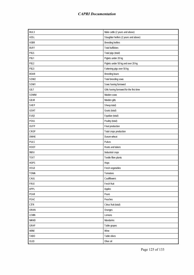
CAPRI Documentation

of 133

BUL3 Male cattle (2 years and above)

H3SL Slaughter heifers (2 years and above)

H3BR Breeding heifers

BUFF Total buffaloes

PIGS Total pigs (total)

PIG1 Piglets under 20 kg

PIG2 Piglets under 50 kg and over 20 kg

PIG3 Fattening pigs over 50 kg

BOAR Breeding boars

SOW2 Total breeding sows

SOW1 Sows having farrowed

GILT Gilts having farrowed for the first time

SOWM Maiden sows

GILM Maiden gilts

SHEP Sheep total)

GOAT Goats (total)

EUQI Equidae (total)

POUL Poultry (total)

OUTP Final production

CROP Total crops production

DWHE Durum wheat

PULS Pulses

ROOT Roots and tubers

INDU Industrial crops

TEXT Textile fibre plants

HOPS Hops

VEGE Fresh vegetables

TOMA Tomatoes

CAUL Cauliflowers

FRUI Fresh fruit

APPL Apples

PEAR Pears

PEAC Peaches

CITR Citrus fruit (total)

ORAN Oranges

LEMN Lemons

MAND Mandarins

GRAP Table grapes

WINE Wine

TABO Table olives

OLIO Olive oil

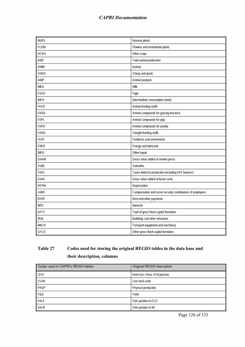
CAPRI Documentation

of 133

NURS Nursery plants

FLOW Flowers and ornamental plants

OCRO Other crops

ANIT Total animal production

ANIM Animal

SHGO Sheep and goats

ANIP Animal products

MILK Milk

EGGS Eggs

INPU Intermediate consumption (total)

FEED Animal feeding stuffs

FDGR Animal compounds for grazing livestock

FDPI Animal compounds for pigs

FDPO Animal compounds for poultry

FODD Straight feeding stuffs

FERT Fertilizers and enrichments

ENER Energy and lubricants

INPO Other inputs

GVAM Gross value added at market prices

SUBS Subsidies

TAXS Taxes linked to production (including VAT balance)

GVAF Gross value added at factor costs

DEPM Depreciation

LABO Compensation and social security contributions of employees

RENT Rent and other payments

INTE Interests

GFCF Total of gross fixed capital formation

BUIL Buildings and other structures

MACH Transport equipment and machinery

GFCO Other gross fixed capital formation

Table 27 Codes used for storing the original REGIO tables in the data base and

their description, columns

Codes used in CAPRI’s REGIO tables Original REGIO description

LEVL Herd size / Area / # of persons

LSUN Live stock units

PROP Physical production

YILD Yield

VALE EAA position in ECU

VALN EAA position in NC

CAPRI Documentation

of 133

Table 28 Connection between CAPRI and REGIO crop areas, crop production

and herd sizes

SPEL-code REGIO-code REGIO-code REGIO-code REGIO-code Description of SPEL activity

SWHE WHEA CERE ARAB Soft wheat

DWHE WHEA CERE ARAB Durum wheat

RYE CERE ARAB Rye

BARL BARL CERE ARAB Barley

OATS CERE ARAB Oats

MAIZ MAIZ CERE ARAB Maize

OCER CERE ARAB Other cereals (excl. rice)

PARI RICE CERE ARAB Paddy rice

PULS ARAB Pulses

POTA POTA ARAB Potatoes

SUGB SUGA ARAB Sugar beet

RAPE RAPE OILS ARAB Rape and turnip rape

SUNF SUNF OILS ARAB Sunflower seed

SOYA OILS ARAB Soya beans

OLIV OLIV PERM Olives for oil

OOIL OILS ARAB Other oil seeds and oleaginous fruits

FLAX ARAB Flax and hemp *** (faser) ***

TOBA TOBA ARAB Tobacco, unmanufactured, incl. dried

OIND ARAB Other industrial crops

CAUL ARAB Cauliflowers

TOMA ARAB Tomatoes

OVEG ARAB Other vegetables

APPL PERM Apples, pears and peaches

OFRU PERM Other fresh fruits

CITR PERM Citrus fruits

TAGR VINE PERM Table grapes

TABO OLIV PERM Table olives

TWIN VINE PERM Table wine

OWIN VINE PERM Other wine

NURS PERM Nursery plants

FLOW ARAB Flowers,ornamental plants, etc.

OCRO ARAB Other final crop products

MILK DCOW Dairy cows

BEEF BUL2 BUL3 Bulls fattening

CALF CALF Calves fattening (old VEAL)

PORK PIG3 PIG2 PIG1 Pig fattening

MUTM GOAT SHEP Ewes and goats

CAPRI Documentation

of 133

MUTT GOAT SHEP Sheep and goat fattening

EGGS POUL Laying hens

POUL POUL Poultry fattening

OANI Other animals

OROO ARAB Other root crops

GRAS GRAS Green fodder

SILA GREF ARAB Silage

CALV CALV Suckler cows

RCAL CABM CABF Calves, raising

HEIF H2SL H2BR H3SL H3BR Heifers

PIGL SOW2 Pig breeding

FALL FALL Fallow land

Table 29 List of activities in the supply model

Group Activity Code

Cereals Soft wheat Durum wheat Rye and Meslin Barley Oats Paddy rice Maize Other cereals

SWHE DWHE RYEM BARL OATS PARI MAIZ OCER

Oilseeds Rape Sunflower Soya Olives for oil Other oilseeds

RAPE SUNF SOYA OLIV OOIL

Other annual crops Pulses Potatoes Sugar beet Flax and hemp Tobacco Other industrial crops

PULS POTA SUGB TEXT TOBA OIND

Vegetables Fruits Other perennials

Tomatoes Other vegetables Apples, pear & peaches Citrus fruits Other fruits Table grapes Table olives Table wine Other wine Nurseries Flowers

TOMA OVEG APPL CITR OFRU TAGR TABO TWIN OWIN NURS FLOW

CAPRI Documentation

of 133

Group Activity Code

Other marketable crops OCRO

Fodder production Fodder maize Fodder root crops Other fodder on arable land Graze and grazing

MAIF ROOF OFAR GRAS

Fallow land and set-aside Set-aside idling Non food production on set-aside Fallow land

SETA NONF FALL

Cattle Dairy cows Sucker cows Male adult cattle fattening Heifers fattening Heifers raising Fattening of male calves Fattening of female calves Raising of male calves Raising of female calves

DCOW SCOW BULF HEIF HEIR CAMF CAFF CAMR CAFR

Pigs, poultry and other animals

Pig fattening Pig breeding Poultry fattening Laying hens Sheep and goat fattening Sheep and goat for milk Other animals

PIGF SOWS POUF HENS SHGF SHGM OANI

Table 30 Output, inputs, income indicators, political variables and processed

products in the data base

Group Item Code

Outputs

Cereals Soft wheat Durum wheat Rye and Meslin Barley Oats Paddy rice Maize Other cereals

SWHE DWHE RYEM BARL OATS PARI MAIZ OCER

Oilseeds Rape Sunflower Soya Olives for oil Other oilseeds

RAPE SUNF SOYA OLIV OOIL

CAPRI Documentation

of 133

Group Item Code

Other annual crops Pulses Potatoes Sugar beet Flax and hemp Tobacco Other industrial crops

PULS POTA SUGB TEXT TOBA OIND

Vegetables Fruits Other perennials

Tomatoes Other vegetables Apples, pear & peaches Citrus fruits Other fruits Table grapes Table olives Table wine Other wine Nurseries Flowers Other marketable crops

TOMA OVEG APPL CITR OFRU TAGR TABO TWIN OWIN NURS FLOW OCRO

Fodder Gras Fodder maize Other fodder from arable land Fodder root crops Straw

GRAS MAIF OFAR ROOF STRA

Marketable products from animal product

Milk from cows Beef Veal Pork meat Sheep and goat meat Sheep and goat milk Poultry meat Other marketable animal products

COMI BEEF VEAL PORK SGMT SGMI POUM OANI

Intermediate products from animal production

Milk from cows for feeding Milk from sheep and goat cows for feeding Young cows Young bulls Young heifers Young male calves Young female calves Piglets Lambs Chicken

Nitrogen from manure Phosphate from manure Potassium from manure

COMF SGMF YCOW YBUL YHEI YCAM YCAF YPIG YLAM YCHI

MANN MANP MANK

Other Output from EAA Renting of milk quota Agricultural services

RQUO SERO

Inputs

CAPRI Documentation

of 133

Group Item Code

Mineral and organic fertiliser Seed and plant protection

Nitrogen fertiliser Phosphate fertiliser Potassium fertiliser Calcium fertiliser Seed Plant protection

NITF PHOF POTF CAOF SEED PLAP

Feedings tuff Feed cereals Feed rich protein Feed rich energy Feed based on milk products Gras Fodder maize Other Feed from arable land Fodder root crops Feed other Straw

FCER FPRO FENE FMIL FGRA FMAI FOFA FROO FOTH FSTRA

Young animal Other animal specific inputs

Young cow Young bull Young heifer Young male calf Young female calf Piglet Lamb Chicken Pharmaceutical inputs

ICOW IBUL IHEI ICAM ICAF IPIG ILAM ICHI IPHA

General inputs Repair and machinery Energy Water Agricultural services input Other inputs

REPA ENER WATR SERI INPO

Income indicators Production value Total input costs Total variable input costs Total overheads Gross margin Gross value added at market prices CAP premium effectively paid Gross value added at market prices plus CAP premiums

TOOU TOIN TOVA TOOV GRMA GVAM PRME MGVA

Activity level Cropped area, slaughtered heads or herd size LEVL

Political variables Relating to activities

Base area or herd Historic yield Premium per ton historic yield Set-aside rate Premium declared below base area/herd

BASL HSTY PRET SETR PRMD

Processed products Rice milled Molasse

RICE MOLA

CAPRI Documentation

of 133

Group Item Code

Starch Sugar Rape seed oil Sunflower seed oil Soya oil Olive oil Other oil Rape seed cake Sunflower seed cake Soya cake Olive cakes Other cakes Butter Skimmed milk powder Cheese Fresh milk products Creams Concentrated milk Whole milk powder

STAR SUGA RAPO SUNO SOYO OLIO OTHO RAPC SUNC SOYC OLIC OTHC BUTT SMIP CHES FRMI CREM COCM WMIP

Table 31 Codes of the input allocation estimation

The set of FADN inputs (FI) TOIN total inputs COSA animal specific inputs FEDG self grown feedings ANIO other animal inputs FEDP purchased feedings COSC crop specific inputs SEED seeds PLAP plant protection FERT fertilisers TOIX other inputs (overheads) The set of CAPRI inputs (CI) used in the reconcilation TOIN total inputs FEED feedings IPHA other animal inputs COSC crop specific inputs SEED seeds PLAP plant protection FERT fertilisers REPA repairs ENER energy SERI agricultural services input

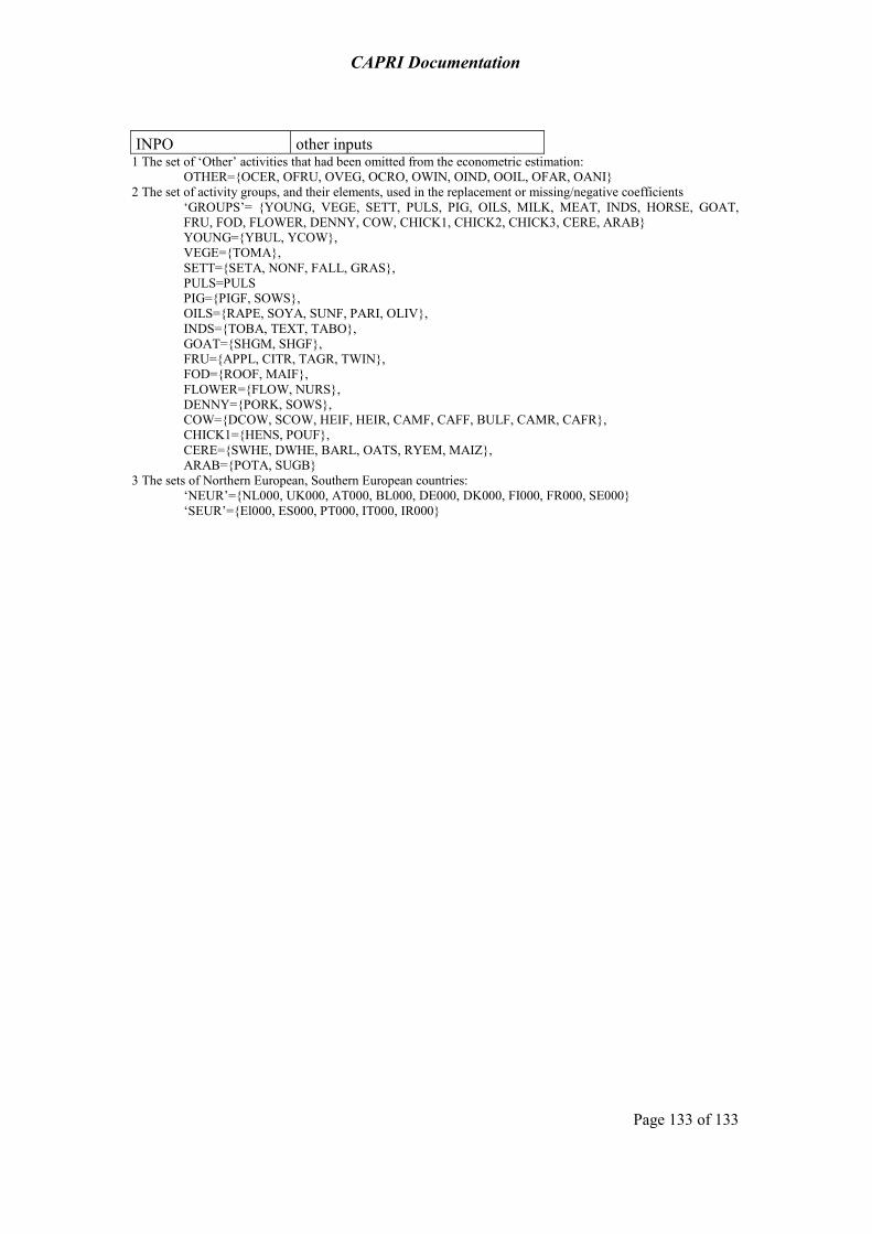
CAPRI Documentation

of 133

INPO other inputs 1 The set of ‘Other’ activities that had been omitted from the econometric estimation:

OTHER={OCER, OFRU, OVEG, OCRO, OWIN, OIND, OOIL, OFAR, OANI} 2 The set of activity groups, and their elements, used in the replacement or missing/negative coefficients

‘GROUPS’= {YOUNG, VEGE, SETT, PULS, PIG, OILS, MILK, MEAT, INDS, HORSE, GOAT, FRU, FOD, FLOWER, DENNY, COW, CHICK1, CHICK2, CHICK3, CERE, ARAB} YOUNG={YBUL, YCOW}, VEGE={TOMA}, SETT={SETA, NONF, FALL, GRAS}, PULS=PULS PIG={PIGF, SOWS}, OILS={RAPE, SOYA, SUNF, PARI, OLIV}, INDS={TOBA, TEXT, TABO}, GOAT={SHGM, SHGF}, FRU={APPL, CITR, TAGR, TWIN}, FOD={ROOF, MAIF}, FLOWER={FLOW, NURS}, DENNY={PORK, SOWS}, COW={DCOW, SCOW, HEIF, HEIR, CAMF, CAFF, BULF, CAMR, CAFR}, CHICK1={HENS, POUF}, CERE={SWHE, DWHE, BARL, OATS, RYEM, MAIZ}, ARAB={POTA, SUGB}

3 The sets of Northern European, Southern European countries: ‘NEUR’={NL000, UK000, AT000, BL000, DE000, DK000, FI000, FR000, SE000} ‘SEUR’={El000, ES000, PT000, IT000, IR000}

IPTS CAPRI Documentation - uni-bonn.de · PDF fileCAPRI Documentation Page 3 of 133...

Documents

Transcript of IPTS CAPRI Documentation - uni-bonn.de · PDF fileCAPRI Documentation Page 3 of 133...