Investor Sentiment and Commercial Real Estate Valuation

by

Jim Clayton*, David C. Ling**, and Andy Naranjo***

October 2007 Latest Revision: April 2008

Abstract

This paper investigates the role of fundamentals and investor sentiment in commercial real estate valuation. In real estate markets, heterogeneous properties trade in illiquid, highly segmented and informationally inefficient local markets. Moreover, the inability to short sell private real estate restricts the ability of sophisticated traders to enter the market and eliminate mispricing. These characteristics would seem to render private real estate markets highly susceptible to sentiment-induced mispricing. Using error correction models to carefully model potential lags in the adjustment process, this paper extends previous work on cap rate dynamics by examining the extent to which fundamentals and investor sentiment help to explain the time-series variation in national-level cap rates. We find evidence that investor sentiment impacts pricing, even after controlling for changes in expected rental growth, equity risk premiums, T-bond yields, and lagged adjustments from long run equilibrium. We thank the Real Estate Research Institute (RERI) for providing partial funding for this project. *Pension Real Estate Association, 100 Pearl Street, 13th Floor, Hartford, CT 06103, phone: (860) 692-6341, email: jim@prea.org; **Department of Finance, Insurance, and Real Estate, Hough Graduate School of Business, University of Florida, Gainesville, FL 32611-7168, phone: (352) 273-0313, email: ling@ufl.edu; ***Department of Finance, Insurance, and Real Estate, Hough Graduate School of Business, University of Florida, Gainesville, FL 32611-7168, phone: (352) 392-3781, email: andy.naranjo@cba.ufl.edu

1

Commercial Real Estate Valuation: Fundamentals versus Investor Sentiment

Introduction

Classical finance theory posits that prices of assets traded in relatively frictionless markets reflect

rationally estimated risk-adjusted discount rates and future income streams; there is no role for investor

sentiment. If mispricing does occur, it is quickly eliminated by the actions of informed arbitrageurs who

compete to capture the abnormal returns. The inability of the standard present value model to explain

dramatic run-ups and subsequent crashes in asset prices, such as the internet stock “bubble” in the late 1990s

and other price anomalies, has led to the development of the “behavioral” finance approach to asset

valuation. In these behavior models, investor sentiment can have a role in the determination of asset prices—

independent of market fundamentals.

The behavioral approach explicitly recognizes that some investors are not rational and that systematic

biases in these investor’s beliefs induce them to trade on non-fundamental information (i.e., sentiment).

Baker and Wurgler (2007) define investor sentiment as a misguided belief about the growth in future cash

flows or investment risks (or both) based on the current information set. The behavioral approach is also

predicated on “limits to arbitrage.” Arbitrageurs face non-trivial transaction and implementation costs that

prevent them from taking fully offsetting positions to correct mispricing. In addition, rational risk-averse

investors are unable to arbitrage away the mispricing because the unpredictability of investor sentiment

exposes them to “noise trader risk” (DeLong, Shleifer, Summers and Waldman, 1990). Hence, to the extent

that sentiment influences valuation, taking a position opposite to prevailing market sentiment can be both

expensive and risky. It is therefore important to understand the relative influence of fundamentals versus

sentiment in asset valuation.

Private commercial real estate markets are characterized by higher transaction costs and substantially

less liquidity than public stock markets. Thus, if relatively small frictions in the stock market can cause

sustained periods of overvaluation, it seems plausible to posit that private real estate markets are potentially

more susceptible to such episodes. The inability to short sell private real estate restricts the opportunity for

2

sophisticated traders to enter the market and eliminate mispricing, especially if they believe the property

market is overvalued. Limits to arbitrage might therefore be expected to lead to larger deviations of prices

from fundamental value in the presence of sentiment investors.

Despite the potential importance of investor sentiment in private real estate markets, no previous

research directly investigates the relative roles of fundamentals and investor sentiment in the pricing and

return generation process.1 This paper examines the relative influence of fundamentals and investor

sentiment in explaining the time-series variation in property-specific national-level capitalization rates.

Our specific innovations are twofold. First, we apply a new dataset to the study of cap rate determinants

that includes fundamental variables and survey (direct) measures of investor sentiment. We also use a

composite (indirect) measure of investor sentiment constructed from a set of sentiment proxies. Second, the

nature of our data allows us to utilize an innovative econometric approach to the analysis of the relation

between sentiment and property pricing. More specifically, we derive an equilibrium model of cap rates

specified as a function of real estate space and capital market fundamentals that is estimated using error-

correction techniques, thereby capturing both short and long-run pricing dynamics. The primary contribution

of the paper is the exploration of the impact of time-varying fundamentals and investor sentiment on property

pricing. To summarize our findings, we find evidence that investor sentiment significantly impacts pricing,

even after controlling for changes in expected rental growth, equity risk premiums, T-bond yields, and

lagged adjustments from long run equilibrium.

The remainder of the paper proceeds as follows. Section 2 discusses the relevant literature, including

key insights from sentiment-based theory of stock pricing as well as previous empirical studies of the

determinants of variations in real estate cap rates. In sections 3, 4, and 5 we present our conceptual and

empirical models of cap rates. Section 6 discusses the data. Sections 7 and 8 contain our empirical findings

and robustness checks. We conclude with a summary.

1 Hendershott and MacGregor (2005a, 2005b) test whether cap rates, and hence property values, reflect rational projections of future rental growth and expected returns, thereby providing an indirect test of the role of sentiment.

3

Background and Previous Literature

Both sentiment and limits to arbitrage are necessary conditions for the existence of mispricing. More

specifically, in a market characterized by heterogeneous investors, the existence of short sale constraints can

generate deviations in asset prices from fundamental values. Optimistic investors take long positions, while

pessimistic investors would like to take short positions. Short-sale constraints, however, may inhibit the

ability of rational investors to eliminate overpricing, even over sustained time periods. Therefore, rational

investors may sit on the sidelines when they believe prices are too high relative to fundamentals, leaving

market clearing prices to be determined, at the margin, by overly optimistic investors as in Baker and Stein

(2004).

Most behavioral finance research has followed a “bottom up” microeconomic approach that appeals to

biases in individual investor psychology to explain how and why investors might overreact or under-react to

past returns and information about market fundamentals.2 Brown and Cliff (2004, 2005) and Baker and

Wurgler (2006, 2007) offer a new “top down” macroeconomic approach, the first step of which is to derive

measures of aggregate investor sentiment for stocks. Brown and Cliff (2004, 2005) employ both survey

measures of investor sentiment as well as sentiment measures derived from a principal component analysis of

a set of potential sentiment proxies. They find that investor sentiment is highly correlated with

contemporaneous stock returns but has little short-run predictive power (Brown and Cliff, 2004). However,

taking a longer term perspective of two to three years, periods of high sentiment are followed by low returns

as the market mean reverts (Brown and Cliff, 2005).

Baker and Wurgler (2006, 2007) also employ principal component analysis to construct a sentiment

measure, and they extend the literature by quantifying the differential effect of sentiment on the cross-section

of stock returns by identifying which stocks are likely to be more affected by sentiment. Consistent with

model predictions, their results suggest that when beginning-of-period proxies for investor sentiment are high

2 Hirshleifer (2001) and Barberis and Thaler (2003) provide a review of the extensive behavioral finance literature.

4

(low), subsequent returns are relatively low (high) for stocks that are either more speculative in nature or for

which arbitrage tends to be particularly risky.

Real estate investors monitor market sentiment in several ways. First, they may subscribe to data

services that provide regular survey-based information about investment sentiment, such as the quarterly

RERC Real Estate Report used in this paper. Many investors also monitor variables related to “capital flows”

into the real estate sector. For example, they may track data on mortgage flows, the dollar volume and

number of properties sold, and capital flowing into real estate investment vehicles (e.g., commingled funds

for institutional and high net worth investors) under the belief that there is a common sentiment component

embedded in these investor activity variables.3

Although regarded as important by practitioners, there has been relatively little academic work aimed at

understanding the role of fundamentals versus investor sentiment and capital flows in real estate pricing

dynamics. A contemporaneous correlation between capital flows and cap rates does not by itself imply

causation. Capital flows and property prices (and hence cap rates) might both respond in a similar fashion to

fundamental economic variables and risk factors, such as unexpected inflation, changes in real interest rates,

or revisions in risk premiums. For example, if both capital flows and property prices increase when positive

economic news is released, a positive contemporaneous correlation between capital flows and cap rates does

not prove that capital flows cause or predict cap rates.

The lack of research examining the role of fundamentals versus sentiment and capital flows in real

estate markets is partly due to data limitations. Ling and Naranjo (2003, 2006) examine the dynamics of

commercial real estate capital flows and returns. Their work provides evidence that capital flows into public

(i.e., securitized) real estate markets do not predict subsequent returns, but that returns do affect subsequent

capital flows into these securitized real estate markets. Fisher, Ling, and Naranjo (2007) extend the work of

3 As part of the growing behavioral finance literature, researchers have also begun to carefully explore the impact of “flows” and trading activity on asset prices in public markets. See, for example, Warther (1995), Edelen and Warner (1999), Froot, O’Connell and Seasholes (2001), Brown, Goetzmann, Hiraki, Shiraishi, and Watanabe (2002), Griffin,

5

Ling and Naranjo (2003, 2006) by investigating the short- and long-run dynamics among institutional capital

flows and property returns in the largest U.S. metropolitan areas. The authors find some evidence that lagged

institutional capital flows influence current returns at the aggregate level, but the evidence is less convincing

when disaggregated by metropolitan area and property type. These papers provide useful empirical

characterizations of the dynamics of real estate capital flows and pricing, and therefore provide a solid

foundation on which additional research can build. However, their results do not directly address the role

sentiment plays in real estate markets, as they do not explicitly relate capital flows to investor sentiment

within a model of property pricing.

Shilling and Sing (2007) examine the rationality of investors’ expected income growth rates and total

return forecasts in private commercial real estate markets. Their findings are consistent with models of

investor irrationality. Furthermore, Shilling and Sing find evidence that investors act overly optimistic and

that they generally anchor their expectations to the previous period. Finally, Ling (2005) provides some

preliminary univariate evidence consistent with real estate pricing being driven at times by investor

sentiment.4

Modeling Prices and Cap Rates

Archer and Ling (1997) argue that three “markets” play a role in determining commercial real estate

prices: space markets, capital markets, and property markets. Local market rents are determined in the space

market (i.e., the market for leasable space). Required risk premiums for assets with varying profiles of cash

flow risk are determined in the capital market. Finally, property markets are where asset-specific discount

rates, property values, and cap rates are determined.

Property-specific discount rates are determined by the interaction of the risk-free rate, investor risk

premiums, and the risk profile of the specific property. For a given stream of expected net operating income

Nardari, and Stulz (2007), and Fama and French (2007). Clayton (2003) reviews much of this literature with a focus on the implications for private real estate.

(NOI), the equilibrium property price at time t, , should equal the present value of the NOIs discounted at

the assumed constant unlevered risk-adjusted rate, rt. That is,

etP

Tt

TTtT

t

t

t

t

t

et r

NSPgNOIr

gNOIr

gNOIr

NOIP)1(

)1(...

)1()1(

)1()1(

)1(1

333

2211

+++

++++

+++

++

= =−== , (1)

where T is the expected holding period in years and NSPT is the expected net sale proceeds in year T.5 It is

well known (e.g., Geltner, Miller, Clayton & Eicholtz, 2007, pages 209-210) that if, at time t, NOI is

expected to grow at a constant rate gt, and NSP is expected to remain a constant multiple of NOI, then

equation (1) simplifies to a valuation formula in which is solely a function of the expected growth in NOI

and the property specific risk-adjusted discount rate. That is,

etP

tt

et

ettt

et grNOI

Por

RNOI

grNOIP

−==

−=

1

1

11 (2)

Note that property values can be expressed as a multiple of first-year NOI, and the size of the multiple is

a function of (1) the property-specific discount rate and (2) expected changes in NOI.6 The equilibrium cap

rate at time t, , is merely the reciprocal of the value multiple. From equation (2), it follows that: etR

ttet grR −= . (3)

It is important to note that the level of NOI has no impact on the cap rate. Rather, it is the excepted change in

NOI that affects the price investors are willing to pay per dollar of first year NOI. Of course, it is unlikely

that NOI growth rates and future discount rates are expected to be constant forever. Nevertheless, equation

(3) is an approximation that motivates our empirical cap rate specification and is consistent with a more

4 Gompers and Lerner (2000) study the relationship between flow of funds (commitments) into venture capital funds and the valuation of new investments (firms) financed by the venture capital funds. Their findings are consistent with an uninformed demand /sentiment explanation of the link between fund flows and valuations. 5 NOI is assumed to include a reserve for expected capital expenditures and other nonrecurring expenses, such as leasing commissions.

6

6 State and federal income tax effects also affect property values and, therefore, price/NOI multiples, as may the amount and cost of mortgage financing.

7

general present value model that allows for time-variation in NOI growth and the discount rate to impact

commercial property valuation and hence the cap rate.7

The risk-adjusted discount rate has two components: RFt, the rate of return available on a risk-free U.S.

Treasury bond with a maturity equal to the expected holding period of the property; and RPt, the required

risk premium, which is property, market, and time dependent. Clearly, RFt, is determined outside local space

and property markets, as yields on Treasury securities are determined by the bid and ask prices of Treasury

market investors from around the world.

What about the determinants of RPt? In the capital markets, commercial real estate competes with all

other assets for a place in investors’ portfolios. According to classical portfolio theory, investors will select a

mix of investments based on the variances and covariances of the returns among the possible assets. As

investors bid for their optimal portfolio mix, their bidding simultaneously determines the required risk

premiums for the universe of investments according to their risk (variance and covariance) profiles. Thus,

the pricing of risk depends on risk preferences articulated in the broader capital as well as the specific risk

profile of the investment, which is determined by current and expected future conditions in the space market

in which the property is located.

The Dynamic Nature of Real Estate Pricing and Cap Rates

In highly liquid public securities markets, asset prices are believed to adjust quickly to changes in

market fundamentals such as interest rates, inflation expectations, and national and local market conditions.

However, in private, commercial real estate markets, observed cap rates may adjust more gradually to the

arrival of new information because of numerous property market inefficiencies, such as high transaction

7 Geltner and Mei (1995) and Plazzi, Torous and Valkanov (2004) both adapt variants of Campbell and Shiller’s (1998) log-linearized present value model with time-varying discount and “dividend” growth rates to study the relative contributions of time-variation in expected future returns versus property income in property valuation. Both studies

costs, lengthy decision making processes and due-diligence periods, and informational inefficiencies. A

number of authors have estimated structural models derived from theoretical cap rate models to investigate

property price dynamics (Sivitanides, Torto and Wheaton, 2001, Hendershott and MacGregor, 2005a, 2005b,

Chen, Hudson-Wilson and Nordby, 2004, Plazzi, Torous and Valkanov, 2004, Chichernea et al., 2007, and

Sivitanidou and Sivitanides, 1999).

To capture both long-run and short-run cap rate dynamics, we employ an error correction model (ECM)

similar to Hendershott and MacGregor (2005a). This framework allows us to model cap rates as an

adjustment process around equilibrium values. Error correction models are based on the idea that two or

more time series exhibit a long-run time-varying equilibrium to which the system tends to converge. The

long-run influence in the error correction model is achieved through negative feedback and error correction,

and this influence measures the degree to which long-run equilibrium forces drive short-run price dynamics

(see, for example, Engle and Granger, 1987, and Hamilton, 1994).

Following the Engle-Granger two-step method, a long-run cap rate model is specified in levels. The

second-stage, short-run, adjustment model is specified in first differences and includes a long-run error

correction term from the estimation of the long-run, equilibrium model. In the first-stage, theory and

econometric evidence are used to determine if the various data series contain unit roots and are cointegrated.

If the data series are cointegrated, a long-run equilibrium relation (i.e., a cointegrating regression) can be

specified in levels as:

,1

0 iit

n

iit XR υββ +∑+=

= (4)

where is the observed cap rate, and Xit are theoretically-based explanatory variables at time t. From this

regression, we can estimate residuals as the difference between the actual and estimated equilibrium values

tR

8

conclude that in the short run, property price fluctuations are driven primarily by changes in expected returns and not expected rents.

of the cap rate. 8 If the residuals from equation (4) are stationary, they may be used as an error correction

term in the short-run cap rate change model as follows:

,11

0 ttit

n

iit XR ευγαα +−Δ+=Δ −

∧

=∑ (5)

where is the first difference of the cap rate, ∆Xit are first differences of the explanatory

variables, and

1−−=Δ ttt RRR

1ˆ −tυ is the error correction term (the lagged residuals from the long-run regression).

Estimation of equation (5) provides evidence on short-run cap rate dynamics (the αi’s) and adjustments to the

previous disequilibrium in the long-run relation, γ (the speed of adjustment parameter). If γ=1, there is full

adjustment, while γ=0 suggests no adjustment. A more general specification of the short-run model may also

include multiple lags of the explanatory and dependent variables.

Empirical Specification

Based on our earlier theoretical discussion of equilibrium factors influencing cap rates, we employ the

following empirical model to each of the nine property types (see property type discussion in the next

section). In the first-stage, we estimate:

,3210 ttttt RFRPNOIGRWR υββββ ++++= (6)

where NOIGRWt is the expected growth in NOI, RPt is the unlevered equity risk premium, and RFt is the

yield-to-maturity on a 10-year Treasury security. In the second-stage, we estimate the following short-run

error correction model for each of the nine property types:

.13210 −

∧

+Δ+Δ+Δ+=Δ ttttt RFRPNOIGRWR υγαααα (7)

Equation (6) postulates that equilibrium cap rate levels are driven by two sets of influences: (1) discount

rate influences that reflect the risk-free opportunity cost of equity capital and the equity risk premium and (2)

9

8 The specification in equation (4) uses the results of equation (3) to specify the equilibrium cap rate as a function of the discount rate, rt, and expected NOI growth, gt, but does not impose the exact relationship, Rt = rt - gt , that holds under the constant growth assumption.

10

factors that influence the NOI growth expectations of investors (Wheaton et al., 2001). Cap rate changes

[equation (7)] are a function of changes in NOI, risk premiums, risk-free interest rates, and the degree to

which cap rates deviated from their equilibrium level in the previous time period.

Equation (6) reserves no explicit role for investor sentiment in the determination of observed cap rates.

To address this potential effect, we augment the specification in equation (7) with several measures of

investor sentiment. We also estimate variants of the second stage regression as additional robustness checks,

including specifications that allow us to test whether sentiment is embedded in market participants’ forecasts

of income growth and expected returns.

Data

Our primary data source is the Real Estate Research Corporation (RERC). Founded in 1931 in Chicago,

RERC is nationally known for its research, analysis, and investment criteria. Published quarterly in the Real

Estate Report, the RERC Real Estate Investment Survey summarizes information on current investment

criteria such as going-in (acquisition) cap rates, terminal cap rates, unlevered required rates of return on

equity, expected rental growth rates, and investment conditions provided by a sample of institutional

investors and managers throughout the U.S.9 According to RERC, the survey results are used by investors,

developers, appraisers, and financial institutions to “monitor changing market conditions and to forecast

financial performance.”10 As a robustness check, we also employ survey data from Korpacz

PriceWaterhouse Coopers.

Ideally, our cap rate data would be based on a large number of constant-quality (including location)

properties with identical lease terms. Such data do not exist. The RERC data, however, represent the cap

9 Several stock market studies find institutions to be informed investors; i.e., “smart money.” See, for example, Chakravarty (2001), Jones and Lipson (2004), and Sias, Starks, and Titman (2004). However, this evidence is tempered by studies that suggest institutions do not outperform individual investors (e.g., Nofsinger and Sias, 1999, and Kaniel, Saar, and Titman, 2005). 10 Real Estate Report, Summer 2002.

rates respondents are currently observing in the market for notional investment grade properties of constant

quality. Thus, these data are well-suited to our task, except they are not based on actual transactions.

Recall from equation (3) that equilibrium going-in cap rates ( ) are a function of unlevered discount

rates (rt) and expected growth rates in net rental income (gt). However, rt and gt cannot be directly observed.

Thus, in prior cap rate studies, proxies for these variables, or their component parts, were estimated. One

attraction of the RERC data is that expected rental growth rates and required equity returns are two of the

survey questions. In addition, survey respondents are asked to rank the “investment conditions” of various

property types and markets. These ranking of investment conditions directly measure investor sentiment.

etR

We focus first on the going-in capitalization rates reported by RERC for nine property types: apartment,

hotel, industrial research & development, industrial warehouse, central business district (CBD) office,

suburban office, neighborhood retail, power shopping centers, and regional malls. Survey cap rates for the

nine property types are displayed in Figure 1. During the first half of the 1996:Q1-2007:Q2 sample period,

cap rates remained relatively stable. However, beginning in 2002, cap rates on all property types began to

decline. For example, apartment cap rates stood at 8.7 percent in 2002:Q1; by 2007:Q2 they had declined

300 basis points to 5.7 percent.

To address potential concerns about the survey-based nature of our cap rate data, we compare RERC

cap rates, by property type, to cap rates obtained from two other sources, the National Council of Real Estate

Investment Fiduciaries (NCREIF) and Real Capital Analytics (RCA). NCREIF cap rates represent averages

derived from valuations of institutional class properties held by firms that are contributing members to the

NCREIF Property Index (NPI). RCA cap rates are averages derived from a much larger, but more

heterogeneous, population, coming from the sales of all properties of $5 million or more. NCREIF cap rates

are appraisal-based, and hence potentially backward looking. RCA cap rates are transaction-based, but

potentially noisy because they are not constant quality. NCREIF data extend back to 1990, whereas RCA

data begin in 2001. Correlations between RERC and NCREIF cap rate levels over the 1996:1 to 2007:2

period, and RERC and RCA cap rates over the 2001:1 to 2007:2 period, exceed 90 percent for all 9 property

11

12

types. Moreover, regressions of RERC cap rates on NCREIF (RCA) cap rates yield highly significant slope

coefficients of 0.80 (0.90) and above and R2s of 85 percent (90%) and above. In fact, regressions of RERC

cap rates on both NCREIF and RCA cap rates together result in adjusted R2s above 95 percent in almost all

nine cases. The tight connection between RERC cap rates and these two alternative series indicates that our

survey based cap rates are tracking pricing dynamics in commercial real estate markets very well.

Table 1 contains summary statistics, by property type, for our key RERC regression variables. The top

panel contains means, standard deviations, minimums, maximums, and serial correlations of levels and

changes for capitalization rates, expected rental growth rates, required equity returns, and investment

conditions. Mean expected rent growth ranges from 2.3 percent (annually) for power centers to 2.9 percent

for apartments. The levels of expect rent growth display substantial positive serial correlation across

quarters. However, changes in expected rental growth rates display significant negative serial correlation,

with the exception of apartments and hotels.

These data, coupled with our prior discussion of the cap rate determinants, provide a foundation for the

analysis of the widely discussed decline in US cap rates that has occurred since 2002. Most real estate

practitioners largely attribute the unprecedented decline in cap rates over this recent period to the “wall of

capital” and related liquidity that has permeated many markets, although market observers do not discount

the role declining interest rate levels have also played. However, inspection of the RERC data suggests a

more traditional explanation. In panels A-C of Figure 2, we plot RERC cap rates for apartments, CBD office

buildings, and regional malls. Also plotted are the corresponding RERC expected rental growth rates.

Theory tells us these two series should be negatively correlated, and this negative correlation is observed

over the 1996:Q1 to 2007:Q2 sample period.11 Similar correlations are observed for the remaining six

property types. Thus, it appears that the large cap rate declines since 2002 have been driven, at least in part,

by increases in expected rental growth.

11 Note that, in theory, cap rate movements are driven by variations in expected net rental income (NOI). We assume that such expectations are highly correlated with expected changes in market rental rates.

13

Note also that the observed increases in RERC expected rent growth are not consistent with increased

capital flows and rising prices. In fact, once market values exceed all-in construction costs, rising prices

(lower cap rates) produce increased construction that, in the longer run, leads to lower real rents. Said

differently, if increase capital flows and liquidity since 2002 were pushing asset values above fundamental

values, rational market participants should have been reducing their rent growth expectations, all else equal.

With the exception of hotel properties, average unlevered discount rates vary little across property type,

ranging from 10.2 percent for apartment properties to 10.9 percent for industrial R&D and suburban office

properties. This inability of survey respondents to detect cross property variation in ex ante risk premiums is

somewhat surprising given the significant variation in ex post returns earned by the various property types

over different historical time horizons. Shilling (2003) and Geltner et al. (2007) report a similar finding in ex

ante required returns derived from real estate investor surveys and also report that survey-based IRRs are

“too sticky” and overstated, at least historically. In contrast to cap rates, IRRs are difficult to observe

empirically. This raises the possibility that the RERC required IRRs may be measured with error and not

capturing true variation in risk premiums over time and across properties. We recognize this and account for

it in our empirical methodology.

Because OLS regressions with nonstationary variables produce spurious regression results, we test for

the stationarity of our regression variables using augmented Dickey-Fuller, Phillips-Perron, and Weighted

Symmetric unit root tests.12 Each of the tests includes intercept terms, time trends, and lags of the dependent

variables. Although not reported, each of the tests show that cap rates, rental growth rates, risk premiums,

and T-bond yields are each non-stationary (i.e., contain a unit root), but stationary in first differences at the 5

percent significance level. However, Engle-Granger and Johansen-Juselius cointegration tests reveal that cap

12 The Weighted Symmetric test is often recommended over the Dickey-Fuller test because it is more likely to reject the unit root null hypothesis when it is in fact false. That is, the Weighted Symmetric test has higher power. We also obtain similar results using the Phillips-Perron test. The Phillips-Perron test is a variant of the Dickey-Fuller test that addresses the problem of additional serial correlation in the residuals.

14

rates, rental growth rates, risk premiums, and interest rates are cointegrated, containing one cointegrating

vector among the variables at the 5 percent level. This suggests that a long-run equilibrium cap rate relation

(i.e., a cointegrating regression) can be specified in levels.

Measuring Real Estate Investor Sentiment

RERC survey respondents are asked to rank the current investment conditions for each of the nine

property types on a scale of 1 to 10, with 1 indicating “poor” investment conditions and 10 indicating

“excellent” conditions for investing. The bottom panel in Table 1 contains summary statistics for our RERC

investor sentiment variable. Note that the consensus opinion of survey respondents over the sample period

was that apartment properties, with an average rank of 6.3, were considered to be the most desirable

investments, followed by industrial warehouse and neighborhood retail properties. In contrast, retail power

centers, with a mean ranking of 4.8, were deemed the least desirable of the nine property types over the study

period. Inspection of Table 1 also reveals that RERC’s investment condition rankings display a significant

amount of variation over the sample period. For example, the investment desirability of hotels ranged from a

low of 2.7 to a high of 7.8. RERC sentiment levels display positive serial correlation across quarters.

However, changes in sentiment display significant negative serial correlation.

In addition to our RERC sentiment variable, we construct a measure of aggregate real estate investor

sentiment based on observable market level variables. More specifically, following Brown et al. (2002),

Brown and Cliff (2004) and Baker and Wurgler (2006), we construct an index of investor sentiment towards

commercial real estate investment based on the common variation in a number of proxies for sentiment.

More specifically, we extract an overall market sentiment measure from the following five sentiment-related

proxies: (1) commercial mortgage flows as a percentage of GDP; (2) the percentage of properties sold from

the NCREIF Property Index (NPI); (3) the ratio of the transaction based (TBI) and “constant liquidity”

15

versions of the NPI value index; (4) the NPI total return over the past four quarters; and (5) the most recent

quarterly TBI total return. 13

Mortgage flows are widely viewed by industry participants as a barometer of market investment

sentiment, in part because of the association between past real estate cycles and “excessive” mortgage flows

in periods of underpricing of default risk.14 The percentage of properties sold from the NPI and the ratio of

the TBI and constant liquidity versions of the NPI index are related to transaction activity or market turnover

and can also be viewed as market liquidity proxies.15 Our final two sentiment proxies are current property

returns derived from appraisal-based and transaction-based indices used by institutional investors to track

investment performance. We are not claiming that each of these time series represents investor sentiment,

but rather that if sentiment exists it is likely to be reflected to some degree in each, and it therefore can be

extracted as the common component.

To ensure our real estate sentiment measure is not an index of common business cycle risk factors, we

first regress each of the five sentiment proxies on the three-month Treasury yield, a term structure variable

(ten-year less three-month Treasury yield), and a measure of economy-wide default risk (the Baa corporate

bond yield less the AAA bond yield). We then construct our real estate sentiment index as the first principal

13 The NCREIF property index is comprised of the same class of properties and investors as the RERC survey. The quarterly “constant liquidity” version of the NPI is developed in Fisher, Geltner and Pollakowski (2007). The authors recognize that private, relatively illiquid asset markets adjust through both changes in prices and liquidity; observed transaction prices are conditional on overall market liquidity at the time of sale (i.e., price and liquidity are jointly determined). A “constant liquidity value” of a property is the value assuming no change in the level of market transaction activity; all adjustment takes place through price. The difference between the constant liquidity and hedonic value index, based on observed transaction prices that implicitly reflect time variation in liquidity, provides a calibration of commercial property liquidity. The TBI, including its constant liquidity version, are available at the MIT Center for Real Estate website. 14 Dokko et al. (1999) provide an overview of alternative explanations for real estate cycles that includes the potential role of mortgage flows. Pavlov and Wachter (2006) suggest that the underpricing of the borrowers’ put option in non-recourse commercial mortgage loans is at the root of the link between mortgage flows and property values. Riddiough (2008) argues that the securitization boom of the past 5 years has been accompanied by mispricing mortgage default risk that once again resulted in excessive mortgage flows and a bubble in commercial property prices. 15 Baker and Stein (2004) develop a theoretical model in which aggregate liquidity acts as an indicator of the relative presence of sentiment-based traders in the market place and therefore the divergence of asset price from fundamental value. Abnormally high aggregate liquidity (high turnover and/or low bid-ask spreads) is evidence of overvaluation, and in fact forecasts a downturn in stock prices.

16

component of the five residual series using quarterly observations over the 1984 to 2007:Q2 period. We

label this variable CLN (Clayton, Ling, and Naranjo) sentiment and include it in augmented versions of our

cap rate error correction model. This additional sentiment factor allows us to examine the extent to which

broader measures of real estate sentiment influence capitalization rates. Figure 3 displays the CLN sentiment

index and, as a check of consistency with the RERC survey data, compares it to an index constructed as the

first principal component of the RERC sentiment variable for the nine property types (RERC Sentiment).

Overall, our two sentiment proxies display substantial co-movement; in fact, the correlation between them is

0.76 over the 1996:Q1 to 2007:Q2 period.

Results

Table 2 contains parameter estimates and p-values (in parentheses) for our long-run model (equation 6)

for each of the nine property types over the 1996:Q1 to 2007:Q2 period. Consistent with established cap rate

theory, we include rent growth expectations, the risk premium embedded in required discount rates, and the

yield to maturity on 10-year Treasury bonds as our explanatory variables.

The estimated coefficient on the contemporaneous equity risk premium and T-bond yield are positive

and highly significant for all nine property types. The estimated coefficient on the risk premium ranges from

0.613 to 0.866 and averages 0.755 across the nine property types. The corresponding coefficient estimate on

the T-bond yield ranges from 0.579 to 0.871. The coefficient on expected rent growth is negative and highly

significant in all but the apartment, hotel, and neighborhood retail specifications. The adjusted R2 for our

nine long-run levels model averages 0.974.

Figure 4, panels A-C, contain plots of the actual and predicted cap rate values from the long-run

equation for apartments, CBD office buildings, and regional malls, respectively. As can be seen, the

estimated equations capture the broad movements in property specific cap rates, although errors do occur,

suggesting the appropriateness of our error correction framework.

17

We next estimate our cap rate change model (equation 7). Quarterly changes in all variables in the

long-run model are included in the error correction specifications, as well as the error correction term.16

Table 3 reports parameter estimates and p-values. As expected, the estimated coefficient on the change in

expected rent growth is negative and significant (at the 5% level) in the CBD office, suburban office, and

regional mall equations. However, the coefficient on expected rent growth is not significant in the remaining

six property type regressions.

Given the theoretical importance of expected rent growth in cap rate determination, the lack of

consistent significance of the RERC rent growth variable in our second-stage regressions, and the concern

that our RERC rent variable may be “sentiment-laden,” we experimented with several alternative proxies for

income growth expectations. More specifically, we obtained historical time series of effective rents from

Torto-Wheaton Research for the four main property types: office, industrial, retail, and apartments.

Following Sivitanides et al. (2001), we split expectations of nominal rent growth into growth due to expected

economy-wide inflation and expected real rent growth. We experimented with alternative proxies for

expected economy-wide inflation, including simple extrapolations of past changes in the Consumer Price

Index. We also investigated alternative proxies for real rent growth, including simple extrapolations and

more rational mean-reverting expectations. In short, these alternative specifications did not improve the

explanatory power of our rent growth variable; moreover, their use consumed several more degrees of

freedom. Thus, we report only those results obtained using the RERC rent growth variable.

The remaining explanatory variables enter the short-run cap rate regressions with the expected sign and

are highly significant. For example, the coefficient on the change in equity risk premium ranges from 0.533

to 0.794, all with p-values of 0.000. The estimated coefficients on changes in the 10-year T-bond yield are

of similar magnitude and significance. Thus, RERC cap rates strongly respond to changes in both the equity

risk premium and T-bond yield, as theory suggests. These results are consistent with previous studies that

16 The lagged cap rate change was initially included to expand the dynamic adjustment process. However, it was dropped from the analysis because in no specification was its estimated coefficient statistically significant.

18

find that cap rate changes are primarily driven by changing discount rates (i.e., Treasury yields and risk

premiums) rather than changes in rent growth expectations (Geltner and Mei, 1995, and Plazzi, Torous and

Valkanov, 2004).

As previously discussed, several rationales warrant the application of an error correction model to cap

rates, including the lagged and smoothed nature of appraisal-based prices and cap rates. Thus, the difference

between actual and predicted cap rates could reflect the aggregate effect of these underlying forces working

to return the market to equilibrium (Hendershott and MacGregor, 2005a). Examination of Table 3 reveals

that the error correction term carries the expected negative sign and is highly significant in all nine property

type regressions.

Finally, the adjusted R2 averages 0.642 across the nine cap rate change specifications, with a range of

0.507 to 0.712. The actual and fitted value for our apartment, CBD office, and regional mall data are

displayed in Panels A-C of Figure 5. Clearly, the error correction model picks up broad movements in cap

rates.

Sentiment Effects

As previously discussed, we employ two proxies for investor sentiment. The first is the RERC

“investment conditions” variable; the second is our constructed CLN sentiment index. Table 4 contains cap

rate change parameter estimates and p-values with the specification altered to include the change in RERC

sentiment from time t-1 to t. Although negative and statistically significant in the hotel regression (p-value

=0.064) and marginally significant in the industrial R&D and neighborhood retail equations, RERC

sentiment is not significant in the remaining six property type regressions. When the change in CLN

sentiment is substituted for the change RERC sentiment, the estimated coefficient is positive and significant

in the industrial warehouse and neighborhood retail equations only (see Panel B at the bottom of Table 4).

We also experimented with contemporaneous and lagged values of RERC and CLN sentiment, as well as

19

one, two, three, and four-quarter changes in both variables. Although several of these sentiment variables are

statistically significant in one or two of the nine cap rate regressions, the lack of a consistent sentiment effect

is noteworthy. These inconsistent sentiment effects are also robust over non-overlapping subsample

estimates (1996-2001 and 2002-2007).

A potential concern is that some of the explanatory variables in our reduced form error-correction model

are endogenous. For example, if a survey respondent is irrationally optimistic about the investment potential

of a particular property type, this non fundamentals-based optimism may bias downward the respondent’s

required risk premium and/or bias upward his or her expectations of future rental growth. Said differently,

our RERC required risk premiums and/or rental growth expectations may be sentiment laden. This, in turn,

may reduce the explanatory power of our sentiment proxies in the cap rate change regressions.

To address this issue, we orthogonalize our expected rent growth and risk premium variables with

respect to our sentiment variables. This orthogonalization is designed to strip these fundamental variables of

sentiment and load the explanatory power of investor sentiment onto the estimated RERC and CLN

coefficients in our cap rate change regressions. The results with the orthogonalized expected rent growth and

risk premium variables and RERC sentiment are reported in Panel A of Table 5. First, note that the adjusted

R2s are unchanged from Table 4. This is because the information on the right-hand-side of the cap rate

change models is not altered by the orthogonalization of rent growth and risk premiums with respect to

sentiment. However, the estimated coefficient on the change in RERC sentiment is negative and highly

significant in all but the regional mall equation. Thus, although fundamentals are the primary determinants

of cap rates, sentiment also has an impact on cap rate determination.

It is also important to note that the estimated coefficients on our fundamental variables are little changed

by the orthogonalization (compare Panel A in Tables 4 and 5). This suggests that, although

orthogonalization of the rent growth and risk premium variables is necessary to isolate the effect of sentiment

on cap rates, this orthogonalization does not alter our conclusions about the effects of fundamental variables

on cap rates.

20

We also orthogonalized rent growth and the risk premium with respect to CLN sentiment and estimated

our cap rate change regressions using CLN as our proxy for investor sentiment. The estimated coefficients

on CLN sentiment, reported in Panel B of Table 5, are negative and highly significant in all nine property

type regressions. Thus, our finding of a role for sentiment in cap rate determination is not dependent on our

choice of sentiment proxy.

Robustness Results Using Alternative Database

Finally, to further examine the robustness of our results, we repeat our estimations using survey data

from Korpacz Pricewaterhouse Coopers (KPC). Similar to the RERC survey, the KPC survey consists of

quarterly responses from 100-odd prominent pension plans, foundations, endowments, life insurance

companies, investment banks, and REITs that invest in U.S. real estate. The KPC survey has been conducted

each quarter since 1988 and contains rich information on the expectations of participants in commercial real

estate markets. Survey respondents are asked to report the cap rates they are observing on CBD office

buildings, major retail properties, apartment buildings, and industrial warehouses. The survey also asks

respondents for their required (unlevered) rates of return and rental growth forecasts for each of these

property types. Thus, the KPC survey provides us with cap rates and their fundamental determinants:

expected rental growth and required rates of return. However, all retail and industrial property types are

aggregated together in the KPC survey. Thus, the results are not directly comparable to our retail and

industrial RERC results, which are disaggregated by subproperty type. However, the KPC data for

apartments and CBD office properties are directly comparable to our RERC data.

The error correction model results using the KPC data for apartments and CBD office properties are

very similar to the corresponding results from the RERC estimations over the 1996:2 to 2007:2 sample

period. For example, using RERC data, we report in Table 4 that the estimated coefficients on Risk Premium

Change and Treasury Yield Change in the short-run CBD model (without orthoganalization) are 0.535 and

0.599, respectively, and both are highly significant. The corresponding coefficient estimates using KPC data

are 0.581 and 0.476, and both estimates are, again, highly significant. The coefficient on the error correction

21

term using the RERC data and KPC date are, -0.708 and -0.439, respectively. The only substantive

difference in the results is that the estimated coefficient on Rent Growth Change is negative and significant

in the RERC estimation. Although negative, this coefficient estimate is not significant in the KPC estimation.

Our error correction model results for apartments using KPC data are also very similar to the RERC

results. In particular, the estimated coefficients on Risk Premium Change and Treasury Yield Change in the

short-run CBD model are positive and highly significant, although the magnitude of the estimates is less than

in the RERC estimations. The estimated coefficient on the error correction term is negative and significant,

but it is also smaller in magnitude than the estimate obtained with RERC data.

Overall, the error correction results using KPC data for apartments and CBD office properties indicates

that our primary findings are robust to the use of an alternative dataset.

A Vector Error-Correction Model

To further examine potential endogeneity effects, we also estimate a vector error-correction model

(VECM) in which all of the variables are specified as endogenous variables in a five equation system. A

VECM model is a restricted vector autoregressive (VAR) model designed for use with nonstationary time

series that are cointegrated (see, for example, Hamilton, 1994). A group of nonstationary time-series is

cointegrated if there is a linear combination of them that is stationary. These cointegrating relations (error

correction terms) are incorporated into the VECM.17

For example, consider the following two-variable VECM:

ΔYt = a1 + b1ΔYt-1 + c1ΔZt-1 + α1(Yt-1 - βZt-1) + e1t (8)

ΔZt = a2 + b2ΔZt-1 + c2ΔYt-1 + α2(Yt-1 - βZt-1) + e2t, (9)

where all terms involving Δ are stationary. This two-variable error correction model is a bivariate VAR in

first differences augmented by the error-correction terms α1(Yt-1 - βZt-1) and α2(Yt-1 - βZt-1) from the

17 An alternative approach would be to estimate a structural equation system. However, this would require identifying restriction assumptions and would also be problematic given the non-stationary and cointegrated nature of our data.

cointegrating relation. The β’s contain the cointegrating equation and the α‘s the speeds of adjustment. In

general, the kth order vector error-correction model can be represented by the following system:

,... 112211 tktktkttt eXXXXX +Π+ΔΓ++ΔΓ+ΔΓ+=Δ −+−−−−μ (10)

where

Xt = vector of p I(1) variables,

μ = p x 1 vector of intercepts,

Γ1, Γ2, Γk, Π = p x p matrices of parameters,

et = error term [∼ NID(0,Ω)],

Δ = difference operator, and

I(1) = integrated of order one (i.e., first-difference stationary).

In the above system, the coefficient matrix Π provides information about the long-run equilibrium (error

correction) relations among the variables, while the Γ’s provide information on short-run relations. If all of

the elements of Π equal zero, the system becomes a traditional VAR in differences. Using Johansen’s (1988)

method, we first obtain the number of cointegrating vectors (rank of Π) and then the parameter estimates

using the VECM.

As discussed earlier, augmented Dickey-Fuller and Weighted Symmetric unit root tests suggest that the

variables in the system are non-stationary (i.e., we could not reject the null hypothesis of a unit root at the 5

percent significance level for the variables in the system). The results of Johansen’s (trace) cointegration

tests also indicate the existence of one cointegrating vector at the 5 percent level.

22

Table 6 reports the VECM estimation results for the cap rate equation using our RERC sentiment

variable. Similar to our earlier single-equation error correction model results, we find that cap rate changes

are positively related to changing Treasury yields and equity risk premiums, although the statistical

significance of these two fundamental variables is reduced relative to their significance in our single equation

error correction model. However, we find no consistent role for sentiment in explaining the time series

variation of cap rates during the 1996:Q1 to 2007:Q2 sample period. Finally, in contrast to our earlier results,

23

we find that the error correction term (cointegrating equation) is often insignificant in the VECM results.

This finding is consistent with McGough and Tsolacos (2001) and may result from a limited degrees of

freedom problem whereby numerous parameters are being estimated in the system of equations with a

limited number of quarterly observations.

The estimation results for the RERC sentiment equation in the VECM also allows us to formally test

whether RERC sentiment is explained by lagged changes in our two fundamental variables: equity risk

premiums and expected rental growth rates. The results (not shown) indicate that changes in RERC

sentiment are not driven by these two fundamental variables. In fact, the only variable that consistently

explains the change in RERC sentiment in the current quarter is the prior quarter’s change, although this may

again reflect the inability of our sample size to fully support the estimation of the VECM.

As noted above, our inability to uncover a role for sentiment in explaining the time-series variation in

cap rates over the 1996:Q1 to 2007:Q2 sample period may be the result of limited degrees of freedom in our

VECM estimation using RERC data. However, the KPC data for apartments and CBD office properties

extends back to 1991:Q4, providing more degrees of freedom than the RERC data. To examine the

robustness of our VECM results to the use of a longer time series, we replicated the RERC VECM results

reported in Table 6 using the KPC data. The results are encouraging. The estimated coefficient on Risk

Premium Chg(-1) for apartments reported in Table 6 is 0.375 (t-statistic=1.906). The corresponding estimate

using the KPC data is 0.243 (t-statistic=2.625). Similarly, the coefficient on Treasury Yield Chg(-1) using

RERC data is 0.340 (t-statistic= 1.690). The corresponding estimate using the KPC data is 0.239 (t-

statistic=2.474). Overall, the significance of the fundamental variables increases somewhat using a longer

time series. Interestingly, unlike the RERC VECM estimations, the coefficient on Sentiment Chg(-1) is

negative and significant and the coefficient on Sentiment Chg(-2) is positive and significant, suggesting a

role for sentiment in the determination of apartment cap rates.

The use of the KPC data with a longer time series in the estimation of the CBD office VECM provides

similar results. That is, coefficients on the fundamental variables carry the expected sign and significance

24

,

t,

(with the exception of expected rent growth). In addition, however, the estimated coefficient on RERC

sentiment Chg(-1) is -0.257 (t-statistic=-2.220). In summary, the use of the VECM, which allows all

variables in the system to be estimated endogenously, also suggests a statistically significant role for

sentiment when the longer KPC time series is used.

Time Variation in the Dispersion of Cap Rates, Rent Growth, and Discount Rates

Our earlier single-equation error correction results suggest that sentiment plays a role in commercial

property cap rate determination, once we account for the sentiment embedded in the expected rent growth

and risk premiums. In addition to endogeneity issues, another potential concern is that our testing approach

implicitly assumes that if sentiment impacts prices it does so at all times. That is, sentiment is essentially

another variable in the property pricing equation. However, sentiment may only play a pricing role in “up”

or “hot” markets. 18 Short-sale constraints inhibit the ability of rational investors to eliminate overpricing

and may imply that irrational investors are only active in the market when they are overly optimistic. Hence

in up markets, asset values reflect the sentiment of these irrational traders. Our tests of a role for sentimen

therefore, may have relatively low power because sentiment is not important in all periods in the sample.

To address this concern, we provide an additional test for the role of sentiment in property pricing

dynamics. More specifically, we examine the time series of the coefficient of variation of RERC cap rates,

rent growth, discount rates and sentiment, calculated across the nine property types each quarter and test

whether variation over time in these cross-sectional dispersion series is related to investor sentiment, after

controlling for macroeconomic fundamentals. If sentiment does impact pricing, we expect that in periods of

high sentiment there will be less cross-sectional dispersion in cap rates and discount rates because all assets

in a given “bucket” experience the upswing. That is, cross-property dispersion in pricing will decrease as

comovement in returns tightens and is delinked from comovement in cash flow and risk fundamentals due to

18 See, for example, Baker and Stein (2004). Yu and Yuan (2007) also find that irrationality is more prevalent in rising markets.

25

coordinated sentiment-based trading (Barberis, Shleifer and Wurgler, 2002). In contrast, cross-sectional

variation is likely to increase during economic downturns (Plazzi et al. 2008).

Figure 6 presents the time series of cross-property standard deviations (top graph) and coefficients of

variation (bottom graph) of the RERC regression variables. Note that, starting in 2000, the dispersion of

RERC sentiment across the nine property types declines, with the dispersion of cap rates and discount rates

following soon thereafter. Interestingly, there does not appear to be any systematic change in the variation of

rent growth expectations over this time period, except for the much higher coefficient of variation during the

recession of 2002, suggesting that the decrease in discount rate and cap rate dispersion is either a sentiment

or a capital market (i.e., denominator) phenomenon.

To investigate whether the lower volatility resulting from convergence across property types represent

rational repricing based on economic fundamentals or, instead, derives from investor sentiment, we regress

the time series of cross property standard deviations on our CLN sentiment measure and three economic

factors that have been found to be related to business cycle risks in previous studies; the three-month

Treasury yield, the Treasury term structure, and a corporate default premium variable.19 All explanatory

variables are lagged to avoid simultaneity bias, and lagged dependent variables are included as regressors to

account for slow adjustment over time. Table 7 reports the estimation results. Cross-property dispersion in

cap rates is strongly persistent, and the coefficients on both the three-month Treasury yield and CLN

sentiment are statistically significant and negative. Hence, high investor sentiment predicts a decrease in the

cross-property dispersion of cap rates, consistent with our hypothesis about a convergence in pricing during a

hot market. We obtain similar results with the IRR dispersion equation, although the statistical significance

is not quite as high as in the cap rate equation. Finally, sentiment does not appear to affect the variation in

rental growth rates. Overall, these findings suggest that the decrease in cap rates and required returns over the

past five-to-six years is a capital market phenomenon that may, in part, reflect investor sentiment.

19 The version of the CLN sentiment index used here is the principal component of the sentiment proxies after first orthogonalizing each proxy by regressing it on the three economic fundamental variables.

26

Conclusion

Classical finance theory posits no role for investor sentiment, capital flows, or trading activity. Rather,

assets are assumed to trade in frictionless markets where unemotional investors force prices to equal the

rational present value of expected future cash flows. However, the inability of the standard present value

model to explain several dramatic run-ups and subsequent crashes in asset prices has led to a burgeoning

“behavioral” finance literature. This behavioral paradigm allows for the existence of both irrational investors

and limits to arbitrage. In these models, investor sentiment, capital flows, and trading volume can have a

role in the determination of asset prices—independent of market fundamentals.

Private commercial real estate markets differ substantially from public stock markets. First, real estate

assets are decidedly heterogeneous. Therefore, unlike the listed shares of a firm for which close substitutes

exist either directly of indirectly, the unique location and other attributes of commercial real estate assets

severely restrict an investor’s set of acceptable substitutes. Moreover, these heterogeneous assets trade in

illiquid, highly segmented and informationally inefficient local markets. As a result, the search costs

associated with matching buyers and sellers are significant. The inability to short sell private real estate also

restricts the ability of sophisticated traders to enter the market and eliminate mispricing, especially if they

believe property is overvalued. Limits to arbitrage could therefore be expected to lead to large deviations of

prices from fundamental value in the presence of sentiment investors.

These characteristics of private real estate markets would seem to render them highly susceptible to

sentiment-induced mispricing and, indeed, there is a widespread belief among many real estate market

participants that real estate markets are subject to fads (i.e., swings in sentiment). Many real estate

practitioners devote considerable effort to understanding market sentiment (i.e., what other investors might

do), rather than focusing solely on cash flow and discount rate considerations. In fact, the significant

reduction in capitalization rates that occurred in most commercial real estate markets from 2002 to 2007 is

largely, if not entirely, attributed to the surge in sentiment-driven capital flows that occurred during this

period (Downs, 2004, House, 2004).

27

Despite the potential importance of fundamentals and investor sentiment in private real estate pricing

dynamics, no research exists that directly examines the relative influence of fundamentals and investor

sentiment in commercial real estate pricing. This paper examines the extent to which fundamentals and

investor sentiment explain the time-series variation in property-specific national cap rates.

In our analysis, we apply a new dataset to the study of cap rate determinants that includes fundamental

variables and survey (direct) measures of investor sentiment. We also use a composite (indirect) measure of

investor sentiment constructed from a set of sentiment proxies. Direct survey measures of investor

sentiment, along with cap rates, unlevered equity discount rates, and expected rent growth for nine property

types at both the national and MSA-level are taken from the Real Estate Report, published quarterly by the

Real Estate Research Corporation (RERC). The nature of the RERC data set also allows us to utilize an

innovative modeling and econometric approach to the analysis of the relation between sentiment and

property pricing. More specifically, we derive an equilibrium model of cap rates specified as a function of

real estate space and capital market fundamentals that is estimated using error-correction techniques, thereby

capturing both short and long-run dynamics.

Our results show that fundamentals are the key driver of cap rates. However, sentiment also plays a

pricing role over our 1996-2007 study period.

References Archer, W.A. & D.C. Ling (1997) “The Three Dimensions of Real estate Markets: Linking Space, Capital, and Property Markets,” Real Estate Finance, Fall, 7-14. Baker, M. & J. Stein (2004) “Market liquidity as a sentiment indicator,” Journal of Financial Markets, 7, 271-299. Baker, M. & J. Wurgler (2006) “Investor Sentiment and the Cross-Section of Stock Returns,” Journal of Finance, 61(4): 1645-1680. Baker, M. & J. Wurgler (2007) “Investor Sentiment in the Stock Market,” The Journal of Economic Perspectives, 21, 129-151. Barberis, N. and R. Thaler (2003) “A Survey of Behavioral Finance,” Chapter 18 in Handbook of the Economics of Finance, Vol. 1, Part 2, pp. 1053-1128, Elsevier.

28

Barberis, N., A. Shleifer and J. Wurgler (2005) “Comovement,” Journal of Financial Economics 75: 283–317 Brown, G. & M. Cliff (2004) “Investor sentiment and the near term stock market,” Journal of Empirical Finance, 11, 1-27. Brown, G. & M. Cliff (2005) “Investor Sentiment and Asset Valuation,” Journal of Business, 78(2): 405-440.

Brown, S., W. Goetzmann, T. Hiraki, N. Shiraishi, & M. Watanabe (2002) “Investor Sentiment in Japanese and U.S. Daily Mutual Fund Flows,” Yale Working Paper.

Campbell, J. and R. Shiller (1998) “The Dividend-Price Ratio and Expectations of Future Dividends and Discount Factors,” Review of Financial Studies, 1. Chakravarty, S. (2001) “Stealth-Trading: Which Trader’s Trades Move Stock Prices?, Journal of Financial Economics, 61, 289-307. Chen, J., S. Hudson-Wilson & H. Nordby (2004) “Real Estate Pricing: Spreads and Sensibilities: Why Real Estate Pricing is Rational,” Journal of Real Estate Portfolio Management, 10, 1-21.

Chichernea, D., N. Miller, J. Fisher, M. Sklarz & R. White (2007) “A Cross Sectional Analysis of Cap Rates by MSA,” Working Paper (forthcoming Journal of Real Estate Research).

Clayton, J. (2003) “Capital Flows and Asset Values: A Review of the Literature and Exploratory Investigation in a Real Estate Context,” Homer Hoyt/University of Cincinnati Working Paper.

Clayton, J., G. MacKinnon & L. Peng (2007) “Time Variation of Liquidity in the Private Real Estate Market: An Empirical Investigation,” Journal of Real Estate Research (forthcoming).

De Long, J. Bradford, A. Shleifer, L.H. Summers, and R.J. Waldmann (1990) Noise trader risk in financial markets, Journal of Political Economy 98:4, 703-738.

Dokko, Y., R. Edelstein, A. Lacayo and D. Lee (1999) “Real Estate Income and Value Cycles: A Model of Market Dynamics,” Journal of Real Estate Research, 18(1).

Downs, Anthony, 2004, “Some Aspects of the Real Estate Outlook” (www.anthonydowns.com).

Edelen, R. M. & J. B. Warner (2001) “Aggregate Price Effects of Institutional Trading: A Study of Mutual Fund Flow Data and Market Returns,” Journal of Financial Economics 59(2): 195-220.

Engle, R. and C.W.J Granger, 1987, “Cointegration and Error Correction: Representation Estimation and Testing,” Econometrica 55: 251-276.

Fisher, J., D.C. Ling, & A. Naranjo (2007) “Commercial Real Estate Return Cycles: Do Capital Flows Matter?,” University of Florida/RERI Working 1aper.

Froot, K.A., P.G.J. O’Connell, & M.S Seasholes (2001) “The Portfolio Flows of International Investors,” Journal of Financial Economics 59(2): 151-194.

29

Geltner, D. and J. Mei (1995) “The Present Value Model with Time-Varying Discount Rates: Implications for Commercial Property Valuation and Investment Decisions, The Journal of Real Estate Finance and Economics, 11(2).

Geltner, Miller, Clayton & Eicholtz (2007), Commercial Real Estate Analysis and Investments (2nd edition), South-Western Publishing.

Gompers, P. & J. Lerner (2000) “Money Chasing Deals? The Impact of Fund Inflows on Private Equity Valuations,” Journal of Financial Economics, 5, 281-325.

Greene, W. (1993) Econometric Analysis (2nd Edition), Englewood Cliffs: Prentice Hall.

Griffin, J., F. Nardari & R. Stulz (2007) “Stock Market Trading and Market Conditions,” The Review of Financial Studies (forthcoming).

Hamilton, J.D., 1994, Time Series Analysis, Princeton: Princeton University Press.

Hendershott, P.H. & B. MacGregor (2005a) “Investor Rationality: Evidence from U.K. Property Capitalization Rates,” Real Estate Economics, 26, 299-322.

Hendershott, P.H. & B. MacGregor (2005b) “Investor Rationality: An Analysis of NCREIF Commercial Property Data,” Journal of Real Estate Research, Vol. 26.

Hirshleifer, D. (2001) “Investor Psychology and Asset Pricing,” Journal of Finance 56, 1533-1597.

House, Garret C., 2004, “Demand for Real Estate: Capital Flows, Motivations, and the Impact of Rising Rates,” Institute for Fiduciary Education. Jones, C.M. and M. Lipson (2004) “Are Retail Orders Different? Working Paper, Columbia University. Kaniel, R., G. Saar and S. Titman (2005) “Individual Investor Sentiment and Stock Returns.” Working Paper, Duke University. Ling, D.C. (2005) “A Random Walk Down Main Street: Can Experts Predict Returns on Commercial Real Estate?” Journal of Real Estate Research, Vol. 27, No. 2, pp. 137-154.

Ling, D.C. & A. Naranjo (2003) “The Dynamics of REIT Capital Flows and Returns,” Real Estate Economics 31.

Ling, D.C. & A. Naranjo (2006) “Dedicated REIT Mutual Fund Flows and REIT Performance,” Journal of Real Estate Finance and Economics, Vol. 32, No. 4, pp. 409-433.

McGough, T. and S. Tsolacos (2001) “Do Yields Reflect Property Market Fundamentals?, Working Paper, City University Business School. Nofsinger, J.R. and R.W. Sias (1999) “Herding and Feedback Trading by Institutional and individual investors,” Journal of Finance, 59, pgs. 2263-2295. Pavlov, Andrey D. and Wachter, Susan M. (2006) "Underpriced Lending and Real Estate Markets". Available at SSRN: http://ssrn.com/abstract=980298

30

Plazzi, A., Torous, W. N., and Valkanov, R. (2004) “Expected Returns and the Expected Growth in Rents of Commercial Property,” Working Paper, The Anderson School at UCLA.

Plazzi, A., Torous, W. N., and Valkanov, R. (2008) “The Cross-Sectional Dispersion of Commercial Real Estate Returns and Rent Growth: Time Variation and Economic Fluctuations”, forthcoming, Real Estate Economics, 2008.

Riddiough, T. (2008) “On the Addictive Properties of Cheap and Easy Debt Capital,” PREA Quarterly, Winter issue (forthcoming). Shilling. J.D. (2003) “Is There a Risk Premium Puzzle in Real Estate?” Real Estate Economics, Vol. 31, No. 4, pp. 501-525. Shilling, J.D. and T. F. Sing (2007) “Do Institutional Real Estate Investors have Rational Expectations?” Working Paper. Sias, R., L.T. Starks, and S. Titman (2004) “Changes in Institutional Ownership and Stock Returns: Assessment and Methodology,” Journal of Business, forthcoming. Sivitanidou, R. and P. Sivitanides (1999) “Office Capitalization Rates: Real Estate and Capital Market Influences,” Journal of Real Estate Finance and Economics, Vol. 18, No. 3, pp. 297-322.

Sivitanides, P., J. Southard, R. Torto and W. Wheaton (2001) “The Determinants of Appraisal-Based Capitalization Rates,” MIT Working Paper.

Warther, V.A. (1995) “Aggregate Mutual Fund Flows and Security Returns,” Journal of Financial Economics 39.

Wheaton, W. (1999) “Real Estate Cycles: Some Fundamentals,” Real Estate Economics 27. Yu, J. and Yu Yuan (2007) “Investor Sentiment and the Mean-Variance Relation,” Working Paper, Wharton School, University of Pennsylvania.

Figure 1 Cap Rate Levels by Property Type

5.0

6.0

7.0

8.0

9.0

10.0

11.0

12.0

1996Q1

1996Q3

1997Q1

1997Q3

1998Q1

1998Q3

1999Q1

1999Q3

2000Q1

2000Q3

2001Q1

2001Q3

2002Q1

2002Q3

2003Q1

2003Q3

2004Q1

2004Q3

2005Q1

2005Q3

2006Q1

2006Q3

2007Q1

Cap

 Rate (%

)

Cap Rate Levels

Apart

Hotel

Ind R&D

Ind Ware

CBD Office

Sub Office

Neigh Ret

Power Center

Malls

Cap rates are obtained from the Real Estate Research Corporation’s Real Estate Report, which publishes results from RERC’s quarterly Real Estate Investment Survey. The Real Estate Report summarizes the expected rates of return, property selection criteria, and investment outlook of a sample of institutional investors and managers throughout the U.S. The property level cap rates displayed in Figure 1 are aggregated across all metropolitan markets.

31

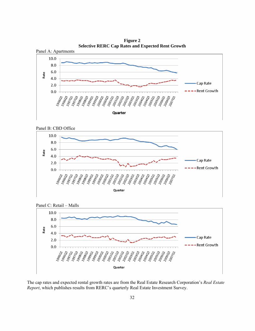
Figure 2 Selective RERC Cap Rates and Expected Rent Growth

Panel A: Apartments

Panel B: CBD Office

Panel C: Retail – Malls

The cap rates and expected rental growth rates are from the Real Estate Research Corporation’s Real Estate Report, which publishes results from RERC’s quarterly Real Estate Investment Survey.

32

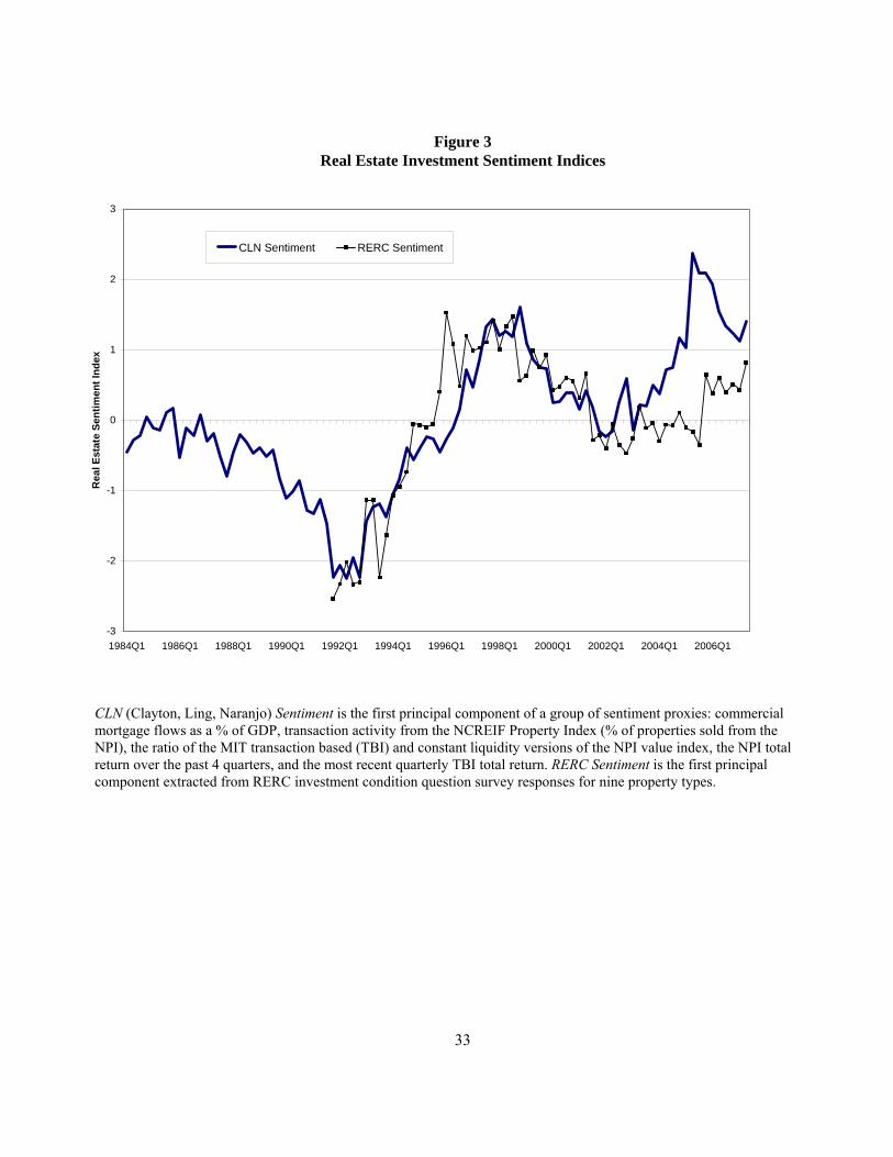
Figure 3 Real Estate Investment Sentiment Indices

-3

-2

-1

0

1

2

3

1984Q1 1986Q1 1988Q1 1990Q1 1992Q1 1994Q1 1996Q1 1998Q1 2000Q1 2002Q1 2004Q1 2006Q1

Rea

l Est

ate

Sent

imen

t Ind

ex

CLN Sentiment RERC Sentiment

CLN (Clayton, Ling, Naranjo) Sentiment is the first principal component of a group of sentiment proxies: commercial mortgage flows as a % of GDP, transaction activity from the NCREIF Property Index (% of properties sold from the NPI), the ratio of the MIT transaction based (TBI) and constant liquidity versions of the NPI value index, the NPI total return over the past 4 quarters, and the most recent quarterly TBI total return. RERC Sentiment is the first principal component extracted from RERC investment condition question survey responses for nine property types.

33

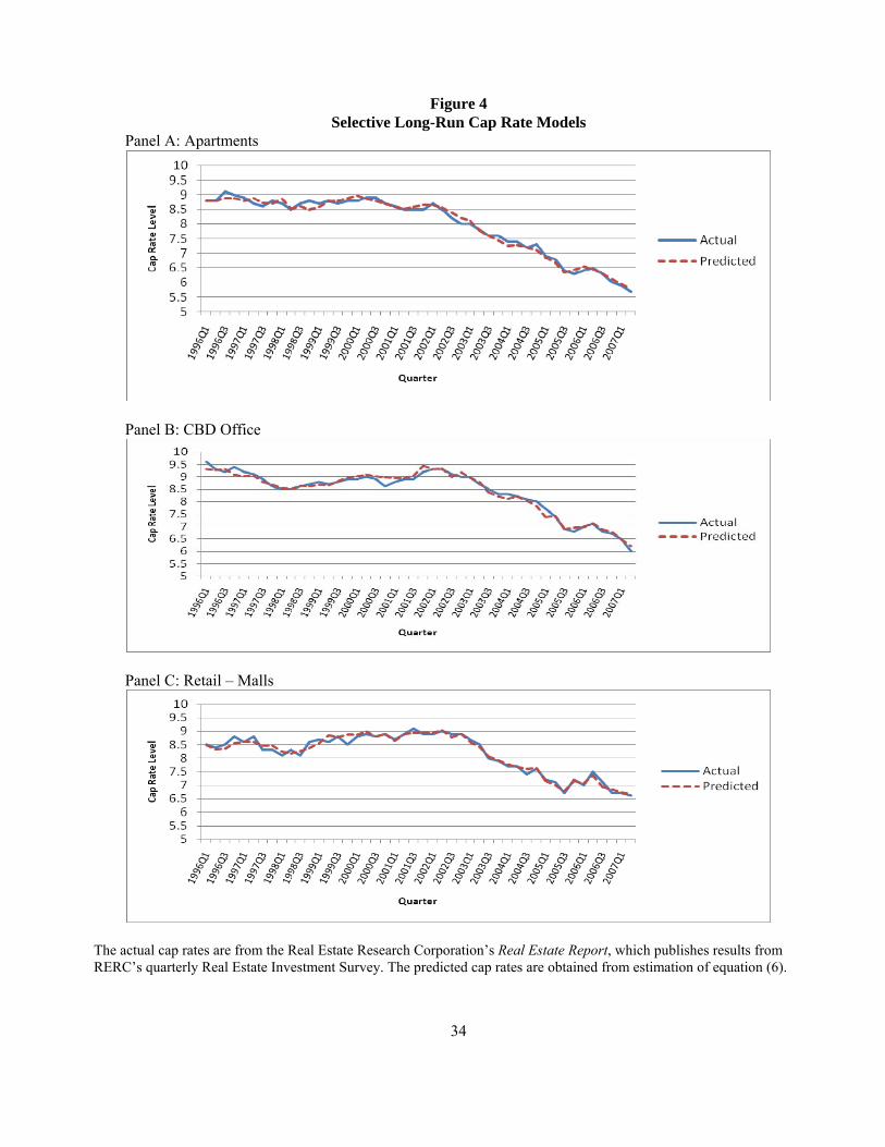
34

Selective Long-Run Cap Rate Models Panel A: Apartments

Figure 4

Panel B: CBD Office

Panel C: Retail – Malls

The actual cap rates are from the Real Estate Research Corporation’s Real Estate Report, which publishes results from RERC’s quarterly Real Estate Investment Survey. The predicted cap rates are obtained from estimation of equation (6).

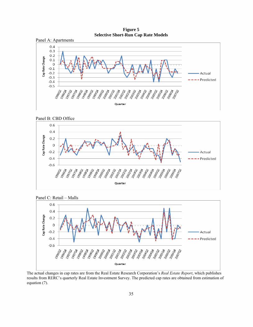
Figure 5 Selective Short-Run Cap Rate Models

Panel A: Apartments

Panel B: CBD Office

Panel C: Retail – Malls

The actual changes in cap rates are from the Real Estate Research Corporation’s Real Estate Report, which publishes results from RERC’s quarterly Real Estate Investment Survey. The predicted cap rates are obtained from estimation of equation (7).

35

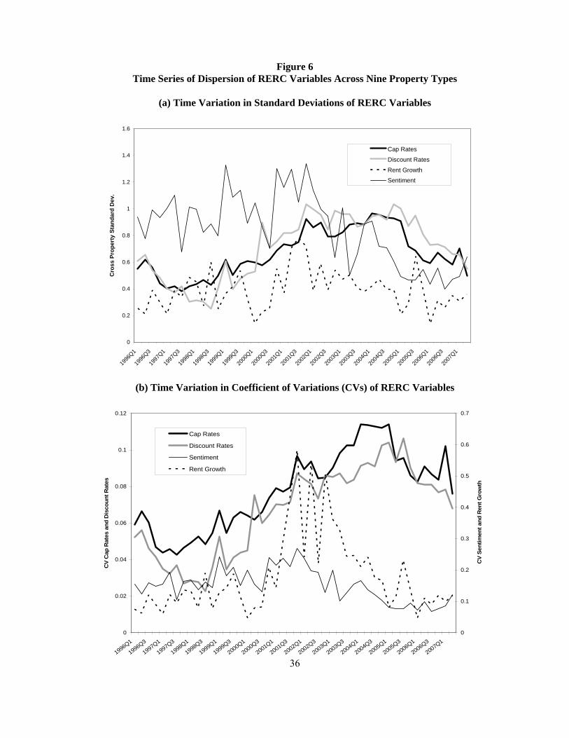
Figure 6 Time Series of Dispersion of RERC Variables Across Nine Property Types

(a) Time Variation in Standard Deviations of RERC Variables

0

0.2

0.4

0.6

0.8

1

1.2

1.4

1.6

1996

Q1

1996

Q3

1997

Q1

1997

Q3

1998

Q1

1998

Q3

1999

Q1

1999

Q3

2000

Q1

2000

Q3

2001

Q1

2001

Q3

2002

Q1

2002

Q3

2003

Q1

2003

Q3

2004

Q1

2004

Q3

2005

Q1

2005

Q3

2006

Q1

2006

Q3

2007

Q1

Cro

ss P

rope

rty

Stan

dard

Dev

.

Cap Rates

Discount Rates

Rent Growth

Sentiment

(b) Time Variation in Coefficient of Variations (CVs) of RERC Variables

0

0.02

0.04

0.06

0.08

0.1

0.12

1996Q1

1996Q3

1997Q1

1997Q3

1998Q1

1998Q3

1999Q1

1999Q3

2000Q1

2000Q3

2001Q1

2001Q3

2002Q1

2002Q3

2003Q1

2003Q3

2004Q1

2004Q3

2005Q1

2005Q3

2006Q1

2006Q3

2007Q1

CV

Cap

Rat

es a

nd D

isco

unt R

ates

0

0.1

0.2

0.3

0.4

0.5

0.6

0.7

CV

Sent

imen

t and

Ren

t Gro

wth

Cap Rates

Discount Rates

Sentiment

Rent Growth

36

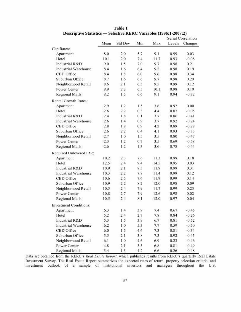
Table 1 Descriptive Statistics — Selective RERC Variables (1996:1-2007:2)

Mean Std Dev Min Max Levels ChangesCap Rates:

Apartment 8.0 2.0 5.7 9.1 0.99 0.03Hotel 10.1 2.0 7.4 11.7 0.93 -0.08Industrial R&D 9.0 1.5 7.0 9.7 0.98 0.21Industrial Warehouse 8.4 1.6 6.4 9.2 0.98 0.19CBD Office 8.4 1.8 6.0 9.6 0.98 0.34Suburban Office 8.7 1.6 6.6 9.7 0.98 0.29Neighborhood Retail 8.6 2.1 6.5 9.5 0.99 0.12Power Center 8.9 2.3 6.5 10.1 0.98 0.10Regional Malls 8.2 1.5 6.6 9.1 0.94 -0.32

Rental Growth Rates:Apartment 2.9 1.2 1.5 3.6 0.92 0.00Hotel 2.6 2.2 0.3 4.4 0.87 -0.05Industrial R&D 2.4 1.8 0.1 3.7 0.86 -0.41Industrial Warehouse 2.6 1.4 0.9 3.7 0.92 -0.24CBD Office 2.8 1.8 0.9 4.2 0.89 -0.28Suburban Office 2.6 2.2 0.4 4.1 0.93 -0.35Neighborhood Retail 2.7 1.0 1.5 3.5 0.80 -0.47Power Center 2.3 1.2 0.7 3.5 0.69 -0.58Regional Malls 2.6 1.2 1.3 3.6 0.78 -0.44

Required Unlevered IRR:Apartment 10.2 2.3 7.6 11.3 0.99 0.18Hotel 12.5 2.4 9.4 14.5 0.95 0.03Industrial R&D 10.9 2.1 8.3 11.9 0.99 0.31Industrial Warehouse 10.3 2.2 7.8 11.4 0.99 0.12CBD Office 10.6 2.5 7.6 11.9 0.99 0.14Suburban Office 10.9 2.2 8.2 12.0 0.98 0.09Neighborhood Retail 10.5 2.4 7.9 11.7 0.99 0.23Power Center 10.8 2.7 7.9 12.6 0.98 0.02Regional Malls 10.5 2.4 8.1 12.0 0.97 0.04

Investment Conditions:Apartment 6.3 1.4 3.9 7.4 0.67 -0.45Hotel 5.2 2.4 2.7 7.8 0.84 -0.26Industrial R&D 5.3 1.5 3.9 6.7 0.81 -0.52Industrial Warehouse 6.2 1.0 5.3 7.7 0.59 -0.50CBD Office 6.0 1.5 4.6 7.3 0.81 -0.34Suburban Office 5.5 2.1 3.8 7.3 0.92 -0.45Neighborhood Retail 6.1 1.0 4.6 6.9 0.23 -0.46Power Center 4.8 2.1 3.3 6.8 0.81 -0.49Regional Malls 5.4 1.3 4.2 6.6 0.26 -0.48

Serial Correlation

Data are obtained from the RERC’s Real Estate Report, which publishes results from RERC’s quarterly Real Estate Investment Survey. The Real Estate Report summarizes the expected rates of return, property selection criteria, and investment outlook of a sample of institutional investors and managers throughout the U.S.

37

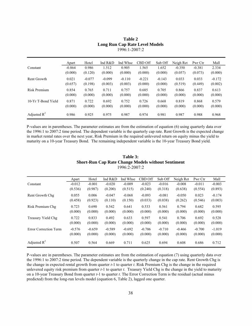
Table 2 Long Run Cap Rate Level Models

1996:1-2007:2

Apart Hotel Ind R&D Ind Whse CBD Off Sub Off Neigh Ret Pwr Ctr MallConstant -0.864 0.986 1.512 0.905 1.565 1.652 -0.350 -0.381 2.334

(0.000) (0.120) (0.000) (0.000) (0.000) (0.000) (0.057) (0.073) (0.000)

Rent Growth 0.021 -0.077 -0.099 -0.110 -0.221 -0.143 0.033 0.033 -0.172(0.657) (0.198) (0.003) (0.003) (0.000) (0.000) (0.519) (0.449) (0.002)

Risk Premium 0.854 0.765 0.711 0.757 0.685 0.705 0.866 0.837 0.613(0.000) (0.000) (0.000) (0.000) (0.000) (0.000) (0.000) (0.000) (0.000)

10-Yr T-Bond Yield 0.871 0.722 0.692 0.752 0.726 0.668 0.819 0.868 0.579(0.000) (0.000) (0.000) (0.000) (0.000) (0.000) (0.000) (0.000) (0.000)

Adjusted R2 0.986 0.925 0.975 0.987 0.974 0.981 0.987 0.988 0.968

P-values are in parentheses. The parameter estimates are from the estimation of equation (6) using quarterly data over the 1996:1 to 2007:2 time period. The dependent variable is the quarterly cap rate. Rent Growth is the expected change in market rental rates over the next year, Risk Premium in the required unlevered return on equity minus the yield to maturity on a 10-year Treasury Bond. The remaining independent variable is the 10-year Treasury Bond yield.

Table 3: Short-Run Cap Rate Change Models without Sentiment

1996:2-2007:2

Apart Hotel Ind R&D Ind Whse CBD Off Sub Off Neigh Ret Pwr Ctr MallConstant -0.012 -0.001 -0.020 -0.009 -0.023 -0.016 -0.008 -0.011 -0.003

(0.536) (0.987) (0.200) (0.515) (0.240) (0.318) (0.638) (0.554) (0.893)

Rent Growth Chg 0.055 0.006 -0.047 -0.068 -0.093 -0.081 -0.050 0.023 -0.174(0.458) (0.923) (0.110) (0.150) (0.033) (0.038) (0.262) (0.546) (0.003)

Risk Premium Chg 0.723 0.690 0.542 0.641 0.533 0.561 0.794 0.682 0.595(0.000) (0.000) (0.000) (0.000) (0.000) (0.000) (0.000) (0.000) (0.000)

Treasury Yield Chg 0.722 0.833 0.492 0.633 0.597 0.541 0.706 0.692 0.528(0.000) (0.000) (0.000) (0.000) (0.000) (0.000) (0.000) (0.000) (0.000)

Error Correction Term -0.576 -0.659 -0.589 -0.692 -0.706 -0.710 -0.466 -0.700 -1.019(0.000) (0.000) (0.000) (0.000) (0.000) (0.000) (0.000) (0.000) (0.000)

Adjusted R2 0.507 0.564 0.669 0.711 0.625 0.694 0.608 0.686 0.712

P-values are in parentheses. The parameter estimates are from the estimation of equation (7) using quarterly data over the 1996:1 to 2007:2 time period. The dependent variable is the quarterly change in the cap rate. Rent Growth Chg is the change in expected rental growth from quarter t-1 to quarter t. Risk Premium Chg is the change in the required unlevered equity risk premium from quarter t-1 to quarter t. Treasury Yield Chg is the change in the yield to maturity on a 10-year Treasury Bond from quarter t-1 to quarter t. The Error Correction Term is the residual (actual minus predicted) from the long-run levels model (equation 6, Table 2), lagged one quarter.

38

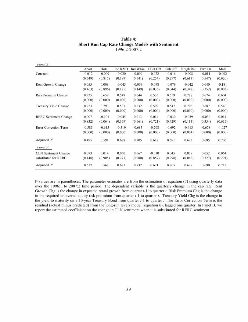
Table 4: Short Run Cap Rate Change Models with Sentiment

1996:2-2007:2

Panel A:Apart Hotel Ind R&D Ind Whse CBD Off Sub Off Neigh Ret Pwr Ctr Mall

Constant -0.012 -0.009 -0.020 -0.009 -0.022 -0.016 -0.008 -0.011 -0.002(0.549) (0.815) (0.189) (0.541) (0.254) (0.297) (0.613) (0.547) (0.920)

Rent Growth Change 0.055 0.008 -0.045 -0.069 -0.098 -0.079 -0.042 0.040 -0.181(0.463) (0.896) (0.125) (0.149) (0.035) (0.044) (0.342) (0.352) (0.003)

Risk Premium Change 0.725 0.659 0.549 0.644 0.535 0.559 0.788 0.674 0.604(0.000) (0.000) (0.000) (0.000) (0.000) (0.000) (0.000) (0.000) (0.000)

Treasury Yield Change 0.723 0.797 0.501 0.632 0.599 0.547 0.706 0.687 0.540(0.000) (0.000) (0.000) (0.000) (0.000) (0.000) (0.000) (0.000) (0.000)

RERC Sentiment Change 0.007 -0.101 -0.045 0.013 0.014 -0.030 -0.039 -0.030 0.014(0.832) (0.064) (0.159) (0.661) (0.721) (0.429) (0.113) (0.354) (0.635)

Error Correction Term -0.585 -0.613 -0.519 -0.683 -0.708 -0.692 -0.413 -0.678 -1.027(0.000) (0.000) (0.000) (0.000) (0.000) (0.000) (0.004) (0.000) (0.000)

Adjusted R2 0.495 0.591 0.678 0.705 0.617 0.691 0.623 0.685 0.706

Panel B:

CLN Sentiment Change 0.073 0.014 0.050 0.067 -0.010 0.045 0.078 0.052 0.064substituted for RERC (0.148) (0.905) (0.271) (0.080) (0.857) (0.298) (0.062) (0.327) (0.291)

Adjusted R2 0.517 0.568 0.671 0.732 0.621 0.705 0.628 0.690 0.712

P-values are in parentheses. The parameter estimates are from the estimation of equation (7) using quarterly data over the 1996:1 to 2007:2 time period. The dependent variable is the quarterly change in the cap rate. Rent Growth Chg is the change in expected rental growth from quarter t-1 to quarter t. Risk Premium Chg is the change in the required unlevered equity risk pre mium from quarter t-1 to quarter t. Treasury Yield Chg is the change in the yield to maturity on a 10-year Treasury Bond from quarter t-1 to quarter t. The Error Correction Term is the residual (actual minus predicted) from the long-run levels model (equation 6), lagged one quarter. In Panel B, we report the estimated coefficient on the change in CLN sentiment when it is substituted for RERC sentiment.

39

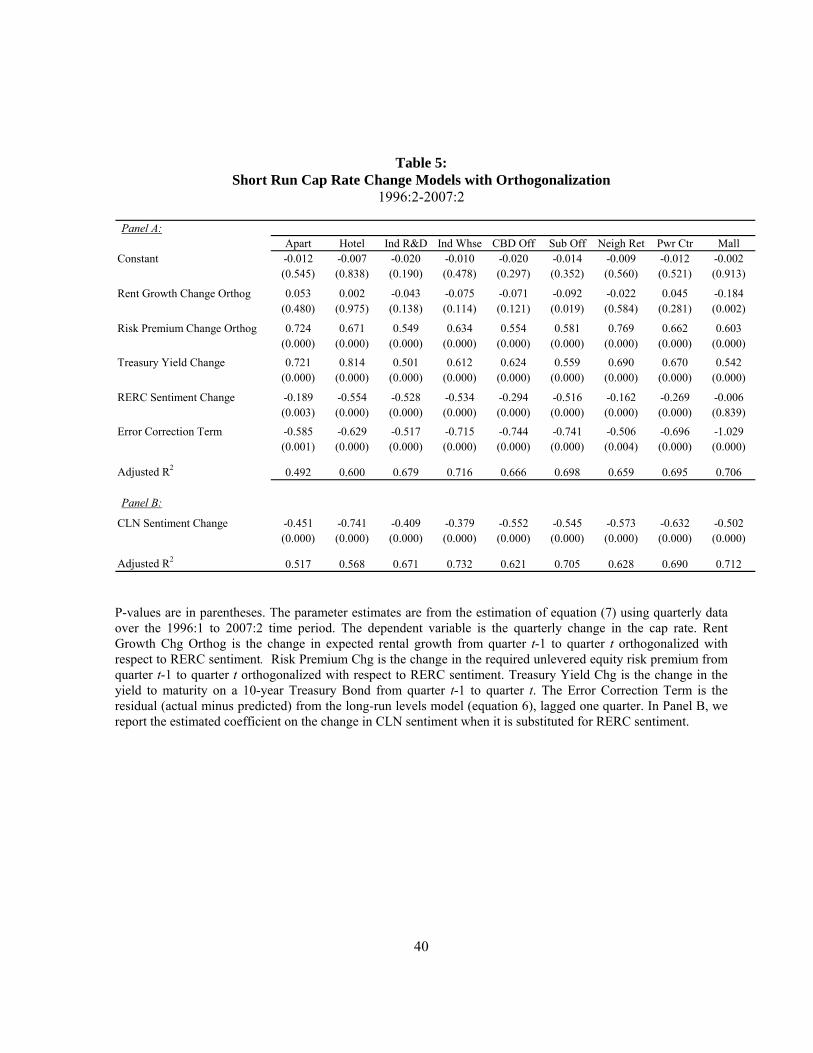
Table 5: Short Run Cap Rate Change Models with Orthogonalization

1996:2-2007:2

Panel A:Apart Hotel Ind R&D Ind Whse CBD Off Sub Off Neigh Ret Pwr Ctr Mall

Constant -0.012 -0.007 -0.020 -0.010 -0.020 -0.014 -0.009 -0.012 -0.002(0.545) (0.838) (0.190) (0.478) (0.297) (0.352) (0.560) (0.521) (0.913)

Rent Growth Change Orthog 0.053 0.002 -0.043 -0.075 -0.071 -0.092 -0.022 0.045 -0.184(0.480) (0.975) (0.138) (0.114) (0.121) (0.019) (0.584) (0.281) (0.002)

Risk Premium Change Orthog 0.724 0.671 0.549 0.634 0.554 0.581 0.769 0.662 0.603(0.000) (0.000) (0.000) (0.000) (0.000) (0.000) (0.000) (0.000) (0.000)

Treasury Yield Change 0.721 0.814 0.501 0.612 0.624 0.559 0.690 0.670 0.542(0.000) (0.000) (0.000) (0.000) (0.000) (0.000) (0.000) (0.000) (0.000)

RERC Sentiment Change -0.189 -0.554 -0.528 -0.534 -0.294 -0.516 -0.162 -0.269 -0.006(0.003) (0.000) (0.000) (0.000) (0.000) (0.000) (0.000) (0.000) (0.839)

Error Correction Term -0.585 -0.629 -0.517 -0.715 -0.744 -0.741 -0.506 -0.696 -1.029(0.001) (0.000) (0.000) (0.000) (0.000) (0.000) (0.004) (0.000) (0.000)

Adjusted R2 0.492 0.600 0.679 0.716 0.666 0.698 0.659 0.695 0.706

Panel B:

CLN Sentiment Change -0.451 -0.741 -0.409 -0.379 -0.552 -0.545 -0.573 -0.632 -0.502 (0.000) (0.000) (0.000) (0.000) (0.000) (0.000) (0.000) (0.000) (0.000) Adjusted R2 0.517 0.568 0.671 0.732 0.621 0.705 0.628 0.690 0.712

P-values are in parentheses. The parameter estimates are from the estimation of equation (7) using quarterly data over the 1996:1 to 2007:2 time period. The dependent variable is the quarterly change in the cap rate. Rent Growth Chg Orthog is the change in expected rental growth from quarter t-1 to quarter t orthogonalized with respect to RERC sentiment. Risk Premium Chg is the change in the required unlevered equity risk premium from quarter t-1 to quarter t orthogonalized with respect to RERC sentiment. Treasury Yield Chg is the change in the yield to maturity on a 10-year Treasury Bond from quarter t-1 to quarter t. The Error Correction Term is the residual (actual minus predicted) from the long-run levels model (equation 6), lagged one quarter. In Panel B, we report the estimated coefficient on the change in CLN sentiment when it is substituted for RERC sentiment.

40

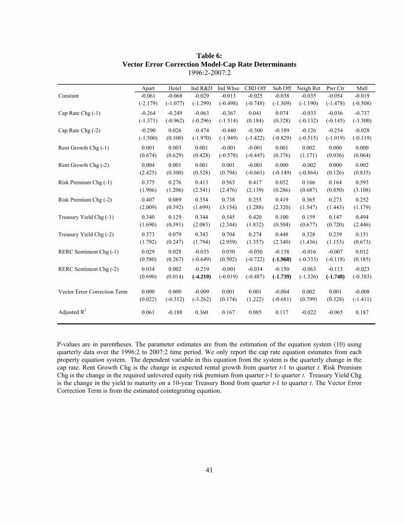
Table 6:

Vector Error Correction Model-Cap Rate Determinants 1996:2-2007:2

Apart Hotel Ind R&D Ind Whse CBD Off Sub Off Neigh Ret Pwr Ctr MallConstant -0.061 -0.068 -0.029 -0.013 -0.025 -0.038 -0.035 -0.054 -0.019

(-2.179) (-1.077) (-1.299) (-0.498) (-0.748) (-1.309) (-1.190) (-1.478) (-0.508)

Cap Rate Chg (-1) -0.264 -0.249 -0.063 -0.367 0.041 0.074 -0.033 -0.036 -0.737(-1.371) (-0.962) (-0.296) (-1.514) (0.184) (0.328) (-0.132) (-0.145) (-3.300)

Cap Rate Chg (-2) -0.290 0.026 -0.474 -0.440 -0.300 -0.189 -0.126 -0.254 -0.028(-1.500) (0.100) (-1.970) (-1.949) (-1.422) (-0.829) (-0.515) (-1.019) (-0.119)

Rent Growth Chg (-1) 0.001 0.003 0.001 -0.001 -0.001 0.001 0.002 0.000 0.000(0.674) (0.629) (0.428) (-0.578) (-0.445) (0.376) (1.171) (0.036) (0.064)

Rent Growth Chg (-2) 0.004 0.001 0.001 0.001 -0.001 0.000 -0.002 0.000 0.002(2.425) (0.300) (0.528) (0.794) (-0.661) (-0.149) (-0.864) (0.126) (0.835)

Risk Premium Chg (-1) 0.375 0.276 0.413 0.563 0.417 0.052 0.166 0.164 0.593(1.906) (1.206) (2.541) (2.476) (2.139) (0.286) (0.687) (0.850) (3.108)

Risk Premium Chg (-2) 0.407 0.089 0.334 0.738 0.255 0.419 0.365 0.273 0.252(2.009) (0.392) (1.699) (3.154) (1.288) (2.320) (1.547) (1.443) (1.179)

Treasury Yield Chg (-1) 0.340 0.129 0.344 0.545 0.420 0.100 0.159 0.147 0.494(1.690) (0.391) (2.083) (2.344) (1.832) (0.504) (0.677) (0.720) (2.446)

Treasury Yield Chg (-2) 0.373 0.079 0.343 0.704 0.274 0.448 0.328 0.239 0.151(1.792) (0.247) (1.794) (2.959) (1.357) (2.340) (1.436) (1.153) (0.673)

RERC Sentiment Chg (-1) 0.029 0.028 -0.035 0.030 -0.050 -0.158 -0.016 -0.007 0.012(0.580) (0.267) (-0.649) (0.502) (-0.722) (-1.968) (-0.333) (-0.118) (0.185)

RERC Sentiment Chg (-2) 0.034 0.002 -0.219 -0.001 -0.034 -0.150 -0.063 -0.113 -0.023(0.690) (0.014) (-4.210) (-0.019) (-0.487) (-1.739) (-1.326) (-1.748) (-0.383)

Vector Error Correction Term 0.000 0.000 -0.009 0.001 0.001 -0.004 0.002 0.001 -0.008(0.022) (-0.312) (-3.262) (0.174) (1.222) (-0.681) (0.799) (0.328) (-1.411)

Adjusted R2 0.061 -0.188 0.360 0.167 0.085 0.117 -0.022 -0.065 0.187

P-values are in parentheses. The parameter estimates are from the estimation of the equation system (10) using quarterly data over the 1996:2 to 2007:2 time period. We only report the cap rate equation estimates from each property equation system. The dependent variable in this equation from the system is the quarterly change in the cap rate. Rent Growth Chg is the change in expected rental growth from quarter t-1 to quarter t. Risk Premium Chg is the change in the required unlevered equity risk premium from quarter t-1 to quarter t. Treasury Yield Chg is the change in the yield to maturity on a 10-year Treasury Bond from quarter t-1 to quarter t. The Vector Error Correction Term is from the estimated cointegrating equation.

41

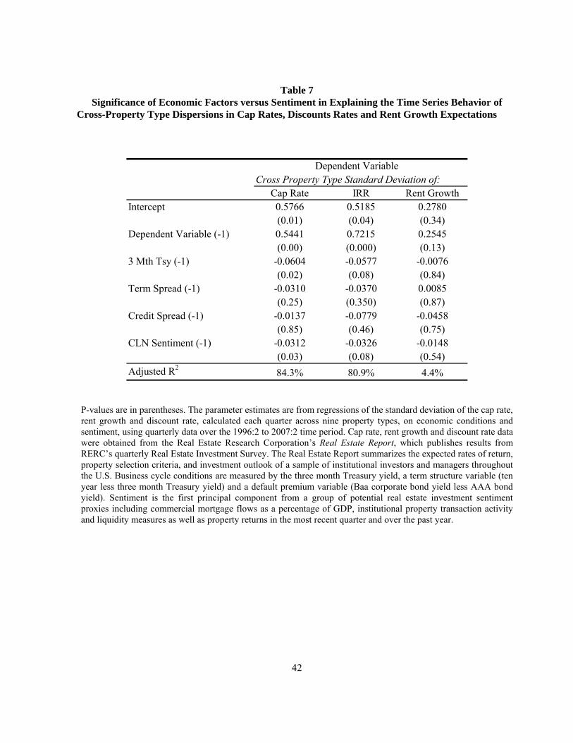
Table 7 Significance of Economic Factors versus Sentiment in Explaining the Time Series Behavior of

Cross-Property Type Dispersions in Cap Rates, Discounts Rates and Rent Growth Expectations

Dependent VariableCross Property Type Standard Deviation of:

Cap Rate IRR Rent GrowthIntercept 0.5766 0.5185 0.2780

(0.01) (0.04) (0.34)Dependent Variable (-1) 0.5441 0.7215 0.2545

(0.00) (0.000) (0.13)3 Mth Tsy (-1) -0.0604 -0.0577 -0.0076

(0.02) (0.08) (0.84)Term Spread (-1) -0.0310 -0.0370 0.0085

(0.25) (0.350) (0.87)Credit Spread (-1) -0.0137 -0.0779 -0.0458

(0.85) (0.46) (0.75)CLN Sentiment (-1) -0.0312 -0.0326 -0.0148

(0.03) (0.08) (0.54)Adjusted R2 84.3% 80.9% 4.4%

P-values are in parentheses. The parameter estimates are from regressions of the standard deviation of the cap rate, rent growth and discount rate, calculated each quarter across nine property types, on economic conditions and sentiment, using quarterly data over the 1996:2 to 2007:2 time period. Cap rate, rent growth and discount rate data were obtained from the Real Estate Research Corporation’s Real Estate Report, which publishes results from RERC’s quarterly Real Estate Investment Survey. The Real Estate Report summarizes the expected rates of return, property selection criteria, and investment outlook of a sample of institutional investors and managers throughout the U.S. Business cycle conditions are measured by the three month Treasury yield, a term structure variable (ten year less three month Treasury yield) and a default premium variable (Baa corporate bond yield less AAA bond yield). Sentiment is the first principal component from a group of potential real estate investment sentiment proxies including commercial mortgage flows as a percentage of GDP, institutional property transaction activity and liquidity measures as well as property returns in the most recent quarter and over the past year.

42