Investor Flows and the 2008 Boom/Bust in Oil Prices€¦ · · 2011-08-11Investor Flows and the...
36
Investor Flows and the 2008 Boom/Bust in Oil Prices Kenneth J. Singleton 1 August 10, 2011 1 Graduate School of Business, Stanford University, [email protected]. This research is the outgrowth of a survey paper I prepared for the Air Transport Association of America. I am grateful to Kristoffer Laursen for research assistance and to Kristoffer and Stefan Nagel for their comments.
Transcript of Investor Flows and the 2008 Boom/Bust in Oil Prices€¦ · · 2011-08-11Investor Flows and the...

Investor Flows and the 2008 Boom/Bust in Oil Prices
Kenneth J. Singleton1
August 10, 2011
1Graduate School of Business, Stanford University, [email protected]. This research is theoutgrowth of a survey paper I prepared for the Air Transport Association of America. I am gratefulto Kristoffer Laursen for research assistance and to Kristoffer and Stefan Nagel for their comments.

Abstract
This paper explores the impact of investor flows and financial market conditions on returns in
crude-oil futures markets. I begin by arguing that informational frictions and the associated
speculative activity may induce prices to drift away from “fundamental” values and show
increased volatility. This is followed by a discussion of the interplay between imperfect infor-
mation about real economic activity, including supply, demand, and inventory accumulation,
and speculative activity. Then, I present new evidence that there was an economically and
statistically significant effect of investor flows on futures prices, after controlling for returns in
US and emerging-economy stock markets, a measure of the balance-sheet flexibility of large
financial institutions, open interest, the futures/spot basis, and lagged returns on oil futures.
The intermediate-term growth rates of index positions and managed-money spread positions
had the largest impacts on futures prices. Moreover, my findings suggest that these effects
were through risk or informational channels distinct from changes in convenience yield.

1 Introduction
The dramatic rise and subsequent sharp decline in crude oil prices during 2008 has been
a catalyst for extensive debate about the roles of speculative trading activity in price
determination in energy markets.1 Many attribute these swings to changes in fundamentals of
supply and demand with the price effects and volatility actually moderated by the participation
of non-user speculators and passive investors in oil futures markets and other energy-related
derivatives.2 At the same time there is mounting evidence that the “financialization” of
commodity markets and the associated flows of funds into these markets from various categories
of investors have had substantial impacts on the drifts and volatilities of commodity prices.3
This paper builds upon the latter literature and undertakes an in depth analysis of the impact
of investor flows and financial market conditions on returns in crude-oil futures markets.
The prototypical dynamic models referenced in discussions of the oil boom (e.g., Hamilton
(2009a), Pirrong (2009)) have representative agent-types (producer, storage operator, com-
mercial consumer, etc.) and simplified forms of demand/supply uncertainty. Moreover, these
models, as well as the price-setting environment underlying Irwin and Sanders (2010)’s case
against a role for speculative trading, do not allow for learning under imperfect information,
heterogeneity of beliefs, and capital market and agency-related frictions that limit arbitrage
activity. As such, they abstract entirely from the consequent rational motives for many
categories of market participants to speculate in commodity markets based on their individual
circumstances and views about fundamental economic factors.
Detailed information about the origins of most of the open interest in OTC commodity
derivatives that could in principle shed light on the historical contributions of information-
and learning-based speculative activity is not publicly available. However, indirect inferences
suggest that traders’ investment strategies did impact prices. Tang and Xiong (2011) show
that, after 2004, agricultural commodities that are part of the GSCI and DJ-AIG indices
became much more responsive to shocks to a world equity index, changes in the U.S. dollar
exchange rate, and oil prices. These trends are stronger for those commodities that are
part of a major index than for other commodities. Tang and Xiong attribute their findings
to “spillover effects brought on by the increasing presence of index investors to individual
commodities (page 17).” Using proprietary data from the Commodity Futures Trading
1This debate is surely stimulated in part by the large costs that oil price booms and busts potentiallyimpose on the real economy. See, for example, Hooker (1996), Rotemberg and Woodford (1996), Hamilton(2003), and the survey by Sauter and Awerbuch (2003).
2The conceptual arguments and empirical evidence favoring this view are summarized in a recent Organi-zation of Economic Cooperation and Development report by Irwin and Sanders (2010).
3See, for example, Tang and Xiong (2011), Masters (2009), and Mou (2010).
1

250,000
350,000
450,000
550,000
650,000
750,000
850,000
$0.00
$25.00
$50.00
$75.00
$100.00
$125.00
$150.00
3-Ja
n-07
3-M
ar-0
7
3-M
ay-0
7
3-Ju
l-07
3-Se
p-07
3-N
ov-0
7
3-Ja
n-08
3-M
ar-0
8
3-M
ay-0
8
3-Ju
l-08
3-Se
p-08
3-N
ov-0
8
3-Ja
n-09
3-M
ar-0
9
3-M
ay-0
9
3-Ju
l-09
3-Se
p-09
3-N
ov-0
9
3-Ja
n-10
Cont
ract
s of
100
0's
of B
arre
ls
WTI
Pri
ce P
er B
arre
l
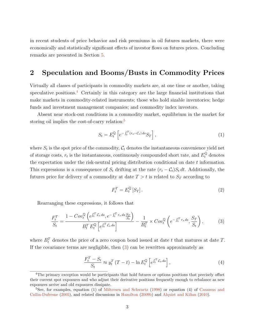
Figure 1: Commodity index long positions inferred from the CIT reports (dashed line, rightsale) plotted against the front-month NYMEX WTI futures price (solid line, left scale).
Commission (CFTC), Buyuksahin and Robe (2011) link increased high-frequency correlations
among equity and commodity returns to trading patterns of hedge funds. Less formally,
Masters (2009) imputes flows into crude oil positions by index investors using the CFTC’s
commodity index trader (CIT ) reports. The imputed index long positions based on his
methodology (Figure 1), displayed against the near-contract forward price of WTI crude
oil, shows a strikingly high degree of comovement. Additionally, Mou (2010) documents
substantial impacts on futures prices of the “roll strategies” employed by index funds, and
finds a link between the implicit transactions costs born by index investors and the level of
speculative capital deployed to “front run” these rolls.
To interpret these as well as my own empirical findings, I argue in Section 2 that
informational frictions (and the associated speculative activity) that can lead prices to drift
away from “fundamental” values, were likely to have been present in commodity markets.
Section 3 discusses the interplay between imperfect information about real economic activity,
including supply, demand, and inventory accumulation, and speculative activity. Section 4
presents new evidence that, even after controlling for many of the other conditioning variables
2
in recent students of price behavior and risk premiums in oil futures markets, there were
economically and statistically significant effects of investor flows on futures prices. Concluding
remarks are presented in Section 5.
2 Speculation and Booms/Busts in Commodity Prices
Virtually all classes of participants in commodity markets are, at one time or another, taking
speculative positions.4 Certainly in this category are the large financial institutions that
make markets in commodity-related instruments; those who hold sizable inventories; hedge
funds and investment management companies; and commodity index investors.
Absent near stock-out conditions in a commodity market, equilibrium in the market for
storing oil implies the cost-of-carry relation:5
St = EQt
[e−
∫ Tt (rs−Cs) dsST
], (1)
where St is the spot price of the commodity, Ct denotes the instantaneous convenience yield net
of storage costs, rt is the instantaneous, continuously compounded short rate, and EQt denotes
the expectation under the risk-neutral pricing distribution conditional on date t information.
This expressions is a consequence of St drifting at the rate (rt − Ct)St dt. Additionally, the
futures price for delivery of a commodity at date T > t is related to ST according to
F Tt = EQ
t [ST ] . (2)
Rearranging these expressions, it follows that
F Tt
St=
1− CovQt(e∫ Tt Cs ds, e−
∫ Tt rs ds ST
St
)BTt E
Qt
[e∫ Tt Cs ds
] − 1
BTt
× CovQt(e−
∫ Tt rs ds,
STSt
), (3)
where BTt denotes the price of a zero coupon bond issued at date t that matures at date T .
If the covariance terms are negligible, then (3) can be rewritten approximately as
F Tt − StSt
≈ yTt (T − t)− lnEQt
[e∫ Tt Cs ds
], (4)
4The primary exception would be participants that hold futures or options positions that precisely offsettheir current spot exposures and who adjust their derivative positions frequently enough to rebalance as newexposures arrive and old exposures dissipate.
5See, for examples, equation (1) of Miltersen and Schwartz (1998) or equation (4) of Casassus andCollin-Dufresne (2005), and related discussions in Hamilton (2009b) and Alquist and Kilian (2010).
3
where yTt is the continuously compounded yield on a zero of maturity (T − t) periods. This
is the multi-period counterpart to the standard expression of the futures basis in terms of
foregone interest and convenience yield. In the presence of stochastic interest rates and
convenience yields, the multiperiod covariances between r and C impact the relationship
between F Tt and St according to (3).
Most of the extant model-based interpretations of the oil price boom focus on representative
risk-neutral producers and refiners and arrive at a similar expression with the expectation
EQt replaced by EP
t , the expectation of market participants under the historical distribution.
The perfect-foresight model of Hamilton (2009a), for instance, leads to a special case of a
discrete-time counterpart of (1) without the expectation operator (since there is no uncertainty
about future oil prices, inventory accumulations, or supply). If refiners and investors are risk
averse, or if they face capital constraints that lead them to behave effectively as if they are
risk averse, then (1) is the appropriate starting point for discussing speculation.
Implicit in (1) and (2) are the risk premiums that market participants demand when
trading commodities in futures and spot markets. Define the market risk premium as
RP Tt ≡
(EQt [ST ]− EP
t [ST ]), for T > t. Further, consider a short time interval [t, τ ] over
which r and C are approximately constant. Then (3) implies that
EPt [Sτ ]− St
St− yτt ≈ Ct −RP τ
t . (5)
Thus, expected excess returns in the spot commodity market depend on both convenience
yields and risk premiums. The same will in general be true of expected excess returns in the
futures market, which are percentage changes in the price of a future contract, adjusted for
roll dates (see the Appendix for details).
To sustain the pricing relation (3) and it approximate simplification (5) in equilibrium,
it is not necessary that participants in the spot and futures markets, or those refining or
holding inventories of crude oil, be one and the same individual.6 It follows that: (i) Spot
prices are influenced not only by current oil market and macroeconomic conditions, but also
by investors’ expectations about future economic activity. (ii) Supply and demand pressures
in the futures and commodity swap markets will in general affect prices in the spot market.
Indeed, these relationships are fully consistent with price discovery taking place in either
the futures, the cash, or the commodity swap markets, or in all three. (iii) Risk premiums
6In particular, the claim that “index fund investors ... only participated in futures markets... In order toimpact the equilibrium price of commodities in the cash market, index investors would have to take deliveryand/or buy quantities in the cash market and hold these inventories off of the market. (ISOECD, page 8)” isnot true in the economic environment considered here.
4
will typically change over time as investors’ willingness to bear risk changes. As I discuss in
more depth below, the capacity of financial institutions to bear risk also changes over time,
and this also may affect equilibrium futures and spot prices. (iv) Higher-order moments of
prices and yields in financial markets also affect spot, futures, and swap prices through risk
premiums and precautionary demands.
In addition these pricing relationships accommodate the possibility that investors hold
different beliefs about the future course of economic events that impinge on commodity
prices, and hence that there is not a representative investor in commodity markets. With
the introduction of heterogeneity in beliefs, and absent risk aversion, one might naturally
focus on the cross-investor average expectation of future spot prices in expressions like (5).
However, when agents find it optimal to forecast the forecasts of others, the law of iterated
expectations no longer applies, and forward prices are the average of investors expected future
spot price plus an average across the forecast errors of the heterogeneously informed agents.
That is, averaging across investors will typically give an expression similar to∫iEi Pt [Sτ ]− StSt
− yτt ≈ C̃t − R̃Pτ
t + Eτt , (6)
where i indexes investors and the additional term Eτt captures the effects of forecast errors
and/or limits to arbitrage on spot and futures price determination.7
There is likely to be some disagreement among market participants about virtually every
source of fundamental risk, including the future of global demands, the prospects for supply,
future financing costs, etc. Saporta, Trott, and Tudela (2009) document large errors in
forecasting demand for oil, typically on the side of under estimation of demand and mostly
related to the non-OECD Asia and the Middle East regions. Additionally, they document
substantial revisions to forecasts of market tightness, based on data reported by the U.S.
Energy Information Administration (EIA), especially during 2007.8 The International Energy
Agency (IEA (2009)) points to substantial revisions to their monthly estimates of demands
for the U.S. and, regarding non-OECD inventories, IEA (2008a) observes that “detailed
inventory data [for China] continues to test observers’ powers of deduction. As we have
repeatedly stressed in this report, these data are key to any assessment of underlying demand
7See Xiong and Yan (2010) and Nimark (2009) for formal derivations of terms analogous to E in thecontext of term structure models.
8Market tightness is defined as total consumption (excluding stocks) minus the sum of non-OPEC andOPEC production. After comparing news about, and revisions in forecasts of, supply and demand for oilduring 2008, these authors conclude that “Based on the news about the balance of demand and supply in2008 ... it seems that one can justify neither the rise in prices in the first half of 2008, nor the fall in prices inthe second half (page 222).”
5
5.00
7.00
9.00
11.00
13.00
15.00
17.00
60.00
80.00
100.00
120.00
140.00
160.00
on of 1
‐Year A
head
Oil‐Price Forecasts
Price/Ba
rrel ($
)WTI Price
Dispersion of Forecasts
‐1.00
1.00
3.00
5.00
7.00
9.00
11.00
13.00
15.00
17.00
0.00
20.00
40.00
60.00
80.00
100.00
120.00
140.00
160.00
9‐Jan‐07
9‐Mar‐07
9‐May‐07
9‐Jul‐0
7
9‐Sep‐07
9‐Nov‐07
9‐Jan‐08
9‐Mar‐08
9‐May‐08
9‐Jul‐0
8
9‐Sep‐08
9‐Nov‐08
9‐Jan‐09
9‐Mar‐09
9‐May‐09
9‐Jul‐0
9
9‐Sep‐09
9‐Nov‐09
9‐Jan‐10
Dispersio
n of 1‐ Year A
head
Oil‐Price Forecasts
Price/Ba
rrel ($
)WTI Price
Dispersion of Forecasts
a
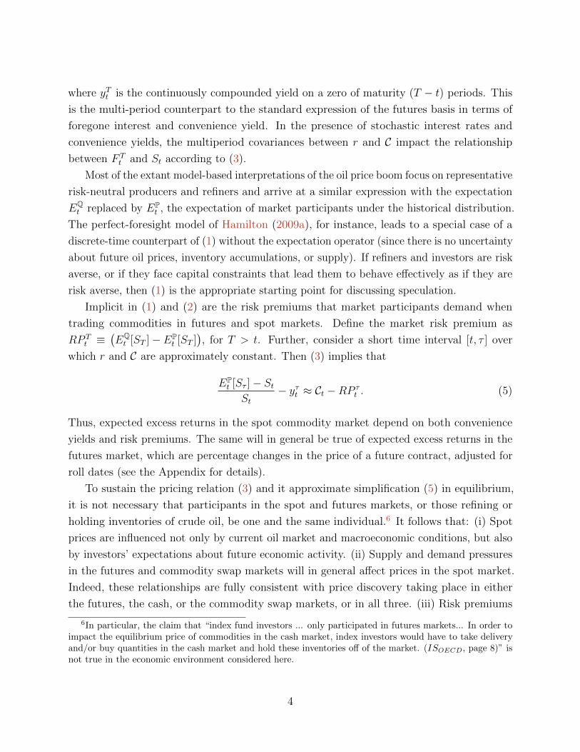
Figure 2: The front-month NYMEX WTI futures price (solid line, left scale) plotted againstthe cross-sectional dispersion of forecasts of oil prices one-year ahead by the professionalssurveyed by Consensus Economics (squares, right scale).
trends... (page 15)” Sornette, Woodard, and Zhou (2008) document significant differences
in the total world supplies for liquid fuels published by the IEA and the EIA, particularly
from 2006 until 2008. The timeliness of non-OECD data is highly variable (IEA), and OPEC
quotas and measured production levels are quite vague (Hamilton (2009b)).
Direct evidence on the extent of disagreement about future oil prices on the part of
professional market participants comes from comparing the patterns in the cross-sectional
standard deviations of the one-year ahead forecasts of oil prices by the professionals surveyed
by Consensus Economics.9 Larger values of this dispersion measure correspond to greater
disagreement among the professional forecasters surveyed. Figure 2 shows a strong positive
correlation between the degree of disagreement among forecasters and the level of the WTI
oil price. This comovement is consistent with the positive relationship between price drift
and dispersion in investors beliefs found in theory and documented in equity markets.
How might this heterogeneity of beliefs impact oil prices? In a “rational expectations”
9Consensus Economics surveys over thirty of (in their words) “the world’s most prominent commodityforecasters” and asks for their forecasts of oil prices in the future. The series plotted in Figure 2 is thecross-forecaster standard deviation for each month of their reported forecasts. I am grateful to the IMF forproviding this series, as reported in their World Economic Forum.
6
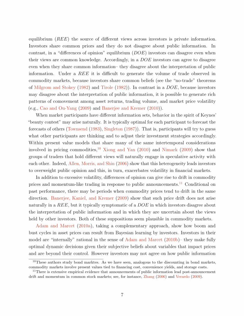
equilibrium (REE) the source of different views across investors is private information.
Investors share common priors and they do not disagree about public information. In
contrast, in a “differences of opinion” equilibrium (DOE) investors can disagree even when
their views are common knowledge. Accordingly, in a DOE investors can agree to disagree
even when they share common information– they disagree about the interpretation of public
information. Under a REE it is difficult to generate the volume of trade observed in
commodity markets, because investors share common beliefs (see the “no-trade” theorems
of Milgrom and Stokey (1982) and Tirole (1982)). In contrast in a DOE, because investors
may disagree about the interpretation of public information, it is possible to generate rich
patterns of comovement among asset returns, trading volume, and market price volatility
(e.g., Cao and Ou-Yang (2009) and Banerjee and Kremer (2010)).
When market participants have different information sets, behavior in the spirit of Keynes’
“beauty contest” may arise naturally. It is typically optimal for each participant to forecast the
forecasts of others (Townsend (1983), Singleton (1987)). That is, participants will try to guess
what other participants are thinking and to adjust their investment strategies accordingly.
Within present value models that share many of the same intertemporal considerations
involved in pricing commodities,10 Xiong and Yan (2010) and Nimark (2009) show that
groups of traders that hold different views will naturally engage in speculative activity with
each other. Indeed, Allen, Morris, and Shin (2006) show that this heterogeneity leads investors
to overweight public opinion and this, in turn, exacerbates volatility in financial markets.
In addition to excessive volatility, differences of opinion can give rise to drift in commodity
prices and momentum-like trading in response to public announcements.11 Conditional on
past performance, there may be periods when commodity prices tend to drift in the same
direction. Banerjee, Kaniel, and Kremer (2009) show that such price drift does not arise
naturally in a REE, but it typically symptomatic of a DOE in which investors disagree about
the interpretation of public information and in which they are uncertain about the views
held by other investors. Both of these suppositions seem plausible in commodity markets.
Adam and Marcet (2010a), taking a complementary approach, show how boom and
bust cycles in asset prices can result from Bayesian learning by investors. Investors in their
model are “internally” rational in the sense of Adam and Marcet (2010b)– they make fully
optimal dynamic decisions given their subjective beliefs about variables that impact prices
and are beyond their control. However investors may not agree on how public information
10These authors study bond marktes. As we have seen, analogous to the discounting in bond markets,commodity markets involve present values tied to financing cost, convenience yields, and storage costs.
11There is extensive empirical evidence that announcements of public information lead post-announcementdrift and momentum in common stock markets; see, for instance, Zhang (2006) and Verardo (2009).
7
about fundamentals translate into a specific price level. Nor do investors know the utility
weights that other investors assign to specific economic events. For both of these reasons
internally rational investors try to infer from market prices information about fundamental
economic variables and the end result is not a REE. They show that a model of stock price
formation embodying these features produces boom/bust cycles in stock prices that match
those experienced historically.
Three implications of this literature, particularly as they relate to the roles of speculation
in commodity markets, warrant emphasis. First, it is not necessary for investors with hetero-
geneous beliefs to have private information in order for their actions to impact commodity
prices. Rather, so long as they have differences of opinion about the interpretation of public
information and find it useful to learn from past prices, then their actions can induce higher
volatility, price drift, and booms and busts in prices. Second, the documented comovement
among futures prices on commodities that are and are not in an index, or among spot prices
across markets with and without associated futures contracts, is not evidence against an
important role for speculation underlying this comovement.12 Participants in all commodity
markets should find it optimal to condition on prices in other markets when drawing inferences
about future spot prices, and this includes wholesalers and speculators.13
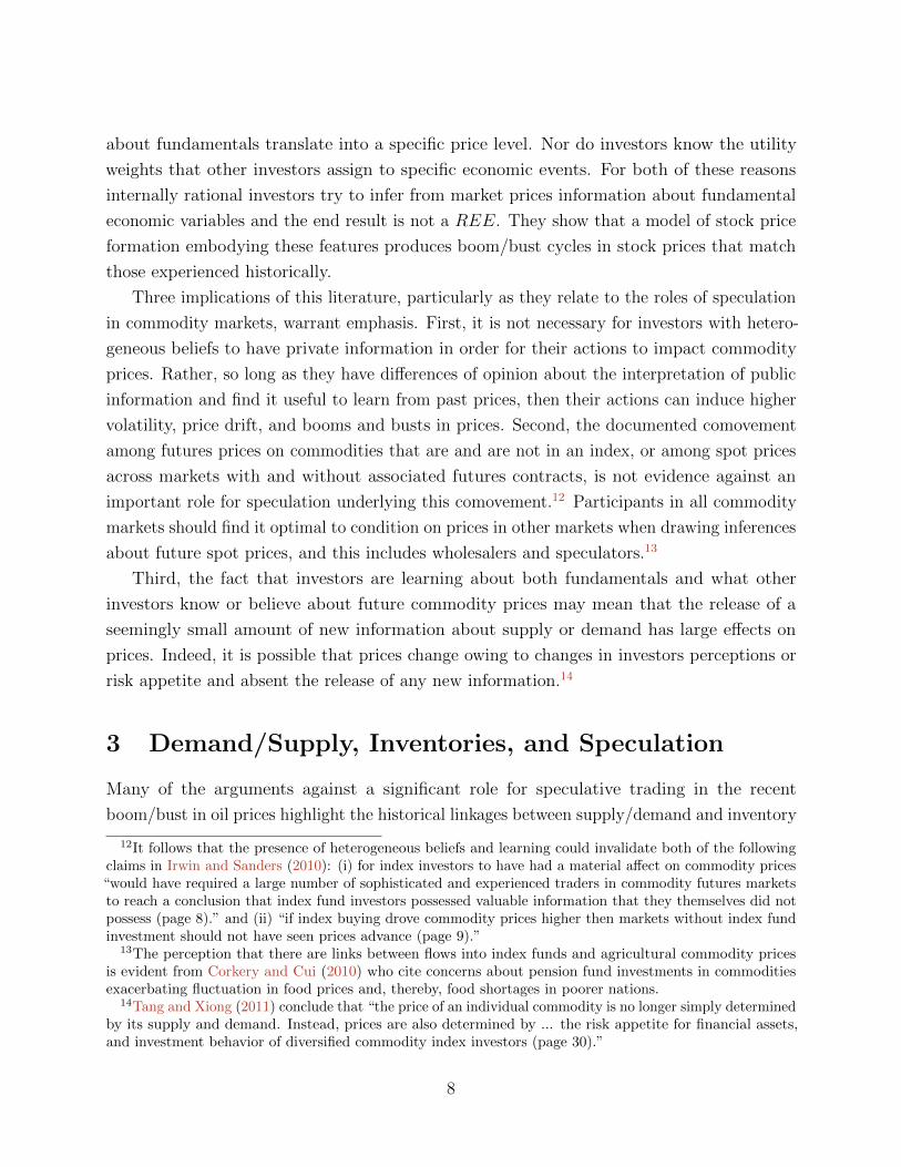
Third, the fact that investors are learning about both fundamentals and what other
investors know or believe about future commodity prices may mean that the release of a
seemingly small amount of new information about supply or demand has large effects on
prices. Indeed, it is possible that prices change owing to changes in investors perceptions or
risk appetite and absent the release of any new information.14
3 Demand/Supply, Inventories, and Speculation
Many of the arguments against a significant role for speculative trading in the recent
boom/bust in oil prices highlight the historical linkages between supply/demand and inventory
12It follows that the presence of heterogeneous beliefs and learning could invalidate both of the followingclaims in Irwin and Sanders (2010): (i) for index investors to have had a material affect on commodity prices“would have required a large number of sophisticated and experienced traders in commodity futures marketsto reach a conclusion that index fund investors possessed valuable information that they themselves did notpossess (page 8).” and (ii) “if index buying drove commodity prices higher then markets without index fundinvestment should not have seen prices advance (page 9).”
13The perception that there are links between flows into index funds and agricultural commodity pricesis evident from Corkery and Cui (2010) who cite concerns about pension fund investments in commoditiesexacerbating fluctuation in food prices and, thereby, food shortages in poorer nations.
14Tang and Xiong (2011) conclude that “the price of an individual commodity is no longer simply determinedby its supply and demand. Instead, prices are also determined by ... the risk appetite for financial assets,and investment behavior of diversified commodity index investors (page 30).”
8
$0$15$30$45$60$75$90
$105$120$135$150
260 270 280 290 300 310 320 330 340 350 360 370 380
Weekly U.S. Crude Oil Inventory Excluding Strategic Petroleum Reserve (Millions of Barrels )
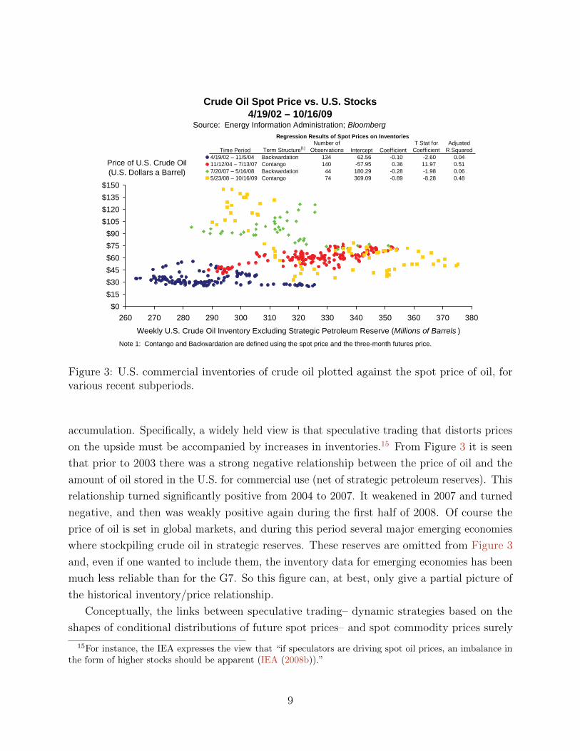
Crude Oil Spot Price vs. U.S. Stocks4/19/02 – 10/16/09
Source: Energy Information Administration; Bloomberg
Note 1: Contango and Backwardation are defined using the spot price and the three-month futures price.
Price of U.S. Crude Oil(U.S. Dollars a Barrel)
Regression Results of Spot Prices on Inventories
Time Period Term Structure[1]Number of
Observations Intercept CoefficientT Stat for
CoefficientAdjusted
R Squared4/19/02 – 11/5/04 Backwardation 134 62.56 -0.10 -2.60 0.0411/12/04 – 7/13/07 Contango 140 -57.95 0.36 11.97 0.517/20/07 – 5/16/08 Backwardation 44 180.29 -0.28 -1.98 0.065/23/08 – 10/16/09 Contango 74 369.09 -0.89 -8.28 0.48
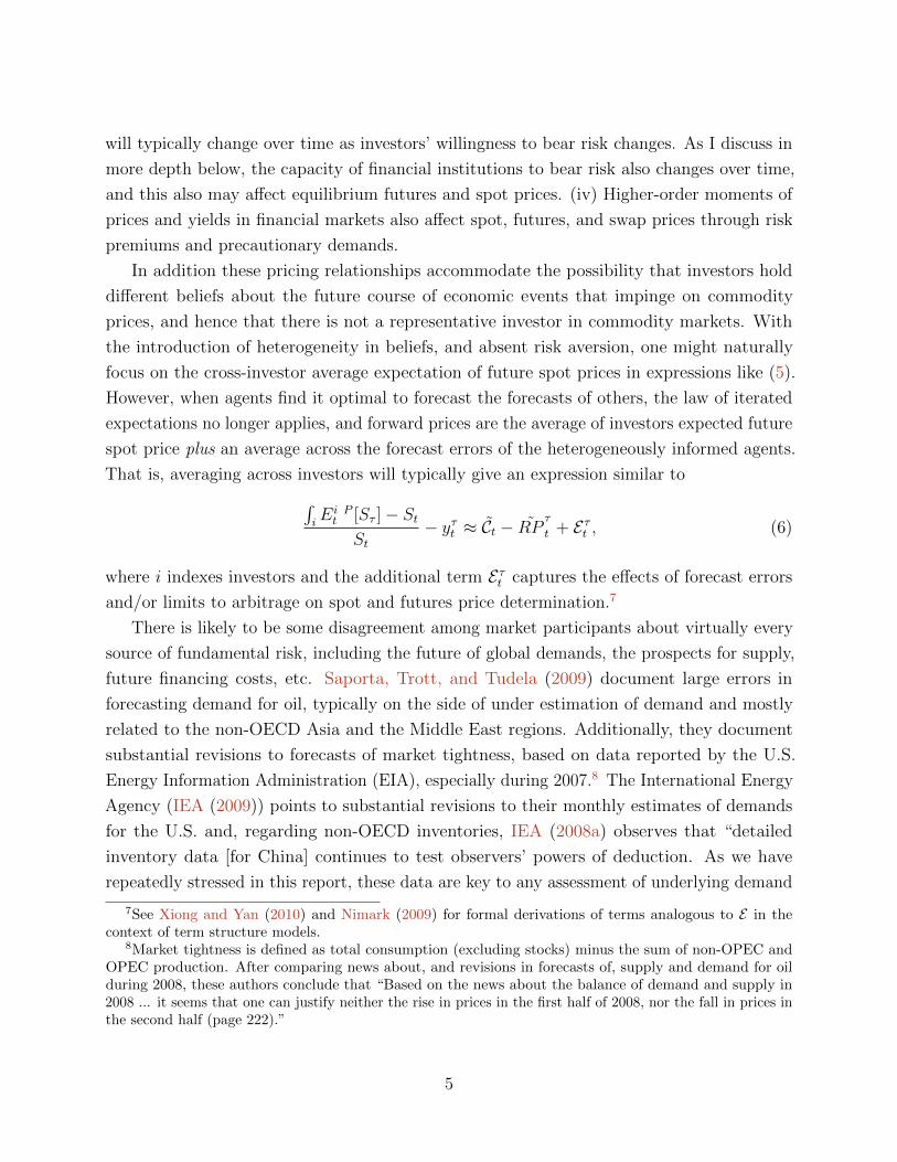
Figure 3: U.S. commercial inventories of crude oil plotted against the spot price of oil, forvarious recent subperiods.
accumulation. Specifically, a widely held view is that speculative trading that distorts prices
on the upside must be accompanied by increases in inventories.15 From Figure 3 it is seen
that prior to 2003 there was a strong negative relationship between the price of oil and the
amount of oil stored in the U.S. for commercial use (net of strategic petroleum reserves). This
relationship turned significantly positive from 2004 to 2007. It weakened in 2007 and turned
negative, and then was weakly positive again during the first half of 2008. Of course the
price of oil is set in global markets, and during this period several major emerging economies
where stockpiling crude oil in strategic reserves. These reserves are omitted from Figure 3
and, even if one wanted to include them, the inventory data for emerging economies has been
much less reliable than for the G7. So this figure can, at best, only give a partial picture of
the historical inventory/price relationship.
Conceptually, the links between speculative trading– dynamic strategies based on the
shapes of conditional distributions of future spot prices– and spot commodity prices surely
15For instance, the IEA expresses the view that “if speculators are driving spot oil prices, an imbalance inthe form of higher stocks should be apparent (IEA (2008b)).”
9
more complex than what emerges from models with static (non-forward looking or strategic)
demands on the part of a homogenous class of agents. In a dynamic uncertain environment,
time-varying expectations and volatility influence optimal inventory behavior. For instance,
Pirrong (2009) shows that in a model with time-varying volatility, but otherwise similar
features to Hamilton’s framework, there is not a stable relationship between inventories and
prices and that a positive inventory-price relationship may arise as a consequence of increased
demand- or supply-side uncertainty. Thus, there is not an unambiguously positive theoretical
relationship between changes in prices and inventories.
Equally importantly, the impact of inventory adjustments on the volatility of prices
depends critically on what one assumes about the nature of uncertainty about supply and
demand. Many storage models (e.g., Deaton and Laroque (1996)) assume that, subsequent
to a surprise change in inventories induced by a shock to demand, inventories revert to a
long-run mean. It is this response pattern that led Verleger (2010), among others, to expect
inventory adjustments to have a stabilizing effect on oil prices. However, these models of
storage cannot simultaneously explain the high degree of persistence in oil prices and the
high level of oil price volatility over the past 30 years (Dvir and Rogoff (2009)).
Arbitrageurs (those who store to make a profit from price changes) are confronted with
two opposing implications of a positive income or demand shock. The price of oil increases
and there is a drop in effective availability, both of which encourage a reduction in optimal
storage. On the other hand, the persistent nature of aggregate demand means that both
income and prices are expected to be higher in the future. Dvir and Rogoff (2009) show
that when growth has a trend component, the expectation that prices will be higher in the
future encourages an increase in inventories and this effect dominates the reduction in storage
induced by the immediate post-shock increase in prices. On balance, storage (by arbitrageurs,
refiners or consumers) may amplify the effects of demand shocks on prices.16 Aguiar and
Gopinath (2007) argue that shocks to growth contribute more to variability in output in
emerging than in developed economies.
At the core of many demand-based explanations for oil prices is the view that inelastic
demand, combined with a relatively steeply sloped supply curve, implied that small changes
in demand translated into large changes in prices, both on the upside and downside of the
boom/bust. This same reasoning implies that small changes in strategic inventory positions
can also have large changes in prices. Once expectations-based behavior is introduced, optimal
inventory management can potentially further amplify the effects of differences of opinion
16While this amplification mechanism has some characteristics of the precautionary demand studied byPirrong, the economic mechanism underlying it is not driven by uncertainty about demand, but rather byexpectations of rising prices.
10

200
250
300
350
400
450
Jan-04 Jan-05 Jan-06 Jan-07 Jan-08 Jan-09
-$8
-$6
-$4
-$2
$0
$2
$4
$6
U.S. Crude Oil Ending Stocks excl. SPR
M2 – M4
U.S. Crude Inventory Level excl. SPR vs. WTI Contango1/5/04 – 10/23/09
Source: Energy Information Administration; Bloomberg(Millions of Barrels )
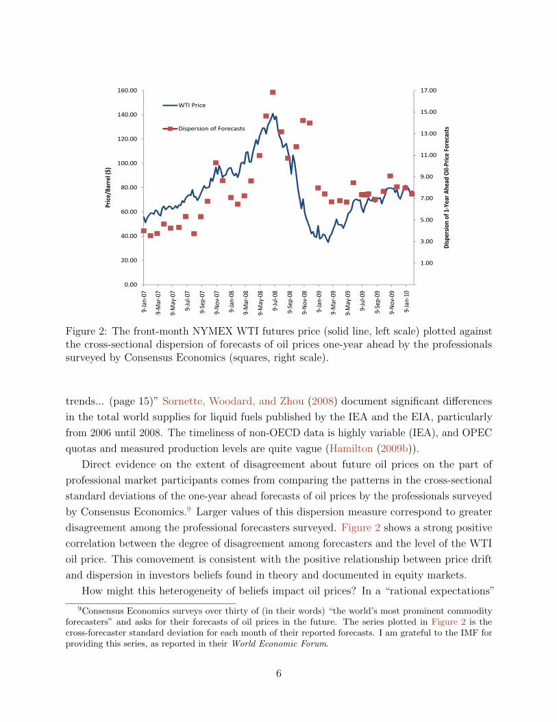
Figure 4: U.S. Commercial Inventories of Crude Oil Plotted Against the Spread BetweenTwo-Month and Four-Month Futures Prices
and learning on commodity prices.
Figure 4 plots the level of non-strategic U.S. crude oil inventories against the spread
between the futures prices for two- and four-month contracts (M2 −M4, inverted scale).
Spreads that are above the zero line occur when the futures market is in contango, and spreads
below this line indicate backwardation. There is a clear tendency throughout the period of
2004 through 2009 for inventories to increase when the futures market is in contango.17 A
notable feature of Figure 4 that seems consistent with the an amplification effect of strategic
behavior based on expected future prices is that, at least from 2007 onwards, steepening
and flattening of the forward curve preceded changes in inventories: a steeper forward curve
anticipated accumulations of inventories.
4 Investor Flows and Oil Prices
Teasing out the relative contributions of the risks associated with fundamental factors in
demand and supply through the channels encompassed in models such those of Hamilton
(2009a) and Pirrong (2009) from the effects of price drift owing to learning and speculation
17These patterns are even stronger when inventory levels from Cushing or Padd2 are used.
11

5
10
15
20
25
30
35
40
45Oil Std/GDP Std
0
5
10
15
20
25
30
35
40
45
February‐07
April‐07
June
‐07
August‐07
Octob
er‐07
Decem
ber‐07
February‐08
April‐08
June
‐08
August‐08
Octob
er‐08
Decem
ber‐08
February‐09
April‐09
June
‐09
August‐09
Octob
er‐09
Decem
ber‐09
February‐10
Oil Std/GDP Std
Figure 5: Ratio of the dispersions in forecasts for the price of oil and world economic growth(real GDP growth).
based on differences of opinion will require much richer structural models than have heretofore
been examined. In an attempt to provide some guidance to such endeavors, the remainder of
this paper explores the historical correlations between differences of opinion, trader flows,
and excess returns in oil markets, particularly for the 2008/09 boom and bust.
The comovement of the price of oil and the dispersion of forecasts of this price documented
in Figure 2 suggests that professional participants in this market held different views and
that these differences of opinion increased during the boom. Of relevance to the subsequent
discussion is whether this increase in dispersion coincided with increased dispersion in forecasts
of world economic growth. Some evidence on this question is provided in Figure 5 which
plots the ratio of the forecast dispersion for the price of oil to the corresponding dispersion of
forecasts of growth for the world economy.18 At least relative to the dispersion in opinions
about world economic growth, there was something special about oil markets during 2008.
Dispersion in views about economic growth did not rise substantially from its mid-2008 value
until the spring of 2009 when the financial crisis was more pronounced.
18For the purpose of these calculations the world is considered to be the G7 plus Brazil, China, India,Mexico, and Russia. I am grateful to the IMF for providing me with these dispersion measures.
12
4.1 What Is Known About Investor Flows and Commodity Prices?
Of particular interest to policy makers and academics alike is the question of whether
the growth in index investing– exposure to commodities through index-linked products–
contributed to price volatility, a higher level of oil prices and greater disagreement among
market participants about the future course of oil prices. It seems reasonable to presume
that the growth in index investing affected the trading strategies of at least some other large
investors. Buyuksahin, Haigh, Harris, Overdahl, and Robe (2008), for instance, argue that
prior to the early 2000’s, the prices of long- and short-dated futures contracts behaved as if
these contracts were traded in segmented markets. They find that, since the middle of 2004,
the prices of one- and two-year futures have become cointegrated with the nearby contract.
No doubt related to this closer integration of futures along the maturity spectrum are the
increased trading activities of hedge funds engaged in spread trades (Buyuksahin, Haigh,
Harris, Overdahl, and Robe (2008)) and the incentives for index-fund managers to purchase
longer-dated exposures through futures when the market is in contango. Very little is known
publicly about the degree to which different groups of commodity investors were effectively
trading against each other, either based on revealed positions of classes of investors, observed
order flow, or by following momentum strategies.19
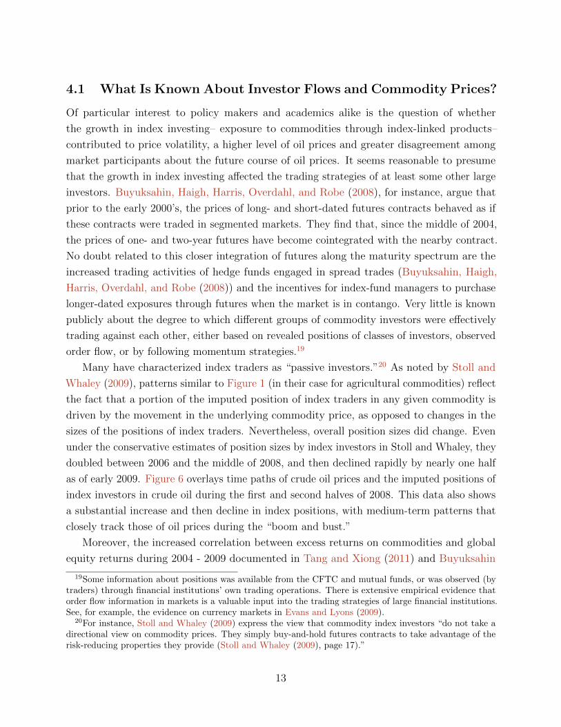
Many have characterized index traders as “passive investors.”20 As noted by Stoll and
Whaley (2009), patterns similar to Figure 1 (in their case for agricultural commodities) reflect
the fact that a portion of the imputed position of index traders in any given commodity is
driven by the movement in the underlying commodity price, as opposed to changes in the
sizes of the positions of index traders. Nevertheless, overall position sizes did change. Even
under the conservative estimates of position sizes by index investors in Stoll and Whaley, they
doubled between 2006 and the middle of 2008, and then declined rapidly by nearly one half
as of early 2009. Figure 6 overlays time paths of crude oil prices and the imputed positions of
index investors in crude oil during the first and second halves of 2008. This data also shows
a substantial increase and then decline in index positions, with medium-term patterns that
closely track those of oil prices during the “boom and bust.”
Moreover, the increased correlation between excess returns on commodities and global
equity returns during 2004 - 2009 documented in Tang and Xiong (2011) and Buyuksahin
19Some information about positions was available from the CFTC and mutual funds, or was observed (bytraders) through financial institutions’ own trading operations. There is extensive empirical evidence thatorder flow information in markets is a valuable input into the trading strategies of large financial institutions.See, for example, the evidence on currency markets in Evans and Lyons (2009).
20For instance, Stoll and Whaley (2009) express the view that commodity index investors “do not take adirectional view on commodity prices. They simply buy-and-hold futures contracts to take advantage of therisk-reducing properties they provide (Stoll and Whaley (2009), page 17).”
13

525,000
560,000
595,000
630,000
665,000
700,000
735,000
$80.00
$90.00
$100.00
$110.00
$120.00
$130.00
$140.00
8-‐Jan-‐08
22-‐Jan-‐08
5-‐Feb-‐08
19-‐Feb-‐08
4-‐M
ar-‐08
18-‐M
ar-‐08
1-‐Apr-‐08
15-‐Apr-‐08
29-‐Apr-‐08
13-‐M
ay-‐08
27-‐M
ay-‐08
10-‐Jun-‐08
24-‐Jun-‐08
Imputed Index PosiEons in Crude Oil
(thousands of barrels)
Crude Oil Price Per Barrel
375,000
425,000
475,000
525,000
575,000
625,000
675,000
$35.00
$55.00
$75.00
$95.00
$115.00
$135.00
1-‐Jul-‐08
15-‐Jul-‐08
29-‐Jul-‐08
12-‐Aug-‐08
26-‐Aug-‐08
9-‐Sep-‐08
23-‐Sep-‐08
7-‐Oct-‐08
21-‐Oct-‐08
4-‐Nov-‐08
18-‐Nov-‐08
2-‐Dec-‐08
16-‐Dec-‐08
30-‐Dec-‐08
Imputed Index PosiGons in Crude Oil
(thousands of barrels)
Crude Oil Price Per Barrel
Figure 6: Crude oil prices (near futures contract) and imputed positions of index investors(barrels of oil) during the first (left) and second (right) halves of 2008.
and Robe (2010) suggests that either index investors held positions in both asset classes
until the global economy weakened, at which point many simultaneously unwound their long
positions, or that different investors were engaged in correlated trading strategies induced by
similarly optimistic views about emerging economies.
Another, complementary issue that naturally arises in discussions of the impact of any
given class of investors on commodity prices is whether large increases in desired long or
short positions can impact prices in the futures and spot markets. In any market setting
where there are limits to the amount of capital investors are willing to commit to an asset
class– that is, where there are limits to arbitrage– the answer is generally yes. Price increases
in responses to increased demands for long positions are typically necessary to induce other
investors to commit more capital to taking the opposite side of these transactions. Acharya,
Lochstoer, and Ramadorai (2009) and Etula (2010) document significant connections between
the risk-bearing capacity of broker-dealers and risk premiums in commodity markets.
Though index traders have received much of the negative publicity in discussions of the
2008 boom/bust in oil prices, it is of interest to examine the impacts of the trading activities
of all large classes of investors on prices during this period. The CFTC is now making
available position reports on four categories of traders, back to 2006: traditional commercial
(commodity wholesalers, producers, etc.), managed money (e.g., hedge funds), commodity
swap dealers, and “other.” In addition, research staff at the CFTC have undertaken several
studies of trader positions using internal proprietary data that has a much finer breakdown
of market participants into categories of traders and is available daily.
14
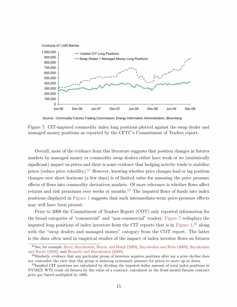
Figure 7: CIT-imputed commodity index long positions plotted against the swap dealer andmanaged money positions as reported by the CFTC’s Commitment of Traders report.
Overall, most of the evidence from this literature suggests that position changes in futures
markets by managed money or commodity swap dealers either have weak or no (statistically
significant) impact on prices and there is some evidence that hedging activity tends to stabilize
prices (reduce price volatility).21 However, knowing whether price changes lead or lag position
changes over short horizons (a few days) is of limited value for assessing the price pressure
effects of flows into commodity derivatives markets. Of more relevance is whether flows affect
returns and risk premiums over weeks or months.22 The imputed flows of funds into index
positions displayed in Figure 1 suggests that such intermediate-term price-pressure effects
may well have been present.
Prior to 2009 the Commitment of Traders Report (COT) only reported information for
the broad categories of “commercial” and “non-commercial” traders. Figure 7 redisplays the
imputed long positions of index investors from the CIT reports that is in Figure 1,23 along
with the “swap dealers and managed money” category from the COT report. The latter
is the data often used in empirical studies of the impact of index investor flows on futures
21See, for example, Boyd, Buyuksahin, Harris, and Haigh (2009), Buyuksahin and Robe (2009), Buyuksahinand Harris (2009), and Brunetti and Buyuksahin (2009).
22Similarly, evidence that any particular group of investors acquires positions after say a price decline doesnot contradict the view that this group is inducing systematic pressure for prices to move up or down.
23Implied CIT positions are calculated by dividing the imputed dollar amount of total index positions inNYMEX WTI crude oil futures by the value of a contract, calculated as the front-month futures contractprice per barrel multiplied by 1000.
15
prices. Clearly these two series are very different, particularly from the fourth quarter of 2007
through the third quarter of 2008, and then again through the second half of 2009. This
graph lends support to the view that the CFTC’s COT data does not give a reliable picture
of the overall demand for and supply of commodity risk exposure.
Perhaps the most compelling evidence to date that index flows and “limits to arbitrage”
have, together, had economically important effects on futures prices is provided by Mou
(2010)’s analysis of excess returns around the dates of the rolls of the futures positions in the
GSCI index. He argues that speculators made substantial profits effectively at the expense of
index investors, particularly for energy-related contracts. Moreover, the profitability of the
trading strategies Mou examines were decreasing in the amount of arbitrage capital deployed
in the futures markets and increasing in the proportion of futures positions attributable to
index fund investments.24
4.2 New Evidence on the Impact of Trader Flows on Oil Prices
In the light of this conflicting evidence on the impact of trader positions on futures prices,
I explore complementary statistical relationships using the imputed flows by index and
managed-money investors. Specifically, I compute weekly time-series of excess returns from
holding positions in futures at different maturity points along the yield curve. The maturities
are the 1, 3, 6, 9, 12, 15, 18, 24, and 36 month contracts, and the sample period is September
12, 2006 through January 12, 2010. Details of the excess return calculations are presented in
the Appendix.
I include the following list of predictor variables for excess returns, with n set to one week
or four weeks, depending on the holding period of the futures position:
RSPn and REMn : the n-week returns on the S&P500 and the MSCI Emerging Asia
indices, respectively. Inclusion of these returns controls for the possibility that investors were
pursuing trading strategies in oil futures that conditioned on recent developments in global
equity markets.
REPOn : the n-week change in overnight repo positions on Treasury bonds by primary
dealers. Etula (2010) in the context of futures trading, and Adrian, Moench, and Shin (2010)
more generally, argue that the balance sheets of financial institutions affect their willingness
to commit capital to risky investments. This in turn implies that risk premiums may depend
on the costs to these institutions of financing their trading activities. The growth in overnight
repo positions is one indicator of balance-sheet flexibility.
24While the profitability of such positions declined leading up to the boom of 2008, they remained positivesuggesting that there were limits to the amount of speculative capital investors were willing to deploy.
16

IIP13 : the thirteen-week change in the imputed positions of index investors in millions,
computed using the same algorithm as in Masters (2009). In contrast to most of the extant
literature, I focus on changes in index positions measured over three months (thirteen weeks)
rather than over a few days or a week.25
MMSPD13 : the thirteen-week change in managed-money spread positions in millions, as
constructed by the CFTC. Erb and Harvey (2006) and Fuertes, Miffre, and Rallis (2008)
document that simple spread trades based on the term structure of futures prices led to
large historical returns. Buyuksahin and Robe (2011) argue that increased positions of hedge
funds in commodity futures affected the correlations correlations between energy futures
and returns on the S&P500 index, and thereby the distribution of oil futures prices. Spread
positions were the largest component of open interest during my sample period (Buyuksahin,
Haigh, Harris, Overdahl, and Robe (2008)), and the disaggregated COT reports show that
managed money accounts showed substantial growth in spread positions. Spread trades are
not signed: trades that are long or short the long-dated futures are treated symmetrically.
OI13 : the thirteen-week change in aggregate open interest in millions, as constructed by the
CFTC. Hong and Yogo (2010) find that increases in open interest over an annual window
predict monthly excess returns on futures. One explanation for this finding is that investors
are learning about fundamental macroeconomic information from both past prices and open
interest. I account for this potential effect by conditioning on the three-month change in
aggregate open interest in oil futures.
AVBASn : the n-week change in average basis. Defining the basis at time t of a futures
contract with maturity Ti(t) to be26
Bi(t) =
(F Tit
St
)1/(Ti(t)−t)
− 1, (7)
as in Hong and Yogo (2010), then AVBAS1 is the average of these values for maturities
i ∈ {1, 3, 6, 9, 12, 15, 18, 21, 24}. In computing (7) I account for the time-varying maturity of
the futures contracts. Hong and Yogo condition on their measure of basis to capture possible
25The flows computed using the methodology in Masters (2009) is not without its limitations. However,for analyzing forecasts of changes in futures prices, it is not necessary that IIP13 be a perfect measure ofthe flow of funds into index positions. Some measurement errors seem inevitable. If the proportion of eachindex made up of any one agricultural product is small, mismeasurement is likely to be amplified through thescaling process. Further, valuation is done at the near-contract futures price (as was the case in Tang andXiong (2011)), and this might not have been how index traders positioned the actual fund flows in oil markets.Supporting this construction, the evidence in Buyuksahin, Haigh, Harris, Overdahl, and Robe (2008), basedon proprietary CFTC data, suggests that the net positions of commodity swap dealers were primarily inshort-dated futures contracts (three months or under).
26Note that this measure of the basis has the opposite sign of the basis in Figure 4.
17

effects of hedging pressures on subsequent returns on futures positions.27
Of equal interest is that AV BASn is a proxy for the net convenience yield in commodity
markets. Recall from (5) that expected excess returns in commodity markets are in general
influenced by variation in convenience yields, changes in market risk premiums, and factors
related to agents’ learning from market prices or forecasting the forecasts of others. To
the extent that AV BASn is a reasonable proxy for the convenience yield in oil markets,
conditioning on AV BASn allows me to highlight the effects of other conditioning variables
on risk premiums or other factors related to limits to arbitrage or speculative behavior.28
Finally, I condition on the lagged value of the realized n-week excess return on oil futures
positions. Stoll and Whaley (2009) find that, once lagged returns on futures positions
are included in predictive regressions, there is no incremental predictive power for flows
into commodity index investment. However, for a much broader set of commodities, Hong
and Yogo (2010) find a very strong predictive relationship between current open interest
and subsequent returns on futures positions, with open interest effectively driving out the
forecasting power of lagged returns.
I estimated the forecasting equations
ERmMt+n(n) = µnm + ΠnmXt + ΨnmERmMt(n) + εm,t+n(n), (8)
where ERmMt(n) is the realized excess return for an n-week investment horizon on a futures
position that expires in m months, Xt is the set of predictor variables, and the data were
sampled at weekly intervals. The fitted values from these regressions are typically interpreted
as expected excess returns in futures markets. This is a natural interpretation when Xt
represents information that was readily available to at least some market participants at the
time the forecasts were formed. The variables IIP13 and MMSPD13 were constructed (by
the CFTC) based on information at the time of the forecast. However this data was released
by the CFTC starting in 2009 and, as such, was not readily available to market participants
27There is an extensive literature examining links between net positions of hedgers and the forecastabilityof commodity returns– the “hedging pressure” hypothesis (Keynes (1930), Hicks (1939)). In two recentexplorations of this issue Gorton, Hayashi, and Rouwenhorst (2007) find no support for the hedging pressurehypothesis, while Basu and Miffre (2010) argue that systematic hedging pressure is an important determinantof risk premiums. Both use the aggregated CFTC data on commercial and non-commercial traders in futuresmarkets, a very course categorization that, as can be seen from Figure 7, is not reliably informative aboutthe trading activities of such classes of investors as index investors or hedge funds.
28Gorton, Hayashi, and Rouwenhorst (2007) extend the model of Deaton and Laroque (1996) to allowfor risk averse speculators (maintaining mean reverting demand) and show that inventories are negativelyrelated to expected excess returns in futures markets. They also establish a link between the futures basisand inventories. These authors and Hong and Yogo (2010), among others, present empirical evidence that ahigh basis (high M2−M4 in Figure 4) predicts high excess returns on futures positions, consistent with thetheory of normal backwardation and compatible with the theory of storage.
18

Variable RSP1 REM1 REPO1 IIP13 MMSPD13 OI13 AVBAS1Contemporaneous Predictors
ER1M(1) 0.35 0.40 0.10 0.21 0.16 0.12 -0.43ER3M(1) 0.43 0.48 0.08 0.24 0.19 0.15 -0.26ER6M(1) 0.45 0.50 0.06 0.25 0.17 0.15 -0.21ER12M(1) 0.44 0.51 0.04 0.25 0.15 0.14 -0.17ER24M(1) 0.41 0.48 0.04 0.25 0.12 0.13 -0.12
Lagged PredictorsER1M(1) 0.03 -0.17 -0.21 0.25 0.18 0.12 -0.25ER3M(1) 0.11 -0.10 -0.20 0.26 0.19 0.13 -0.32ER6M(1) 0.13 -0.09 -0.19 0.26 0.18 0.13 -0.30ER12M(1) 0.16 -0.10 -0.19 0.26 0.16 0.12 -0.24ER24M(1) 0.15 -0.11 -0.17 0.25 0.13 0.11 -0.18
Table 1: Correlations among the one-week excess returns on futures positions and thecontemporaneous and lagged values of the predictor variables.
during my sample period. Therefore, a finding of economically important effects of these
variables on ERmMt+n(n) represents evidence of price pressure effects of flows by these
investor classes on futures prices (controlling for other variables in Xt), but not necessarily
evidence that investors conditioned on these variables in forecasting future oil prices.
The correlations among the ERmM(1) and both contemporaneous and first-lagged values
of the conditioning variables X are displayed in Table 1. The contemporaneous correlations
between the excess returns and the predictor variables have signs that are consistent with
previous findings in the literature. The correlations of the excess returns with emerging
market stock returns (REM1) and the growth in repo positions by primary dealers (REPO1)
change sign when these conditioning variables are lagged one period. Moreover, when investor
flows are measured over periods of weeks, rather than days as in much of the literature, they
have sizable correlations with excess returns. I elaborate on these findings below.
The correlations between changes in oil futures prices and both index and managed-
money flows are positive. For the signed index positions, this is consistent with positive
(momentum-type) price pressure effects. Notice also that the thirteen-week change in open
interest is positively correlated with oil price changes. This finding is consistent with the
strong positive correlation of these variables found by Hong and Yogo (2010) using monthly
data over a much longer sample period. They interpret these correlations as indicative of
open interest embodying information about future economic activity that investors find useful
for predicting future commodity prices. Such a role of open interest would naturally arise in
economic environments where investors learn from past prices and trading volumes as in the
19

models discussed in Section 2. Supporting such an informational role, Hong and Yogo also
find that open interest has predictive content for bond returns and inflation in the U.S.
To explore these comovements more systematically and jointly, I estimated the parameters
in (8) using linear least-squares projection. The null hypotheses are that the elements
of Π are zero: excess returns on futures positions are not predictable by the variables
in Xt, after conditioning on lagged information about excess returns. Economic theory
allows for the possibility that other transformations of the conditioning information (more
lags or nonlinear transformations) have incremental predictive content for excess returns.
Accordingly, following Hansen (1982) and Hansen and Singleton (1982), robust standard
errors are computed allowing for serial correlation and conditional heteroskedasticity in εt+n.29
Estimates of Π along with their asymptotic “t-statistics” are displayed in Tables 2 and 3 for
n = 1 and 4, respectively.
In interpreting these results, it is useful to bear in mind that, assuming that futures
returns and the predictor variables are covariance stationary, the null hypothesis that the
coefficient on investor flows in projections of weekly returns on intermediate-term growth rates
in investor flows has the same economic content as the null hypothesis that short-term flows
impact futures prices over intermediate-term horizons (Hodrick (1992), Singleton (2006)).
Consistent with most prior studies, including weekly changes in index positions has little
predictive content for the weekly excess returns. These observations suggest that, if present,
the price drift in futures markets related to learning and speculative trade is manifested
over return horizons of a few weeks or months. Correlations between futures prices and flow
variables sampled at high frequency are likely to be dominated by noise that obscures the
presence of this longer-horizon comovement.
The adjusted R2’s in these projections provide compelling evidence that excess returns on
futures positions in oil markets had a significant predictable component during this sample
period. From Figure 8 it is seen that the volatilities of the one-week excess returns decline,
and the mean excess returns are increasing, in the contract month. Thus, the low adjusted
R2’s for the longer maturity contracts in Table 2 imply that the predictor variables explain
smaller percentages of relatively less volatile, but larger on average, returns.
Consider first the coefficients on the growth in open interest (OI13). Interestingly, for the
case of n = 1, the coefficients on OI13 (partial correlations) switch sign and shrink in absolute
value relative to the correlations in Table 1, and they are small relative to their estimated
standard errors. After conditioning on the trading patterns of index investors and hedge
funds, at least for the sample period around the 2008 boom/bust, open interest does not have
significant predictive content for one-week excess returns. Nevertheless, market participants
29Specifically, I use the Newey and West (1987) construction allowing for five lags.
20

Con
trac
tR
SP
1R
EM
1R
EP
O1
IIP
13M
MSP
D13
OI1
3A
VB
AS1
RLag
AdjR
2
10.
332
-0.3
42-0
.201
0.27
20.
357
-0.1
03-4
.165
-0.2
190.
27(1
.44)
(-2.
44)
(-2.
89)
(3.5
1)(4
.36)
(-2.
17)
(-6.
26)
(-2.
05)
30.
361
-0.2
42-0
.170
0.21
80.
284
-0.0
82-3
.661
-0.1
520.
27(1
.99)
(-2.
02)
(-2.
76)
(3.7
1)(4
.43)
(-1.
87)
(-6.
48)
(-2.
10)
60.
391
-0.2
61-0
.150
0.19
70.
245
-0.0
72-3
.022
-0.1
050.
25(2
.35)
(-2.
27)
(-2.
64)
(3.4
9)(4
.14)
(-1.
74)
(-5.
59)
(-1.
62)
90.
424
-0.2
75-0
.142
0.18
70.
222
-0.0
67-2
.551
-0.0
900.
24(2
.67)
(-2.
46)
(-2.
58)
(3.4
5)(3
.95)
(-1.
73)
(-4.
72)
(-1.
40)
120.
437
-0.2
83-0
.133
0.17
90.
202
-0.0
64-2
.141
-0.0
750.
22(2
.84)
(-2.
60)
(-2.
49)
(3.4
2)(3
.83)
(-1.
73)
(-3.
97)
(-1.
14)
180.
430
-0.2
86-0
.119
0.16
60.
174
-0.0
58-1
.657
-0.0
540.
20(2
.99)
(-2.
79)
(-2.
35)
(3.4
2)(3
.61)
(-1.
72)
(-3.
13)
(-0.
75)
240.
412
-0.2
87-0
.107
0.15
70.
159
-0.0
53-1
.329
-0.0
460.
18(2
.98)
(-2.
87)
(-2.
21)
(3.4
6)(3
.40)
(-1.
67)
(-2.
60)
(-0.
59)
360.
378
-0.2
94-0
.093
0.14
50.
144
-0.0
48-0
.981
-0.0
330.
16(2
.85)
(-2.
99)
(-2.
05)
(3.5
2)(3
.02)
(-1.
60)
(-2.
10)
(-0.
40)
Tab
le2:
Est
imat
esan
dro
bust
test
stat
isti
csfo
rth
efu
ture
sex
cess
retu
rnfo
reca
stin
gm
odel
over
the
hor
izon
ofon
ew
eek
(ERmM
(1)
isth
edep
enden
tva
riab
le).
21

Con
trac
tR
SP
4R
EM
4R
EP
O4
IIP
13M
MSP
D13
OI1
3A
VB
AS4
RLag
AdjR
2
10.
023
0.24
60.
097
0.98
70.
972
-0.4
47-1
.33
-0.2
290.
38(.
061)
(1.2
2)(1
.39)
(4.3
6)(6
.95)
(-3.
91)
(-.6
88)
(-2.
04)
3-0
.137
0.34
20.
038
0.92
70.
934
-0.3
740.
121
-0.2
790.
41(-
.521
)(2
.36)
(.56
4)(4
.54)
(7.0
3)(-
3.36
)(.
095)
(-2.
59)
6-0
.200
0.35
10.
015
0.88
00.
833
-0.3
380.
539
-0.2
710.
39(-
.783
)(2
.58)
(.23
7)(4
.32)
(6.7
1)(-
3.22
)(.
452)
(-2.
33)
9-0
.216
0.33
00.
015
0.84
60.
756
-0.3
220.
707
-0.2
540.
37(-
.854
)(2
.52)
(.24
8)(4
.30)
(6.4
0)(-
3.21
)(.
611)
(-2.
10)
12-0
.222
0.31
20.
017
0.81
10.
689
-0.3
060.
782
-0.2
380.
36(-
.886
)(2
.48)
(.29
5)(4
.25)
(6.1
1)(-
3.14
)(.
693)
(-1.
92)
18-0
.219
0.27
60.
023
0.74
40.
588
-0.2
780.
776
-0.2
110.
33(-
.902
)(2
.36)
(.43
2)(4
.20)
(5.6
0)(-
2.97
)(.
726)
(-1.
68)
24-0
.213
0.25
00.
029
0.68
70.
531
-0.2
550.
706
-0.1
900.
31(-
.915
)(2
.30)
(.57
1)(4
.15)
(5.3
4)(-
2.83
)(.
701)
(-1.
49)
36-0
.212
0.23
70.
036
0.61
30.
480
-0.2
360.
412
-0.1
750.
28(-
.993
)(2
.43)
(.78
7)(4
.06)
(4.9
5)(-
2.78
)(.
454)
(-1.
37)
Tab
le3:
Est
imat
esan
dro
bust
test
stat
isti
csfo
rth
efu
ture
sex
cess
retu
rnfo
reca
stin
gm
odel
over
the
hor
izon
offo
ur
wee
ks
(ERmM
(4)
isth
edep
enden
tva
riab
le).
22

0 10 20 30 40 50 60−10
−5
0
5
10
15
20
25
Contract month
mean 1W rolling return (in bp)
(a) Sample Mean
0 10 20 30 40 50 603.5
4
4.5
5
5.5
6
6.5Std Dev 1W rolling return (in %)
Contract month
(b) Sample Standard Deviation
Figure 8: Sample moments in basis points of the weekly excess returns on futures.
who did not observe the information about investor flows summarized by (IIP13,MMSPD13)
may well have found it informative to condition on order-flow information when estimating
risk premiums in futures markets. The sample correlation between IIP13 (MMSPD13) and
OI13 was 0.56 (0.45).
Interestingly, OI13 has a statistically significant negative effect on the four-week excess
returns ERmM(4) (Table 3) for all contract maturities. This negative effect, which declines
monotonically with the maturities of the futures contracts, is the opposite of the finding
in Hong and Yogo (2010). However, they did not condition on the investor flows IIP13 or
MMSPD13 and the negative coefficients may well reflect interactions in the ways these
three variables are informative about monthly holding period returns in futures markets.
Perhaps the most striking findings in Tables 2 and 3 are the statistically significant
predictive powers of changes in the index investor (IIP13) and managed money spread
(MMSPD13) positions on excess returns in crude oil futures markets. Increases in flows
into index funds over the preceding three months predict higher subsequent futures prices.
These effects are significant for contracts of all maturities, after controlling for lagged futures
returns and the other conditioning variables in Xt. The flow variable IIP13 is capturing price
pressures associated with intermediate-term persistent flows of funds into index positions.
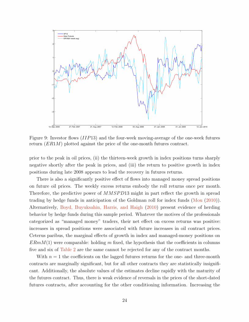
The significant positive relationship between futures excess returns and index investor
flows is seen visually from a comparison of IIP13, the four-week moving average of ER1M(1),
and the price of the one-month futures contract (Figure 9).30 Other notable features of this
figure are: (i) both the futures returns and IIP13 start to decline in the spring of 2008
30This series is the price of the generic one-month futures contract, CL1, from Bloomberg.
23
12−Sep−2006 27−Feb−2007 21−Aug−2007 12−Feb−2008 05−Aug−2008 27−Jan−2009 21−Jul−2009 12−Jan−2010−4
−3
−2
−1
0
1
2
3
IIP13Near FuturesER1M(4−week avg)
Figure 9: Investor flows (IIP13) and the four-week moving-average of the one-week futuresreturn (ER1M) plotted against the price of the one-month futures contract.
prior to the peak in oil prices, (ii) the thirteen-week growth in index positions turns sharply
negative shortly after the peak in prices, and (iii) the return to positive growth in index
positions during late 2008 appears to lead the recovery in futures returns.
There is also a significantly positive effect of flows into managed money spread positions
on future oil prices. The weekly excess returns embody the roll returns once per month.
Therefore, the predictive power of MMSPD13 might in part reflect the growth in spread
trading by hedge funds in anticipation of the Goldman roll for index funds (Mou (2010)).
Alternatively, Boyd, Buyuksahin, Harris, and Haigh (2010) present evidence of herding
behavior by hedge funds during this sample period. Whatever the motives of the professionals
categorized as “managed money” traders, their net effect on excess returns was positive:
increases in spread positions were associated with future increases in oil contract prices.
Ceterus paribus, the marginal effects of growth in index and managed-money positions on
ERmM(1) were comparable: holding m fixed, the hypothesis that the coefficients in columns
five and six of Table 2 are the same cannot be rejected for any of the contract months.
With n = 1 the coefficients on the lagged futures returns for the one- and three-month
contracts are marginally significant, but for all other contracts they are statistically insignifi-
cant. Additionally, the absolute values of the estimates decline rapidly with the maturity of
the futures contract. Thus, there is weak evidence of reversals in the prices of the short-dated
futures contracts, after accounting for the other conditioning information. Increasing the
24

holding period to n = 4 weeks does not alter the signs of these coefficients, though they
remain statistically significant for contracts out to about one year in length.
More generally, and importantly for interpreting the evidence regarding the boom and bust
in oil prices, these findings suggest that the significant predictive content of the conditioning
variables Xt is fully robust to inclusion of the lagged return (see also below). This stands in
contrast to the results from focusing on returns and conditioning variables over daily intervals
as, for instance, in Buyuksahin and Harris (2009) and Stoll and Whaley (2009).
The coefficients in Table 2 on the lagged returns on emerging market equity positions
(REM1) are negative and statistically significant. In contrast, the signs on the coefficients
on REM4 in the projections for four-week excess returns ERmM(4) are positive, as are the
contemporaneous correlations between the ERmM(1) and REM1. To explore this change of
sign in more depth, I project ERmMt+j(1) onto Xt (for the case of n = 1) and ERmM(1)t,
for j = 1, 2, 3, 4. The coefficients on REM1t in these projections effectively trace out the
conditional impulse response function of ERmM(1) to an innovation in REM1. They start
negative, turn positive in week two and peak at a larger positive number at week three. This
pattern suggests that, after controlling for the other variables in Xt, positive innovations
in (favorable news about) emerging market growth predicted reversals in futures prices in
the subsequent week, perhaps as a consequence of limits to capital market intermediation or
learning mechanisms that lead to short-term over-shooting of prices. Then, over somewhat
longer horizons, such news predicts positive futures returns.
The negative and statistically significant effects of REPO1 on excess returns are consistent
with the model of Etula (2010) in which risk limits and funding pressures faced by broker-
dealers impact risk premiums in commodity markets. The OTC commodity derivatives
market is substantially larger than the markets for exchange traded products and servicing
the OTC markets requires a substantial commitment of capital by broker-dealers. As funding
conditions improve– reflected here through an increase in the repo positions of primary dealers–
the effective risk aversion of broker-dealers declines and, hence, so should the expected excess
returns in commodity futures markets. This effect of funding liquidity on excess returns
declines (in absolute value) with contract maturity, while remaining statistically significant.
Moreover, the statistically insignificant effects on ERmM(4) in Table 3 indicate that any
partial effects of funding liquidity where short-lived after conditioning on trader positions.
Finally, increases in the average basis (AV BAS1) are associated with declines in excess
returns. The coefficients on AV BAS1 are both more negative and statistically significant for
the short-maturity contracts. AV BAS1 shows small bilateral correlations with the other con-
ditioning variables. For instance, its correlations with (REPO1, IIP13,MMSPD13, OI13)
are (−0.15,−0.05,−0.05,−0.08) so the weekly average basis represents distinct information
25

about future returns. Over monthly horizons the effect of AV BAS4 is not statistically
significant. This finding aligns with those in studies of earlier sample periods (e.g., Fama
and French (1987)), and also to those in Hong and Yogo (2010) who examine monthly excess
returns over the longer sample period 1987-2008.
As noted previously, AV BAS1 is a proxy for the convenience yield on oil markets. Some
insight into whether my results are documenting the effects of risk premiums and expectational
errors or convenience yields on excess returns can be gleaned from examining the errors from
forecasting future spots prices using futures prices. Toward this end I projected St+4 − F t+4t
(the spot price one month ahead minus the one-month futures price) onto the conditioning
variables Xt (for the monthly horizon).31 The adjusted R2 in this projection is 0.39, similar to
the result for ER1M in Table 3. Only the investor flow variables IIP13 and MMSPD13 enter
with statistically significant coefficients. That these flow variables have predictive content
suggests that they are impacting commodity prices through risk premiums or speculative
expectational terms, consistent with the conceptual frameworks outlined above. Of equal
interest is the finding that neither OI13 nor REM4 enter significantly. It seems that, for this
horizon, traders’ reactions to news about emerging market equity returns and open interest
helped shaped the futures curve, but not so much spot market risk premiums.
The reported findings are robust to inclusion of several other conditioning variables. In
preliminary regressions I also included the one-week change in the Cushing, OK inventory
of crude oil in millions, as reported on Bloomberg, to check the robustness of the results
to the inclusion of inventory information. There is a statistically weak negative effect of
inventory information on the excess return for the one-month contract. Beyond one month
the coefficients are all small relative to their estimated standard errors.
Additionally, I estimated the predictive regressions with additional lags of excess returns
included as predictor variables and the pattern of results in Table 2 remained qualitatively
the same. The inclusion of past information about returns does not materially affect the
predictive content of the investor flow variables.
Finally, some argue that the trading patterns of index and managed-money investors are
linked to speculation about global economic growth. A relevant question then is whether
measures of global economic growth also had predictive power for excess returns on futures.
As a proxy for aggregate demand, I follow Kilian (2009) and Pirrong (2009), as well as
many oil-market practitioners, and use shipping rates based on the Baltic Exchange Dry
Index (BEDI). The growth rate of the BEDI over the previous three months does explain
31Using data on three shortest maturity futures contracts a cubic spline was used to interpolate for theone-month futures price. Two different interpolations schemes were examined and they gave qualitativelyidentical results.
26

an additional 2− 3% of the variation in excess returns, and its coefficients are marginally
statistically significant. However, BEDI has very little effect on the explanatory power of the
other predictors: they continue to explain most of the variation in futures returns.
5 Concluding Remarks
The trading patterns of investors who are learning about economic fundamentals, both from
public announcements and market prices, may contribute to drift in commodity prices that
looks like a boom followed by a bust. This phenomenon is entirely absent, essentially by
assumption, from many of the models of oil price determination that focus on representative
suppliers, consumers, and hedgers. My empirical evidence suggests that growth in positions
of index investors and managed-money accounts had significant positive effects on returns in
oil futures markets around the time 2008 boom/bust in oil prices, after accounting for stock
returns in the U.S. and emerging economies, open interest, and lagged futures returns.
The welfare costs of trading based on imperfect information are potentially amplified by
the fact that the costs to individual investors of near-rational behavior – following slightly
suboptimal investment or consumption plans– is negligible and yet this behavior might be
quite costly for society as a whole (Lucas (1987) and Cochrane (1989)).32 When investors make
small correlated errors around their optimal investment policies, financial markets amplify
these errors and generate price changes that are unrelated to fundamental supply/demand
information (Hassan and Mertens (2010)). If index investors are just slightly too optimistic
(in market rallies) or pessimistic (in market downturns) relative to the true state of the world
then their errors, while inconsequential for their own welfare, may be material for society as
a whole.33 Frictions associated with multi-period contracting over labor and physical capital
will likely exacerbate the social costs of any price drift.
More broadly, it is the dynamic interactions of the trading activities of index investors,
hedge funds, broker/dealers in commodity markets, and commercial hedgers that ultimately
set prices in commodity spot and futures markets. Just as index investors are, in part,
adjusting their positions based on their views about global supplies and demands, other
32Such suboptimal plans may arise out of misinterpretations of public information say about futureeconomic growth in developing countries, because of small costs to sorting through the complexity of globaleconomic developments and their implications for commodity prices, or because of over-confidence aboutfuture economic growth as in Dumas, Kurshev, and Uppal (2006).
33Recent research by Qiu and Wang (2010) shows that when market participants have heterogeneousinformation, and so asset prices depend on the expectations of the expectations of others, prices tend tobe more volatile and the overall welfare of society is lowered. Additionally, if index traders impart noise tomarket prices through their trading activities, then this could also reduce the efficiency with which futuresand spot markets perform their roles in price discovery.
27

market participants are doing likewise and they are positioning based on their views about
what index and other classes of investors are doing. This may well explain the significant
effects of hedge fund spread positions on excess returns in oil markets documented here.
Finally, much of the literature on commodity pricing abstracts from the impact of the
extensive array of derivatives contracts in commodity markets (e.g., commodity swaps)
on market-price dynamics. Adding derivatives markets may improve price discovery and
mitigate some of the informational problems highlighted above. A key step towards a better
understanding of the effects of interactions among various market participants on price
behavior is the collection and dissemination of more detailed information about the trading
patterns in OTC commodity derivatives, as well as exchange traded futures.
28

Appendix: Construction of Excess Returns
Let FTi(t)t denote the futures contract with expiration Ti(t). The futures-price-term-structure
consists of points FT1(t)t , ..., F
TN (t)t . Let D(s) > s denote the first time after s that the generic
futures curve switches contracts. Then, for all i = 1, ..., N − 1, and all s,
Ti+1(D(s)− 1) = Ti(D(s))
The excess rolling return in generic contract i, between s and t is given by
FTi(t)t
FTi(s)s
− 1 if t < D(s)
FTi(D(s)−1)D(s)−1
FTi(s)s
· FTi(t)t
FTi+1(D(s)−1)D(s)−1
− 1 if D(s) ≤ t < D(2)(s)
FTi(D(s)−1)D(s)−1
FTi(s)s
·FTi(D
(2)(s)−1)D(2)(s)−1
FTi+1(D(s)−1)D(s)−1
· FTi(t)t
FTi+1(D(2)(s)−1)D(2)(s)−1
− 1 if D(2)(s) ≤ t < D(3)(s)
and so forth.
By construction these are the net returns from holding one long position in the generic
i-month contract, liquidating the position the day before the generic curve “moves the
contracts one month down,” and going long one unit in the following month i+ 1 (which the
day after, by definition will be generic contract i). This strategy is followed from s until t.
The riskfree rate does not enter these calculations. The rational is (following, for instance,
Etula (2010)) that investing in a futures position, does not require an initial capital injection.
In practice, however, the futures trading strategies are met with margin calls. For this reason
Hong and Yogo (2010) consider a fully collateralized return of the form (say if t < D(s))
FTi(t)t
FTi(s)s
Rfs,t
My calculations omit the multiplying factor Rfs,t from the construction of excess returns.
29

References
Acharya, V., L. Lochstoer, and T. Ramadorai, 2009, “Limits to Arbitrage and Hedging:
Evidence from Commodity Markets,” working paper, New York University.
Adam, K., and A. Marcet, 2010a, “Booms and Busts in Asset Markets,” working paper,
IMES Discussion Paper 2010-E-2, Bank of Japan.
, 2010b, “Internal Rationality, Imperfect Market Knowledge and Asset Prices,” working
paper, forthcoming, Journal of Economic Theory.
Adrian, T., E. Moench, and H. Shin, 2010, “Financial Intermediation, Asset Prices, and
Macroeconomic Dynamics,” working paper, Federal Reserve Bank of New York Staff Report
422.
Aguiar, M., and G. Gopinath, 2007, “Emerging Market Business Cycles: The Cycle is the
Trend,” Journal of Political Economy, 115, 69–102.
Allen, F., S. Morris, and H. Shin, 2006, “Beauty Contests and Iterated Expectations in Asset
Markets,” Review of Financial Studies, 19, 719–752.
Alquist, R., and L. Kilian, 2010, “What Do We Learn From the Price of Crude Oil Futures?,”
Journal of Applied Econometrics, 25, 539–573.
Banerjee, S., R. Kaniel, and I. Kremer, 2009, “Price Drift as an Outcome of DIfferences in
Higher-Order Beliefs,” Review of Financial Studies, 22, 3707–3734.
Banerjee, S., and I. Kremer, 2010, “Disagreement and Learning: Dynamic Patterns of Trade,”
Journal of Finance, LXV, 1269–1302.
Basu, D., and J. Miffre, 2010, “Capturing the Risk Premium of Commodity Futures: The
Role of Hedging Pressure,” working paper.
Boyd, N., B. Buyuksahin, J. Harris, and M. Haigh, 2009, “The Impact of Hedging on Futures
Prices,” working paper, U.S. Commodity Futures Trading Commission.
, 2010, “The Prevelence, Sources and Effects of Herding,” working paper, U.S.
Commodity Futures Trading Commission.
Brunetti, C., and B. Buyuksahin, 2009, “Is Speculation Destabilizing?,” working paper,
Commodity Futures Trading Commission.
30
Buyuksahin, B., M. Haigh, J. Harris, J. Overdahl, and M. Robe, 2008, “Fundamentals, Trader
Activity and Derivative Pricing,” working paper, Commodity Futures Trading Commission.
Buyuksahin, B., and J. Harris, 2009, “The Role of Speculators in the Crude Oil Futures
Market,” working paper, Commodity Futures Trading Commission.
Buyuksahin, B., and M. Robe, 2009, “Commodity Traders’ Positions and Energy Prices:
Evidence from the Recent Boom-Bust Cycle,” working paper, U.S. Commodity Futures
Trading Commission.
, 2010, “Hedge Funds, Stress, and Cross-Market Linkages,” working paper, Commodity
Futures Trading Commission.
, 2011, “Does “Paper Oil” Matter? Energy Markets’ Financialization and Equity-
Commodity Co-Movements,” working paper, International Energy Agency.
Cao, H., and Ou-Yang, 2009, “Differences in Opinion of Public Information and Speculative
Trading in Stocks and Options,” Review of Financial Studies, 22, 299–335.
Casassus, J., and P. Collin-Dufresne, 2005, “Stochastic Convenience Yield Implied from
Commodity Futures and Interest Rates,” Journal of Finance, LX, 2283–2331.
Cochrane, J., 1989, “The Sensitivity of Tests of the Intertemporal Allocation of Consumption
to Near-Rational Alternatives,” American Economic Review, 79, 319–337.
Corkery, M., and C. Cui, 2010, “Calstrs Reins in Plans for a Big Bet,” Wall Street Journal,
November 12, 2010.
Deaton, A., and G. Laroque, 1996, “Competitive Storage and Commodity Price Dynamics,”
Journal of Political Economy, 104, 896–923.
Dumas, B., A. Kurshev, and R. Uppal, 2006, “What Can Rational Investors Do About
Excessive Volatility and Sentiment Fluctuations?,” working paper, Swiss Finance Institute
Research Paper No. 06-19.
Dvir, E., and K. Rogoff, 2009, “The Three Epochs of Oil,” working paper, Harvard University.
Erb, C., and C. Harvey, 2006, “The Strategic and Tactical Value of Commodity Futures,”
Financial Analysts Journal, 62, 69–97.
Etula, E., 2010, “Broker-Dealer Risk Appetite and Commodity Returns,” working paper,
Federal Reserve Bank of New York.
31

Evans, M., and R. Lyons, 2009, “Forecasting Exchange Rate Fundamentals with Order Flow,”
working paper, University of California, Berkeley.
Fama, E., and K. French, 1987, “Commodity Futures Prices: Some Evidence on Forecast
Power, Premiums, and the Theory of Storage,” Journal of Business, 60, 55–73.
Fuertes, A., J. Miffre, and G. Rallis, 2008, “Tactical Allocation in Commodity Futures
Markets: Combining Momentum and Term Structure Signals,” working paper, EDHEC.
Gorton, G., F. Hayashi, and K. Rouwenhorst, 2007, “The Fundamentals of Commodity
Futures Returns,” working paper, Yale University.
Hamilton, J., 2003, “What is An Oil Shock?,” Journal of Econometrics, 113, 363–398.
, 2009a, “Causes and Consequences of the Oil Shock of 2007-08,” Brookings Papers
on Economic Activity.
, 2009b, “Understanding Crude Oil Prices,” Energy Journal, 30, 179–206.
Hansen, L., 1982, “Large Sample Properties of Generalized Method of Moments Estimators,”
Econometrica, 50, 1029–1054.
Hansen, L., and K. Singleton, 1982, “Generalized Instrumental Variables Estimation of
Nonlinear Rational Expectations Models,” Econometrica, 50, 1269–1286.
Hassan, T., and T. Mertens, 2010, “The Social Cost of Near-Rational Investment: Why we
Should Worry about Volatile Stock Markets,” working paper, University of Chicago.
Hicks, J., 1939, Value and Capital. Oxford University Press.
Hodrick, R., 1992, “Dividend Yields and Expected Stock Returns: Alternative Procedures
for Inference and Measurement,” Review of Financial Studies, 5, 357–386.
Hong, H., and M. Yogo, 2010, “Commodity Market Interest and Asset Return Predictability,”
working paper, Princeton University.
Hooker, M., 1996, “What Happened to the Oil Price-Macroeconomy Relationship?,” Journal
of Monetary Economics, 38, 195–213.
IEA, 2008a, “Medium-Term Oil Market Report,” October, International Energy Agency.
, 2008b, “Medium-Term Oil Market Report,” July, International Energy Agency.
32

, 2009, “Oil Market Report,” December, International Energy Agency.
Irwin, S., and D. Sanders, 2010, “The Impact of Index Swap Funds on Commodity Futures
Markets,” working paper, OECD Food, Agriculture and Fisheries Working Papers No. 27.
Keynes, J., 1930, Treatise on Money. Macmillan, London.
Kilian, L., 2009, “Not All Oil Price Shocks Are Alike: Disentangling Demand and Supply
Shocks in the Crude Oil Market,” American Economic Review, 99, 1053–1069.
Lucas, R., 1987, Models of Business Cycles. Basil Blackwell.
Masters, M., 2009, “Testimony Before the Commodity Futures Trading Commission,” working
paper, Commodity Futures Trading Commission.
Milgrom, P., and N. Stokey, 1982, “Information, Trade, and Common Knowledge,” Journal
of Economic Theory, 26, 11–21.
Miltersen, K., and E. Schwartz, 1998, “Pricing of Options on Commodity Futures with
Stochastic Term Structures of Convenience Yields and Interest Rates,” Journal of Financial
and Quantitative Analysis, 33, 33 –59.
Mou, Y., 2010, “Limits to Arbitrage and Commodity Index Investments: Front-Running the
Goldman Roll,” working paper, Columbia Business School.
Newey, W., and K. D. West, 1987, “Hypothesis Testing with Efficient Method of Moment
Estimation,” International Economic Review, 28, 777–787.
Nimark, K., 2009, “Speculative Dynamics in the Term Structure of Interest rates,” working
paper, Universitat Pompeu Fabra.
Pirrong, C., 2009, “Stochastic Fundamental Volatility, Speculation, and Commodity Storage,”
working paper, University of Houston.
Qiu, W., and J. Wang, 2010, “Asset Pricing Under Heterogeneous Information,” working
paper, MIT.
Rotemberg, J., and M. Woodford, 1996, “Imperfect Competition and the Effects of Energy
Price Increases on Economic Activity,” Journal of Money, Credit, and Banking, 28, 550–577.
Saporta, V., M. Trott, and M. Tudela, 2009, “What Can Be Said About the Rise and Fall in
Oil Prices?,” Bank of England Quarterly Bulletin, 49, 215–225.
33

Sauter, R., and S. Awerbuch, 2003, “Oil Price Volatility and Economic Activity: A Survey
and Literature Review,” working paper, IEA Research Paper.
Singleton, K., 1987, “Asset Prices in a Time Series Model with Disparately Informed,
Competitive Traders,” in New Approaches to Monetary Economics, ed. by W. Burnett,
and K. Singleton. Cambridge University Press.
, 2006, Empirical Dynamic Asset Pricing. Princeton University Press.
Sornette, D., R. Woodard, and W. Zhou, 2008, “The 2006-2008 Oil Bubble and Beyond,”
working paper, ETH Zurich.
Stoll, H., and R. Whaley, 2009, “Commodity Index Investing and Commodity Futures Prices,”
working paper, Vanderbilt University.
Tang, K., and W. Xiong, 2011, “Index Investing and the Financialization of Commodities,”
working paper, Princeton University.
Tirole, J., 1982, “On the Possibility of Speculation under Rational Expectations,” Economet-
rica, 50, 1163–1181.
Townsend, R., 1983, “Forecasting the Forecasts of Others,” Journal of Political Economy, 91,
546–588.
Verardo, M., 2009, “Heterogeneous Beliefs and Momentum Profits,” Journal of Financial
and Quantitative Analysis, 44, 795–822.
Verleger, P., 2010, “Comments on Federal Speculative Position Limits for Referenced Energy
Contracts and Associated Regulations,” Federal Register 4144.
Xiong, W., and H. Yan, 2010, “Heterogeneous Expectations and Bond Markets,” Review of
Financial Studies, 23, 1433–1466.
Zhang, F., 2006, “Information Uncertainty and Stock Returns,” Journal of Finance, LXI,
105–36.
34