Investment, Interest Rates, and the Effects of ... · The more sensitive the ... the alternative...

ROBERT E. HALL

Massachusetts Institute of Technology

Investment, Interest Rates,

and the Efects

of Stabilization olicies

THE RESPONSE of investment expenditure to changes in interest rates is at the heart of any analysis of stabilization policy. The more sensitive the response, the more potent is monetary policy and the weaker is fiscal expenditure policy. The stimulus of lower interest rates on investment is one of the principal channels of monetary influence in virtually all macroeconomic theories. On the other hand, the negative influence of higher interest rates on investment may inhibit the macroeconomic effect of expenditure policy. The net effect of government expenditures on gross national product has been and remains the single most important source of disagreement over stabilization policy among economists. My purpose here is to examine the empirical evidence on the interest response of investment with the hope of narrowing the disagreement about the effects of expenditure and monetary policies. Though the evidence is disappointingly weak, it does suggest that the modem Keynesian view embodied in large-scale macroeconometric models-that the expenditure multiplier is around 1.5 -and the simple monetarist view-that it is essentially zero-are both incorrect. The most reasonable value lies in the middle, perhaps at 0.7. Unfortunately, the evidence is probably not strong enough to convince the firm adherent of the other two positions.

Note: This research was supported by the National Science Foundation. I am grateful to Dale W. Jorgenson and members of the Brookings panel for helpful comments.

61

62 Brookings Papers on Economic Activity, 1:1977

The Empirical Issues

The interest response of investment depends fundamentally on the substitutability of capital for other factors, and there seems to be general agreement today that factor substitution can take place. In fact, the uni- tary-elasticity property of the Cobb-Douglas production function is not a bad summary of the findinigs of more general studies: a decline of 1 percent in the service price of capital raises the capital-output ratio by about 1 percent. But this is a long-run relationship, and it is much less generally agreed that the flow that brings about the change in the capital intensity- extra investment-is highly responsive to changes in the price of capital over the one- to three-year horizon of chief concern in stabilization. Skeptics about the interest elasticity of investment point to three considerations that cause the adjustment in factor intensities to take place slowly:

1. Lags in putting capital goods in place. It can take at least a year to design, order, build, and install capital equipment after a change in relative factor prices makes new equipment desirable.

2. The putty-clay hypothesis. Capital already in place cannot be adapted to a different capital intensity; factor proportions are fixed at the time the equipment is designed. Changes in factor intensities dictated by changes in the price of capital take place only as the old capital is replaced.

3. The term structure of interest rates. Stabilization policies affect the short-term interest rate, but investment responds to the long-term rate. Long rates respond to short rates with an important lag.

Evidence from a variety of sources, discussed below, seems to converge on the point that lags in the investment process are long enough to limit the immediate effect of changes in the service price of capital on investment. The investment taking place in a given year is largely the consequence of irrevocable decisions made in earlier years, and only a small fraction can be affected by changes in that year in the financial attractiveness of investment. This consideration makes expenditure policy stronger and monetary policy weaker than they would be in an economy with more flexibility about investment in the short run.

Evidence on the putty-clay hypothesis is much more ambiguous. The paper contains a theoretical exposition of the hypothesis that emphasizes the central issue with respect to its implications for investment behavior:

Robert E. Hall 63

Under putty-clay, firms do not face an economic decision about how much output to produce on their existing capital equipment. If there is such a decision-for example, if more output can be squeezed out of existing equipment by operating it for longer hours or adding more labor in other ways-then the putty-clay hypothesis in its strict form is wrong and the response of investment to the service price of capital is not just the change in the factor intensity of newly installed capacity but involves substitution between new and old capital as well. The paper demonstrates a serious problem in the major existing attempt to measure the influence of the putty-clay phenomenon in the investment equation. No definite conclusion emerges about the importance of putty-clay.

The question of the proper interest rate for an investment equation is tackled only at the theoretical level. The simple argument that capital is long-lived and that consequently the investment decision should be based on the long-term interest rate is examined and confirmed, but this principle does not imply that the service price of capital depends on the long rate. Rather, the service price emerges from a comparison of investment decisions made this year on the basis of this year's long rate, and those that will be made next year on the basis of next year's long rate. This comparison involves the expected change in the long rate, which is measured by the current short rate. As a matter of theory, it seems quite unambiguous that an investment theory built around the concept of a service price of capital should use the short rate. The prospect for empirical confirmation of this principle seems slight, in view of the major difficulties associated with measurement of the role of interest rates of any kind.

An Empirical IS-LM Framework

Generations of economists have been taught to study the effects of monetary and fiscal policy within Hicks' IS-LM framework. In the dia- gram below the IS curve traces the combinations of the interest rate and real gross national product that are consistent with the expenditure side of the economy. Higher interest rates are associated with lower levels of GNP because of the negative response of investment. The LM curve describes the alternative interest rates and levels of GNP that clear the money market. Higher levels of GNP require higher interest rates to clear the market for a given exogenous quantity of money. Increased government

64 Brookings Papers onz Economic Activity, 1:1977

expenditures shift the IS curve to the right, say to IS'. Real GNP rises from Y to Y'. The magnitude of the increase depends on the relative slopes of the two curves: it is large if the LM curve is flat and the IS curve is steep and small in the opposite case. An increased money supply shifts the LM curve to the right, say to LM". Again, the effect on GNP depends on the relative slopes of the two curves: monetary policy is potent if the IS curve is flat and the LM curve is steep.

The central question of this paper can be stated succinctly in the IS-LM framework: how flat is the IS curve relative to the LM curve? An algebraic development of the IS-LM model is a necessary prelude to an empirical study. Start with a simple consumption function:

C - o + 61Y, Interest rate LM LM LM"?

is,

_~~~~ ~ ~~~~~ _ /

f t I 5

y yP ytt ~~~Real GNP

where C is consumption in real terms and Y is real GNP, and thus 0, is the marginal propensity to consume out of GNP. Next is the investment function,

I I+ eY Y-72y;

where I is real investmermt and r is the interest rate; GyN measures the accelerator effect of output on investment and y2 is the crucial interest re-

Robert E. flail 65

sponse. The expenditure side of the economy is governed as well by the GNP identity,

Y = C + I + GI where G is real government expenditures. The IS curve is obtained by solving the three equations for r as a function of Y:

r do + yo + G -(I - 01 - 1) Y 72

The final equation is the money-demand function,

M/p = -1'o + '1 Y - VI2 r,

where M is the nominal money supply and p is the price level; 'P. is the income response of money demand and 2 iS the interest response. The LM curve is just the money-demand function solved for r:

r- 0 + AY - M/p 'P2

The intersection of the IS and LM curves is obtained by equating them and solving for Y:

Y =o + I, G + g2 M/p, where pu, is the effect of expenditures on GNP:

1 1-01 - 7Yl + IP (72/P2)'

Note the crucial role of the ratio of the two slope parameters, y2/'2. If the IS curve is steep and the LM curve is flat, y2/'2 is small and t,u is close to the simple Keynesian multiplier, 1/(1 - 0, - Yl). With a flat IS and a steep LM curve, 72/2 will be large, ,t will be small, and the interest-rate effect will largely offset the simple multiplier effect.

The influence of the real money supply is described by2:

rU= 4 l + (- 01 - 7') (VP2/72)-

Again, the ratio of the slope parameters, 'P2/Y2, plays a central role, now in reciprocal form. If the IS curve is steep and the LM curve is flat, 'P2/y2

is large and pt2 is small. With a flat IS and a steep LM curve, the effect of monetary expansion on GNP will be close to the extreme value of the crude quantity theory, 1/'P,.

How relevant is such a simple model to stabilization policy in the mod-


em U.S. economy? In the first place, it takes the real money supply, M/p, as predetermined by monetary policy. Unless the monetary authorities offset every movement in prices, exogeneity of M/p is realistic only if prices are taken as predetermined-that is, if the price level does not react to developments in the economy within the period.1 This paper is concerned with the effect of stabilization policy only for the first year after policy actions are taken. A good deal of recent research on price determination seems to support unresponsive prices as a reasonable approximation, though there are some important dissenters.

The responsiveness of prices to stabilization policy over a longer horizon influences the results even when the analysis concerns only the initial year after a policy action. Investment depends on the real interest rate while money demand depends on the nominal interest rate, and the difference between them is the expected rate of inflation from one year to the next. The assumption of unresponsive expectations about the rate of inflation could be justified either as an extension of the rigid-price hypothesis to the second year or as a failure of rational expectations.

Experiments with a more elaborate model that permits a good deal of price flexibility in the first year and even more in the second suggested that the rigid-price case enhances the stimulus of monetary policy by a considerable margin and slightly diminishes the effect of expenditure policy.2 Since the firmest believers in the efficacy of expenditure policies generally also consider prices rigid or deny rational expectations, it seems best to proceed on the hypothesis of unresponsive prices.

The simple model also omits any influence of interest rates on consumption, either directly or through the effects of wealth on consumption. Though the evidence seems to support the life-cycle permanent-income hypothesis, in which consumption depends entirely on a comprehensive measure of wealth,3 there is little evidence about the influence of interest rates on that measure of wealth. The short-run correlation of interest rates, the stock market, and consumption may not identify the structural relation

1. Of course, prices this year react to events in earlier years, so prices vary over time. Predetermined does not mean fixed over time.

2. The model with rational expectations appears in Robert E. Hall, "The Macro- economic Impact of Changes in Income Taxes in the Short and Medium Runs," Journal of Political Economy, special issue, forthcoming.

3. See Robert E. Hall, "The Life Cycle-Permanent Income Hypothesis and the Role of Consumption in Aggregate Economic Activity" (Massachusetts Institute of Technology, January 1977; processed).

Robert E. Hall 67

among them because they all react strongly to other economic events and influences.4 In any case, zero interest-elasticity of consumption is an appropriate assumption for this paper because any such response would only make the IS curve flatter and expenditure policy even less effective.

The model also assumes a closed economy, or more precisely, that imports and exports do not respond within a year to changes in GNP and interest rates. Adding import and export equations sensitive to GNP would change the Keynesian multiplier only slightly, and thus would only slightly alter the estimates of the policy effects, y1 and . The omission of interest rates from the net demand for foreign goods is more serious- even the direction oi this effect, let alone its magnitude, is unsettled today.

PARAMETER ESTIMATES

Most of the paper will concern the numerical values of the parameters of the investment equation. Their implications will be studied against a particular set of values of the parameters of the other equations of the simple IS-LM model. The appendix discusses the sources for these estimated parameter values. Briefly, the marginal propensity to consume (MPC) out of GNP, 01, is taken as 0.36, which includes the accelerator effects on consumer durables as well as the conventional MPC for nondurables and services. There are good reasons to think that 0.36 overstates the true structural response of consumption to the transitory changes in income brought about by various stabilization policies.5 As the formulas for 1q and Ic2 show, the upward bias in 0 will result in an upward bias in the response of GNP both to expenditures and to money, but in the light of the values of the other parameters, the bias turns out to be quite small.

The critical parameters of the model apart from those of the investment equation are the effect of income on money demand, +, and the effect of the interest rate on money demand, q2. From the somewhat mixed evidence discussed in the appendix, I settled on the following compromise estimates of the two parameters:

-increase in real money demand associated with an increase of $1 billion in real GNP $0.135 billion;

4. See the discussion of Frederic Mishkin's paper, "What Depressed the Con- sumer? The Household Balance Sheet and the 1973-75 Recession," in this issue.

5. See Hall, "Life Cycle-Permanent Income Hypothesis."


= decrease in real money demand associated with an increase of 100 basis points in the short-term interest rate

- $2.0 billionl.

Finally, a preview of the conclusions of the rest of the paper is needed to fill in the remaining parameters of the IS curve. Begin with the capital- demand function implied by the Cobb-Douglas production function, as derived by Dale W. Jorgenson:6

a Y K* = I Kvs

where K* is the demand for capital or desired capital stock, Y is real GNP, v is the real service price of capital, and a is the elasticity of the production function with respect to capital. At 1977 levels, real GNP is about $1,325 billion and the real service price is $0.23 per $1 of capital per year (assuming depreciation of 10 percent a year). The income share of capital is the usual estimate of a and is 0.31. Then, under the extreme assumption of full adjustment of actual capital to desired capital within a year after a policy is implemented, the parameters of the investment function are

y, = accelerator effect, -K

= $1.36 billion of investment per $1 billion of GNP;

72 = interest-rate effect -

av O,(9v Or

= $83.8 billion per 100 basis points.

In the second calculation, I have assumed that the real service price of capital changes point for point with the interest rate (Ov/Or = 1), which is a close approximation.

Table 1 presents the derived values of the policy effects under these parameter values. The first row maintains the strong (and surely incorrect) assumption of full adjustment of capital in the first year. In this economy the crude quantity theory holds quite closely. An increase in government expenditures of $1 billion raises GNP by only $0.2 billion;

6. The initial statement of Jorgenson's theory was made in "Capital Theory and Investment Behavior," American Economic Review, vol. 53 (May 1963), pp. 247- 59. For a complete bibliography of his later work with many collaborators, see his "Econometric Studies of Investment Behavior: A Survey," Journal of Economic Literature, vol. 9 (December 1971), pp. 1111-47.

Robert E. Hall 69

Table 1. Effects on Real GNP of Monetary and Expenditure Policies under Alternative AssumptioIIs of First-Year Response of Investment Billions of dollars

Effect of increase of $1 billion in Effect of increase real government of $1 billion in

Assumption about the investment expenditures real money supply response in the first year ,5 A2

Full response to both output and interest rate 0.2 8.5

One-fourth of both responses 0.6 6.1 One-half of output response and

one-eighth of interest-rate response 1.4 7.8 One-eighth of both responses 0.8 4.4

Sources: Derived from IS-LM model using parameter values developed in the appendix and further explained in the text.

the Keynesian multiplier effect is almost entirely offset by higher interest rates and consequently lower investment. Monetary policy is correspondingly potent: a $1 billion increase in the money supply depresses interest rates and stimulates investment sufficiently that GNP rises by $8.5 billion.

The evidence on lags in the investment process shows that neither the strong accelerator effect nor the strong interest-rate effect of the first row describes the modern American economy. Rather, only a fraction of both responses can take place within a year. Jorgenson's investment function recognizes this lag, and the second row embodies his conclusion that both responses are limited in the first year to about one-quarter of the full long- run amount predicted by the capital-demand function. The interesting feature of this case is the continuing low value of the effect of an expenditure policy: $1 billion in expenditures raises GNP by only $0.6 billion. The inhibiting negative feedback from higher interest rates to lower investment is still substantial even when considerable sluggishness of investment is recognized. Monetary policy remains strong: its impact on real GNP is nearly three-fourths as large as that in the first row, even though the direct stimulative effects of lower interest rates are now only one- quarter as large. The paradox emerges because the sluggishness of investment results in less "crowding out" as well as in less stimulation. At the end of the paper, I will argue that the empirical evidence is fully compatible with the economy of the second row. Note the strong disagreement with the conventional view that $1 billion of expenditure raises GNP by about $1.5 billion in the first year.

70 Brcookin-gs Papers on Economic Activity, 1:1977

The third row of table 1 considers the implications of the putty-clay model, in which the output response takes place much more quickly than the interest-rate response. The implied effect of an expenditure policy is quite conventional: $1.4 billion in GNP per $1 billion of expenditure. This follows from the high value of the accelerator effect and the low value of the inhibiting interest-rate effect. But monetary policy is also extremely potent with the putty-clay investment function: the effect of a monetary expansion of $1 billion is to raise GNP by $7.8 billion, only slightly less than the $8.5 billion implied by the full-adjustment case in the first row. This implication may cause some believers in the putty-clay hypothesis to reconsider. It turns out that the IS curve for row 3 is positively sloped. Recall that the slope of the IS curve is (1 - 0O - 71) /72;

the MPC, 01, is 0.36 and the accelerator coefficient, /i, is 0.68 (one-half of the extreme 1.36 noted above). Then the marginal propensity to spend, 01 + Yl, is 1.04, so the pure Keynesian expenditure process is unstable and the expenditure multiplier is effectively infinite. The interest-rate feedback makes the IS-LM model stable but the shape of the IS curve implies high sensitivity of GNP to monetary policy. Most economists, including this writer, will probably reject the possibility that the marginal propensity to spend exceeds one, but this implies rejection of the quick response of investment to output associated with rows 1 and 3.

The last row of table 1 shows the implications of an even more sluggish investment function, in which only one-eighth of the long-run response occurs in the first year. As I interpret the empirical findings from James Tobin's "q theory" of investment below, this function is consistent with them. Longer lags make expenditure policy stronger and monetary policy weaker, but it is still striking that the effect of a $1 billion expenditure on GNP, $0.8 billion, is little more than half its conventional value of $1.5 billion, and monetary policy remains an extremely potent tool for stabilization even when investment is this unresponsive to interest rates.

The rest of the paper investigates the evidence that might enable one to choose one of the four cases of table 1 as the closest description of the U.S. economy. It begins with a restatement of investment theory in a form amenable to discussing the various competing hypotheses, especially putty- clay. After briefly surveying the evidence on long-run factor substitution, it turns to the first major empirical issue, the nature of the distributed lag in the investment function. This part includes an investigation of the q theory as an alternative way to look at lags in investment. A discussion

Robert E. Hall 71

of the putty-clay hypothesis follows. The commonsense case for and against putty-clay is discussed, and the limitations on empirical testing of the hypothesis mentioned. A detailed review of Charles Bischoff's investment function is presented. The general conclusion is that the evidence favors the second case of table 1, but it is not overwhelming and the determined believer may understandably remain unswayed. But only exception- ally strong accelerator effects seem to justify conventional views about the strength of expenditure policy as a stabilization tool.

A Restatement of Investment Theory

The usual textbook exposition of the theory of investment has investors looking deeply into the future and equating the present value of the future marginal product of capital to its acquisition cost today. By contrast, in the neoclassical investment function pioneered by Jorgenson, which forms the basis of most recent empirical work, investors need look ahead only one period and equate the current marginal product of capital to its service cost. The relation between the two versions of the theory is a matter of some confusion. In particular, Jorgenson's celebrated formula for the service cost of capital as a function of the acquisition cost, the depreciation rate, and the interest rate is often thought to require a long-term interest rate because capital is a long-lived asset. I will argue that this reflects a misunderstanding of the role of the interest rate in the formula. Further, Jorgenson's formula is frequently attacked as a very special case that depends on the existence of markets for second-hand capital goods, which again seems to be a misunderstanding. Finally, the literature on investment theory reflects a great deal of confusion with respect to assumptions about the competitiveness of output markets. In his original development of the neoclassical theory, Jorgenson set up the problem as one of maximizing the present value of the firm subject to a fixed output price. This assumption has been attacked for its unrealism,7 but in fact the theory can be restated without it. The central assumption is only that firms produce at minimum cost.

7. For example, Dennis Anderson, "Models for Determining Least-Cost Invest- ments in Electricity Supply," Bell Journal of Economics and Management Science, vol. 3 (Spring 1972), pp. 267-99.


The restatement makes use of the following notation:

rt = nominal interest rate Rs t = present value in period t of one dollar received in

1 1 1 period s: R,,, 1+r, * +re+i 1+r=I

P = price of one unit of capital equipment Ks = number of units of new capital installed in period s Q= total output to be produced in period s

C8(Q,,,Ko,. .,K8) = variable costs of producing in period s, given capital installed in this and earlier years

M =, = marginal value in period s of investment in period t: M8, t - OC-/dKi.

Total cost is just the present discounted value of future costs, including the acquisition cost of capital,

co

E R8, t[C8(Q8,Ko,. .,K8) + p8K.]. a- t The first-order conditions for a minimum with respect to investment in period t is

00 (1) ,~~~~~~Rs, tM8, t Pt,

-*t

exactly the textbook equality of the present value of the future earnings of today's investment, M8,t, and the current acquisition cost of capital, pt.

Before making use of this version of the cost-minimizing condition, the firm must form expectations about the contribution of today's investment to reducing cost in the future. In most cases, there is a strong interaction between the productivity of this year's investment in future years with the productivity of investment made in other years. This implies that the equality of the present value of the productivity to the acquisition cost is not by itself enough to determine this period's cost-minimizing level of investment; the implications of future investment must be kept in mind in evaluating today's investment. In general, complete investment plans for the future must be formulated at the same time that current plans are made.

If the interaction among vintages of capital is sufficiently strong, however, there is an important exception to this rule which gives rise to Jor- genson's rental formula and the investment principal of equating today's

Robert E. Hall 73

marginal product of capital to today's rental price. Consider the first-order condition for next period's capital,

co

E Rs, tM, t+1 =R t+, tp t1 8=t+I

p t+1

The problem is to relate M^,, to M,t +,. Jorgenson makes the assumption that they have a fixed relation attributable to depreciation but otherwise unresponsive to factor intensities or other economic considerations:

Me = Ms,t+1/(l+3).

Here 8 is the proportional loss in efficiency per period on account of depreciation. This assumption makes it possible to restate the first-order condition for next period's capital as

0o p t+ (2) e2+ Rs, XM t rl =

Now consider the benefits and costs associated with investing one unit of capital today instead of 1/(1 + 8) units next period. The benefits are measured by the difference between the benefits of the investment in period 1, the left-hand side of equation 1, and the benefits of the investment in period t + 1, the left-hand side of equation 2. Very conveniently, the difference is just the current marginal benefit of capital, M,,t. The costs are measured by the difference between the right-hand side of equations 1 and 2:

Pt+? P' (l +r,) (l1+6)'

This is the service or rental cost of capital as derived by Jorgenson-" Then the first-order conditions for current investment can be stated as

P t+i Mtt =-Pt -(+rt) (1+6)'

which involves no deep look into the future. The derivation of this form of the investment criterion makes it clear

that the service price of capital depends on the short-run interest rate. The

8. Jorgenson derived his formula in continuous time as p(r + 8) - dp/dt and then used the discrete version, pt(rt + 8) - (Pt+l - Pt), which is a close approximation to the formula given here.


interest rate enters the formula through the comparison of the stream of future returns from an investment made today with the stream from an investment postponed one period. The separate evaluation of each stream involves the long-run interest rate, but the comparison does not. In Jor- genson's framework, businesses are deciding when to schedule an investment, and this decision depends on the short-run interest rate.

This derivation of Jorgenson's formula also makes it clear that the dependence on the short-run interest rate and the short-run change in the price of capital goods does not rest on any assumption that investment can be or is undertaken for the short run alone. Firms need not be viewed as buying capital in one period and selling it on a second-hand market in the next period. The theory does not require the existence of a second-hand market, nor does the lack of such a market call into question the conclusion that the short-run interest rate and the rate of inflation in prices of capital goods belong in the formula for the service price. As long as the firm faces an open choice about the scheduling of investment, the formula holds.9

The major limiting feature of Jorgenson's theory is its implicit assumption that the relation between the productivity of different vintages of capital is technologically predetermined. In particular, this assumption rules out the "putty-clay" hypothesis, in which different vintages of capital are physically distinct and embody alternative factor intensities determined at the time of installation. Although the general rule remains valid that investment should be pushed to the point of equality of the present value of the future marginal value of the capital to its acquisition cost, as a matter of theory this rule cannot be transformed into a simple relation between the current marginal value and a predetermined rental cost of capital.'0

An empirical investment function not based on Jorgenson's crucial simplifying assumption appears hopelessly complex, so it is useful to in-

9. Thus, the formula does require that the firm plans to make some investment in both periods. Positive gross investment is an important assumption of the theory. It invariably holds in the aggregate, but this may conceal a fraction of firms who are at the corner solution of zero gross investment. These firms will not respond to small changes in the short-run interest rate.

10. There is always a rental price for which this simple relation is true, but in the general putty-clay case it will not be a predetermined function of prices and interest rates. It can be derived only by solving the complete simultaneous problem of determining optimal present and future investment.

Robert E. Hall 75

quire how well his formula might approximate a technology in which the assumption does not hold literally. Recall that the problem is to achieve

Rt,tMt,t + Rt+i tMj+i t + .. . = pt,

but that Mt+?,t and the other future marginal values of capital depend on future investment. Again, it is known at time t that investment decisions in t + 1 will plan to achieve

RtE+, tMt+? t+1 + Rt+2, tM+2,1+1 + .++

Two considerations make Mt+,,t+, differ from Mt+,,t in terms of expectations formed at time t: depreciation and obsolescence. As long as these are expected to occur at constant proportional rates in the future, following Jorgenson, a parameter, 3, easily takes them into account. Otherwise, it is hard to think of realistic considerations that would lead to important discrepancies between the marginal values of present and future vintages of capital in the same future year. If it were known, for example, that the relative price of labor was going to double suddenly five years from today, the marginal value of today's investment in five years would be lower than a general depreciation formula would predict, and the more elaborate simultaneous model would be required. But events like this are almost never predictable; expectations for the future are generally smooth even though the actuality turns out to have sudden changes. As a practical matter, then, a model that assumes a simple predetermined relation between the future marginal values of different vintages seems a good guide for investment. In other words, Jorgenson's rental formula is a reasonable starting point for an investment theory even if his strong assumption of high substitutability of vintages ex post is incorrect.

Long-Run Substitutability of Capital

An early point of attack on Jorgenson's investment function focused on his assumption that the underlying demand for capital is unit-elastic with respect to the service price of capital. When there is only a single factor other than capital-namely, labor-this amounts to assuming that the elasticity of substitution between capital and labor is unity, or that the production function is Cobb-Douglas. Robert Eisner was a leading critic

76 Rrnakinos Panprs on ECrnnomiC ACtivitfv 1:1977

of this aspect of Jorgenson's work." Jorgenson replied that a large body of research on production functions supported the assumption of unit elasticity.'2 The controversy ebbed when Charles Bischoff presented evidence that the elasticity of substitution at the time capital equipment is designed and installed is indeed around one, but that capital and labor are less substitutable after installation.'3 Jorgenson has not defended his assumption of unit elasticity of substitution ex post against Bischoff's alternative view, though there is very substantial difference between the two views in the short run.'4 Bischoff's evidence is scrutinized later in this paper.

The Eisner-Jorgenson controversy left the impression among many readers that an unresolved discrepancy remained between time-series and cross-section evidence on the elasticity of substitution. Adherents of the putty-clay hypothesis had a ready explanation for this finding, since cross- sections ought to reveal the long-run production function ex ante and time series the short-run function ex post. However, a recent careful study of the time-series evidence by Ernst Berndtl5 casts doubt on the existence of any discrepancy at all. By improving the measurement of all the relevant variables, especially the service price of capital, Berndt obtains estimates of the elasticity of substitution that are around one. Errors in variables, not putty-clay, may be the explanation of earlier findings of low substitution in time-series data.

Later in this paper repeated emphasis is placed on the importance of

11. "Tax Policy and Investment Behavior: Comment," American Economic Review, vol. 59 (June 1969), pp. 379-88; and two papers with M. I. Nadiri, "Invest- ment Behavior and Neo-classical Theory," Review of Economics and Statistics, vol. 50 (August 1968), pp. 369-82, and "Neoclassical Theory of Investment Behavior: A Comment," Review of Economics and Statistics, vol. 52 (May 1970), pp. 216-22.

12. For example, in Dale W. Jorgenson, "Investment Behavior and the Produc- tion Function," Bell Journal of Economics and Management Science, vol. 3 (Spring 1972), pp. 220-51.

13. Charles W. Bischoff, "Hypothesis Testing and the Demand for Capital Goods," Review of Economics and Statistics, vol. 51 (August 1969), pp. 354-68; and Bischoff, "The Effect of Alternative Lag Distributions," in Gary Fromm, ed., Tax Incentives and Capital Spending (Brookings Institution, 1971), pp. 61-130.

14. The only mention of the subject in Jorgenson's survey article in the Journal of Economic Literature is: "An important secondary problem is the time structure of financial determinants of investment; Bischoff has suggested that real output and the cost of capital should have separate lag structures in the determination of investment expenditures" ("Econometric Studies of Investment Behavior," p. 1142).

15. Ernst Berndt, "Reconciling Alternative Estimates of the Elasticity of Sub- stitution," Review of Economics and Statistics, vol. 58 (February 1976), pp. 59-68.

Robert E. Hall 77

econometric simultaneity in obscuring the true relation between capital and investment on the one hand and their determinants on the other. The joint determination of current investment and the current service price of capital is an obstacle to measurement of the elasticity of substitution from time series. The supply function of capital slopes upward: both interest rates and the acquisition price of capital rise if demand rises. As in every econometric study of demand, regression estimates of the elasticity of demand for capital with respect to the service price of capital are biased toward zero because of the competing influence of the supply function. Berndt attempts to eliminate this bias through the use of two-stage least squares, but as usual there is a serious question about the true exogeneity of the instrumental variables. The direction of the bias is unambiguous, so Berndt's evidence strengthens the case for a reasonably high elasticity of substitution between capital and labor.

Today, few believers in the short-run inelasticity of investment with respect to interest rates and other determinants of the service price of capital place much weight on the lack of substitutability of capital and labor in the long run. Rather, the case against the flat IS curve rests on the three short-run considerations listed at the beginning of the paper: lags in the investment process, limited factor substitutability ex post, and the slow response of long-term interest rates to changes in short-term rates. The purpose of this brief consideration of the evidence on long-run substitutability is simply to guard against the revival of the argument about limited long-run substitutability in view of the criticisms of the three points offered here.

Distributed Lags in the Investment Function

Virtually all econometric studies of investment make use of a distributed lag between changes in the determinants of investment and the actual investment itself. Throughout his work, Jorgenson has attributed this lag to the time required to plan, build, and install new capital once the need for it is apparent. Other investigators have attributed the lag to the process by which expectations of future needs for capital are formed. Until recently, the distinction between the two sources of lags seemed unimportant, but new work on the structural interpretation of distributed-lag mech- anisms for expectations has suggested that the source of the lag matters


a great deal.16 If policymakers introduce an investment credit today, for example, there is no reason for thoughtful investors to adjust their expectations about the future cost of capital according to a distributed lag, even though the distributed lag is a reasonable summary of the predictive value of previous changes in the cost of capital with respect to the future cost. In contrast, there is no reason to think that the physical process of investment will take place at a different speed if the investment is a response to a tax credit rather than any other change in the demand for capital. In other words, a distributed-lag expectation mechanism is not a structural feature of the investment equation, whereas the physical delivery lag is precisely a structural feature. Policy analysis is now seen to require a separation of lags related to expectations from those of the physical investment process.

Suppose, following Jorgenson, that the process of designing, ordering, and installing capital can be described by a fixed distribution of lags. Let /3i be the fraction of capital that can be installed in i quarters. Today's capital stock is thus a weighted average of targets set in past quarters on the basis of information available then:

i-o

where K, is actual capital and K'* t is the target for quarter t set in quarter t - i. Note that this hypothesis assumes that capital with short delivery lags cannot substitute for capital with longer delivery lags, else Kt could be equated to K' t in each quarter. Next, suppose that there is an observed variable, X,, with the property that the target capital stock set this quarter for some quarter in the future is equal to the expected value of X in the future quarter:

K*t-. = E (Xt).

t-i

In Jorgenson's work, X is the nominal value of output deflated by the nominal service cost of capital, but the principle discussed here can apply to a variety of alternative formulations of the demand for capital.

16. Robert E. Lucas, Jr., "Econometric Policy Evaluation: A Critique," in Karl fBrunner and Allan H. Meltzer, eds., The Phillips Curve and Labor Markets (Amster- dam: North-Holland, 1976; distributed in the United States and Canada by American Elsevier), pp. 19-46. Lucas deals explicitly with the problems of naive expectations in the investment function in section 5.2.

Robert E. Hall 79

Next, suppose that Xt obeys a stationary stochastic process,

xt = Xt + E 1PrUt-T.

Here, X, is a deterministic trend, ut - is a serially uncorrelated random variable, and the &, are lag, weights that describe whatever persistence there is in the movement of X, around its trend over time. The random innovations, u, cannot be forecast from their own past values, by hypothesis. Under the further assumption that no other variables known to investors in quarter I - i have any bearing on the future value of u,, the best forecast of u, made in quarter t - i is zero. Thus the expectation of X0 formed in t -i is

E (Xe) = Xt + E P TUt-T.

Combining the physical and expectational lags gives

K= E Pi E (Xt) i=O t-i

Xt + E 2i E 1'TUt-T 10 TX

i ~t + "O i i0'pu t-0

where Bo is the fraction of all investment that requires 0 or fewer quarters to complete:

0

i.=o The final relationship between today's capital and earlier values of the innovation, u, has the following interpretation: The new information that became available in quarter t - 0, measured by ut-, is expected to affect the demand for capital in quarter t by fout,. However, only those components of capital that can respond within 0 quarters, a fraction BO, are actually affected by the information, so the total contribution is Bopou-o.

80 Brookingzs PaDers on Economic Activity, 1:1977

The derivation of the distributed lag between Kt and X, is much simpli- fied through the use of the lag operator notation. Let

co 0-0

VjB(L) _ E Bo'0L0. oo

Then the process assumed for X, can be expressed as

X = t + J(L)ut, and the derived process for capital in the presence of delivery lags is

Kt = Xt + iPP(L)ut.

The implied relation between X, and K, is obtained by eliminating ut by substituting the first equation into the second:

K-t = Xt + VIP (xLt X- xt)*

Thus the large body of econometric work that has involved fitting a distributed lag between KY and a variable (or composite of variables), Xr, yields a certain combination of the physical-lag coefficients and the coefficients of the process for forming expectations. In general, the lag distribution cannot be interpreted as reflecting the physical lags alone. In this respect, Jorgenson's discussion of lags in the investment process is incomplete.

Some idea of the biases involved can be gained through explicit solution of the representative case in which the distribution of delivery times is second-order Pascal, fl- =( 1 - p) 2is , and X, follows a first-order autoregressive process with serial correlation, /: ir = /t. Then the distributed lag is

Kt= x + ff(-Xfol

which is second-order Pascal with a decline rate equal to the product, pip,

of the decline rate of the physical distributed lag, 8, and the serial correlation parameter, ,. The average lag is 23f/(1 - pt), which understates the average physical lags, 2A/(1 - fl), provided p is less than one. The casual impression that the combination of a physical lag and an expectational lag would be longer than just the physical lag is mistaken. The

Robert E. Hall 81

reason is revealed clearly in the case where X, is not serially correlated at all (+ = 0). Then earlier fluctuations in Xt, are irrelevant for predicting capital needs in quarter t, and there is no distributed lag at all. On the other hand, there is one important case in which the observed distributed lag is exactly the same as the distribution of delivery times-namely, when the serial-correlation parameter, v, is one. Then Xt evolves as a random walk. The best predictor of X, - X, at time t - i is just Xt - Xyti, so static expectations are optimal. Bischoff has pointed out that static expectations underlie his interpretation of the distributed lags in his investment equation, but apparently considers static expectations a naive rule of thumb and does not investigate whether optimal expectations would be very different from static expectations.'7

Many of Jorgenson's empirical distributed lags are close to second- order Pascal with a mean lag of about two years. His implicit estimate of Bl>, then, is 0.5. The implied estimate of p is 0.5/1, which is different to the extent that & differs from one. Following are two regression estimates of + obtained from Berndt's annual data on Jorgenson's composite capital- demand variable for the years 1950 through 1968:

K*=--1.2 + 1.060 KA; (3.4) (0.039)

K*- = 5.4 + 0.928 K'i + 0.48 t. (8.7) (0.165) (0.58)

= 1 in 1950.

The numbers in parentheses are standard errors. In the first regression, only the lagged value of the variable can explain its trend, so the estimated serial-correlation parameter, &, exceeds one. The second regression lets the deterministic trend, XT, be a linear function of time, which of course reduces the serial correlation to a value less than one. The first regression is relevant for appraising the bias in a capital-demand regression with no time trend, or, equivalently, in a net-investment equation with no constant. The second applies when there is a time trend or when the net-investment equation includes a constant. If f is actually 1.060, as suggested by the first regression, then the value of fi is 0.47 and the true mean of the physical-lag distribution is 1.79 years, not 2 years. The error is about 11 percent and is easily within the range of sampling variation. On the other

17. "Effect of Alternative Lag Distributions."

82 Brookings Papers on Economic Activity. 1:1977

hand, if the value of , from the second regression is correct, then the value of p is 0.54 and the true mean of the distribution is 2.34 years. Many of Jorgenson's (and others') equations included constants, so the second estimate is probably somewhat more relevant than the first. These calculations do suggest that the bias in the lag distributions on account of the role of the lagged variables in the formation of expectations is not one of the most important empirical issues in investment analysis. Further refinement of these calculations is probably not justified in view of the potentially serious problems caused by simultaneity of the right-hand variables in investment regressions, a topic to which I now turn.

IMPLICATIONS OF THE ENDOGENEITY OF OUTPUT

There is one important further obstacle to measurement of the distributed lag in the investment equation: the econometric problems posed by the endogeneity of the major right-hand variables in an investment equation.18 Endogeneity arises from two sources. First, the random disturbance in the investment function feeds back through the expenditure process to influence output and the interest rate. An upward shift in the investment function raises GNP and the interest rate in much the same way as an increase in government expenditures does. A regression of investment on output and the interest rate (or a service price of capital that depends on the interest rate) will tend to overstate the positive effect of output and understate the negative effect of the interest rate.

The second, more serious, source of endogeneity arises from the correlation of the disturbance in the investment function with the disturbances in the other major structural equations of the economy. Unmeasured influences associated with the arrival of favorable or unfavorable information shift the investment function and also shift the other determinants of GNP and of the interest rate. Again, the likely pattern is positive correla-

18. Some authors have argued beyond the econometric difficulty to say that an equation with, for example, output on the right-hand side is somehow logically defec- tive because output is determined jointly with investment; see, for example, John P. Gould, "The Use of Endogenous Variables in Dynamic Models of Investment," Quarterly Journal of Economics, vol. 83 (November 1969), pp. 580-99. This line of argument appears to involve a misunderstanding of the notion of a structural equation. For a more complete discussion, see Robert E. Hall and Dale W. Jorgenson, "Tax Policy and Investment Behavior: Reply and Further Results," American Eco- nomic Review, vol. 59 (June 1969), pp. 388-401.

Robert E. Hall 83

tion of output, the interest rate, and the disturbance in the investment equation. Here, too, a regression will overstate the effect of output on investment and understate the effect of the interest rate.

In principle, econometric techniques are available for recovering the true structural investment lag in the presence of the correlation of the right-hand variables and the disturbance in the investment equation. These techniques rely on instrumental variables that are independent of the disturbance. However, the logic of the investment equation-that today's investment is the realization of plans made one, two, or three years ago- rules out the most fruitful source of instruments-namely, lagged endogenous variables such as GNP in earlier quarters. Apart from demographic trends and variations in the weather, the only admissible instrumental variables for the investment equation are truly exogenous measures of macroeconomic policy. Whether such measures with any power as instruments exist is doubtful.

Though the prospects for estimating the investment equation through two-stage least squares are not entirely favorable, the previous analysis does suggest a useful test for endogeneity of the right-hand variables in an investment equation. The investment equation relates investment to the first difjerences of GNP while the correlation of GNP and the disturbance may generate an apparent relation between investment and the level of GNP. Then the observed distributed lag between investment and GNP is useful in the following respect: If the sum of the lag coefficients is zero, then the observed relation actually depends on the first differences of GNP and may actually be the true investment equation. If the sum is unam- biguously positive, then it is impossible that the estimated lag distribution is the true distribution. In other words, a finding that the level of investment depends on the level of GNP invalidates any claim that the relation is an investment equation alone.'19

The problems of endogeneity are further compounded in cases in which separate distributed lags are fitted to the influences of real output and of the relative service cost of capital, notably in the work of Bischoff. The bias from the endogeneity of the right-hand variables probably is most severe in the contemporaneous part of the distributed lags. Then the lag distribution for output will exaggerate the accelerator effect in the short

19. All of this applies as stated to net, not gross, investment. When the proposed test is applied to data on gross investment later in the paper, the test is suitably modified.


run and that for the service price will understate its true effect in the short run. There is a clear bias in the regression away from the simpler model in which the responses to the two variables are equal in magnitude and opposite in sign. Again, a useful test for endogeneity is based on the general prediction of investment theory that the level of output has no influence on net investment. If level effects are revealed by the regression, there is a presumption against its interpretation as a pure structural investment equation.

EMPIRICAL EVIDENCE ON THE DISTRIBUTED LAG

Many authors have fitted distributed lags between investment and its determinants.20 Except for a number of studies with obvious econometric problems associated with the use of Koyck distributed lags without correction for serial correlation, there is remarkably close agreement about the basic features of the lag functions. They are smooth, hump-shaped distributions with an average lag of about two years. Within the general class of flexible accelerator investment models, this conclusion seems to hold over quite wide variations in the specification of the demand function for capital and in the econometric method used to estimate the lag distributions.2' Of course, all of this evidence is subject to the potentially serious bias from endogeneity discussed earlier. Though some studies have used simultaneous estimation techniques, none to my knowledge has come to grips with the basic obstacle that the logic of the distributed-lag investment function makes any lagged endogenous variable ineligible as an instrument unless it is lagged more than the most distant part of the investment lag distribution. Two features of investment functions of the type fitted by Jorgenson may reduce this bias, but there is no reason to think they eliminate it: First, his constraint that output and the rental price of

20. Many of these are summarized by Jorgenson, "Econometric Studies of Invest- ment Behavior." I will not discuss the equally large body of evidence on the lag between appropriations or new orders and the determinants of investment. Though this lag is free from pure delivery lags, it includes many of the planning stages that I include in a full description of the investment process. Throughout the paper, "delivery lags" is a short-hand term for all of the time-consuming steps in investment.

21. For example, the more refined version of my own work with Jorgenson which used the modern Almon lag technique and made a full correction for serial correlation certainly fits within this general summary; see Robert E. Hall and Dale W. Jorgenson, "Application of the Theory of Optimum Capital Accumulation," in Fromm, ed., Tax Incentives and Capital Spending, pp. 9-60.

Robert E. Hall 85

capital enter as a ratio offsets the positive bias associated with the correlation of GNP and the disturbance with the negative bias associated with the correlation of the interest rate and the disturbance. Second, his constraint that the level of the demand for capital has no permanent effect on net investment probably reduces the bias caused by the correlation of the level of GNP with the disturbance. The review below of Bischoff's work in which both of these constraints are dropped suggests that they have a major influence.

In addition to the somewhat questionable econometric evidence about lags in investment, there is an important body of survey evidence collected by Thomas Mayer,22 which has been cited extensively by Jorgenson. Mayer finds that the average lag between the decision to undertake an investment project and the completion of it is about twenty-one months. To this must be added any lag that occurs between the arrival of information that investment is needed and the decision to carry out the investment. As Jor- genson argues, Mayer's evidence seems perfectly consistent with modern econometric findings about the lag distribution.

This evidence on lags in investment confirms the view that they are a major limitation in the response of investment to changes in interest rates and other determinants of the service price of capital, and thus an important influence in making, the IS curve steeper than it would be if investment responded quickly to its determinants. Any realistic model for the analysis of stabilization policies must incorporate a serious consideration of these lags.

TOBIN'S "Q THEORY" OF INVESTMENT

The major competitor to Jorgenson's theoretical framework for investment has been created by James Tobin.23 Tobin observes that unexpected changes in the demand for capital generate discrepancies between the current market value of existing installed capital and the cost of reproducing

22. "Plant and Equipment Lead Times," Journal of Business, vol. 33 (April 1960), pp. 127-32.

23. Tobin's thinking on the subject considerably predates Jorgenson's, of course. Two recent fairly complete expositions are James Tobin, "A General Equilibrium Approach to Monetary Theory," Journal of Money, Credit, and Banking, vol. 1 (February 1969), pp. 15-29, and Tobin "Asset Markets and the Cost of Capital" (with William Brainard), Cowles Foundation Discussion Paper 427 (March 1976), forthcoming in a Festschrift for William Fellner.


that capital. The ratio between the two is his famous "q." It is essential to understand the relation between the two theories in order to interpret the empirical evidence obtained by the disciples of the two major figures, especially because Tobin and his followers generaliy seem to view the lags in the investment process as extremely lengthy. So far as I know, the literature does not contain a reconciliation of the two theories.

Tobin cites two reasons for q to depart from unity. First, lags in de- livering capital goods generate transitory departures. Second, costs of investment that rise more than proportionately to the rate of investment bring about both transitory and permanent departures. I propose to ignore the second consideration. Adjustment costs and delivery lags are probably best viewed as alternative explanations of the lagged response of investment to its determinants. A model containiing both would be complex and redundant.

If delivery lags are the only obstacle to instant fulfillment of the basic condition that the present value of the future marginal contributions of capital equal its current acquisition cost, then q departs from one only to the extent that capital already in place is now expected to yield more or less than it was expected to at the time of installation. That is, qt - 1 is the present value at time t of the extra rent attributable to recent unexpected events. This rent will be earned only over the period during which capital cannot be adjusted. A simple model of this process is the following: As before, let Ki,t be the stock of capital with delivery lag i, and let Xt be the stock that would be held today if there were no delivery lag. Suppose that the excess rent in real terms is a simple multiple of the gap, X(Xt - K- t). Then today's qt for capital of type i is, in the absence of discounting,

W+-1 qi,t - I = - E(X -Ki).

8t G

Note that no excess rents are expected after t + i - 1, since in t -+ i and beyond, the capital stock will be adjusted today to eliminate any expected gap. Suppose that capital demand consists of a deterministic trend, Xt, plus a residual that is approximately a random walk. Then static expectations are appropriate for the residual, and the expected future value of the demand is the sum of the future trend and the current residual:

E(X8) 2s + (Xt - t). t

Robert E. Hall 87

Now the current anld future values of Ki,t were based on expectations of Xt formed by the same process in past quarters:

Ki,8 = -8 + (X8,-i-Xs_0. Putting these into the formula for qi,t gives

t?i-1

qi, t - 1 = Xi(Xt - Xt) - X E (Xs-i- 1.-0. 8-t

The first term is today's expectation of the total future excess rent if the capital stock remains at its present level and the second adjusts for investment commitments made in the recent past that will be installed within the next i quarters.

Taking the weighted average of the qi,t over the delivery-time distribution, p3i, gives the general formula for qt:

qg 1 = iqi,t- 1

= (Xt - -t)X (1-Bo)Xt-. 0=0

Here y is the first moment or mean lag of the pl-distribution and B0 is, as before, the fraction of capital with delivery lags of 0 or less. Again, the second term adjusts for the future investment already in the pipeline.

The next step is to combine this model of the determination of qt with the earlier model of investment. First, define

X(L) = Xi-X X2(I - Bo)LO; thus

q- = X(L) (Xt - t) Recall that

K = f3(L) (Xt - Xt) + Xt,

so there is, in fact, a relation between Kt and qt as posited by Tobin:

Kt = X(L) (q t 1) + fct.

Tlhe lag between q and K is not the distribution of delivery times, P(L). In fact, in one important case, the relationship turns out to be a purely contemporaneous one between qt and the first difference of Kt, which is simply net investment. Suppose the distribution of delivery times is geometric:

,B(L) = 1 - /L


Then

1(1 )2 1 (t-1) +

or

AKt 1(qt 1)+ + )X.

This is exactly the equation proposed by Tobin; it is an implication of Jorgenson's model under static expectations and a geometric distribution of delivery times.

A careful empirical investigation of the q theory has recently been carried out by John Ciccolo.24 Working with a variety of concepts, he finds a statistically unambiguous relation between investment and empirical measures ol q. In all of his regressions, the dependent variable is gross investment divided by the capital stock, and q enters with an unconstrained distributed lag. The sum of the lag coefficients varies from a low value of 0.033, when aggregate fixed investment from the national income accounts is the dependent variable, to 0.1322, when new orders for equipment is the dependent variable. In a pair of regressions in which fixed investment is broken into structures and equipment, the sum is 0.052 for structures and 0.124 for equipment. Tobin has summarized Ciccolo's findings by stating 0.08 as a reasonable estimate of the sum of the lag coefficients, which seems entirely fair. With respect to the nature of the lag distribution, Ciccolo invariably obtains fairly short distributions, with means in the range from two to four quarters. Although the hypothesis that the relation is purely contemporaneous is rejected, the simple model with a geometric distribution of delivery times is a reasonably good approXimation to the underlying distributed lag, which turns out to be fairly long.

Interpretation of Ciccolo's results requires an assumption about X. Re- call that his regression has the form

I-y(L)(q -1) +

where X is the derivative of the real service price with respect to the capital stock. As Tobin suggests, a first guess about the elasticity of the relation is unity, as implied by a Cobb-Douglas production function. Since the real

24. John H. Ciccolo, Jr., "Four Essays on Monetary Policy" (Ph.D. dissertation, Yale University, 1975); and Ciccolo, "Money, Equity Values, and Income-Tests for Exogeneity," Working Paper (Boston College, Department of Economics, n.d.; processed) .

Robert E. Hall 89

service price is around 0.06 at quarterly rates, the implied value of XK is the same 0.06 under unit elasticity. Now approximate Ciccolo's short distributed lag y(L) by the sum of its coefficients, say yo 0.08. Then an estimate of the parameter of the underlying geometric lag distribution is available from

1 (l1-gi'2

The result is p = 0.966. The mean of the geometric distribution is twenty- eight quarters, or seven years; 13 percent or just over one-eighth of the adjustment to a change in the desired capital stock takes place in the first four quarters. Taking account of the short distributed lag found by Ciccolo would reduce this fraction somewhat, but this would be offset by the opposite bias to be discussed shortly.

Ciccolo's results seem to confirm the q theorists' view that investment is a sluggish process. This sluggishness applies both to the accelerator response to changes in output and to the response of investment to changes in interest rates. Recall from table 1 that the effect of expenditure policy is still remarkably weak even if only an eighth of the adjustment of capital occurs in the first year. In that case, $1 billion in expenditure raises GNP by only $0.8 billion. Monetary policy is correspondingly strong.

The major conclusion of this paper-that there is a real possibility that expenditure policy is nowhere near as potent as most economists believe- survives complete acceptance of the evidence of the q theory. However, there is one important reason to expect a bias in Ciccolo's results toward an overstatement of the length of the investmerit lag. In the q theory, sluggishness of investment is inferred from the low value of the coefficient (or sum of coefficients) of q in the investment equation. To the extent that the empirical measure of q in an investment regression contains important measurement errors, a familiar principle of econometric theory holds that its coefficient will be biased downward as an estimate of the true relation between q and the rate of investment. Ciccolo infers q fromll imperfect data on corporate valuations; neither the value of stocks nor the value of debt is measured directly for the sectors for which he has investment data. He infers the valuation by discounting dividend and interest flows by price- dividend ratios and market yields for much narrower sectors. In the case of debt especially, this procedure is bound to introduce significant random measurement errors. A more basic obstacle to unbiased estimation is the


inability to measure q specifically for capital goods. The market valuation of the corporate sector upon which Ciccolo relies is the value of every- thing owned by corporations, not just their physical capital. Intangible capital, natural resources, goodwill, monopoly position, and firm-specific human capital all contribute to the market value of a firm. They cause important fluctuations in the measured q that are irrelevant for investment in physical capital. Again, these bias downward the coefficient of q in an investment regression. On this account, the length of the underlying investment lag inferred from Ciccolo's regression ought to be treated as an upper bound. Of course, Jorgenson's approach to measuring the investment lag is also biased by measurement error, though the direction of the bias is less clear. Within models of the Jorgenson-Tobin class, in which output and interest rates affect investment with the same lag, it appears that somewhere between 10 percent and 30 percent of the ultimate adjustment of capital takes place within the first year after a stabilization policy takes effect.

The Putty-Clay Hypothesis

The putty-clay hypothesis has a central role in investment theory.25 Under strict putty-clay, the supply of output from existing capital is unresponsive to the service price of capital; a stimulus to investment operating through interest rates, for example, affects only the investment to increase output and does not cause substitution toward less labor-intensive use of the existing capital. Of course, there is a continuous range of alternatives between strict putty-clay and the putty-putty case in which installed capital is just as flexible as new capital. The issue is to decide where in this range the best description of the substitution possibilities of a modern economy lies.

25. Leif Johansen originally proposed the hypothesis in "Substitution versus Fixed Production Coefficients in the Theory of Economic Growth: A Synthesis," Econo- metrica, vol. 27 (April 1959), pp. 157-76. Apparently, Edmund Phelps is responsible for the misunderstanding of the physical properties of the two substances that gave rise to the name of the hypothesis. What is called the putty-clay hypothesis ought to be the clay hypothesis (malleable ex ante and hard ex post) and the putty-putty alternative should be simply the putty technology. But it is too late to inflict this rationalization of the terminology on the reader, and I will perpetuate Phelps' blun- der. A bibliography of other contributions appears in Christopher Bliss, "On Putty- Clay," Review of Economic Studies, vol. 35 (April 1968), pp. 105-32.

Robert E. Hall 91

IMPLICATIONS FOR INVESTMENT THEORY

One task of investment theory not undertaken by Jorgenson is to inte- grate the putty-clay hypothesis into the theory. I have argued earlier that Jorgenson's rental formula and the attending principle that today's inves- ment should proceed to the point of equality of the marginal value of capital to the rental price are good approximations even outside of the strict assumptions of his model, but even so the complete investment equation embodying the putty-clay hypothesis is quite different. The inability to vary the labor intensity of existing vintages of capital limits the response of investment to changes in the relative price of capital, even though the response is exactly described by Jorgenson's principle.

Suppose that the technology for today's vintage of capital is described by its full cost function, QNyt, where QN is the level of output to be produced with new capital and /t is the average and marginal cost at today's wage and rental price of capital. On the other hand, the variable costs for producing on existing vintages of capital are

C?t(Q?,Kjj ... .,Kt-1).

Here Q? is the level of output to be produced using existing capital, and K1,.. ., Kt-l are quantities of capital of vintages 1 through t - 1. The dependence of cost on the prices of variable factors, especially labor, is incorporated simply through the time subscript of the cost function. Pre- sumably, to the extent that the putty-clay hypothesis holds, this cost function shows sharply rising marginal cost at some level of output identified as the capacity of the existing capital stock. The overall cost function (except for the irrelevant fixed costs of the existing capital) is

Ct(Q,Ki,... ,Kt_) = min [C'(Q,K1,... ,Kt-1) + Q tt]. Qt + Q? = Q

The minimum of total cost occurs at an allocation of output between old and new capital that equates the marginal cost on each. Since marginal cost on new vintages is the predetermined constant, /t, this means that output on the old capital is pushed to the point at which the marginal variable cost equals the total marginal cost of producing on new capital. Thus Qt is determined by

aC? t OQ??


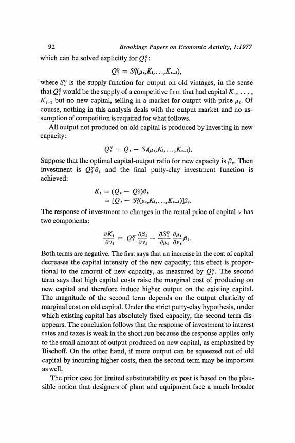
which can be solved explicitly for Q?:

Q? = S?t(pt,Ki, ... jKt_j)j

where S? is the supply function for output on old vintages, in the sense that Q? would be the supply of a competitive firm that had capital K1, .... Kt-l but no new capital, selling in a market for output with price Itt. Of course, nothing in this analysis deals with the output market and no assumption of competition is required for what follows.

All output not produced on old capital is produced by investing in new capacity:

Q7 = Qt -St(AtjKj,...Kt_j).

Suppose that the optimal capital-output ratio for new capacity is pt. Then investment is QNpt and the final putty-clay investment function is achieved:

Kt = (Qt - Q9)O3t = [Qt - St(tK,...Kt_,)]ot.

The response of investment to changes in the rental price of capital v has two components:

-Kt = QN dAt OS_ S 9 t

OVt t Ovt O/.Lt Ovt

Both terms are negative. The first says that an increase in the cost of capital decreases the capital intensity of the new capacity; this effect is proportional to the amount of new capacity, as measured by Qt. The second term says that high capital costs raise the marginal cost of producing on new capital and therefore induce higher output on the existing capital. The magnitude of the second term depends on the output elasticity of marginal cost on old capital. Under the strict putty-clay hypothesis, under which existing capital has absolutely fixed capacity, the second term disappears. The conclusion follows that the response of investment to interest rates and taxes is weak in the short run because the response applies only to the small amount of output produced on new capital, as emphasized by Bischoff. On the other hand, if more output can be squeezed out of old capital by incurring higher costs, then the second term may be important as well.

The prior case for limited substitutability ex post is based on the plausible notion that designers of plant and equipment face a much broader

Robert E. Hall 93

set of alternatives than the users of the capital after the designer has made a specific choice and the equipment is installed. In the extreme, designers decide how many work stations, how many electric motors, and so on, are required to accomplish a certain purpose, and the installed facility cannot operate without the specified labor and electrical input and cannot use extra labor or electricity. The view that most capital has this characteristic underlies the belief that the strict putty-clay hypothesis is a good approximation to reality, though none would argue that it is absolutely precise.

There is an equally strong prior case against the hypothesis. The idea that most of the cooperation between labor and capital takes the form of workers tending machines in a routine way specified by the designer of the machine describes only a small and shrinking sector of a modern economy. In 1973, only 13 percent of the U.S. labor force were classified as operators of machines (other than vehicles). The modern electronic computer is a good example of the case in which few important decisions about the relation between capital and labor are made irrevocably at the time of design. Every user of a computer makes choices constantly about the substitution of the computer's services for human effort. When an investment credit or other influence makes computer services cheaper, computers become cost effective in tasks that had been at the margin. For this substitution, existing computers are just as good as new ones. More generally, the observation that the number of workers tending a machine is largely predetermined by the designer does not establish the putty-clay hypothesis, since the important dimension of substitution may be between the machine and its crew and labor that cooperates without working at a sta- tion on the machine. In the example of the computer, the kind of substitution ex post that refutes the putty-clay hypothesis is not between the computer and its operators, but between the package of the computer and operators, and all of the workers involved in handling data in an enterprise.

Beyond the general objection that the putty-clay hypothesis has an ex- cessively narrow view of the opportunities for substitution ex post, there is one rather specific objection that is fatal to the hypothesis even as an approximation to reality. One of the most important dimensions of factor substitution is variations in the annual hours of operation of capital. The labor required for the marginal hour of operation must usually be paid a weekend or shift differential, so often capital is used for fewer than the 8,760 hours in a year. When capital becomes cheaper, its optimal annual hours of operation drop, and what amounts to substitution of capital for


labor has occurred. In particular, the price elasticity of supply on existing vintages of capital, identified in the earlier theoretical discussion as the crucial aspect of the putty-clay hypothesis from the point of view of investment theory, is potentially high if shift differentials for labor are not too large and if not too high a fraction of the capital stock is at the corner solution of full-time operation.

Robert Lucas has developed a complete analytical treatment of the production possibilities in an economy with variable hours of capital utilization.26 He points out that variations in hours can give a theoretically sound explanation of three puzzling facts about the U.S. economy: (1) the unit elasticity of employment with respect to output in the short run; (2) the cyclical stability of real wages; and (3) the astonishing level of output achieved at the peak of World War II, far above the limit suggested by any simple production function. The theory explains the proportional relation between labor input and real output as reflecting variations in the annual hours of operation of the existing capital stock. The theory does not have a definite prediction about the behavior of the average real wage (averaged across workers paid regular wages for the first shift and a higher wage at other times), but constancy is perfectly compatible with it. Finally, World War II was a period of peak utilization of almost all types of capital. This level of utilization was economically efficient only under the extreme conditions of the war, and would never be reproduced by the private economy in normal periods.

All in all, superficial arguments in favor of the putty-clay hypothesis do not survive careful scrutiny. Higher prices may well bring forth substantial additional output from the existing capital, and this refutes strict putty-clay even as an approximation. The question becomes an empirical one, with no strong prior in favor of putty-clay. So far as I know, the con- nection between the behavior of marginal cost in the short run and the putty-clay hypothesis has not been exploited in empirical work, though it seems a promising approach. The only full-scale empirical investigation of the hypothesis in which it is testable rather than maintained is in Charles Bischoff's work on investment, to which I now turn.

BISCHOFF 'S INVESTMENT EQUATION

In a series of important papers, Charles Bischoff has fitted an investment function in which different distributed lags apply to real output and

26. Robert E. Lucas, Jr., "Capacity, Overtime, and Empirical Production Func- tions," American Economic Review, vol. 60 (May 1970), pp. 23-27.

Robert E. Hall 95

to the service price of capital.27 One of his principal motives was to test the putty-clay hypothesis, which he interpreted as predicting a longer lag between changes in the service price and the response of investment, compared with the lag for changes in output. His results show a strong asymmetry in the two responses and have been widely cited as confirming the putty-clay hypothesis. Representative results from Bischoff's work appear in table 2.28 To interpret his findings calls first for understanding the implications of the use of gross investment as the dependent variable. Sup- pose for simplicity that the capital stock is related by a distributed lag to a variable, Xt, that indexes the demand for capital:

Kt E oiXt_1. i=O

Now gross investment is the sum of net investment Kt - Ktl and de- terioration, 8Kt-l:

It = K - (1 -6)Kt1;

so a function for gross investment is

It = 2 i[Xt - (I -6)Xt-i-1].

The analog of Bischoff's procedure for this simple model would be to fit a distributed lag to the levels of Xt:

It = Xt_i.

The lag parameters ,/3 and ,1 are related by

i'= i- (1 -a)i

However, the level form is more general in one central respect: in the difference form, the function is constrained so that net investment depends only on the first differences and not on the long-run level of demand, while in the level form this basic conclusion of investment theory can be vio-

27. "Hypothesis Testing and the Demand for Capital Goods"; "Effect of Alterna- tive Lag Distributions"; and Charles W. Bischoff, "Business Investment in the 1970s: A Comparison of Models," BPEA, 1:1971, pp. 13-58.

28. I calculated these from the data in the appendix to his paper, "Effect of Alternative Lag Distributions." They do not agree exactly with any of Bischoff's published results, but the difference is unimportant. In the process of this work, I verified Bischoff's claim that his findings are extremely robust with respect to the choice of lag specification. Even specifications that take a very different approach to fitting separate lags for output and the service price of capital showed the same strong asymmetry reported by Bischoff.


Table 2. Bischoff's Investment Function in Level and Difference Form

Equations

2.1 Level forma 11 11

it 'Vtei Qt-i + 7A Vtii Q _i

,B= -0.165 yA = 0.177 (0.026) (0.026)

2 0.9918 standard error = 0.637

2.2 Difference forms 10

it = I Sit V_i Q t-i -(1 -) t_iiQ t-i-l i=o

10

+> 'Yi[Vt-i_1Q t-i-(I - 6) Vt-i2Qt-i-11 i=o

gi = -0.465 EYi = 0.604 (0.140) (0.138)

k2 = 0.9215 standard error 1.972

Lag coefficients

Level form, 2.1 Difference form, 2.2

Service-price Service-price Lag Output effect, effect, Output effect, effect,

(quarters) ,B '+ y ,B' + 1Y-I f3i + yi 13i + Yi-1

0 0.012 -0.002 0.019 -0.010 1 0.008 -0.001 0.009 0.008 2 0.004 0.001 0.003 0.002 3 0.001 0.001 -0.001 0.002 4 -0.001 0.002 -0.003 0.004 5 -0.002 0.002 -0.003 0.004 6 -0.002 0.002 -0.003 0.006 7 -0.002 0.002 -0.001 0.006 8 -0.001 0.003 0.002 0.005 9 -0.001 0.002 0.011 0.004

10 -0.001 0.001 0.002 0.006 11 -0.003 -0.001 -0.016 -0.008 12 0.000 0.000 0.000 -0.022

Sources: The lag coefficients are representative results calculated from data in Charles W. Bischoff, "The Effect of Alternative Lag Distributions," in Gary Fromm, ed., Tax Incentives and Capital Spending (Brookings Institution, 1971), pp. 128-30.

a. It = gross investment; Vt inverse of real service price of capital; Qt = real output; a = quarterly depreciation rate, assumed to be 0.04. Standard errors are in billions of 1958 dollars.

lated. In terms of the lag parameters, 8B of the level form, this restriction is

2 (1- -ig' = Q. This linear restriction on the regression coefficients can be tested with

Robert E. Hall 97

standard techniques. If it is rejected in favor of a positive value of the weighted sum, then net investment depends on the level of the demand for capital even in the long run, and the equation cannot be called an investment function. Again, the obvious interpretation of this finding is that the disturbance in the investment equation is correlated with the right-hand variables.

As the equations in table 2 show, Bischoff actually fits separate distributed lags to composite variables that are the products of his relative price of capital services, Vt, which contains the service price in the de- nominator, and real output, Qt. In this case, in order to qualify as an investment function, both sets of distributed-lag coefficients should satisfy the constraint; in other words, Bischoff's investment equation ought to look like equation 2.2. The results in table 2 show that Bischoff's equation is devastated by the constraint that it be a genuine investment equation. The unexplained residual variance rises by a factor of more than nine, from less than 1 percent to almost 8 percent.29 The problem with Bischoff's equation can be seen in the first two columns at the bottom of table 2, where the separate influence of output and the service price of capital are computed for the unconstrained equation. Most of the positive effect of output is in the contemporaneous quarter or in the immediately preceding quarter. Eventually the influence becomes negative, but the negative coefficients are nowhere near large enough to counteract the strong contemporaneous effect. As Bischoff emphasizes, the pattern of response to the service price of capital is very different: it starts at zero, builds to a peak, and then subsides. But only three of the coefficients are negative; the equation has the erroneous implication that a permanently lower interest rate makes net investment permanently higher. The explanation for this finding is not transparent, but it is plainly incompatible with the most general principle of investment theory.

The third and fourth columns of table 2 show the results of constrain- ing the coefficients to eliminate permanent effects on net investment. The contemporaneous relation between output and investment remains strong, but the negative part of the distribution comes earlier and is stronger. The

29. Now it is clear why Bischoff's equation was so dominant in his comparison with other investment equations ("A Comparison of Models"). The equations based on Jorgenson's work do embody the constraint and so run under an enormous handicap. Most of Bischoff's victory is attributable to this handicap and not to the separate distributed lags he fits.


effect of the service price remains very different; Bischoff's central argument that output and the service price are related to investment in rather different ways is strongly sustained in these results. But there is no reason to believe a priori, and no evidence in these results, that imposing the theoretical constraint somehow completely overcomes the problem of simultaneity. The negative weights at the very end of the distribution for the service-price variable are particularly suspect: theory permits them to be zero but not negative.

Another way to express the unsatisfactory nature of Bischoff's results is to compute the value of the depreciation parameter, 8, for which the equation really is an investment function. This can be done separately for the output effects and the service-price effects. The rate of depreciation that achieves 1(6B + y')(1 - 8) - = 0 for the first column of table 2 is 8.6 percent a quarter, or 30 percent per year, far above any reasonable value. Equipment that depreciates this quickly is often not classified as capital at all, in fact. The corresponding calculation for the service-price effects yields the even more unreasonable value of 59 percent a quarter.

Taken at face value, Bischoff's results are by far the strongest challenge to the principal thesis of this paper. According to a corrected version of his equation, about half of the accelerator response of investment to output is estimated to occur within a year while interest effects take much longer. Those results correspond roughly to row 3 of table 1, and thus imply that expenditure policies can have a substantial effect on GNP. However, this conclusion rests on the proposition that the sum of the accelerator and the marginal propensity to consume is almost exactly one, so that the pure expenditure process is explosive or nearly so. This implication of the corrected putty-clay findings has not been widely appreciated and probably makes them less plausible than they appear to be when the equation is studied in isolation. Unfortunately, it appears that a strong correlation between the disturbance in the investment equation and the level of GNP is biasing the equation toward too sharp an initial response to changes in output. Certainly the overwhelming statistical rejection of the accelerator hypothesis points in this direction. Much more study of the investment equation, with a great deal more attention to the critical issue of simultaneity, will be required to give convincing evidence that the accelerator effect is as strong as it appears to be in regressions that follow Bischoff's approach but are made consistent with investment theory. For now, it appears more reasonable to put the first-year effect at no more than 30

Robert E. Hall 99

percent of the long-run effect, rather than the 50 percent figure implied by equation 2.2. This brings the effect of expenditures on GNP into the range of 0.5 to 0.8, rather than the 1.4 implied by that investment equation.

Summary of Evidence on the Three "Qualifications"

This paper has presented evidence bearing on the validity of the three qualifications of the investment process listed at the outset.

LAGS

The evidence does have something to say about lags in the investment process, and they are an important influence in inhibiting the response of investment that would otherwise make the IS curve very flat. Within the class of investment functions in which the same lag applies to both the accelerator effect and the interest-rate effect, the evidence suggests that somewhere between 10 percent and 30 percent of the long-run response of capital occurs within the first year. Investment is very sluggish compared to the aim of stabilization policy. Still, the results in table 1 suggest that the interest sensitivity of investment over the first year is a major influence in weakening expenditure policy and strengthening monetary policy within that period, even when the investment response is at the low end of the range.

PUTTY-CLAY

Neither the strict putty-clay nor the strict putty-putty hypothesis seems plausible, but research has not uncovered the right compromise between them. To the extent that putty-clay predominates, both expenditure and monetary policies have major effects within the first year, because the accelerator effect acts well before the inhibiting interest-rate effect. Con- sistent regressions that correct Bischoff's approach support this view, but strong evidence of simultaneity undermines the usefulness of those results. The sharp accelerator response of investment in the first year after output changes is an unreasonable feature of the equation quite apart from the more complicated criticism offered earlier in this paper. It is the strong


accelerator, much more than the weak interest response, that makes expenditure policy so powerful with that type of investment equation.

TERM STRUCTURE OF INTEREST RATES

As a matter of theory, what belongs in the service price of capital is a short-run interest rate, though the issue of short against long rates is un- likely to be resolved empirically. But this is hardly the end of the story. A more general question, quite beyond the realm of the investment equation, is the relation between the short-run interest rate appropriate for investment decisions and the market return to short-term financial assets that is appropriate for decisions about holding money.30 The traditional view, adopted in the simple IS-LM model at the beginning of the paper, is that interest-bearing financial assets and real capital are close substitutes, and money is a weak substitute for either. Then markets should equalize the short-run yields of all nonmoney assets, and the common yield is what belongs in the investment equation. If the various kinds of assets, real and financial, are not close substitutes, there is no reason to expect markets to equalize yields. In particular, the yield from a very money-like financial asset, say Treasury bills or commercial paper, is not a good guide to the market's short-run interest rate or net yield from real capital. A better choice might be the expected short-run yield from long-term financial assets. This line of argument does not seem to suggest that the long rate itself belongs in the investment equation, however. Further, it does not have any definite implication with respect to the basic issue of the interest elasticity of investment and the effects of alternative stabilization policies.

Conclusions

Economists do not seem to be ready to make precise statements about the effects of stabilization policies on gross national product. This paper has focused on the role of the investment process in stabilization. The IS-LM model makes it clear how important the negative response of investment to interest rates is in limiting the effect of expenditure policy and providing the principal immediate effect of monetary policy. Empirical evidence on the interest and accelerator responses of investment is weak,

30. I am grateful to Benjamin Friedman for a helpful discussion of this point.

Robert E. Hall 101

however. The calculations at the beginning of the paper do suggest that the conventional estimate for the effect of expenditure increases-about $1.5 billion in GNP in the first year for each $1 billion of expenditure-is probably on the high side. Indeed, perfectly reasonable assumptions give rise to effects only half as large. A hard look at the limited evidence on the IS curve makes exclusive reliance on expenditure policy seem an unwise approach to stabilization.

The same factors that make one policy weak make the other strong. Given the uncertainty about these factors, especially about the slope of the IS curve, it would make sense to adopt balanced combinations of stabilization policies. The negative covariance of the effects of the policies would make the uncertainty about the effect of the total package less than the uncertainty about any individual component. The design of stabilization policies needs to protect against the very real possibility of a flat IS curve.

APPENDIX

Parameters of the IS-LM Model

THIS APPENDIX outlines the derivation of the parameters of the IS-LM model used in the text.

Consumption Function

To get rough estimates of the marginal propensities to consume out of gross national product, I simply ran two regressions of the first difference of real consumption of nondurables and services and the first difference of real expenditures on durables on the first difference of real GNP for the years 1950-76. The resulting coefficients (actually the sum of the current and three lagged quarterly coefficients) were 0.20 for nondurables and services and 0.16 for durables, so 01 is taken as 0.36.

102 Brookings PaDers on Economic Activity, 1:1977

Money-Demand Function

Research on money demand is currently in an unsatisfactory state because of the puzzling behavior of interest rates relative to income and the money supply in 1976 and 1977. Stephen M. Goldfeld's careful investiga- tions of money demand both before and after the puzzle appeared are difficult to embed in a simple LM curve.31 First, Goldfeld finds consistently that the income elasticity of money demand over a one-year period is less than 1/2. The result is a startlingly large shift in the LM curve for each billion dollars of monetary expansion: at least a 2 percent increase in income is necessary to hold interest rates constant in the face of a 1 percent increase in the money supply. Goldfeld's low income elasticity arises from the pronounced downward trend in M, relative to GNP. Since there is no other trend variable in his equation, the coefficient of log GNP is determined largely by the requirement that the rate of growth of real money demand is about half as high as the rate of growth of real GNP. Adding a time trend to his equation increases the estimated income elasticity substantially, to almost 0.8. Second, Goldfeld's most important interest rate is the yield on time deposits at banks, which is not likely to respond very much to monetary or fiscal policy.

In an effort to sort out these two problems in adapting Goldfeld's equation for the present purposes, I fitted the following regression to annual data for M. for 1954 to 1976:

log M/p = 0.56 + 0.78 log Y - 0.014 log r - 0.021t. (0.86) (0.14) (0.13) (0.005)

A2 = 0.94; standard error = 0.013; p = 0.81.

The numbers in parentheses are standard errors. The single interest rate here is the yield on four- to six-month commercial paper. Variants of this equation, including the use of quarterly data, produced similar results. In all cases, the statistical evidence in favor of the trend is unambiguous and the inclusion of the trend dramatically increases the income elasticity. It also reduces the interest elasticity, which in all cases was smaller in magnitude than Goldfeld found.

At probable 1977 levels (GNP of $1,325 billion and money supply

31. "The Demand for Money Revisited," BPEA, 3:1973, pp. 577-638, and "The Case of the Missing Money," BPEA, 3:1976, pp. 683-730.

Robert E. Hall 103

of $230 billion, both in 1972 prices), the income elasticity of 0.78 implies that an increase of $1 billion in GNP will raise money demand by $0.135 billion. This income effect was used in the IS-LM model (, = 0.135). The regression implies that an increase in the interest rate of 100 basis points, from 5 percent to 6 percent per year, will reduce real money demand by $0.59 billion. By contrast, in Goldfeld's basic equation ("Case of the Missing Money," table 1, first line, p. 686), an increase of the same amount in the commercial paper rate alone raises real money demand by $1.84 billion. If both the commercial paper rate and the rate on time deposits increase by 100 basis points, real money demand rises by $6.13 billion, according to Goldfeld. As a compromise I took the interest-rate parameter of the IS-LM model ('2) to be 2.00.

Comments and Discussion

Christopher A. Sims: Hall argues for the view that capital is homogeneous and flexible, for practical purposes, and that therefore price incentives can be effective in stimulating investment even when output is below trend. This is to be contrasted with the perhaps more widely accepted view that at low points of the cycle excess capacity forms a heavy cloud over investors' spirits, preventing price incentives from brightening things much. Hall's view is internally consistent and broadly consistent with the existing statistical evidence, in my view. Where I may differ from Hall is in thinking that the "excess capacity as a heavy cloud" view is equally consistent internally and consistent with the statistical evidence. The truth is, as Hall makes apparent, we don't know much about some of the critical issues related to evaluating the effects of monetary and expenditure policy on investment.

The central question is whether it is reasonable to treat new and old capital as technically interchangeable. There is no solid statistical evidence that the cost of capital strongly affects investment (as opposed to long-run capital stock), in my view. Estimates that claim to have found such an effect fall into two classes: those using models in which output and cost-of-capital effects are tied together a priori, and those in which equity prices are introduced into the formula for the rental price of capital. If capital adjusts very slowly to its equilibrium value, one expects to see investment showing strong positive correlation with stock prices, because both investment and stock prices will reflect expected future yields. Thus a strong negative "effect" on investment of the ratio of dividend yield to equity prices is not strong evidence against a view that investment is price inelastic. But this appears to be the only kind of evidence available in empirical work.

104

Robert E. Hall 105

Hall is right to suggest that identification problems might well completely explain the erratic behavior of cost-of-capital variables in investment-equation regressions, however.

In the absence of conclusive statistical evidence, Hall presents three arguments that vintage effects are negligible. In evaluating these arguments, it is important to have in mind the correct condition that will allow vintage effects to be ignored. Franklin Fisher developed that in a 1965 article in Review of Economic Studies: at any one time capital of all vintages must have the same gross margin. This condition is a little weaker than Hall's condition that their marginal products differ only by an ex- ponential depreciation factor. One can easily imagine examples in which the Hall condition is violated-for instance, in any situation in which investors expect that capital currently being purchased will all be replaced at roughly the same time. Hall's first argument for negligible vintage effects, that it is "hard to think of realistic conditions" under which Fisher's conditions are violated, is therefore unconvincing.

The Fisher capital-aggregation condition is exactly what Hall needs for his argument early in the paper that short rates are all that matter in the investment function. Later in the paper, Hall argues that it is the price elasticity of output on old equipment that determines the degree to which investment responds to changes in the price of capital. While it is true that the price elasticity of output could be high on old equipment even though Fisher's aggregation condition is not close to being true, Hall's argument is incomplete. The response of investment to capital cost depends on the response of price to capital cost (Hall's dju/dv) as well as on the response of output on old equipment to price. If average variable cost on old equipment cannot be radically reduced by reducing output on the old equipment, one gets the commonsense result that changes in the short interest rate that are not expected to persist have little effect on investment, even if output on old equipment is price elastic. Hall's second argument, that vintage effects are negligible because the price elasticity of output on old equipment is high, therefore founders on his having failed to consider vintage effects on d,u/dv.

Hall claims that the positively sloped IS curve that emerges from his version of Bischoff's equation is a priori implausible. Perhaps because of a deficiency in my stock of a priori knowledge, I find this third argument unconvincing as well.

Now for some other issues. On the short versus the long rate: If capital


is in infinitely elastic supply and investment is reversible, it is hardly surprising that a short rate is what matters for such a liquid asset. If putty-clay effects are important, the whole term structure is relevant. Even without putty-clay effects, if capital is in inelastic supply, the expected rate of change of the price of capital goods enters the service cost. The expected rate of change is not derivable from the history of capital- goods prices in general, and in fact, under some assumptions, may be embodied in the gap between the long and the short rate.

Expectational lags are not so easily handled as Hall suggests. First, if the autoregressive structure of "desired capital" is not second-order Pascal as in Hall's example, it could easily happen that expectational lags lengthen rather than shorten the estimated lag distribution relative to the physical- lag distribution. More important, expectational lags for either the cost of capital or output will in general involve both variables. Thus relative sizes of sums of coefficients in distributed lags bear no necessary relation to the policy-relevant price and output elasticities.

Measurement error, on which Hall relies to cast doubt on the small coefficients in the "q theory" regressions, does not in fact create a bias of determinate sign here. It seems quite likely that fluctuations in the stock market's evaluation of intangible capital are positively correlated with fluctuations in the stock market's evaluation of tangible capital. Thus measurement-error bias from this source might actually tend to inflate rather than reduce the estimated coefficient on q.

Hall is right to suggest that simultaneity problems are probably critical to what comes out of "'investment" or "saving" function regressions. Hall's idea for testing for simultaneity is not a good one, however. The idea that long-run effects of output on net investment must be zero is plausible in a model with static technology. But the underlying reason is that in such a model stationary fluctuation in output cannot plausibly lead to unbounded variation in capital-output ratios. It is also implausible, however, that with static utility functions and stationary fluctuations in income, desired wealth-income ratios wander unboundedly. There is no carefully worked out theory of saving that implies a relation of the level of saving to the level of output in the long run. Thus there is no good argument that simultaneous-equations bias will bias sums of coefficients on output in net- investment equations away from one.

So where does the levels relation come from? In part, from statistical artifact. Plausible assumptions suggest that the negative part of the lag

Robert E. Hall 107

distribution on output should be long and flat. It is easy to show that such long, flat, low tails are difficult to estimate, and that there is likely to be a strong temptation to truncate the lag distribution before the long thin tail and end up with only the short, fat, positive part. Also, in reality, non- stationary movement in technology may occur. And finally, Hall claims to adapt his test for a stable capital-output ratio to a gross-investment equation under general putty-clay assumptions; but in a general putty- clay model there is no exogenous, fixed rate of depreciation. Since Hall's adapted test rests on use of a fixed depreciation rate, its interpretation is at best debatable.

Franco Modigliani: By way of introduction, I should explain that, as MIT colleagues, Robert Hall and I agreed to avoid praising each other, and instead to take our gloves off.

When I tried to formulate my comment on this paper, I recalled the famous fable by Edmund Phelps in his classic paper on the golden rule, and I shall use a similar tale. I imagine that the prince of the realm de- cides one night that he wants somebody to show that fiscal policy is powerless and monetary policy very powerful. He asks his adviser, "Who is the most brilliant young economist in the realm to carry out this task?"

The designated man then is asked to do that. He does it with great relish, and finds that it is just his cup of tea. For several months he works as hard as he can, making the case-without violating conspicuously the rules of the game. The outcome of that effort is now before us.

It is full of interesting and challenging ideas, even though it is some- times irritating, and even though it takes several days to read it because the reader has to be careful about what might be slipped by him. But for all its brilliance, I doubt that it will persuade many that the first year's effects of fiscal and monetary policy are, respectively, as puny and as gigantic as they are reported to be in table 1!

But let us follow our hero on the path that leads to table 1. Of course, the brilliant young man knows that, to make monetary policy powerful and fiscal policy powerless, it takes a very steep LM curve and a very flat IS curve. He further knows that three factors stand in the way of a flat IS curve. One is adjustment lags; the second is the putty-clay technology; and the third is the fact that money affects short-term interest rates promptly and directly, while investment depends on long-term interest rates.

Brookinps Paners on Economic Activity. 1:1977

I need not say much about the first issue, the lags, because even our brilliant economist, after all, cannot budge the finding of substantial lags, whether these be due to putty-clay or other reasons.

A major novelty in Hall's attack is his criticism of the traditional view that investment depends on the long-term interest rate. He argues, instead, that the only rate that matters is the short-term interest rate.

One may well accept the proposition that short-term interest rates may matter for investment. Stephen Marglin once argued, quite rightly, that a single investment project must meet two tests. One is the long-run test: it must be profitable at the current long rate. If it meets that test, the next question is, "Could it be profitably postponed?" That answer depends, essentially, on the relation between the current short and long rates. If the project meets the first test, but the short rate is too high, it may be worth- while to postpone, because the project will not pay for itself in the near future.

If, on the other hand, the short rate is below the long rate, then the second test is immaterial because any project that meets the long-rate test will also beat the short rate. It is only when the short rate is above the long rate that the double test applies. In early work on the MPS model, we looked for evidence that short rates mattered when they were above long rates. We did not get any significant results, but in principle that is a valid point.

But how can one claim that only the short rate matters? One possible way is to imagine that capital is just putty: the firm has a certain quantity of it, but it can dispose of as much as it wants in the next period. Clearly, if the firm can resell the putty in the next period at a known price, it need only be concerned with the interest cost for the current period-that is, the short rate. But our economist makes a far more general claim. He con- tends that with putty-putty technology it is immaterial whether or not the capital goods can be readily resold. Actually, this claim can be shown to be valid only in one special case-namely, on the assumption that the quantity of "putty" capital that the firm is considering holding today on the basis of the short rate is less than (or at least not more than) the quantity it would want to have tomorrow, after allowing for the depreciation between today and tomorrow. Under these circumstances, the firm makes a decision now that has no bearing on what it will have tomorrow, because tomorrow it can add whatever is needed. In that event, our economist is

Robert E. Hall 109

absolutely right: only the short-term rate will matter. In principle, the one-day rate is all that is needed to decide on the amount of capital to hold each day.

The mere fact that the putty-putty model can lead to this absurd consequence is a good reason why it makes no sense. As soon as putty-clay characteristics are recognized, the whole argument disappears, and investors have to worry about the whole future path of interest rates. In particular, especially when one recognizes limited ex post substitution, it will normally be the case that for long-lived investments what matters is the long-run interest rate-except when the short rate is so much above the long rate that it may be a sufficient barrier to investment. One wonders whether Hall is really serious when he states that it is "clear that the service price of capital depends on the short-run interest rate."

Since the argument about the short rate rests to a large extent on putty-putty, our author has to destroy the competing putty-clay hypothesis. That attack takes many forms in the paper. First he sets forth a number of arguments, old and new, as to why there may be significant ex post substitution between labor and capital. As far as I can see, the most relevant one is that even though the ratio of plant to labor may be fixed per unit of time, the substitution can occur by way of varying the number of hours per year that a plant is combined with labor; thus a higher rental rate for capital might well, in principle, lead to introducing an extra shift. But, even granting the validity of this argument in principle, I would expect the elasticity of substitution through this mechanism to be quite small because of extreme discontinuities. To be sure, in the short run one can change utilization through overtime and some extra shifts; but in the long run, one must basically operate with one shift or two (or three), but cannot respond to a 10 percent rise in the rental rate by adding a small fraction of a shift. On the whole, I see Hall's arguments as merely providing one more illustration of the proposition that nothing in economics is ever completely black or white. If asked: "Is there never any ex post substitution between capital and labor?" I would have answered: "Never? Well, hardly ever!" After Hall's paper, my answer remains pretty much the same.

But the main attack on putty-clay takes the form of a severe critique of the major empirical work in this area, which is that of Bischoff. As a preliminary to that attack, our author argues that, when investment is


expressed as a function of a distributed lag on income, estimates of the parameters of the function may be biased. We all know that, when there is simultaneity, this problem does exist to some degree.

With this background, Hall goes into a rather technical and lengthy discussion of results of a Bischoff-type equation fitted by him using actual investment, ignoring several other existing putty-clay equations based on new orders and hence less subject to simultaneity bias (for example, that of Ando, Modigliani, Rasche, and Turnovsky in International Economic Review, in June 1974). He argues that his Bischoff-type equation implies either an unrealistically high rate of depreciation or else that net investment depends on the level and not merely on the rate of change of (desired) output. From this he concludes that the equation must be subject to bias so severe as to make it of little relevance, except possibly for further study.

My interpretation of his results is rather different: the coefficients of his equation imply merely that the accelerator effect-the cumulated response of net investment to a step change in output-is somewhat on the low side compared with the long-run response of gross investment to a constant level of output, which represents, of course, replacement investment. This conclusion turns out to hold also for the equations of Ando and his associates, mentioned above, though in lesser degree. As noted by Hall, the two responses can be reconciled by assuming a sufficiently high rate of depreciation. But even for Ando and his colleagues, the required rate is above 7 percent per quarter, which is not very realistic. One must agree, therefore, that the estimated coefficients are likely to be somewhat biased. However, Hall concludes, without apparent justification, that the bias consists in an overestimate of the (long-run) response to the level of output. My own calculations, on the other hand, suggest that this long-run response is broadly consistent with a reasonable depreciation rate and the average capital-output ratio; the bias is, instead, in the estimated accelerator response which is somewhat low. There is no reason to believe that this bias is particularly related to simultaneity-especially when the dependent variable is new orders. A more likely major explanation is at- tenuation due to errors of measurement, including misspecifications of some of the independent variables. This is but a small blemish for a rather complex, highly nonlinear, equation that otherwise makes a lot of sense, especially when even Hall's results provide strong confirmation that the pattern of response to output and to the interest rate are quite different, which is the differential implication of the putty-clay model.

Robert E. Hall 111

It is, therefore, good that in table 1 Hall has provided estimates of the differential policy implications of putty-clay as well as putty-putty, though in my view the relevance of this table is most doubtful. In the first place, Hall's estimates of the putty-clay response are rather arbitrary. The estimates of Ando and his associates suggest a slower accelerator response in the first year, especially after allowing for the lag of deliveries behind orders. Hall's assumption of one-eighth response to interest rates is nowhere explained, but seems high. Under putty-clay, the response is related basically to the depreciation rate, and for total investment that rate is likely to be rather less than one-tenth. But the main factor that puts the results of table 1 beyond the pale, in my view, is the combination of the following assumptions, which are questionable individually but plainly incredible taken together. The first is the crucial assumption-designed to insure a very steep LM curve and defended most unconvincingly in an appendix-that the demand for money is extremely interest inelastic, and hence short-term interest rates are extremely volatile; a 1 percent change in the money supply is assumed to reduce the short-term rate by roughly 25 percent, while a 1 percent rise in real income increases it by over 15 percent! These estimates are many times larger than those implied by Goldfeld's money-demand equations or, even more by the MPS's. All of the extreme results of table 1, especially with respect to changes in M1, become readily understandable when one recognizes that this first assumption is combined with two more: (1) that investment decisions respond exclusively to that volatile short-term rate-specifically the rate on four- to six-month commercial paper; and (2) that through putty-putty, a change of 100 basis points in that rate will produce promptly investment of $84 billion (in 1972 prices)!

No wonder that, for most of the cases considered, a change in M1 produces an ultra-monetarist first-year effect close to, or even larger than, the current velocity of circulation, whereas fiscal policy can hardly get off the ground.

Finally, let me mention one general complaint about the relevance of the comparisons between fiscal and monetary policy presented in table 1, even if I thought the entries in the table had any empirical relevance. I submit that whenever we look at the effects of stimulative changes in taxes and government expenditures, what must be kept constant is the interest rate, not the money supply. Why would anyone want to keep the money supply constant if the objective is to stimulate the economy? And


this should hold with special force for those who believe in the potency of money. Only if the government is trying to increase its expenditure at the expense of investment should it keep the money supply constant. But if it is trying to increase income-and not to reduce investment or to increase interest rates (for balance-of-payment reasons, say) -then it would just waste part of its effort by keeping the money supply constant.

In the present state of the economy, for instance, we ought to have expansionary monetary policy and expansionary fiscal policy, and stop the nonsense about the fear of inflation being linked to monetary growth. If inflation is the main worry, we should not want any stimulation. If we want stimulation, we should use monetary policy to reinforce and not to offset fiscal policy.

By the time I was through with the paper, I actually felt relieved. I had been exposed to the most serious and brilliant attack I could imagine on several issues on which I have strong convictions, like the importance of the long rate, putty-clay, a first-year fiscal multiplier in excess of one. I was glad to see that my views came out basically unscathed by this paper.

William Brainard: I want to comment on James Tobin's theory of investment which Hall describes as a major competitor to Jorgenson's theoretical framework, and to offer some observations about the Jorgenson- Hall theory. One major feature of Tobin's approach is its stress on the difference between the required return to capital and the return on financial assets. The reasons include differences in maturity, but perhaps more important, encompass differences in various types of risk-of inflation, of default, of changing demand and technology.

In order to understand the mechanism by which monetary policy or other financial events affect investment it would be desirable to have a direct measure of the required rate on capital. Such measures are difficult to come by precisely because the distinctive uncertainties on capital mentioned above make it hard to identify its expected profitability. Empirical work by Tobin and myself and by Modigliani, as well as evidence on the historical return to investment, suggests that the required rate on capital is not only substantially higher than the required rates on bills or bonds, but is far from perfectly correlated with them.

Tobin's q model of investment, empirically implemented by John Cic- colo of Boston College, shortcuts the need for a separate calculation of expected profitability and the required rate. Although variations in q re-

Robert E. Hall 113

flect changes both in the required rate of return and in the market's calculation of marginal profitability, their separate identification isn't needed if firms are behaving in accordance with the q model. Firms will invest when the securities market places a high value on investment relative to its cost. The financial markets do the job of calculating for them.

Why don't firms adjust their capital stock instantaneously to maintain the equilibrium value of q? This is analogous to the classic question of why investment demand should remain finite with changes in the interest rate. Tobin's view, in common with that of many other writers, is that costs of adjustment of the capital stock, both to the firm and to the economy, are important elements in the explanation. Hall is right, however, in suggest- ing that adjustment costs are not a necessary feature of the q model. One could accept that model without believing that the adjustment costs are important, or believe the costs are important without accepting a formulation that works through the financial market's valuation of capital goods. In principle, in a competitive world, increasing costs and capacity limitations in the construction and capital-goods industries show up as a rising supply price of capital goods, and do not enter the investment- demand equation. To make sense of many macro models one has to assume that such supply considerations are unimportant, or that they are implicitly incorporated in the investment "demand" equation or schedule. Hall objects to inclusion of supply considerations in the aggregate-demand equation, but does not claim that they are unimportant to understanding the level of investment. He owes us either an explicit justification for ex- cluding flow considerations from the supply side, or a capital-goods supply equation in his model. Indeed, if because of costs of adjustment internal to the firm or some other reason firms need to predict the price of capital goods, the supply side is relevant to investment demand. For example, if firms are aware that the supply price is a function of operating rates in the capital-goods industry, then they are likely to view the existing relative prices of capital goods as unusually high (low) when operating rates of that industry are extremely high (low).

Hall follows Jorgenson in building the theory of investment around the concept of the service price of capital. According to Hall, it is quite unambiguous that the service price should be based on the short-term rate of interest. In the absence of markets for used capital goods a crucial element in the argument is that firms never have to worry about getting stuck with excess capital; they are assumed always to want more capital


tomorrow anyway. At the aggregate level that has been true since the Great Depression, but aggregation conceals the variation of experience among firms. It seems fair to say that any firm that goes bankrupt, or finds itself boarding up windows, should have been worrying about that possibility when it undertook investment. The problem for the firm is exacerbated by the heterogeneity of capital goods. A firm that is buying new trucks may have too many machine tools. If I ever find a corporation that be- haves in the Jorgenson-Hall fashion, looking only one year ahead in making twenty-year investments and responding only to the current bill rate, I'll sell short. Aggregation, of course, can conceal-even mitigate-a multitude of sins, but I see no reason to believe that the profit-maximizing behavior of a firm assumed to have the characteristics of the aggregate should be a good approximation of the aggregate behavior of individual firms which face imperfect capital-goods markets and invest in specific types of capital. - Hall and Jorgenson give the impression that it is straightforward to

construct a theory of investment around the concept of a service price of capital which also includes a distributed lag of investment in response to its determinants. In fact, it is quite a trick. It is difficult if not impossible to find conditions that justify the use of the service price of capital based on the short rate and yet allow for the many circumstances that prevent the firm from continuously equating the actual to the desired stock of capital. Hall follows Jorgenson in assuming that the process of designing, ordering, and installing capital follows a fixed time schedule. In my view, adjustment costs are the explanation of the implied lags, rather than an alternative explanation, as Hall states. In a theoretical investigation I am reluctant to treat the lags as entirely mechanical rather than the consequence of an economic calculation. Assuming they are mechanical, however, why doesn't the Jorgenson-Hall firm manipulate orders to keep capital precisely on target (assuming that some capital is delivered in the period orders are placed) or on the expected target only the minimum lag away? Hall gets out of that bind by assuming that capital with short delivery lags cannot substitute for capital with longer delivery lags. Types of capital are now defined by their delivery lag! How is it that capital goods that cannot substitute for each other during the investment process end up as homogeneous capital in a Cobb-Douglas production function? If each lag does refer to a distinct type of capital and production process, why is capital of different types purchased in fixed proportions? Why isn't

Robert E. Hall 115

the firm able to place separate orders for each type? Why, therefore, doesn't the "lag distribution" reflect the time pattern of expected needs for capital of various types rather than the mechanical delivery schedule? If capital goods are complements, how can the delivery of capital with the shortest lag affect output and "its" quasi-rent prior to the delivery of com- plementary capital with longer lags?

Hall asserts that his most sluggish investment response in table 1, which assumes one-eighth of the long-run response in the first year, is consistent with Ciccolo's empirical estimates of the q model. Hall's derivation of the relationship between I and q involves a number of assumptions and approximations that prevent one from having much confidence in the asser- tion. Hall ignores the lag of approximately three quarters in Ciccolo's investment equation. In calculating q he does not discount excess quasi- rents, even though some of them are far in the future. This tends to minimize the apparent discrepancy between the desired and actual capital associated with a given q. He calculates quasi-rents separately on capital of "different lags," even though he uses the characteristics of the aggregate production function to estimate the quasi-rents of each type, and then simply adds them up.

It seems difficult to reconcile the observed deviations of q from its equilibrium value with the view that these deviations simply reflect the excess quasi-rents that accrue while delivery takes place. Since 1960, q has ranged from 0.75 to 1.36 according to the Council of Economic Advisers (up to 1.67 according to Ciccolo). The inconsistency of fluctuations of this magnitude and Hall's view can be seen by taking a set of extreme assumptions, all tending to minimize the amount of investment required to restore equilibrium.

Suppose quasi-rents are not discounted, and that the market assumes that current quasi-rents go on forever. Then a change in required rate that increases q from 1 to 1.3 implies (for the Cobb-Douglas) that desired capital is 30 percent greater than actual. If complete adjustment took place in ten years, and the investment was spread out evenly rather than bunched at the beginning, as assumed by Hall, this would imply increasing investment by about 4.2 percent of GNP for each of the ten years (assuming Hall's barely credible capital-output ratio of 1.4)!

In fact, of course, Ciccolo's investment equation implies substantially less investment in the first year than is given by this calculation; and the increase in desired capital implied by an increase in q of 30 percent, tak-


ing account of discounting and the elimination of excess quasi-rents as investment takes place, is much greater than 30 percent--probably something on the order of 60 to 90 percent. The fraction of the long-run response in the first year implied by Ciccolo's equation is more like one- thirty-second than the one-eighth used in Hall's table 1, even ignoring the lags in Ciccolo's equation.

Hall stresses the fact that in his model, no matter how much he waters down his beliefs about the response of investment to interest rates, he gets a small expenditure multiplier and a large money multiplier. This is hardly surprising given the assumed inelasticity of the demand for money and the use of the bill rate in both the demand-for-money and investment equations. Hall's interest elasticity of the demand for money is essentially an average of zero and Goldfeld's estimate, and I assume others will take him to task for the cavalier estimation of this crucial parameter. Of equal importance is his reliance on a single short rate to equilibrate the model. As my comments above indicate, I do not believe there are strong theoretical or empirical reasons for using the short rate in the investment equation. Hall concedes the importance of lags in the delivery of capital goods, and that by itself is enough to rule out a very short rate. On Hall's assumption that the mean delivery lag is about two years, the current three-month bill rate is surely a poor approximation of what he should be interested in, even in terms of his own model. The expected short rate implicit in borrowing long now, and lending long a year from now, is far from perfectly correlated with the bill rate, and even advocates of the expectations theory allow for a risk premium that makes long rates higher than short rates. That concession alone changes the relevant elasticity calculation. If a short rate were to be used, I would not want to use the bill rate or the short rate implicit in the return on other financial assets, but the short-term required rate on capital, which is not likely to be highly correlated with them.

If for either risk or maturity reasons, capital is not a perfect substitute for bills, there will be slippage between the federal funds or bill rates, which are directly affected by monetary policy, and the required rate relevant to the IS curve. The greater this slippage, the less direct and potent is the influence of the Federal Reserve on investment, and the less government expenditures will crowd out private investment. I hasten to add that using the required rate on capital, or some other stock-market vari-

Robert E. Hall 117

able, in the demand-for-money equation would not be the solution. The error is in believing that the rates relevant to these two markets are tied tightly and mechanically together in either the short or the long run.

Robert E. Hall: After a very determined effort to explain why my IS curve is so flat, I learn that what is really the matter-in the view of my critics- is that my LM curve is too steep! Much of the criticism of the paper relates not so much to its conclusions about the investment equation but to the way that equation is embedded in a model of the rest of the economy.

Within the realm of the investment equation itself, some of my discus- sants are worried that the entire theoretical apparatus requires the belief that investment undertaken today will not be so large as to push expected investment next year to zero. None of the marginal conditions that are crucial in my restatement of investment theory are relevant if planned future investment is zero. This is the sense in which the nonnegativity of gross investment is a qualification of the theory. Though I defend the use of a theory that ignores the constraint only as an approximation, I think it is a pretty good approximation. The key issue is not whether investors find themselves regretting past investment, but whether they ever find their planning process constrained by the belief that they will need more capital this year than next year. Reductions in demand are almost always unpleasant surprises.

Christopher Sims raised the point that the use of a service price of capital requires that stringent capital-aggregation conditions hold. Again, I defend the use of a service price as a good approximation to a world in which the conditions do not actually hold. Sims' criticism would be much more convincing if he could give a practical example of a case in which the formula seriously misled an investor.

William Brainard pointed out that investors presumably discount the future excess rents in forming their values of q, and that this would lengthen the implied distribution of delivery lags. He is right, but the magnitude of the bias is small, and I would guess that it is dominated by the bias in the opposite direction caused by measurement errors.

Franco Modigliani and I have discussed the evidence on Bischoff's putty-clay investment function to the point of complete agreement on the facts, particularly that there is an important discrepancy between the short-run and long-run responses of investment to changes in output.


Modigliani defends Bischoff's equation as a workable approximation, while I am concerned about its value as a measure of the importance of the putty-clay phenomenon.

Every reader of the paper seems to have a different reason for thinking that the long-term interest rate belongs in the investment equation in place of or alongside the short rate. William Brainard pointed out that the logic of my model requires that the term of the relevant interest rate be about as long as the delivery lag, not necessarily the same term as is generally used in money-demand functions. He also criticizes the expectations theory of the term structure on which my derivation rests. I would reiter- ate that that theory, in turn, rests on the explicit hypothesis that short and long assets are perfect substitutes. This is good theory, even if the hypothesis is wrong. Franco Modigliani argued that the putty-clay hypothesis completely invalidates my demonstration that only the short rate should matter. The paper concedes this as a matter of exact theory, but claims that the formula based on the short rate is a workable approximation. His statement that putty-clay makes the long rate alone the relevant interest rate for investment is unconvincing to me. Investors face the same issue of optimal scheduling of investment under putty-clay as under putty- putty. Working through the scheduling problem will give the same conditions as appear in my derivation. Then it is just a question of developing a useful approximation.

Modigliani and Stephen Goldfeld (in his remarks recorded below) raise questions about the money-demand function that I use to close the model in order to work out the implications of alternative investment functions. Most of the disagreement relates to my inclusion of a time trend in the money-demand equation, which Goldfeld attacks as unwarranted by theory. I don't know why theory rules out an upward trend in the productivity of the use of money; it seems to me that technical change is just as important here as anywhere. In any case, arguing that the coefficient on the time trend should be zero puts the econometrician in a bind when it turns out to be significantly different from zero. The rest of the disagreement comes from the fairly long distributed lag on income that Goldfeld finds. Why do people take so long to adjust? We disagree least about the magnitude of the interest-rate coefficient in the money-demand function itself. Obviously, my own work in this area is very casual. One of the major lessons I have learned from the discussion is the need for a thor-

Robert E. Hall 119

ough empirical investigation of aggregate asset supplies and demands, including money.

General Discussion

Stephen Goldfeld expressed his dissatisfaction with the LM curve developed in the appendix, which is a critical ingredient in Hall's calculations. He argued that the inclusion of a time trend in the money-demand function was not consistent with theory, according to which the trend in income and in interest rates should explain the trend in velocity. Gold- feld stressed that, despite Hall's "markup" of the interest elasticity in the regression equation, Hall's LM curve was dramatically steeper than the one implied by Goldfeld's results. In particular, Hall's estimates imply that a 1 percent increase in GNP, given M1, raises interest rates by about 17 percent, or about 85 basis points at his illustrative 5 percent interest rate. In contrast, Goldfeld's equations imply a rise of only 15 basis points if both interest rates are allowed to adjust, or 50 basis points if the time deposit rate is held constant. To Goldfeld, the estimates of 15 to 50 basis points provided a plausible bound for the steepness of the LM curve, and Hall's curve clearly lies outside this range.

A number of participants stressed both the importance and the im- plausibility of the assumption in the Jorgenson-Hall model that no investor is ever stuck with excessive stocks of any capital good. In their view, the focus on short-term interest rates and near-term profitability in Hall's paper rested on that assumption. John Shoven pointed out that the overall investment function is an aggregation of micro demands for capital goods; the aggregation makes clear the importance of the composition of aggregate demand, the composition of the existing capital stock, and the variation in rates of depreciation across sectors of the economy. When these various microeconomic factors are recognized, the probability seems overwhelming that at least some firms will be constrained by the zero floor on gross investment. Benjamin Friedman argued that the mere concern by investors that they might be stuck with excessive amounts of capital goods is enough to invalidate the Hall view. He stressed the transactions costs involved in acquiring and financing capital goods, as well as the heterogeneity of capital goods that Brainard had noted. These elements make


liquidity important to a firm and give it cause for concern about the composition of its assets and liabilities. Firms have choices in financing investment among long debt, short debt, and equities, and a further choice on the timing of funding out fixed-investment projects. Friedman agreed with Hall that any theory of investment demand has to simplify these complex decisions. But he disagreed with Hall's strategy of simplification by focusing on the short-term interest rate; in his view, the bond and equity yield would be the preferred place to start. All of this, Friedman con- tended, bore on what he considered to be a key question neglected in Hall's analysis: What is the proper discount rate to apply to expected future returns from the acquisition of a capital good, given that ownership of the capital asset has implications for the structure of the firm's liabilities?

Martin Feldstein reminded the group that the Hall-Jorgenson concept of the rental price or cost of capital is an amalgam, reflecting the interest rate on debts, the dividend-price ratio on equities, and a variety of tax variables as well. Indeed, Feldstein recalled, in some of their initial work the interest rate was assumed constant, and yet the cost of capital varied a good deal because of changes in the tax laws. Feldstein saw no theoretical presumption that investment would respond with equal speed or magnitude to changes in all components of the cost of capital. For example, a change in interest rates and a change in tax depreciation rules might have the same impact on the cost of capital, and yet have different impacts on the optimal replacement decision and hence on scrapping capital goods. Feldstein suspected that, even in a putty-clay world, changes in the cost of capital that affect optimal replacement may lead to especially rapid responses of gross investment. Feldstein also commented that, even if one granted that desired gross investment is always positive, the exclusive focus on short-run calculations would not be justified in a putty-clay technology. If an investing firm locks itself into a particular capital-labor ratio, it must worry about the cost of capital in the future; for one thing, its competitors will be making investments in the future based on capital costs that prevail at the time.

Pentti Kouri contrasted the standard Keynesian theory of investment that he accepted with Hall's formulation. In the standard theory, the capital stock is fixed in the short run, while the valuation of capital is variable; the latter is determined by capitalizing expected returns on investment goods at prevailing interest rates. The values attached to capital assets, in turn, determine the output of new investment goods, given the

Robert E. Hall 121

production costs or supply price of capital goods. In the long run, however, the price of capital becomes essentially constant, matching long-run production costs; meanwhile, the stock of capital becomes a variable and is determined by the demand for capital services. As Kouri interpreted them, Jorgenson and Hall really offer a theory of the demand for capital services, which is thus a theory of long-run capital stock, but not a theory of investment. Tobin, on the other hand, offers a short-run theory of how capital assets are evaluated and thus of how investment is motivated.

In this framework, Kouri saw the short-term interest rate as the key to investment decisions only in the unrealistic case in which the capital stock is completely adjustable-essentially, a liquid asset. In that world, demand and supply for capital services are always in balance and there is no problem in determining investment.

Martin Neil Baily approved of Hall's methodology of focusing on basic issues rather than attempting to distill point estimates from time-series regressions. But Baily shared Kouri's concern about the distinction between capital stock and capital services. In particular, he felt that hours of capital services rather than capital stock should enter into the production function. The decision to use capital for more hours was different from a substitution in technique that altered capital-labor proportions per hour of work.

Edward Gramlich and Lawrence Klein argued that Hall's fiscal multi- pliers were biased downward. Gramlich suggested, first, that the marginal propensity to consume over a full year may be significantly larger than the 0.36 figure used by Hall. Second, he felt that a macro model should allow for an inventory accelerator that is distinct from and more rapid than a general investment accelerator. Klein underlined the critical role of strong inventory responses in American business cycles. He regarded a figure of roughly 1?/2 for the expenditure multiplier over a one-year period as a well-established econometric finding. Replying to Gramlich's first point, Hall found it hard to see how the MPC out of GNP could much exceed 0.36. Even if the short-run MPC out of disposable income were close to one, which few economists believe, the response of disposable income to changes in GNP is sharply limited by taxes and other influences to a value of around one-half. His parameter is the product of these two.

Investment, Interest Rates, and the Effects of ... · The more sensitive the ... the alternative...

Documents

Transcript of Investment, Interest Rates, and the Effects of ... · The more sensitive the ... the alternative...