Hindawi Publishing CorporationJournal of Applied Mathematics and Decision SciencesVolume 2008, Article ID 795869, 13 pagesdoi:10.1155/2008/795869

Research ArticleInvesting in Lead-Time VariabilityReduction in a Quality-Adjusted Inventory Modelwith Finite-Range Stochastic Lead-Time

Farrokh Nasri, Javad Paknejad, and John Affisco

Department of IT/QM, Frank G. Zarb School of Business, Hofstra University, Hempstead,NY 11549-1340, USA

Correspondence should be addressed to Farrokh Nasri, acsfzn@hofstra.edu

Received 22 May 2007; Accepted 11 November 2007

Recommended by Omer S. Benli

We study the impact of the efforts aimed at reducing the lead-time variability in a quality-adjustedstochastic inventory model. We assume that each lot contains a random number of defective units.More specifically, a logarithmic investment function is used that allows investment to be made toreduce lead-time variability. Explicit results for the optimal values of decision variables as well asoptimal value of the variance of lead-time are obtained. A series of numerical exercises is presentedto demonstrate the use of the models developed in this paper. Initially the lead-time variance reduc-tion model (LTVR) is compared to the quality-adjusted model (QA) for different values of initiallead-time over uniformly distributed lead-time intervals from one to sevenweeks. In all cases whereinvestment is warranted, investment in lead-time reduction results in reduced lot sizes, variances,and total inventory costs. Further, both the reduction in lot-size and lead-time variance increase asthe lead-time interval increases. Similar results are obtained when lead-time follows a truncatednormal distribution. The impact of proportion of defective items was also examined for the uniformcase resulting in the finding that the total inventory related costs of investing in lead-time variancereduction decrease significantly as the proportion defective decreases. Finally, the results of sen-sitivity analysis relating to proportion defective, interest rate, and setup cost show the lead-timevariance reduction model to be quite robust and representative of practice.

Copyright q 2008 Farrokh Nasri et al. This is an open access article distributed under the CreativeCommons Attribution License, which permits unrestricted use, distribution, and reproduction inany medium, provided the original work is properly cited.

1. Introduction

The origin of lot-size research can be traced to the development of the square root EOQ formulain the early 20th century. This relationship is the result of classical optimization of inventory-related costs under a series of highly restrictive assumptions. Among these assumptions areinstantaneous replenishment, constant deterministic demand and lead-time, and perfect qual-ity of inventory items. More realistic cases ensue when these assumptions are relaxed. Some of

2 Journal of Applied Mathematics and Decision Sciences

these cases that have appeared in the literature allow for imperfect quality and variability ineither demand or lead-time, or both.

Gross and Soriano [1] and Vinson [2], among others, demonstrate that lead-time vari-ation has a major impact on lot size and inventory costs. Furthermore, they indicate that aninventory system is more sensitive to lead-time variation than to demand variation. The prob-lem of the EOQ model with stochastic lead time has been considered by several additionalauthors including Liberatore [3], Sphicas [4], and Sphicas and Nasri [5]. In this last work, theauthors derive a closed form expression for EOQ with backorders when the range of the lead-time distribution is finite. In this formulation, all units are assumed to be of perfect quality.

Concurrently work has appeared in the literature that relaxes the perfect quality assump-tion. Rosenblatt and Lee [6] have investigated the effect of process quality on lot size in theclassical economic manufacturing quantity model (EMQ). Porteus [7] introduced a modifiedEMQmodel that indicates a significant relationship between quality and lot size. In both [6, 7],the optimal lot size is shown to be smaller than that of the EMQ model. In these works, thedeterioration of the production system is assumed to follow a random process.

Cheng [8] develops a model that integrates quality considerations with EPQ. (Economicmanufacturing quantity.) The author assumes that the unit production cost increases with in-creases in process capability and quality assurance expenses. Classical optimization results inclosed forms for the optimal lot size and acceptable optimal expected fraction. The optimallot size is intuitively appealing since it indicates an inverse relationship between lot size andprocess capability.

While this previous work relaxes the perfect quality assumption, it also considers de-mand to be deterministic. A number of authors have investigated the impact of quality on lotsize under conditions of stochastic demand and/or stochastic lead-time. Moinzadeh and Lee[9] have studied the effect of defective items on the operating characteristics of a continuous-review inventory system with Poisson demand and constant lead time. Paknejad et al. [10]present a quality-adjusted lot-sizing model with stochastic demand and constant lead time.Specifically, they investigate the case of continuous-review (s,Q) models in which an orderof size Q is placed each time the inventory position (based on nondefective items) reachesthe reorder point, s. Results indicate that as the probability of defective items increases, for agiven constant lead time, the optimal lot size and the optimal reorder point both increase sig-nificantly. Further, for a given defective probability, the lot size and the reorder point increasesubstantially as the lead time increases.

Variations in lead time can occur for purchased items and for those that are manufac-tured in-house. A major factor related to these variations is quality problems. Typically, eithersafety stock or safety lead time is utilized to cushion the impact of this variability. In eithercase, larger variability requires increased inventories. Heard and Plossl [11] portray high lead-time variability as a major reason for a plant’s inability to achieve inventory goals and to in-cur longer average throughput. This suggests that it would be worthwhile to investigate therelationship between quality and lead-time variability, and their impact on lot size and inven-tory cost. Paknejad et al. [12] began to study this relationship. The authors develop a quality-adjusted model for the case of an inventory model with finite-range stochastic lead times firstpresented in [5]. This model assumes that each lot contains a random number of defective unitsall of which are discovered by the purchaser’s inspection process and returned to the vendor atthe time of the next delivery. The number of defective units in a lot is assumed to follow a bino-mial distribution. Further, no crossover of orders is allowed. Closed form results are developed

Farrokh Nasri et al. 3

for a number of decision variables including the optimal quality-adjusted lot size and the opti-mal total inventory cost. These closed forms are direct functions of the corresponding optimaldecision variables developed in [5]. In fact, when quality is perfect, the quality-adjusted modelwith finite-range stochastic lead time simply reduces to Sphicas and Nasri [5] basic model.In [12], the quality-adjusted optimal lot-size is shown to depend directly on the variance oflead-time in addition to the typical cost and demand parameters, as well as the proportion ofdefective units in a lot. In this paper, we derive relationships for the case of investment in re-ducing lead-time variability in a quality-adjusted model with finite-range stochastic lead time.This result points to a new important line of investigation. That is, the analytical determinationof the impact of investing to reduce lead-time variance on lot size in a nonperfect quality en-vironment, and ultimately inventory costs. In this paper, we derive these important analyticalresults, and investigate their robustness through a series of numerical exercises.

2. Review of basic models and assumptions

The basic model considered in this paper is the classic EOQ with constant noninterchangeabledemand, backorders, and finite-range stochastic lead time, developed by Sphicas andNasri [5].Assuming that orders do not cross, the optimal values of the decision variables, q0 and t0, theresulting optimal lot size, Q0, and the optimal expected average cost per unit time, EAC0(q, t)are given by

q0 =

√[2KD

+ (h + p)V](

1h+1p

), (2.1)

t0 = μ −√Ω[

2K(h + p)D

+ V

], (2.2)

Q0 =

√[2DK + VD2(h + p)

](1h+1p

), (2.3)

EAC0(q, t) =

√[2DK + VD2(h + p)

]/

(1h+1p

), (2.4)

where

D = demand per unit time (in units),

K = setup cost per setup,

h = holding cost per (nondefective) unit per unit time,

p = backorder cost per (nondefective) unit per unit time,

Ω = h/p,

V = variance of the lead time,

q = Q/D = number of time units of demand satisfied by each order,

t = time differential between placing an order and the start of q time units that will be

satisfied by a given order,

EAC0(q, t) = expected average cost per unit time.

4 Journal of Applied Mathematics and Decision Sciences

Note that (2.3) is the stochastic generalization of EOQ when backorders are allowed.Sphicas and Nasri [5] proved that in terms of the parameters of the model, crossover may notoccur if and only if k ≥ k2, where

k = 2K/(h + p)D, (2.5)

k2 = (μ − α)2/Ω − V, if Ω ≤ (μ − α)/(β − μ), (2.6)

k2 = Ω(μ − β)2 − V, if Ω ≥ (μ − α)/(β − μ), (2.7)

whereα = lower bound of lead-time distribution,β = upper bound of lead-time distribution,μ =mean of lead-time distribution.

This formulation assumes that all the units produced by the vendor, in response to the pur-chaser’s order, are nondefective. Paknejad et al. [12] relax this assumption and extend thestochastic generalization of the EOQ model with no crossover of orders by allowing the pos-sibility that each lot may contain a random number of defective units and develop a quality-adjusted model. Specifically, they assume that each lot contains a random number of defectiveunits. Upon arrival, the purchaser inspects the entire lot piece by piece. The purchaser removesthe defective units from the lot and returns them to the vendor at the time of next delivery. Itis assumed that the vendor picks up the inspection cost incurred by the purchaser. The pur-chaser’s inventory system, however, incurs an extra cost for holding the defective units in stockuntil the time they are returned to the vendor. They use the following additional notations:

h = nondefective holding cost per unit per unit time,

h′ = defective holding cost per unit per unit time.

Assuming that the number of nondefective units in a lot of size Q can be described by abinomial random variable with parametersQ and (1−θ), and defining ρ, the quality parameter,as the ratio of the probability of a defective unit to the probability of a nondefective unit, thatis,

ρ =θ

1 − θ, (2.8)

and the expected average cost per unit time given that a lot of size Q is ordered, is

EACadj(q, t)

=K(1 + ρ)

q+D(1 + ρ)

2q(h + p)

[V + (t − μ)2

]+Dh(t − μ) +

Dh

2

[ρ +Dq

(1 + ρ)D

]+ h′Dq − h′Dq

1 + ρ.

(2.9)

The optimal values for the decision variables q∗adj, t∗adj, the resulting optimal lot size Q∗

adj, andoptimal expected average cost per unit time EAC∗

adj(q, t), are found using calculus as follows:

q∗adj =1 + ρ

ηq0, (2.10)

t∗adj = μ +t0 − μ

η, (2.11)

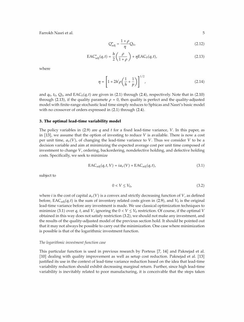
Farrokh Nasri et al. 5

Q∗adj =

1 + ρ

ηQ0, (2.12)

EAC∗adj(q, t) =

h

2

(ρ

1 + ρ

)+ ηEAC0(q, t), (2.13)

where

η =

[1 + 2h′ρ

(1h+1p

)]1/2

, (2.14)

and q0, t0, Q0, and EAC0(q, t) are given in (2.1) through (2.4), respectively. Note that in (2.10)through (2.13), if the quality paramete ρ = 0, then quality is perfect and the quality-adjustedmodel with finite-range stochastic lead time simply reduces to Sphicas and Nasri’s basic modelwith no crossover of orders expressed in (2.1) through (2.4).

3. The optimal lead-time variability model

The policy variables in (2.9) are q and t for a fixed lead-time variance, V . In this paper, asin [13], we assume that the option of investing to reduce V is available. There is now a costper unit time, av(V ), of changing the lead-time variance to V . Thus we consider V to be adecision variable and aim at minimizing the expected average cost per unit time composed ofinvestment to change V , ordering, backordering, nondefective holding, and defective holdingcosts. Specifically, we seek to minimize

EACadj(q, t, V ) = iav(V ) + EACadj(q, t), (3.1)

subject to

0 < V ≤ V0, (3.2)

where i is the cost of capital av(V ) is a convex and strictly decreasing function of V , as definedbefore, EACadj(q, t) is the sum of inventory related costs given in (2.9), and V0 is the originallead-time variance before any investment is made. We use classical optimization techniques tominimize (3.1) over q, t, and V , ignoring the 0 < V ≤ V0 restriction. Of course, if the optimal Vobtained in this way does not satisfy restriction (3.2), we should not make any investment, andthe results of the quality-adjusted model of the previous section hold. It should be pointed outthat it may not always be possible to carry out the minimization. One case where minimizationis possible is that of the logarithmic investment function.

The logarithmic investment function case

This particular function is used in previous research by Porteus [7, 14] and Paknejad et al.[10] dealing with quality improvement as well as setup cost reduction. Paknejad et al. [13]justified its use in the context of lead-time variance reduction based on the idea that lead-timevariability reduction should exhibit decreasing marginal return. Further, since high lead-timevariability is inevitably related to poor manufacturing, it is conceivable that the steps taken

6 Journal of Applied Mathematics and Decision Sciences

to improve the manufacturing process through improved quality and reduced setup time areclosely analogous to that of lead-time variability reduction. In this case, lead-time variancedeclines exponentially as the investment amount av increases. That is,

av(V ) =1ΓlnV0

Vfor 0 < V ≤ V0, (3.3)

where Γ is the percentage decrease in V per dollar increase in av. Here, our main objective is tominimize EACadj(q, t, V ) after substituting (3.3) and (2.9) into (3.1).

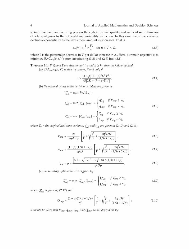
Theorem 3.1. If V0 and Γ are strictly positive and k ≥ k2, then the following hold:(a) EACadj(q, t, V ) is strictly convex, if and only if

q >(1 + ρ)(h + p)2D2V 2Γ4i[2K + (h + p)DV

] ; (3.4)

(b) the optimal values of the decision variables are given by

V ∗adj = min{V0, Vimp},

q∗∗adj = min{q∗adj, qimp} =

⎧⎨⎩q∗adj if Vimp ≥ V0,

qimp if Vimp < V0,

t∗∗adj = max{t∗adj, timp} =

⎧⎨⎩t∗adj if Vimp ≥ V0,

timp if Vimp < V0,

(3.5)

where V0 = the original lead-time variance, q∗adj and t∗adj are given in (2.10) and (2.11),

Vimp =2i

ΓhpD2η2

⎡⎣ i

Γ+

√i2

Γ2+

2η2DK

(1/h + 1/p)

⎤⎦ , (3.6)

qimp =(1 + ρ)(1/h + 1/p)

η2D

⎡⎣ i

Γ+

√i2

Γ2+

2η2DK

(1/h + 1/p)

⎤⎦ , (3.7)

timp = μ −

[i/Γ +

√i2/Γ2 + 2η2DK/(1/h + 1/p)

]η2Dp

; (3.8)

(c) the resulting optimal lot size is given by

Q∗∗adj = min{Q∗

adj, Qimp} =

⎧⎨⎩Q∗

adj if Vimp ≥ V0,

Qimp if Vimp < V0,(3.9)

where Q∗adj is given by (2.12) and

Qimp =(1 + ρ)(1/h + 1/p)

η2

⎡⎣ i

Γ+

√i2

Γ2+

2η2DK

(1/h + 1/p)

⎤⎦ ; (3.10)

it should be noted that Vimp, qimp, timp, and Qimp do not depend on V0;

Farrokh Nasri et al. 7

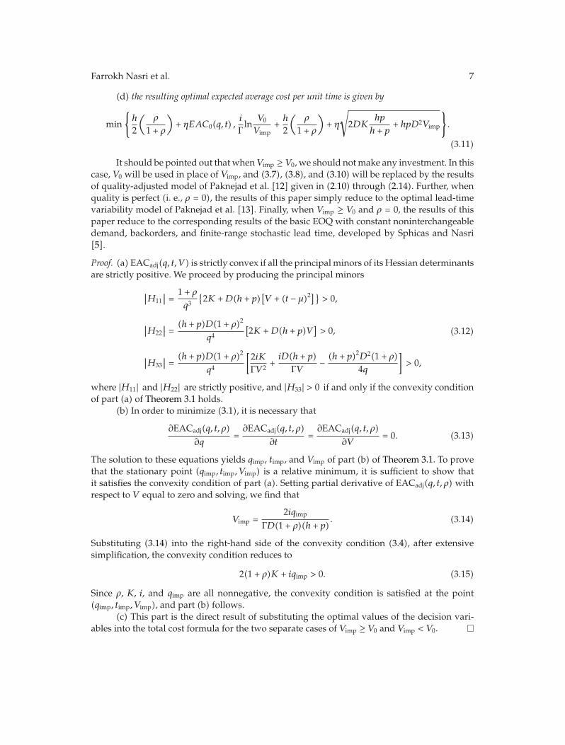
(d) the resulting optimal expected average cost per unit time is given by

min

{h

2

(ρ

1 + ρ

)+ ηEAC0(q, t) ,

i

Γln

V0

Vimp+h

2

(ρ

1 + ρ

)+ η

√2DK

hp

h + p+ hpD2Vimp

}.

(3.11)

It should be pointed out that when Vimp ≥ V0, we should notmake any investment. In thiscase, V0 will be used in place of Vimp, and (3.7), (3.8), and (3.10)will be replaced by the resultsof quality-adjusted model of Paknejad et al. [12] given in (2.10) through (2.14). Further, whenquality is perfect (i. e., ρ = 0), the results of this paper simply reduce to the optimal lead-timevariability model of Paknejad et al. [13]. Finally, when Vimp ≥ V0 and ρ = 0, the results of thispaper reduce to the corresponding results of the basic EOQ with constant noninterchangeabledemand, backorders, and finite-range stochastic lead time, developed by Sphicas and Nasri[5].

Proof. (a) EACadj(q, t, V ) is strictly convex if all the principal minors of its Hessian determinantsare strictly positive. We proceed by producing the principal minors

∣∣H11∣∣ = 1 + ρ

q3{2K +D(h + p)

[V + (t − μ)2

]}> 0,

∣∣H22∣∣ = (h + p)D(1 + ρ)2

q4[2K +D(h + p)V

]> 0,

∣∣H33∣∣ = (h + p)D(1 + ρ)2

q4

[2iKΓV 2

+iD(h + p)

ΓV− (h + p)2D2(1 + ρ)

4q

]> 0,

(3.12)

where |H11| and |H22| are strictly positive, and |H33| > 0 if and only if the convexity conditionof part (a) of Theorem 3.1 holds.

(b) In order to minimize (3.1), it is necessary that

∂EACadj(q, t, ρ)∂q

=∂EACadj(q, t, ρ)

∂t=∂EACadj(q, t, ρ)

∂V= 0. (3.13)

The solution to these equations yields qimp, timp, and Vimp of part (b) of Theorem 3.1. To provethat the stationary point (qimp, timp, Vimp) is a relative minimum, it is sufficient to show thatit satisfies the convexity condition of part (a). Setting partial derivative of EACadj(q, t, ρ) withrespect to V equal to zero and solving, we find that

Vimp =2iqimp

ΓD(1 + ρ)(h + p). (3.14)

Substituting (3.14) into the right-hand side of the convexity condition (3.4), after extensivesimplification, the convexity condition reduces to

2(1 + ρ)K + iqimp > 0. (3.15)

Since ρ, K, i, and qimp are all nonnegative, the convexity condition is satisfied at the point(qimp, timp, Vimp), and part (b) follows.

(c) This part is the direct result of substituting the optimal values of the decision vari-ables into the total cost formula for the two separate cases of Vimp ≥ V0 and Vimp < V0.

8 Journal of Applied Mathematics and Decision Sciences

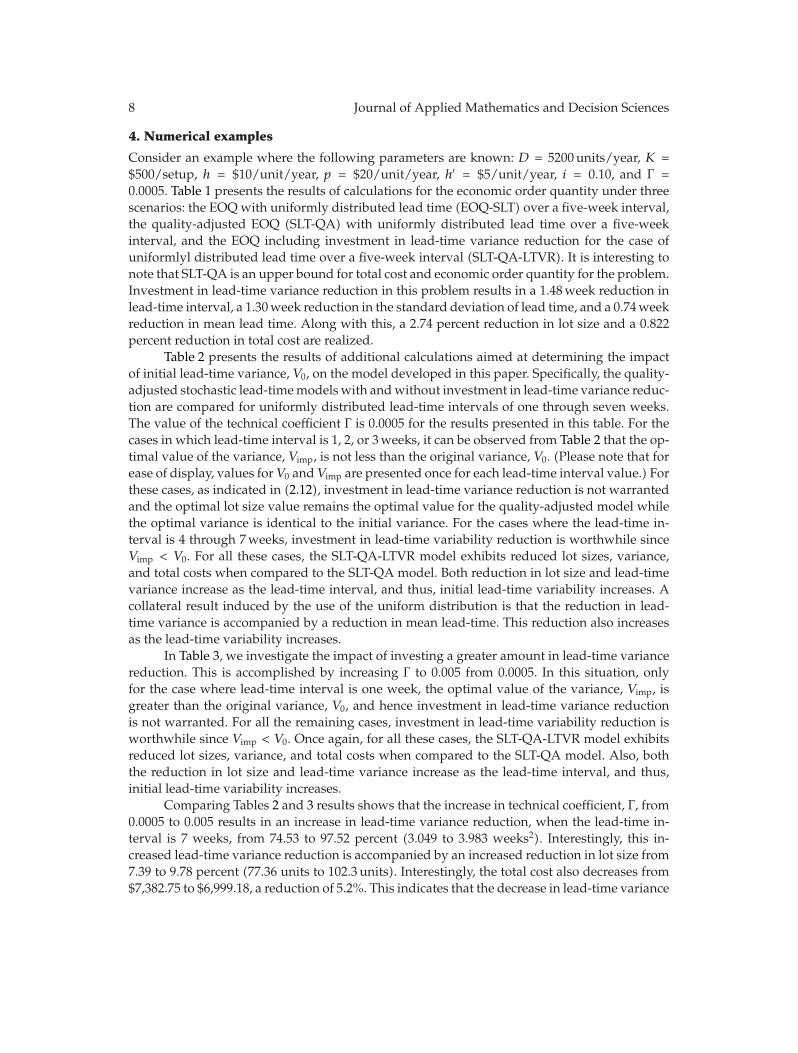
4. Numerical examples

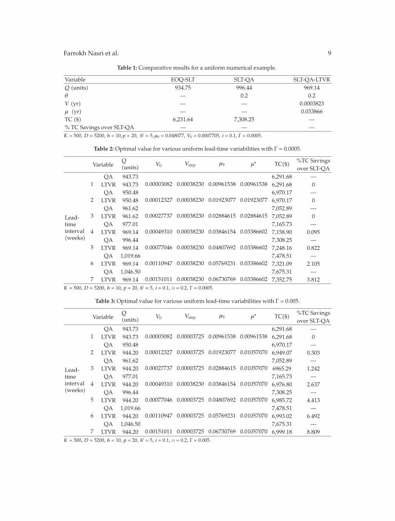
Consider an example where the following parameters are known: D = 5200 units/year, K =$500/setup, h = $10/unit/year, p = $20/unit/year, h′ = $5/unit/year, i = 0.10, and Γ =0.0005. Table 1 presents the results of calculations for the economic order quantity under threescenarios: the EOQwith uniformly distributed lead time (EOQ-SLT) over a five-week interval,the quality-adjusted EOQ (SLT-QA) with uniformly distributed lead time over a five-weekinterval, and the EOQ including investment in lead-time variance reduction for the case ofuniformlyl distributed lead time over a five-week interval (SLT-QA-LTVR). It is interesting tonote that SLT-QA is an upper bound for total cost and economic order quantity for the problem.Investment in lead-time variance reduction in this problem results in a 1.48week reduction inlead-time interval, a 1.30week reduction in the standard deviation of lead time, and a 0.74weekreduction in mean lead time. Along with this, a 2.74 percent reduction in lot size and a 0.822percent reduction in total cost are realized.

Table 2 presents the results of additional calculations aimed at determining the impactof initial lead-time variance, V0, on the model developed in this paper. Specifically, the quality-adjusted stochastic lead-timemodels with andwithout investment in lead-time variance reduc-tion are compared for uniformly distributed lead-time intervals of one through seven weeks.The value of the technical coefficient Γ is 0.0005 for the results presented in this table. For thecases in which lead-time interval is 1, 2, or 3weeks, it can be observed from Table 2 that the op-timal value of the variance, Vimp, is not less than the original variance, V0. (Please note that forease of display, values for V0 and Vimp are presented once for each lead-time interval value.) Forthese cases, as indicated in (2.12), investment in lead-time variance reduction is not warrantedand the optimal lot size value remains the optimal value for the quality-adjusted model whilethe optimal variance is identical to the initial variance. For the cases where the lead-time in-terval is 4 through 7weeks, investment in lead-time variability reduction is worthwhile sinceVimp < V0. For all these cases, the SLT-QA-LTVR model exhibits reduced lot sizes, variance,and total costs when compared to the SLT-QA model. Both reduction in lot size and lead-timevariance increase as the lead-time interval, and thus, initial lead-time variability increases. Acollateral result induced by the use of the uniform distribution is that the reduction in lead-time variance is accompanied by a reduction in mean lead-time. This reduction also increasesas the lead-time variability increases.

In Table 3, we investigate the impact of investing a greater amount in lead-time variancereduction. This is accomplished by increasing Γ to 0.005 from 0.0005. In this situation, onlyfor the case where lead-time interval is one week, the optimal value of the variance, Vimp, isgreater than the original variance, V0, and hence investment in lead-time variance reductionis not warranted. For all the remaining cases, investment in lead-time variability reduction isworthwhile since Vimp < V0. Once again, for all these cases, the SLT-QA-LTVR model exhibitsreduced lot sizes, variance, and total costs when compared to the SLT-QA model. Also, boththe reduction in lot size and lead-time variance increase as the lead-time interval, and thus,initial lead-time variability increases.

Comparing Tables 2 and 3 results shows that the increase in technical coefficient, Γ, from0.0005 to 0.005 results in an increase in lead-time variance reduction, when the lead-time in-terval is 7 weeks, from 74.53 to 97.52 percent (3.049 to 3.983 weeks2). Interestingly, this in-creased lead-time variance reduction is accompanied by an increased reduction in lot size from7.39 to 9.78 percent (77.36 units to 102.3 units). Interestingly, the total cost also decreases from$7,382.75 to $6,999.18, a reduction of 5.2%. This indicates that the decrease in lead-time variance

Farrokh Nasri et al. 9

Table 1: Comparative results for a uniform numerical example.

Variable EOQ-SLT SLT-QA SLT-QA-LTVRQ (units) 934.75 996.44 969.14θ — 0.2 0.2V (yr) — — 0.0003823μ (yr) — — 0.033866TC ($) 6,231.64 7,308.25 —% TC Savings over SLT-QA — — —K = 500, D = 5200, h = 10, p = 20, h′ = 5, μ0 = 0.048077, V0 = 0.0007705, i = 0.1, Γ = 0.0005.

Table 2: Optimal value for various uniform lead-time variabilities with Γ = 0.0005.

VariableQ(units) V0 Vimp μ0 μ∗ TC($)

%TC Savingsover SLT-QA

Lead-timeinterval(weeks)

1QA 943.73

0.00003082 0.00038230 0.00961538 0.009615386,291.68 —

LTVR 943.73 6,291.68 0

2QA 950.48

0.00012327 0.00038230 0.01923077 0.019230776,970.17 —

LTVR 950.48 6,970.17 0

3QA 961.62

0.00027737 0.00038230 0.02884615 0.028846157,052.89 —

LTVR 961.62 7,052.89 0

4QA 977.01

0.00049310 0.00038230 0.03846154 0.033866027,165.73 —

LTVR 969.14 7,158.90 0.095

5QA 996.44

0.00077046 0.00038230 0.04807692 0.033866027,308.25 —

LTVR 969.14 7,248.16 0.822

6QA 1,019.66

0.00110947 0.00038230 0.05769231 0.033866027,478.51 —

LTVR 969.14 7,321.09 2.105

7QA 1,046.50

0.00151011 0.00038230 0.06730769 0.033866027,675.31 —

LTVR 969.14 7,352.75 3.812K = 500, D = 5200, h = 10, p = 20, h′ = 5, i = 0.1, � = 0.2, Γ = 0.0005.

Table 3: Optimal value for various uniform lead-time variabilities with Γ = 0.005.

VariableQ(units) V0 Vimp μ0 μ∗ TC($)

%TC Savingsover SLT-QA

Lead-timeinterval(weeks)

1QA 943.73

0.00003082 0.00003725 0.00961538 0.009615386,291.68 —

LTVR 943.73 6,291.68 0

2QA 950.48

0.00012327 0.00003725 0.01923077 0.010570706,970.17 —

LTVR 944.20 6,949.07 0.303

3QA 961.62

0.00027737 0.00003725 0.02884615 0.010570707,052.89 —

LTVR 944.20 6965.29 1.242

4QA 977.01

0.00049310 0.00038230 0.03846154 0.010570707,165.73 —

LTVR 944.20 6,976.80 2.637

5QA 996.44

0.00077046 0.00003725 0.04807692 0.010570707,308.25 —

LTVR 944.20 6,985.72 4.413

6QA 1,019.66

0.00110947 0.00003725 0.05769231 0.010570707,478.51 —

LTVR 944.20 6,993.02 6.492

7QA 1,046.50

0.00151011 0.00003725 0.06730769 0.010570707,675.31 —

LTVR 944.20 6,999.18 8.809K = 500, D = 5200, h = 10, p = 20, h′ = 5, i = 0.1, � = 0.2, Γ = 0.005.

10 Journal of Applied Mathematics and Decision Sciences

Table 4: Optimal value for various normal lead-time variabilities.

Lead-time interval (weeks)

Variable1 2 3 4 5

QA LTVR QA Imp QA Imp QA Imp QA Imp

Q (units) 942.73 942.23 944.48 944.20 948.23 944.20 953.46 944.20 960.44 944.20V0 0.00001027 0.00004109 0.00009246 0.00016437 0.00025682Vimp 0.00003725 0.00003725 0.00003725 0.00003725 0.00003725TC($) 6,910.64 6,910.64 6,927.20 6,927.09 6,954.72 6,943.32 6,993.06 6,954.82 7,041.05 6,963.75

% TC

— 0 — 0.159 — 0.164 — 0.976 — 1.098SavingsoverSLT-QAK = 500, D = 5200, h = 10, p = 20, h′ = 5, i = 0.1, � = 0.2, Γ = 0.005.

Table 5: Optimal values for various values of �.Variable Q Vimp μ∗ TC ($)

�

0.025 891.86 0.00004288 0.01134166 6,091.39

0.050 897.93 0.00004206 0.01123338 6,208.250.075 904.43 0.00004125 0.01112462 6,330.000.100 911.38 0.00004045 0.01101530 6,456.870.125 918.79 0.00003964 0.01090535 6,589.080.150 926.71 0.00003884 0.01079466 6,726.900.175 935.17 0.00003804 0.01068314 6,870.640.200 944.20 0.00003725 0.01057069 7,020.650.225 953.84 0.00003645 0.01045722 7,177.320.250 964.15 0.00003566 0.01034260 7,341.110.275 975.17 0.00003486 0.01022671 7,512.520.300 986.96 0.00003407 0.01010941 7,692.15

K = 500, D = 5200, h = 10, p = 20, h′ = 5, i = 0.1, LT Interval = 7weeks, Γ = 0.005.

along with the resulting synergistic impact on the lot size clearly improves the overall perfor-mance of the production and inventory system.

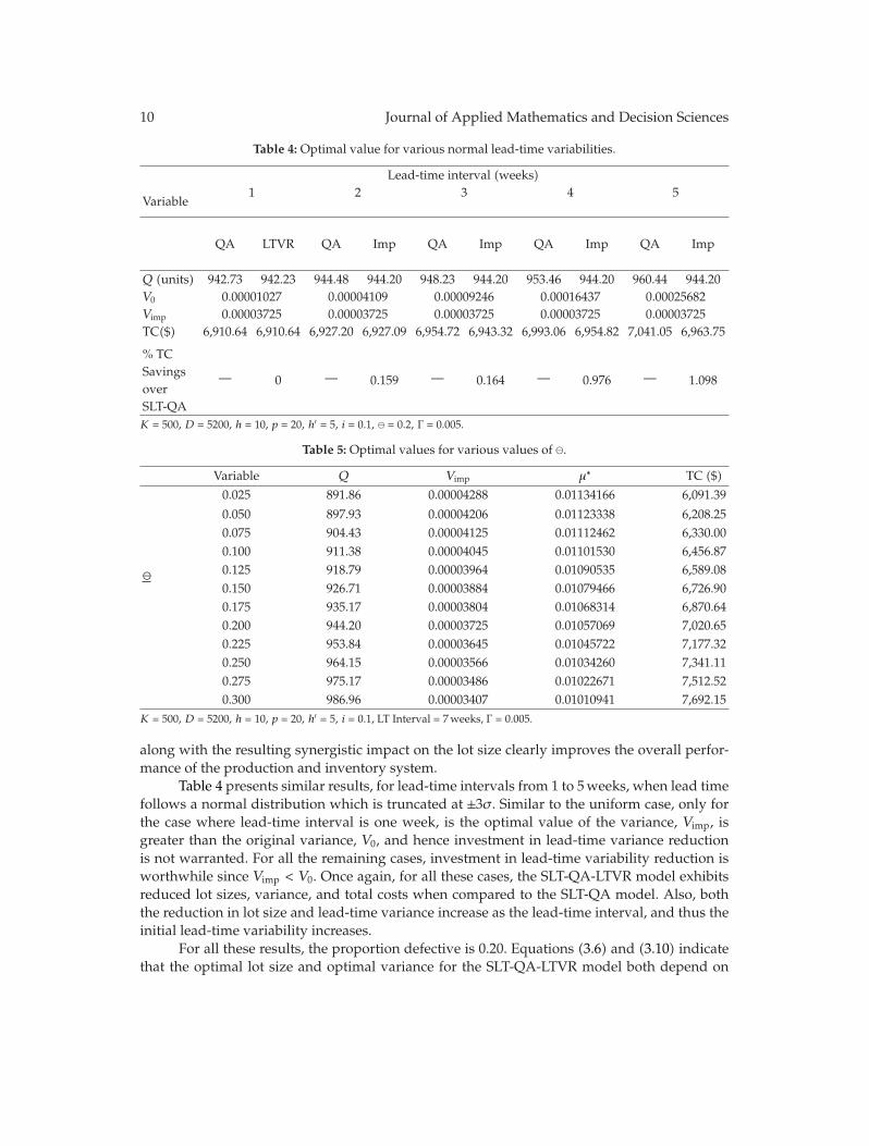
Table 4 presents similar results, for lead-time intervals from 1 to 5weeks, when lead timefollows a normal distribution which is truncated at ±3σ. Similar to the uniform case, only forthe case where lead-time interval is one week, is the optimal value of the variance, Vimp, isgreater than the original variance, V0, and hence investment in lead-time variance reductionis not warranted. For all the remaining cases, investment in lead-time variability reduction isworthwhile since Vimp < V0. Once again, for all these cases, the SLT-QA-LTVR model exhibitsreduced lot sizes, variance, and total costs when compared to the SLT-QA model. Also, boththe reduction in lot size and lead-time variance increase as the lead-time interval, and thus theinitial lead-time variability increases.

For all these results, the proportion defective is 0.20. Equations (3.6) and (3.10) indicatethat the optimal lot size and optimal variance for the SLT-QA-LTVR model both depend on

Farrokh Nasri et al. 11

the proportion defective, θ. Therefore, a logical question to ask is exactly what is the impact ofthis parameter? Table 5 presents results for defect proportion values from 0.025 to 0.30 for thesituation where lead-time follows a uniform distribution with a 7-week lead-time interval andthe technical parameter Γ = 0.005. Note that a lead-time variance reduction on the order of 97%is realized in all cases. There is slightly less of an impact of lead-time variance reduction for asmaller-proportions defective. We also observe a decrease in lot size as the proportion defec-tive decreases. On a relative basis, this decrease is on the order of 5.2 percent when comparedto the lot size generated by the solution to the SLT-QA model, increasing slightly on a per-centage basis as θ increases. The total inventory-related cost of implementing SLT-QA-LTVRdecreases significantly as the proportion defective decreases. These results provide some pre-liminary evidence for the concept that programs directed at simultaneously improving qual-ity, and reducing lead-time variability will have a synergistic impact on the performance ofproduction-inventory systems.

5. Sensitivity analysis

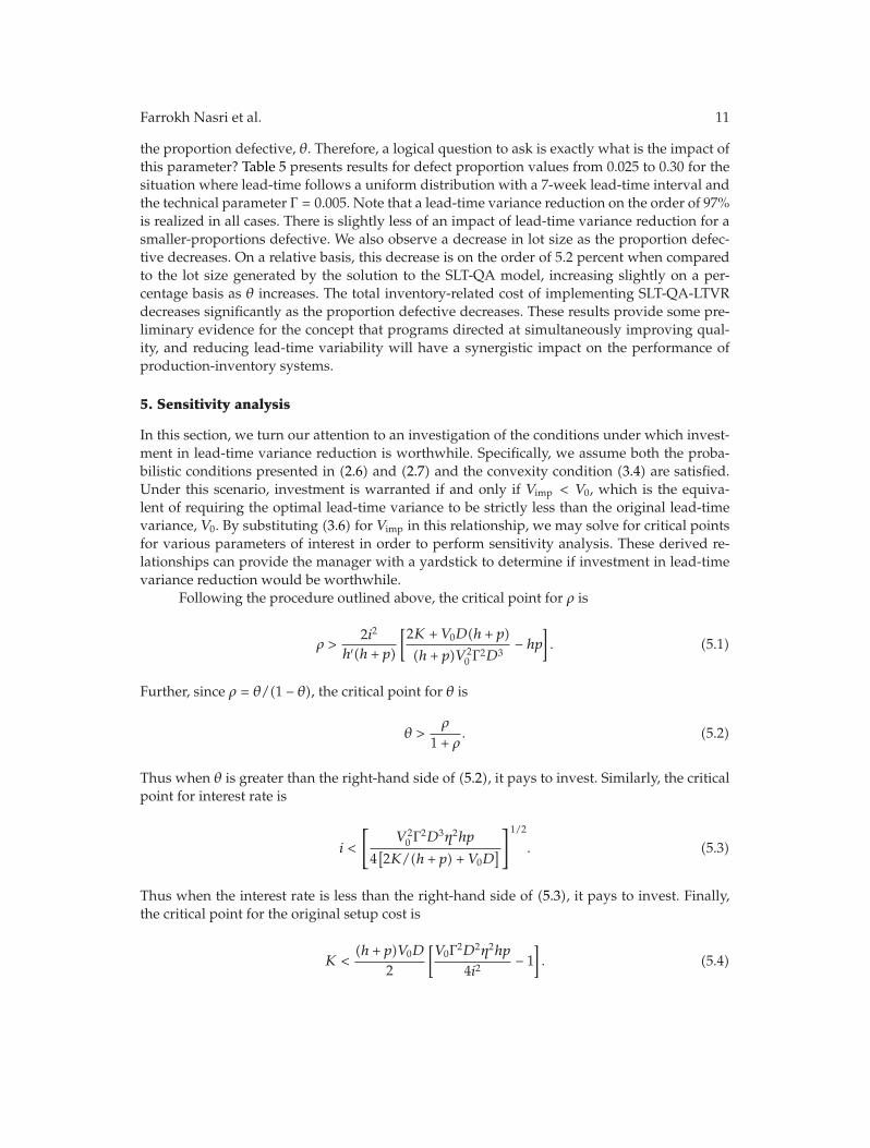
In this section, we turn our attention to an investigation of the conditions under which invest-ment in lead-time variance reduction is worthwhile. Specifically, we assume both the proba-bilistic conditions presented in (2.6) and (2.7) and the convexity condition (3.4) are satisfied.Under this scenario, investment is warranted if and only if Vimp < V0, which is the equiva-lent of requiring the optimal lead-time variance to be strictly less than the original lead-timevariance, V0. By substituting (3.6) for Vimp in this relationship, we may solve for critical pointsfor various parameters of interest in order to perform sensitivity analysis. These derived re-lationships can provide the manager with a yardstick to determine if investment in lead-timevariance reduction would be worthwhile.

Following the procedure outlined above, the critical point for ρ is

ρ >2i2

h′(h + p)

[2K + V0D(h + p)

(h + p)V 20 Γ

2D3− hp

]. (5.1)

Further, since ρ = θ/(1 − θ), the critical point for θ is

θ >ρ

1 + ρ. (5.2)

Thus when θ is greater than the right-hand side of (5.2), it pays to invest. Similarly, the criticalpoint for interest rate is

i <

[V 20 Γ

2D3η2hp

4[2K/(h + p) + V0D

]]1/2

. (5.3)

Thus when the interest rate is less than the right-hand side of (5.3), it pays to invest. Finally,the critical point for the original setup cost is

K <(h + p)V0D

2

[V0Γ2D2η2hp

4i2− 1

]. (5.4)

12 Journal of Applied Mathematics and Decision Sciences

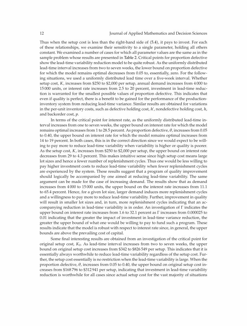
Thus when the setup cost is less than the right-hand side of (5.4), it pays to invest. For eachof these relationships, we examine their sensitivity to a single parameter, holding all othersconstant. We examined a number of cases for which all parameter values are the same as in thesample problem whose results are presented in Table 2. Critical points for proportion defectiveshow the lead-time variability reductionmodel to be quite robust. As the uniformly distributedlead-time interval increases from two to seven weeks, the lower bound on proportion defectivefor which the model remains optimal decreases from 0.05 to, essentially, zero. For the follow-ing situations, we used a uniformly distributed lead time over a five-week interval. Whethersetup cost, K, increases from $250 to $2,000 per setup, annual demand increases from 4 000 to15 000 units, or interest rate increases from 2.5 to 20 percent, investment in lead-time reduc-tion is warranted for the smallest possible values of proportion defective. This indicates thateven if quality is perfect, there is a benefit to be gained for the performance of the production-inventory system from reducing lead-time variance. Similar results are obtained for variationsin the per-unit inventory costs, such as defective holding cost, h′, nondefective holding cost, h,and backorder cost, p.

In terms of the critical point for interest rate, as the uniformly distributed lead-time in-terval increases from one to seven weeks, the upper bound on interest rate for which the modelremains optimal increases from 1 to 28.5 percent. As proportion defective, θ, increases from 0.05to 0.40, the upper bound on interest rate for which the model remains optimal increases from14 to 19 percent. In both cases, this is in the correct direction since we would expect to be will-ing to pay more to reduce lead-time variability when variability is higher or quality is poorer.As the setup cost, K, increases from $250 to $2,000 per setup, the upper bound on interest ratedecreases from 29 to 4.3 percent. This makes intuitive sense since high setup cost means largelot sizes and hence a fewer number of replenishment cycles. Thus one would be less willing topay higher investment costs to reduce lead-time variability when fewer replenishment cyclesare experienced by the system. These results suggest that a program of quality improvementshould logically be accompanied by one aimed at reducing lead-time variability. The sameargument can be made for the case of increasing demand. The results show that as demandincreases from 4 000 to 15 000 units, the upper bound on the interest rate increases from 11.1to 65.4 percent. Hence, for a given lot size, larger demand induces more replenishment cyclesand a willingness to pay more to reduce lead-time variability. Further, improvement in qualitywill result in smaller lot sizes and, in turn, more replenishment cycles indicating that an ac-companying reduction in lead-time variability is in order. An investigation of Γ indicates theupper bound on interest rate increases from 1.6 to 32.1 percent as Γ increases from 0.000025 to0.01 indicating that the greater the impact of investment in lead-time variance reduction, thegreater the upper bound of what one would be willing to pay to fund such a program. Theseresults indicate that the model is robust with respect to interest rate since, in general, the upperbounds are above the prevailing cost of capital.

Some final interesting results are obtained from an investigation of the critical point fororiginal setup cost, K0. As lead-time interval increases from two to seven weeks, the upperbound on original setup cost increases from $342 to $826 549 per setup. This indicates that it isessentially always worthwhile to reduce lead-time variability regardless of the setup cost. Fur-ther, the setup cost essentially is no restriction when the lead-time variability is large. When theproportion defective, θ, increases from 0.05 to 0.40, the upper bound on original setup cost in-creases from $168 796 to $312 941 per setup, indicating that investment in lead-time variabilityreduction is worthwhile for all cases since actual setup cost for the vast majority of situations

Farrokh Nasri et al. 13

are lower than the upper bound. These results indicate that there is certainly significant roomfor reducing setup costs and lead-time variability while simultaneously engaging in a programof quality improvement.

6. Conclusion

This paper presents an extension of the quality-adjusted EOQmodel with finite-range stochas-tic lead-times in which investment in lead-time variance reduction is considered. Specifically, aquality-adjusted lead-time variance reduction model is developed in which the lead-time vari-ance is treated as a decision variable. This model assumes investment in lead-time variance re-duction proceeds according to a logarithmic investment function. Relationships for economiclot size, optimal total cost, optimal number of time units of demand satisfied by each order,and the optimal time differential between placing an order and the start of q time units thatwill be satisfied by the given order, as well as optimal lead-time variance, are derived. Resultsof numerical examples indicate that savings can be realized by investing in lead-time variancereduction. The results of sensitivity analysis relating to proportion defective, interest rate, andsetup cost show the lead-time variance reduction model to be quite robust and representativeof practice.

References

[1] D. Gross and A. Soriano, “The effect of reducing lead time on inventory level-simulation analysis,”Management Science, vol. 16, pp. B61–B76, 1969.

[2] C. E. Vinson, “The cost of ignoring lead time unreliability in inventory theory,”Decision Sciences, vol. 3,no. 2, pp. 87–105, 1972.

[3] M. J. Liberatore, “The EOQ model under stochastic lead time,” Operations Research, vol. 27, no. 2, pp.391–396, 1979.

[4] G. P. Sphicas, “On the solution of an inventory model with variable lead times,” Operations Research,vol. 30, no. 2, pp. 404–410, 1982.

[5] G. P. Sphicas and F. Nasri, “An inventorymodel with finite-range stochastic lead times,”Naval ResearchLogistics Quarterly, vol. 31, no. 4, pp. 609–616, 1984.

[6] M. J. Rosenblatt and H. L. Lee, “Economic production cycles with imperfect production processes,”IIE Transactions, vol. 18, no. 1, pp. 48–55, 1986.

[7] E. L. Porteus, “Optimal lot sizing, process quality improvement and setup cost reduction,” OperationsResearch, vol. 34, no. 1, pp. 137–144, 1986.

[8] T. C. E. Cheng, “EPQ with process capability and quality assurance considerations,” Journal of Opera-tional Research Society, vol. 42, no. 8, pp. 713–720, 1991.

[9] K.Moinzadeh and H. L. Lee, “A continuous-review inventory model with constant resupply time anddefective items,” Naval Research Logistics, vol. 34, no. 4, pp. 457–467, 1987.

[10] M. J. Paknejad, F. Nasri, and J. F. Affisco, “Defective units in a continuous review (s,Q) system,”International Journal of Production Research, vol. 33, no. 10, pp. 2767–2777, 1995.

[11] E. Heard and G. Plossl, “Lead times revisited,” Production and Inventory Management, vol. 23, no. 3, pp.32–47, 1984.

[12] J. Paknejad, F. Nasri, and J. F. Affisco, “Quality improvement in an inventory model with finite-rangestochastic lead times,” Journal of Applied Mathematics and Decision Sciences, vol. 2005, no. 3, pp. 177–189,2005.

[13] M. J. Paknejad, F. Nasri, and J. F. Affisco, “Lead-time variability reduction in stochastic inventorymodels,” European Joural of Operational Research, vol. 62, no. 3, pp. 311–322, 1992.

[14] E. L. Porteus, “Investing in new parameter values in the discounted EOQ model,” Naval ResearchLogistics Quarterly, vol. 33, no. 1, pp. 39–48, 1986.

Submit your manuscripts athttp://www.hindawi.com

Hindawi Publishing Corporationhttp://www.hindawi.com Volume 2014

MathematicsJournal of

Hindawi Publishing Corporationhttp://www.hindawi.com Volume 2014

Mathematical Problems in Engineering

Hindawi Publishing Corporationhttp://www.hindawi.com

Differential EquationsInternational Journal of

Volume 2014

Applied MathematicsJournal of

Hindawi Publishing Corporationhttp://www.hindawi.com Volume 2014

Probability and StatisticsHindawi Publishing Corporationhttp://www.hindawi.com Volume 2014

Journal of

Hindawi Publishing Corporationhttp://www.hindawi.com Volume 2014

Mathematical PhysicsAdvances in

Complex AnalysisJournal of

Hindawi Publishing Corporationhttp://www.hindawi.com Volume 2014

OptimizationJournal of

Hindawi Publishing Corporationhttp://www.hindawi.com Volume 2014

CombinatoricsHindawi Publishing Corporationhttp://www.hindawi.com Volume 2014

International Journal of

Hindawi Publishing Corporationhttp://www.hindawi.com Volume 2014

Operations ResearchAdvances in

Journal of

Hindawi Publishing Corporationhttp://www.hindawi.com Volume 2014

Function Spaces

Abstract and Applied AnalysisHindawi Publishing Corporationhttp://www.hindawi.com Volume 2014

International Journal of Mathematics and Mathematical Sciences

Hindawi Publishing Corporationhttp://www.hindawi.com Volume 2014

The Scientific World JournalHindawi Publishing Corporation http://www.hindawi.com Volume 2014

Hindawi Publishing Corporationhttp://www.hindawi.com Volume 2014

Algebra

Discrete Dynamics in Nature and Society

Hindawi Publishing Corporationhttp://www.hindawi.com Volume 2014

Hindawi Publishing Corporationhttp://www.hindawi.com Volume 2014

Decision SciencesAdvances in

Discrete MathematicsJournal of

Hindawi Publishing Corporationhttp://www.hindawi.com

Volume 2014 Hindawi Publishing Corporationhttp://www.hindawi.com Volume 2014

Stochastic AnalysisInternational Journal of