
Investigation on Smoke Movement and Smoke Control for ...
124
Investigation on Smoke Movement and Smoke Control for Atrium in Green and Sustainable Buildings Liu Fang Peter V. Nielsen Henrik Brohus Department of Civil Engineering ISSN 1901-726X DCE Technical Report No. 32
Transcript of Investigation on Smoke Movement and Smoke Control for ...

Investigation on Smoke Movementand Smoke Control for Atrium inGreen and Sustainable Buildings
Liu FangPeter V. Nielsen
Henrik Brohus
Department of Civil EngineeringISSN 1901-726X DCE Technical Report No. 32
DCE Technical Report No. 32
Aalborg University Department of Civil Engineering
Investigation on Smoke Movement and Smoke Control for Atrium in Green and Sustainable
Buildings
by
Liu Fang Peter V. Nielsen Henrik Brohus
June 2007
© Aalborg University

Scientific Publications at the Department of Civil Engineering Technical Reports are published for timely dissemination of research results and scientific workcarried out at the Department of Civil Engineering (DCE) at Aalborg University. This mediumallows publication of more detailed explanations and results than typically allowed in scientificjournals. Technical Memoranda are produced to enable the preliminary dissemination of scientific work by the personnel of the DCE where such release is deemed to be appropriate. Documents of this kindmay be incomplete or temporary versions of papers—or part of continuing work. This should be kept in mind when references are given to publications of this kind. Contract Reports are produced to report scientific work carried out under contract. Publications ofthis kind contain confidential matter and are reserved for the sponsors and the DCE. Therefore,Contract Reports are generally not available for public circulation. Lecture Notes contain material produced by the lecturers at the DCE for educational purposes. Thismay be scientific notes, lecture books, example problems or manuals for laboratory work, orcomputer programs developed at the DCE. Theses are monograms or collections of papers published to report the scientific work carried out atthe DCE to obtain a degree as either PhD or Doctor of Technology. The thesis is publicly availableafter the defence of the degree. Latest News is published to enable rapid communication of information about scientific workcarried out at the DCE. This includes the status of research projects, developments in thelaboratories, information about collaborative work and recent research results.
Published 2007 by Aalborg University Department of Civil Engineering Sohngaardsholmsvej 57, DK-9000 Aalborg, Denmark Printed in Aalborg at Aalborg University ISSN 1901-726X DCE Technical Report No. 32

Investigation on Smoke Movement and Smoke Control for
Atrium in Green and Sustainable Buildings
Supported by European Community Asia-link Project
Centre of Sino-European Sustainable Building Design & Construction
(Contract No.: CN/ASIA-LINK/011(91-400))
by
Liu Fang
June 2007
A report submitted in partial fulfillment of the requirements for European Community Asia-link Project
Department of Civil Engineering Aalborg University
Sohngaardsholmsvej 57 DK-9000 Aalborg, Denmark

Acknowledgements
I
Acknowledgements
This research was carried out by the support of European Community Asia-link Project
(Contract No.: CN/ASIA-LINK/011(91-400)). The experiments were conducted in the
laboratory of civil engineering department of Aalborg University.
I would like to thank the following people and organization who have contributed to
this research in various ways:
Thanks to Per Heiselberg, R.M. Yao and B.Z. Li for providing me to work in Aalborg
University Denmark and their care during my stay in Aalborg.
Thanks to Per Heiselberg for his instruction on ventilation course. Thanks to P.V.
Nielsen for his instruction on similarity theory and the design of the experimental
schemes. Their ideas broadened my knowledge and fuelled my enthusiasm to carry out
the research.
Thanks to Heidi Stentoft and Torben Christensen for their help with experiment.
Thanks to Rasmus Lund Jensen for his help in FDS simulation. Thanks to Henrik
Brohus and Carl-Erik Hyldgård for their help.
Thanks to P.V. Nielsen, Bente J. Kjærgaard and Zhigang Li, for their invaluable help
with work and life in Aalborg.
Centre of Sino-European Sustainable Building Design & Construction, for providing
funding for this research.
Aalborg University, for providing me apartment and office.
Chongqing University, for supporting me.
Abstract
II
Abstract
The concepts of green buildings and sustainable buildings are promoted actively in the
developed countries. Targets are on protecting the environment, using less energy
through natural ventilation provisions and daylight utilization, developing better waste
management and taking resource conservation into account. Architectural and building
design, electrical and mechanical systems, and building management have to be
upgraded. However, there are problems in dealing with fire safety, especially in
complying with the existing prescriptive fire codes. A hot argument is that smoke
control system design in the green or sustainable buildings with an atrium.
Since the physics of air entrainment is not yet clearly understood, most of the fire plume
expressions reported in the literature was derived empirically. Experiments and CFD
simulation were used to study the different types of thermal plumes such as
axisymmetric plume, wall plume, corner plume and balcony spill plume in this report.
As many large space buildings such as cinema, sports arenas containing the sloping
floor are designed to meet the function and aesthetic requirement. The smoke
movement in atrium with sloping floor is also discussed in this report.
Computational Fluid Dynamics and scale model experiments are two possible methods
for the determination of mass transport, contaminant transport, smoke movement and
energy transport in large building. The scale model experiments and FDS (Fire
Dynamic Simulation) are used in this report.
Three axisymmetric plume equations and two balcony spill plume models are assessed
by comparing with the CFD and experiment results. Investigations in this report are
useful for fire engineers in designing smoke control systems.
This thesis also describes many significant atrium smoke movement and smoke
management research, related efforts and future research, the major topics are as
follows: types and configurations of atrium buildings; approach to atrium smoke
management design calculation in NFPA92B and comparison of two methods of
calculating smoke layer interface heights; smoke exhaust system modes and smoke

Abstract
III
exhaust effectiveness; atrium smoke filling process and its time constant;
pre-stratification and detection ; airflow for smoke control between the atrium and
communicating space; sprinkler effect, etc.
This report was written as a work report of my stay at the department of civil
engineering of Aalborg University from January 2007 to June 2007. As the time
limitation the further analysis of the result is needed when I go back to Chongqing
University.
Key Words
Sustainable building/ atrium/ smoke movement/ smoke control/ CFD/ scale model

Table of Contents
IV
Table of Contents
Acknowledgements ...............................................................................................................................I
Abstract ............................................................................................................................................... II
1 Introduction .......................................................................................................................................1
1.1 Background.....................................................................................................................................1
1.2 Types and Configurations ...............................................................................................................2
1.2.1 Atrium Type 1 Cubic ...................................................................................................................4
1.2.2 Atrium Type 2 Flat.......................................................................................................................4
1.2.3 Atrium Type 3 High.....................................................................................................................4
1.2.4 Atrium Fire Environment Simulation ..........................................................................................5
1.2.5 Atrium Types in Mainland China.................................................................................................5
1.3 Smoke Control................................................................................................................................7
1.3.1 Objectives for Smoke Control .....................................................................................................7
1.3.2 Smoke Control Systems...............................................................................................................7
1.3.3 Smoke and Heat Exhaust Ventilation Systems (Smoke Exhaust System) .................................10
1.4 Steady Smoke Layer Interface...................................................................................................... 11
1.4.1 Regular Ceiling Method ............................................................................................................ 11
1.4.2 Irregular Ceiling Method...........................................................................................................12
1.4.3 Comparison of Methods ............................................................................................................13
1.5 Smoke Exhaust Rate.....................................................................................................................14
1.5.1 Equation.....................................................................................................................................14
1.5.2 Discussion..................................................................................................................................15
1.6 Smoke Extraction System Modes and Smoke Exhaust Effectiveness..........................................17
1.7 Smoke Filling Processes and Time Constant................................................................................19
1.8 Airflow for Smoke Control between Atrium and Communicating Spaces...................................22
1.9 Sprinkler Effect.............................................................................................................................23
1.10 Research Objective.....................................................................................................................24
2 Governing Equations and Large Eddy Simulation ..........................................................................27
2.1 Governing Equation......................................................................................................................28
2.2 Turbulence Model.........................................................................................................................28
2.3 Sub Grid Scale Models.................................................................................................................30
2.4 FDS Introduction ..........................................................................................................................31
3 Similar Theory and Dimensionless Numbers ..................................................................................33
3.1 Similar Theory..............................................................................................................................33

Table of Contents
V
3.2 Similarity Principles and Conditions for Model Experiments......................................................36
4 Scale Model Experiment: Apparatus and Methodology..................................................................39
4.1 Physical Scale Model ...................................................................................................................39
4.2 Instrumentation.............................................................................................................................40
4.3 Test Methods.................................................................................................................................42
5 Experiment and FDS Simulation on Plume Entrainment for the Different Fire Location...............43
5.1 Experimental Conditions ..............................................................................................................44
5.2 Smoke Filling ...............................................................................................................................44
5.3 Center Fire (Fire A) ......................................................................................................................48
5.4 Wall Fire (Fire B)..........................................................................................................................51
5.5 Corner Fire (Fire C)......................................................................................................................53
5.6 Comparison...................................................................................................................................56
6 Experiment and FDS Simulation on Balcony Plume.......................................................................62
6.1 Smoke Movement from Atrium to Communicating Space...........................................................63
6.2 Smoke Movement from Communicating Space to Atrium...........................................................68
6.2.1 Experiment Result .....................................................................................................................68
6.2.2 FDS Simulation .........................................................................................................................71
6.3 Balcony Plume Entrainment.........................................................................................................76
7 Experiment and FDS Simulation on Smoke Movement in Large Space Building with Sloping
Floor ...................................................................................................................................................82
7.1 Experiment Condition...................................................................................................................84
7.2 Experimental Result of the Sloping Floor with Different Angle ..................................................85
7.3 Experimental Result of the Sloping Floor with 20 Degree...........................................................88
7.4 FDS Simulation ............................................................................................................................93
8 Conclusion.....................................................................................................................................100
Nomenclature ...................................................................................................................................101
References ........................................................................................................................................102
Appendix A.......................................................................................................................................105
Appendix B....................................................................................................................................... 110
Appendix C....................................................................................................................................... 113

1 Introduction
1
1 Introduction
1.1 Background
Over the last few decades, large undivided volume buildings such as atrium buildings,
covered shopping malls, airport terminals and sports arenas have become increasingly
popular. These buildings typically contain large spaces or voids which can occupy
many storey in height. The term ‘atrium’ can be applied to the large spaces within these
types of buildings.
The concept of an atrium dates back to Roman times, when used as an entrance hall in
a typical house. An atrium within a building is a large open space created by an
opening or series of opening in floor assemblies, thus connecting two or more stories
of a building that is closed at top. The sides of an atrium may be open to all floors, to
some of the floors or closed to all or some of the floors by unrated or rated
fire-resistant construction. As well, there may be two or more atria with in a single
building, all interconnected at the ground floor or on a number of floors.
Developments in architectural techniques now allow an atrium to be an integral part of
large buildings (e.g. covered shopping malls). Modern atria are designed with the
intention to provide a visually and spatially external environment in doors [1] [2].
In terms of fire protection, floors, ceilings and partitions are traditionally used to
provide space to limit the spread of fire and smoke within a building. However, atrium
buildings violate this fundamental approach in terms of horizontal space and vertical
separation. With a fire on the floor of an atrium or in any space open to it, smoke can
fill the atrium and connected floor spaces. The fire risks of atrium building are
different from those of traditional buildings, and the associated problems related to
smoke should be dealt with carefully.
‘Green buildings’ are of great interest to the developed countries towards the end of the
last century. Now, this is extended further to ‘sustainable buildings’ similar actions are
taken in big cities of China and Denmark. Although the concepts behind the two are
different, the assessment procedure is roughly the same. A ‘relative scale’ to a typical
building in a region will be applied for a green building. Sustainable building is more

1 Introduction
2
‘absolute’ on controlling energy and mass flows internationally. Indoor environment,
environmental protection, energy-saving through better provisions of natural
ventilation and utilization of daylight, water consumption and waste management are
the common approaches to satisfy the assessment criteria for those green or sustainable
buildings.
Normally, three items will be covered:
1) Architectural features including building construction element.
2) Electrical and mechanical systems to give a comfortable environment, but the
system would use energy directly or indirectly.
3) Management including energy management, environmental management and fire
safety management.
However, some architectural features of those buildings might not be satisfied with the
fire safety codes. There are problems in dealing with fire safety, especially in the green
or sustainable buildings with an atrium. Smoke spreading would give problems and
smoke control was identified to be a key issue. Providing enough evacuation time,
smoke filling or no smoke exhaust system is good method to be designed to keep the
smoke layer above the safety height. An alternative solution is to install a smoke
control system, a mechanical ventilation system or natural vents have to be designed.
Therefore smoke movement and smoke control in an atrium is very important and
investigation smoke movement and smoke control in atrium buildings becomes the
objective of this thesis.
1.2 Types and Configurations
Atrium buildings can be classified into five types in terms of theirs configurations
closed atrium; open-sided atrium; linear atrium; multi-lateral atria; partial atrium as
shown in Fig. 1.1 [3] [4].
According to their fire protection designs, atrium buildings can be divided courtyard
atrium (with fire resistant glass), closed atrium and unrestricted atrium [5].
In order for a suitable smoke control design to be identified, Morgan et al [6]
categorized atria into the following groups depending upon the type of enclosure:

1 Introduction
3
Sterile tube atrium; closed atrium; partially open atrium, and fully open atrium.
Fig. 1.1 Atrium Classification from structure relations
The sterile tube atrium is where the atrium space is separated from the remainder of the
building by a façade which is both fire and smoke resisting. This façade will act as a
barrier to fire and smoke spread between the atrium and the adjacent spaces. The ideal
sterile tube atrium would contain no flammable material on the atrium floor. The
atrium space would generally have no functional use apart from as a circulation area
for the occupants of the building.
A closed atrium in which, the atrium is separated from the remainder of the building by
a non fire resisting façade. This façade may not necessarily be smoke resisting. The
atrium space may possibly have a functional use.
A partially open atrium is when there are communicating spaces between the atrium
space and the adjacent areas on some of the lower storey. A non fire resisting façade
provides separation between the atrium and adjacent areas on the upper storey.
A fully open atrium is when large openings exist between the atrium and adjacent areas
on all stores.

1 Introduction
4
From the results of a survey geometrical shapes of the atrium spaces in Hong Kong,
three main types of atria are classified for the purpose of analyzing the fire
environment inside to produce a general picture of potential fire risk[7] [8]. Such a
classification is discussed in this thesis. Fire simulations in those three types of atria
are also discussed. The three types of atria are described below.
1.2.1 Atrium Type 1 Cubic
The atrium space is of cubic shape and the design is commonly found in Hong Kong.
About 60% of the atrium spaces can be classified as this type. They are smaller in scale
(i.e., usually of length less than 20 m) and most of them are integrated into the
shopping center. They can be characterized as having dimensions (length * width *
height) of L*L*L, as shown in Fig. 1.1.
1.2.2 Atrium Type 2 Flat
The atrium has large transverse dimension in comparison with its height, and this type
is often found in large multi-level shopping malls. About 25% of the Hong Kong atria
can be classified as the flat type. They are characterized by having dimensions of
2L*L*L, as shown in Fig. 1.2.
1.2.3 Atrium Type 3 High
This is the kind of atrium with a height-to-width (or length) ratio of more than two.
They are usually found in prestigious office buildings and luxurious hotels. About 15%
of local atria are this type. Their characteristic dimensions are L*L*3L, as shown in
Fig. 1.2.
cubic flat high
Fig. 1.2 Configuration of the atria

1 Introduction
5
1.2.4 Atrium Fire Environment Simulation
Simulations that are on the fire environment in the three different types of atria using
the zone models have been presented by Chow and Wong. The simulations show that
the potential fire risks in atrium buildings are quite high with smoke being the major
cause of hazard. The predicted hot gas temperature profile indicates that flashover is
unlikely to occur if 600 is the criterion for flashover. Also, the smoke will not be hot
enough to activate sprinklers installed at the top of the atrium unless it is a very big fire.
It is shown that different atrium geometrical configuration (same volume) will give
different fire behavior. The smoke development rate of the flat type atrium is the
slowest, but the one for a high atrium will be very high. It is illustrated that specifying
only the volume of the atrium space is not good enough to determine whether a smoke
extraction system has to be installed. The geometrical configuration is recommended to
be specified in the code as well. In addition, simulations on the effect of smoke
extraction indicate that installing a smoke extraction system will reduce the smoke
layer thickness and the hot gas temperature.
1.2.5 Atrium Types in Mainland China
Obviously, the height of atrium is one of the most important parameters, which affect
smoke movement. With the same cross-sectional area, the smoke in the high atrium
flows more difficultly than the one in the low atrium. In the lower atrium, smoke flows
through then window in the ceiling, while in the higher atrium, smoke is pulled out
mechanically, and its efficiency decreases with the height increasing. The height of
atrium cannot be only one factor which effects on smoke movement.
Both height and cross section area can affect smoke movement. Atrium geometry
aspect factor is defined as the ratio of the atrium cross-sectional area and the square of
the atrium height is given by:
ξ=A/H2 (A is atrium area, m2; H is atrium height, m.)
This geometry aspect factor reflects the degree of confined plume. With the same
atrium height, if atrium shape factor is large, that means atrium cross-sectional area is
large and the degree of confined plume is small; On the contrary, if atrium shape factor
is small, atrium cross-sectional area is small and the degree of confined plume is large.
Therefore atrium shape factor, which shows the degree of confined plume and
1 Introduction
6
classifying the types of atrium according to their shape factor for studying the different
atrium fire, is reasonable and scientific.
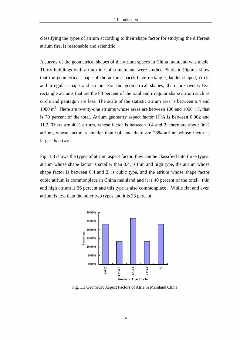
A survey of the geometrical shapes of the atrium spaces in China mainland was made.
Thirty buildings with atrium in China mainland were studied. Statistic Figures show
that the geometrical shape of the atrium spaces have rectangle, ladder-shaped, circle
and irregular shape and so on. For the geometrical shapes, there are twenty-five
rectangle atriums that are the 83 percent of the total and irregular shape atrium such as
circle and pentagon are less. The scale of the statistic atrium area is between 9.4 and
1000 m2. There are twenty-one atriums whose areas are between 100 and 1000 , that
is 70 percent of the total. Atrium geometry aspect factor H2/A is between 0.002 and
11.2. There are 40% atrium, whose factor is between 0.4 and 2; there are about 36%
atrium, whose factor is smaller than 0.4; and there are 23% atrium whose factor is
larger than two.
Fig. 1.3 shows the types of atrium aspect factor, they can be classified into three types:
atrium whose shape factor is smaller than 0.4, is thin and high type, the atrium whose
shape factor is between 0.4 and 2, is cubic type, and the atrium whose shape factor
cubic atrium is commonplace in China mainland and it is 40 percent of the total;thin
and high atrium is 36 percent and this type is also commonplace;While flat and even
atrium is less than the other two types and it is 23 percent.
Fig. 1.3 Geometric Aspect Factors of Atria in Mainland China

1 Introduction
7
1.3 Smoke Control
Knowledge on fire environment with in a building is a vital element of architectural
design. Research results show that smoke is the first and the most rapidly developed
threat to life in fire on a atrium, smoke will bring many problems, and controlling
smoke is essential to providing safety in the atrium spaces[9] [10].
1.3.1 Objectives for Smoke Control
Some form of smoke control (known as smoke management in the USA) is often
required in atrium buildings primarily for life safety purposes. Milke [11] gives five
design objectives for smoke control systems in atrium buildings:
1) Maintain a tenable environment in the means of egress in the atrium during the time
required for evacuation.
2) Confine the smoke in the atrium to a limited region in that space.
3) Limit the migration of smoke into adjacent spaces from the atrium.
4) Provide conditions in the atrium that will assist emergency response personnel in
conducting search-and-rescue operations and locating and controlling the fire.
5) Contribute to the overall protection of life and reduction in property loss.
Milke states that a design may be to achieve either one, or a combination of, these
objectives. Milke also lists a number of ‘hazard parameters’ in which the design
objectives can be evaluated in measurable terms, such as: smoke layer depth; visibility
through the smoke layer; carbon monoxide concentration; temperature rise in the
smoke layer.
1.3.2 Smoke Control Systems
Smoke control systems are defined as engineering systems that includes all the
methods that can be used singly or in combination to reduce smoke production or to
modify smoke movement (ASHRAE and NFPA). The objectives of a smoke control
system are reduce deaths and injures from smoke, reduce properly loss.
Methods to reduce smoke production in atria include the installation of automatic
sprinklers and limitation on the quantity of combustible materials used in the
construction of the building and located on the floor of the atrium Sprinklers are

1 Introduction
8
effective in suppressing fires in floor spaces with limited ceiling heights, but, because
of delayed response, sprinklers may not be effective in suppressing fires in space with
ceiling heights greater than 11 to 15 m or in controlling fires in atria exceeding 20 m in
height. Sprinkler effect is discussed in section 1.9.
Passive methods to modify smoke movement include the use of smoke barriers or draft
curtains to limit smoke incursion into communicating spaces and egress routes.
Another passive method is to allow the smoke to fill the upper portion of the atrium
space while the occupants evacuate the atrium. The latter approach applies only to
large-volume spaces where the smoke-filling time is sufficient for both occupant
response and evacuation.
For those cases in which passive smoke management methods produce insufficient
time for occupant response and evacuation, upper layer mechanical exhaust systems
are frequently used to maintain the smoke level above the occupants until they are able
to evacuate. This system decreases the rate at which the smoke layer descends in the
atrium. A common approach for the design of an upper mechanical exhaust system for
atrium smoke management is to design a system that will maintain the smoke at a
steady clear height assuming a steady-state design fire. Such a system can be designed
using a calculation method based on plume equations in NFPA 92B. This method is
included in the BOCA (1996) and ICBO (1994) building codes. It is the method that
discussed in section 1.4.
There are a number of different smoke control strategies available for atrium buildings.
1) Smoke filling
This approach can be applied to atria which have large volumes, such that smoke
ventilation may not be necessary. This strategy becomes viable when smoke can be
contained in a roof void for the duration of the required safe egress time for the
occupants of the building. In this case, the height of the smoke layer may not reach an
unacceptable value before the fire consumes the available fuel. This approach assumes
that the fire grows at a predictable rate. Fig. 1.4 shows a smoke filling.
Klote and Milke [12] [13] provide empirical relationships to determine the smoke layer
height above the fire with respect to time for both steady and growing fires.

1 Introduction
9
Calculations of smoke layer height are discussed further in section 1.4.
This strategy should only be used if the smoke control designer can demonstrate by
calculation that smoke ventilation is not necessary.
Z
Fig. 1.4 Smoke filling of atrium space
2) Smoke clearance
This approach provides sufficient ventilation to remove smoke from the atrium after
the fire has been suppressed.
3) Smoke and heat exhaust ventilation from the atrium
This strategy uses the buoyancy of the smoky gases from the fire to form a layer above
the occupants of the building, providing a safe means of escape. This form of smoke
control is the main work of this research and is described in detail in the following
section1.3.3.
4) Temperature control ventilation from the atrium
This strategy is used when the height of the smoke layer above the floor is not a critical
design parameter. In this case, smoke exhaust can be used to achieve a maximum value
of the temperature of the layer of smoky gases. This approach allows the use of
materials which would otherwise be damaged by hot gases (e.g. atrium façade
materials which are not fire-resisting).
5) Smoke and heat exhaust from each storey separately
In some cases it may be impractical to provide smoke exhaust ventilation from the
atrium space if the height of rise of the smoke layer from the floor is too large. It may
be beneficial to prevent smoke from entering the atrium altogether (particularly for
fully open atria). This can be achieved by the use of strategically placed smoke curtains
around the atrium space at each storey, and providing smoke exhaust ventilation from
each storey separately.
1 Introduction
10
6) Atrium depressurization
Where the boundary between the atrium space and the adjacent areas is linked by small
openings (e.g. doors gaps, leaky facade), it is possible to prevent smoke from traveling
through these openings by reducing the pressure of the gases in the smoke layer. This
approach is known as depressurization. The purpose of this technique is to prevent
smoke from traveling into the adjacent spaces and does not provide protection to the
atrium space. This technique is similar to that employed for natural environmental
ventilation in atrium buildings.
7) Combination of above strategies (hybrid smoke control)
Various combinations of the above strategies can also be applied, such as atrium
depressurization with smoke and heat exhaust ventilation.
1.3.3 Smoke and Heat Exhaust Ventilation Systems (Smoke Exhaust System)
Smoke and Heat Exhaust Ventilation Systems for atrium buildings provides smoke and
heat exhaust from the upper regions of a building to create a clear layer beneath a
buoyant stratified smoke layer, thus providing conditions for safe means of escape. For
this approach to be effective, it is necessary for the temperature of the gas layer to be
high enough to remain buoyant when at the design height. Smoke Exhaust System may
be naturally driven or mechanically driven (mechanical exhaust fans).
For the smoke exhaust to be effective, it is necessary to provide an adequate amount of
inlet air to replace the hot gases being removed.
Smoke control design in codes and guides is based on the zone fire model concept. In
the zone model, smoke forms an upward-flowing fire plume reaches the ceiling and is
considered to form a perfectly mixed layer under the ceiling of the room of fire origin.
Smoke production depends on the heat release rate of the fire and the height of the fire
plume. Fig. 1.4 depicts the development of the fire plume, the formation of the smoke
layer interface, and the descent of smoke layer as a result of a heat source located in a
position where the fire plume does not meet the wall of the enclose. Klote explains the
physical concepts of the steady fire, unsteady fire, zone fire model, and the fire plume
that are the basis of atrium smoke control. Information about those is not described
further in this report.

1 Introduction
11
In order to properly design smoke exhaust system for a large space, one needs to know
the heat release rate of the expected fire in order to determine the fire size. From that,
one can estimate the amount of smoke. It is then possible to calculate the time needed
for smoke to reach a point that could endanger the occupants and to compare that time
to the egress time. If the smoke layer time is less than the egress time, a smoke
management system should be provided to exhaust smoke at a minimum of the rate at
which the smoke is produced. This is approach used by BOCA (Building Officials and
Code Administrators) National Building Code. It establishes a design criterion that the
smoke management system keeps the smoke layer interface at or above the six-foot
(1,828mm) level for not less than 20 minutes (1200 s). BOCA contains a calculation
method base on NFPA 92B to evaluate compliance with criterion.
1.4 Steady Smoke Layer Interface
In fact, there are two calculation methods to predict the location of the smoke layer
interface in NFPA 92B [14]. One is based on a predictive correlation that generated a
smoke layer interface position at any given time, the other is based on a mass
flow-based calculation correlation to predict the position of a smoke layer interface.
The (BOCA) Building Code codified the NFPA 92B approach. The 1996 BOCA
National Building Code presents two calculation methods for determining the position
of smoke layer interface. They are referred to as “regular” ceiling method to be utilized
for flat-ceiling spaces, and the “irregular” ceiling method, indicating the method to be
utilized for spaces with varying horizontal cross-sectional areas. Two methods are
briefly described as follows:
1.4.1 Regular Ceiling Method
The position of the smoke layer interface, Z, is predicted at any time using the
following equation: 1 3 2 3
1.11 0.28 lntQ H
Z H HA
= −
(1.1)
Where:
Z--height from the floor to the smoke interface, m;
t--time, s;
H--ceiling height above the fire, m;

1 Introduction
12
Q--steady-state heat release rate, kW;
A--cross-sectional area of the atrium, m2.
Equation 1.1 is derived from the steady smoke-filling equation in NFPA 92B. Equation
1.1 is based on plume that has no contact with the walls and for a constant
cross-sectional area with respect to height. This equation is appreciated for A/H2 from
0.9 to 14 and for values of Z greater than or equal to 20% of H.
It is straight using Equation 1.1 to determine a given point (Z) in a defined time period.
The regular ceiling method is presented as a single-point “test” to determine if the
smoke layer interface has reached the critical height (design objective level) in a given
period.
1.4.2 Irregular Ceiling Method
The volume of smoke produced at any height Z is predicted by the following equation
(BOCA):
1 3 3 50.059 0.0015c cVe Q Z Q= + (1.2)
Where
Ve--volumetric rate of smoke production, m3/s;
Qc--convective portion o the heat release rate, kW. (Qc=0.7Q)
For a particular height, Ve defines a volume of smoke produced per unit of time.
Smoke is assumed to be deposited on the ceiling in uniform thickness across the entire
surface. No transit time from the fire to the ceiling, or radically from the center of
plume contact to the perimeter walls, is incorporated into the equation.
Equation 1.2 is derived from NFPA 92B’s mass flow equation:
1 3 3 50.071 0.0018c cm Q Z Q= + (1.3)
Where
m--mass flow rate in plume at height Z, kg/s.
Mass flow is converted to volume flow using the following relationship:
/Ve m ρ= (1.4)
Where
ρ--density of smoke, kg/m3.
1 Introduction
13
By making assumption of the density of smoke to be 1.2 kg/m3 corresponding to 21,
the mass flow equation from NFPA 92B (Equation 3) can be converted to volume flow
equation. Equation 1.2 would represent the “slowest” filling time for an atrium (no
increase in layer temperature above ambient).any increase in layer temperature will
result in faster filling rates than would be predicted by Equation 1.2.
Calculating the layer position by Equation 1.2 is not as straightforward as was the case
for the regular ceiling method. The first iteration uses H as the value for Z. This
method, intended for use in spaces where the horizontal cross-sectional area varies
with height, is to be used in an iterative manner, as opposed to the single-point test
described for the use of the regular ceiling method.
Use of Equation 1.2 is limited to values of Z that are above the limiting elevation. For
information about this, the reader can be referred to Brooks (1997) [15].
1.4.3 Comparison of Methods
Comparison of the two calculation methods for a range of atrium areas and aspect
ratios has been presented by Brooks (1997) [14]. Assuming that:
(1) Atrium A/H2 aspect ratios are between 0.9 and 14;
(2) Fire size are limited to 2110 kW and 4640kW;
(3) The ceiling of the space is flat;
(4) The space has a constant horizontal cross-section area.
Two different building areas were selected and for each cases both calculation methods
were used to predict the position of the smoke layer interface as a function of time for
two different atrium aspect ratios. The results illustrate that the two methods are not
equivalent and will not produce comparable results. There are foreseeable conditions
where the use of the regular ceiling method will require a smoke management system
and the use of the irregular ceiling method will not. The irregular ceiling method is
likely to predict a slower than observed smoke layer interface descent, while the
regular ceiling method is likely to predict a faster than observed descent. Further
analysis was then conducted to reconcile the two methods and develop an approach
that will permit designers to produce comparable hazard analyses regardless of the
method used. A suggested series of adjustments is provided to align the regular ceiling

1 Introduction
14
and irregular ceiling calculation method results over a broad range of interface heights.
For “irregular” calculation method, use of a plume centerline temperature correlation
to adjust the maximum expected layer temperature is suggested as a reconciliation
technique. Equation 1.2 produces the slowest filling since the density correlation
inherent to the coefficient on the right side of the equations is for air at 21 .
Equation1.2 must be adjusted to reflect layer temperatures higher than 21 (ambient
temperature). Brooks recommends that the average temperature of smoke layer is the
temperature of the smoker plume centerline temperature, measured at the critical
height. A density correlation based on 74 smoke layer temperature (approximation
of automatic sprinkler activation temperature) is suggested.
For “regular” calculation method, it is necessary to reevaluate the fundamental
correlation used as the basis for the regular ceiling calculation method, in order to
bring it into agreement with the mass flow used in the irregular ceiling calculation
methods. Brooks argues that six sets of test data are summarized as forming the basis
for the development of the regular calculation method and only two of the test was
conducted in rooms large enough to be considered atria with heat release rates
comparable to expected design fires. Equation 1.1 is predicting smoke layer interface
descent based on a much higher temperature than 74. If Equation 1.1 is to be
continued in use, it will have to be modified to reflect the lower layer temperature in
current atrium design.
1.5 Smoke Exhaust Rate
1.5.1 Equation
Smoke extraction systems are designed to keep the smoke layer high enough to give a
greater clear height. For a steady fire, it is to exhaust smoke from the top of the atrium
in order to achieve a steady clear height. Consider that the only flow into the smoke
layer is from the plume, and the only flow from the smoke layer is the smoke exhaust.
From the principle of conservation of mass for a steady process, the exhaust flow must
equal the flow from the plume. The mass flow equation (NFPA 92B 1995) listed above
can be used to calculate the exhaust flow rate. The adiabatic exhaust temperature is
cp a
p
QT T
mC= + (1.5)

1 Introduction
15
Where
Tp--adiabatic exhaust temperature, ;
Ta--ambient temperature, ;
m--mass flow of exhaust air, kg/s;
Cp--specific heat of plume gases, kJ/(kg· ) .
Using the calculated adiabatic temperature and the ideal gas law, the volumetric flow
rate of smoke can be estimated by Equation 1.4. BOCA uses the following equation to
determine the minimum exhaust rate:
1 3 3 5 0.0015c cVe Q Z Q= + (1.6)
Where
Ve-- volumetric rate of exhaust air, m3/s.
BOCA uses 74 as the temperature of the smoke being exhausted. Alternatively one
can use ambient temperature as an approximation. The exhaust rate is then to be
adjusted in accordance with a table to allow for increase in time for the smoke layer
interface to reach the critical height. The volumetric flow rate defined by Equation 1.6
is used to determine the capacity of the mechanical exhaust system.
1.5.2 Discussion
The basic calculation methods in this section are not application when the design
exceeds the range of applicability of the equations presented.
The calculation method above is only for an ax symmetric plume (a fire located in the
atrium). For a fire located in the communication space, a balcony spill plume or a
window plume is formed. The information about these other plumes, they are
discussed in NFPA 92B (1995) and Chow and Lau.
The design fire has a major impact on the atrium smoke management system. The fire
size is expressed in terms of the rate of heat release. Designs may be based on either
steady or unsteady fires. It is the nature of fires to be unsteady, but the steady fire is a
useful idealization. A steady fire has a constant heat release rate. An unsteady fire is
one that varies with respect to time. Fire protection engineers often use a “t-squared”
approximation for an unsteady fire. A ‘t-squared’ fire is one in which the burning rate

1 Introduction
16
varies proportionally with the square of time , ‘t-squared’ fires are classed (by speed of
growth) as ultra-fast, fast, medium, and slow, based on the time to reach a heat release
rate of 1,055 kW. A ‘t-squared’ fire can be described as follow:
2Q tα= (1.7)
Where
α--growth coefficient. Four types of t-square fire are shown as in Fig. 1.5.
In many applications, use of a steady design fire leads to straightforward and
conservative design. Klote [12] recommends three typical steady design fires of 2,000
kW, 5,000 kW, and 25,000 kW for atria as list in Table 1.1.
Table 1.1 Steady design fire size
Fire scene Heat release
Q/kW
minimum fire of combustible is limited in the atria 2000
minimum fire of combustible is not limited in the atria 5000
maximum fire of combustible is not limited in the atria 25000
For a t-squared fire, the location of the smoke layer interface can be estimated by the
unsteady filling equation from NFPA 92B. The most convenient method of analysis for
the unsteady design approach is by a computer zone fire model, and it is not discussed
further in this research report.

1 Introduction
17
mattressWood palletsFastest burning
Time from ignition(s)
Q(k
w)
100
2110
200
upholstered furniture
4220
6330Ultra-fast
300 400 500
5 ft high
Fast
Slow
700600
Medium
Thin plywood wardrobe
containing plastic foamcontents,fastest if empty orCartons 15 ft high, various
Full mail bages, 3 fthigh pallet satck
interspringCotton/polyester
00
Fig. 1.5 t-square fire
Smoke control system design for atria is more complicated because of the number of
factors that affect air and smoke movement. Atrium smoke management systems have
been mandated by building codes since early 1980s. Early requirements were based on
the air change rate methods, whereby the total volume of the enclosed space was used
to determine airflow rates. Formerly smoke control specifications only use the volume
of atrium space as a criterion for designing smoke extraction system. Obviously it is
not reasonable. Fire size and the risks posed by the position of a smoke layer interface
are not documented in these earlier editions.
The National Fire Protection Association (NFPA) established the Technical Committee
on Smoke Management Systems in 1985. Its first committee project became NFPA
92A, Recommended Practice for Smoke Control Systems, which was published in
1988. The second project was the development of NFPA 92B, Guide for Smoke
Management Systems in Malls, Atria, and Large Areas, first published in 1991.
1.6 Smoke Extraction System Modes and Smoke Exhaust Effectiveness
To protect atrium and all communicating space from smoke, mechanical extraction

1 Introduction
18
system is common installed. There are two possible methods known as ‘smoke
extraction through atrium’ and ‘smoke extraction away from atrium’ [3].
The method of ‘smoke extraction through atrium’ is a conventional method that
provides vents located at the top of the atrium, smoke can be extracted by natural or
mechanical means. The method of ‘smoke extraction away from atrium’ is a method
that provides extraction system located within individual shops and arcade area at each
floor.
Two methods have been compared by Xiong [16]. The results show that advantages of
the method of ‘smoke extraction through atrium’ are its reliable performance, easy
control and convenient commissioning. But its effectiveness is not good, when a fire
locates in the shopping mall adjacent to the atrium and the fire size is very large. For
extracting smoke from the shopping mall adjacent to the atrium, the method of “smoke
extraction away from atrium” is effective. But this is not a effective mean for
extracting smoke provided by a fire in the atrium or migrated into the atrium when a
fire occurs in the compartment connected to an atrium. Yin [17] suggests that the
combination of the two methods is a better method.
There are a number of situations that may detrimentally impact the effectiveness of the
smoke management system. These include obstructions in the smoke plume or the
formation of a pre-stratification layer in the atrium. Under some conditions, another
phenomenon may impact the effectiveness of a smoke control system: air from the
lower (cold) layer can mix with the smoke in the upper layer as it is being exhausted
by the smoke management system. This phenomenon reduces the effectiveness of the
smoke management. As a result, the clear height in the atrium is reduced and people in
some spaces may be exposed to smoke and toxic gases. To study the effects of this
phenomenon on a mechanical exhaust system used for atrium smoke management, a
project was initialed by ASHRAE and the National Research Council of Canada in
1995. The project applied both physical and numerical modeling techniques to atrium
smoke exhaust systems to investigate the effectiveness of such systems [18]. The
experimental facility is a large compartment with dimensions of 9 m by 6 m by 5.5 m.
The design of exhaust system in that study is based on the correlation in NFPA 92B.
The research results demonstrate that, when the exhaust systems operate near or just
below their design capacity, they are effective in extracting gases from the hot layer

1 Introduction
19
without drawing in air from the lower layer. As expected, when the systems operate
well above the required flow rates, fresh air from the lower layer enters the system.
This, however, does not make system ineffective, as the lever of the smoke layer
remains at an acceptable height.
There is concern about exhaust effectiveness for relatively thin smoke layers. There is
possibility of pulling some air from below the smoke layer into the exhaust, and such
reduced effectiveness would result in a smoke layer interface going below the design
value and could expose occupants to smoke. Therefore the project outlined above also
studied the depth of the smoke layer required to prevent atrium exhaust from pulling
air from the lower layer. If the exhaust inlets were located well above the clear height,
the location of the exhaust inlets did not impact the effectiveness of the mechanical
exhaust system. If the exhaust inlets were located at or below the height for which the
mechanical system had sufficient capacity to maintain a clear height, the relatively thin
smoke layer formed below the exhaust inlets. The exhaust gases will include both
entrained air from the lower cold layer and the smoke produced by the fire. Further
research will be needed to determine the parameters that affect the depth of the smoke
layer below the exhaust inlets and scaling of this depth to full scale.
1.7 Smoke Filling Processes and Time Constant
The smoke filling processes in an atrium, simulated by using four zone models, have
been reported by Chow [19]. Zone modes FIRST, CFAST and CCFM.VENTS,
developed at Building and Fire Research Laboratory at NIST, U.S.A., and the NBTC
one-room and two-room hot layer models of the FIRECALC, developed at the CSIRO,
Australia, were used to simulate the smoke filling process. Experimental results on full
scale atrium smoke–filling processes available in the literature were used for
comparing the results on the transient variation of smoke temperature and the
development of the smoke layer predicted by the four zone models. That study
illustrated that a smoke layer would be formed at the ceiling of atrium space and zone
models could be applied to simulate the smoke filling process in an atrium building.
As described above, a survey on the geometrical shapes of atrium spaces in Hong
Kong showed that they can be classified into three main types: cubic, flat, and high.
Simulations of smoke filling processes in those three types of atria using the zone
model FIRST have been reported [20] and the smoke filling times in different types of

1 Introduction
20
atria with the same volume would be very different. It was recommended that a time
constant is to be used for specifying the development of smoke and the smoke filling
time in the atrium space. A time constant, 1τ , describing how fast the atrium will be
filled up with smoke was defined by Chow using the empirical air entertainment rate
equation for an atrium space of volume V, floor area Af, height H, perimeter of fire p
and smoke density ρ:
1
2
0.188
V
p
ρτξ
=
(1.8)
The geometrical aspect factor,ξ , of the atrium space is given by:
2
f
H
Aξ = (1.9)
Note that there are two parts in the expression for the time constant. The first is related
to the properties of a fire and the second part to the geometry of the atrium space.
A correlation of constant time with the time, tr, required to fill 80% of an atrium with
smoke was found. Comparison with experimental data on full-size atria available in the
literature was made and fairly good correlation was obtained:
1rt aτ= (α=1.04±0.2) (1.10)
It is common in design to assume the time of escape to be 2.5 minutes (150 seconds),
and the time required to fill 80% of the atrium with smoke is suggested to be longer
than this value. Therefore, whether a smoke extraction system has to be installed can
be determined by the value of the time constant, rather than by the volume only.
Chow (1997) argued that the time constant, 1τ , was defined through the use of the
empirical equation expressing the mass entrainment rate to the 3/2 power of the clear
height. The equation holds only when the flame tip touches the smoke layer, and the
flame temperature was taken to be 1100 K (827). Another time constant using the
plume equation proposed by Zukoski was defined by Chow:
2 2 32
3
2fA
K H
ρτ
=
(1.11)

1 Introduction
21
Where
2 1
6
5 p rK K Cπ ρ α∞=
And
1 3
1 31 v
p
gK C Q
C Tρ∞ ∞
=
The entrainment coefficient,pα , of the plume lies between 0.0980 and 0.1878, Q is the
heat release rate in kW. Putting in expressions 1K and 1K with the numerical Figures
of ρ∞ (1.2111kg/m3), g(9.81m/s2), pC (1,015J/(kg·K)), T∞ (290K), 0T (1500K), and
vC (1.11) would give:
1 32 2 3
6.245 f
p
A
HQτ
α
=
(1.12)
The second time constant was further evaluated by Chow using three other zone
models—CFAST and CCFM.VENTS developed in U.S. and BRI2 developed in Japan.
Results of the zone modeling simulation supported the fact that the time required to fill
80% of the atrium space with smoke is related to its time constant. A correlation of tr
with the time constant predicted using the zone model FIRST is given by:
20.798rt τ= (1.13)
The correlation relation is supported by the simulation results of three other zone
models–CFAST, CCFM.VENTS, and BRI2. Experimental data on the smoke filling
process available in the literature were used to evaluate this time constant. The value of
time constant was recommended to specify the smoke filling time for an atrium space
for design purposes. Whether a smoke extraction system has to be installed can be
determined by checking whether the atrium with a certain time constant will give a
time required to fill 80% of the atrium with smoke that is less than 2.5 minutes (150s)
using Equation (1.13).
1 Introduction
22
1.8 Airflow for Smoke Control between Atrium and Communicating Spaces
Airflow can be used to prevent smoke flowing from a fire in a communicating space to
atrium and also can be used to prevent smoke flowing from the atrium to the
communicating space. If it is desired to use airflow to prevent smoke producing in the
communicating space from flowing into the atrium, the air needs to be exhausted from
the communicating space. The exhaust flow rate needs to be sufficient to result in an
average air velocity in the opening between the communicating space and the atrium to
prevent smoke flow. NFPA 92B (1995) recommends the following equation for the
limiting velocity to prevent smoke backflow:
( )00.64
f
f
gH T TV
T
−= (1.14)
Where
V--average air velocity, m/s;
g--acceleration of gravity, m/s2;
H--height of opening, m;
Tf--temperature of heated smoke, K;
T0--temperature of ambient air, K.
Air can be supplied to a communicating space to achieve a specific average velocity at
the opening to the atrium. This velocity should be such that smoke flow to the
communicating space is prevented. For opening locations below the smoke layer and 3
m above the base of the fire, the equation (NFPA 92B) for this velocity is
1 3
0.057Q
VZ
=
(1.15)
Where
V--average air velocity, m/s;
Q--heat release rate of the fire, kW;
Z--distance above the base of the fire to the bottom of the opening, m.
If the velocity calculated from the above equation is greater than 1 m/s, then a velocity
of 1 m/s should be use. This limitation was made out of concern that greater velocities
could disrupt the plume flow and have an adverse effect on atrium smoke management.
For openings above the smoke layer interface, Equation 15 should be used to calculate

1 Introduction
23
the velocity.
Klote (1997) addressed that research should be needed concerning use of airflow for
smoke control between the atrium and communicating spaces. There is insufficient
information to evaluate whether these systems provide any significant level of
protection to life or if their sole benefit is property protection. The issue of evaluation
of the potential benefit of these systems is further complicated by the concern about
airflow supplying combustion air for a fire and information is needed to evaluate the
potential benefits of these airflow systems. If the benefits support use of these systems,
research is needed to develop new approaches for sprinkled fires.
1.9 Sprinkler Effect
Automatic sprinkler systems are installed in many buildings including atria to control
fire. Chow [3] indicates that there are three key points to be considered in assessing the
performance of an atrium sprinkler: the possibility of actuating the sprinkler in a
pre-flashover fire; the thermal response of the sprinkler head and the interaction
between the water spray and smoke layer.
Theoretical analysis is as follow. The gas temperature rise at the ceiling can be roughly
estimated by the expression:
2 3
5 3
0.22g
QT
H∆ = (1.16)
Where
gT∆ --gas temperature rise at ceiling, K;
Q--rate of heat release from the fire plume, kW;
H--height of atrium, m.
Normally, the sprinkler heads would have a temperature rating between 57 and 68
. If the ambient air temperature is 20 and the heat release rate is 5 MW, then the
sprinklers will only be actuated if the atrium height is less than 20m. A normal
sprinkler head installed by a fire is of less than 5 MW. For an atrium of 30m height, the
value of Q actuating a sprinkler head would be 17MW or more.
1 Introduction
24
The time required for actuating a sprinkler head up to an excess temperature of 50
is:
188ln50
ga
g
Tt
T
∆= ∆ − (1.17)
Where
ta--actuation time, s;
τ--time constant, m3/2s3/2. (for the normal sprinkler head, τ=188)
For an atrium of height 15m with a 5 MW fire, the time required for actuation (normal
head) is about 6 minutes. Therefore, normal sprinkler head is not suitable for the
purpose. A fast response sprinkler head seems to be more appropriate as the time
constant, τ, in the Equation 1.18 will drop to a value about 50 m3/2s3/2, the actuation
time becomes much shorter. Similar ceiling height of 15 m requires only 1 minute for
actuation.
Even when the sprinkler head is actuated, the smoke is cooled by the discharged water
spray and loses its buoyancy. This together with the reaction force due to the air drag
experienced by the water droplets would pull the smoke layer downward and give
adverse effects on the occupants still staying inside the atrium space. If a smoke
extraction system is installed, the effectiveness of it might be reduced due to this strong
downward force acting on the smoke layer. Therefore the provision of a mechanical
smoke extraction system seems essential. It is doubtful whether sprinkler should be
installed in a high headroom atrium.
Chow and Chau (1994) also indicate that automatic sprinklers installed at the atrium
ceiling might not be good in controlling an atrium fire. Mawhinney (1994) suggests
that a review of current, strategies and assumptions about the behavior of cold smoke
in atria in sprinkled building should be conducted. The scenario of smoke from a
shielded, sprinkled fire in a floor area adjacent to an atrium could be considered.
ASHRAE has a research project to study the hazard to life resulting from sprinkled
fires in a communication space.
1.10 Research Objective
Currently, there are a number of calculation methods available to designers for smoke

1 Introduction
25
control of atrium buildings. And there are also many researches on smoke movement in
atrium building. Different geometrical arrangements of fire inside a building could lead
to different entrainment, and hence different plume expressions.
The amount of air entrained into the plume will depend on the configuration of the
plume produced. Milke identified five configurations of smoke plume which may exist
within atrium buildings, these are:
1) Axisymmetric plume
An axisymmetric plume is generally expected from a fire located near the centre of an
atrium floor. This type of plume is typically remote from any walls and air is entrained
around all sides of the plume. Entrainment of air will occur over the full height of the
plume until it reaches the interface with a smoke layer which may have formed above.
A classical analysis of axisymmetric plumes has been carried out by Morton, Taylor
and Turner [21].
2) Wall plume
A plume which is generated from a fire against a wall is known as a wall plume.
Zukoski[22] developed a wall plume entrainment correlation based on “mirror
symmetry”. Work by Poreh and Garrad has highlighted that further research on wall
plume entrainment is desirable.
3) Corner plume
A plume which is generated from a fire located in the corner of a room, where the
walls form a 90o angle, is known as a corner plume. Zukoski [23] treated the corner
plumes in a similar manner to a wall plume with the use of “mirror symmetry” for
plume entrainment. Again, work by Poreh and Garrad has demonstrated that further
research is desirable for corner plume entrainment.
4) Spill plume
A spill plume is a vertically rising plume resulting from an initially horizontally
moving smoke layer which then subsequently rises at a spill edge (e.g. at an opening
onto an atrium space). This type of plume is the major focus of this work as is
described in detail in the following section 6.

1 Introduction
26
5) Window plume (door plume)
A window plume is a plume which flows from a window (or doorway) into an atrium
space. Typically, window plumes are generated from post-flashover fires. An
entrainment correlation was developed by Heskestad, by comparing the air entrainment
for a window plume with that of an axisymmetric plume. The window plume
entrainment correlation is given by Klote and Milke [24].
Full-scale burning tests were performed to derive the plume expressions empirically.
However, widespread use of this approach is not economically feasible and
experimental data are limited. With the rapid development of computational fluid
dynamics (CFD), it is now possible to assess the plume equations, and CFD might be
regarded as a useful tool in solving some plume flows in buildings. There had been
earlier works on assessing the temperature and mass flux formulae for some expressions
on axisymmetric plumes and balcony spill plumes with CFD packages.
However, there is less research on the effect of fire location on plume entrainment,
balcony plume entrainment and smoke movement in large space with the sloping floor.
There are three specific objectives which this report aims to address, these objectives
are described below:
1) Plume entrainment in a large space with different fire location
2) Balcony plume in a large space building with communicating compartment
3) Smoke movement in a large space with sloping floor
Computational Fluid Dynamics and scale model experiments are two possible methods
for the determination of smoke movement in the large building.

2 Governing Equations and Large Eddy Simulation
27
2 Governing Equations and Large Eddy Simulation
Smoke and fire movement in a building is usually a turbulent flow with significant
density variation due to large temperature gradients. In the field of fire protection
engineering, zone models are frequently used for study of fire hazards or design of
protections systems. In recent years, however, computational fluid dynamics (CFD)
has shown great value as a tool to study smoke and fire movement. In the CFD
approach a limited number of assumptions are made and a high-speed digital computer
are used to solve the resulting governing fluid dynamic and heat transfer equations.
CFD is divided into three types:
(1) Direct numerical simulation (DNS);
(2) Reynolds averaged Navier-Stokes equation (RANS);
(3) Large eddy simulation (LES).
DNS requires the grid resolution to be as fine as a viscously determined scale. Using
DNS with simple geometry and a low Reynolds (Re) number flow provides very
valuable information for verifying or improving turbulence models. However, the
number of DNS grid points required for the resolution of all scales increases
approximately as Re. This creates difficulty in handling high Re numbers with strong
buoyant flows, such as fire and smoke movement problems in realistic conditions.
Large-eddy-simulation (LES) for solving the fluid dynamic equations of 3D elliptic,
reacting flow.
LES is considered somewhere between DNS and k-e turbulence model computations.
The basic idea behind the LES technique is that eddies that account for most of the
mixing is large enough to be calculated with reasonable accuracy from the equations of
fluid dynamics. The small-scale eddy motion can be crudely accounted for. The LES
approach systematically captures more and more of the dynamic range contained in the
Navier-Stokes equations as the spatial and temporal resolution is improved. This
approach to the field modeling of fire phenomena emphasizes high enough spatial and
temporal resolution with an efficient flow solving technique.
In a LES calculation where the grid is not fine enough to resolve the diffusion of fuel
and oxygen, an adjusted mixture fraction-based combustion model is used. The

2 Governing Equations and Large Eddy Simulation
28
large-scale transport of combustion products can be simulated directly, but combustion
processes occurring at small length and time scales are represented in an approximate
manner.
2.1 Governing Equation
Smoke movement is a compressible physics phenomenon and it should be satisfied by
the following compressible flow equations:
( ) 0ii
ut x
ρ ρ∂ ∂+ =∂ ∂
(2.1)
( ) ( ) 2
3ji i
i i j ij i j j i i j
uu upu u u g
t x x x x x x xρ ρ µ µ ρ
∂∂ ∂∂ ∂ ∂ ∂ ∂+ = + + − + ∂ ∂ ∂ ∂ ∂ ∂ ∂ ∂ (2.2)
( ) ( )p j pj j j
Tc T u c T q
t x x xρ ρ λ
∂ ∂ ∂ ∂+ = + ∂ ∂ ∂ ∂ (2.3)
pRT
ρ= (2.4)
Here, all symbols have their usual fluid dynamical meaning: is the density, u the
velocity vector, p the pressure, g the gravity vector, cp the constant pressure specific
heat, T is the temperature, λ is the thermal conductivity, t is the time, q is the
prescribed volumetric heat release, R is the gas constant equal to the difference of the
specific heats R=Cp-Cv.
2.2 Turbulence Model
LES solves the large eddy motion by a set of filtered equations governing the
three-dimensional, time-dependent movements. The small eddies are modeled
independently from the flow geometry.
The filtering operation decomposes a full field,( ),x tφ , into a resolved component
( ),x tφ and a sub-grid scale component ( ),x tφ ′ [25]. The resolvable-scale component,
( ),x tφ , is obtained from its full field, ( ),x tφ , by employing a filter ( ),G x ∆ of
specified width ∆ :

2 Governing Equations and Large Eddy Simulation
29
( ) ( ), ( , ) ,x t G x x x t dxφ φΩ
′ ′ ′= − ∆∫ (2.5)
Where, Ω is the interested domain. The unresolved field, component, ( ),x tφ is
given by:
( ) ( ) ( ), , ,x t x t x tφ φ φ′ = − (2.6)
With the finite volume method used in the LES formulation, it seems natural to define
the filter width as an average over a grid volume ( ( )1 3
i x y z∆ = ∆ ∆ ∆ ).
In most LES involving compressible flows, the variables are Favre-filtered (i.e. density
weighted) by /f fρ ρ=% (f is a variable, and ρ is the density) in order to consider
density fluctuations.
Applying the filtering operation to each term in the conservation equations of mass,
momentum, energy and species, and decomposing the dependent variables (u; v; w; p;
etc.) into resolved and subgrid components results in the filtered governing equations,
shown below:
0l l i
i
u
t x
ρ ρ∂ ∂+ =∂ ∂
(2.7)
( )*
l j ijl j i ij
i i
uu u p
t x x
ρ τρ σ
∂ ∂∂+ − − = −∂ ∂ ∂
(2.8)
( ) ( )i i ij ij HR V d v
i i i i
h u h q Qp pu Q C
t x x t x x
ρ ρσ
∂ ∂ ∂ ∂∂ ∂+ + − − − = − − Π + Σ∂ ∂ ∂ ∂ ∂ ∂
(2.9)
Where iu is the filtered velocity, ρ is the filtered density, p is the filtered
pressure, h is the filtered enthalpy per mass, CV the constant volume specific heat,
and HR
Q the filtered volumetric heat release rate that is represented the following
section. Here, the diffusive fluxes are given by:
22
3ij ij ij kkS Sσ µ µδ= − (2.10)

2 Governing Equations and Large Eddy Simulation
30
ii
Tq k
x
∂= −∂
(2.11)
Where µ is the molecular viscosity, and k is the thermal conductivity corresponding
to the filtered temperature T. The effect of the SGS terms appears through the SGS
stresses Sij, the SGS heat flux Qi, the SGS pressure dilatation dΠ , and the SGS
contribution to the viscous dissipation dΠ . These quantities are defined as,
( )ij i j i ju u u uτ ρ= − (2.12a)
( )i i iQ u T u Tρ= − , d kk kkpS pSΠ = −
v ij ij ij ijS Sσ σΣ = − (2.12b)
2.3 Sub Grid Scale Models
The sub grid scale (SGS) models for the unresolved terms in the momentum and
energy equations must be carefully treated. Among the various SGS turbulence models,
such as the mixed model and the two parameter mixed model for compressible
turbulence offered the best trade off between accuracy and cost. In the thesis, the
modeling of the SGS stresses has received comparatively more attention than the other
unclosed terms (2.2b) for compressible flows. The anisotropic part of the SGS stresses
is treated using the Smagorinsk model, while the Skkis modeled with a formulation
developed by Yoshizawa],
223 3ij ij
ij kk R ij kk R ijC S S S C aδ δ
τ τ − = − ∆ − =
(2.13a)
2 22kk l lC S S Cτ ρ β= ∆ = (2.13b)
223ij
ij ij kka S S Sδ
ρ = − ∆ −
,
222 Sβ ρ= ∆ (2.13c)
Where CR and CI are model constants
Yoshizawa proposed an eddy -viscosity model for weakly compressible turbulent flows
using a multi-scale, direct-interaction approximation method and suggested that
CR=0.0256 and CI=0 based on theoretical arguments.

2 Governing Equations and Large Eddy Simulation
31
The SGS heat flux (2.12b) needs to be closed. A simple approach is to use an eddy
diffusivity model of form
2
Pr PrT
i RT j T j
ST TQ C
x x
ρρν ∆∂ ∂= − = −∂ ∂
(2.14)
The turbulent Prandtl number PrT can be fixed (e.g PrT=0.7, PrT=0.4)
2.4 FDS Introduction
The CFD model used in this study was Fire Dynamics Simulator (FDS) which has
been developed by McGrattan et al of the National Institute of Standards and
Technology.
This model numerically solves a form of the Navier-Stokes equations appropriate for
low-speed, thermally driven flows typically generated by smoke and heat transport
from fires. The fundamental equations and the numerical algorithm within the model
are given by McGrattan et al and are discussed in section 2.2 and 2.3. In this study,
FDS was set to treat turbulence by means of the Smagorinsky form of Large Eddy
Simulation (LES).
A complete description of the FDS model is given in references [26].Inputs required by
FDS include the geometry of the structure, the computational cell size, the location of
the ignition source, the energy release rate of the ignition source, thermal properties of
walls, ceilings, floors, furnishings, and the size, location, and timing of door and
window openings to the outside which critically influence fire growth and spread.
The results of the model have been visualized using the post processing tool called
Smokeview (version 3.1) developed by Forney and McGrattan. Smokeview is a
3-dimensional imaging software tool which can show isosurfaces (e.g. temperature,
mixture fraction) and 3D data files (e.g. temperature, velocity and pressure).
Smokeview is a scientific visualization program that was developed to display the
results of an FDS model computation Smokeview allows the viewing of FDS results in
three dimensional snapshots or animations. Smokeview can display contours of
temperature, velocity and gas concentration in planar slices. It can also display
properties with isosurfaces that are three-dimensional profiles of a constant value of

2 Governing Equations and Large Eddy Simulation
32
the property. Iso-surfaces are most commonly used to provide a three-dimensional
approximation of the flame surface where fuel and oxygen are present such that flames
may exist.
From the predicted airflow pattern and temperature fields, the smoke layer interface or
thermal stratified layer, height is obtained by inspecting the positions where there are
sharp changes of temperature in the vertical direction. The hot layer temperature is
taken to be the average value over all at the control cells in the smoke layer.
3 Similar Theory and Dimensionless Numbers
33
3 Similar Theory and Dimensionless Numbers
Scale model experiments are based on the similarity principle. Similarity criterion
numbers can be found from the governing equations of smoke flow.
3.1 Similar Theory
The governing equations for mass flow, energy flow and contaminant flow in a room
will be the continuity equation, Navier-Stokes equations, the energy equation and the
mass transport equation, respectively.
The continuity equation for an incompressible flow is given by the following
expression:
0u v w
x y z
∂ ∂ ∂+ + =∂ ∂ ∂
(3.1)
u, v, and w are the instantaneous velocities in the three coordinate directions x, y, z. It
means velocity is the sum of a mean value and a turbulent fluctuation, such as u is the
sum of a mean value u and turbulent fluctuation u′ (u u u′= + ).
The Navier-Stokes equation in the direction of gravity(y-direction) is given by the
expression:
( )2
02 2 2( )
v v v v p v v vu v w g T T
t x y z y x y zρ µ ρ β ∂ ∂ ∂ ∂ ∂ ∂ ∂ ∂+ + + = − + + + − − ∂ ∂ ∂ ∂ ∂ ∂ ∂ ∂
(3.2)
p, T, t are temperature and time, respectively, and T0 is a reference temperature (supply
temperature). Andρ , β , µ and g is density, volume expansion coefficient, viscosity
and gravitational acceleration, respectively. The density and the viscosity are in
principle functions of the instantaneous temperature T, but except for the gravitational
term the effect is ignored due to the level of temperature differences that occur in
practice. The term ( )0T T− expresses the influence of the temperature in the
gravitational term in a formulation called Boussinesq approximation.
The energy equation is given by the expression:

3 Similar Theory and Dimensionless Numbers
34
2 2 2
2 2 2( )p
T T T T T T Tc u v w q
t x y z x y zρ λ ∂ ∂ ∂ ∂ ∂ ∂ ∂+ + + = + + + ∂ ∂ ∂ ∂ ∂ ∂ ∂
(3.3)
cp, λ, and q are specific heat, thermal conductivity and heat release rate of heat source.
Where, in the fire location there is a heat source and its power is q, otherwise in the
other areas q is equal to zero.
The equations (3.1) to (3.3) describe the velocity u, v, w, the temperature distribution T
and pressure distribution p. The variables can also be used for calculation for air
volume flow, convective air movement.
It should be noted that radiant heat transfer, which can be an important part of the heat
flow in a building, has not been considered.
According to the similarity principles, the governing equations in a no dimensional
form can be developed. The defining dimensionless, independent variables as:
*0/x x h=
*0/y y h=
*0/z z h= (3.4)
Where, h0 is a characteristic length of interest in the problem. A typical characteristic
length in ventilation problems is the height of supply slot h0 or the square root of the
supply area. The height of a hot or a cold surface can also be used as characteristic
length in situations where free convection is the most important problem as for
example in the case of cold downdraught in an atrium at low outdoor temperatures. In
fire smoke movement, a typical characteristic length h0 is the height of the model.
The velocities:
*0/u u u= *
0/v v u= *
0/w w u= (3.5)
Where u0 is a characteristic velocity, normalized by the supply velocity u0 found from:
0 0 0/u Ve A= (3.6)
Where Ve0 is the volume flow rate to the inlet and A0 is the supply opening area of
inlet.
* 0
0R
T TT
T T
−=−
(3.7)
Where, T0, TR is supplement temperature, exhaust temperature respectively.

3 Similar Theory and Dimensionless Numbers
35
Pressure p, heat source Q and the independent variable time t are normalized by the
following expressions:
* 20/p p uρ= (3.8)
*
0
Q= (3.9)
*0 /t tu h= (3.10)
Where, Q0 is a characteristic heat release of the fire source.
Equations (3.5), (3.6), (3.7), (3.8), (3.9) and (3.10) are substituted into equations (3.1)
to (3.4) and the following dimensionless governing equations are obtained
* * *
* * *0
u v w
x y z
∂ ∂ ∂+ + =∂ ∂ ∂
(3.11)
( )* * * * * 2 * * *
* * * *0
0* * * * * *2 *2 *2 2
0 0 0
R
ghv v v v p v v vu v w T T T
t x y z y h u x y z u
βµρ
∂ ∂ ∂ ∂ ∂ ∂ ∂ ∂+ + + = − + + + − −
∂ ∂ ∂ ∂ ∂ ∂ ∂ ∂
(3.12)
* * * * 2 * 2 * 2 *
* * * *0
* * * * *2 *2 *2 2
0 0 0 0 0 0 0
)p p
QT T T T T T Tu v w Q
t x y z c h u x y z c u T h
λρ ρ
∂ ∂ ∂ ∂ ∂ ∂ ∂+ + + = + + +
∂ ∂ ∂ ∂ ∂ ∂ ∂
(3.13)
It is obvious that the following dimensionless numbers appear in the equations:
( )0 020
Rgh T TAr
u
β −= (3.14)
0 0eh u
Rρ
µ= (3.15)
Pr pcµλ
= (3.16)
0 02 1/ 2 5/ 2
0 0 0 0 0 0II
p p
Q QD
c u T h c g T Lρ ρ= = (3.17)
Ar, Re and Pr DII are called Archimedes number, Reynolds number, Prandtl number
and Damlohler's ratio respectively.
The Archimedes number may be considered as a ratio of thermal buoyancy force to
inertial force, while the Reynolds number may be looked upon as a ratio of inertial

3 Similar Theory and Dimensionless Numbers
36
force to viscous force. The Reynolds number can also be considered as a ratio of
turbulent diffusion to laminar diffusion. The Prandtl number is the ratio of momentum
diffusivity to thermal diffusivity. Damlohler's ratio is the ratio of heat release rate by
burning to convection.
3.2 Similarity Principles and Conditions for Model Experiments
The general conditions for scale model experiments with flow in a room are:
1) Identical dimensionless sets of boundary conditions, including geometry, in room
and in model.
2) Identical dimensionless numbers, equations (3.10) to (3.12), in the governing
equations for the flow in the room and in the model.
3) The constantsρ , β , µ in the governing equations (equation (3.1) to (3.5)) should
only have a small variation with in the applied temperature and velocity levels.
The requirements of identical dimensionless boundary conditions are met when the
model is geometrically similar to full scale in the details that are important for the
volume flow and the energy flow.
In smoke movement experiments the problem can be deal with the Reynolds number is
high and the flow pattern is governed mainly by a fully developed turbulence. The
Archimedes number or Froude number is the only important dimensionless number
and they can both be fulfilled by an appropriate combination of velocity and
temperature difference.
In the fire small scale model experiment design, Reynolds number is large enough that
the movement is turbulent flow with fully developed flow. The experiments are
characterized by the Archimedes number and Damlohler's ratio:
( )0 020
Rgh T TAr idem
u
β −= = (3.18)
02
0 0 0 0II
p
QD idem
c u T hρ= = (3.19)
The reduced scale model is geometric similarity to the full scale model. The geometric

3 Similar Theory and Dimensionless Numbers
37
scaleλ is as follow
.mL
f
Lconst
Lλ= = (3.20)
( )/m F m fx x L L= (3.21)
Where
L--length;
x--location;
Subscripts;
F--full-scale;
m--reduced-scale model.
The temperature is the same in the corresponding location between the reduced scale
model and full scale model.
m fT T= (3.22)
According to the equation (3.16), velocity and volumetric rate scaling relationship is as
follow: 1 2
1 2mm f f L
f
Lv v v
Lλ
= =
(3.23)
5 2
5 2mm f f L
f
LVe Ve Ve
Lλ
= =
(3.24)
Where
v--velocity, m/s;
Ve--volumetric inlet air supply rate or smoke exhaust rate, m3/s.
According to the equation (3.17) and (3.20), the fire heat release rate scaling
relationship is as follow:
( )5 2
, , /c m c F m FQ Q L L= (3.25)
Where
Qc--convective heat release rate, KW.

3 Similar Theory and Dimensionless Numbers
38
Scaling relationships for the physical modeling are shown as in Table 3.1.
Table 3.1 Scaling relationships for the physical modeling
location ( )/m f m fx x L L=
temperature m fT T=
velocity ( )1 2/m f m fv v L L=
heat release rate ( )5 2
, , /c m c f m fQ Q L L=
volumetric rate ( )5 2 5 2/m f f m f LVe Ve L L Ve λ= =
Where
x--position;
L--length, m;
T--temperature, K;
v--velocity, m/s;
Ve--volumetric exhaust rate, KW;
Qc--convective heat release rate, KW.
Subscripts
F--full-scale;
m--reduced-scale model.
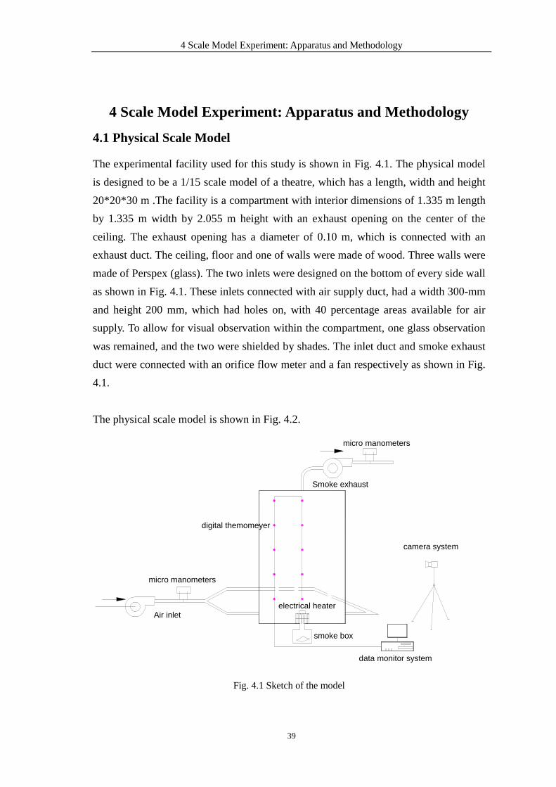
4 Scale Model Experiment: Apparatus and Methodology
39
4 Scale Model Experiment: Apparatus and Methodology
4.1 Physical Scale Model
The experimental facility used for this study is shown in Fig. 4.1. The physical model
is designed to be a 1/15 scale model of a theatre, which has a length, width and height
20*20*30 m .The facility is a compartment with interior dimensions of 1.335 m length
by 1.335 m width by 2.055 m height with an exhaust opening on the center of the
ceiling. The exhaust opening has a diameter of 0.10 m, which is connected with an
exhaust duct. The ceiling, floor and one of walls were made of wood. Three walls were
made of Perspex (glass). The two inlets were designed on the bottom of every side wall
as shown in Fig. 4.1. These inlets connected with air supply duct, had a width 300-mm
and height 200 mm, which had holes on, with 40 percentage areas available for air
supply. To allow for visual observation within the compartment, one glass observation
was remained, and the two were shielded by shades. The inlet duct and smoke exhaust
duct were connected with an orifice flow meter and a fan respectively as shown in Fig.
4.1.
The physical scale model is shown in Fig. 4.2.
smoke box
electrical heater
Smoke exhaust
micro manometers
Air inlet
digital themomeyer
data monitor system
camera system
micro manometers
Fig. 4.1 Sketch of the model

4 Scale Model Experiment: Apparatus and Methodology
40
Fig. 4.2 The physical scale model
4.2 Instrumentation
In the test compartment there were thermocouple trees to test the smoke temperature.
The electrical heater was used as the fire source. The smoke was produced by smoke
box using fuming liquid.
Frequency conversion method was used to change the fans rotation speed. The two
transducers were used for the air supplement fan and smoke exhaust fan respectively.
And then the designed inlet air volume rate and exhaust rate could be obtained by
changing the electric frequency.
The volume flow rate was measured using the throttle aperture mounted in the each air
supply duct and smoke exhaust duct. Firstly the throttle aperture ducts were
standardized. The rate of the smoke exhaustion and inlet air were deduced from the
static pressure difference measured by the micro manometers and the temperature
measured by the thermocouple. There is a ruler put in the model to measure the smoke

4 Scale Model Experiment: Apparatus and Methodology
41
layer height.
The two sets of throttle duct were used in the experiment. One is large and the other is
small. Their equations for calculating the volumetric rate are as follow:
For the small duct set, the relationship between the pressure difference and volumetric
rate are as follow:
2.049770.00998p Ve∆ = ⋅ (4.1)
0.48799.465Ve p= ⋅ ∆ (4.2)
Where,
p∆ --mmH2O;
Ve --m3/h.
For the large duct set, the pressure difference and volumetric rate are as follow:
2.039750.005957 vp q∆ = ⋅ (4.3)
0.49025612.325Ve p= ⋅ ∆ (4.4)
1.2mVe Ve
ρ= ⋅ (4.5)
p∆ --Pa
vq --m3/h;
Ve --m3/h;
mVe --the practical volumetric rate in the test.
The volume rate can be calculated by the pressure difference tested in the experiment.
Inlet air velocity may be calculated by the volumetric rate and actual inlet areas.
ein
VV
A= (4.6)

4 Scale Model Experiment: Apparatus and Methodology
42
4.3 Test Methods
Before the test, the exhaust and inlet fans were opened. The transducers were adjusted
to ensure the designed air supply rate and smoke exhaust rate according to the
experimental cases. The smoke producer and electrical heater were turned on for
several minutes. When the air flow in the model began to the steady, then carefully
made the smoke filled the smoke box, and the air pump was switched on at a fixed
voltage to obtain a uniform outlet velocity.
In the experiment beginning the smoke entered into the compartment, the smoke plume
rose quickly up to the ceiling, then the plume spread horizontally and down, eventually
formed steady smoke depth and then stopped at a certain height in several minutes. The
smoke layer height, smoke temperature and inlet air temperature were measured during
the test.
The smoke layer height was deduced from the temperature profile collected by
thermocouple and the smoke image observed or caught by video. Temperature data
were recorded every ten seconds during the test times on a multi-channel data
acquisition system. The conditions in the test space were observed by a video camera.

5 Experiment and FDS Simulation on Plume Entrainment for the Different Fire Location
43
5 Experiment and FDS Simulation on Plume Entrainment for
the Different Fire Location
The volume of smoky gases generated from a fire within an atrium is highly governed
by the mount of air entrained into the rising smoke plume. The volume of smoke must
be calculated in order to determine the required fan capacity or vent area for a smoke
ventilation system. The amount of air entrained into the plume will depend on the
configuration of the plume produced. Milke identified five configurations of smoke
plume which may exist within atrium buildings.
The axisymmetric plumes were discussed in this section. The series of experiments and
FDS simulations with the steady-state fire were conducted to study the effect of the fire
location on smoke movement or entrainment rates of air from the surroundings.
The fire source was placed in the four different locations on the floor, shown as in Fig.
5.1 and Table 5.1. The inlet air supply rate and smoke exhaust conditions in each fire
location experiments were shown in Table 5.1.
Table 5.1 Different fire location and designed fire power in experiment
85
376
C
85
Heat source
37685
668
668
668
A
B
D
Fig. 5.1 Location of heat source on the floor
Scheme A(center) B(beside the wall) C(corner) D(Between a and C)
Heat release rate(W) 300/500 300 300/500 300
X position(m) 668 668 85 376
Y position(m) 668 85 85 376
All dimension in mm

5 Experiment and FDS Simulation on Plume Entrainment for the Different Fire Location
44
Three trees of the thermocouple were collocated in the diagonal of the model shown as
Fig. 5.2. A set of 6 thermocouples with 380mm intervals was vertically placed at the
center of the compartment over the fire source. A second set of 6 thermocouples with
38-mm intervals was also vertically placed at the corner of the compartment, and a
third set of 3 thermocouples with 380mm, 155mm intervals was also vertically placed
at the other corner of the compartment, as shown in Fig. 5.2.
202 7
F1
1335125
18 668
21
x x
1335
33422
22
21 16
y
334tree3
tree1334
tree2668
z 18 17
1335 10
334
1
380
380
4 1911
5 12
6 13
2055
380
380
tree2
3
tree1 155
380
148
9 15
155
23tree3
Fig. 5.2 The arrangement of thermocouples
5.1 Experimental Conditions
The series of experiments with the steady-state fire on filling (no ventilation) and
ventilation condition were conducted. The smoke exhaust rate and inlet air supply rate
were designed in order to get a steady smoke layer height.
The inlet air supply rate and smoke exhaust conditions were summarized in Table 5.2.
5.2 Smoke Filling
Smoke filling experiments has been conducted that the steady-state fire located in the
four different location on the floor with heat release 300W and 500W.
All dimension in mm

5 Experiment and FDS Simulation on Plume Entrainment for the Different Fire Location
45
Table 5.2 Inlet air supply rate and smoke exhaust rate in the experiment
case Inlet air supply rate
(m3/s)
Inlet air velocity
(m/s)
Smoke exhaust rate
(m3/h)
Smoke exhaust velocity
(m/s)
1 0.006 0.031 22.9 0.811
2 0.009 0.044 32.6 1.154
3 0.012 0.060 44.2 1.564
4 0.016 0.079 57.8 2.046
5 0.020 0.097 71.2 2.517
6 0.025 0.122 89.8 3.178
7 0.030 0.147 108.2 3.828
8 0.044 0.215 157.9 5.585
9 0.058 0.283 207.6 7.342
10 0.071 0.350 257.3 9.099
11 0.085 0.418 307.0 10.856
12 0.099 0.486 356.6 12.614
To obtain more information about the smoke movements in large space building, CFD
simulations were finished by adopting large eddy simulation (LES) technique. In the
simulations, the smoke movement was simulated by a steady fire, and the combustion
stoichiometry is similar to polyurethane. The initial temperature was set according to
the temperature measurements in the experiments.
Fig. 5.3 shows the measured results of vertical temperature distribution of the
thermocouple tree 1 located in the southwest corner as a function of the time for the
300W fire located in the center (Fire 1).

5 Experiment and FDS Simulation on Plume Entrainment for the Different Fire Location
46
Measured
0
5
10
15
20
25
30
0 0.5 1 1.5 2
height(m)
T(
)
30s 60s 120s 150s 180s 210s 0s
Fig. 5.3 Test vertical temperature distribution (tree 1) versus time in smoke filling (Center fire)
It is obvious that at the beginning of the ignition, the temperatures are almost constant
from the bottom to the top of the thermocouple tree. It should be noted that the
experimental data taken from the measurements during 1-3.5 minutes show that the
temperatures close to the ceiling increase markedly and then all the temperatures
increase uniformly. The descent of the smoke layer is very quick at the first period but
slows down later. This is attributed to the fact that the rate of air entrainment from the
lower layer decreases as the smoke layer descends further. The vertical temperature
distribution with smoke tends to be non-uniform with a temperature gradient from the
floor to the ceiling. Temperature continuously increased with height up to the region
near the ceiling. Stratification effect can be discerned from the temperature changes
along the vertical direction at given times. The temperature distribution indicates a
distinct interface between the hot upper layer and the relatively cool lower layer, being
thick transition zone. The hot gas temperature is not too high. It also indicates that it
takes about a litter less than 3 minutes for smoke to descend the floor in the model.
The photographs of smoke filling prediction captured by a digital camera for the fire
located in the center and corner are shown in Fig. 1 in Appendix A.

5 Experiment and FDS Simulation on Plume Entrainment for the Different Fire Location
47
Simulated
0.0
5.0
10.0
15.0
20.0
25.0
30.0
0 0.5 1 1.5 2
height(m)
T(
)
30s 60s 120s 150s 180s 210s 0s
Fig. 5.4 Simulated vertical temperature distribution (tree 1) versus time in smoke filling (Center
fire)
Fig. 5.4 shows the temperature profile of the thermocouple on tree 1 simulated by FDS
in smoke filling process. It shows the same trends of the smoke filling with the
experiment. However the temperature distribution does not indicates a distinct
interface between the hot upper layer and the relatively cool lower layer.
Fig. 5.5 shows a comparison of smoke temperature at point 1 and 3 on the tree 1
between experiment and FDS simulation. According to the results of experiments and
simulation, the following conclusions can be made from Fig. 5.3. The smoke
temperature tested in experiment is little higher than that FDS simulation. But it shows
relatively good coincidence in FDS result and experiment.
T1
0
5
10
15
20
25
30
0 30 60 90 120 150 180 210
t(s)
T()
MT1 ST1
T3
0
5
10
15
20
25
30
0 30 60 90 120 150 180 210
t(s)
T()
MT3 ST3
Fig. 5.5 Comparison of temperature between experimental dada and FDS predictions in smoke
filling (Center fire)

5 Experiment and FDS Simulation on Plume Entrainment for the Different Fire Location
48
The photographs of smoke filling prediction simulated by FDS for the fire located in
the four locations are shown in Fig. 2 in Appendix A.
Table 5.3 Smoke filling time and its entertainment coefficient
Fire A Fire B Fire C Fire D
Heat power
(W) 300 500 300 500 300 500 300 500
Filling time (s) 120 90 180 150 210 180 150 120
entertainment
coefficient αp 0.0727 0.0459 0.0388 0.0562
The filling times simulated by FDS are shown in Table 5.3. According to filling time
constant equation (1.12) and (1.13), the entrainment coefficient pα , of the plume lies
between 0.0388 and 0.0727. For the center fire, its entertainment coefficient, 0.0727, is
the maximal one. And the entertainment of fire in the corner is the minimal one.
Results are accord with the plume theory. Just as the fire was put near the corner, its
coefficient is not quarter of the fire in the center.
5.3 Center Fire (Fire A)
1) Experimental result
Fire placed on the different position in the test, the volume rate of the air supplement
and smoke exhaust are chosen in Table 5.2. This section discusses the center fire
results.
For the center fire with heat release 300W and 500W, the smoke layer height, inlet air
temperature, exhaust smoke temperature, and Archimedes number calculated are
shown in Table 5.4 and Table 5.5 respectively.
Table 5.4 The experiment result for the fire placed in the center (300W)
Case Layer height/m Tin/ Tout/ Dimensionless
height Z/H
Archimedes
number
A1 0.350 20.9 33.3 0.170 837.203
A2 0.400 20.9 32.5 0.195 383.763

5 Experiment and FDS Simulation on Plume Entrainment for the Different Fire Location
49
A3 0.500 20.7 29.3 0.243 154.379
A4 0.600 21.3 28.7 0.292 77.461
A5 0.700 21.4 28.6 0.341 49.715
A6 0.800 21.6 28.1 0.389 28.116
A7 0.900 21 27.9 0.438 20.545
A8 1.100 20.8 27.4 0.535 9.219
A9 1.300 20.9 26.3 0.633 4.362
A10 1.500 21.1 25.7 0.730 2.418
A11 1.700 21 25.3 0.827 1.587
A12 1.850 21.4 24.5 0.900 0.848
Table 5.5 The experiment result for the fire placed in the center (500W)
Case Layer height/m Tin/ Tout/ Dimensionless
height Z/H
Archimedes
number
A1 0.300 20.4 34.5 0.146 951.981
A2 0.400 20 33 0.195 430.079
A3 0.450 21 32.4 0.219 204.642
A4 0.550 20.6 31.8 0.268 117.238
A5 0.600 20.9 31.1 0.292 70.430
A6 0.700 21.4 30.6 0.341 39.795
A7 0.800 21.1 29.5 0.389 25.011
A8 1.000 20.8 29.6 0.487 12.292
A9 1.200 21.2 28.6 0.584 5.977
A10 1.350 21.1 27.8 0.657 3.522
A11 1.500 21.1 27.2 0.730 2.252
A12 1.650 21.1 26.5 0.803 1.476
The relationship between the dimensionless smoke layer height and Archimedes
number from the heat release rate 300W experiment is shown in Fig. 5.6. A trend line
is added on the Figure which expressing the relationship between dimensionless smoke
layer height and Archimedes number. In order to verify the equation 5.1, the test result
from the 500W fire is also put in Fig. 5.6. It is obvious that the experiment points from
500W fire are distributed around the trend line.

5 Experiment and FDS Simulation on Plume Entrainment for the Different Fire Location
50
The relationship between Archimedes number and dimensionless smoke layer height
can be described as a formula as follow:
0.25430.9104z
ArH
−= (5.1)
Which Z is the smoke layer height; H is the height of the room.
Correlation coefficient is 0.99 (2 0.9969R = )
With the believable level 99%, so the confidence level of the relationship between
Archimedes number and dimensionless smoke layer height is very high.
Fire in the center y = 0.9104x-0.2543
R2 = 0.9969
0
0.2
0.4
0.6
0.8
1
0 200 400 600 800
Ar
Z/H
300W 500W Power(300W)
Fig. 5.6 Dimensionless smoke layer height vs. Archimedes number, the fire located in
the center of the floor
2) FDS Simulation
To obtain more information about the smoke layer on the smoke exhaust condition,
CFD simulations were finished by adopting large eddy simulation (LES) program. In
the simulations, the smoke movement was simulated by a steady fire, the initial
temperature and air inlet volume and smoke exhaust rate were set according to the
measurements in the experiments.
Fig. 5.7 shows a comparison of smoke temperature profile at the corner of the model
(tree 1) between experimental and numerical temperature simulated by FDS. The CFD
simulation seems to over predict the temperature near the ceiling and shows a
temperature gradient within hot layer, while the experimental data indicate that the
temperature in the hot layer is uniform. Despite the difference in the temperature

5 Experiment and FDS Simulation on Plume Entrainment for the Different Fire Location
51
values between the simulation and experimental data, there is a good agreement
between the experimental and numerical hot layer height in the compartment.
Comparison of experimental data with CFD model predictions indicate that, while a
one to one comparison of temperature does not give very good results, the CFD model
was able to predict the level of the hot layer as well as the average temperature in this
layer.
0
1
2
3
4
5
6
0 0.5 1 1.5 2
Z(m)
∆T
()
Experiment Simulated
0
0.5
1
1.5
2
2.5
3
3.5
4
4.5
0 0.5 1 1.5 2
Z(m)
∆T
()
Experiment Simulated
Air supply rate 0.006 m3/s
Smoke exhaust rate 22.9 m3/h
Air supply rate 0.03 m3/s
Smoke exhaust rate 108.2 m3/h
Fig. 5.7 Comparison of temperature rise between experimental dada and FDS predictions (300W
center fire)
The smoke layer interface height photo obtained by video and FDS are shown in Fig. 3
and Fig. 4 in Appendix A.
5.4 Wall Fire (Fire B)
1) Experimental result
For the fire near the wall with heat release rate 300W, the smoke layer height, inlet air
temperature, exhaust smoke temperature, and Archimedes number calculated are
shown in Table 5.6.
Table 5.6 The experiment result for the fire placed beside the wall (300W)
Case Layer height/m Tin/ Tout/ Z/H Archimedes
number
B1 0.450 21.2 29.7 0.219 573.889
B2 0.600 21.7 29.1 0.292 244.814

5 Experiment and FDS Simulation on Plume Entrainment for the Different Fire Location
52
B3 0.700 21.4 28.4 0.341 125.657
B4 0.800 21.7 27.9 0.389 64.900
B5 0.900 21.8 27.1 0.438 36.596
B6 1.100 21.6 26.4 0.535 20.763
B7 1.200 21.5 26.1 0.584 13.696
B8 1.500 21.9 25.6 0.730 5.168
B9 1.750 21.6 25.3 0.852 2.988
B10 1.950 21.1 25.1 0.949 2.103
B11 2.000 21.7 24.8 0.973 1.144
B12 - - - 1 -
The relationship between the dimensionless smoke layer height and Archimedes
number from the heat release rate 300W experiment is shown on Fig. 5.8. A trend line
is added on the Figure which expressing the relationship between dimensionless smoke
layer height and Archimedes number.
The relationship between Archimedes number and dimensionless smoke layer height
can be described as a formula as follow:
0.24481.0894z
ArH
−= (5.2)
2) FDS Simulation
For the fire near the wall in scale model with heat release rate 500W, the smoke layer
height on the different smoke exhaust was simulated by FDS. Inlet air temperature,
exhaust smoke temperature, and Archimedes number calculated are shown in Table
5.7.
In order to verify the equation 5.2, the FDS simulation result of the 500W fire is also
put on the Fig. 5.8. It is obvious that the experiment points from 500W fire are
distributed around the trend line.

5 Experiment and FDS Simulation on Plume Entrainment for the Different Fire Location
53
Fire beside the wall y = 1.0894x-0.2448
R2 = 0.9941
0.0
0.2
0.4
0.6
0.8
1.0
0 200 400 600 800
Ar
Z/H
300W 500W(FDS) Power(300W)
Fig. 5.8 Dimensionless smoke layer height vs. Archimedes number, the fire located beside the wall
Table 5.7 FDS result for the fire placed beside the wall in the scale model (500W)
Case Layer height/m Tin/ Tout/ Dimensionless
height Z/H
Archimedes
number
B1 0.450 20 30.4 0.195 702.170
B2 0.520 20 29.7 0.253 287.822
B3 0.650 20 28 0.316 143.608
B4 0.750 20 27.7 0.365 80.601
B5 0.850 20 27.4 0.414 51.096
B6 0.950 20 26 0.462 25.953
B7 1.100 20 24.5 0.545 13.399
B8 1.320 20 25.1 0.672 7.124
B9 1.610 20 24.5 0.783 3.635
B10 1.820 20 24.1 0.886 2.155
B11 1.960 20 23.5 0.954 1.292
B12 - - - - -
5.5 Corner Fire (Fire C)
1) Experimental result
For the corner fire with heat release 300W and 500W, the smoke layer height, inlet air
temperature, exhaust smoke temperature, and Archimedes number calculated are

5 Experiment and FDS Simulation on Plume Entrainment for the Different Fire Location
54
shown in Table 5.8 and Table 5.9 respectively.
Table 5.8 The experiment result for the fire put in the corner (300W)
Case Layer height/m Tin/ Tout/ Dimensionless
height Z/H
Archimedes
number
C1 0.500 20.9 30.3 0.243 634.65
C2 0.600 20.9 29.5 0.292 284.51
C3 0.750 20.7 29.2 0.365 152.58
C4 0.900 21.3 28.8 0.438 78.51
C5 1.000 21.4 27.6 0.487 42.81
C6 1.150 21.6 27.1 0.560 23.79
C7 1.300 21 26.9 0.633 17.57
C8 1.650 20.8 25.4 0.803 6.43
C9 1.900 20.9 24.3 0.925 2.75
C10 2.000 21.1 23.5 0.973 1.26
C11 - - - - -
C12 - - - - -
Table 5.9 The experiment result for the fire placed in the corner (500W)
Case Layer height/m Tin/ Tout/ Dimensionless
height Z/H
Archimedes
number
C1 0.450 21.2 33.7 0.219 843.95
C2 0.550 20.6 32.7 0.268 400.30
C3 0.700 21.1 31.9 0.341 193.87
C4 0.800 20.9 30.6 0.389 101.54
C5 0.900 21 29.3 0.438 57.31
C6 1.000 21.3 28.8 0.487 32.44
C7 1.150 20.8 27.9 0.560 21.14
C8 1.500 20.6 26.2 0.730 7.82
C9 1.750 20.8 25.8 0.852 4.04
C10 2.000 20.8 24.8 0.973 2.10
C11 - - - - -
C12 - - - - -

5 Experiment and FDS Simulation on Plume Entrainment for the Different Fire Location
55
Fire in the corner y = 1.1585x-0.2336
R2 = 0.9841
0.0
0.2
0.4
0.6
0.8
1.0
0 200 400 600 800
Ar
Z/H
300W 500W Power(300W)
Fig. 5.9 Dimensionless smoke layer height vs. Archimedes number, the fire located in the corner of
the floor
The relationship between the dimensionless smoke layer height and Archimedes
number from the heat release rate 300W experiment is shown on Fig. 5.9. A trend line
is added on the Figure which expressing the relationship between dimensionless smoke
layer height and Archimedes number.
The relationship between Archimedes number and dimensionless smoke layer height
can be described as a formula as follow:
0.23361.1585z
ArH
−= (5.3)
In order to verify the equation 5.3, the test result of the 500W fire is also put on the Fig.
5.9. It is obvious that the experiment points from 500W fire are distributed around the
trend line.
Fig. 5.10 shows a comparison of smoke temperature profile at the corner of the model
(tree 1) between experimental and numerical temperature simulated by FDS. The CFD
simulation seems to over predict the temperature near the ceiling and shows a
temperature gradient within hot layer, while the experimental data indicate that the
temperature in the hot layer is uniform. There is a good agreement between the

5 Experiment and FDS Simulation on Plume Entrainment for the Different Fire Location
56
experimental and numerical hot layer height in the compartment. The CFD model was
able to predict the level of the hot layer as well as the average temperature in this layer.
The smoke layer interface height obtained by video and FDS are shown in Fig. 5 and
Fig. 6 in Appendix A.
0
1
2
3
4
5
6
0 0.5 1 1.5 2
Z(m)
∆T
()
Experiment Simulated
0
0.5
1
1.5
2
2.5
3
3.5
0 0.5 1 1.5 2
Z(m)
∆T
()
Experiment Simulated
Air supply rate 0.006 m3/s
Smoke exhaust rate 22.9 m3/h
Air supply rate 0.03 m3/s
Smoke exhaust rate 108.2 m3/h
Fig. 5.10 Comparison of temperature rise between experimental dada and FDS predictions (300W
corner fire)
5.6 Comparison
The Table 5.10 and Fig. 5.11 show the smoke layer height of the three fire location
schemes on the same ventilation condition. It is obvious that the smoke layer height
with the fire located on the position C that is on the corner, is higher than the others, on
the same air volumetric and smoke exhaust rate conditions.
If the fire located in the center a symmetry plume or free plume is formed and the
ambient air is entrained through the plume boundary. The decrease in temperature with
height is accompanied by broadening of the plume and a reduction in the upward flow
velocity.
With the unconfined plume, there are no physical barriers to limit vertical movement or
restrict air entrainment across the plume boundary. If the fire (source) is located close
to the wall, or in the corner formed by the intersection of two walls, the entrainment
will be reduced compared to the entrainment in a free plume and the resulting

5 Experiment and FDS Simulation on Plume Entrainment for the Different Fire Location
57
restriction on free air entrainment will have a significant effect. In a buoyant plume,
temperature will decrease less rapidly with height as the rate of mixing with cold
ambient air will be significantly less than for the unbounded case.
The dimensionless smoke layer height vs. Archimedes number for the three fire
location is shown on Fig. 5.6.
Table 5.10 Comparison of smoke layer height on the same ventilation condition (300W)
Layer height/m A B C
1 0.350 0.450 0.500
2 0.400 0.600 0.600
3 0.500 0.700 0.750
4 0.600 0.800 0.900
5 0.700 0.900 1.000
6 0.800 1.100 1.150
7 0.900 1.200 1.300
8 1.100 1.500 1.650
9 1.300 1.750 1.900
10 1.500 1.950 2.000
11 1.700 2.000
12 1.850
0
0.5
1
1.5
2
2.5
1 2 3 4 5 6 7 8 9 10 11 12
FireA FireB FireC
Fig. 5.11 Smoke layer height
m
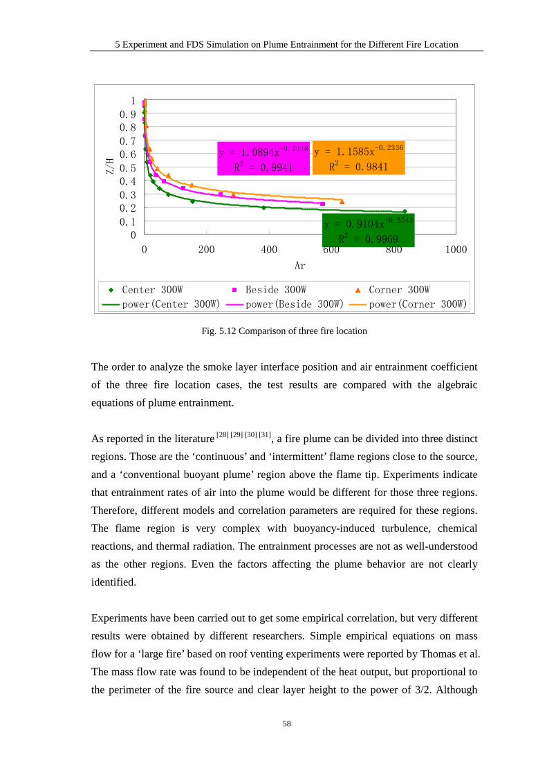
5 Experiment and FDS Simulation on Plume Entrainment for the Different Fire Location
58
y = 0.9104x-0.2543
R2 = 0.9969
y = 1.0894x-0.2448
R2 = 0.9941
y = 1.1585x-0.2336
R2 = 0.9841
00.1
0.20.3
0.40.5
0.60.7
0.80.9
1
0 200 400 600 800 1000
Ar
Z/H
Center 300W Beside 300W Corner 300W
power(Center 300W) power(Beside 300W) power(Corner 300W)
Fig. 5.12 Comparison of three fire location
The order to analyze the smoke layer interface position and air entrainment coefficient
of the three fire location cases, the test results are compared with the algebraic
equations of plume entrainment.
As reported in the literature [28] [29] [30] [31], a fire plume can be divided into three distinct
regions. Those are the ‘continuous’ and ‘intermittent’ flame regions close to the source,
and a ‘conventional buoyant plume’ region above the flame tip. Experiments indicate
that entrainment rates of air into the plume would be different for those three regions.
Therefore, different models and correlation parameters are required for these regions.
The flame region is very complex with buoyancy-induced turbulence, chemical
reactions, and thermal radiation. The entrainment processes are not as well-understood
as the other regions. Even the factors affecting the plume behavior are not clearly
identified.
Experiments have been carried out to get some empirical correlation, but very different
results were obtained by different researchers. Simple empirical equations on mass
flow for a ‘large fire’ based on roof venting experiments were reported by Thomas et al.
The mass flow rate was found to be independent of the heat output, but proportional to
the perimeter of the fire source and clear layer height to the power of 3/2. Although

5 Experiment and FDS Simulation on Plume Entrainment for the Different Fire Location
59
there is little theoretical justification for the ‘large fire’ equation, it was validated to be
consistent with existing experimental data by Hinkley [32]. This equation has the same
form as that by Zukoski et al. on the mass flow rate in the continuous flame region.
Only the thermal plume behavior is considered in this thesis. This is taken as a natural
convective problem. Four axisymmetric plume equations are commonly used to
calculate the mass flow rate m (in kg/s) at height Z (in meters) above a fire of
convective heat release rate Qc(in kW):
NFPA-92B equation [13]:
1 3 5 30.071 0.0018c cm Q Z Q= + (5.4)
for z>zf, where zf is the luminous flame height.
Equation by Zukoski : 1 3
1 3 5 3am c
p a
gm C Q Z
C T
ρ =
(5.5)
for z>zf, where zf depends on QD and the diameter of the pool fire D, and
0.21mC =
Equation by McCaffrey [33] [34]: 1.895
2 50.124 c
c
Zm Q
Q
=
(5.6)
for 2 5
0.2c
Z
Q>
Equation by Thomas et al. and Hinkley :
‘Small fire’ equation
( )1 3
5 31 20.153 1.5ca f
a p a
Q gm Z A
C Tρ
ρ
= +
(5.7a)
for 1 2fZ and fZ H≤ , 1 2
fZ H A d≤ + −
‘Large fire’ equation:
3 20.188m PZ= (5.7b)

5 Experiment and FDS Simulation on Plume Entrainment for the Different Fire Location
60
for ( )1 2 2fA H> − , ( )fZ H d> − and ( )Z H d≤ −
where aρ , Cp, and Ta are the density, specific heat, and temperature of the ambient air,
H is the ceiling height, P is the perimeter of the fire, d is the depth of the layer of hot
gas beneath the ceiling, and Af is the areas of the fire.
The equilibrium smoke layer interface position can be estimated for a particular heat
release rate and exhaust rate using the test data in experiment.
The basic principle of such an estimate is based on a statement of conservation of mass
applied to the upper smoke layer:
outm m= (5.8)
Volumetric smoke exhaust from the upper layer is:
out sm Veρ= (5.9)
Where
Ve--volumetric flow rate of exhaust gases (m3/s);
ρs--density of smoke exhaust (kg/m3), determined based on the ideal gas law as:
353s
sTρ = (5.10)
Where
Ts--temperature of exhaust smoke()
The temperature of the exhaust smoke was tested in the experiment.
The experimental results on a mass flow rate of the center fire case are shown in Fig.
5.13. The results predicted by the existing three axisymmetric plume equations are also
shown in the Figures.
It is observed that experiment predicted results on the mass flow rate agreed well with
the equations listed in NFPA-92B, the equation reported by Zukoski. The results
deviated from the equation due to McCaffrey. Note that this equation described the
induced behavior of the strong plume near the flame tip with turbulent effects. Higher
entrainment rates resulted due to turbulences.

5 Experiment and FDS Simulation on Plume Entrainment for the Different Fire Location
61
0.0
0.1
0.2
0.3
0.4
0.5
0.6
0.0 0.5 1.0 1.5 2.0 2.5 3.0 3.5
Z5/3
m/Q
c1/3
center 300W center 500W NFPA 92B equation
Zukisko equation McCaffrey equation
Fig. 5.13 Variation of mass flow rate with height
The experimental results on a mass flow rate of the three different fire location cases
are shown in Fig. 5.14.
y = 0.0453x - 7E-06
y = 0.0707x + 0.0014
0.0
0.1
0.1
0.2
0.2
0.3
0.0 0.5 1.0 1.5 2.0 2.5 3.0 3.5
Z5/3
m/Q
c1
/3
beside 300W beside 500W center 300W line(beside 500W) line(center 300W)
y = 0.0376x + 0.0011
y = 0.0707x + 0.0014
0.0
0.1
0.1
0.2
0.2
0.3
0.0 0.5 1.0 1.5 2.0 2.5 3.0 3.5
Z5/3
m/Q
c1/
3
conner 300W conner 500W center 300W line(conner 500W) line(300 W)
Fire located near to the wall Fire located near to the corner
Fig. 5.14 Comparison of Entrainment Coefficients
It is obvious that the plume entrainment coefficients are about 0.0707, 0.0478, and
0.0376 for the fire located in the center, near to the wall and near to the corner
respectively. It shows that the flow rate is 64% of the flow in a free central plume if the
fire is located near to the wall, and the flow rate is 48% of the flow in a free central
plume if the fire is located near to the corner.

6 Experiment and FDS Simulation on Balcony Plume
62
6 Experiment and FDS Simulation on Balcony Plume
In order to study the smoke flowing from a fire in a communicating space to atrium and smoke flowing from a fire in the atrium to the communicating space, the one half of the test compartment was used as communicating and divided into four parts in vertical direction by three clapboard as shown Fig. 6.1.
Fig. 6.1 Test compartment with communicating compartment
The communicating space dimension and thermocouples were shown as Fig. 6.2. There are four trees of thermocouple. A set of experiments that fire put on the floor were done. Fire location on the floor was shown as Fig. 6.3 and Table 6.1.
Table 6.1 Fire location
case X(mm) Y(mm)
AA 668 668
AB 85 85
AC 668 85
AD 668 1001
AE 668 1250
AF 85 1250

6 Experiment and FDS Simulation on Balcony Plume
63
107
x
1251335
F117
z 4
16
195
1
6 20
2
763
4343
2060
360
360
tree4
tree3 83
9
23tree1
448
43
(a)
y
11
1251335
380
F1
254
12
380
z
254
478
14
13
380
380
403
2060
160
15
380
160
tree2
447
224
tree1
(b)
tree3
y
x
1335
1335tree1 tree4
tree2
(c)
AD
AE
inlet
ground
AF
inlet
ABy
x
AA
AC
balcony
Fig. 6.2 Model dimension and thermocouple Fig. 6.3 Fire location on the floor
6.1 Smoke Movement from Atrium to Communicating Space
Smoke experiments with heat release rate 300W were done that fire put on the three different location of the atrium floor as shown in Fig. 6.3. The smoke exhaust rate and inlet air supply rate were designed in order to get a steady smoke layer height. The inlet air supply rate and smoke exhaust conditions were summarized in Table 6.2.
All dimension in mm

6 Experiment and FDS Simulation on Balcony Plume
64
Table 6.2 Inlet air supply rate and smoke exhaust rate in the experiment
case Inlet air supply
rate(m3/s)
Inlet air
velocity
(m/s)
Smoke exhaust
rate (m3/h)
Smoke exhaust
velocity
(m/s)
1 0.006 0.031 22.9 0.811
2 0.009 0.044 32.6 1.154
3 0.012 0.060 44.2 1.564
4 0.016 0.079 57.8 2.046
5 0.020 0.097 71.2 2.517
6 0.025 0.122 89.8 3.178
7 0.030 0.147 108.2 3.828
8 0.044 0.215 157.9 5.585
9 0.058 0.283 207.6 7.342
10 0.071 0.350 257.3 9.099
11 0.085 0.418 307.0 10.856
12 0.099 0.486 356.6 12.614
The fire placed in the center of floor that is case AA, fire near to the communicating space, case AB fire in the corner of atrium, case AC fire beside the wall in the atrium. At the test beginning the inlet and exhaust fans and the smoke box were opened.
Case AA
Case AB

6 Experiment and FDS Simulation on Balcony Plume
65
Case AC
Air supply rate 0.03 m3/s
Smoke exhaust rate 108.2 m3/h.
Fig. 6.4 Experimental smoke layer height recorded by video
For the case AA, at the test beginning the smoke plume quickly rose up to the ceiling and the plume spread horizontally and down, and meanwhile some of them spread into the second and third communicating space in the smoke move up process. Eventually formed steady smoke depth in atrium and then stopped at a certain height in several minutes. Meantime some smoke spread in the communicating space. Even if smoke exhaust rate was very larger and smoke layer height in atrium was also high, but there was smoke spread into the second communicating space as shown in Fig. 6.4. That is the fire close to the communicating space so smoke is easy to spread into the communicating space in the process of smoke move up. For the fire located in the corner or near the wall of the atrium that is case AB and AC, smoke move up to the ceiling and down, and spread into the communicating space. But steady smoke layer height both in the atrium and the communicating space is the same as shown in Fig. 6.4. During the test, the inlet air temperature, smoke exhaust temperature and smoke layer height in atrium were measured. The tested inlet air temperature, smoke temperature, smoke layer height, and Archimedes number for the case AA, AB and AC are shown in Table 6.3, Table 6.4 and Table 6.5 respectively. The smoke layer height in the tables is the smoke height in the atrium of the model. The dimensionless smoker layer height vs. Archimedes number and inlet air volumetric
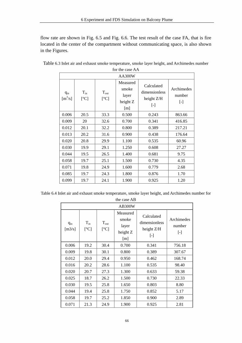
6 Experiment and FDS Simulation on Balcony Plume
66
flow rate are shown in Fig. 6.5 and Fig. 6.6. The test result of the case FA, that is fire located in the center of the compartment without communicating space, is also shown in the Figures.
Table 6.3 Inlet air and exhaust smoke temperature, smoke layer height, and Archimedes number
for the case AA
AA300W
qin
[m3/s]
Tin
[°C]
Tout
[°C]
Measured
smoke
layer
height Z
[m]
Calculated
dimensionless
height Z/H
[-]
Archimedes
number
[-]
0.006 20.5 33.3 0.500 0.243 863.66
0.009 20 32.6 0.700 0.341 416.85
0.012 20.1 32.2 0.800 0.389 217.21
0.013 20.2 31.6 0.900 0.438 176.64
0.020 20.8 29.9 1.100 0.535 60.96
0.030 19.9 29.1 1.250 0.608 27.27
0.044 19.5 26.5 1.400 0.681 9.75
0.058 19.7 25.1 1.500 0.730 4.35
0.071 19.8 24.9 1.600 0.779 2.68
0.085 19.7 24.3 1.800 0.876 1.70
0.099 19.7 24.1 1.900 0.925 1.20
Table 6.4 Inlet air and exhaust smoke temperature, smoke layer height, and Archimedes number for
the case AB
AB300W
qin
[m3/s]
Tin
[°C]
Tout
[°C]
Measured
smoke
layer
height Z
[m]
Calculated
dimensionless
height Z/H
[-]
Archimedes
number
[-]
0.006 19.2 30.4 0.700 0.341 756.18
0.009 19.8 30.1 0.800 0.389 307.67
0.012 20.0 29.4 0.950 0.462 168.74
0.016 20.2 28.6 1.100 0.535 98.40
0.020 20.7 27.3 1.300 0.633 59.38
0.025 18.7 26.2 1.500 0.730 22.33
0.030 19.5 25.8 1.650 0.803 8.80
0.044 19.4 25.8 1.750 0.852 5.17
0.058 19.7 25.2 1.850 0.900 2.89
0.071 21.3 24.9 1.900 0.925 2.81

6 Experiment and FDS Simulation on Balcony Plume
67
0.085 - - 2.000 0.973 -
0.099 - - - - -
Table 6.5 Inlet air and exhaust smoke temperature, smoke layer height, and Archimedes number for
the case AC
AC300W
qin
[m3/s]
Tin
[°C]
Tout
[°C]
Measured
smoke
layer
height Z
[m]
Calculated
dimensionless
height Z/H
[-]
Archimedes
number
[-]
0.006 20.3 31.3 0.600 0.292 607.65
0.009 20.4 30.5 0.750 0.365 301.06
0.012 20.4 29.4 0.850 0.414 161.56
0.016 20.8 29.2 1.000 0.560 87.93
0.020 20.4 29.0 1.150 0.657 59.38
0.025 20.7 28.7 1.350 0.730 34.60
0.030 19.5 28.0 1.500 0.779 25.31
0.044 19.8 26.5 1.600 0.827 9.36
0.058 20.1 26.1 1.700 0.876 4.85
0.071 19.8 25.7 1.800 0.925 3.10
0.085 20.7 26.3 1.900 0.925 2.07
0.099 - - - - -
0.0
0.1
0.2
0.3
0.4
0.5
0.6
0.7
0.8
0.9
1.0
0 100 200 300 400 500 600 700 800 900
Ar
Z/H
AA AB AC FA power power power
Fig. 6.5 Dimensionless smoke layer height vs. Archimedes number

6 Experiment and FDS Simulation on Balcony Plume
68
0.0
0.1
0.2
0.3
0.4
0.5
0.6
0.7
0.8
0.9
1.0
0.00 0.01 0.02 0.03 0.04 0.05 0.06 0.07 0.08
q(m3/s)
Z/H
AA AB AC FA
Fig. 6.6 Dimensionless smoke layer height vs. air inlet supply rate
It is obvious that the smoke layer height for the case AA is lower than the case AB and case AC on the same air volumetric and smoke exhaust rate conditions. That is fire in the center of the compartment, the plume entrain the ambient air. If the fire (source) is located close to the wall, or in the corner formed by the intersection of two walls, the entrainment will be reduced compared to the entrainment in a center plume and the resulting restriction on the air entrainment will have a significant effect. Compare to the case FA that is the fire located in the center of the compartment, the smoke layer height is higher in the case AA. That is some of the smoke spread into the half of compartment with the balcony in the case AA.
6.2 Smoke Movement from Communicating Space to Atrium
6.2.1 Experiment Result
In order to study the balcony plume entrainment and the effect of fire location on entrainment coefficient, smoke experiments with heat release rate 300W were done that fire put on the three different location of the recessed ground level room as shown in Fig. 6.3. The fire placed in the center of the recessed ground level room is case AD, which is the fire located in the center of the communicating space. The case AE is the fire in the corner of the ground level communicating space, case AF is that the fire beside the wall in the ground level communicating space. At the test beginning the inlet and exhaust fans and the smoke box were opened. The smoke exhaust rate and inlet air supply rate were designed in order to get a steady smoke layer height. The inlet air supply rate and smoke exhaust conditions were summarized in Table 6.2.

6 Experiment and FDS Simulation on Balcony Plume
69
During the test, the inlet air temperature, smoke exhaust temperature and smoke layer height in the atrium were measured. The tested inlet air temperature, smoke temperature, smoke layer height, and Archimedes number for the case AD, AE and AF are shown in Table 6.6, Table 6.7 and Table 6.8 respectively. The smoke layer height Zp and Zb in the tables are the smoke height in the atrium of the model and the level space respectively as shown in Fig. 6.7.
Fire
Air inlet
Zp
H
Zbhb
Db
Smoke exhaust
Smoke
Ceiling
Fig. 6.7 Typical balcony plume
Table 6.6 Inlet air and exhaust smoke temperature, smoke layer height, and Archimedes number for
the case AD
AD300W
qin
[m3/s] vin[m/s]
Tin
[°C]
Tout
[°C]
Smoke
layer
height
Zp[m]
dimensionless
height Zp/H
Zb
[m] Zb/hb
Archimedes
number
0.006 0.031 21.0 29.4 0.400 0.195 0.400 0.524 567.14
0.009 0.044 21.2 29.6 0.500 0.243 0.450 0.590 277.90
0.012 0.060 21.4 29.4 0.550 0.268 0.460 0.603 143.61
0.016 0.079 21.3 29.2 0.600 0.292 0.460 0.603 82.69
0.020 0.097 21.3 29.0 0.650 0.316 0.470 0.616 53.17
0.025 0.122 21.8 28.7 0.750 0.365 0.480 0.629 29.85
0.030 0.147 20.6 25.7 0.800 0.389 0.500 0.655 15.19
0.044 0.215 20.7 25.7 0.850 0.414 0.500 0.655 6.98
0.058 0.283 20.9 25.5 0.900 0.438 0.500 0.655 3.72
0.071 0.350 21.1 25.3 0.950 0.462 0.500 0.655 2.21
0.085 0.418 21.2 25.2 1.000 0.487 0.500 0.655 1.48
0.099 0.486 21.3 24.9 1.050 0.511 0.500 0.655 0.98

6 Experiment and FDS Simulation on Balcony Plume
70
Table 6.7 Inlet air and exhaust smoke temperature, smoke layer height, and Archimedes number for
the case AE
AE300W
qin
[m3/s] vin[m/s]
Tin
[°C]
Tout
[°C]
Smoke
layer
height
Zp[m]
dimensionless
height Zp/H
Zb
[m] Zb/hb
Archimedes
number
0.006 0.031 20.8 27.2 0.500 0.243 0.500 0.655 432.10
0.009 0.044 20.7 27.5 0.600 0.292 0.550 0.721 224.96
0.012 0.060 21.1 27.8 0.650 0.316 0.580 0.760 120.27
0.016 0.079 21.2 27.9 0.700 0.341 0.600 0.786 70.13
0.020 0.097 21.6 27.8 0.750 0.365 0.600 0.786 42.81
0.025 0.122 21.9 27.6 0.800 0.389 0.600 0.786 24.66
0.030 0.147 22.2 28.2 0.850 0.414 0.600 0.786 17.86
0.044 0.215 21.9 27.9 0.900 0.438 0.600 0.786 8.38
0.058 0.283 21.9 27.0 0.950 0.462 0.600 0.786 4.12
0.071 0.350 22.1 26.4 1.000 0.487 0.600 0.786 2.26
0.085 0.418 22.3 25.7 1.050 0.511 0.600 0.786 1.26
0.099 0.486 22.0 25.0 1.100 0.535 0.600 0.786 0.82
Table 6.8 Inlet air and exhaust smoke temperature, smoke layer height, and Archimedes number for
the case AF
AF300W
qin
[m3/s] vin[m/s]
Tin
[°C]
Tout
[°C]
Smoke
layer
height
Zp[m]
dimensionless
height Zp/H
Zb
[m] Zb/hb
Archimedes
number
0.006 0.031 20.8 27.6 0.550 0.268 0.550 0.721 459.11
0.009 0.044 21.2 27.6 0.650 0.316 0.580 0.760 211.73
0.012 0.060 21.0 28.2 0.700 0.341 0.580 0.760 129.25
0.016 0.079 21.4 28.0 0.750 0.365 0.600 0.786 69.09
0.020 0.097 21.3 29.2 0.800 0.389 0.600 0.786 54.55
0.025 0.122 21.6 28.2 0.850 0.414 0.600 0.786 28.55
0.030 0.147 20.9 27.1 0.900 0.438 0.600 0.786 18.46
0.044 0.215 21.4 26.8 0.950 0.462 0.600 0.786 7.54
0.058 0.283 21.3 26.5 1.000 0.487 0.600 0.786 4.20
0.071 0.350 21.5 26.2 1.050 0.511 0.620 0.813 2.47
0.085 0.418 21.4 25.9 1.100 0.535 0.650 0.852 1.66
0.099 0.486 21.7 26.0 1.150 0.560 0.650 0.852 1.18
The dimensionless smoker layer height vs. Archimedes number and inlet air volumetric

6 Experiment and FDS Simulation on Balcony Plume
71
flow rate are shown in Fig. 6.8 and Fig. 6.9 for the case AD AE and AF.
0.0
0.1
0.2
0.3
0.4
0.5
0.6
0.7
0.8
0.9
1.0
0 100 200 300 400 500 600
Ar
Z/H
AD AE AF power power power
Fig. 6.8 Dimensionless smoke layer height vs. Archimedes number
0.0
0.1
0.2
0.3
0.4
0.5
0.6
0.00 0.01 0.02 0.03 0.04 0.05 0.06 0.07 0.08
q(m3/s)
Z/H
AD AE AF
Fig. 6.9 Dimensionless smoke layer height vs. air inlet supply rate
It is obvious that at the same Archimedes number and air supply rate the smoke layer height is the lowest for the case AD. It is that the fire at the center of the communicating space it is an axisymmetric plume and air is entrained around all sides of the plume. In case AE and AF the fire placed near a wall or the corner of the wall and their entrainment are restricted.
6.2.2 FDS Simulation
To obtain more information about the smoke layer on the smoke exhaust condition,

6 Experiment and FDS Simulation on Balcony Plume
72
CFD simulations were finished by adopting large eddy simulation (LES) program. In the simulations, the smoke movement was simulated by a steady fire, the initial temperature and air inlet volume and smoke exhaust rate were set according to the measurements in the experiments. Table 6.9, Table 6.10 and Table 6.11 show the result for the 300W fire simulated by FDS. Table 6.9 Inlet air and exhaust smoke temperature, smoke layer height, and Archimedes number for
the case AD by FDS
AD300W
qin
[m3/s] vin[m/s]
Tin
[°C]
Tout
[°C]
Smoke
layer
height
Zp[m]
dimensionless
height Zp/H
Zb
[m] Zb/hb
Archimedes
number
0.012 0.060 20.0 23.5 0.584 0.284 0.414 0.543 62.83
0.016 0.079 20.0 23.4 0.613 0.298 0.450 0.590 35.59
0.020 0.097 20.0 23.1 0.664 0.323 0.461 0.604 21.41
0.025 0.122 20.0 23.1 0.698 0.340 0.461 0.604 13.41
0.030 0.147 20.0 23.0 0.720 0.350 0.468 0.613 8.93
0.044 0.215 20.0 22.5 0.734 0.357 0.482 0.632 3.49
0.058 0.283 20.0 22.1 0.765 0.372 0.500 0.655 1.70
0.071 0.350 20.0 21.8 0.802 0.390 0.501 0.657 0.95
0.085 0.418 20.0 21.6 0.822 0.400 0.504 0.661 0.59
0.099 0.486 20.0 21.3 0.884 0.430 0.509 0.667 0.36
0.012 0.060 20.0 21.3 0.925 0.450 0.510 0.668 0.33
0.016 0.079 20.0 21.3 1.020 0.496 0.512 0.671 0.26
Table 6.10 Inlet air and exhaust smoke temperature, smoke layer height, and Archimedes number
for the case AE by FDS
AE300W
qin
[m3/s] vin[m/s]
Tin
[°C]
Tout
[°C]
Smoke
layer
height
Zp[m]
dimensionless
height Zp/H
Zb
[m] Zb/hb
Archimedes
number
0.012 0.060 20.0 24.5 0.597 0.291 0.503 0.659 80.78
0.016 0.079 20.0 24.4 0.638 0.310 0.578 0.758 46.06
0.020 0.097 20.0 24.3 0.661 0.322 0.623 0.817 29.69
0.025 0.122 20.0 24.2 0.706 0.344 0.635 0.832 18.17
0.030 0.147 20.0 23.8 0.725 0.353 0.583 0.764 11.31
0.044 0.215 20.0 23.7 0.769 0.374 0.567 0.743 5.17
0.058 0.283 20.0 23.6 0.777 0.378 0.597 0.782 2.91

6 Experiment and FDS Simulation on Balcony Plume
73
0.071 0.350 20.0 23.5 0.803 0.391 0.594 0.779 1.84
0.085 0.418 20.0 23.5 0.916 0.446 0.560 0.734 1.29
0.099 0.486 20.0 23.3 0.975 0.474 0.509 0.667 0.90
0.102 0.500 20.0 23.1 1.030 0.501 0.568 0.744 0.80
0.116 0.569 20.0 22.9 1.100 0.535 0.568 0.744 0.58
Table 6.11 Inlet air and exhaust smoke temperature, smoke layer height, and Archimedes number
for the case AF by FDS
AF300W
qin
[m3/s] vin[m/s]
Tin
[°C]
Tout
[°C]
Smoke
layer
height
Zp[m]
dimensionless
height Zp/H
Zb
[m] Zb/hb
Archimedes
number
0.012 0.060 20.0 23.2 0.627 0.305 0.565 0.740 57.44
0.016 0.079 20.0 23.0 0.653 0.318 0.632 0.828 30.36
0.020 0.097 20.0 22.9 0.685 0.333 0.637 0.835 20.02
0.025 0.122 20.0 22.9 0.715 0.348 0.653 0.856 12.11
0.030 0.147 20.0 22.8 0.755 0.367 0.617 0.809 8.04
0.044 0.215 20.0 22.7 0.760 0.370 0.627 0.822 2.65
0.058 0.283 20.0 21.9 0.821 0.400 0.652 0.855 1.53
0.071 0.350 20.0 21.9 0.886 0.431 0.653 0.856 0.79
0.085 0.418 20.0 21.5 0.933 0.454 0.657 0.861 0.55
0.099 0.486 20.0 21.5 1.060 0.516 0.597 0.782 0.41
0.102 0.500 20.0 21.3 1.100 0.535 0.607 0.796 0.33
0.116 0.569 20.0 21.2 1.180 0.574 0.615 0.806 0.24
Fig. 6.10 shows a comparison of smoke temperature profile at the center of the model (tree 1) between experimental and numerical temperature simulated by FDS for the case AD. The CFD simulation seems to over predict the temperature near the ceiling and shows a temperature gradient within hot layer, while the experimental data indicate that the temperature in the hot layer is uniform. Despite the difference in the temperature values between the simulation and experimental data, there is a good agreement between the experimental and numerical hot layer height in the compartment.
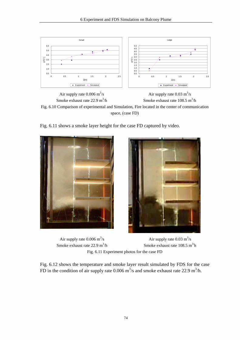
6 Experiment and FDS Simulation on Balcony Plume
74
Small
0.0
1.0
2.0
3.0
4.0
5.0
6.0
0 0.5 1 1.5 2 2.5
Z(m)
∆T
()
Experiment Simulated
Large
0.00.5
1.01.52.02.5
3.03.54.0
4.55.0
0 0.5 1 1.5 2 2.5
Z(m)
∆T
()
Experiment Simulated
Air supply rate 0.006 m3/s
Smoke exhaust rate 22.9 m3/h
Air supply rate 0.03 m3/s
Smoke exhaust rate 108.5 m3/h
Fig. 6.10 Comparison of experimental and Simulation, Fire located in the center of communication
space, (case FD)
Fig. 6.11 shows a smoke layer height for the case FD captured by video.
Air supply rate 0.006 m3/s
Smoke exhaust rate 22.9 m3/h
Air supply rate 0.03 m3/s
Smoke exhaust rate 108.5 m3/h
Fig. 6.11 Experiment photos for the case FD
Fig. 6.12 shows the temperature and smoke layer result simulated by FDS for the case FD in the condition of air supply rate 0.006 m3/s and smoke exhaust rate 22.9 m3/h.
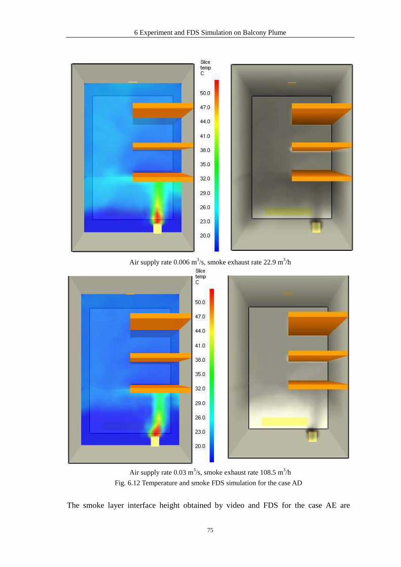
6 Experiment and FDS Simulation on Balcony Plume
75
Air supply rate 0.006 m3/s, smoke exhaust rate 22.9 m3/h
Air supply rate 0.03 m3/s, smoke exhaust rate 108.5 m3/h
Fig. 6.12 Temperature and smoke FDS simulation for the case AD
The smoke layer interface height obtained by video and FDS for the case AE are

6 Experiment and FDS Simulation on Balcony Plume
76
shown in Fig. 1 and Fig. 2 in Appendix B.
The smoke layer interface height obtained by video and FDS simulation for the case
AF are shown in Fig. 3 and Fig. 4 in Appendix B.
6.3 Balcony Plume Entrainment
Different geometrical arrangements of fire inside a building could lead to different entrainment, and hence different plume expressions. Basically, three types of plumes are commonly encountered in designing smoke control system. Axisymmetric plumes: for a fire placed at the center of a big hall, ambient air is entrained from all sides along the height of the plume. The research on this section sees section 5 in this report. Balcony spill plumes: for a fire in a shop adjacent to the atrium, scenarios with balcony spill plumes involve smoke rising above the fire; reaching the ceiling, balcony, or other significant horizontal projection; then traveling horizontally toward the edges of the balcony. Door plumes: plumes issuing from openings, such as doors and windows, into a large-volume, open space. A typical balcony spill plume due to a fire located at a recessed ground level room is shown in Fig. 6.7. Hot smoke generated by the fire rises up to the ceiling of the room, forms an elevated layer of thickness Db under the wide balcony, spills into the atrium and then rises due to buoyancy. More ambient air is entrained into it. The estimation of the air entrainment rate is very important for designing the smoke control system in an atrium. Entrainment into the smoke flows at the balcony edge and into the rising plume might be calculated by plume equation. For example BRE spill plume model and plume model of Thomas detailed descriptions of this method can be found in the literature. Plume model of Thomas Plume model of Thomas was taken as a ‘far plume’ rising from a line source of zero thickness some distance below the void edge. A relatively simple plume equation with virtual source correction on mass flow rate mp at height Zp can be given as
( ) ( ) 3/23/12 222.0
158.0
∆++∆+
=
W
ZZ
TC
WgQm p
papg
cgp ρ
ρ (6.1)
Where ∆ is the empirical height of the virtual source below the balcony, Zp is the height

6 Experiment and FDS Simulation on Balcony Plume
77
above the balcony, and W is the width of the plume as it spills under the balcony. For small Zp/W, the main term is consistent with Lee and Emmons model [28]. The results would be reduced to the conventional point source plume theory for Zp>>W. Spill plume model of Poreh et al [36] By assuming that the entrainment into the curved section of the spilling plume is approximately equal to the entrainment into a vertical free plume rising through the same height, a very simple model was proposed by Poreh et al. for calculating the mass flux of free plumes in relatively wide atria. The mass entrainment rate mp of the spill plume at Zp is given by:
( )1 3p b c p bm m CQ Z D= + + (6.2)
Where, mb is the mass flow of gases beneath the balcony, Db is the depth of the smoke layer beneath the balcony, and C is a constant, which is defined as:
2 310.3 m aC C Wρ= (6.3)
Where, Cm1 is the dimensionless entrainment coefficient, determined experimentally to be 0.44 for a free plume. Spill plume model of Thomas et al. [37] Applying dimensional analysis without taking the assumptions on similarity or constant entrainment coefficient into account, an entrainment coefficient of 0.11 was deduced, rather than assumed for the larger hood. The value is consistent with the more recent studies of line plumes. The mass entrainment rate mp at Zp can be estimated by:
( )2 1 31.20 0.159 ( ) 0.0027p b p c cm m Z Q W Q= + (6.4)
Taking the entrainment into both free ends ∆mp as:
( )2 1 31.20 0.159 ( ) 0.0027p b p c cm m Z Q W Q∆ = + (6.5)
The total entrainment rate becomes:
( )1 32 1 31.2 0.16 ( ) 0.0027 0.09p b p c c p cm m Z Q W Q Z Q W= + + (6.6)
NFPA spill plume equation Based on the interpretation of the small-scale experiments by Morgan and Marshall, a good linear relationship between mp and Zb was found by Law [38]. The mass production rate can be expressed as:
( )2 1 30.36( ) 0.25p b bm QW Z h= + (6.7)
Where, hb is the height of the balcony, Zb is the height above the balcony (Zb=Zp-hb) and Q is the heat release of the fire.

6 Experiment and FDS Simulation on Balcony Plume
78
Although all these models were based on the same set of experimental data, different mass flow equations were derived. The difference is due to the method for estimating the air entrainment into the plume while hot smoke is spilling underneath a balcony edge and rising into the large atrium void. Further studies of these models are needed. Three cases, AD, AE and AF, that is a fire located at the center, beside the wall and the corner of a recessed ground level room, as shown in Fig. 6.3, were considered for studying the mass entrainment rate of the balcony spill plumes. The experiment was designed to test the smoke layer height on the steady fire and smoke exhaust rate condition. The equilibrium smoke layer interface position can be estimated for a particular heat release rate and exhaust rate using the test data in experiment. The basic principle of such an estimate is based on a statement of conservation of mass applied to the upper smoke layer. The mass entrainment rate is obtained by the following formula:
outm m= (6.8)
Where, m is the mass flow rate of the balcony spill plume. Volumetric smoke exhaust from the upper layer is:
out sm Veρ= (6.9)
Where Ve--volumetric flow rate of exhaust gases (m3/s); ρs--density of smoke exhaust (kg/m3), determined based on the ideal gas law as:
353s
sTρ = (6.10)
Where Ts--temperature of exhaust smoke ( ) . The temperature of the exhaust smoke and volumetric flow rate of exhaust gases were tested in the experiment. FDS simulation and experiment results of the case AD, AE, and AF with the heat release 300W are compared with those by different spill plume models shown in Fig. 6.13. It is obvious that a linear relationship between the numerical mp and Zp can be observed. The coefficient of the mass flow rate of the balcony plume is between 0.342 and 0.468. A good agreement is found between the results of CFD simulation and experiment in this report and those predicted by the NFPA plume equations. Larger discrepancies among the simulation, experiment results and those estimated by the Thomas equation were found.

6 Experiment and FDS Simulation on Balcony Plume
79
The possible explanations are:
NFPA equation was derived from experimental data. The equation of Thomas was
derived from two-dimensional plumes. The plume might not be two-dimensional and
there might be end entrainment.
0.00
0.05
0.10
0.15
0.20
0.25
0.30
0.5 0.6 0.7 0.8 0.9 1.0 1.1 1.2 1.3
Zp
mp/
(QcW
2 )1/3
AD300W FDS AD300W Experiment AE300W FDS
AE300W Experiment AF300W FDS AF300W Experiment
Thomas NFPA
Fig. 6.13 Relationship between Zp and mp/(QcW
2)1/3 in three cases for the FDS simulation and
experiment (300W fire)
The smoke temperature and smoke layer height tested in the experiment and simulated
by FDS for the 500w fire are shown in Table 6.12 and Table 6.13.
FDS simulation and experiment results of the case AD with heat release 500W are compared with those by different spill plume models shown in Fig. 6.14. It is obvious that a good agreement is found between the 500W fire results and those predicted by the NFPA plume equations.
Fig. 6.15 shows a comparison of CFD and experiment results for case AD, AE, and AF
are compared with that by spill plume models in NFPA. It is obvious that the balcony
plume entrainment coefficient is independent of the fire location. And compared with
the NFPA model, the error range of the results from the experiment and FDS
simulation data in this report is between -0.08 and 0.05. The balcony equation in NFPA
would give good predictions on the mass flow rate.

6 Experiment and FDS Simulation on Balcony Plume
80
Table 6.12 Inlet air and exhaust smoke temperature, smoke layer height, and Archimedes number
for the case AD 500W
AD500W
qin
[m3/s] vin[m/s]
Tin
[°C]
Tout
[°C]
Smoke
layer
height
Zp[m]
dimensionless
height Zp/H
Zb
[m] Zb/hb
Archimedes
number
0.006 0.031 21.0 30.7 0.450 0.219 0.400 0.524 654.91
0.009 0.044 21.3 33.7 0.500 0.243 0.400 0.524 410.23
0.012 0.060 21.3 33.7 0.550 0.268 0.400 0.524 222.59
0.016 0.079 21.5 34.6 0.600 0.292 0.400 0.524 137.13
0.020 0.097 21.8 32.4 0.650 0.316 0.400 0.524 73.19
0.025 0.122 21.8 31.8 0.700 0.341 0.400 0.524 43.26
0.030 0.147 21.1 27.5 0.750 0.365 0.400 0.524 19.06
0.044 0.215 21.4 27.5 0.800 0.389 0.500 0.655 8.52
0.058 0.283 21.2 27.2 0.850 0.414 0.500 0.655 4.85
0.071 0.350 21.5 27.0 0.900 0.438 0.500 0.655 2.89
0.085 0.418 21.4 26.4 0.950 0.462 0.500 0.655 1.85
0.099 0.486 21.7 26.0 1.000 0.487 0.500 0.655 1.18
Table 6.13 Inlet air and exhaust smoke temperature, smoke layer height, and Archimedes number
for the case AD 500W by FDS
AD500W
qin
[m3/s] vin[m/s]
Tin
[°C]
Tout
[°C]
Smoke
layer
height
Zp[m]
dimensionless
height Zp/H
Zb
[m] Zb/hb
Archimedes
number
0.012 0.060 20.0 25.8 0.579 0.282 0.414 0.543 104.12
0.016 0.079 20.0 25.6 0.591 0.288 0.450 0.590 58.62
0.020 0.097 20.0 25.0 0.610 0.297 0.461 0.604 34.52
0.025 0.122 20.0 24.8 0.685 0.333 0.461 0.604 20.76
0.030 0.147 20.0 24.7 0.697 0.339 0.468 0.613 13.99
0.044 0.215 20.0 24.6 0.739 0.360 0.482 0.632 6.43
0.058 0.283 20.0 24.0 0.781 0.380 0.500 0.655 3.23
0.071 0.350 20.0 23.9 0.800 0.389 0.501 0.657 2.05
0.085 0.418 20.0 23.2 0.819 0.399 0.504 0.661 1.18
0.099 0.486 20.0 22.5 0.854 0.416 0.509 0.667 0.68
0.012 0.060 20.0 22.3 0.891 0.434 0.510 0.668 0.59
0.016 0.079 20.0 21.9 0.963 0.469 0.512 0.671 0.38
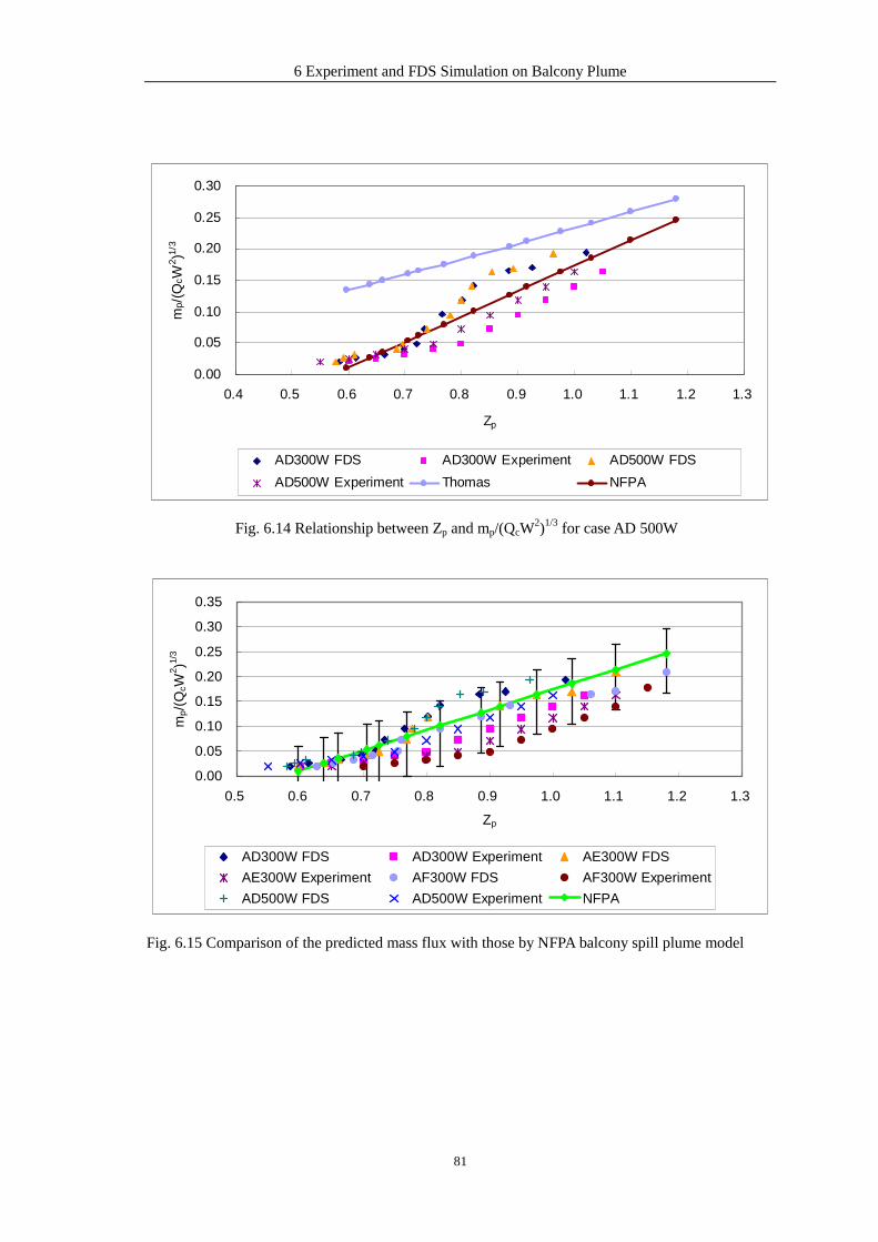
6 Experiment and FDS Simulation on Balcony Plume
81
0.00
0.05
0.10
0.15
0.20
0.25
0.30
0.4 0.5 0.6 0.7 0.8 0.9 1.0 1.1 1.2 1.3
Zp
mp/
(QcW
2 )1/3
AD300W FDS AD300W Experiment AD500W FDS
AD500W Experiment Thomas NFPA
Fig. 6.14 Relationship between Zp and mp/(QcW2)1/3 for case AD 500W
0.00
0.05
0.10
0.15
0.20
0.25
0.30
0.35
0.5 0.6 0.7 0.8 0.9 1.0 1.1 1.2 1.3
Zp
mp/
(QcW
2 )1/3
AD300W FDS AD300W Experiment AE300W FDS
AE300W Experiment AF300W FDS AF300W Experiment
AD500W FDS AD500W Experiment NFPA
Fig. 6.15 Comparison of the predicted mass flux with those by NFPA balcony spill plume model

7 Experiment and FDS Simulation on Smoke Movement in Large Space Building with Sloping Floor
82
7 Experiment and FDS Simulation on Smoke Movement in Large Space Building with Sloping Floor
As many large space buildings such as cinema, sports arenas containing the sloping
floor are designed to meet the function and aesthetic requirement. In this chapter,
smoke movement in this kind of building is discussed.
The scheme of the compartment with sloping floor is shown in Fig. 7.1. The half of
floor is designed as the sloping floor shown in Fig. 7.2. The sloping floor was made of
the filter.
1335
1335
inlet
2055
fire
inlet
outlet
D=100
A
outlet
1335
2055
inlet
fire
1335
inlet
fire
D=100
B
Fig. 7.1 Scheme of model with Sloping Floor
All dimension in mm

7 Experiment and FDS Simulation on Smoke Movement in Large Space Building with Sloping Floor
83
Fig. 7.2 Sloping floor
In the test compartment there were three thermocouple trees. A set of 6 thermocouples
with 380mm intervals was vertically placed at the center of the compartment over the
fire source. A second set of 7 thermocouples with 380mm intervals was also vertically
placed at the corner of the compartment, and a third set of 3 thermocouples with
380mm, 155mm intervals was also vertically placed at the other corner of the
compartment, as shown in Fig. 7.3.
433
235
235
235
334
235
B
B
433 433
433
24
18
173
16 20
19
21
923
20
380
y
x
Inle
t
Inle
t
Signaturforklaring
All demension in mm
Thermocouple
380
155
433433235 235
380
380
380
380
2 8 15
1 7 14
6 13
5 12
4 11
24
22
17 10
3 16
20
220
155
923
y
x
Plane B-B
a) b)
Fig. 7.3 Thermocouple in the sloping floor space

7 Experiment and FDS Simulation on Smoke Movement in Large Space Building with Sloping Floor
84
Three degree sloping floor are designed as shown in Fig. 7.4.
1335
1335
668
668
C
C
y
x
Inle
t
Inle
t
Plane Significance
incline plane
All demension i n mm
fire
1335
2055
y
x
plane C-C
Fig. 7.4 Scheme of the sloping floor with different degree
7.1 Experiment Condition
The series of experiments were conducted. The experimental schemes for the different
degrees of the sloping floor are shown in Table 7.1. For the 20 degree sloping floor
five cases have been designed to study the fire location and other heat source on smoke
movement. One of them was that there was a cable with heat source 100W on the
sloping floor, and the inlet air was induced from the opening in the two side of the
model as shown in Fig. 7.1b. The other two cases were fire heat power with 300W and
500W. And the inlet air from the opening in the two side of the model was induced into
the compartment through the sloping floor as shown in Fig. 7.1a.
Table 7.1 Degree of sloping floor and experiment scheme
case angle location heat cables Air supply
SA 20 floor 300 0 slope
SB 50 floor 300 0 slope
SC 72 floor 300 0 slope
SD 20 floor 300 100 slope
SE 20 slope 300 0 sides
SF 20 slope 300 100 sides

7 Experiment and FDS Simulation on Smoke Movement in Large Space Building with Sloping Floor
85
In the experiment beginning the fire source produced smoke and the smoke plume rose
quickly up to the ceiling and then the plume spread horizontally and down, eventually
formed steady smoke depth and then stopped at a certain height in several minutes.
During the test, the inlet air temperature, smoke exhaust temperature and smoke layer
height were measured.
7.2 Experimental Result of the Sloping Floor with Different Angle
On the condition of 300W fire in the center of the model, three sets of experiment were
conducted for the different angle sloping floor, as shown in Table 7.1. The tested inlet
air temperature, smoke temperature, smoke layer height, and Archimedes number for
the sloping floor are shown in Table 7.1.
The smoker layer height vs. Archimedes number and inlet air volumetric flow rate are
shown in Table 7.2, Table 7.3 and Table 7.4. The result from the center fire without
sloping floor is also shown in the Figure. It is obvious that smoke layer height of the
case SC is the lowest on the same inlet air supply rate. That is that the compartment
volume is smaller as the degree sloping floor is bigger. But the discrepancy is not very
distinct. The same dimensionless smoke layer height the Archimedes number is bigger
for the case SC, as the inlet areas is bigger and then the inlet air velocity is smaller.
Table 7.2 The experiment result for the 20 degree sloping floor (300W center fire)
Case qin
(m3/s)
Inlet air
velocity
(m/s)
Smoke
exhaust
rate
(m3/h)
Layer
heighZ(m) Tin/ Tout/
Dimensionless
height Z/H
Archimedes
number
SA1 0.006 0.011 22.9 0.350 18.4 25.7 0.170 4115
SA2 0.009 0.016 32.6 0.400 18.5 25.4 0.195 1907
SA3 0.012 0.021 44.2 0.500 18.9 25.3 0.243 960
SA4 0.016 0.027 56.3 0.600 19 25.2 0.292 571
SA5 0.030 0.053 108.5 0.900 19.6 24.8 0.438 129
SA6 0.037 0.065 133.4 0.950 19.9 24.5 0.462 75
SA7 0.044 0.077 158.1 1.150 19.1 24.2 0.560 59
SA8 0.058 0.101 207.8 1.300 19.1 23.1 0.633 27
SA9 0.071 0.126 257.4 1.400 19.3 22.8 0.681 15

7 Experiment and FDS Simulation on Smoke Movement in Large Space Building with Sloping Floor
86
SA10 0.085 0.150 307.1 1.450 19.6 23.2 0.706 11
SA11 0.099 0.174 356.7 1.650 19.7 21.5 0.803 4
Table 7.3 The experiment result for the 50 degree sloping floor (300W center fire)
Case qin
(m3/s)
Inlet air
velocity
(m/s)
Smoke
exhaust
rate
(m3/h)
Layer
height
Z(m)
Tin/ Tout/ Dimensionless
height Z/H
Archimedes
number
SB1 0.006 0.008 22.9 0.450 19.0 28.3 0.219 9068
SB2 0.007 0.009 25.4 0.450 18.9 28.1 0.219 7431
SB3 0.009 0.012 32.6 0.500 19.0 27.1 0.243 3958
SB4 0.012 0.016 44.2 0.600 19.3 26.5 0.292 1909
SB5 0.016 0.021 56.3 0.700 19.3 26.0 0.341 1092
SB6 0.025 0.033 89.8 0.850 19.7 24.8 0.414 326
SB7 0.030 0.040 108.5 1.100 18.3 22.9 0.535 201
SB8 0.037 0.049 133.4 1.150 18.3 22.9 0.560 133
SB9 0.044 0.058 158.1 1.300 18.0 22.7 0.633 97
SB10 0.058 0.076 207.8 1.450 18.7 22.5 0.706 45
SB11 0.065 0.086 234.2 1.500 18.8 22.3 0.730 33
SB12 0.071 0.094 257.4 - - - - -
SB13 0.085 0.113 307.1 - - - - -
SB14 0.099 0.131 356.7 - - - - -
Table 7.4 The experiment result for the 72 degree sloping floor (300W center fire)
Case qin
(m3/s)
Inlet air
velocity
(m/s)
Smoke
exhaust
rate
(m3/h)
Layer
height
Z(m)
Tin/ Tout/ Dimensionless
height Z/H
Archimedes
number
SC1 0.006 0.004 22.9 0.400 18.4 27.1 0.195 40172
SC2 0.007 0.004 25.4 0.450 18.3 26.9 0.219 32137
SC3 0.009 0.005 32.6 0.500 18.5 26.5 0.243 20464
SC4 0.012 0.007 44.2 0.550 18.5 26.3 0.268 10826
SC5 0.016 0.009 56.3 0.600 19.0 26.3 0.292 6228
SC6 0.025 0.014 89.8 0.700 19.4 25.8 0.341 2145

7 Experiment and FDS Simulation on Smoke Movement in Large Space Building with Sloping Floor
87
SC7 0.030 0.017 108.5 0.850 17.5 24.1 0.414 1512
SC8 0.037 0.021 133.4 1.000 17.8 23.6 0.487 878
SC9 0.044 0.025 158.1 1.200 18.0 22.1 0.584 442
SC10 0.058 0.033 207.8 1.450 18.2 22.6 0.706 274
SC11 0.065 0.038 234.2 - - - - -
SC12 0.071 0.041 257.4 - - - - -
SC13 0.085 0.049 307.1 - - - - -
SC14 0.099 0.057 356.7 - - - - -
The dimensionless smoker layer height vs. Archimedes number and inlet air volumetric
flow rate are shown in Fig. 7.3 and Fig. 7.4. The result from the center fire without
sloping floor (case FA) is also shown in the Figure. It is obvious that smoke layer
height of the case SC is the lowest on the same inlet air supply rate. That is that the
compartment volume is smaller as the degree sloping floor is bigger. But the
discrepancy is not very distinct. At the same dimensionless smoke layer height the
Archimedes number is larger for the case SC, as the inlet areas is larger and then the
inlet air velocity is smaller.
The relationship between Archimedes number and dimensionless smoke layer height
for the 20, 50, and 72 degree sloping floor can be described as equation (7.1), (7.2) and
(7.3) respectively.
0.2371.2879z
ArH
−= (7.1)
0.22991.6993z
ArH
−= (7.2)
-0.2378Z = 2.4378Ar
H (7.3)

7 Experiment and FDS Simulation on Smoke Movement in Large Space Building with Sloping Floor
88
0.0
0.1
0.2
0.3
0.4
0.5
0.6
0.7
0.8
0.9
1.0
0 200 400 600 800 1000 1200 1400 1600 1800 2000
Ar
Z/H
SA SB SC FA power power power power
Fig. 7.3 Dimensionless smoke layer height Vs. Archimedes number
0.0
0.1
0.2
0.3
0.4
0.5
0.6
0.7
0.8
0.9
1.0
0.00 0.01 0.02 0.03 0.04 0.05 0.06 0.07 0.08
q(m3/s)
Z/H
SA SB SC FA
Fig. 7.4 Dimensionless smoker layer height vs. inlet air flow rate for the different degree sloping
floor (300W)
The photos of the smoke layer interface height obtained by the video for the sloping
floor are shown in Fig. 1 in Appendix C.
7.3 Experimental Result of the Sloping Floor with 20 Degree
1) Fire on the center of the floor

7 Experiment and FDS Simulation on Smoke Movement in Large Space Building with Sloping Floor
89
In order to analyze the effect of other heat source on smoke movement, the fire was
located on the center of the model and 100W cable was put on the sloping as case SD.
The tested inlet air temperature, smoke temperature, smoke layer height, and
Archimedes number for the heat source on sloping floor and fire in the center of
compartment are shown in Table 7.5.
Table 7.5 The experiment result for the 20 degree sloping floor (300W floor fire, 100W cable)
Case qin
(m3/s)
Inlet air
velocity
(m/s)
Smoke
exhaust
rate
(m3/h)
Layer
height
Z(m)
Tin/ Tout/ Dimensionless
height Z/H
Archimedes
number
SD1 0.006 0.011 22.9 0.001 20.9 29.2 0.000 4679
SD2 0.009 0.016 32.6 0.100 21.2 30.9 0.049 2681
SD3 0.012 0.021 44.2 0.200 21.3 30.5 0.097 1380
SD4 0.016 0.027 56.3 0.450 21.3 30.5 0.219 848
SD5 0.025 0.044 89.8 0.550 21.9 29.1 0.268 261
SD6 0.030 0.053 108.5 0.550 20.4 27.5 0.268 176
SD7 0.037 0.065 133.4 0.550 20.7 27.8 0.268 116
SD8 0.044 0.077 158.1 0.750 20.5 26.6 0.365 71
SD9 0.058 0.101 207.8 0.850 20.9 26.6 0.414 38
SD10 0.071 0.126 257.4 1.000 20.9 26.2 0.487 23
SD11 0.085 0.150 307.1 1.150 21.2 26.9 0.560 18
SD12 0.099 0.174 356.7 1.300 21.2 25.8 0.633 11
The dimensionless smoker layer height vs. Archimedes number and inlet air volumetric
flow rate are shown in Fig. 7.5 and Fig. 7.6. The result from the center fire without
cable (case SA) is also shown in the Figures.

7 Experiment and FDS Simulation on Smoke Movement in Large Space Building with Sloping Floor
90
y = 1.3037x-0.2406
y = 1.9299x-0.4101
0.0
0.1
0.2
0.3
0.4
0.5
0.6
0.7
0.8
0.9
1.0
0 500 1000 1500 2000 2500 3000 3500 4000 4500
Ar
Z/H
SA SD power(SA) power(SD)
Fig. 7.5 Dimensionless smoke height vs. Archimedes number, cable on the sloping floor, fire in the
center of compartment
y = 6.3672x + 0.0369
y = 6.7407x + 0.1847
0.0
0.1
0.2
0.3
0.4
0.5
0.6
0.7
0.8
0.9
0.00 0.02 0.04 0.06 0.08 0.10 0.12
q(m3/s)
Z/H
SA SD line(SD) line(SA)
Fig. 7.6 Dimensionless smoke height vs. inlet air flow rate, cable on the sloping floor, fire in the
center of compartment
It is obvious that the smoke layer height descends sharply with Archimedes number for
the case SD. When there is a cable on the sloping floor, the heat release rate produced
by the cable disturbs the smoke movement. Especially the inlet air comes through the
sloping floor. The smoke layer height captured by video is shown in Fig. 2 in Appendix
C.

7 Experiment and FDS Simulation on Smoke Movement in Large Space Building with Sloping Floor
91
The relationship between Archimedes number and dimensionless smoke layer height
for the case SD can be described as equation (7.4).
0.24081.3037z
ArH
−= (7.4)
2) Fire on the center of the sloping floor
In order to analyze the effect of the other heat source and fire location on smoke
movement, the fire was located on the center of the sloping floor as the case SE and SF
in the Table 7.1. In these two measurements the inlet air was supplied from the side
vent as shown in Fig. 7.1b.
The tested inlet air temperature, smoke temperature, smoke layer height, and
Archimedes number for the fire on the sloping floor are shown in Table 7.6 and Table
7.7.
Table 7.6 The experiment result for the 20 degree sloping floor (300W slope fire)
Case qin
(m3/s)
Inlet air
velocity
(m/s)
Smoke
exhaust
rate
(m3/h)
Layer
height
Z(m)
Tin/ Tout/ Dimensionless
height Z/H
Archimedes
number
SE1 0.006 0.062 22.9 0.450 20.1 27.1 0.219 127
SE2 0.009 0.088 32.6 0.550 19.9 26.8 0.268 61
SE3 0.012 0.120 44.2 0.650 20.2 26.9 0.316 32
SE4 0.016 0.153 56.3 0.700 20.7 26.9 0.341 18
SE5 0.025 0.244 89.8 0.950 21.5 26.5 0.462 6
SE6 0.030 0.295 108.5 1.000 19.9 25.3 0.487 4
SE7 0.037 0.363 133.4 1.100 20.4 25.8 0.535 3
SE8 0.044 0.430 158.1 1.300 20.4 25.4 0.633 2
SE9 0.058 0.566 207.8 1.450 20.6 25.1 0.706 1
SE10 0.072 0.701 257.4 1.600 20.3 24.6 0.779 1
SE11 0.085 0.836 307.1 1.700 20.5 24.3 0.827 0
SE12 0.099 0.972 356.7 - - - - -

7 Experiment and FDS Simulation on Smoke Movement in Large Space Building with Sloping Floor
92
Table 7.7 The experiment result for the 20 degree sloping floor (300W slope fire, 100W cable)
Case qin
(m3/s)
Inlet air
velocity
(m/s)
Smoke
exhaust
rate
(m3/h)
Layer
height
Z(m)
Tin/ Tout/ Dimensionless
height Z/H
Archimedes
number
SF1 0.006 0.062 22.9 - - - - -
SF2 0.009 0.088 32.6 - - - - -
SF3 0.012 0.120 44.2 0.550 21.3 29.7 0.268 40.4
SF4 0.016 0.153 56.3 0.650 21.4 28.8 0.316 21.9
SF5 0.025 0.244 89.8 0.800 21.8 28.1 0.389 7.3
SF6 0.030 0.295 108.5 0.900 20.4 26.6 0.438 4.9
SF7 0.037 0.363 133.4 1.100 20.6 26.9 0.535 3.3
SF8 0.044 0.430 158.1 1.150 20.5 26.2 0.560 2.1
SF9 0.058 0.566 207.8 1.400 20.5 25.6 0.681 1.1
SF10 0.072 0.701 257.4 1.650 20.6 24.8 0.803 0.6
SF11 0.085 0.836 307.1 1.700 20.6 24.4 0.827 0.4
SF12 0.099 0.972 356.7 - - - - -
The dimensionless smoker layer height vs. Archimedes number and inlet air volumetric
flow rate are shown in Fig. 7.7 and Fig. 7.8. The result from the center fire without
cable (case SA) is also shown in the Figures.
y = 0.6903x-0.2325
0.0
0.1
0.2
0.3
0.4
0.5
0.6
0.7
0.8
0.9
1.0
0 20 40 60 80 100 120 140 160
Ar
Z/H
SA SE SF power
Fig. 7.7 Dimensionless smoke height vs. Archimedes number, cable on the sloping floor, fire in the
center of the sloping floor

7 Experiment and FDS Simulation on Smoke Movement in Large Space Building with Sloping Floor
93
0.0
0.1
0.2
0.3
0.4
0.5
0.6
0.7
0.8
0.9
0.00 0.02 0.04 0.06 0.08 0.10 0.12
q(m3/s)
Z/H
SA SE SF
Fig. 7.8 Dimensionless smoke height vs. inlet air flow rate, cable on the sloping floor, fire in the
center of the sloping floor
It shows that the effect of the cable on smoke is not very distinct while the fire on the
center of sloping floor and the inlet air supply directly comes in the compartment from
the side vent. On the condition of the same inlet air supply the dimensionless smoke
layer height is almost same compare to the fire in the center of the compartment. But
the Archimedes number is different as the inlet areas are smaller than that in the
sloping floor supplement.
The relationship between Archimedes number and dimensionless smoke layer height
for the case SE can be described as equation (7.5).
0.29250.6903z
ArH
−= (7.5)
The photos of the smoke layer interface height obtained by video are shown in Fig. 3
in appendix C.
7.4 FDS Simulation
1. 20 degree sloping floor simulation and experimental result
Fig. 7.9 shows the temperature and smoke layer result simulated by FDS for the case A
and case E in the condition of air supply rate 0.006m3/s and smoke exhaust rate 22.9
m3/h.

7 Experiment and FDS Simulation on Smoke Movement in Large Space Building with Sloping Floor
94
Case SA air supply rate 0.006 m3/s and smoke exhaust rate 22.9 m3/h
Case SE air supply rate 0.006 m3/s and smoke exhaust rate 22.9 m3/h
Fig. 7.9 FDS simulation for the case A and Case E

7 Experiment and FDS Simulation on Smoke Movement in Large Space Building with Sloping Floor
95
Fig. 7.10and Fig. 7.11 show a comparison of smoke temperature profile at the corner
of the model between experimental and numerical temperature simulated by FDS for
the case SA and SE respectively. The CFD simulation seems to show a smoke layer
temperature gradient, while the FDS simulation and experimental data indicate that the
temperature in the hot layer is uniform.
Vein=0.006m3/s
0
0.5
1
1.5
2
2.5
3
3.5
4
4.5
0 0.5 1 1.5 2 2.5
Z(m)
∆T
()
Experiment Simulated
Vein=0,030m3/s
0
0.5
1
1.5
2
2.5
3
3.5
4
0 0.5 1 1.5 2 2.5
Z(m)
∆T
()
Experiment Simulated
Air supply rate 0.006 m3/s
Smoke exhaust rate 22.9 m3/h
Air supply rate 0.03 m3/s
Smoke exhaust rate 108.5 m3/h
Fig. 7.10Comparison of experimental and Simulation, Fire located in the center of compartment,
inlet air supply from the 20 degree sloping floor (case SA)
Vein=0.006m3/s
0
1
2
3
4
5
6
7
0 0.5 1 1.5 2 2.5
Z(m)
∆T
()
Experiment Simulated
Vein=0,030m3/s
0
1
2
3
4
5
6
0 0.5 1 1.5 2 2.5
Z(m)
∆T
()
Experiment Simulated
Air supply rate 0.006 m3/s
Smoke exhaust rate 22.9 m3/h
Air supply rate 0.03 m3/s
Smoke exhaust rate 108.5 m3/h
Fig. 7.11 Comparison of experimental and Simulation, Fire located in the center of the 20 degree
sloping floor, inlet air supply from side vent (case SE)
2. Side Vent Simulation
FDS was used to analyze the effect of the air supply mode on the smoke. Fig. 7.12
shows the result that inlet air comes in the compartment through the side vent directly.

7 Experiment and FDS Simulation on Smoke Movement in Large Space Building with Sloping Floor
96
There are two schemes to simulate as showed in Table 7.8. One is that there is no heat
source on the sloping floor. The other is that there is 100W heat source on the sloping
floor. Fire is located in the center of the model.
FDS simulation for the case SG, Air supply rate 0.006m3/s, Smoke exhaust rate 22.9m3/h
Fig. 7.12 shows the model that inlet air comes in the compartment through the side vent directly
Table 7.8 FDS simulation case
case angle location Heat(W) Cables(W) Air supply
SG 20 floor 300 0 side
SH 20 floor 300 100 side
The simulated inlet air temperature, smoke temperature, smoke layer height, and
Archimedes number for the case SG and SH are shown in Table 7.9 and Table 7.10.

7 Experiment and FDS Simulation on Smoke Movement in Large Space Building with Sloping Floor
97
Table 7.9 The FDS result for the 20 degree sloping floor (Case SG)
Case qin
(m3/s)
Inlet air
velocity
(m/s)
Smoke
exhaust
rate
(m3/h)
Layer
height
Z(m)
Tin/ Tout/ Dimensionless
height Z/H
Archimedes
number
SG1 0.006 0.059 22.9 0.390 20.0 25.3 0.190 105.83
SG2 0.009 0.088 32.6 0.480 20.0 25.0 0.234 44.37
SG3 0.012 0.118 44.2 0.513 20.0 24.8 0.250 23.96
SG4 0.016 0.157 56.3 0.540 20.0 23.9 0.263 10.95
SG5 0.030 0.294 89.8 0.568 20.0 23.9 0.276 3.11
SG6 0.037 0.363 108.5 0.632 20.0 23.6 0.308 1.89
SG7 0.044 0.432 133.4 0.682 20.0 23.3 0.332 1.23
SG8 0.058 0.569 158.1 0.732 20.0 22.6 0.356 0.56
SG9 0.071 0.697 207.8 0.795 20.0 22.5 0.387 0.36
SG10 0.085 0.834 257.4 0.834 20.0 22.0 0.406 0.20
SG11 0.099 0.971 307.1 0.939 20.0 21.6 0.457 0.12
Table 7.10 The experiment result for the 20 degree sloping floor (Case SH)
Case qin
(m3/s)
Inlet air
velocity
(m/s)
Smoke
exhaust
rate
(m3/h)
Layer
height
Z(m)
Tin/ Tout/ Dimensionless
height Z/H
Archimedes
number
SH1 0.006 0.059 22.9 0.202 20.0 25.3 0.098 129.79
SH2 0.009 0.088 32.6 0.252 20.0 25.0 0.123 55.02
SH3 0.012 0.118 44.2 0.306 20.0 24.8 0.149 28.95
SH4 0.016 0.157 56.3 0.417 20.0 23.9 0.203 15.72
SH5 0.030 0.294 89.8 0.467 20.0 23.9 0.227 3.91
SH6 0.037 0.363 108.5 0.559 20.0 23.6 0.272 2.21
SH7 0.044 0.432 133.4 0.600 20.0 23.3 0.292 1.49
SH8 0.058 0.569 158.1 0.629 20.0 22.6 0.306 0.75
SH9 0.071 0.697 207.8 0.669 20.0 22.5 0.326 0.46
SH10 0.085 0.834 257.4 0.704 20.0 22.0 0.343 0.29
SH11 0.099 0.971 307.1 0.817 20.0 21.6 0.398 0.18
The photos of the smoke layer interface height obtained by FDS are shown in Fig. 4 to
Fig. 7 in Appendix C.
The smoker layer height vs. Archimedes number and inlet air volumetric flow rate are
shown in Fig. 7.13 and Fig. 7.14. The result from the center fire case SA that is the
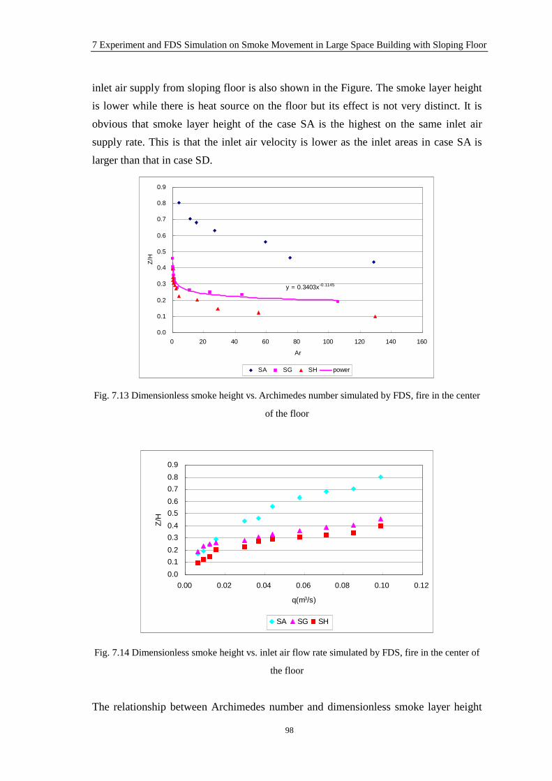
7 Experiment and FDS Simulation on Smoke Movement in Large Space Building with Sloping Floor
98
inlet air supply from sloping floor is also shown in the Figure. The smoke layer height
is lower while there is heat source on the floor but its effect is not very distinct. It is
obvious that smoke layer height of the case SA is the highest on the same inlet air
supply rate. This is that the inlet air velocity is lower as the inlet areas in case SA is
larger than that in case SD.
y = 0.3403x-0.1145
0.0
0.1
0.2
0.3
0.4
0.5
0.6
0.7
0.8
0.9
0 20 40 60 80 100 120 140 160
Ar
Z/H
SA SG SH power
Fig. 7.13 Dimensionless smoke height vs. Archimedes number simulated by FDS, fire in the center
of the floor
0.0
0.1
0.2
0.3
0.4
0.5
0.6
0.7
0.8
0.9
0.00 0.02 0.04 0.06 0.08 0.10 0.12
q(m3/s)
Z/H
SA SG SH
Fig. 7.14 Dimensionless smoke height vs. inlet air flow rate simulated by FDS, fire in the center of
the floor
The relationship between Archimedes number and dimensionless smoke layer height

7 Experiment and FDS Simulation on Smoke Movement in Large Space Building with Sloping Floor
99
for the case SE can be described as equation (7.6).
0.11450.3403z
ArH
−= (7.6)

8 Conclusion
100
8 Conclusion
For the axisymmetric plume, CFD and experiment results agree well with the results
estimated by the NFPA-92B equation and Zukoski equation. The mass entrainment rate
might be overestimated by McCaffrey’s equation. The plume entrainment coefficient of
the wall plume and corner plume are 64% and 48% of the axisymmetric plume
respectively.
The coefficient of the mass flow rate of the balcony plume is between 0.342 and 0.468,
and the balcony plume entrainment coefficient is independent of the fire location.
Compared with the NFPA model, the error range of the results from the experiment and
FDS simulation data in this report is between -0.08 and 0.05. The balcony equation in
NFPA would give good predictions on the mass flow rate.
On the same air supply and smoke exhaust condition, the smoke layer height is lower
while the angle of the sloping floor is larger; the smoke layer height is lower while
there is a heat source on the sloping floor. And the type of ventilation also affects the
smoke layer height.
As the limit of the experiment condition, the further research is needed for the wall and
corner plume.
This report was written as a work report of my stay at the department of civil
engineering of AAU from January 2007 to June 2007. As the time limitation the further
analysis of the result is needed.

Nomenclature
101
Nomenclature
Z--the height of the room, m;
t--time, s;
H--ceiling height above the fire, m;
Q--steady-state heat release rate, kW;
A-- cross-sectional area of the atrium, m2.
Ve--volumetric rate of smoke production, m3/s;
Qc--convective portion o the heat release rate, kW; (Qc=0.7Q)
m--mass flow rate in plume at height Z, kg/s;
ρ--density of smoke, kg/m3;
Tp--adiabatic exhaust temperature, ;
Ta--ambient temperature, ;
m--mass flow of exhaust air, kg/s;
Cp--specific heat of plume gases, kJ/(kg· );
α--growth coefficient;
g--acceleration of gravity, m/s2;
Tf --temperature of heated smoke, K;
T0--temperature of ambient air, K;
∆Tg--gas temperature rise at ceiling, K;
ta--actuation time, s;
τ--time constant, m3/2s3/2;
ρs--density of smoke exhaust ,kg/m3;
Ts--temperature of exhaust smoke, ;
Cm1--the dimensionless entrainment coefficient;
hb--the height of the balcony, m;
Zb--the height above the balcony, m. (Zb=Zp-hb)

References
102
References
[1] J.R. Jones. A Summary of Analytical Method and Case Study Monitoring of Atria.
ASHRAE Transaction. 1993. 1070-1080.
[2] IBryn. Atrium Buildings Environmental Design and Energy Use. ASHRAE
Transaction. 1994. 1082-1091
[3] Chow, W. K. 1989. Smoke movement and design of smoke control in atrium
buildings. International Journal of housing Science and its Application 13(4): 307-322.
[4] Chow, W. K. 1990. Smoke movement and design of smoke control in atrium
building- Part2: Diagrams. International Journal of housing Science and its Application
14(2): 147-159. [5] Ying Ping.1996. Design method for smoke management in atria. Heating,
Ventilating & Air Conditioning 26(5): 55-59.
[6] Morgan H P, Ghosh B K, Garrad G, Pamlitschka R, De Smedt J-C and Schoonbaert
L R. Design methodologies for smoke and heat exhaust ventilation. BRE Report 368,
1999. [7] Chow, W. K. and W. K. Wong. 1993a. on the simulation of atrium fire environment
in Hong Kong using zone models. Journal of Fire Sciences 11(1): 3-51.
[8] Chow, W. K. and W. K. Wong. 1993b. Application of the zone model FIRST on
the development of smoke layer and evaluation of smoke extraction design for atria in
Hong Kong. Journal of Fire Sciences 11(4): 329-349. [9] Chow, W. K. 1989. Smoke movement and design of smoke control in atrium
buildings. International Journal of housing Science and its Application 13(4): 307-322.
[10] Chow, W. K. and C. Y. Chau. 1994. General views on fire aspect of atrium
buildings in Hong Kong. International Journal of housing Science and its Application
18(1): 43-52.
[11] Klote J H and Milke J A. Design of smoke management systems. American Society
of Heating, Refrigerating and Air-conditioning Engineers, Atlanta, GA, 1992.
[12] Klote, J. K. 1997. Prediction of smoke movement in atria: PartⅠ-physical
concepts. ASHRAE Transactions 103(1): 534-544. [13] Klote, J. K. 1997. Prediction of smoke movement in atria: PartⅡ-application to
smoke management. ASHRAE Transactions 103(2): 545-513.
[14] NFPA. 1995. NFPA 92B, Guide for smoke management system in malls, atria and
large area. Quincy, Mass.: National Fire Protection Association.
[15] Brooks, W. N. 1997. Comparison of “regular” and “irregular” methods of
calculating smoke layer interface heights in 1996 BOCA National Building Code.

References
103
ASHRAE Transactions 103(2):554-569.
[16] Xiong Hong. 1994. Modes of smoke exhaust system and performances in atrium
buildings. Heating, Ventilating & Air Conditioning 24(5):25-27.
[17] Ying Ping.1996. Design method for smoke management in atria. Heating,
Ventilating & Air Conditioning 26(5): 55-59. [18] Lougheed, G. K. 1997. Investigation of atrium smoke exhaust effectiveness.
ASHRAE Transactions 103(2): 519-533
[19] Chow, W. K. 1994. A short note on the simulation of atrium smoke filling process
using fire zone models. Journal of Fire Sciences 12(6): 516-528.
[20] Chow, W. K. 1993. Simulation of the atrium fire environment in Hong Kong.
ASHRAE Transactions 99(2): 163-168.
[21] Heskestad G. Engineering relations for fire plumes. Fire Safety Journal, 7,No 1, pp
25-32, 1984.
[22] Zukoski E E. Properties of fire plumes, in Combustion Fundamentals of Fire, Cox
G, Editor. Academic Press, London, 1995.
[23] Michael Poreh, Gordon Garrad. A study of wall and corner plumes. Fire Safety
Journal 34 (2000) 8198
[24] Klote J H and Milke J A. Design of smoke management systems. American Society
of Heating, Refrigerating and Air-conditioning Engineers, Atlanta, GA, 1992.
[25] H.Y. Wang*, M. Coutin, J.M. Most Large-eddy-simulation of buoyancy-driven fire
propagation behind a pyrolysis zone alonga vertical wall. Fire Safety Journal 37 (2002)
259–285
[26] K.B. McGrattan and G.P. Forney, 2004a, Fire Dynamics Simulator—User’s
Manual, National Institute of Standards and Technology, NIST Special Publication
1019, Gaithersburg, MD, 2004.
[27] P. V. Nielsen. Lecture Notes on Scale Model Experiments. Indoor Environmental
Engineering , September,1999
[28] Poreh, M., Morgan, H.P., Marshall, N.R. and Harrison, R. Entrainment by
Two-dimensional Spill Plumes, Fire Safety Journal, 1998, 30:1-19.
[29] Zukoski, E.E., Kubota, T. and Cetegen, B. Entrainment in Fire Plumes, Fire Safety
Journal, 3: 107–121. (1980/81)
[30] McCaffrey, B.J. (1983). Momentum Implication for Buoyant Diffusion Flames,
Combustion and Flame, 52: 149-167.
[31] Cegeten, B., Zukoski, E.E. and Kubota, T. (1984). Entrainment in the near and Far
Field of Plumes, Combustion Science and Technology, 39: 305-331.
References
104
[32] Hinkley, P.L. (1986). Rates of ‘Production’ of Hot Gases in Roof Venting
Experiments, Fire Safety Journal, 10: 57–65.
[33] McCaffrey, B.J. Purely Buoyant Diffusion Flames Some Experimental Results,
NBSIR 79-1910, National Bureau of Standards, October (1979).
[34] McCaffrey, B.J. and Cox, G. Entrainment and Heat Flux of Buoyant Diffusion
Flames, NBSIR 82-2473, National Bureau of Standards, February (1982).
[35] Lee, L. and Emmons, H.W. (1961). A Study of Natural Convection above Line
Fires, J. Fluid Mechanics, 11: 353–368.
[36] Poreh, M., Morgan, H.P., Marshall, N.R. and Harrison, R. (1998). Entrainment by
two dimensional Spill Plumes, Fire Safety Journal, 30:1–19.
[37] Thomas, P.H. (1987). On the Upward Movement of Smoke and Related Shopping
Mall Problems, Fire Safety Journal, 12:191–203.
[38] Law, M. (1995). Measurements of Balcony Smoke Flow, Fire Safety Journal, 24:
189–195.

Appendix A
105
Appendix A
Center fire (Fire A ,300W) Corner fire (Fire C, 300W)
Fig. 1 smoke filling in experiment (300W)
Fire A

Appendix A
106
Fire B
Fire C
Fire D
Fig. 2 Smoke filling by FDS (300W)
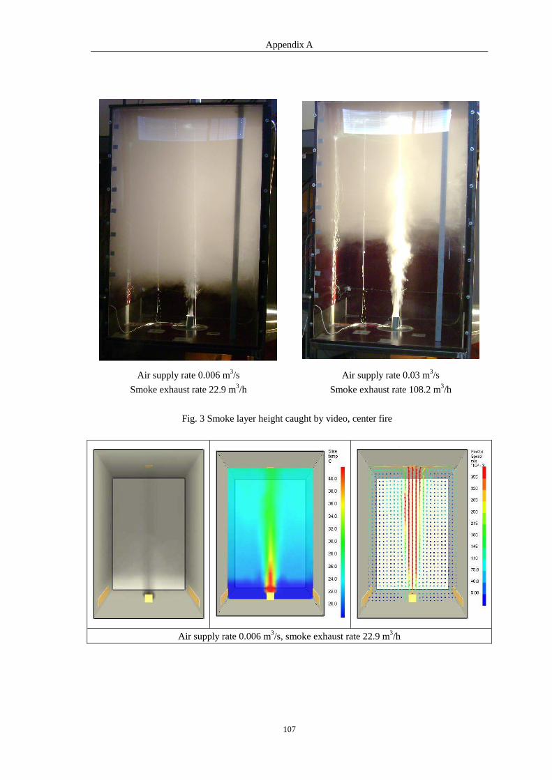
Appendix A
107
Air supply rate 0.006 m3/s
Smoke exhaust rate 22.9 m3/h
Air supply rate 0.03 m3/s
Smoke exhaust rate 108.2 m3/h
Fig. 3 Smoke layer height caught by video, center fire
Air supply rate 0.006 m3/s, smoke exhaust rate 22.9 m3/h

Appendix A
108
Air supply rate 0.03 m3/s, smoke exhaust rate 108.2 m3/h
Fig. 4 Smoke layer height simulated by FDS, center fire
Air supply rate 0.006 m3/s
Smoke exhaust rate 22.9 m3/h
Air supply rate 0.03 m3/s
Smoke exhaust rate 108.2 m3/h
Fig. 5 Smoke layer height caught by video, corner fire
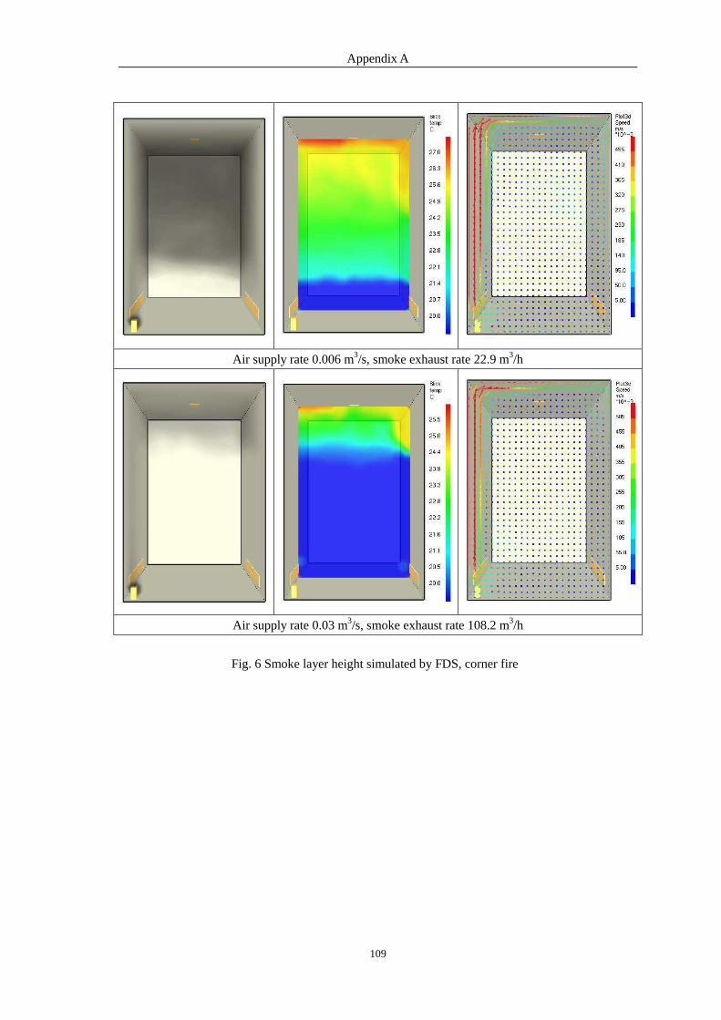
Appendix A
109
Air supply rate 0.006 m3/s, smoke exhaust rate 22.9 m3/h
Air supply rate 0.03 m3/s, smoke exhaust rate 108.2 m3/h
Fig. 6 Smoke layer height simulated by FDS, corner fire
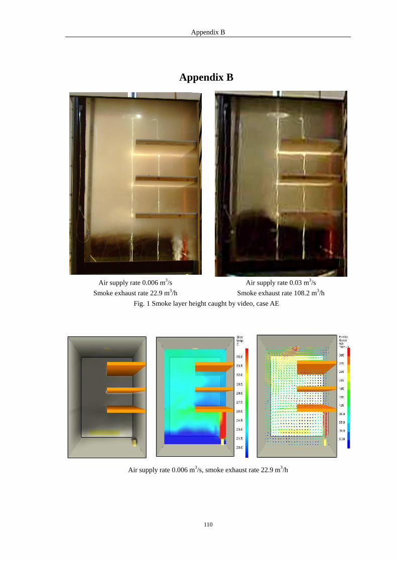
Appendix B
110
Appendix B
Air supply rate 0.006 m3/s
Smoke exhaust rate 22.9 m3/h
Air supply rate 0.03 m3/s
Smoke exhaust rate 108.2 m3/h
Fig. 1 Smoke layer height caught by video, case AE
Air supply rate 0.006 m3/s, smoke exhaust rate 22.9 m3/h
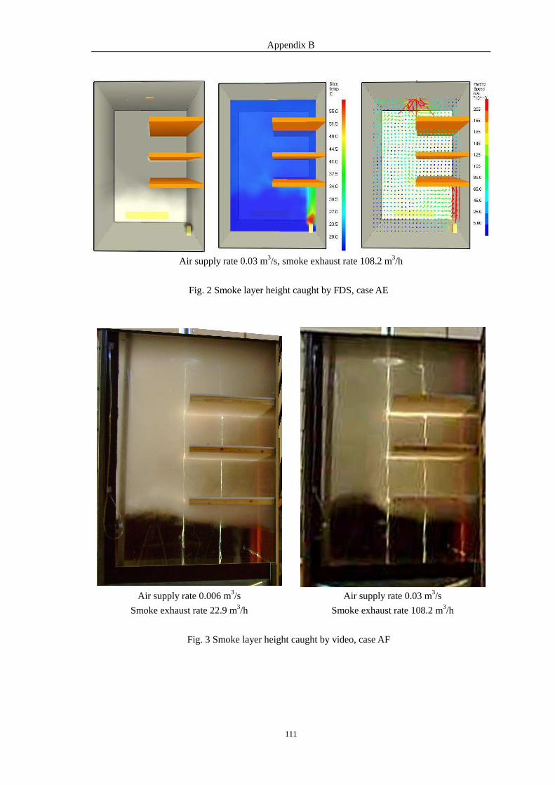
Appendix B
111
Air supply rate 0.03 m3/s, smoke exhaust rate 108.2 m3/h
Fig. 2 Smoke layer height caught by FDS, case AE
Air supply rate 0.006 m3/s
Smoke exhaust rate 22.9 m3/h
Air supply rate 0.03 m3/s
Smoke exhaust rate 108.2 m3/h
Fig. 3 Smoke layer height caught by video, case AF

Appendix B
112
Air supply rate 0.006 m3/s, smoke exhaust rate 22.9 m3/h
Air supply rate 0.03 m3/s, smoke exhaust rate 108.2 m3/h
Fig. 4 Smoke layer height caught by FDS, case AF

Appendix C
113
Appendix C
Air supply rate 0.03 m3/s, smoke exhaust rate
108.5m3/h, 20 degree sloping floor
Air supply rate 0.03 m3/s, smoke exhaust rate
108.5m3/h, 70 degree sloping floor
Fig. 1 smoke layer height caught by video (300W fire in the center)
Air supply rate 0.03 m3/s, smoke exhaust rate 108.5m3/h, 20 degree sloping floor
Fig. 2 smoke layer height caught by video (300W fire in the center, 100W cable on the sloping
floor)

Appendix C
114
Air supply rate 0.03 m3/s
Smoke exhaust rate 108.5 m3/h
Air supply rate 0.03 m3/s
Smoke exhaust rate 108.5 m3/h
100W on the sloping floor
Fig. 3 Fire on the center of 20 degree sloping floor, 300W
Air supply rate 0.03 m3/s, smoke exhaust rate 108.2 m3/h
Fig. 4 smoke layer height caught by FDS, case SA

Appendix C
115
Air supply rate 0.03 m3/s, smoke exhaust rate 108.2 m3/h
Fig. 5 smoke layer height caught by FDS, case SE
Air supply rate 0.03 m3/s, smoke exhaust rate 108.2 m3/h
Fig. 6 smoke layer height caught by FDS, case SG
Air supply rate 0.03 m3/s, smoke exhaust rate 108.2 m3/h
Fig. 7 smoke layer height caught by FDS, case SH


