INVESTIGATION ON PROPERTIES OF CEMENTITIOUS MATERIALS...
118
INVESTIGATION ON PROPERTIES OF CEMENTITIOUS MATERIALS REINFORCED BY GRAPHENE by Zhou Fan B.S. Engineering, Hunan University, 2010 Submitted to the Graduate Faculty of The Swanson School of Engineering in partial fulfillment of the requirements for the degree of Master of Science in Civil Engineering University of Pittsburgh 2014
Transcript of INVESTIGATION ON PROPERTIES OF CEMENTITIOUS MATERIALS...

INVESTIGATION ON PROPERTIES OF CEMENTITIOUS MATERIALS REINFORCED BY GRAPHENE
by
Zhou Fan
B.S. Engineering, Hunan University, 2010
Submitted to the Graduate Faculty of
The Swanson School of Engineering in partial fulfillment
of the requirements for the degree of
Master of Science in Civil Engineering
University of Pittsburgh
2014
ii
UNIVERSITY OF PITTSBURGH
SWANSON SCHOOL OF ENGINEERING
This thesis was presented
by
Zhou Fan
It was defended on
March 26, 2014
and approved by
Jeen-Shang Lin, ScD, Associate Professor, Department of Civil and Environmental Engineering
John Brigham, PhD, Assistant Professor, Department of Civil and Environmental Engineering
Thesis Advisor: Qiang Yu, PhD, Assistant Professor, Department of Civil and Environmental Engineering

iii
Copyright © by Zhou Fan
2014

iv
Graphene nanoplatelet has been found to be able to improve the mechanical and electrical
properties of concrete so that it can make the concrete to be a "smart material". However, its
effects on some other properties of graphene additive concrete, e.g., frost and corrosion
resistance, remain unknown. Therefore, it cannot be directly applied in the construction practice
without further investigation. The purpose of this research is to study the frost resistance and
corrosion resistance of graphene additive mortar as well as the corresponding compressive
strength enhancement induced by the addition of graphene. Here the tests are performed on 5
groups of mortar specimens with the same mix proportion. One group of them were cast by
normal mortar, while each of the other four groups was enriched by an equal amount of C grade
graphene particles (GC), C grade oxidative graphene particles (GOC), M grade graphene
particles (GM) and M grade oxidative graphene particles (GOM), respectively. The dimension of
the C grade graphene nanoplatelets is smaller than that of M grade graphene nanosheets. After 28
days curing, compressive strength test, Young's modulus and Poisson ratio measurement test,
water absorption test, 300 cycles freezing and thawing test and 5-month corrosion test were
performed. The results exhibit that the performance of the GOM group is the best among all of
the experimental groups. The enhancement of the compressive strength of the GOM group is
13.2% compared to the normal mortar. The corrosion and frost resistance of cement are both
slightly improved by adding the M grade oxidative graphene particles. In order to study the
INVESTIGATION ON PROPERTIES OF CEMENTITIOUS MATERIALS
REINFORCED BY GRAPHENE
Zhou Fan, M.S.
University of Pittsburgh, 2014

v
corresponding mechanism from the microstructure of concrete, atomic force microscopy, Raman
spectroscopy and scanning electron microscopy were implemented in this research. The results
of this study indicate that the oxidative graphene nanoplatelets can effectively reduce the
porosity of the cementitious material and therefore increase its strength as well as the corrosion
and the frost resistance.

vi
TABLE OF CONTENTS
ACKNOWLEDGEMENTS .................................................................................................. XVII
1.0 INTRODUCTION ........................................................................................................ 1
1.1 GENERAL............................................................................................................ 1
1.2 THESIS OUTLINE ............................................................................................. 3
2.0 LITERATURE REVIEW ............................................................................................ 4
2.1 CEMENT ENHANCED BY C-NANOTUBES ................................................. 4
2.2 CEMENT ENHANCED BY GRAPHENE ........................................................ 5
2.3 CARBON NANO-COMPOSITE OXIDATION ............................................... 8
2.4 FREEZING & THAWING TESTS ................................................................... 9
2.5 CORROSION TESTS ....................................................................................... 11
2.6 ATOMIC FORCE MICROSCOPY ................................................................. 12
2.7 RAMAN SPECTROSCOPY ............................................................................. 13
3.0 EXPERIMENTAL PROGRAM ............................................................................... 17
3.1 EXPERIMENT DESIGN .................................................................................. 17
3.2 SPECIMEN PREPARATION .......................................................................... 18
3.2.1 Graphene oxidation ........................................................................................ 18
3.2.2 Materials and casting procedure ................................................................... 19
3.3 TESTING............................................................................................................ 23

vii
3.3.1 Trial tests ......................................................................................................... 23
3.3.1.1 Compressive strength trial ................................................................. 23
3.3.1.2 Water absorption trial test ................................................................. 24
3.3.2 Compressive strength test and Young's modulus & Poisson's ratio measurement ................................................................................................... 25
3.3.2.1 Introduction ......................................................................................... 25
3.3.2.2 Apparatus ............................................................................................. 26
3.3.2.3 Test setup and procedure ................................................................... 26
3.3.3 Water absorption test ..................................................................................... 28
3.3.3.1 Introduction ......................................................................................... 28
3.3.3.2 Apparatus ............................................................................................. 28
3.3.3.3 Test setup and procedure ................................................................... 29
3.3.4 Freezing and thawing test .............................................................................. 29
3.3.4.1 Introduction ......................................................................................... 29
3.3.4.2 Apparatus ............................................................................................. 29
3.3.4.3 Test setup and procedure ................................................................... 30
3.3.5 Corrosion test .................................................................................................. 34
3.3.5.1 Introduction ......................................................................................... 34
3.3.5.2 Apparatus ............................................................................................. 34
3.3.5.3 Test setup and procedure ................................................................... 35
4.0 EXPERIMENTAL RESULTS AND DISCUSSION ............................................... 37
4.1 COMPRESSIVE STRENGTH TEST AND YOUNG'S MODULUS & POISSON'S RATIO MEASUREMENT ............................................................ 37
4.1.1 Results .............................................................................................................. 37

viii
4.1.2 Discussion ........................................................................................................ 40
4.2 WATER ABSORPTION TEST........................................................................ 41
4.2.1 Results .............................................................................................................. 41
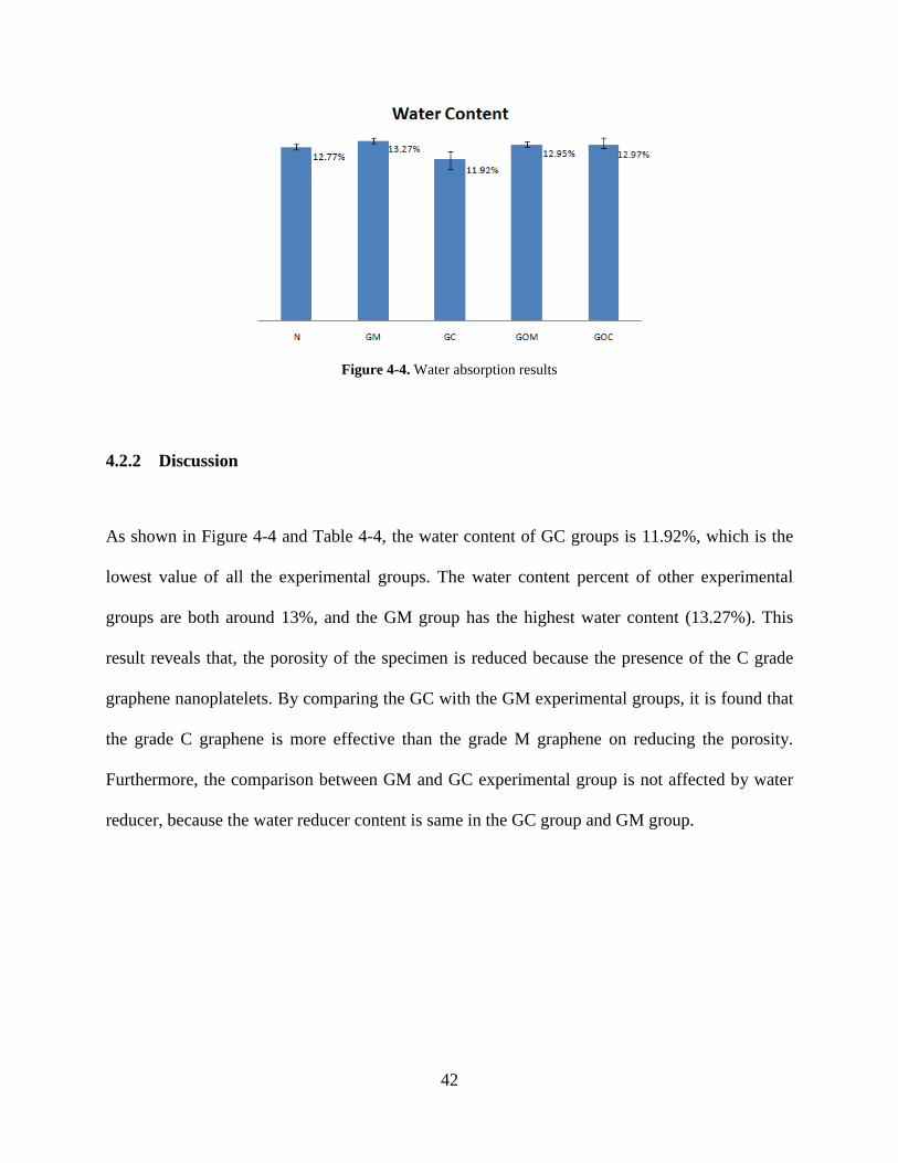
4.2.2 Discussion ........................................................................................................ 42
4.3 FREEZING AND THAWING TEST .............................................................. 43
4.3.1 Results .............................................................................................................. 43
4.3.2 Discussion ........................................................................................................ 45
4.4 CORROSION TEST ......................................................................................... 47
4.4.1 Results .............................................................................................................. 47
4.4.2 Discussion ........................................................................................................ 48
5.0 MICROSCOPIC PROBE .......................................................................................... 51
5.1 SPECIMEN PREPARATION .......................................................................... 51
5.1.1 Specimen casting ............................................................................................. 51
5.1.2 Specimen polishing ......................................................................................... 52
5.2 ATOMIC FORCE MICROSCOPE OBSERVATION .................................. 53
5.2.1 Test instrumentation and setup ..................................................................... 53
5.2.2 Results and discussion .................................................................................... 54
5.3 RAMAN SPECTROSCOPY TEST ................................................................. 57
5.3.1 Test instrumentation ...................................................................................... 57
5.3.2 Results and discussion .................................................................................... 57
5.4 SCANNING ELECTRON MICROSCOPE OBSERVATION ..................... 60
5.4.1 Test instrumentation ...................................................................................... 60
5.4.2 Results and discussion .................................................................................... 60

ix
6.0 SUMMARY, CONCLUSIONS, AND RECOMMENDATIONS .......................... 62
6.1 SUMMARY ........................................................................................................ 62
6.2 CONCLUSIONS ................................................................................................ 63
6.3 RECOMMENDATIONS .................................................................................. 64
APPENDIX A .............................................................................................................................. 66
APPENDIX B .............................................................................................................................. 91
BIBLIOGRAPHY ....................................................................................................................... 96

x
LIST OF TABLES
Table 3-1. Mix design for tests ..................................................................................................... 20
Table 3-2. Oxidative graphene content ......................................................................................... 21
Table 3-3. Specimen composition................................................................................................. 21
Table 3-4. Specimen casting information ..................................................................................... 23
Table 3-5. Compressive strength trial test results ......................................................................... 24
Table 3-6. Water absorption strength trial test results .................................................................. 25
Table 4-1. Compressive strength results ....................................................................................... 38
Table 4-2. Young's modulus results .............................................................................................. 38
Table 4-3. Poisson's ratio results ................................................................................................... 39
Table 4-4. Water absorption results .............................................................................................. 41
Table 4-5. The average compressive strength test records of the N group ................................... 47
Table A-1. Test results of water absorption trial test: N ............................................................... 66
Table A-2. Test results of water absorption trial test: 0.1% GC ................................................... 66
Table A-3. Test results of water absorption trial test: 0.1% GM .................................................. 66
Table A-4. Test results of water absorption trial test: 0.1% GOC ................................................ 67
Table A-5. Test results of water absorption trial test: 0.1% GOM ............................................... 67
Table A-6. Test results of water absorption trial test: 0.2% GC ................................................... 67
Table A-7. Test results of water absorption trial test: 0.2% GM .................................................. 67
Table A-8. Test results of water absorption trial test: 0.4% GC ................................................... 68

xi
Table A-9. Test results of water absorption trial test: 0.4% GM .................................................. 68
Table A-10. Titration records before the first compression test ................................................... 68
Table A-11. Titration records before the second compression test .............................................. 69
Table A-12. Titration records before the last compression test .................................................... 69
Table A-13. Compressive strength records and calculations of the N group ............................... 70
Table A-14. Young's modulus records and calculations of the N group ...................................... 70
Table A-15. Poisson's ratio records and calculations of the N group ........................................... 70
Table A-16. Compressive strength records and calculations of the GM group ............................ 71
Table A-17. Young's modulus records and calculations of the GM group ................................... 71
Table A-18. Poisson's ratio records and calculations of the GM group ....................................... 71
Table A-19. Compressive strength records and calculations of the GC group ............................. 72
Table A-20. Young's modulus records and calculations of the GC group ................................... 72
Table A-21. Poisson's ratio records and calculations of the GC group ........................................ 72
Table A-22. Compressive strength records and calculations of the GOM group ......................... 73
Table A-23. Young's modulus records and calculations of the GOM group ................................ 73
Table A-24. Poisson's ratio records and calculations of the GOM group ..................................... 73
Table A-25. Compressive strength records and calculations of the GOC group .......................... 74
Table A-26. Young's modulus records and calculations of the GOC group ................................. 74
Table A-27. Poisson's ratio records and calculations of the GOC group ..................................... 74
Table A-28. The weight records of the N group ........................................................................... 77
Table A-29. The weight records of the GM group ....................................................................... 78
Table A-30. The weight records of the GC group ........................................................................ 79
Table A-31. The weight records of the GOM group .................................................................... 80

xii
Table A-32. The weight records of the GOC group ..................................................................... 81
Table A-33. The length records of the N group ............................................................................ 82
Table A-34. The length records of the GM group ........................................................................ 83
Table A-35. The length records of the GC group ......................................................................... 84
Table A-36. The length records of the GOM group ..................................................................... 85
Table A-37. The length records of the GOC group ...................................................................... 86
Table A-38. The average weight change percentage of each groups ........................................... 87
Table A-39. The average length change percentage of each groups ............................................ 88
Table A-40. The corrosion test records of the N group ................................................................ 88
Table A-41. The corrosion test records of the GM group ............................................................. 89
Table A-42. The corrosion test records of the N group ................................................................ 89
Table A-43. The corrosion test records of the N group ................................................................ 90
Table A-44. The corrosion test records of the N group ................................................................ 90
Table B-45. Characteristics of xGnP® grade M graphene nanoplatelets (XG Sciences, 2013)... 92
Table B-46. Sand sieve data.......................................................................................................... 95

xiii
LIST OF FIGURES
Figure 2-1. Schematic diagram of regulation mechanism of GO on cement hydration crystals (Lv et al. 2013) ................................................................................................................... 6
Figure 2-2. Schematic diagram of reaction between graphene and cement (Sedaghat et al. 2013) 7
Figure 2-3. Process of oxidation (Alkhateb et al. 2012) ................................................................. 8
Figure 2-4. Freezing and thawing machine (Hamoush et al. 2012) .............................................. 10
Figure 2-5. Hydrated Portland cement with pristine graphene nanoplatelets (Alkhateb et al. 2013) ................................................................................................................................... 12
Figure 2-6. AFM images of the smallest lamellae of GO (Lv et al. 2013) ................................... 12
Figure 2-7. Raman spectra of dark particles of original concrete (Pešková et al. 2011) .............. 13
Figure 2-8. Comparison of Raman spectra between graphite and graphene (Ferrari et al. 2006) 14
Figure 2-9. SEM image of cement mixed with pristine graphene (Alkhateb et al. 2006) ............ 15
Figure 2-10. (A) no GO; (B) GO 0.01%; (C) 0.02%; (D) 0.03%; (E) 0.04%; and (F) 0.05% (Lv et al. 2013) ..................................................................................................................... 15
Figure 3-1. Graphene oxidation set-up ......................................................................................... 18
Figure 3-2. Casting procedure (a) cement and sand; (b) graphene with water; (c) mixer; and (d) specimen vibration .................................................................................................... 22
Figure 3-3. Specimens (1 batch): (a) fresh cast specimens and (b) 28-day cured specimens ....... 22
Figure 3-4. Apparatus for compressive strength test and Young's Modulus & Poisson's Ratio measurement: (a) Concrete Elastic Modulus Meter, (b) TEST MARK CM4000 compression machine ................................................................................................ 26
Figure 3-5. Apparatus for freezing and thawing test: (a) water container and (b) chest freezer .. 30

xiv
Figure 3-6. Stainless steel rods embedded in the end ................................................................... 30
Figure 3-7. Specimen configuration ............................................................................................. 31
Figure 3-8. Freezing phase setup .................................................................................................. 32
Figure 3-9. Thawing phase setup .................................................................................................. 33
Figure 3-10. Agents for corrosion test: (a) 15% ammonium nitrate solution; (b) ammonium nitrate; (c) burette; and (d) sodium hydroxide solution, phenolphthalein and formaldehyde (from left to right) .............................................................................. 35
Figure 4-1. Compressive strength results...................................................................................... 38
Figure 4-2. Young's modulus results ............................................................................................ 39
Figure 4-3. Poisson's ratio results ................................................................................................. 39
Figure 4-4. Water absorption results ............................................................................................. 42
Figure 4-5. Weight change percentage of all the specimens ........................................................ 43
Figure 4-6. Average weight change percentage all the groups ..................................................... 44
Figure 4-7. Length change percentage of all the specimens ......................................................... 44
Figure 4-8. Average length change percentage of all the groups ................................................. 45
Figure 4-9. Average relative length of all the groups ................................................................... 48
Figure 4-10. Specimens tested by phenolphthalein: (a) corrosion for 1 month; (b) 3 months; and (c) 5 months ............................................................................................................... 49
Figure 5-1. Microscope observation samples ............................................................................... 52
Figure 5-2. Polishing paste and disks ........................................................................................... 52
Figure 5-3. Atomic force microscope (PINSE, 2014) .................................................................. 53
Figure 5-4. The N sample's image obtained by AFM ................................................................... 54
Figure 5-5. The GM sample's image obtained by AFM ............................................................... 54
Figure 5-6. The GC sample's image obtained by AFM ................................................................ 55
Figure 5-7. The GOM sample's image obtained by AFM ............................................................ 55

xv
Figure 5-8. The GOC sample's image obtained by AFM ............................................................. 56
Figure 5-9. Renishaw inVia Raman microscope (PINSE, 2014).................................................. 57
Figure 5-10. Raman spectroscopy observation results of GM ...................................................... 58
Figure 5-11. Raman spectroscopy results of GC cement sample ................................................. 58
Figure 5-12. Optical microscope image of GC cement sample .................................................... 58
Figure 5-13. AFM images of GC simple after Raman spectroscopy location .............................. 59
Figure 5-14. JEOL JSM-6510LV/LGS scanning electron microscope (PINSE, 2014) ............... 60
Figure 5-15. SEM images of GC sample ...................................................................................... 61
Figure 5-16. SEM images of GC sample ...................................................................................... 61
Figure A-1. Compressive force vs. longitudinal displacement of the N group ............................ 75
Figure A-2. Compressive force vs. longitudinal displacement of the GM group ......................... 75
Figure A-3. Compressive force vs. longitudinal displacement of the GC group .......................... 76
Figure A-4. Compressive force vs. longitudinal displacement of the GOM group ...................... 76
Figure A-5. Compressive force vs. longitudinal displacement of the GOC group ....................... 77
Figure A-6. The weight records of the N group............................................................................ 78
Figure A-7. The weight records of the GM group ........................................................................ 79
Figure A-8. The weight records of the GC group ......................................................................... 80
Figure A-9. The weight records of the GOM group ..................................................................... 81
Figure A-10. The weight records of the GOC group .................................................................... 82
Figure A-11. The length records of the N group .......................................................................... 83
Figure A-12. The length records of the GM group ....................................................................... 84
Figure A-13. The length records of the GC group ........................................................................ 85
Figure A-14. The length records of the GOM group .................................................................... 86

xvi
Figure A-15. The length records of the GOC group ..................................................................... 87
Figure B-16. Raman spectroscopy of xGnP® grade M graphene nanoplatelets (XG Sciences, 2013) .......................................................................................................................... 91
Figure B-17. XRD patterns of xGnP® grade C graphene nanoplatelets (XG Sciences, 2013) .... 92
Figure B-18. Raman spectroscopy of xGnP® grade C graphene nanoplatelets (XG Sciences, 2013) .......................................................................................................................... 93
Figure B-19. XPS analysis of xGnP® grade C graphene nanoplatelets (XG Sciences, 2013) ..... 93
Figure B-20. Raman spectroscopy of water on glass slide obtained by Renishaw inVia ............. 94
Figure B-21. Raman spectroscopy of water with GM obtained by Renishaw inVia .................... 94

xvii
ACKNOWLEDGEMENTS
First, I would like to thank my advisor Dr. Yu for providing me the opportunity to do the
research and supporting me throughout my graduate studies. I could not finish this thesis without
his instruction and education.
I would also like to acknowledge my committee members, Dr. John Brigham and Dr.
Jeen-Shang Lin. Thank you for your precious time and instructive advice.
Many thanks to the Post Doctorial Associate of our group, Dr. Qiong Liu. Thank you for
helping me design the experiments, guiding me to perform the tests and giving me suggestions.
I would like to extend my gratitude and appreciation to Dr. Susheng Tan and Tong Teng,
the PhD student of Dr. Yu, for helping me with the microscopic experiments.
Furthermore, I want to acknowledge Dr. Julie M. Vandenbossche and her graduate
students Nicole Dufalla, Zichang Li and Feng Mu. Thank you for providing me the experimental
apparatus and equipment to make my experiments possible.
Finally, I would like to take this opportunity to express my thanks to my parents and my
wife Wenjie Huang for their continuous support throughout my graduate studies.

1
1.0 INTRODUCTION
1.1 GENERAL
Concrete, with its low price, simple production process, high compressive strength and excellent
durability, is one of major civil engineering materials and has been deeply studied and widely
used. However, with the applications of new technologies, demands are more and more intense
on the innovative concrete, which is stronger and smarter. It means that people want concrete to
be able to provide strength for structure, as well as to integrate other functional applications,
such as self-monitoring. Thus, carbon fiber additive concrete comes forth.
Adding carbon fibers can improve the electric conductivity of concrete for various
applications such as electromagnetic interference shielding, lateral guidance in automatic
highways, traffic monitoring, weighing in motion, deicing and self-monitoring (Hou et al. 2006).
With the development of nano materials, carbon nano-fibers were gradually being studied, such
as carbon nanotubes and graphene nanoplatelets. During recent decades, using carbon nanotubes
to improve the performance of concrete has been attracting increasing interests. However, the
research about graphene additive concrete is still in its infancy.
Graphene is a two-dimensional carbon molecule in which the structure is quite similar to
graphite. "Graphene" refers to a single layer of graphite, and in some cases means a few layers of
graphite as well. Because of its unique structure, the surface area of graphene nanoplatelets is

2
greatly increased to make itself an ideal nano material which can be used to reduce the electric
resistivity of concrete.
Furthermore, it has been noted that enriched by graphene nano-material merely 0.01 % to
1 % of the weight of the Portland cement, the concrete compressive strength could be improved
from 5% to 40%, depending on the particle dimension of the additive materials and the different
treatment methods that have been used in the experiments. Thus, this technology could have a
wide application in civil engineering.
However, except the current studies on the compressive strength, tensile strength and the
flexural strength of this new type of "cement", some other important material properties of this
"smart material" still need to be investigated, e.g., the frost and corrosion resistance.
In practice, the concrete structure is subject to alternating hot and cold external
environment during each calendar year, especially in high latitude regions. The annual
temperature difference in some areas can reach 100 °C. Under such extreme conditions, frost
resistance of concrete is particularly important. Similarly, the structures are expected to be
contacted by water, such as ground water, acid rain and sea water, and therefore under attack by
the corrosive chemicals in the water. If the application of a new additive resulted in weakening
of concrete frost or corrosion resistance, then the engineering application of this new material is
significantly limited. Thus it is of great importance to study the frost and corrosion resistance of
graphene additive concrete.
Therefore, the main purpose of this research is to study the frost resistance and corrosion
resistance of cementitious materials which are reinforced by graphene nanoplatelets, with an aim
of promoting the pace of using this technique in practice and filling the gaps of the studies in this
area. In addition, this study will try to explore the mechanism of how mechanical properties of

3
Portland cement can be enhanced by graphene, which has not yet been fully explained. In detail,
this study sets up a series of tests on graphene additive Portland cement to study its concrete
compressive strength, Young's model, Poisson's ratio, frost resistance and corrosion resistance.
The processes, results and related discussions of these tests will be introduced in following
chapters.
1.2 THESIS OUTLINE
The outline of the thesis is organized as follows.
Chapter 2 presents a literature review of the current studies about graphene additive
cementitious materials.
Chapter 3 describes the experimental program of this research.
Chapter 4 reports the experimental results and presents the discussions based on the
experiments.
Chapter 5 shows the microscope observation results.
Chapter 6 presents the conclusions, summaries and recommendations of this research.
4
2.0 LITERATURE REVIEW
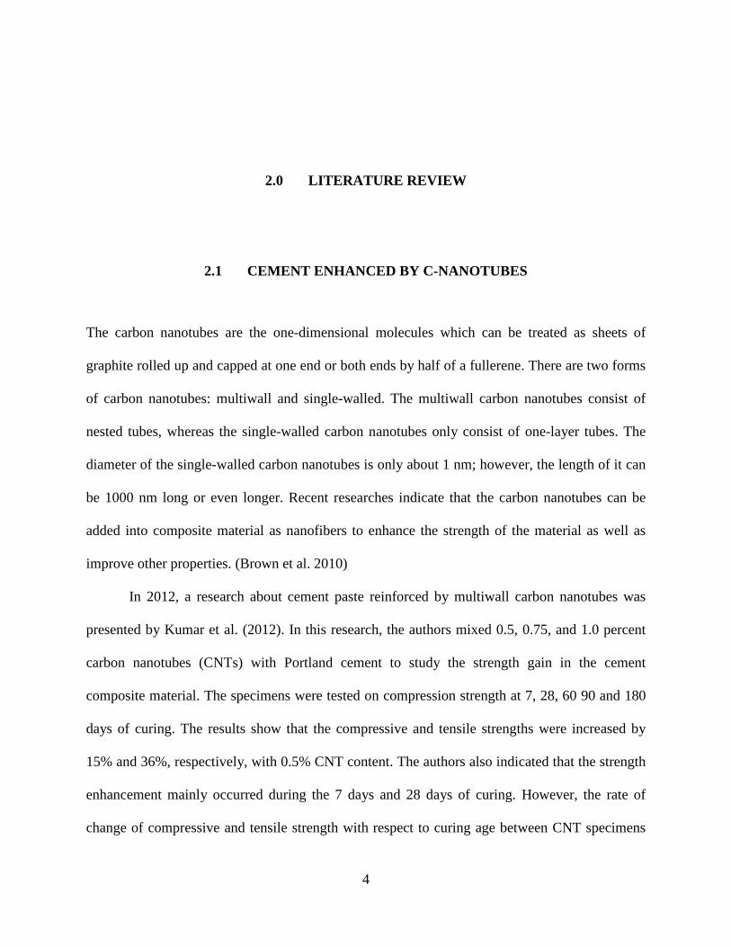
2.1 CEMENT ENHANCED BY C-NANOTUBES
The carbon nanotubes are the one-dimensional molecules which can be treated as sheets of
graphite rolled up and capped at one end or both ends by half of a fullerene. There are two forms
of carbon nanotubes: multiwall and single-walled. The multiwall carbon nanotubes consist of
nested tubes, whereas the single-walled carbon nanotubes only consist of one-layer tubes. The
diameter of the single-walled carbon nanotubes is only about 1 nm; however, the length of it can
be 1000 nm long or even longer. Recent researches indicate that the carbon nanotubes can be
added into composite material as nanofibers to enhance the strength of the material as well as
improve other properties. (Brown et al. 2010)
In 2012, a research about cement paste reinforced by multiwall carbon nanotubes was
presented by Kumar et al. (2012). In this research, the authors mixed 0.5, 0.75, and 1.0 percent
carbon nanotubes (CNTs) with Portland cement to study the strength gain in the cement
composite material. The specimens were tested on compression strength at 7, 28, 60 90 and 180
days of curing. The results show that the compressive and tensile strengths were increased by
15% and 36%, respectively, with 0.5% CNT content. The authors also indicated that the strength
enhancement mainly occurred during the 7 days and 28 days of curing. However, the rate of
change of compressive and tensile strength with respect to curing age between CNT specimens

5
and control specimens was seen to be very similar. Thus, the authors claimed that the strength
enhancement is primarily because of cement hydration, rather than the reaction between CNTs
and cement compounds.
In the same year, Abu Al-Rub et al. (2012) presented research about the effect of
functionalized CNTs and carbon nanofibers (CNFs) on the mechanical properties of cement
composites. The concentrations of treated and untreated CNFs and CNTs were 0.1% and 0.2%
by weight of cement. The treated CNFs and CNTs were oxidized in a solution of sulfuric acid
and nitric acid and washed clean before being added into the cement paste. The results showed
that, compare to the plain cement, the average enhancements on ductility, flexural strength,
Young's modulus and toughness modulus were 73%, 60%, 25% and 170%, respectively. The
authors also suggested that the reasonable value of the concentration of graphene by weight is
around 0.1%.
Besides, Konsta-Gdoutos et al. (2010) presented research to study the effects of
ultrasonic energy and surfactant concentration on the dispersion of multiwall CNTs for cement
based material reinforcement. The authors concluded that, for proper dispersion, the application
of ultrasonic energy is necessary and the ratio of surfactant to CNTs is suggested to be 4.0.
2.2 CEMENT ENHANCED BY GRAPHENE
In 2013, Alkhateb et al. (2013) showed a series methods to investigate the properties of
cementitious material reinforced by graphene nanoplatelets. In this research, the authors
presented a general framework for using a systematic approach to study the cementitious
materials. These research approaches include molecular dynamics simulations (MD) as well as

6
observation via atomic force microscopy (AFM), scanning electron microscopy (SEM), X-Ray
diffraction (XRD) and resonant ultrasound spectroscopy.
Figure 2-1. Schematic diagram of regulation mechanism of GO on cement hydration crystals (Lv et al. 2013)
Lv et al. (2013) presented research about the effect of graphene oxide nanosheets (GO) in
cement composites. The graphene nanoplatelet used in this research is relatively small (<30 μm).
The functionalized graphene is treated by 98% H2SO4 and NaNO3. The experimental results
showed that, when the content of GO was 0.03%, the cement composites exhibited striking
increase in tensile strength (78.6%), flexural strength (60.7%) and compressive strength (38.9%),
7
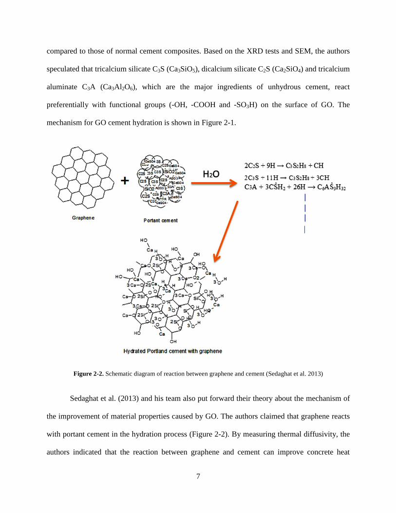
compared to those of normal cement composites. Based on the XRD tests and SEM, the authors
speculated that tricalcium silicate C3S (Ca3SiO5), dicalcium silicate C2S (Ca2SiO4) and tricalcium
aluminate C3A (Ca3Al2O6), which are the major ingredients of unhydrous cement, react
preferentially with functional groups (-OH, -COOH and -SO3H) on the surface of GO. The
mechanism for GO cement hydration is shown in Figure 2-1.
Figure 2-2. Schematic diagram of reaction between graphene and cement (Sedaghat et al. 2013)
Sedaghat et al. (2013) and his team also put forward their theory about the mechanism of
the improvement of material properties caused by GO. The authors claimed that graphene reacts
with portant cement in the hydration process (Figure 2-2). By measuring thermal diffusivity, the
authors indicated that the reaction between graphene and cement can improve concrete heat

8
dissipation during the hydration process. This led to thermal cracking decrease in specimens so
that graphene could improve the strength of the cementitious materials.
2.3 CARBON NANO-COMPOSITE OXIDATION
The oxidation process can add functional groups on the surface of the carbon molecules in order
to change its properties of interaction with cement. Thus, the oxidation is also called
functionalization. Current literature suggests that the oxidation process is achieved by using high
concentration acid to react with graphene particles. In some cases, catalysts are needed.
In Abu Al-Rub's research (Abu Al-Rub et al. 2012), the oxidation procedure was
performed as follow: 0.9 g CNTs and CNFs was added into 300ml acid solution. The sulfuric to
nitric acid ratio of this solution is 2:1. All the substrate was refluxed for 1 h at 85 °C and
continuously stirred with a magnetic stirrer. The solution was diluted in 4 L distilled water and
then filtered through a polytetrafluorethylene membrane.
Figure 2-3. Process of oxidation (Alkhateb et al. 2012)

9
As shown in Figure 2-3, the oxidation method used by Alkhateb et al. (2013) is similar
with the method proposed by Rosca et al. (2005). 3 g of graphene and 300 ml of nitric acid were
mixed in a 500-mL glass flask and dispersed in the ultrasound disperser for 15 min. The total
reacting time is 24 hours and then the mixture is purified by filtration using distilled water.
Another oxidation method presented by Lv et al. (2013) is relatively complicated than the
2 methods mentioned previously. As described by the authors, 5g graphite, 30g 98% H2SO4 and
2 g NaNO3 was added into a three-necked round-bottomed flask placed in an ice bath (<5 °C)
under stirring. 6g KMnO4 was gently added to the flask. The flask was maintained at 5 °C for 1
hour until the color of the solution had turned green. Then it was heated and kept to 35 °C for 12
hours. Then 100 mL deionized water was slowly added in and was heated to 90 °C. Then 300
mL deionized water and 30g hydrogen peroxide were slowly added in. After the color of the
solution changed from brown to bright yellow, the mixture was filtered to neutral pH.
2.4 FREEZING & THAWING TESTS
The slow freezing method and the fast freezing method are two main concrete frost resistance
test methods. Existing international standards include ASTM C666-97 and ASTM C672-2003
(United States), BS 5075 (British), CSA A23.2-94 (Canada), NS 3473-92 and NS 4320-86
(Norway) and TC117-2FDC (Sweden) etc. In slow-freezing method, loss of compressive
strength is generally used as a criterion. However, according to the fact that concrete damage in
freezing tests is caused by the internal tension cracking, the specimens are sensitive to
distribution of the tension cracks. It means the results of the compressive strength test are
unpredictable because of the randomness of the internal tension cracks. Thus, the results of slow-

10
freezing method are unrepeatable for the other researchers. Furthermore, due to the long test
cycle, heavy workload, the experimental error and other shortcomings, the slow-freezing method
is seldom used now and the fast-freezing method wins the popularity. In addition to the
compressive strength loss, the mass loss ratio is now used as a criterion in the fast-freezing as
well as the slow-freezing methods. It is worth mention here that there is a certain error of this
evaluation criterion, and therefore, in most cases, it is used in conjunction with the relative
dynamic modulus loss to evaluate the frost resistance. (Zhang et al. 2008)
Figure 2-4. Freezing and thawing machine (Hamoush et al. 2012)
At present, there is no research using freezing and thawing test to evaluate the properties
of the cementitious material reinforced by graphene nanoplatelets. In order to fully understand
the freezing and thawing test, some researches about freezing and thawing tests were reviewed.
Shang and Yi (2013) presented a research about the durability of air-entrained concrete by
freezing and thawing test. Their freezing and thawing cycles consisted of alternately lowering the
temperature of the specimens from 6 °C to -15 °C and raising it from -15 °C to 6 °C. The

11
specimen size was 100 mm × 100 mm× 400 mm. The dynamic modulus of elasticity and weight
loss of the specimens were measured before the freezing cycles. Hamoush et al. (2011) also used
freezing and thawing test to evaluate the durability of high strength concrete. The freezing and
thawing cycles were performed using the specialized machine which is shown in Figure 2-4.
Their experiments were performed according to ASTM C-666 procedure-A. The dynamic
modulus of elasticity, dynamic modulus of rigidity, Poisson's ratio, flexural strength and
durability factors were investigated after each number of cycles.
2.5 CORROSION TESTS
Schneider and Chen (1997) presented research about the chemomechanical effect and the
mechanochemical effect on high-performance concrete. In this research, the specimens were
subjected to flexural loads with a level of 30% of their initial strengths, while immersed into a
5% ammonium sulfate solution, a 10% ammonium nitrate solution, or a saturated calcium
hydroxide solution.
In 2004, Schneider and Chen presented another experiment used ammonium nitrate
solution to corrode high-performance concrete. The concentrations of ammonium nitrate in the
solution are 10%, 5%, 1% and 0.1%. The authors also mentioned that during the test the
solutions were replaced as needed to maintain the solution concentration.

12
2.6 ATOMIC FORCE MICROSCOPY
AFM is a perfect technique to study nanomaterials because it can provide high resolution
topography of microstructure, combine advantages of digital three-dimensional morphological
information in atmosphere, and have no vacuum requirement. (Yang et al. 2003)
Figure 2-5. Hydrated Portland cement with pristine graphene nanoplatelets (Alkhateb et al. 2013)
Alkhateb et al. (2013) indicated that AFM can be used for graphene nanoplatelet cement
observation. In the paper, the authors exhibited some images of AFM obtained by them, e.g.,
Figure 2-5. The authors claimed that, in Figure 2-5a, a graphene platelet at the top-right corner is
identified, and the 3D phase image in Figure 2-5b confirms the graphene platelet is clearly
correlated with the hi-stiffness phase topography.
Figure 2-6. AFM images of the smallest lamellae of GO (Lv et al. 2013)

13
Lv et al. (2013) also indicated that the AFM technique can be used to probe the products
of graphene oxidation and help to examine the obtaining of GO nanosheets suspension solution.
As shown in figures, the images indicated that single irregular lamella of GO is observed with a
size of 80 ~ 260 nm (Figure 2-6 a), and a thickness less than 8 nm (Figure 2-6 b).
2.7 RAMAN SPECTROSCOPY
In 1928, Sir C.V. Raman was awarded the Nobel Prize for discovering an effect which relies on
the fact that when light interacts with matter, the incoming wavelength shifted as vibrational
transitions are excited. This effect then is known as the Raman Effect (Zoubir, 2012). In the last
eighty years, the Raman Effect has been maturely developed to be applied in practice. Nowadays,
the Raman spectroscopy is an ideal tool to identify the molecules of interested materials.
Figure 2-7. Raman spectra of dark particles of original concrete (Pešková et al. 2011)

14
Pešková et al. (2011) presented research to study fired concrete by using Raman
spectroscopy. The specimens were placed in furnace at 1200 °C for 160 minutes. The mixture of
dicalcium silicate and gehlenite was found on the surface of heated concrete. Figure 2-7 showed
the Raman spectra of dark particles of original concrete.
Figure 2-8. Comparison of Raman spectra between graphite and graphene (Ferrari et al. 2006)
Ferrari et al. (2006) used Raman spectroscope to study graphene and graphite. The
Raman spectrum is shown in Figure 2-8. The authors concluded that graphene's electronic
structure was uniquely captured in its Raman spectrum so that an unambiguous, high-throughput
and nondestructive identification of graphene was provided via the Raman spectroscopy
technique.
Scanning electron microscopy is another powerful "weapon" to study the microstructure of
cementitious materials. The scanning electron microscope is particularly suitable for samples
with rough surface because of its far depth of field, high resolution and strong magnification

15
ability. Furthermore, comparing to AFM, scanning electron microscopy does not need to
physically contact the specimen. In general, SEM has wider application than AFM in the
researches on cementitious materials.
Figure 2-9. SEM image of cement mixed with pristine graphene (Alkhateb et al. 2006)
Alkhateb et al. (2013) used SEM in their research to observe graphene in the cement. As
shown in Figure 2-9, SEM has identified a graphene platelet in the exfoliated pristine graphene-
cement specimens.
Figure 2-10. (A) no GO; (B) GO 0.01%; (C) 0.02%; (D) 0.03%; (E) 0.04%; and (F) 0.05% (Lv et al. 2013)

16
Lv et al. (2013) also performed the SEM observation in their study. Figure 2-10 shows
the C-S-H crystal flower growing status of different specimens which were cast with different
graphene concentration.

17
3.0 EXPERIMENTAL PROGRAM
In this chapter the details of the experimental program including experiment design, specimen
preparation, and experiment procedure, are reported.
3.1 EXPERIMENT DESIGN
A series of tests were performed in order to study the effects of normal graphene and oxidized
graphene on the cementitious material as well as the influence of different particle size on the
material. They included compression strength test, the Young's modulus and the Poisson's ratio
measurement, corrosion test and freezing & thawing test. For each type of test, the specimens
were divided into four experimental groups and one control group. In the four experimental
groups, the specimens were cast with the additive of C grade graphene particles (GC), C grade
oxidative graphene particles (GOC), M grade graphene particles (GM) and M grade oxidative
graphene particles (GOM), respectively. The specimens in the control group were cast by normal
mortar (N). The details of the graphene powder used will be given in the following section.
Because of the limitations of test conditions, equipment and materials, all of the graphene
specimens of the experimental groups were cast with the same graphene concentration which is
determined in the trail test. Thus, factor of graphene concentration is not concerned in the
experimental program.

18
3.2 SPECIMEN PREPARATION
3.2.1 Graphene oxidation
In the Graphene oxidation, predetermined quantities of raw graphene (5g) and nitric acid (68%
300ml) were added into a round-bottomed glass flask, and the graphene was dispersed for 30
minutes in an ultrasonic bath. Next, the reaction flask equipped with a reflux condenser and
thermometer was mounted in the preheated oil bath with the temperature at 110~120 °C
(230~250 °F) for 24 hours. Then, the sample was filtered on a membrane filter and washed to a
neutral pH level. The experiment set-up is shown in Figure 3-1.
Figure 3-1. Graphene oxidation set-up

19
Because the obtained oxidative graphene coagulates after drying, it was preserved in
deionized water. This led directly to the problem that the quantity of the oxidative graphene
could not be measured. To solve this problem, this oxidation experiment was repeated several
times to determine the weight reduction of the oxidative graphene during the process. Thus, the
amount of the obtained oxidative graphene could be roughly controlled by the amount of the raw
graphene added at the beginning. Before casting the specimen, the amount of oxidative graphene
still had to be measured for mix design. The measurement method is described in the following
section.
3.2.2 Materials and casting procedure
All specimens had a water/cement ratio of 0.53. The graphene content of the GC and GM
experimental groups were designed to be 0.1% (graphene/cement) which was determined in
section 3.3.1. The oxidative graphene content of the GOC and GOM experimental groups were
also designed to be 0.1% (graphene/cement). The mix design used for all the specimens is shown
in Table 3-1.
The GC (xGnP® Graphene Nanoplatelets Grade C) and GM (xGnP® Graphene
Nanoplatelets Grade M) were procured from XG Sciences, Inc. Grade C particles typically
consist of aggregates of sub-micron platelets that have a particle diameter of less than two
microns and a typical particle thickness of a few nanometers. The average surface areas of Grade
C particles are 500 m²/g. Grade M particles have an average thickness of approximately 6 to 8
nanometers and a typical surface area of 150 m²/g. The average particle diameter of Grade M is
15 microns. (XG Sciences, 2013) The other specific characteristics of GC and GM are
documented in Appendix B1.
20
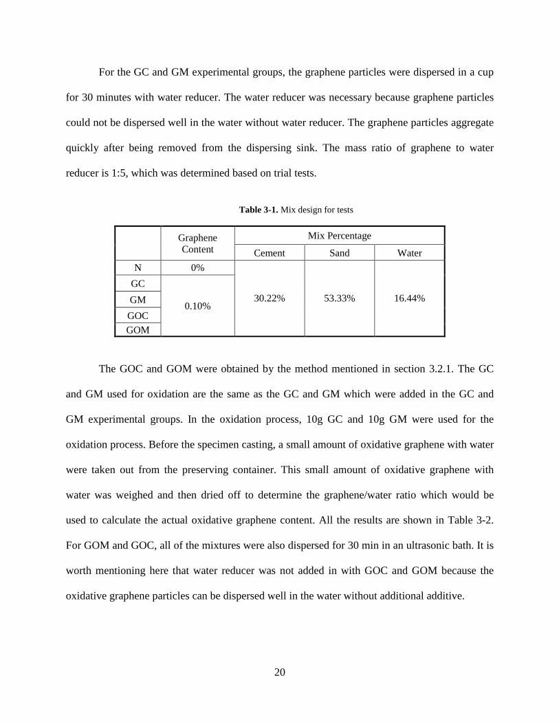
For the GC and GM experimental groups, the graphene particles were dispersed in a cup
for 30 minutes with water reducer. The water reducer was necessary because graphene particles
could not be dispersed well in the water without water reducer. The graphene particles aggregate
quickly after being removed from the dispersing sink. The mass ratio of graphene to water
reducer is 1:5, which was determined based on trial tests.
Table 3-1. Mix design for tests
Graphene Content
Mix Percentage
Cement Sand Water N 0%
30.22% 53.33% 16.44% GC
0.10% GM GOC GOM
The GOC and GOM were obtained by the method mentioned in section 3.2.1. The GC
and GM used for oxidation are the same as the GC and GM which were added in the GC and
GM experimental groups. In the oxidation process, 10g GC and 10g GM were used for the
oxidation process. Before the specimen casting, a small amount of oxidative graphene with water
were taken out from the preserving container. This small amount of oxidative graphene with
water was weighed and then dried off to determine the graphene/water ratio which would be
used to calculate the actual oxidative graphene content. All the results are shown in Table 3-2.
For GOM and GOC, all of the mixtures were also dispersed for 30 min in an ultrasonic bath. It is
worth mentioning here that water reducer was not added in with GOC and GOM because the
oxidative graphene particles can be dispersed well in the water without additional additive.

21
Table 3-2. Oxidative graphene content
Divided Mixture Total Mixture
Total Graphene Total Graphene GOC 3.5769 0.0825 400 9.2258g GOM 3.6382 0.0554 568 8.6491g
Then the specimens are ready to be cast. The dispersed graphene particles were added
into the water. Note: the total water content follows the mix design. The cement and sand were
premixed in the mixer, and then water and graphene were added in. The used cement is Type I
Portland cement. The fineness modulus of the used sand is 2.557. The sand sieve data is
documented in Appendix B3. The mixture was mixed in the mixer for 20 minutes and manual
mixed during the procedure to disintegrate some agglomerations. After casting the material in the
mould, the samples were vibrated for 5 minutes. Before de-molding, all the specimens sat for 24
hours with polyethylene film covering on the surface to prevent moisture loss. Every specimen
was cured in the moisture chamber (23°C, 100% humidity) for 28 days before the further use.
The composition of all the specimens is shown in Table 3-3.
Table 3-3. Specimen composition
Name Weight(g)
Graphene Water Reducer Cement Sand Water
N 0 0
9227.6 16284 5020.9 GC 9.2276 50 GM 9.2276 50 GOC 9.2258
0 GOM 8.6491

22
Figure 3-2. Casting procedure (a) cement and sand; (b) graphene with water; (c) mixer; and (d) specimen vibration
A total of 5 batches were cast, labelled as N, GM, GC, GOM and GOC based on
graphene particle used. Each batch has 3 cylinders, 12 cubes and 3 beams. Other specimen
information is shown in Table 3-4.
Figure 3-3. Specimens (1 batch): (a) fresh cast specimens and (b) 28-day cured specimens

23
Table 3-4. Specimen casting information
Name Specimen Volume(Liter)
Whole Volume
Batch Volume
Batch Weight 1.640 0.125 1.715
Cylinder Cube Beam N
3 12 3 11.57 L3 12.72 L3 30.53 kg GC GM
GOC GOM
3.3 TESTING
3.3.1 Trial tests
3.3.1.1 Compressive strength trial
In order to determine the graphene content in the experiments, a series of trial tests were
performed before the formal experiments. Several specimens were cast and tested for
compressive strength by using the TEST MARK CM4000 compression machine. All of the
specimens have the same mix proportion as mentioned in section 3.2.2, except the graphene
content. There are 7 groups of specimens with different graphene content for GC and GM. The
graphene content of these 7 groups of specimens are 0%, 0.1%, 0.2%, 0.4%, 1%, 2% and 4%,
respectively. The specimens are 5cm ×5cm × 5cm in size. Each group has 5 specimens except
the 1% and 4% graphene content groups. Because of the material availability, here only one
specimen was cast for the 1% and 4% groups. The tests results are shown in Table 3-5.

24
The results reveal that, for the GC specimens, the strength enhancements of all the
graphene additive specimens are about 10% higher than normal mortar. The strength
enhancement is relatively higher when graphene content is 0.2% and 1%. Among the GM
specimens, ones containing the 0.2% graphene content have the highest compressive strength.
When the graphene content is 2% and 4%, the strength of the specimens is less than the normal
mortar specimens. Considering the material availability and the trial tests results, the 0.1%
graphene content is chosen for the formal experiments.
Table 3-5. Compressive strength trial test results
Name Graphene Content
0% 0.1% 0.2% 0.4% 1% 2% 4%
GM
Specimen1 22400 22380 23810 21250
22760
20740
21240 Specimen2 22270 22320 25090 22390 20410
Specimen3 20510 21760 23460 24550 20120
Average 21726.67 22153.33 24120 22730 22760 20423.33 21240
Strength Comparison 1.96% 11.02% 4.62% 4.76% -6.00% -2.24%
GC
Specimen1 22400 25140 26000 23410
24980
24100
24620 Specimen2 22270 24430 23480 23610 24850
Specimen3 20510 24260 25350 24320 23680
Average 21726.67 24610 24943.33 23780 24980 24210 24620
Strength Comparison 13.27% 14.81% 9.45% 14.97% 11.43% 13.32%
3.3.1.2 Water absorption trial test
The water absorption trial tests of some specimens were also performed before the formal
experiments. After compressive tests, some broken specimens were smashed into small pieces to
make sure internal cracks did not exist. All the loosened particles were also eliminated from the
specimen surfaces. Before being put in the drying chamber for 48 hours, all of the samples were

25
submerged in the water for 24 hours and then were wiped to surface dry condition and then
weighed and marked. After drying, the specimens were weighed again, and the results are shown
in the Table 3-5.
Table 3-6. Water absorption strength trial test results
Graphene Content N GC GM GOC GOM 0% 12.70%
0.1% 12.80% 13.20% 12.80% 12.70% 0.2% 12.30% 12.10% 0.4% 12.40% 12.70%
Concerning the results, the water absorption ability of all the samples showed no
significant difference. The detailed test results could be found in Appendix A1.
3.3.2 Compressive strength test and Young's modulus & Poisson's ratio measurement
3.3.2.1 Introduction
Compressive strength, Young's modulus and Poisson's ratio are the basic parameters for
cementitious materials. In structural engineering, cementitious materials are always designed to
work under compression, and therefore the compressive strength is the key factor for a new
cementitious material. In addition, the Young's modulus and Poisson's ratio are necessary in
describing the mechanical property and prediction of the material behavior during the service.
Thus, this test was designed to compare the difference on the three material properties between
normal mortar and graphene reinforced mortar.
Here the specimens are cast in the shape of cylinders according to ASTM Standards. The
size is 10.16cm in radius and 20.23cm in height. Each group has three specimens, and all the

26
specimen were cast by the method which is described in the section 3.2.2 and were cured for 28
days.
3.3.2.2 Apparatus
The apparatus for this test are the Concrete Elastic Modulus Meter and the TEST MARK
CM4000 compression machine which are shown in Figure 3-4 (a) and (b).
Figure 3-4. Apparatus for compressive strength test and Young's Modulus & Poisson's Ratio measurement: (a)
Concrete Elastic Modulus Meter, (b) TEST MARK CM4000 compression machine
3.3.2.3 Test setup and procedure
The Concrete Elastic Modulus Meter is fixed on the specimen surface. The loading rate of the
TEST MARK was set to 440 lbs/s based on the ASTM standard.
Before the formal test, a trial-test was carried out on one specimen of the N group to
determinate the probable compressive strength. The test process for other specimens is divided

27
into three sequential steps. The first step is to preload to 10% of the compressive strength which
is estimated by the trial-test. All the loads were removed once the 10% of the compressive
strength was reached. The purpose of this step is to make sure the compression platforms have
full contact with the specimen. The second step is load to 40% of the compressive strength. All
the loads were removed once 40% of the compressive strength was reached. During this step, the
longitudinal and transverse dial gage readings were recorded as well as the corresponding
compressive force which is obtained from the loading machine. The Elastic Modulus Meter was
un-mounted from the specimen after this step. In the last step, the specimens were reloaded until
they were failed. The highest compressive forces were recorded for the compressive strength
calculation.
The stress was calculated as follows:
PSA
=
where: S is stress; P is applied load; and A is cross-sectional area of the cylindrical
specimen.
The strain was calculated as follows:
/ ogI Lε =
where:ε is strain; g is the longitudinal dial gage reading; oL is the length of the tested
area; and I is the reduction coefficient. Here, =0.5I .
The Young's modulus was calculated as follows:
2 1
2 0.000050S SE
ε−
=−
(ASTM C469)

28
where: E is chord modulus of elasticity, MPa; 2S is stress corresponding to 40% of
ultimate load; 1S is stress corresponding to a longitudinal strain, 1ε , of 50 millionths, MPa; and
2ε is longitudinal strain produced by stress 2S .
The Poisson's ratio was calculated as follows:
2 1
2 0.000050t tε εµ
ε−
=−
(ASTM C469)
where: µ is Poisson's ratio; 2tε is transverse strain at midheight of the specimen
produced by stress 2S ; 1tε is transverse strain at midheight of the specimen produced by stress
1S ; and 2ε is longitudinal strain produced by stress 2S .
3.3.3 Water absorption test
3.3.3.1 Introduction
The water absorption ability could generally reflect the porosity of the specimens. The porosity
of cementitious material is closely related with compressive strength, corrosion resistance, frost-
resistance and other material properties.
3.3.3.2 Apparatus
The water absorption test does not require sophisticated instrumentation. Only some containers
are needed for soaking the specimens. Besides, the drying chamber is needed to dry the
specimens.

29
3.3.3.3 Test setup and procedure
All the specimens were obtained from the compressive test which was presented in section 3.3.2.
The test setup and procedure is the same as the test which was mentioned in section 3.3.1.2.
3.3.4 Freezing and thawing test
3.3.4.1 Introduction
The freezing and thawing test is carried out here to investigate the frost resistance of the
graphene reinforced material. The parameters which were monitored during the process are the
specimen length and weight. The test procedure, test setup and test instruments were designed
based on the ASTM C666/C666M with some slight modifications according to the restrictions
on experimental equipment and materials. This test is still considered to be valuable and
objective because the conclusions and discussions of this test are based on comparing the
differences between the experimental groups and the control group.
The specimens are cast in the shape of beams with size = 7cm × 7cm × 35cm. Every
group has three specimens, and all the specimens were cast by the method which was described
in the section 3.2.2 and were cured in the moisture chamber for 28 days.
3.3.4.2 Apparatus
As shown in Figure 3-5, the equipment for the freezing and thawing test includes a 150cm (L) ×
75cm (W) × 30cm (H) water container, a GE 7.0 cubic ft. chest freezer and an electronic
thermometer. An electronic scale and an electronic slide caliper with calibrated precision were
also used for this test.
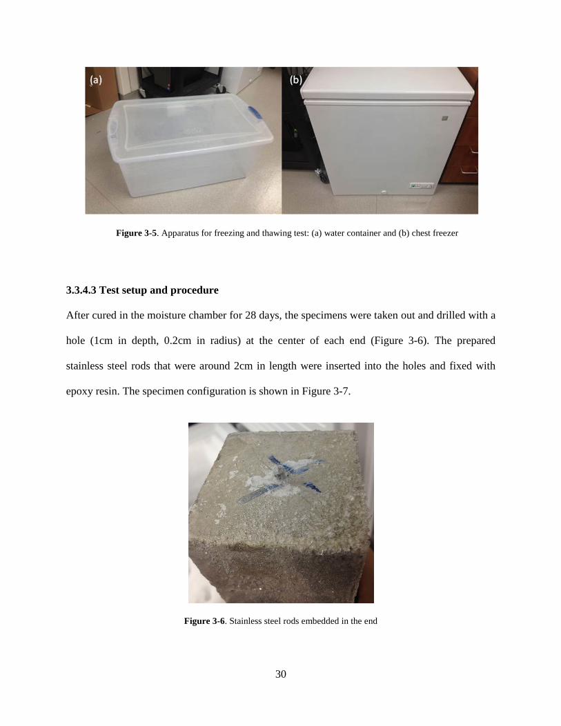
30
Figure 3-5. Apparatus for freezing and thawing test: (a) water container and (b) chest freezer
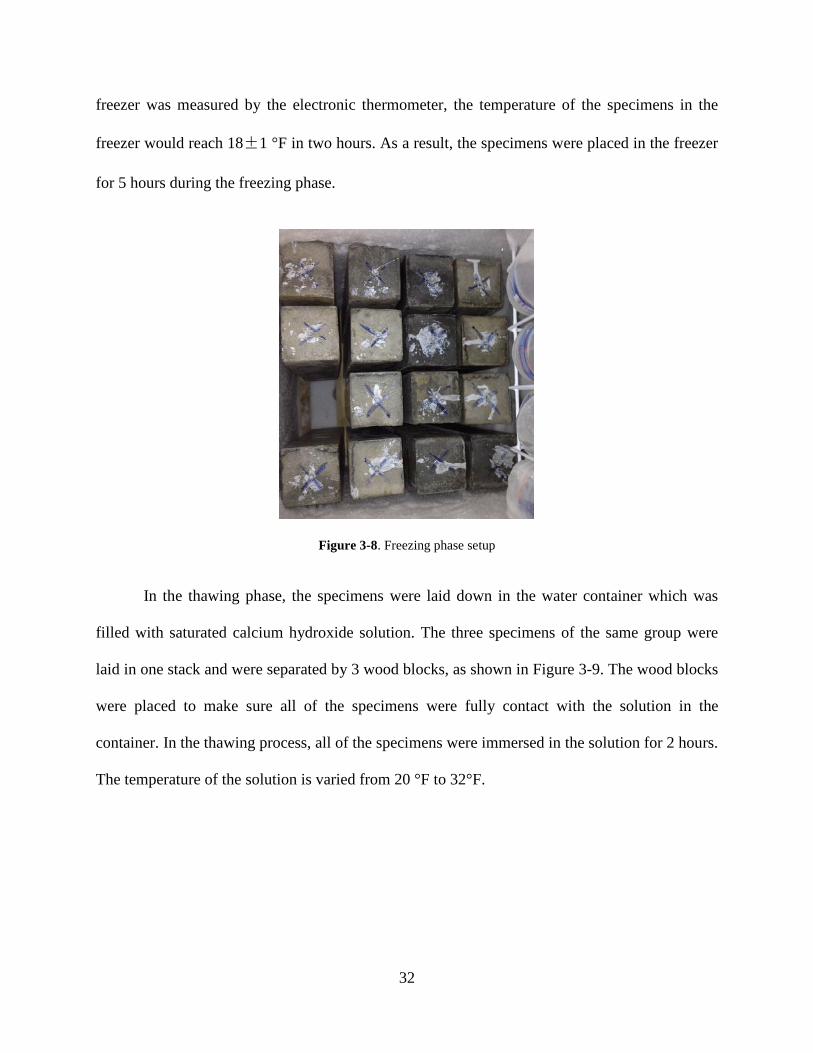
3.3.4.3 Test setup and procedure
After cured in the moisture chamber for 28 days, the specimens were taken out and drilled with a
hole (1cm in depth, 0.2cm in radius) at the center of each end (Figure 3-6). The prepared
stainless steel rods that were around 2cm in length were inserted into the holes and fixed with
epoxy resin. The specimen configuration is shown in Figure 3-7.
Figure 3-6. Stainless steel rods embedded in the end

31
The freezing and thawing test includes 300 cycles. Each cycle contains two phases:
freezing phase and thawing phase. For every cycle, the freezing phase was performed before the
thawing phase. All of the specimens were weighed and measured before the test cycles begin.
For every 26 cycles, each specimen was wiped to surface dry to weigh and measure for length
with the electronic scale and the electronic slide caliper, except the last cycle which has only 14
cycles. The specimens were weighed and measured for 13 times and all the experimental data
was recorded with the dates.
Figure 3-7. Specimen configuration
In freezing phase, the specimens were standing straight up in the chest freezer. In order to
make sure all of the specimens contact with the cold air, some wood battens were placed on the
bottom of the freezer, as shown in Figure 3-8. Because the temperature in the freezer is not
uniform from the top to the bottom, the specimens were placed on each end by turns. Thus, a "×"
symbol was marked on one end of every specimen (Figure 3-8). For the purpose of improving
the stability of the temperature in the freezer, several bottles of water were placed in the freezer 3
days before the test. These bottles of water were frozen into ice in two days and were preserved
in the freezer during the whole test. Their significant heat capacity could help to achieve constant
temperature during the freezing. Based on several trial tests in which the temperature in the
32
freezer was measured by the electronic thermometer, the temperature of the specimens in the
freezer would reach 18±1 °F in two hours. As a result, the specimens were placed in the freezer
for 5 hours during the freezing phase.
Figure 3-8. Freezing phase setup
In the thawing phase, the specimens were laid down in the water container which was
filled with saturated calcium hydroxide solution. The three specimens of the same group were
laid in one stack and were separated by 3 wood blocks, as shown in Figure 3-9. The wood blocks
were placed to make sure all of the specimens were fully contact with the solution in the
container. In the thawing process, all of the specimens were immersed in the solution for 2 hours.
The temperature of the solution is varied from 20 °F to 32°F.

33
Figure 3-9. Thawing phase setup
In the thawing phase, the specimens were laid down in the water container which was
filled with saturated calcium hydroxide solution. The three specimens of the same group were
laid in one stack and were separated by 3 wood blocks, as shown in Figure 3-9. The wood blocks
were placed to make sure all of the specimens were fully contact with the solution in the
container. In the thawing process, all of the specimens were immersed in the solution for 2 hours.
The temperature of the solution is varied from 20 °F to 32°F.
The weight change in percent was calculated as follows:
2 1c
1
100w wWw−
= ×
where: cW is weight change of the test specimen after C cycles of freezing and
thawing, %; 1w is weight of test specimen at 0 cycles; and 2w is weight of test specimen at C
cycles.
The weight change in percent was calculated as follows:
2 1c
1
100l lLl−
= ×

34
where: cL is weight change of the test specimen after C cycles of freezing and
thawing, %; 1l is measured length between 2 stainless steel rods of test specimen at 0 cycles; and
2l is measured length between 2 stainless steel rods of test specimen at C cycles.
3.3.5 Corrosion test
3.3.5.1 Introduction
In practice, the corrosion is one of the most common reasons for the destruction of concrete
structures, especially for reinforced concrete structures. The reinforcing steel bar inside the
concrete is susceptible to corrosion effect which lowers its strength level. However, the concrete
protective layer can effectively reduce the probability of corrosion of the internal steel bar.
Therefore, the corrosion resistance of concrete in reinforced concrete structures is particularly
important. This test is designed to investigate the corrosion resistance difference between normal
mortar and cementitious material reinforced by graphene.
The test method in this research is designed based on the study of Schneider and Chen
(2004). The specimens are cast in the shape of cube with size of 5cm × 5cm × 5cm. Each group
has 3 specimens. All of the specimens were cast by the method mention in Section 3.3.2.
3.3.5.2 Apparatus
As shown in Figure 3-10, the equipment used in this test includes a small water container which
has dimensions of 50cm (L) × 30cm (W) × 20cm (H) and the TEST MARK loading machine.
The chemical agents include ammonium nitrate, sodium hydroxide, phenolphthalein and
formaldehyde. All of these chemical agents were procured from Fisher Science Inc. To do the

35
acid-base neutralization titration and adding the solute, a burette and several beakers were also
needed.
Figure 3-10. Agents for corrosion test: (a) 15% ammonium nitrate solution; (b) ammonium nitrate; (c) burette; and
(d) sodium hydroxide solution, phenolphthalein and formaldehyde (from left to right)
3.3.5.3 Test setup and procedure
The highest ammonium nitrate concentration of the corrosion solution is 10% in Schneider and
Chen's (2004) research. Based on this, the concentration of ammonium nitrate in this study was
set to 15%. All of the specimens were directly immersed in 15% ammonium nitrate solution after
28 days curing. The specimens were taken out from the solution to do compression test after
corrosion for 1 month, 3 months and 5 months.
The stress of specimen was calculated as follows:

36
PSA
=
where: S is stress; P is applied load; and A is cross-sectional area of the cube specimen.
To maintain the concentration of ammonium nitrate of the solution, the concentration was
tested by acid-base neutralization titration and the ammonium nitrate was added into the solution
if the observed concentration is too low. The acid-base neutralization titrations were performed
as the following steps:
The titration records and the records of adding solute can be found in Appendix A2
1. Make 2.5 mol/L NaOH solution standby for the further step.
2. Take 25 mL NH4NO3 solution from the specimen container and keep in a beaker.
3. Add 17 mL formaldehyde into the beaker.
4. Add 2 drops of phenolphthalein into the beaker.
5. Use burette to add the NaOH solution into the beaker till the solution change to
red. Swirl the beaker after every few drops to mix well.
6. Read the Burette and calculate the concentration.

37
4.0 EXPERIMENTAL RESULTS AND DISCUSSION
This chapter reports the experimental records and results of the tests which are described in
chapter 3. The discussions of these results are also reported in this chapter.
4.1 COMPRESSIVE STRENGTH TEST AND YOUNG'S MODULUS & POISSON'S
RATIO MEASUREMENT
4.1.1 Results
The compressive strength, Young's modulus and Poisson ratio test records, calculations and
results are reported in the following sections. All of the results are calculated based on the
ASTM C39 (Compressive Strength of Cylindrical Concrete Specimens) and ASTM C469 (Static
Modulus of Elasticity and Poisson's Ratio of Concrete in Compression). The following tables
and figures are the test result summaries. The test records and calculations are shown in
Appendix A3.

38
Table 4-1. Compressive strength results
Compressive Strength (Mpa) Name Average Min Max %
N 34.59 31.37 37.53 GM 38.55 37.64 39.55 11.5% GC 41.48 38.93 43.17 19.9%
GOM 39.14 37.94 41.39 13.2% GOC 38.10 37.05 38.86 10.2%
Figure 4-1. Compressive strength results
Table 4-2. Young's modulus results
Young's Modulus (Gpa) Name Average Min Max %
N 17.00 16.97 17.02 GM 16.51 16.06 16.88 -2.9% GC 17.68 17.20 17.97 4.0%
GOM 16.98 16.86 17.11 -0.1% GOC 17.39 17.33 17.44 2.3%

39
Figure 4-2. Young's modulus results
Table 4-3. Poisson's ratio results
Poisson ratio Name Average Min Max %
N 0.1595 0.1543 0.1646 GM 0.1626 0.1615 0.1646 2.0% GC 0.1682 0.1572 0.1753 5.5%
GOM 0.1555 0.1446 0.1677 -2.5% GOC 0.1761 0.1750 0.1772 10.4%
Figure 4-3. Poisson's ratio results

40
4.1.2 Discussion
During the casting process of the trail tests and the formal tests, the graphene particles exhibit the
remarkable capacity to influence the liquidity and workability of cement paste. The graphene
particle additive mortar is more viscous than the normal mortar. This could be considered
evidence that the graphene nanoplatelets consumed the water in the cement composite because of
their high surface area.
The results of the compression strength test reveal that the strength increase of the GC
experimental group, about 20% compared to the control group, is higher than the other
experimental groups (Figure 4-1 and Table 4-1). In addition, the compressive strength of the
GOM group is 13.2% higher than that of the control group. The compressive strength increase of
the GM and GOC experimental groups are all about 10% compared to the control group.
As shown in Figure 4-2 and Table 4-2, the Young's modulus' results also show a similar
pattern. From the results, the Young's modulus of all the specimens are both 17.0±1.0 Gpa.
Thus, to some extent, the Young's modulus of the experimental groups can be regarded as not
having big differences. It is worth noting that, compared to the normal mortar group, the Young's
modulus of GC group is the highest in the experimental groups. As calculated in Table 4-2, the
Young's modulus of the GC group is 4% higher than the N group.
In the results of Poisson's ratio (Figure 4-3 and Table 4-3), the GOC group shows the
highest value (10.4% compared to the normal cement). In addition, the variation range of value
of three specimens of GOC group is smallest.

41
4.2 WATER ABSORPTION TEST
4.2.1 Results
The results of water absorption test could be found in Table 4-4 and Figure 4-4.
Table 4-4. Water absorption results
Name Soaked Weight (g)
48 hrs Dry Weight (g)
Water Content
N
73.1 64.8 12.8% 91.4 81.1 12.7% 66.9 59.2 13.0% 72.6 64.5 12.6%
Average 12.8%
GM
90.9 80.4 13.1% 91.5 80.8 13.2% 81.7 72.1 13.3% 49.7 43.8 13.5%
Average 13.3%
GC
72.3 64.3 12.4% 106.1 95.5 11.1% 66.3 59.1 12.2% 88.9 79.4 12.0%
Average 11.9%
GOM
81.3 72.1 12.8% 79.9 70.6 13.2% 62.1 55.0 12.9% 37.2 32.9 12.9%
Average 12.9%
GOC
97.6 86.6 12.7% 97.2 86.2 12.8% 72.5 63.9 13.5% 79.1 70.0 13.0%
Average 13.0%
42
Figure 4-4. Water absorption results
4.2.2 Discussion
As shown in Figure 4-4 and Table 4-4, the water content of GC groups is 11.92%, which is the
lowest value of all the experimental groups. The water content percent of other experimental
groups are both around 13%, and the GM group has the highest water content (13.27%). This
result reveals that, the porosity of the specimen is reduced because the presence of the C grade
graphene nanoplatelets. By comparing the GC with the GM experimental groups, it is found that
the grade C graphene is more effective than the grade M graphene on reducing the porosity.
Furthermore, the comparison between GM and GC experimental group is not affected by water
reducer, because the water reducer content is same in the GC group and GM group.

43
4.3 FREEZING AND THAWING TEST
4.3.1 Results
The test results summary is shown in the following figures. The detailed test records and
calculations of each specimen can be found in Appendix A4.
Figure 4-5. Weight change percentage of all the specimens

44
Figure 4-6. Average weight change percentage all the groups
Figure 4-7. Length change percentage of all the specimens

45
Figure 4-8. Average length change percentage of all the groups
4.3.2 Discussion
In this test, the weight change is monitored during the freezing and thawing cycles. For the GC
group, the specimens' weight increased at the first 130 cycles and decreased at the last 170 cycles.
The GOC group also shows the similar weight change record; however, the weight growing
phase of the GOC group (100 cycles) is shorter than this of GC group. Besides that, the extent of
weight growth of the GOC group is less than GC group.
Except the GC and the GOC group, the weight of the GOM, GM groups and the control
group are both decreased from the beginning. Among these three groups, the weight decrease of
the GOM group is the smallest.

46
The behaviors of the specimens' length were similar with the specimens' weight. The
percentages of length change of all the specimens are within 0.07%, except for the GC group, for
which the length increase reached 0.15% at the last cycles. The behaviors of increase are found
both in the GC and the GOC groups. But the amplitude of length increase of the GOC group is
less compared to the GC group. The largest length change of the GC group is 0.61 mm, while the
other specimens are around 0.2 mm.
On the other hand, the GOM group shows the lowest length change during the freezing
and thawing cycles. The average length change of the GOM group is within -0.04%. The
calculated results of weight and length change percentages can be found in Appendix A3.
The weight increase in the freezing and thawing test is considered as an abnormal
behavior. During the freezing and thawing cycles, the calcium hydroxide cannot cause the
weight gain because the concentration of calcium hydroxide inside the specimens is much higher
than that in the solution. The concentration of calcium hydroxide inside the specimens is high
because the calcium hydroxide is the main product of cement hydration. Therefore, the only
possibility for the weight gain of the GC and GOC groups is that water is preserved inside the
specimens. In the weight measurement, all of the specimens were only wiped to surface dry.
Thus, the weight of water inside the specimens was included in the results. Furthermore, the
spalling of specimens was rarely observed during the freezing and thawing cycles. Therefore, the
GC group showed the weight increase at the first 130 cycles.
It is also possible that the water preserving ability of the GC and GOC groups increased
because the internal tension cracks emerged. This conjecture is confirmed by the results of length
change. The length increase is generally considered as a sign of developing of tension cracks.
Actually, the ASTM standard says that if the expansions of the length exceed 0.1%, it means the

47
specimen failed to meet the requirement of the frost resistance. Thus, the performance of the GC
group in the freezing and thawing test is the worst.
Nevertheless, compared to the other groups, the GOM group showed the best
performance in the freezing and thawing cycles. The weight loss of the GOM group is lower than
the GM and N groups; the length change percentage of it is the smallest among all the groups.
4.4 CORROSION TEST
4.4.1 Results
The test results summary is shown in Table 4-5 and Figure 4-9. The detailed test records and
calculations can be found in Appendix A5.
Table 4-5. The average compressive strength test records of the N group
Stress(psi) N GC GM GOC GOM
28 Days
6263.33 6827.50 6122.50 6234.17 6592.50
Corrosion for 1
month 6546.67 6677.50 6315.83 6403.33 6166.25
Corrosion for 3
months 5629.17 5538.33 5275.83 5555.00 5951.25
Corrosion for 5
months 4885.00 5429.17 4410.83 4723.33 4950.00
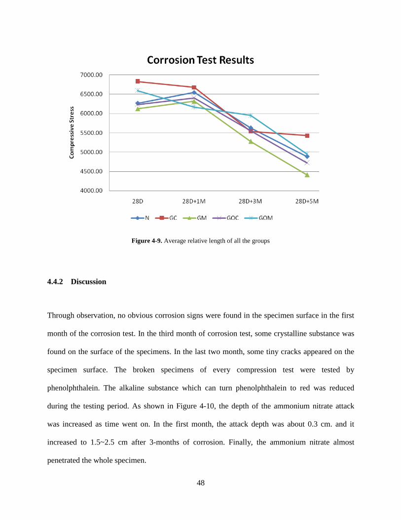
48
Figure 4-9. Average relative length of all the groups
4.4.2 Discussion
Through observation, no obvious corrosion signs were found in the specimen surface in the first
month of the corrosion test. In the third month of corrosion test, some crystalline substance was
found on the surface of the specimens. In the last two month, some tiny cracks appeared on the
specimen surface. The broken specimens of every compression test were tested by
phenolphthalein. The alkaline substance which can turn phenolphthalein to red was reduced
during the testing period. As shown in Figure 4-10, the depth of the ammonium nitrate attack
was increased as time went on. In the first month, the attack depth was about 0.3 cm. and it
increased to 1.5~2.5 cm after 3-months of corrosion. Finally, the ammonium nitrate almost
penetrated the whole specimen.

49
Figure 4-10. Specimens tested by phenolphthalein: (a) corrosion for 1 month; (b) 3 months; and (c) 5 months
The corrosion test result shows that the compressive strength of all the specimens is
weakened after 5-month corrosion. In the first month, the strength of the GC and GOM groups
dropped down while strength of the other groups rose up. In the second month and the third
month, the strength of all the specimens dropped down; furthermore, the dropping rate of the GC
group was the highest, and that of the GOM group was the lowest among all the other groups.
However, in the last two months, the strength dropping rate of the GC group was much lower
than the other groups. The results of the final compression test show that the compressive
strength of the GC and GOM groups is higher than the control group, while that of the GOC and
GM groups is lower than the control group.
The conclusion made by Lv et al. (2013) in their research may be used to explain the
specimen behavior in the corrosion test.
It is generally known that the mainly hydrates of hardened Portland cement are C-S-H
(3CaO·2SiO2·4H2O), calcium hydroxide (Ca(OH)2), ettringite (6CaO·Al2O3·3SO3·32H2O) and
calcium aluminum sulfate hydrate (4CaO·Al2O3·SO3·12H2O). Chen and Lei (2003) indicated
that NH4NO3 reacts with Ca(OH)2 and CaO of hydrates of Portland cement so that to damage the
composite structure of harden Portland cement. The reaction formulas are shown as follow:
Ca(OH)2 + NH4NO3 → Ca(NO3)2 + NH3↑ + H2O
CaO + NH4NO3 → Ca(NO3)2 + NH3↑ + H2O

50
Lv et al. suggested that the graphene reacts with Portland cement. They also indicated
that ettringite is less prevalent in the hydrates because of the reaction between graphene and
cement. Lv et al. also concluded that the reaction between graphene and Portland cement is an
endothermic reaction which can reduce the thermal cracks during the hydration process,
enhancing the strength of the specimen.
Based on this, the reasonable speculation is: the ettringite in the GC group's specimens is
less than the other specimens because the GC group shows the highest compressive strength in
section 4.1.1. Therefore, the strength dropping rate of the GC group is slightly faster than the
other groups in the first three months. Another conjecture is GC can accelerate the hydration
process during the 28-day curing. Thus strength of GC group dropped down at the beginning of
the corrosion; while the strength of the other groups slightly grew up because of the continuous
hydration.
Chen and Lei (2003) also indicate that the reaction product Ca(NO3)2 can continuously
react with Ca(OH)2, producing Ca(NO3)2·H2O which is a large crystal. The growth of this crystal
inside the microcracks and cavities of hardened Portland cement can cause expansion stress so
that to further damage the cement. Therefore, the GC group which has fewer microcracks
resisted the corrosion better than the other groups, so that the GC group exhibited the highest
compressive strength at the end.

51
5.0 MICROSCOPIC PROBE
This chapter shows the microscope observations of the cementitious material samples. The
microscopic approaches include atomic force microscope (AFM) observation, Raman
spectroscopy test and scanning electron microscope (SEM) observation. This chapter also
discusses the results of these probe methods.
5.1 SPECIMEN PREPARATION
5.1.1 Specimen casting
The specimens for microscopic observation were both cut from broken pieces of the compression
test, as describes in section 3.3.2. The broken pieces were cut into small blocks with dimensions:
10mm (L) × 5mm (W) × 5mm (T). Each sample was polished by the 150 grade sand paper to
smoothen the surface. Every group has one sample. All of the polished samples were cast in the
plastic rings with epoxy resin and then were dried in the drying chamber for 24 hours. As shown
in Figure 5-1, three samples were cast in the same ring so that to reduce the polishing workload
in the next step.
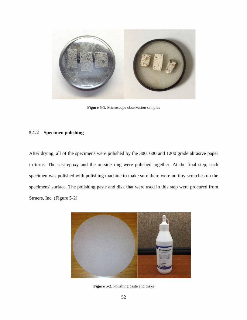
52
Figure 5-1. Microscope observation samples
5.1.2 Specimen polishing
After drying, all of the specimens were polished by the 300, 600 and 1200 grade abrasive paper
in turns. The cast epoxy and the outside ring were polished together. At the final step, each
specimen was polished with polishing machine to make sure there were no tiny scratches on the
specimens' surface. The polishing paste and disk that were used in this step were procured from
Struers, Inc. (Figure 5-2)
Figure 5-2. Polishing paste and disks

53
5.2 ATOMIC FORCE MICROSCOPE OBSERVATION
5.2.1 Test instrumentation and setup
The device used for this test is the Veeco Manifold Multimode V& Dimension V scanning probe
microscopy (Figure 5-3). By combining the Multimode V SPM and the Dimension V SPM with
several advanced application modules, the manifold SPM combination offers atomic force
microscopy observation. (PINSE, 2014) The tapping mode was used in the test and the scan rate
is set to 0.5 Hz. The samples used in this test were prepared by the method that mentioned in
section 5.1.
Figure 5-3. Atomic force microscope (PINSE, 2014)

54
5.2.2 Results and discussion
The images obtained by the AFM of all the samples are shown in Figure 5-4~8. The scan areas
of N, GC and GM samples are 2.0 μm. The scan areas of GOC and GOM samples are 300 nm.
Figure 5-4. The N sample's image obtained by AFM
Figure 5-5. The GM sample's image obtained by AFM

55
Figure 5-6. The GC sample's image obtained by AFM
Figure 5-7. The GOM sample's image obtained by AFM

56
Figure 5-8. The GOC sample's image obtained by AFM
These images were obtained from AFM by scanning the interested points on the
specimen surface. The interested points were black particles or with other features that graphene
was possibly embedded.
Based on the research of Alkhateb (Alkhateb et al. 2013), the variation in the C-S-H
distribution and packing could be disturbed because of the presence of the graphene
nanoplatelets. More specifically, the surface of graphene should be smoother than that of C-S-H.
However, from the results of this test, the surfaces of all the samples are both exhibit a relatively
coarse topography, except the images of GC sample. Even though the topography in the image is
relatively flat and smooth as shown in Figure 5-6, the conclusion cannot be determined that
graphene is embedded in the observed surfaces. Therefore, before the AFM observations, other
approaches should be performed to roughly locate the graphene particles.

57
5.3 RAMAN SPECTROSCOPY TEST
5.3.1 Test instrumentation
As shown in Figure 5-9, the Renishaw inVia Raman microscope is used in this test.
Figure 5-9. Renishaw inVia Raman microscope (PINSE, 2014)
5.3.2 Results and discussion
In this test, the pristine GM and the sample of GM was tested. Figure 5-10 shows the results of
pristine GM. The peak waves of Raman shift are presented around 1600 cm-1 and 2600 cm-1.
This result is similar to the Raman spectroscopy of GM which is provided by XG Sciences, Inc.
Because the particularity of graphene Raman spectrum, the location of the graphene can be
determined by the following steps. First, use optical microscope to roughly locate a point that
may be graphene particles on the sample's surface. Secondly, induce the red laser to precisely
locate the interested point on the sample. Next, perform Raman spectrum scan and analyze the

58
results. If the results exhibit peak waves around 1600 cm-1 and 2600 cm-1 (Figure 5-11), it means
this point should be graphene. Finally, record the optical microscope image (Figure 5-12) with
the Raman spectroscopy results. Some Raman spectroscopy images obtained in this test can be
found in Appendix B2.
Figure 5-10. Raman spectroscopy observation results of GM
Figure 5-11. Raman spectroscopy results of GC cement sample
Figure 5-12. Optical microscope image of GC cement sample
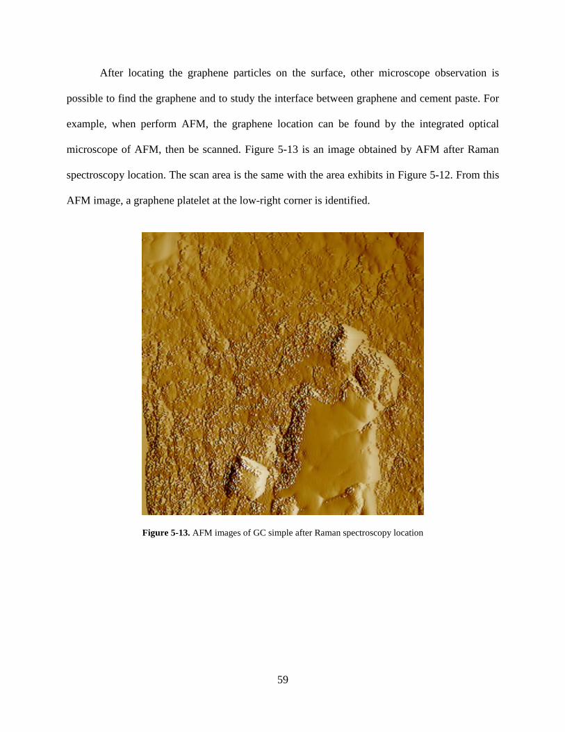
59
After locating the graphene particles on the surface, other microscope observation is
possible to find the graphene and to study the interface between graphene and cement paste. For
example, when perform AFM, the graphene location can be found by the integrated optical
microscope of AFM, then be scanned. Figure 5-13 is an image obtained by AFM after Raman
spectroscopy location. The scan area is the same with the area exhibits in Figure 5-12. From this
AFM image, a graphene platelet at the low-right corner is identified.
Figure 5-13. AFM images of GC simple after Raman spectroscopy location
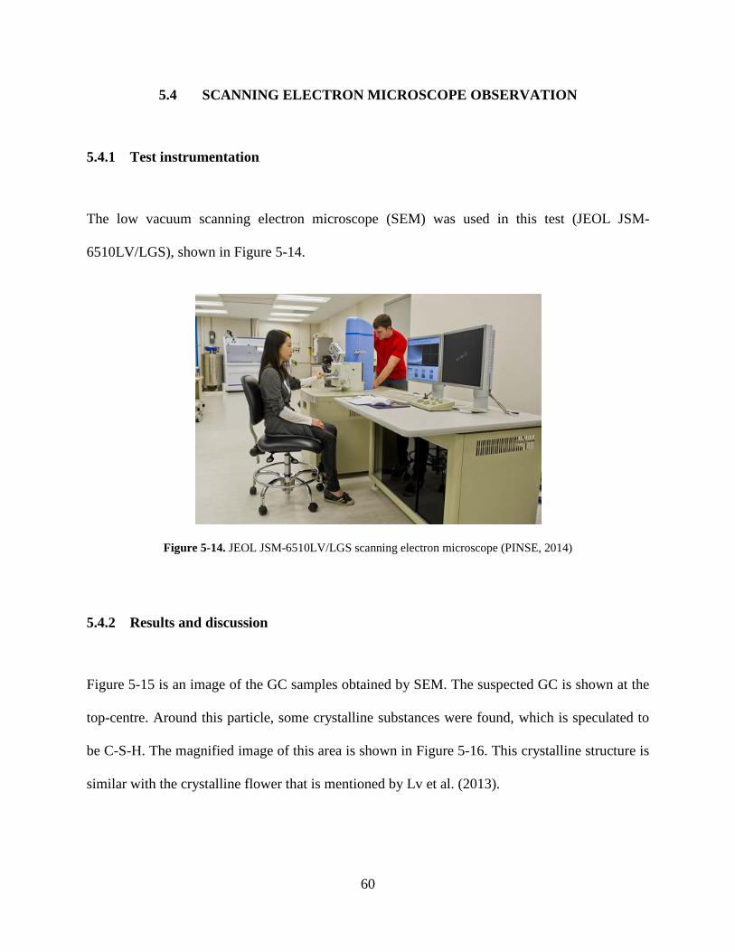
60
5.4 SCANNING ELECTRON MICROSCOPE OBSERVATION
5.4.1 Test instrumentation
The low vacuum scanning electron microscope (SEM) was used in this test (JEOL JSM-
6510LV/LGS), shown in Figure 5-14.
Figure 5-14. JEOL JSM-6510LV/LGS scanning electron microscope (PINSE, 2014)
5.4.2 Results and discussion
Figure 5-15 is an image of the GC samples obtained by SEM. The suspected GC is shown at the
top-centre. Around this particle, some crystalline substances were found, which is speculated to
be C-S-H. The magnified image of this area is shown in Figure 5-16. This crystalline structure is
similar with the crystalline flower that is mentioned by Lv et al. (2013).

61
Figure 5-15. SEM images of GC sample
Figure 5-16. SEM images of GC sample

62
6.0 SUMMARY, CONCLUSIONS, AND RECOMMENDATIONS
6.1 SUMMARY
This research presented a series of experiments to investigate the properties of cementitious
material which is reinforced by graphene nanoplatelets. All the specimens were casted and cured
based on the ASTM C192/C192M "Standard Practice for Making and Curing Concrete Test
Specimens in the Laboratory". The curing time of all of the specimens was 28 days.
In the compressive strength and Young's modulus & Poisson's ratio test, a total of fifteen
specimens were tested based on ASTM C469/C469M "Standard Test Method for Static Modulus
of Elasticity and Poisson's Ratio of Concrete in Compression". The broken pieces were used to
determine water absorption by measuring soaked weight and dry weight.
The freezing and thawing tests were also performed in this research. Every specimen was
experienced 300 freezing thawing cycles. The mass weight loss and specimen length were
measured each 26 cycles. The test procedure and condition were designed and modified based
upon ASTM C666/C66M "Standard Test Method for Resistance of Concrete to Rapid Freezing
and Thawing".
A total of 60 specimens were tested in corrosion experiment. After curing for 28 days,
every specimen is placed in 15% ammonium nitrate solution for 5 months. The first 15

63
specimens were tested for 28-days compressive strength. Each 15 specimens were tested at 1
month, 3 months and 5 months corrosion period.
To explore the mechanism of mechanical properties enhancement caused by graphene,
the atomic force microscopy, Raman spectroscopy and scanning electron microscopy
observation were performed.
6.2 CONCLUSIONS
Based on the literature review and the test results, the conclusions are made as follows:
1. The GC, GOM, GM and GOC can improve the compressive strength of cementitious
materials. The compressive strength of them is 19.9%, 13.2%, 11.5% and 10.2% higher
than the normal mortar, respectively.
2. The GC can effectively improve the water preserving ability of cementitious materials
and thus it will weaken the frost resistance of harden Portland cement, whereas the GOM
can slightly improve the frost resistance of cementitious materials.
3. The corrosion resistance of cementitious materials within 5 months can be boosted by the
GC and GOM, while this can be weakened by the GM. From the current experimental
data, the GC and GOM are more likely to raise long-term acid corrosion resistance of
concrete.
4. Nitric acid oxidation of graphene nanoplatelets on improving the cementitious material
strength is not as good as expected. However, the oxidation treatment is necessary
because it can mitigate the detrimental effect of plain graphene particles on frost
resistance of cementitious materials.

64
5. The performance of the GOM group is best among all the experimental groups, by
comprehensive consideration of all the experimental results
6. The Raman spectroscopy observation is powerful when locating graphene nanoplatelets
in the cement surface. It can help the researchers to locate the graphene in AFM
observation to make the images obtained in AFM are more credible rather than only
judging the existing of graphene by topography.
6.3 RECOMMENDATIONS
This research is presented with limited experimental conditions and materials. It can be improved
in several aspects. In addition, the mechanism of improvement of cementitious material caused
by graphene is still unclear. Thus, the further studies are needed. There are some
recommendations for the future studies:
1. The small size graphene nanoplatelet exhibits more effective capacity to improve the
compressive strength of the cementitious materials than the big one. To reach higher
compressive strength, the small size graphene is recommended, such as the graphene
platelets used by Sedaghat et al. (2013). Its dimension is only 110 × 110 × 0.12 nm
(Angstrom Materials, N008-100-N). In addition, it is better to set more experimental
groups with different graphene platelet sizes.
2. Continue research on how to improve the frost resistance of C grade graphene additive
cement, such as adding air entraining agent in to the mix proportion design.
3. Try other oxidation treatment method of graphene particles, such as the method presented
by Lv et al. (2013).
65
4. Adopt freezing thawing chamber for the freezing and thawing test. It can improve the
stability of the freezing and thawing cycles so to reduce the experiment error.
Furthermore, employ relative dynamic modulus loss as a criterion to evaluate the frost
resistance.
5. Add more types of corrosive solution in the corrosion test to perform contrast
experiments and advisably elongate the corrosion period.
6. Perform nano indentation tests by using AFM to measure the micro modulus of the
specimens. The researching area should be focused at the interface between the graphene
platelet and C-S-H.
7. Molecular dynamics simulation is helpful to research the mechanism of enhancement of
cementitious materials by graphene nanoplatelets.

66
APPENDIX A
A.1 TRIAL WATER ABSORPTION RESULTS RECORD
Table A-1. Test results of water absorption trial test: N
Soaked Weight 48 hrs Dry Weight Water Content
N
120.4 107.3 12.2% 135.5 119.8 13.1% 96.8 85.8 12.8%
Average 12.7%
Table A-2. Test results of water absorption trial test: 0.1% GC
Soaked Weight 48 hrs Dry Weight Water Content
0.1% GC
90.0 79.5 13.2% 75.4 67.0 12.5% 81.0 71.9 12.7% 92.0 81.5 12.9%
Average 12.8%
Table A-3. Test results of water absorption trial test: 0.1% GM
Soaked Weight 48 hrs Dry Weight Water Content
0.1% GM
68.1 60.1 13.3% 85.8 75.8 13.2% 70.6 62.4 13.1% 85.5 75.6 13.1%
Average 13.2%

67
Table A-4. Test results of water absorption trial test: 0.1% GOC
Soaked Weight 48 hrs Dry Weight Water Content
0.1% GOC
92.1 81.8 12.6% 75.2 66.7 12.7% 75.5 66.7 13.2%
Average 12.8%
Table A-5. Test results of water absorption trial test: 0.1% GOM
Soaked Weight 48 hrs Dry Weight Water Content
0.1% GOM
92.4 82.8 11.6% 84.3 74.0 13.9% 98.2 87.4 12.4% 77.1 68.3 12.9%
Average 12.7%
Table A-6. Test results of water absorption trial test: 0.2% GC
Soaked Weight 48 hrs Dry Weight Water Content
0.2% GC
55.6 49.4 12.6% 109.2 97.1 12.5% 93.2 83.3 11.9%
Average 12.3%
Table A-7. Test results of water absorption trial test: 0.2% GM
Soaked Weight 48 hrs Dry Weight Water Content
0.2% GM
81.6 73.2 11.5% 99.4 87.1 14.1% 93.4 83.8 11.5% 90.1 80.8 11.5%
Average 12.1%

68
Table A-8. Test results of water absorption trial test: 0.4% GC
Soaked Weight 48 hrs Dry Weight Water Content
0.4% GC
103.4 92.5 11.8% 97.9 86.3 13.4% 90.3 80.3 12.5% 61.5 55.0 11.8%
Average 12.4%
Table A-9. Test results of water absorption trial test: 0.4% GM
Soaked Weight 48 hrs Dry Weight Water Content
0.4% GM
83.7 74.9 11.7% 95.1 84.7 12.3% 90.7 80.0 13.4% 63.9 56.4 13.3%
Average 12.7%
A.2 TITRATION RECORDS
Table A-10. Titration records before the first compression test
28 Days + 1 Month
Date Quantity of used NaOH solution(mL) Concentration Jul. 15 19.2 15.36% Jul. 16 16.3 13.04% Jul. 17 16.3 13.04% Jul. 17 Add 196g Jul. 18 17.7 14.16% Jul. 19 17.1 13.68% Jul. 22 16.6 13.28% Jul. 22 Add 172g Jul. 24 16.6 13.28% Jul. 26 15.8 12.64% Jul. 26 Add 236g Jul. 31 16.1 12.88% Jul. 31 Add 212g
Aug. 09 16.9 13.52% Aug. 13 15.6 12.48%

69
Table A-11. Titration records before the second compression test
28 Days + 3 Months
Date Quantity of used NaOH solution(mL) Concentration Aug. 15 15.3 12.24% Aug. 15 Add 276g Aug. 28 15.5 12.40% Aug. 28 Add 260g Sept. 09 16.8 13.44% Sept. 16 15.8 12.64% Sept. 23 15.1 12.08% Sept. 23 Add 292g Sept. 30 17.6 14.08% Oct. 07 16.8 13.44% Oct. 14 16.1 12.88% Oct. 14 Add 212g
Table A-12. Titration records before the last compression test
28 Days + 5 Months
Date Quantity of used NaOH solution(mL) Concentration Oct. 21 17.8 14.24% Oct. 28 17.2 13.76% Nov. 04 16.7 13.36% Nov. 11 16.2 12.96% Nov. 11 Add 204g Nov. 18 18.1 14.48% Nov. 25 17.4 13.92% Dec. 02 16.9 13.52% Dec. 09 16.7 13.36% Dec. 14 16.3 13.04% Dec. 14 Add 196g

70
A.3 TESTS RECORDS OF COMPRESSIVE STRENGTH TEST AND YOUNG'S
MODULUS & POISSON'S RATIO MEASUREMENT
Table A-13. Compressive strength records and calculations of the N group
F(lbs) Area(mm²) Strength(MPa) N1 57220 8107.32 31.37 N2 68440 8107.32 37.53 N3 63580 8107.32 34.86
Average 34.59
Table A-14. Young's modulus records and calculations of the N group
0.005 0.005 Force End End
Force Stress Strain E
N1 - - - - - - - N2 0.0125 2680 0.1390 22000 10.59 0.000622539 17015.81 N3 0.0050 1080 0.1620 25000 13.12 0.000772638 16974.52
Average 16995.16
Table A-15. Poisson's ratio records and calculations of the N group
Force Long. DSPL Tran. DSPL Poisson's's
ratio Average
N1
0.15394
N2
2680 0.0125 0.0030 0.2400 4980 0.0254 0.0050 0.1969 6980 0.0381 0.0070 0.1837 8910 0.0508 0.0090 0.1772
13040 0.0762 0.0130 0.1706 22000 0.1397 0.0230 0.1646
N3
1080 0.0050 0.0000 0.0000 3440 0.0200 0.0020 0.1000 6880 0.0400 0.0060 0.1500
10200 0.0600 0.0090 0.1500 16600 0.1000 0.0160 0.1600 25000 0.1620 0.0250 0.1543

71
Table A-16. Compressive strength records and calculations of the GM group
F(lbs) Area(mm²) Strength(MPa) GM1 72130 8107.32 39.55 GM2 68650 8107.32 37.64 GM3 70130 8107.32 38.45
Average 38.55
Table A-17. Young's modulus records and calculations of the GM group
0.005 0.005 Force End End
Force Stress Strain E
GM1 0.0400 6690 0.1670 25000 10.04 0.000625 16062.78 GM2 0.0200 3770 0.1640 25200 11.75 0.000708661 16580.42 GM3 0.0050 1470 0.1610 25100 12.96 0.000767717 16876.22
Average 16506.47
Table A-18. Poisson's ratio records and calculations of the GM group
Force Long. DSPL Tran. DSPL Poisson's
ratio Average
GM1
0 0.0000 0.0000 0.0000
0.16260
0 0.0000 0.0000 0.0000 6690 0.0400 0.0070 0.1750 9890 0.0600 0.0100 0.1667
16050 0.1000 0.0170 0.1700 25000 0.1670 0.0270 0.1617
GM2
0 0.0000 0.0000 0.0000 3770 0.0200 0.0030 0.1500 6960 0.0400 0.0070 0.1750
10300 0.0600 0.0100 0.1667 16590 0.1000 0.0160 0.1600 25000 0.1640 0.0270 0.1646
GM3
1470 0.0050 0.0010 0.2000 3780 0.0200 0.0030 0.1500 7160 0.0400 0.0040 0.1000
10030 0.0600 0.0090 0.1500 16780 0.1000 0.0160 0.1600 25100 0.1610 0.0260 0.1615

72
Table A-19. Compressive strength records and calculations of the GC group
F(lbs) Area(mm²) Strength(MPa) GC1 78730 8107.32 43.17 GC2 71000 8107.32 38.93 GC3 77230 8107.32 42.34
Average 41.48
Table A-20. Young's modulus records and calculations of the GC group
0.005 0.005 Force End End
Force Stress Strain E
GC1 0.0050 1220 0.1590 25000 13.04 0.000757874 17203.91 GC2 0.0050 1460 0.1510 25010 12.91 0.000718504 17971.07 GC3 0.0050 1400 0.1540 25300 13.10 0.000733268 17870.95
Average 17681.98
Table A-21. Poisson's ratio records and calculations of the GC group
Force Long. DSPL Tran. DSPL Poisson's
ratio Average
GC1
1220 0.0050 0.0000 0.0000
0.16825
3610 0.0200 0.0030 0.1500 6980 0.0400 0.0060 0.1500
10260 0.0600 0.0100 0.1667 16350 0.1000 0.0160 0.1600 25000 0.1590 0.0250 0.1572
GC2
1460 0.0050 0.0010 0.2000 4130 0.0200 0.0040 0.2000 7760 0.0400 0.0070 0.1750
11570 0.0600 0.0110 0.1833 17520 0.1000 0.0180 0.1800 25010 0.1510 0.0260 0.1722
GC3
1400 0.0050 0.0010 0.2000 4130 0.0200 0.0040 0.2000 7390 0.0400 0.0070 0.1750
10740 0.0600 0.0110 0.1833 17230 0.1000 0.0180 0.1800 25300 0.1540 0.0270 0.1753

73
Table A-22. Compressive strength records and calculations of the GOM group
F(lbs) Area(mm²) Strength(MPa) GOM1 69200 8107.32 37.94 GOM2 75480 8107.32 41.39 GOM3 69450 8107.32 38.08
Average 39.14
Table A-23. Young's modulus records and calculations of the GOM group
0.005 0.005 Force End End
Force Stress Strain E
GOM1 0.0050 940 0.1660 25300 13.36 0.000792323 16857.27 GOM2 0.0050 1100 0.1620 25000 13.10 0.000772638 16960.33 GOM3 0.0050 1090 0.1610 25050 13.14 0.000767717 17111.90
Average 16976.50
Table A-24. Poisson's ratio records and calculations of the GOM group
Force Long. DSPL Tran. DSPL Poisson's
ratio Average
GOM1
940 0.0050 0.0000 0.0000
0.15553
3460 0.0200 0.0025 0.1250 6690 0.0400 0.0050 0.1250 10120 0.0600 0.0075 0.1250 16070 0.1000 0.0125 0.1250 25300 0.1660 0.0240 0.1446
GOM2
1100 0.0050 0.0010 0.2000 3470 0.0200 0.0030 0.1500 6820 0.0400 0.0070 0.1750 10310 0.0600 0.0100 0.1667 16380 0.1000 0.0160 0.1600 25000 0.1620 0.0250 0.1543
GOM3
1090 0.0050 0.0010 0.2000 3810 0.0200 0.0040 0.2000 7000 0.0400 0.0070 0.1750 10530 0.0600 0.0100 0.1667 16420 0.1000 0.0160 0.1600 25050 0.1610 0.0270 0.1677

74
Table A-25. Compressive strength records and calculations of the GOC group
F(lbs) Area(mm²) Strength(MPa) GOC1 67570 8107.32 37.05 GOC2 70040 8107.32 38.40 GOC3 70880 8107.32 38.86
Average 38.10
Table A-26. Young's modulus records and calculations of the GOC group
0.005 0.005 Force End End
Force Stress Strain E
GOC1 0.0050 1060 0.1590 25020 13.14 0.000757874 17334.13 GOC2 0.0050 970 0.1600 25190 13.28 0.000762795 17409.18 GOC3 0.0050 1330 0.1580 25280 13.13 0.000752953 17440.14
Average 17394.49
Table A-27. Poisson's ratio records and calculations of the GOC group
Force Long. DSPL Tran. DSPL Poisson's
ratio Average
GOC1
1060 0.0050 0.0010 0.2000
0.17611
3690 0.0200 0.0040 0.2000 6990 0.0400 0.0080 0.2000 10390 0.0600 0.0120 0.2000 16630 0.1000 0.0180 0.1800 25020 0.1590 0.0280 0.1761
GOC2
1190 0.0050 0.0010 0.2000 2210 0.0200 0.0300 1.5000 3210 0.0400 0.0070 0.1750 7610 0.0600 0.0110 0.1833 11090 0.1000 0.0180 0.1800 14430 0.1600 0.0280 0.1750
GOC3
1310 0.0050 0.0001 0.0200 2280 0.0200 0.0040 0.2000 3180 0.0400 0.0070 0.1750 4120 0.0600 0.0110 0.1833 7810 0.1000 0.0180 0.1800 11270 0.1580 0.0280 0.1772

75
Figure A-1. Compressive force vs. longitudinal displacement of the N group
Figure A-2. Compressive force vs. longitudinal displacement of the GM group

76
Figure A-3. Compressive force vs. longitudinal displacement of the GC group
Figure A-4. Compressive force vs. longitudinal displacement of the GOM group
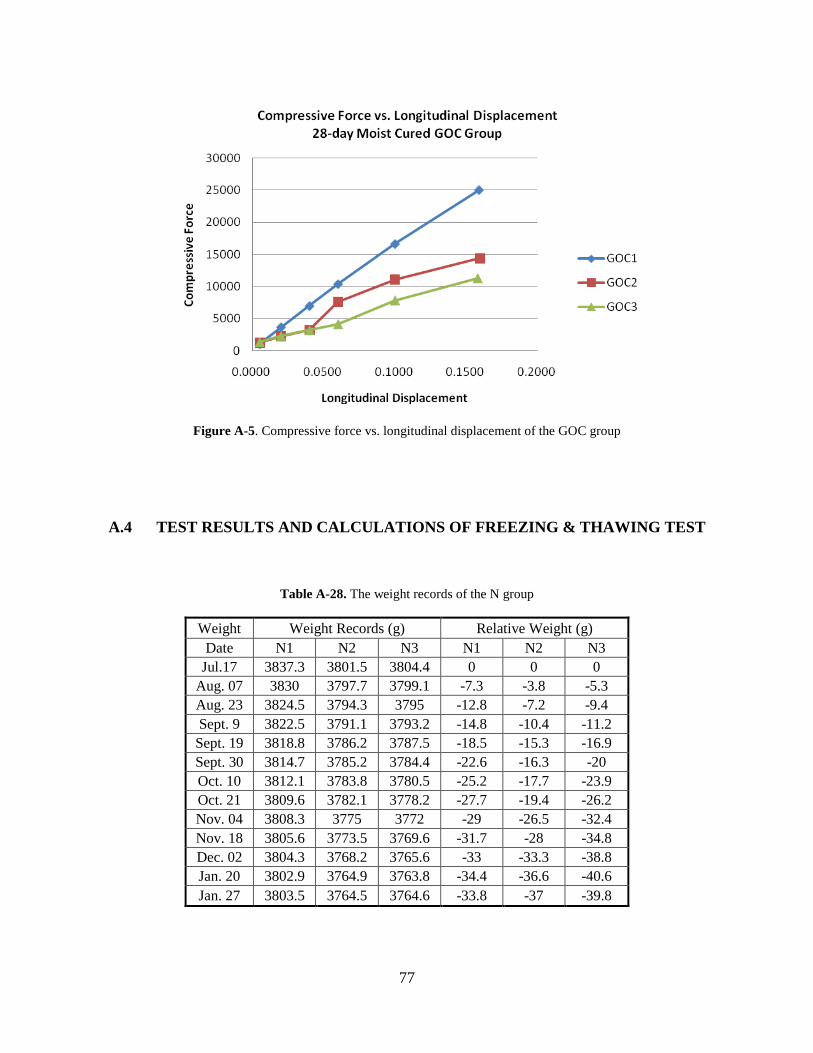
77
Figure A-5. Compressive force vs. longitudinal displacement of the GOC group
A.4 TEST RESULTS AND CALCULATIONS OF FREEZING & THAWING TEST
Table A-28. The weight records of the N group
Weight Weight Records (g) Relative Weight (g) Date N1 N2 N3 N1 N2 N3
Jul.17 3837.3 3801.5 3804.4 0 0 0 Aug. 07 3830 3797.7 3799.1 -7.3 -3.8 -5.3 Aug. 23 3824.5 3794.3 3795 -12.8 -7.2 -9.4 Sept. 9 3822.5 3791.1 3793.2 -14.8 -10.4 -11.2 Sept. 19 3818.8 3786.2 3787.5 -18.5 -15.3 -16.9 Sept. 30 3814.7 3785.2 3784.4 -22.6 -16.3 -20 Oct. 10 3812.1 3783.8 3780.5 -25.2 -17.7 -23.9 Oct. 21 3809.6 3782.1 3778.2 -27.7 -19.4 -26.2 Nov. 04 3808.3 3775 3772 -29 -26.5 -32.4 Nov. 18 3805.6 3773.5 3769.6 -31.7 -28 -34.8 Dec. 02 3804.3 3768.2 3765.6 -33 -33.3 -38.8 Jan. 20 3802.9 3764.9 3763.8 -34.4 -36.6 -40.6 Jan. 27 3803.5 3764.5 3764.6 -33.8 -37 -39.8

78
Figure A-6. The weight records of the N group
Table A-29. The weight records of the GM group
Weight Weight Records (g) Relative Weight (g) Date GM1 GM2 GM3 GM1 GM2 GM3
Jul.17 3865.7 3841 3840.4 0 0 0 Aug. 07 3858.2 3830.4 3831.9 -7.5 -10.6 -8.5 Aug. 23 3852.5 3822.9 3824.7 -13.2 -18.1 -15.7 Sept. 9 3849.8 3817.8 3819.8 -15.9 -23.2 -20.6
Sept. 19 3843.5 3812.6 3814.8 -22.2 -28.4 -25.6 Sept. 30 3839.2 3809.5 3809.8 -26.5 -31.5 -30.6 Oct. 10 3836.3 3807.1 3807.2 -29.4 -33.9 -33.2 Oct. 21 3835.1 3805.2 3804.6 -30.6 -35.8 -35.8 Nov. 04 3829.9 3801.7 3801.8 -35.8 -39.3 -38.6 Nov. 18 3826.5 3800.9 3799.7 -39.2 -40.1 -40.7 Dec. 02 3825 3794.8 3796.6 -40.7 -46.2 -43.8 Jan. 20 3821.2 3793.3 3793.2 -44.5 -47.7 -47.2 Jan. 27 3820.3 3792.3 3794.6 -45.4 -48.7 -45.8

79
Figure A-7. The weight records of the GM group
Table A-30. The weight records of the GC group
Weight Weight Records (g) Relative Weight (g)
Date GC1 GC2 GC3 GC1 GC2 GC3 Jul.17 3849.4 3884.7 3837.4 0 0 0
Aug. 07 3850.1 3889.6 3841.4 0.7 4.9 4 Aug. 23 3854.4 3893.7 3846.2 5 9 8.8 Sept. 9 3858.6 3895.1 3849.8 9.2 10.4 12.4 Sept. 19 3858.6 3896.3 3850.2 9.2 11.6 12.8 Sept. 30 3860.6 3896.7 3851.6 11.2 12 14.2 Oct. 10 3858.5 3895.7 3851.5 9.1 11 14.1 Oct. 21 3857.2 3892.3 3852.4 7.8 7.6 15 Nov. 04 3850.4 3892.1 3851.1 1 7.4 13.7 Nov. 18 3839.5 3892 3848.2 -9.9 7.3 10.8 Dec. 02 3835.9 3890.7 3847 -13.5 6 9.6 Jan. 20 3831.9 3890.4 3847.7 -17.5 5.7 10.3 Jan. 27 3826.6 3888.3 3848.1 -22.8 3.6 10.7

80
Figure A-8. The weight records of the GC group
Table A-31. The weight records of the GOM group
Weight Weight Records (g) Relative Weight (g) Date GOM1 GOM2 GOM3 GOM1 GOM2 GOM3
Jul.17 3842.6 3868 3839.9 0 0 0 Aug. 07 3838.9 3863.4 3834.2 -3.7 -4.6 -5.7 Aug. 23 3834.8 3861.9 3829.8 -7.8 -6.1 -10.1 Sept. 9 3832.3 3861.6 3826.8 -10.3 -6.4 -13.1 Sept. 19 3828.1 3860.1 3822.1 -14.5 -7.9 -17.8 Sept. 30 3824.2 3855.6 3820.6 -18.4 -12.4 -19.3 Oct. 10 3821.8 3855.2 3817.3 -20.8 -12.8 -22.6 Oct. 21 3817.8 3855.1 3813.7 -24.8 -12.9 -26.2 Nov. 04 3812.7 3853.3 3807.9 -29.9 -14.7 -32 Nov. 18 3809 3852.5 3803.8 -33.6 -15.5 -36.1 Dec. 02 3808.9 3845.7 3798.2 -33.7 -22.3 -41.7 Jan. 20 3808.1 3842.7 3794.1 -34.5 -25.3 -45.8 Jan. 27 3807.3 3841.9 3794 -35.3 -26.1 -45.9

81
Figure A-9. The weight records of the GOM group
Table A-32. The weight records of the GOC group
Weight Weight Records (g) Relative Weight (g) Date GOC1 GOC2 GOC3 GOC1 GOC2 GOC3
Jul.17 3857.7 3874.8 3870.6 0 0 0 Aug. 07 3860 3876.5 3871.5 2.3 1.7 0.9 Aug. 23 3862.5 3876 3873.3 4.8 1.2 2.7 Sept. 9 3864.5 3876.1 3873.6 6.8 1.3 3 Sept. 19 3864.1 3871.1 3870.9 6.4 -3.7 0.3 Sept. 30 3859.7 3866.3 3866.8 2 -8.5 -3.8 Oct. 10 3851 3860.1 3862.6 -6.7 -14.7 -8 Oct. 21 3845.6 3855.7 3862.5 -12.1 -19.1 -8.1 Nov. 04 3836.9 3849.5 3858.9 -20.8 -25.3 -11.7 Nov. 18 3834.2 3845.1 3853.6 -23.5 -29.7 -17 Dec. 02 3828 3840.9 3853 -29.7 -33.9 -17.6 Jan. 20 3826.9 3838.2 3852.9 -30.8 -36.6 -17.7 Jan. 27 3827.4 3836.5 3853.3 -30.3 -38.3 -17.3

82
Figure A-10. The weight records of the GOC group
Table A-33. The length records of the N group
Length Length Records (mm) Relative Length (mm) Date N1 N2 N3 N1 N2 N3
Jul.17 360.03 361.77 360.04 0.00 0.00 0.00 Aug. 07 359.97 361.62 359.96 -0.06 -0.15 -0.08 Aug. 23 359.87 361.56 359.87 -0.16 -0.21 -0.17 Sept. 9 359.94 361.61 359.99 -0.09 -0.16 -0.05 Sept. 19 359.89 361.60 359.88 -0.14 -0.17 -0.16 Sept. 30 359.84 361.58 359.90 -0.19 -0.19 -0.14 Oct. 10 359.86 361.60 359.87 -0.17 -0.17 -0.17 Oct. 21 359.82 361.55 359.86 -0.21 -0.22 -0.18 Nov. 04 359.87 361.54 359.85 -0.16 -0.23 -0.19 Nov. 18 359.82 361.54 359.88 -0.21 -0.23 -0.16 Dec. 02 359.82 361.54 359.88 -0.21 -0.23 -0.16 Jan. 20 359.87 361.55 359.88 -0.16 -0.22 -0.16 Jan. 27 359.88 361.55 359.87 -0.15 -0.22 -0.17

83
Figure A-11. The length records of the N group
Table A-34. The length records of the GM group
Length Length Records (mm) Relative Length (mm) Date GM1 GM2 GM3 GM1 GM2 GM3
Jul.17 361.17 359.23 358.84 0.00 0.00 0.00 Aug. 07 361.04 359.14 358.72 -0.13 -0.09 -0.12 Aug. 23 361.03 359.13 358.69 -0.14 -0.10 -0.15 Sept. 9 361.06 359.15 358.77 -0.11 -0.08 -0.07 Sept. 19 360.98 359.11 358.69 -0.19 -0.12 -0.15 Sept. 30 360.99 359.06 358.64 -0.18 -0.17 -0.20 Oct. 10 360.97 359.05 358.63 -0.20 -0.18 -0.21 Oct. 21 360.98 359.02 358.66 -0.19 -0.21 -0.18 Nov. 04 360.90 359.03 358.63 -0.27 -0.20 -0.21 Nov. 18 360.92 359.04 358.63 -0.25 -0.19 -0.21 Dec. 02 360.92 359.04 358.63 -0.25 -0.19 -0.21 Jan. 20 360.98 359.01 358.69 -0.19 -0.22 -0.15 Jan. 27 360.93 359.03 358.61 -0.24 -0.20 -0.23

84
Figure A-12. The length records of the GM group
Table A-35. The length records of the GC group
Length Length Records (mm) Relative Length (mm) Date GC1 GC2 GC3 GC1 GC2 GC3
Jul.17 359.58 357.96 358.58 0.00 0.00 0.00 Aug. 07 359.66 358.08 358.68 0.08 0.12 0.10 Aug. 23 359.81 358.33 358.83 0.23 0.37 0.25 Sept. 9 360.02 358.42 358.98 0.44 0.46 0.40 Sept. 19 360.03 358.47 359.01 0.45 0.51 0.43 Sept. 30 360.01 358.46 359.06 0.43 0.50 0.48 Oct. 10 360.02 358.51 359.02 0.44 0.55 0.44 Oct. 21 359.98 358.51 359.02 0.40 0.55 0.44 Nov. 04 359.99 358.51 359.06 0.41 0.55 0.48 Nov. 18 360.02 358.49 359.08 0.44 0.53 0.50 Dec. 02 360.02 358.49 359.08 0.44 0.53 0.50 Jan. 20 360.03 358.58 359.19 0.45 0.62 0.61 Jan. 27 360.03 358.55 359.19 0.45 0.59 0.61

85
Figure A-13. The length records of the GC group
Table A-36. The length records of the GOM group
Length Length Records (mm) Relative Length (mm) Date GOM1 GOM2 GOM3 GOM1 GOM2 GOM3
Jul.17 360.89 360.97 360.95 0.00 0.00 0.00 Aug. 07 360.82 360.91 360.85 -0.07 -0.06 -0.10 Aug. 23 360.77 360.94 361.03 -0.12 -0.03 0.08 Sept. 9 360.84 360.99 360.90 -0.05 0.02 -0.05 Sept. 19 360.82 360.93 360.86 -0.07 -0.04 -0.09 Sept. 30 360.80 360.95 360.85 -0.09 -0.02 -0.10 Oct. 10 360.79 360.96 360.83 -0.10 -0.01 -0.12 Oct. 21 360.73 360.92 360.76 -0.16 -0.05 -0.19 Nov. 04 360.71 360.92 360.75 -0.18 -0.05 -0.20 Nov. 18 360.74 360.92 360.75 -0.15 -0.05 -0.20 Dec. 02 360.78 360.92 360.75 -0.11 -0.05 -0.20 Jan. 20 360.81 360.95 360.77 -0.08 -0.02 -0.18 Jan. 27 360.82 360.97 360.78 -0.07 0.00 -0.17

86
Figure A-14. The length records of the GOM group
Table A-37. The length records of the GOC group
Length Length Records (mm) Relative Length (mm) Date GOC1 GOC2 GOC3 GOC1 GOC2 GOC3
Jul.17 358.97 359.73 362.42 0.00 0.00 0.00 Aug. 07 358.90 359.64 362.34 -0.07 -0.09 -0.08 Aug. 23 359.02 359.66 362.43 0.05 -0.07 0.01 Sept. 9 359.12 359.76 362.51 0.15 0.03 0.09
Sept. 19 359.12 359.73 362.49 0.15 0.00 0.07 Sept. 30 359.18 359.76 362.54 0.21 0.03 0.12 Oct. 10 359.05 359.70 362.50 0.08 -0.03 0.08 Oct. 21 359.07 359.63 362.50 0.10 -0.10 0.08 Nov. 04 359.05 359.67 362.46 0.08 -0.06 0.04 Nov. 18 359.02 359.65 362.44 0.05 -0.08 0.02 Dec. 02 359.02 359.65 362.44 0.05 -0.08 0.02 Jan. 20 359.06 359.69 362.50 0.09 -0.04 0.08 Jan. 27 359.06 359.66 362.53 0.09 -0.07 0.11

87
Figure A-15. The length records of the GOC group
Table A-38. The average weight change percentage of each groups
Weight N GM GC GOM GOC
Jul. 17 0 0 0 0 0
Aug. 07 -0.143% -0.230% 0.083% -0.121% 0.042%
Aug. 23 -0.257% -0.407% 0.197% -0.208% 0.075%
Sept. 9 -0.318% -0.517% 0.277% -0.258% 0.096%
Sept. 19 -0.443% -0.660% 0.290% -0.348% 0.026%
Sept. 30 -0.514% -0.767% 0.323% -0.434% -0.089%
Oct. 10 -0.584% -0.836% 0.296% -0.487% -0.253%
Oct. 21 -0.640% -0.885% 0.263% -0.554% -0.339%
Nov. 04 -0.768% -0.985% 0.191% -0.664% -0.498%
Nov. 18 -0.826% -1.039% 0.071% -0.738% -0.605%
Dec. 02 -0.919% -1.132% 0.018% -0.847% -0.700%
Jan. 20 -0.975% -1.207% -0.013% -0.915% -0.733%
Jan. 27 -0.967% -1.212% -0.074% -0.930% -0.740%

88
Table A-39. The average length change percentage of each groups
Length N GM GC GOM GOC Jul. 17 0 0 0 0 0
Aug. 07 -0.027% -0.031% 0.028% -0.021% -0.022% Aug. 23 -0.050% -0.036% 0.079% -0.006% -0.001% Sept. 9 -0.028% -0.024% 0.121% -0.007% 0.025% Sept. 19 -0.043% -0.043% 0.129% -0.018% 0.020% Sept. 30 -0.048% -0.051% 0.131% -0.019% 0.033% Oct. 10 -0.047% -0.055% 0.133% -0.021% 0.012% Oct. 21 -0.056% -0.054% 0.129% -0.037% 0.007% Nov. 04 -0.054% -0.063% 0.134% -0.040% 0.006% Nov. 18 -0.055% -0.060% 0.137% -0.037% -0.001% Dec. 02 -0.055% -0.060% 0.137% -0.033% -0.001% Jan. 20 -0.050% -0.052% 0.156% -0.026% 0.012% Jan. 27 -0.050% -0.062% 0.153% -0.022% 0.012%
A.5 TEST RESULTS AND CALCULATIONS OF CORROSION TEST
Table A-40. The corrosion test records of the N group
N
28 days
Force Area (in²) Stress (psi) N1 24810 4 6202.50 N2 25230 4 6307.50 N3 25120 4 6280.00
Average 6263.33
Corrosion 1 month
N1 23560 4 5890.00 N2 26960 4 6740.00 N3 28040 4 7010.00
Average 6546.67
Corrosion 3 month
N1 20690 4 5172.50 N2 24960 4 6240.00 N3 21900 4 5475.00
Average 5629.17
Corrosion 5 month
N1 19630 4 4907.50 N2 21240 4 5310.00 N3 17750 4 4437.50
Average 4885.00

89
Table A-41. The corrosion test records of the GM group
GM
28 days
Force Area(in²) Stress GM1 23480 4 5870.00 psi GM2 24170 4 6042.50 psi GM3 25820 4 6455.00 psi
Average 6122.50 -2.25%
Corrosion for 1 month
GM1 24210 4 6052.50 psi GM2 25900 4 6475.00 psi GM3 25680 4 6420.00 psi
Average 6315.83 -3.53%
Corrosion for 3 months
GM1 21510 4 5377.50 psi GM2 21610 4 5402.50 psi GM3 20190 4 5047.50 psi
Average 5275.83 -6.28%
Corrosion for 5 months
GM1 17320 4 4330.00 psi GM2 17960 4 4490.00 psi GM3 17650 4 4412.50 psi
Average 4410.83 -9.71%
Table A-42. The corrosion test records of the N group
GC
28 days
Force Area(in²) Stress GC1 27480 4 6870.00 psi GC2 24720 4 6180.00 psi GC3 27140 4 6785.00 psi
Average 6827.50 9.01%
Corrosion for 1 month
GC1 28010 4 7002.50 psi GC2 24920 4 6230.00 psi GC3 27200 4 6800.00 psi
Average 6677.50 2.00%
Corrosion for 3 months
GC1 23850 4 5962.50 psi GC2 21920 4 5480.00 psi GC3 20690 4 5172.50 psi
Average 5538.33 -1.61%
Corrosion for 5 months
GC1 22510 4 5627.50 psi GC2 20680 4 5170.00 psi GC3 21960 4 5490.00 psi
Average 5429.17 11.14%

90
Table A-43. The corrosion test records of the N group
GOM
28 days
Force Area(in²) Stress GOM1 27770 4 6942.50 psi GOM2 25840 4 6460.00 psi GOM3 25500 4 6375.00 psi average 6592.50 5.26%
Corrosion for 1 month
GOM1 24740 4 6185.00 psi GOM2 21800 4 5450.00 psi GOM3 24590 4 6147.50 psi
Average 6166.25 -5.81%
Corrosion for 3 months
GOM1 23900 4 5975.00 psi GOM2 24130 4 6032.50 psi GOM3 23710 4 5927.50 psi
Average 5951.25 5.72%
Corrosion for 5 months
GOM1 20490 4 5122.50 psi GOM2 17860 4 4465.00 psi GOM3 19110 4 4777.50 psi
Average 4950.00 1.33%
Table A-44. The corrosion test records of the N group
GOC
28 days
Force Area(in²) Stress GOC1 25940 4 6485.00 psi GOC2 23700 4 5925.00 psi GOC3 25170 4 6292.50 psi
Average 6234.17 -0.47%
Corrosion for 1 month
GOC1 22920 4 5730.00 psi GOC2 27260 4 6815.00 psi GOC3 26660 4 6665.00 psi
Average 6403.33 -2.19%
Corrosion for 3 months
GOC1 20430 4 5107.50 psi GOC2 22540 4 5635.00 psi GOC3 23690 4 5922.50 psi
Average 5555.00 -1.32%
Corrosion for 5 months
GOC1 17290 4 4322.50 psi GOC2 19120 4 4780.00 psi GOC3 20270 4 5067.50 psi
Average 4723.33 -3.31%

91
APPENDIX B
B.1 DETAILS OF GRAPHENE NANOPLATELETS
Figure B-16. Raman spectroscopy of xGnP® grade M graphene nanoplatelets (XG Sciences, 2013)

92
Table B-45. Characteristics of xGnP® grade M graphene nanoplatelets (XG Sciences, 2013)
Figure B-17. XRD patterns of xGnP® grade C graphene nanoplatelets (XG Sciences, 2013)

93
Figure B-18. Raman spectroscopy of xGnP® grade C graphene nanoplatelets (XG Sciences, 2013)
Figure B-19. XPS analysis of xGnP® grade C graphene nanoplatelets (XG Sciences, 2013)

94
B.2 RAMAN SPECTROSCOPY DATA
Figure B-20. Raman spectroscopy of water on glass slide obtained by Renishaw inVia
Figure B-21. Raman spectroscopy of water with GM obtained by Renishaw inVia

95
B.3 RAMAN SPECTROSCOPY DATA
Table B-46. Sand sieve data
Sieves Size(mm)
Sieve Weight(g)
Sieve Material Weight
(g)
Retained Weight(g)
Cumulative Retained
Weight(g)
Cumulative Retained
Percentage
Cumulative Passing
Percentage
4.75 515.5 515.5 0 0 0.0% 100.0% 2.36 432.1 436.2 4.1 4.1 0.4% 99.6% 1.18 427.6 653.8 226.2 230.3 23.0% 77.0% 0.6 398.2 690.7 292.5 522.8 52.3% 47.7% 0.3 359 677 318 840.8 84.1% 15.9% 0.15 352.1 470.3 118.2 959 95.9% 4.1% Pan 524.7 565.7 41 1000 100.0% 0.0%
Fineness Modulus 2.557
96
BIBLIOGRAPHY
Abu Al-Rub, Rashid K, Tyson, Bryan M, Yazdanbakhsh, Ardavan, & Grasley, Zachary. (2012). Mechanical Properties of Nanocomposite Cement Incorporating Surface-Treated and Untreated Carbon Nanotubes and Carbon Nanofibers. Journal of Nanomechanics and Micromechanics, 2(1), 1 - 6. doi: 10.1061/(ASCE)NM.2153-5477.0000041
Alkhateb, Hunain, Al-Ostaz, Ahmed, Cheng, Alexander H. D., & Li, Xiaobing. (2013). Materials Genome for Graphene-Cement Nanocomposites. Journal of Nanomechanics and Micromechanics, 3(3), 67-77. doi: 10.1061/(asce)nm.2153-5477.0000055
ASTM Standard C192/C192M-07, 2007. "Making and Curing Concrete Test Specimens in the Laboratory". ASTM International, West Conshohocken, PA, 2007, doi: 10.1520/C0192_C0192M-07, www.astm.org.
ASTM Standard C33-03, 2003. " Specification for Concrete Aggregates". ASTM International, West Conshohocken, PA, 2003, doi: 10.1520/C0033-03, www.astm.org.
ASTM Standard C469/C469M-10, 2010. "Static Modulus of Elasticity and Poisson' s Ratio of Concrete in Compression". ASTM International, West Conshohocken, PA, 2010, doi: 10.1520/C0469_C0469M-10, www.astm.org.
ASTM Standard C666/C666M-03, 2003. "Resistance of Concrete to Rapid Freezing and Thawing. ASTM International, West Conshohocken, PA, 2003, doi: 10.1520/C0666_C0666M-03R08, www.astm.org.
Bogner, A., Jouneau, P. H., Thollet, G., Basset, D., & Gauthier, C. (2007). A history of scanning electron microscopy developments: towards "wet-STEM" imaging. Micron, 38(4), 390-401. doi: 10.1016/j.micron.2006.06.008
Brown, Theodore E, LeMay, H. Eugene, Bursten, Bruce E., Murphy, Catherine, & Woodward, Patrick. (2010). Chemistry : The Central Science (12th ed.): Prentice Hall PTR.
Cai, H., & Liu, X. (1998). Freeze-thaw durability of concrete: Ice formation process in pores. Cement and Concrete Research, 28(9). doi: 10.1016/S0008-8846(98)00103-3
Chaipanich, Arnon, Nochaiya, Thanongsak, Wongkeo, Watcharapong, & Torkittikul, Pincha. (2010). Compressive strength and microstructure of carbon nanotubes–fly ash cement

97
composites. Materials Science and Engineering: A, 527(4-5), 1063-1067. doi: 10.1016/j.msea.2009.09.039
Chan, Lai Yin, & Andrawes, Bassem. (2009). Characterization of the uncertainties in the constitutive behavior of carbon nanotube/cement composites. Science and Technology of Advanced Materials, 10(4), 045007. doi: 10.1088/1468-6996/10/4/045007
Chen, Jianlong, & Lei, Honggang. (2003). Mechanism of Corrosion of Ammonia Nitrate Attack of Concrete Structure. Paper presented at the National Academic Conference of Building Evaluation, Reinforcement and Reconstruction, China.
Chen, Wen, Du, Rong-Gui, Ye, Chen-Qing, Zhu, Yan-Feng, & Lin, Chang-Jian. (2010). Study on the corrosion behavior of reinforcing steel in simulated concrete pore solutions using in situ Raman spectroscopy assisted by electrochemical techniques. Electrochimica Acta, 55(20), 5677-5682. doi: 10.1016/j.electacta.2010.05.003
Chollet, M., & Horgnies, M. (2011). Analyses of the surfaces of concrete by Raman and FT-IR spectroscopies: comparative study of hardened samples after demoulding and after organic post-treatment. Surface and Interface Analysis, 43(3), 714-725. doi: 10.1002/sia.3548
Cote, Laura J., Kim, Jaemyung, Tung, Vincent C., Luo, Jiayan, Kim, Franklin, & Huang, Jiaxing. (2010). Graphene oxide as surfactant sheets. Pure and Applied Chemistry, 83(1). doi: 10.1351/pac-con-10-10-25
Cwirzen, A., Habermehl-Cwirzen, K., Nasibulin, A. G., Kaupinen, E. I., Mudimela, P. R., & Penttala, V. (2009). SEM/AFM studies of cementitious binder modified by MWCNT and nano-sized Fe needles. Materials Characterization, 60(7), 735-740. doi: 10.1016/j.matchar.2008.11.001
Datsyuk, V., Kalyva, M., Papagelis, K., Parthenios, J., Tasis, D., Siokou, A., . . . Galiotis, C. (2008). Chemical oxidation of multiwalled carbon nanotubes. Carbon, 46(6), 833-840. doi: 10.1016/j.carbon.2008.02.012
Dresselhaus, M. S., Jorio, A., Hofmann, M., Dresselhaus, G., & Saito, R. (2010). Perspectives on carbon nanotubes and graphene Raman spectroscopy. Nano Letters, 10(3), 751-758. doi: 10.1021/nl904286r
Dreyer, D. R., Park, S., Bielawski, C. W., & Ruoff, R. S. (2010). The chemistry of graphene oxide. Chem Soc Rev, 39(1), 228-240. doi: 10.1039/b917103g
Elsen, J. (2006). Microscopy of historic mortars—a review. Cement and Concrete Research, 36(8), 1416-1424. doi: 10.1016/j.cemconres.2005.12.006
Fanina, E. A., & Lopanov, A. N. (2009). Electric conductivity and aggregation of anthracite and graphite particles in concretes. Solid Fuel Chemistry, 43(1), 38-42. doi: 10.3103/s0361521909010091

98
Ferrari, A. C., Meyer, J. C., Scardaci, V., Casiraghi, C., Lazzeri, M., Mauri, F., . . . Geim, A. K. (2006). Raman Spectrum of Graphene and Graphene Layers. Physical Review Letters, 97(18). doi: 10.1103/PhysRevLett.97.187401
Fu, Xuli, & Chung, D.D.L. (1998). Submicron-diameter-carbon-filament cement-matrix composites. Carbon, 36(4), 459–462. doi: 10.1016/S0008-6223(98)90017-3
Gao, Di, Sturm, Mariel, & Mo, Y. L. (2011). Electrical resistance of carbon-nanofiber concrete. Smart Materials and Structures, 20(4), 049501. doi: 10.1088/0964-1726/20/4/049501
Geim, A. K, & Novoselov, K. S. (2007). The rise of graphene. Nature Materials, 6, 183-191. doi: 10.1038/nmat1849
Goncalves, G., Cruz, S. M., Ramalho, A., Gracio, J., & Marques, P. A. (2012). Graphene oxide versus functionalized carbon nanotubes as a reinforcing agent in a PMMA/HA bone cement. Nanoscale, 4(9), 2937-2945. doi: 10.1039/c2nr30303e
Hou, Zuofu, Li, Zhuoqiu, & Wang, Jianjun. (2007). Electrical conductivity of the carbon fiber conductive concrete. Journal of Wuhan University of Technology-Mater. Sci. Ed., 22(2), 346-349. doi: 10.1007/s11595-005-2346-x
Janotka, I, & Krajèi, L.è. (2000). Resistance to freezing and thawing of mortar specimens made from sulphoaluminate–belite cement. Bulletin of Materials Science, 23(6), 521-527. doi: 10.1007/BF02903894
Kjellsen, Knut O, & Jennings, Hamlin M. (1996). Observations of microcracking in cement paste upon drying and rewetting by environmental scanning electron microscopy. Advanced Cement Based Materials, 3(1), 14 - 19. doi: 10.1016/S1065-7355(96)90065-6
Konsta-Gdoutos, Maria S., Metaxa, Zoi S., & Shah, Surendra P. (2010). Highly dispersed carbon nanotube reinforced cement based materials. Cement and Concrete Research, 40(7), 1052-1059. doi: 10.1016/j.cemconres.2010.02.015
Kumar, Sanjeev, Kolay, Prabir, Malla, Sunil, & Mishra, Sanjay. (2012). Effect of Multiwalled Carbon Nanotubes on Mechanical Strength of Cement Paste. Journal of Materials in Civil Engineering, 24(1), 84 - 91. doi: 10.1061/(ASCE)MT.1943-5533.0000350
Lomboy, Gilson, Sundararajan, Sriram, Wang, Kejin, & Subramaniam, Shankar. (2011). A test method for determining adhesion forces and Hamaker constants of cementitious materials using atomic force microscopy. Cement and Concrete Research, 41(11), 1157-1166. doi: 10.1016/j.cemconres.2011.07.004
Lv, Shenghua, Ma, Yujuan, Qiu, Chaochao, Sun, Ting, Liu, Jingjing, & Zhou, Qingfang. (2013). Effect of graphene oxide nanosheets of microstructure and mechanical properties of cement composites. Construction and Building Materials, 49, 121-127. doi: 10.1016/j.conbuildmat.2013.08.022

99
Malard, L. M., Pimenta, M. A., Dresselhaus, G., & Dresselhaus, M. S. (2009). Raman spectroscopy in graphene. Physics Reports, 473(5-6), 51-87. doi: 10.1016/j.physrep.2009.02.003
Mao, Shun, Pu, Haihui, & Chen, Junhong. (2012). Graphene oxide and its reduction: modeling and experimental progress. RSC Advances, 2(7), 2643. doi: 10.1039/c2ra00663d
Marchand, J., Pigeon, Miche, & Setzer, M. (1996). Freeze-Thaw Durability of Concrete.
Mesbah, H. A., Yahia, A., & Khayat, K. H. (2011). Electrical conductivity method to assess static stability of self-consolidating concrete. Cement and Concrete Research, 41(5), 451-458. doi: 10.1016/j.cemconres.2011.01.004
Monteiro, Paulo J.M. , & Mehta, P. . (2005). Concrete: Microstructure, Properties, and Materials: McGraw-Hill.
Neubauer, C M, Bergstrom, T B, Sujata, K; Xi, Y, Garboczi, E J, & Jennings, H M. (1997). Drying shrinkage of cement paste as measured in an environmental scanning electron microscope and comparison with microstructural models. Journal of Materials Science, 32(24), 6415 - 6427. doi: 10.1023/A:1018682404655
Neubauer, C. M, & Jennings, H. M. (1996). The role of the environmental scanning electron microscope in the investigation of cement-based materials. Scanning, 18(7), 515 - 521. doi: 10.1002/sca.1996.4950180708
Pešková, Šárka, Machovič, Vladimír, & Procházka, Petr. (2011). Raman Spectroscopy Structural Study of Fired Concrete. Ceramics-Silikáty, 55(4), 410 - 417.
Petersen Institute of NanoScience and Engineering (PINSE) (2014). Raman Microscope. Retrieved from http://www.nano.pitt.edu/node/248
Petersen Institute of NanoScience and Engineering (PINSE) (2014). Scanning Electron Microscope (SEM). Retrieved from http://www.nano.pitt.edu/node/238
Petersen Institute of NanoScience and Engineering (PINSE) (2014). Scanning Probe Microscopy (SPM). Retrieved from http://www.nano.pitt.edu/node/241
Powers, T. C. (1945). A Working Hypothesis for Further Studies of Frost Resistance. Journal of the American Concrete Institute, 16, 272-220.
Rosca, Iosif Daniel, Watari, Fumio, Uo, Motohiro, & Akasaka, Tsukasa. (2005). Oxidation of multiwalled carbon nanotubes by nitric acid. Carbon, 43(15), 3124-3131. doi: 10.1016/j.carbon.2005.06.019
Sakulich, Aaron Richard, & Li, Victor C. (2011). Nanoscale characterization of engineered cementitious composites (ECC). Cement and Concrete Research, 41(2), 169-175. doi: 10.1016/j.cemconres.2010.11.001

100
Schneider, U, & Chen, S.-W. (1998). The Chemomechanical Effect and the Mechanochemical Effect on High-Performance Concrete Subjected to Stress Corrosion. Cement and Concrete Research, 28(4), 509 - 522. doi: 10.1016/S0008-8846(98)00015-5
Schneider, U, & Chen, S -W. (1998). Modeling and empirical formulas for chemical corrosion and stress corrosion of cementitious materials. Materials and Structures, 31(10), 662 - 668. doi: 10.1007/BF02480442
Schneider, U., & Chen, S. W. (2005). Deterioration of high-performance concrete subjected to attack by the combination of ammonium nitrate solution and flexure stress. Cement and Concrete Research, 35(9), 1705-1713. doi: 10.1016/j.cemconres.2004.11.011
Sedaghat, Ahmadreza, Ram, Manoj K., Zayed, A., Kamal, Rajeev, & Shanahan, Natallia. (2014). Investigation of Physical Properties of Graphene-Cement Composite for Structural Applications. Open Journal of Composite Materials, 04(01), 12-21. doi: 10.4236/ojcm.2014.41002
Shang, H. S., & Yi, T. H. (2013). Freeze-thaw durability of air-entrained concrete. ScientificWorldJournal, 2013, 650791. doi: 10.1155/2013/650791
Si, Yongchao, & Samulski, Edward T. (2008). Synthesis of water soluble graphene. Nano letters, 8(6), 1679 - 1682. doi: 10.1021/nl080604h
Siddique, Rafat, & Khan, Mohammad Iqbal. (2011). Supplementary cementing materials doi:10.1007/978-3-642-17866-5
Singh, A. P., Mishra, M., Chandra, A., & Dhawan, S. K. (2011). Graphene oxide/ferrofluid/cement composites for electromagnetic interference shielding application. Nanotechnology, 22(46), 465701. doi: 10.1088/0957-4484/22/46/465701
Šmilauer, Vít, Hlaváček, Petr, & Padevět, Pavel. (2012). Micromechanical Analysis of Cement Paste with Carbon Nanotubes. Acta Polytechnica, 52(6), 22 - 28.
Swamy, R. N. (1992). The Alkali-silica reaction in concrete.
Tan, Susheng, Sherman, Jr, Robert L, & Ford, Warren T. (2004). Nanoscale compression of polymer microspheres by atomic force microscopy. Langmuir : the ACS journal of surfaces and colloids, 20(17), 7015-7020. doi: 10.1021/la049597c
Tyson, Bryan M., Abu Al-Rub, Rashid K., Yazdanbakhsh, Ardavan, & Grasley, Zachary. (2011). Carbon Nanotubes and Carbon Nanofibers for Enhancing the Mechanical Properties of Nanocomposite Cementitious Materials. Journal of Materials in Civil Engineering, 23(7), 1028-1035. doi: 10.1061/(asce)mt.1943-5533.0000266
Vaidya, Saiprasad, & Allouche, Erez N. (2011). Strain sensing of carbon fiber reinforced geopolymer concrete. Materials and Structures, 44(8), 1467-1475. doi: 10.1617/s11527-011-9711-3

101
Wu, Shaopeng, Mo, Liantong, Shui, Zhonghe, & Chen, Zheng. (2005). Investigation of the conductivity of asphalt concrete containing conductive fillers. Carbon, 43(7), 1358-1363. doi: 10.1016/j.carbon.2004.12.033
XG Sciences, Inc (2013). Technical Data Sheet: xGnP® Grade C Product Characteristics. Retrieved from http://xgsciences.com/wp-content/uploads/2012/10/10-15-13_xGnP-C_Data-Sheet.pdf
XG Sciences, Inc (2013). Technical Data Sheet: xGnP® Grade M Product Characteristics. Retrieved from http://xgsciences.com/wp-content/uploads/2012/10/10-15-13_xGnP-M_Data-Sheet.pdf
Zhang, shiping, Deng, Min, & Tang, Mingshu. (2008). Advance in Research on Damagement of Concrete Due to Freeze-thaw Cycles. Journal of Materials Science & Engineering, 26(6), 990 - 994.
Zhu, C. Z., Guo, S. J., Fang, Y. X., & Dong, S. J. (2010). Reducing sugar: new functional molecules for the green synthesis of graphene nanosheets. ACS nano, 4(4), 2429 - 2437. doi: 10.1021/nn1002387
Zoubir, Arnaud. (2012). Raman imaging: techniques and applications Vol. 168. A. Zoubir (Ed.) (pp. 387). doi:10.1007/978-3-642-28252-2