POLITECNICO DI MILANO Facoltà di Ingegneria dei Processi Industriali

Corso di Laurea Specialistica in Ingegneria dei Materiali

INVESTIGATION ON FATIGUE CRACK

GROWTH AND HYDROGEN EMBRITTLEMENT ON PIPELINE STEELS

Relatore: Prof.ssa Laura VERGANI Correlatore: Ing. Augusto SCIUCCATI

Tesi di laurea di:

Carlo REBECCA Matr. 739277

Anno accademico 2009/2010

Ringraziamenti

Desidero ringraziare la professoressa Laura Vergani, relatrice di questo elaborato e l’ingegner Augusto Sciuccati per la disponibilità, l’esperienza e l’entusiasmo che mi hanno trasmesso, e per l’aiuto fornito durante l’intero lavoro.

Un vivo ringraziamento ai miei genitori, pungolo e sostegno, che mi hanno permesso di raggiungere questo traguardo.

Infine desidero ringraziare le sorelle e gli amici e tutti coloro che mi sono stati vicini in questi anni e oggi possono gioire con me per questo traguardo.

Abstract

In this thesis, fracture properties in the presence of hydrogen in two pipeline steels, are studied. In particular this research exploits a non-hazardous charging technique, developed at Dipartimento di Chimica, Materiali e Ingegneria Chimica “G. Natta”, able to “soak” the iron lattice of atomic hydrogen in order to study the variation of the main fracture-mechanical properties (Charpy impact energy, JIC and crack growth rate) in the presence and absence of hydrogen and at different temperatures. Additionally other important testing variables in fatigue crack growth such as temperature and frequency are considered. The steels under investigation are widely used in “Oil & Gas” industry and are commercially known with the names: API 5L X65 and F22. Mechanical tests are conducted on both steels in a temperature range between -120°C and room temperature onto CV and CT specimens extracted directly from the bulk pipeline. The well-known phenomenon that occurs in this circumstance is hydrogen embrittlement HE, and this appears to be enhanced in slow-rate tests and it has been related to low temperature and microstructural properties. This is due to atomic hydrogen, since no hydride or blistering is observed. In particular, this research focuses on crack growth tests, and suggests superposition model, able to predict the crack growth rate versus tests parameters such as: temperature, frequency, presence of hydrogen and ΔK; the model is applied to a real case of a pipeline with an internal crack. Using SEM fractographs on the crack surfaces, a micromechanical explanation of the phenomenon is suggested and conclusions are drawn.

I

Index

INTRODUCTION .............................................................................................................. 1

1 “OIL &GAS” INDUSTRY AND HYDROGEN DAMAGES ON PIPELINE STEELS ............................................................................................................................... 3

1.1 General aspects of “Oil &Gas” industry ............................................................................................. 3

1.2 Corrosion in “sour” environments ....................................................................................................... 4

1.3 Typical mechanical failures in sour environments ............................................................................. 5 1.3.1 Sulphide Stress Cracking (SSC)..................................................................................................... 7 1.3.2 Stepwise Cracking (SWC) ............................................................................................................. 8 1.3.3 Stress Oriented Hydrogen Induced Cracking (SOHIC) ................................................................. 9

1.4 Hydrogen embrittlement, a possible definition ................................................................................. 10

1.5 Hydrogen embrittlement effects on mechanical properties ............................................................. 12 1.5.1 Effect of hydrogen on ductile-brittle transition temperature DBTT ............................................. 13 1.5.2 Hydrogen effect on fracture toughness and yielding .................................................................... 14 1.5.3 Hydrogen effect on fatigue crack propagation ............................................................................. 15

2 MICROMECHANICS OF HYDROGEN EMBRITTLEMENT ......................... 17

2.1 Fracture mechanics and stress distribution at crack tip .................................................................. 17

2.2 Diffusion and trapping of hydrogen in iron lattice ........................................................................... 20 2.2.1 Simplified model for hydrogen diffusion in steel ........................................................................ 21 2.2.2 Hydrogen trapping in steel ........................................................................................................... 23 2.2.3 Crack tip enriching due to hydrostatic stresses and plastic strain ................................................ 26 2.2.4 Modified hydrogen diffusion model ............................................................................................ 27

2.3 Micromechanical theories of HE ........................................................................................................ 28 2.3.1 HEDE, hydrogen enhanced decohesion ....................................................................................... 28 2.3.2 Hydrogen Affected Localized Plasticity, HELP and AIDE ......................................................... 29

2.3.2.1 HELP, hydrogen enhanced localized plasticity .................................................................. 30 2.3.2.2 AIDE, adsorption induced dislocation emission ................................................................. 31

3 EXPERIMENTAL PROCEDURES AND RESULTS .......................................... 33

3.1 Materials characterization .................................................................................................................. 33 3.1.1 A182F22 steel .............................................................................................................................. 33

II

3.1.2 API 5L X65 steel ......................................................................................................................... 38

3.2 Cooling and transportation technique ............................................................................................... 42 3.2.1 Environmental Chamber .............................................................................................................. 43 3.2.2 Ethanol-liquid nitrogen conditioning bath ................................................................................... 43

3.3 Charpy impact test .............................................................................................................................. 45 3.3.1 Charpy impact test of F22 steel .................................................................................................... 45 3.3.2 Charpy impact test for X65 steel .................................................................................................. 47 3.3.3 Remarks on results ....................................................................................................................... 49

3.4 Toughness Tests ................................................................................................................................... 49 3.4.1 Test methodology ......................................................................................................................... 49 3.4.2 Results .......................................................................................................................................... 55

3.5 Fatigue crack growth tests .................................................................................................................. 60 3.5.1 Tests on F22 steel ......................................................................................................................... 62

3.5.1.1 Fatigue crack growth on F22 uncharged specimens ........................................................... 63 3.5.1.2 Fatigue crack growth tests on hydrogen charged F22 specimens ....................................... 65

3.5.2 Tests on X65 steel ........................................................................................................................ 68 3.5.2.1 Fatigue crack growth tests on uncharged X65 specimens .................................................. 69 3.5.2.2 Fatigue crack growth tests on charged X65 specimens ...................................................... 70

3.5.3 Remarks on results ....................................................................................................................... 74

4 FATIGUE CRACK GROWTH PREDICTING MODEL .................................... 75

4.1 Theory of the model ............................................................................................................................. 75 4.1.1 Frequency dependence ................................................................................................................. 76 4.1.2 Temperature dependence ............................................................................................................. 78

4.2 Analytical procedure ........................................................................................................................... 80

4.3 Results................................................................................................................................................... 82 4.3.1 Model calculations for F22 .......................................................................................................... 82 4.3.2 Model calculations for X65 .......................................................................................................... 87

4.4 Application of the model to a real crack-like defect in pipelines ..................................................... 91 4.4.1 Application of the model to a real case (F22 pipeline) ................................................................ 91 4.4.2 Application of the model in a real case (X65 pipeline) .............................................................. 101

4.5 Remarks on models and its application ........................................................................................... 109

5 SEM ANALYSIS ON FRACTURE SURFACES ................................................ 110

5.1 Introduction ....................................................................................................................................... 110

5.2 Fractographic analysis on uncharged specimens ............................................................................ 111 5.2.1 Toughness specimens ................................................................................................................. 111 5.2.2 Fatigue crack growth specimens ................................................................................................ 112

5.3 Fractographic analysis on H-charged specimens ............................................................................ 113 5.3.1 Toughness specimen .................................................................................................................. 113 5.3.2 Fatigue crack propagation .......................................................................................................... 114

III

5.4 Considerations on fracture surfaces and predicting model ........................................................... 116

CONCLUSIONS ............................................................................................................. 120

APPENDIX ...................................................................................................................... 123

A.1 Charpy impact test data ...................................................................................................................... 123

A.2 Toughness test data .............................................................................................................................. 125

BIBLIOGRAPHY ........................................................................................................... 127

1

Introduction

Extraction and refining oil plants built in Kazakhstan to exploit oil reservoirs, have to deal with extreme environmental conditions: temperature can vary from -30 °C in winter to 30°C in summer. Besides, the environment in which the structures and piping must work is “sour” (i.e. rich in CO2, H2S and in condensation of water moisture).

Once metallic materials are exposed to these conditions, hydrogen embrittlement (HE) is likely to take place, causing unexpected failures and considerable maintenance problems. Hydrogen embrittlement can lead to a general increase in the ductile-brittle transition temperature (DBTT). This strongly depends on the microstructure and other material properties and leads to a sensible decrease of ductility, given by the energy parameter J and a remarkable increase in crack growth rate also in non-brittle conditions and temperature ranges.

This thesis work is a part of an extensive research project carried out at Politecnico di Milano in alliance with Eni S.p.A. that aims to investigate the mechanical behavior of such materials widely used in the conditions described above: low temperatures and in “sour” environment.

Several problems and challenges were encountered during test design; firstly it was difficult to effectively charge specimens with hydrogen. To address this issue a non-hazardous electrochemical charging method has been established at department of Chemistry, Materials and Chemical Engineering; thereby making it possible to measure the hydrogen content in the specimens. Mechanical characterization of the two steels is carried out through: tensile test, Charpy impact test, toughness test and fatigue crack growth test. All the aforementioned tests are designed and carried out in accordance with international regulation ASTM. Tests are carried out in a range of temperature between -128°C and 23 °C for hydrogen charged and uncharged specimens; in fatigue crack propagation tests, also load frequency was chosen as a parameter able to affect hydrogen embrittlement response of those steels. Specimens are charged with a hydrogen content about of 0,9-1,3 ppm. Then, it is verified that small amounts of hydrogen are able to remarkably affect mechanical behavior of steels and that, it also depends on temperature, load frequency and stress concentrations. In this research real working conditions are faithfully reproduced, specimens are hydrogen charged and tested at low temperature, to verify if test conditions can affect their mechanical behavior.

The aim of this work is to provide a reliable methodology to analyze fracture properties assessment to enable crack growth testing for hydrogen charged and uncharged specimens

2

and to interpret the data obtained to give prediction models that can be applied to real cases. This will lead to a quantification of hydrogen embrittlement and to a deeper explanation of the phenomena that are responsible for the observed behaviors at the micro scale level. The model proposed in this work consists on a superposition of both mechanical fatigue crack propagation that can be found with striations on fracture surface and a hydrogen induced cracking (HIC) that proceed with subsequent steps and can be found with a particular feature of the fracture surface. The proposed model also takes into account the temperature effect and appears to be controlled by the square root diffusivity of hydrogen within the fracture process zone (FPZ).

The thesis is organized in six chapters.

In the first chapter, an overview on “Oil & Gas” industry processes and needs is provided. Then main damages occurring on pipeline steels in sour environments are shown, with particular regard to its effect on pipeline steels. Hydrogen embrittlement (HE) is introduced and the impact of its presence on the mechanical properties of pipeline steels is presented.

In the second chapter hydrogen embrittlement for the steels under investigation is discussed. The chapter addresses the latest theories and models of hydrogen embrittlement from bibliography (HELP, HEDE, AIDE) and over the thermodynamics and kinetics of hydrogen in steel; this chapter also provides powerful tools for further considerations.

Third chapter details the experimental procedure and data. Firstly, materials properties and microstructure are discussed, followed by fracture test methodology and results, in order: Charpy impact energy test, J integral test and crack growth test. Tests methodology is given and results are shown with charts and tables, accordingly to the state of art presented in chapter 2.

In Forth chapter a prediction model for data and materials behavior in fatigue crack growth is proposed, the model takes into account load frequency and temperature; it is also verified with the data collected from crack growth tests. In the last part of the chapter, the model is applied to real cases: a crack-like defect is supposed inside the pipeline and its propagation due to internal pressure variation is considered; this leads to the possibility to know the number of cycles and then the lifetime of a structure with such a defect in likely environmental conditions.

Chapter five deals with fractographic analysis of crack growth and toughness fracture surfaces. An explanation of the mechanism is given accordingly to the data and the theory presented in chapter 2 and fractographs are related to the predicting model

In the last chapter conclusions are given and directions for further extensions and improvements are given.

3

1 “Oil &Gas” industry and hydrogen damages on pipeline steels

1.1 General aspects of “Oil &Gas” industry

Many people, when they are asked about oil extraction, think about oil spurting from the ground while oil-soaked workers fight to control the oil jet. In reality and most recently, it is complicated to extract oil from the ground. Oil reservoirs can be hundreds of meters below the surface, trapped in pockets of hard rock and contain very aggressive chemical compounds.

Oil extraction, from underground reservoirs that took millions of years to form, is performed by drilling the crust for a depth range than can vary from few hundreds of meters until 5-8 km. An oil well consists of a hole in the substratum, with a diameter around 15-80 cm that gradually decreases while depth increases, in this way it is possible to establish a physical link between the surface and the layers where petroleum is stored. Oil is then extracted through small diameter pipelines which can vary from 7 to 12 cm (well tubing).

What is extracted from the well is not pure crude oil or gas but it is a mixture of mainly four phases:

Liquid hydrocarbons Water where it is possible to find salts, sulfate and carbonates dissolved A solid suspension of rocks A mixture of gasses made mainly of light hydrocarbons, CO2, H2S, organic

compounds of sulfur (COS, DMS, etc.) and small amounts of inert gasses.

4

Appropriate gathering lines, consisting of small and medium-size pipelines, channel the oil into vessels where the first processing unit is performed; those gathering lines work at almost same pressure and temperature conditions that are found at the head of the well. Inside the vessel there is a first refining step; crude oil is separated into its different phases: water phase goes on the bottom together with the solid phase, petroleum occupies the central part, while gas phase is found in the upper part of the vessel.

In channeling and transporting operations, together with the extracting one, materials happen to be in the most aggressive and corrosive conditions, since the mixture is reach in sour fluids. At this point the oil is transported to the oil refinery or to a stocking terminal through pipelines; on the other hand, the gas can be reinjected into the well together with the liquid phase, either it can be refined and commercialized. In this second transportation part, corrosion effects are less remarkable since the crude oil deprived of the gas phase is less corrosive.

Figure 1.1 shows a typical on-shore oil field: gas phase, water phase and oil in the rocks can be noted; well tubing is also depicted as mentioned, the most critical conditions for structures are in the first part where high pressures, high temperatures and aggressive environments are present. Materials standards and regulations for design in sour environment are given in [6].

1.2 Corrosion in “sour” environments

In “Oil & Gas” industry one of the most challenging issues to face in designing is due to corrosion and hydrogen embrittlement for metallic materials, which can lead to disastrous consequences for the environment, the economic loss and also for the personnel health.

In order to avoid failures, oil companies have been investing with large amount of resources, both economic and in terms of know-how on protecting methods; besides, corrosion is present in all the steps of the oil process: from extraction until refining.

In the last decades, the human demand of energy increased exponentially and it lead to a more aggressive exploitation and research of oil and gas reservoirs increasing the difficulty of the process in terms of location, environments and corrosion conditions. For these reasons, cold temperatures and sour environments require the designing of new materials for pressure vessels and pipelines with better performances.

A “sour” environment is defined by the presence of high amounts of H2S, CO2 and moisture (condensate water phase) as well as ion haloids and organic sulfur compounds. Around 40% of worldwide petroleum and gas reservoirs contain such high amounts of dangerous compounds that strict constrains on design and material choices are requested. Usually materials suitable in these conditions are carbon steels, because of its compatibility with the transported fluid and its low cost.

5

Nevertheless carbon steels are particularly sensitive in these conditions: if CO2 is present general corrosion occurs and if CO2 and H2S are present at same time hydrogen embrittlement takes place. Carbon dioxide increases the acidity of the water phase, causing a faster general corrosion rate. Hydrogen sulphide, instead, modifies the cathodic production reaction of hydrogen and can lead to hydrogen embrittlement of the pipelines since it prevents the hydrogen recombination reaction at the metal surfaces, in Figure 1.2 chemical reaction at pipeline surface in sour environment is shown. Also temperature has a relevant role in corrosion rates; hydrogen embrittlement, as it will be shown later, is deeply affected by temperature and presents a maximum at room temperature, while at higher and lower temperature its effect is reduced.

In the specific case of the oil field in Kazakhstan, whose running company requested this investigation, temperatures around -30°C are reached in winter; consequently, if the pipelines, that are working at very high temperature, are suddenly cooled to air temperature owing to a shutdown of the plant or routine maintenance operations, critical conditions can arise and hydrogen embrittlement phenomenon must be taken into account and investigated. As mentioned before, hydrogen embrittlement can increase ductile-brittle transition temperature, which can approach values near to the cold temperatures registered in winter. This is one of the reasons that lead to this investigation.

Figure 1.1: Schematic of an oil field and well-tubing.

1.3 Typical mechanical failures in sour environments

As mentioned before, carbon steels that have to operate in sour environment (defined above), are susceptible to hydrogen damages since hydrogen production reaction can occur due to the aggressive environment and atomic hydrogen can migrate inside the metal lattice as shown in Figure 1.2. There are many damages and macro phenomena that hydrogen, dissolved in the metal, can cause and they can mainly divided weather they involve a second phase product (hydrogen compounds and/or molecular hydrogen) or they involve atomic hydrogen as responsible of the failure, in this case HE, hydrogen

6

embrittlement. In Figure 1.3 typical hydrogen damages that occur on pipelines are reported.

It is characteristic of corrosion in moisture and H2S that atomic hydrogen, owing to an electrochemical reaction between the metals and the H2S-containing medium, enters the steel at the corroding surface. The presence of hydrogen in the steel may, depending upon the type of steel, the microstructure, inclusion distribution and the tensile stress distribution (applied and residual), cause embrittlement and possibly cracking. A brief description of the three main types of cracking is given in the following sections [1] [2].

Figure 1.2: Chemical reaction of H entering into steel favored by H2S, related damages due to hydrogen entry into the steel [3].

7

Figure 1.3: failure classification caused by hydrogen embrittlement [2].

1.3.1 Sulphide Stress Cracking (SSC)

This type of cracking occurs when atomic hydrogen diffuses into the metal lattice but remains in solid solution at the atomic state in the crystal lattice as shown in Figure 1.3, and it reduces mechanical properties of the metal. SSC reduces the ductility of the metal and is also termed hydrogen embrittlement. Under tensile stress, whether applied or residual from cold-forming or welding etc., the embrittled metal readily cracks to form sulphide stress cracks. The cracking process is very fast and is known to take few hours for a crack to growth and cause catastrophic failure. The trend for SSC to occur is enhanced by the presence of hard microstructures such as not tempered low-temperature transformation products (martensite, bainite). These microstructures may be present in high strength low alloy steels (HSLA) or may come from incorrect heat treatment. Hard microstructures may also arise in welds and particularly in low heat input welds in the heat affected zones. Control of hardness has been found to correlate with prevention of SSC in sour environments.

Carbon steels in sour environments and at elevated temperatures may run up against hydrogen attack, leading to internal decarburization and weakening.

8

1.3.2 Stepwise Cracking (SWC)

The name “stepwise cracking” is given to surface blistering and cracking parallel to the rolling plane of the steel plate which may arise without any externally applied or residual stress. The terms, used to define such cracking, include:

Blistering (see Figure 1.5) Internal cracking Stepwise cracking (SWC) Hydrogen-induced cracking (HIC)(see Figure 1.5) Hydrogen pressure induced cracking (HPIC).

Such cracks occur when atomic hydrogen diffuses in the metal and then recombines as hydrogen molecules at trap sites in the steel matrix. Favorable trap sites are typically found in rolled products along elongated inclusions or segregated bands of microstructure. The molecular hydrogen is trapped within the metal at interfaces between the inclusions and the matrix and in microscopic voids, with first a crack initiation phase and then propagation along the metallurgical structures sensitive to this type of hydrogen embrittlement. As more hydrogen enters the voids, the pressure rises, deforming the surrounding steel so that blisters may become visible at the surface. The steel around the crack becomes highly strained and this can cause linking of adjacent cracks to form SWC. The arrays of cracks have a characteristic stepped appearance. While individual small blisters or hydrogen induced cracks do not affect the load bearing capacity of equipment they are an indication of a cracking problem which may continue to develop unless the corrosion is stopped. At the stage when cracks link up to form SWC damage, these may seriously affect the integrity of equipment. Failures due to these types of cracking have arisen within months of start-up, while crack growth and linking may sometimes take years depending upon the severity of the environment and the susceptibility of the steel. Control of the microstructure and particularly the cleanliness of steels reduce the availability of crack initiation sites and is therefore critical to the control of SWC [1].

For example, blistering is shown in Figure 1.5. High pressures may be built up at such locations due to continued absorption of hydrogen leading to blister formation, growth and eventual bursting of the blister. Such hydrogen induced blister cracking has been observed in steels, aluminum alloys, titanium alloys and nuclear structural materials [4].

Flakes and shatter cracks are internal crevices seen in large forgings. Hydrogen picked up during melting and casting, segregates at internal voids and discontinuities and produces these defects during forging. Fish-eyes are bright patches resembling eyes of fish seen on fracture surfaces (see Figure 1.6 [4]), generally of weldments. Hydrogen enters the metal during fusion-welding and produces this defect during subsequent stressing. Steel containment vessels exposed to extremely high hydrogen pressures develop small crevices or micro perforations through which fluids may leak [1] [2].

9

1.3.3 Stress Oriented Hydrogen Induced Cracking (SOHIC)

SOHIC is related to both SSC and SWC. In SOHIC staggered small cracks are formed approximately perpendicular to the principal stress (applied or residual) resulting in a “ladder-like” crack array [3]. The mode of cracking can be classified as SSC caused by a combination of external stress and the local straining around hydrogen induced cracks. SOHIC has been observed in parent material of longitudinally welded pipe. Soft Zone Cracking is the name given to a similar phenomenon when it occurs specifically in softened heat affected zones of welds in rolled plate steels. The susceptibility of such weld regions to this type of cracking is thought to arise because of a combination of microstructural effects caused by the temperature cycling during welding and local softening in the intercritical temperature heat affected zone. This results in strains within a narrow zone which may approach or even exceed the yield strain. SOHIC has caused service failures of pipelines in the past but there are no reported service failures by SOHIC in modern micro alloyed line pipe steels produced for service in H2S with mandatory testing for SWC and SSC [1].

In Figure 1.4, a new pressure vessel that failed during its hydraulic test is given. The vessel had been stress relieved, but some parts of it did not reach the required temperature and consequently did not experience adequate tempering. This coupled with a small hydrogen crack, was sufficient to cause catastrophic failure under test conditions. It is therefore important when considering PWHT or its avoidance, to ensure that all possible failure modes and their consequences are carefully considered before any action is taken.

Figure 1.4: Failure of a pressure vessel due to a bad PWHT coupled with hydrogen induced crack during a pressure test.

10

Figure 1.5: Hydrogen blisters on a pressure vessel [4] and HIC on a pipeline.

Figure 1.6: Macro fisheyes and a magnification showing a slang hole as a fisheye center in a high strength steel [4].

1.4 Hydrogen embrittlement, a possible definition

Previous damages mechanisms involved a recombination of H either with traps and inclusions or with itself (molecular H) while SSC damages were said to be owed to atomic hydrogen in the lattice. Hence, hydrogen embrittlement does not require any particular chemical reaction of H with other compounds inside the metal, since experimental evidences shown that its atomic form is responsible of embrittling phenomena.

A definition of hydrogen embrittlement is complex to be given, since it involves many branches of science; nevertheless, it can be understood as a general fracture-mechanical worsening of steel properties such as ductility, impact energy and crack growth resistance due to hydrogen dissolved in the lattice and segregated at crack tip, reducing the cohesion between iron atoms (Hydrogen-Enhanced DEcohesion, HEDE), increasing local plasticity (Hydrogen Enhanced Local Plasticity, HELP) and enhancing dislocation emission at crack surface (Adsorption-Induced Dislocation Emission, AIDE).

11

According to this definition, the problem needs to be tackled in a methodical approach to divide and analyze all the aspects as it follows:

A solid mechanics analysis that models the behavior of the material at high stresses and strain also in the plastic regime

A fracture mechanics analysis that allows to model the stress distribution and plastic strains at crack tip

A physical-chemical and kinetics analysis that takes into account reaction at surface and hydrogen penetration in the lattice

A diffusion analysis that couples the diffusion of hydrogen, trapping and diffusion driven by stresses and plastic flow

A micromechanical model that takes into account all previous problems and couples hydrogen concentration, critical stresses and strains and materials properties to give the output of a quantified mechanical loss in properties to fracture [7].

The mechanism is well depicted in Figure 1.7, where all the mechanisms taking part (diffusion, plasticity, stress distribution, trapping) are shown. It should always be kept in mind that the situation of this work is the internal hydrogen assisted cracking (IHAC); since specimens were precharged: hydrogen is distributed uniformly in the lattice. For this reason and because this work is concentrated on mechanical aspects, reaction at surfaces and kinetics of diffusion form surface will be left out.

In the following paragraphs, some of the above mentioned topics will be left out since the purpose of the work to give a mechanical explanation of hydrogen embrittlement.

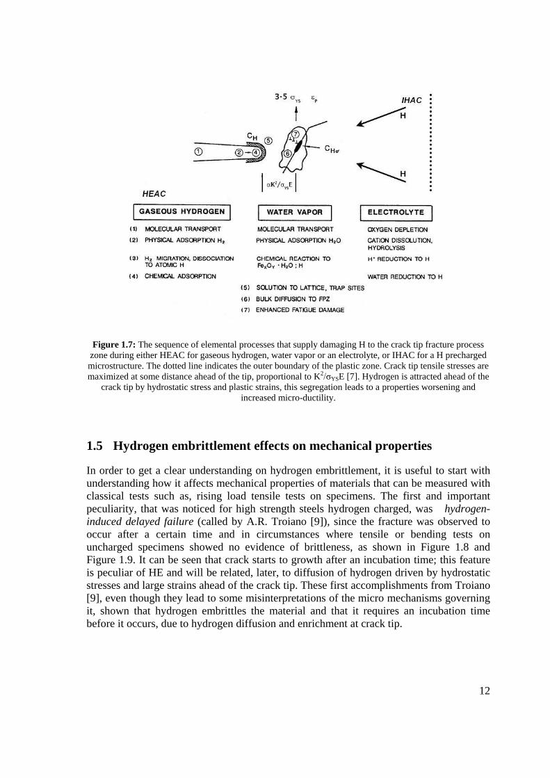
12

Figure 1.7: The sequence of elemental processes that supply damaging H to the crack tip fracture process zone during either HEAC for gaseous hydrogen, water vapor or an electrolyte, or IHAC for a H precharged microstructure. The dotted line indicates the outer boundary of the plastic zone. Crack tip tensile stresses are maximized at some distance ahead of the tip, proportional to K2/σYSE [7]. Hydrogen is attracted ahead of the

crack tip by hydrostatic stress and plastic strains, this segregation leads to a properties worsening and increased micro-ductility.

1.5 Hydrogen embrittlement effects on mechanical properties

In order to get a clear understanding on hydrogen embrittlement, it is useful to start with understanding how it affects mechanical properties of materials that can be measured with classical tests such as, rising load tensile tests on specimens. The first and important peculiarity, that was noticed for high strength steels hydrogen charged, was hydrogen-induced delayed failure (called by A.R. Troiano [9]), since the fracture was observed to occur after a certain time and in circumstances where tensile or bending tests on uncharged specimens showed no evidence of brittleness, as shown in Figure 1.8 and Figure 1.9. It can be seen that crack starts to growth after an incubation time; this feature is peculiar of HE and will be related, later, to diffusion of hydrogen driven by hydrostatic stresses and large strains ahead of the crack tip. These first accomplishments from Troiano [9], even though they lead to some misinterpretations of the micro mechanisms governing it, shown that hydrogen embrittles the material and that it requires an incubation time before it occurs, due to hydrogen diffusion and enrichment at crack tip.

13

Figure 1.8: Typical resistance-time curve for sharply notched specimen (resistance is proportional to crack extension) [8].

Figure 1.9: Schematic representation of delayed failure characteristics of a hydrogenated high strength steel [8].

1.5.1 Effect of hydrogen on ductile-brittle transition temperature DBTT

Hydrogen is supposed to increase DBTT, nevertheless the amount is strictly related to microstructure and hydrogen content. For this reasons it should be assessed every time there is a need to know this variation. This part will be treated and commented largely in

14

paragraph 3.3, since Charpy impact tests have been performed on CV specimens in a wide temperature range for charged and uncharged specimens.

1.5.2 Hydrogen effect on fracture toughness and yielding

There have been many researches and tests to assess hydrogen effect on toughness of steels, especially in pipeline steels. They all show a reduction in toughness but this reduction depends on charging and testing conditions since there are many ways to conduct these tests: hydrogen can be distributed uniformly inside the lattice, it can also be provided by a cathodic reaction at crack surfaces and the amount of hydrogen can vary largely. In Figure 1.10, KIc vs. yield stress for different pipeline steels at room temperature is shown. It can be seen that the reduction is greater for old steels, while for new steel such as X100 there is no variation. In this research [10], CT specimens where charged in an electrolitic solution; the reader is raccomendaed to look to bibiliography for further information. Results on toughness tests will be presented in paragraph 3.4.

Figure 1.10: Fracture toughness of three steels KIi vs. yield stress in air and hydrogen environment [10].

Hydrogen also reduces the ductility of the material that can be assessed through stress-strain behavior. From many investigations, it was observed a drastic reduction on the plastic stress-strain curve strongly dependent on the amount of hydrogen and also on the strain rate (this dependence will be clarified later on). It was shown that hydrogen-charging will enhance the susceptibility of the steel to HIC. The cracks initiate primarily at inclusions, such as aluminum oxides, titanium oxides and ferric carbides, in the steel [11].

15

This macro-behavior will be explained by HELP theory with the hypothesis that hydrogen increases micro-ductility and the macroscopic result is a brittle rupture.

Figure 1.11: Stress-strain curve for X100 under various charging times [11].

1.5.3 Hydrogen effect on fatigue crack propagation

Hydrogen deeply affects the behavior of steels and metals in general, under variable loads below the critical values, since, as already mentioned, hydrogen embrittlement is largely dependent on diffusive phenomena occurring inside the material. In particular, hydrogen drastically increases the crack growth rate up to 40 times [12] and reduces the number of cycles to failure [10], shown respectively in Figure 1.12 and Figure 1.13. Fatigue crack propagation is also sensible to temperature and load frequency as it will be shown in chapter 3. For this reasons, attention has been focused on (da/dN) vs. (ΔK) log-log plot where Paris relation can be pointed out and predicting models can be used.

16

Figure 1.12: Relationship between da/dN and ΔK. Material: SCM435. Hydrogen content indicated by ***→*** means that hydrogen content decreased from *** to *** during fatigue test. ‘‘Frequency switched”

means that the test frequency was switched between f = 2 Hz and f = 0.02 Hz [12].

Figure 1.13: Fatigue endurance curves at initiation and at failures of X52 steel with and without hydrogen charging [10].

17

2 Micromechanics of Hydrogen embrittlement

According to the definition given in paragraph 1.4, in order to analyze and model hydrogen embrittlement, it is necessary to study all the aspects enumerated in paragraph 1.4. For this reason, first, the main concepts of fracture mechanics and stress distribution at crack tip will be reviewed; then, diffusion kinetics and trapping theory will be shown to justify micromechanical models treated in literature such as HEDE, HELD and AIDE.

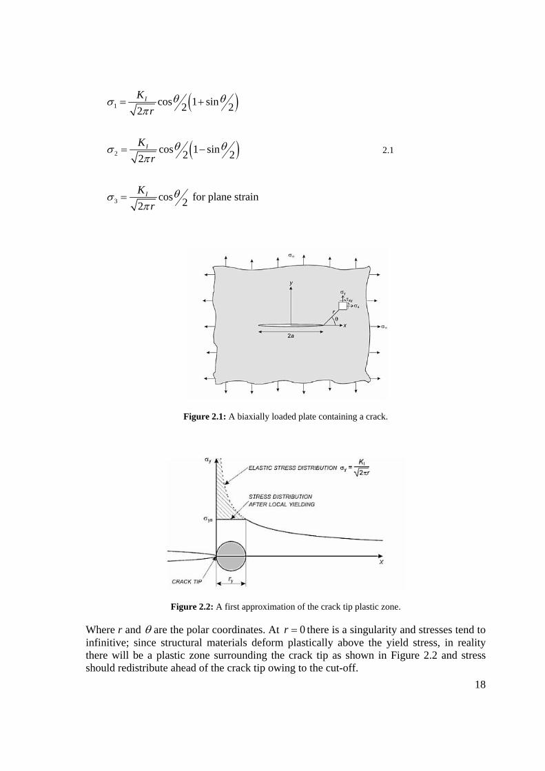
2.1 Fracture mechanics and stress distribution at crack tip

In this paragraph, stress distribution ahead of the crack tip is given. The mathematical derivation, that leads to important relations, will not be given for purpose reasons and the reader is recommended to refer to handbooks on fracture mechanics such as [24] [25] [26], from where many relations have been taken.

For an isotropic material, in the elastic regime, Hooke’s law, that relates stress and strain through Young modulus, can be applied. In linear elastic fracture mechanics, it can be demonstrated that, for the infinite biaxially loaded plate shown in Figure 2.1, the principal stresses, ahead of the crack tip, can be defined through the stress intensity factor KI relative to mode I loading (KI is function of the remote applied stress, crack length and geometry) as it follows:

18

( )

( )

1

2

3

cos 1 sin2 22

cos 1 sin2 22

cos for plane strain22

I

I

I

Kr

Kr

Kr

θ θσπ

θ θσπ

θσπ

= +

= −

=

2.1

Figure 2.1: A biaxially loaded plate containing a crack.

Figure 2.2: A first approximation of the crack tip plastic zone.

Where r and θ are the polar coordinates. At 0r = there is a singularity and stresses tend to infinitive; since structural materials deform plastically above the yield stress, in reality there will be a plastic zone surrounding the crack tip as shown in Figure 2.2 and stress should redistribute ahead of the crack tip owing to the cut-off.

19

Stress state ahead of the crack tip is also very important and it is divided in plane strain and plane stress: plane strain is reached when thickness is 10 times larger than the plastic zone size while plane stress occurs when thickness is comparable to plastic zone. In real case, due to material constrain, there will be a central part of the crack line under plane strain and aside of the specimen an area under plane stress as depicted in Figure 2.3 .

Figure 2.3: Through-thickness plastic zone in a plate of intermediate thickness and relative stress state [25].

The extent of the crack tip plastic zone can vary accordingly if there is a plane strain (large thickness of the specimen) or plane stress (small thickness and high ductility) state. In plane strain, a first approximation is given by Irwin and results equal to:

212 I

yys

Krπ σ

=

2.2

If the material follows Tresca’s yield criterion, and is assumed to be elastic-perfectly-plastic, it is possible to calculate the principal stresses in the plastic zone by imposing the yield criterion; for plane strain it can be demonstrated that [24]:

20

1 2 33 3 2ys ys ysσ σ σ σ σ σ= = = in the plastic zone.

While in the elastic regime stresses are defined by Eq. 2.1., in Elastic-Plastic fracture mechanics stress and strain ahead of the crack tip can be defined by an energetic parameter known as J-integral. From work done independently by Hutchinson and Rice and Rosengren crack tip stresses and strains can be expressed as a function of J assuming a power-law hardening material (HRR model), i.e. the relation between the uniaxial stress and strain is given by the so-called Ramberg-Osgood relation:

0 0 0

nε σ σαε σ σ

= +

2.3

Where n is the strain hardening exponent, α is a dimensionless constant and 0 0 / Eε σ= with 0σ usually equal to the yield stress and 0ε the strain at yielding. For a good prediction of stresses ahead of the tip, it should be evaluated the K dominant zone; if this area is enough large, K is good parameter in describing stresses at the tip. This concept is well depicted in Figure 2.4.

Figure 2.4: stress vs. thickness ahead of the crack tip, the full line indicates the effective stress distribution in the specimen (provino) and in the element (component), the dashed line indicates the stress distribution

according to K. A is the plastic zone and B is the K dominant region [24].

2.2 Diffusion and trapping of hydrogen in iron lattice

As shown before, hydrogen embrittlement is strongly dependent on time. This is a clear evidence that hydrogen embrittlement is a phenomenon governed by kinetics and, hence, by its diffusion and enriching at crack tip.

Atomic hydrogen diffuses easily in metals owing to its small atomic radius (53 pm) that is similar to the length of interstitial sites in metal lattice; hydrogen diffusivity value in iron is around 10-5 cm2/s-1. Hydrogen mobility in carbon steel and low-alloy steel is much

21

higher than any other atoms since its small radius. Parameters that deeply affect hydrogen diffusivity are: Bravais lattice, stress state and plastic deformation [13]. Solubility In Fe-α is equal to 3·10-6 % and 1,6·10-2 % at 900°C while in Fe-γ is slightly higher and equal to 2,3·10-2 % at 900°C. An important remark should be done if considering either FCC or BCC structure. BCC structure, typical of ferrite, can contain (solute) less hydrogen than FCC (typical of austenite); on the other hand, in ferrite, hydrogen diffusion is higher than austenite. In Figure 2.5, hydrogen diffusivity vs. temperature for different lattice structure is plotted; it can be noticed that, in ferrite, diffusivity varies within a large range. Indeed, diffusion is affected by microstructural variables (precipitates and inclusions) and by alloying elements; for further information about this topic it can be referred to [14]. There are other viable mechanisms for hydrogen diffusion that consider dislocations, shortcuts and interstitial jumps. In the next paragraph a simplified model for hydrogen diffusion will be given only considering diffusion coefficient while, in paragraph 2.2.2, hydrogen trapping is considered.

2.2.1 Simplified model for hydrogen diffusion in steel

Hydrogen diffusion in a metal lattice (considered perfectly homogeneous), can be model in a simplified way, with Fick diffusion laws [15]:

J D C= − ∇ 2.4

2C D Ct

∂= ∇

∂ 2.5

Where:

− J [mol·cm-1·s-1] is hydrogen flux; − D [cm2·s-1] is diffusivity; − C [mol·cm-3] is H concentration; − t [s] is time.

First Fick’s law is valid only in stationary conditions when the concentration of the diffusing atoms is constant in time. Otherwise, when concentration is time-dependent Fick’s second law should be used. Diffusivity D can be expressed as a function of temperature through an Arrhenius-like equation:

0 exp AED DR T

= ⋅ − ⋅ 2.6

22

Where:

− D0 [cm2·s-1] is the diffusivity at infinitive temperature; − EA [J·mol-1] is the activation energy for diffusion; − T [K] is the absolute temperature of the diffusion process; − R =8,314472 [J·(mol·K)-1] is the gas constant.

Table 2.1: hydrogen permeation parameters of pearlitic steels measured by gaseous permeation method [16].

Materials Temperature range, °C

Φ0 mol/m⋅s⋅√MPa

HΦ kJ/mol

D0 m2/s

DH kJ/mol

#10 80-330 4,03⋅10-5 35,59 5,07⋅10-8 19,14 #20 80-330 2,59⋅10-5 34,13 3,79⋅10-8 18,57

16Mn 80-330 1,35⋅10-5 33,36 4,2⋅10-8 19,71

Table 2.2: treat condition and composition (wt - %) of steels in research [16].

Materials Treat condition C Mn Si P S Cr Ni Cu

#10 Normalized 0,14 0,50 0,25 - 0,003 0,03 0,03 0,16 #20 Normalized 0,19 0,49 0,23 0,010 0,010 0,01 0,07 0,06

16Mn Hot-rolled 0,13 1,30 0,30 0,028 0,014 - - -

Diffusivity can vary according to other parameters such as concentration of the diffusing atom; this dependence will not be considered in order not to make the analysis heavy.

For a semi-infinite specimen, Eq. 2.5 can be solved by giving suitable boundary conditions:

− 0( 0) .C t const C= = = , bulk concentration of hydrogen

− ( 0) . sC x const C= = = , surface concentration of hydrogen

0

0

14 4s

C C x xerf erfcC C Dt Dt

− = − = −

2.7

23

Where x is the distance from free surface and erf is the error function.

Figure 2.5: Hydrogen diffusivity in ferrite (F), austenite (A) and BCC (G) lattice [14].

2.2.2 Hydrogen trapping in steel

Darken and Smith [17] were apparently the first to suggest that the delayed transport of hydrogen in cold worked steels, as determined by measurements of permeation transients, was caused by attractive interaction between lattice-dissolved hydrogen and microstructural imperfection, or traps. These traps are favorable energy sites where hydrogen places itself either in a reversible or irreversible way, accordingly to the binding energy between hydrogen and the trap. Trap binding energy can vary with temperature, but, in general, when one hydrogen atom moves from an interstitial lattice site to a trap, the probability that it has to move to another site lowers drastically. Since trap-H binding energy is much higher than NILS-H binding energy (NILS = normal interstitial lattice site), the energy barrier to overcome is so high that probability to move out of a trap drops.

24

The more attractive traps, with a high irreversible grade, are inclusions of manganese sulfide (SMn); other possible irreversible trapping sites, ordered with decreasing of irreversibility, are:

oxides and sulfides inclusions titanium, niobium or vanadium carbide and carbonitride cementite.

The consequences of these traps on apparent diffusion of hydrogen are [18]:

increased apparent solubility decreased apparent diffusivity apparent shifting from Fick’s law increased local hydrogen concentration.

Irreversible traps, mentioned above, once saturated, do not take part to any process of hydrogen enriching owing to their high trapping energy, on the other hand, reversible trapping energies are worth to be considered when hydrogen enriching at crack tip needs to be modeled. Reversible trapping sites are: dislocation cores, grain boundaries, interfaces (inclusions and precipitates), vacancies and cavities.

The most important trapping site is given by dislocation cores, since the number of dislocations varies accordingly with the plastic strain ԑp, its number can be very large where stresses are concentrated, such as at crack tip. Many attempts were done in trying to quantify dislocation binding energy. A successful attempt was made by Kumnick and Johnson [19], they calculated trap binding energy for deformed iron and trap density as function of plastic strain. Results of their work are shown in Table 2.3; a binding energy approximately of 60 kJ⋅mol-1 was found for deep trapping state.

Table 2.3: summary of trap parameters of iron determined at different deformation levels and temperatures [19].

% Cold work Trap density NT [m-3]

Binding Energy Eb

0 (Annealed) 8,5⋅1020 ↑

14,3±1,1 kcal⋅mol-1H (59,9±4,6kJ⋅mol-1H)

↓

15 5,9⋅1022 30 5⋅1022 40 7⋅1022 60 1,5⋅1023 80 1,8⋅1023

25

First trapping models were developed separately respectively by: McNabb and Foster [21] and Oriani [20]. Oriani’s theory [20] appears easier to understand and to apply, even if it considers that equilibrium between trapping sites and lattice sites is reached quickly. This assumption can be good if considering slow tests (low strain rate), otherwise it can lead to inaccuracy and time dependence must be considered.

Hydrogen is assumed to reside either at NILS (normal interstitial lattice site) or reversible sites at microstructural defects, such as: internal interfaces or dislocations generated by plastic deformation. The two populations are always in equilibrium according to his theory, such as:

exp1 1

T L B

T L

WRT

θ θθ θ

= − − 2.8

Where:

− Tθ is the occupancy of trapping sites

− Lθ is the occupancy of NILS sites

− WB is the trap binding energy, calculated by Kumnick and Jonhson (Table 2.3) − R is the gas constant and T the absolute temperature

The hydrogen concentration in trapping sites CT, measured in hydrogen atoms per unit volume, can be written as:

T T TC Nθ α= 2.9

Where α denotes the number of sites per trap and TN denotes the trap density in number of traps per unit volume. The hydrogen concentration CL in NILS, measured in hydrogen atoms per unit volume, can be phrased as:

26

L L LC Nθ β= 2.10

Where β denotes the number of NILS per solvent atom, NL denotes the number of solvent atom per unit volume given by NL=NA/VM with NA equal to Avogadro’s number and VM the molar volume of host lattice. Oriani suggested to substitute the diffusivity (Eq. 2.6), valid for a trap free lattice with a new effective diffusion coefficient Deff that takes into account trapping such as:

1

1eff L

T

L

D D NKN

=+

2.11

Where K is the equilibrium constant that can be expressed as exp BWRT

.

2.2.3 Crack tip enriching due to hydrostatic stresses and plastic strain

As mentioned in the previous paragraph, plastic strain can increase the number of dislocations and traps, since from the work of Kumnick and al. ( )T T PN N ε= denotes the trap density in number of traps per unit volume as a function of the amount of local plastic strain Pε (Table 2.3). Another parameter that can affect hydrogen solubility is hydrostatic stress, it was shown that cubic distortion of metal lattice by interstitial H atoms give rise to a macroscopic volume change VH per mol of H; therefore, H atoms interact only with the hydrostatic part of the stress field hσ , changing the chemical potential by a term h HVσ . In thermodynamic equilibrium, the chemical potential of H has to be the same in all the regions on the sample. Thus an inhomogeneous spatial distribution of hydrostatic stresses (such as at crack tip), leads to a redistribution of H-concentration according to [22] :

00

0

0

( 0) ln ( 0)

ln ( )

( ) ( ) exp

H h H H h

H h H

h H

RT c

RT c x V

x Vor c x cRT

µ σ µ µ σ

µ σ

σ

= = + = ≠

= + +

=

2.12

27

Where 0Hµ is the standard value of Hµ and 0c is the H-concentration at zero hydrostatic

stress (e.g. far away from hydrostatic stresses). Eq. 2.12 is valid for low concentrations only, i.e. for the ideal dilute case [22]. Eq. 2.12 can be rearranged and written as it follows:

01

0 exp1 1 3

L L H

L L

J VRT

θ θθ θ

= − − 2.13

Where J1 is the first stress invariant of the stress tensor and is divided by 3 to give the hydrostatic stress and 0

Lθ is the NILS occupancy when no stress is applied.

2.2.4 Modified hydrogen diffusion model

At crack tip stresses and strain cannot be neglected and they must be taken into account in a time-dependent diffusion model, McNabb and Foster proposed the following equation, derived from a modification of Fick’s law, as the governing equation for transient hydrogen diffusion accounting for trapping and hydrostatic drift [21]:

( )L TT L L

C N D Ct t

θ∂ ∂+ = ∇ ∇

∂ ∂ 2.14

Working out Eq. 2.14 with Eq. from 2.8 to 2.13 leads to the governing equation for hydrogen diffusion [23]:

, ,,

03

L T P HT L ii L kk i

ieff P

dC dN d DVD DC CD dt d dt RT

εαθ σε

+ − + =

2.15

28

In this equation ,( ) ( ) /i ix= ∂ ∂ , the derivative of the argument respect to the spatial coordinate ijσ is the Cauchy stress. Equation 2.15 shows that in order to calculate the hydrogen distribution within a solid, one should solved a coupled problem of hydrogen diffusion and elastoplasticity. Oriani’s model assumes that the trap filling kinetics is very quick. Consequently, the effective diffusion coefficient Deff is less than the normal NILS diffusion coefficient D as long as traps are not saturated or as new traps are created by plastic straining [23].

2.3 Micromechanical theories of HE

Before it was shown that stresses distribution and plastic strain can largely modify hydrogen concentration and diffusion and, since at crack tip these conditions occur, recent theories have been introduced to link the high local H concentration to damaging micro-mechanisms that lead to failure. The first theory, called hydrogen enhanced decohesion and introduced by Troiano, was later taken on by other theories involving dislocation models (HELP and AIDE). It is still impossible to assess which is the most correct theory, nevertheless, it was shown that all three can compete to hydrogen embrittlement and the prevailing should be assessed case by case. In this paragraph all three theories will be shown with relative modeling. In his review of hydrogen assisted cracking, Gangloff [7] gives a clear overview on the main theories up to date on internal HE that will be reported below; nevertheless, his work is mainly qualitative and, for this reason, quantitative models will be added from literature.

2.3.1 HEDE, hydrogen enhanced decohesion

The HEDE mechanism was first suggested by Troiano, and developed in detail by Oriani and coworkers. In this model, H segregates at the crack tip FPZ (fracture process zone) and, there, reduces the cohesive bonding strength between metal atoms. The HEDE gives the concept that H damage occurs in the FPZ when the local crack tip tensile stress exceeds the maximum-local atomic cohesion strength, reduced by the presence of H. In the HEDE scenario, H damage sites are located at a distance ahead of the crack tip surface where tensile stresses are maximized. Predictions are derived from knowledge of crack tip stress, H concentration at damage sites, and its relationship with the interatomic bonding force vs. atom displacement. A consensus is emerging that HEDE is the dominant mechanism for IHAC (internal hydrogen assisted cracking) and HEAC (hydrogen environmentally assisted cracking) in high strength alloys that do not form hydrides. HEDE is likely for several reasons. First, large concentrations of H should accumulate ahead of the crack owing to very high crack tip stresses, in addiction H trapping along a crack path [7].

Dislocations promote a local stress concentration around decohesion sites so to weaken the metal bonds. Decohesion can take place in different zones such as: at crack tip, or right

29

ahead, or where dislocations increase stress concentration. Fractographs have shown that this mechanism occurs especially with brittle fracture surfaces; typical fracture surfaces caused by HEDE are intergranular and transgranular and are usually smooth, although also plasticization can be observed [28].

Oriani and Josephic [27] have shown that over a wide range of hydrogen concentrations the tensile stress required to fracture a high strength steel may be approximated by:

0( )F C F Cα= − 2.16

Where 0F is the fracture tensile stress with no hydrogen, α is a constant of the material that can be experimentally extrapolated and ( )F C is the cohesive force between the metal atoms in the lattice, function of H concentration.

Concluding, all HEDE-based models of macroscopic KTH and da/dt properties contain one or more adjustable parameters owing to uncertain features of the crack tip problem.

Figure 2.6: HEDE mechanism representation, iron bonds are weaken by hydrogen in the lattice, dislocation can increase stress field [28].

2.3.2 Hydrogen Affected Localized Plasticity, HELP and AIDE

It was suggested that H stimulates dislocation mechanics that localize plastic deformation enough, resulting in subcritical crack growth with brittle characteristics on the macroscopic scale. Two variations of this concept have been advanced as the AIDE and HELP mechanisms.

30

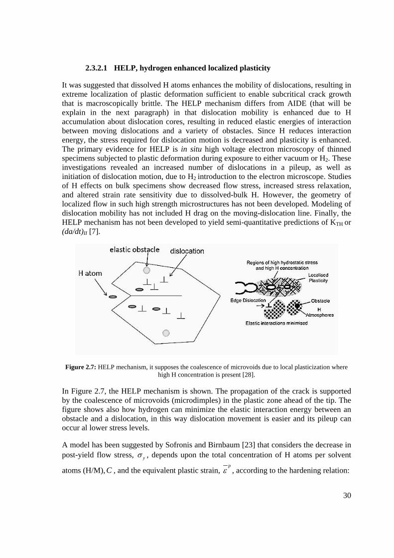
2.3.2.1 HELP, hydrogen enhanced localized plasticity

It was suggested that dissolved H atoms enhances the mobility of dislocations, resulting in extreme localization of plastic deformation sufficient to enable subcritical crack growth that is macroscopically brittle. The HELP mechanism differs from AIDE (that will be explain in the next paragraph) in that dislocation mobility is enhanced due to H accumulation about dislocation cores, resulting in reduced elastic energies of interaction between moving dislocations and a variety of obstacles. Since H reduces interaction energy, the stress required for dislocation motion is decreased and plasticity is enhanced. The primary evidence for HELP is in situ high voltage electron microscopy of thinned specimens subjected to plastic deformation during exposure to either vacuum or H2. These investigations revealed an increased number of dislocations in a pileup, as well as initiation of dislocation motion, due to H2 introduction to the electron microscope. Studies of H effects on bulk specimens show decreased flow stress, increased stress relaxation, and altered strain rate sensitivity due to dissolved-bulk H. However, the geometry of localized flow in such high strength microstructures has not been developed. Modeling of dislocation mobility has not included H drag on the moving-dislocation line. Finally, the HELP mechanism has not been developed to yield semi-quantitative predictions of KTH or (da/dt)II [7].

Figure 2.7: HELP mechanism, it supposes the coalescence of microvoids due to local plasticization where high H concentration is present [28].

In Figure 2.7, the HELP mechanism is shown. The propagation of the crack is supported by the coalescence of microvoids (microdimples) in the plastic zone ahead of the tip. The figure shows also how hydrogen can minimize the elastic interaction energy between an obstacle and a dislocation, in this way dislocation movement is easier and its pileup can occur al lower stress levels.

A model has been suggested by Sofronis and Birnbaum [23] that considers the decrease in post-yield flow stress, yσ , depends upon the total concentration of H atoms per solvent

atoms (H/M), C , and the equivalent plastic strain, p

ε , according to the hardening relation:

31

00

( , ) ( ) 1p

p

y C C εσ ε σε

= +

2.17

Material softening follows an assumed relationship:

( )0 0( ) 1 1C Cσ ξ σ = − + 2.18

Where ξ denotes a material softening parameter (≤ 1, measured on ductile void growth) that describe the intensity of hydrogen-induced softening, and 0σ defines the initial yield stress in absence of hydrogen [29].

2.3.2.2 AIDE, adsorption induced dislocation emission

Figure 2.8: AIDE mechanism: (a) when crack is propagating transgranularly, the alternate yield promotes the coalescence of the crack with microvoids in the plastically deformed zone right ahead of the crack; (b)

when crack is propagating with a brittle mechanism [28].

Lynch [28] argued that H-induced weakening of metal-atom bond strength results in enhanced emission of dislocations from crack tip surfaces where H is absorbed. AIDE attributes H-enhanced crack growth as predominantly due to this focused emission of dislocations, exactly from the crack front and along intersecting planes that geometrically favor sharp-crack opening and advance rather than crack tip blunting in the absence of H. During loading, plastic deformation is also triggered within the crack tip plastic zone; and microvoids formation, with or without an assist from dissolved H, could occur. The link-up of voids adds a component to crack advance and maintains a sharp crack tip by interacting with the intense slip bands from crack tip dislocation emission. The crack

32

surface should reflect this advance process and contain facet-like features parallel to the plane that bisects crack tip slip planes, as well as a high density of microvoids if this latter feature occurs. Voids should occur on a size scale that is substantially less than those formed about inclusions and larger dispersoids or precipitate particles during fracture without H and AIDE. Facets may be parallel to low index planes for certain symmetric slip plane configurations, but also along higher index planes if the crack tip slip state is unbalanced. Intergranular cracking in the AIDE formulation reflects preferential adsorption of H along the line of intersection between the grain boundary plane and crack front, and perhaps a higher density of precipitates that may form preferentially along grain boundaries. This mechanism is best suited for HEAC; however, H localization to a crack tip during IHAC could also be result in AIDE. The AIDE mechanism is debated because of weaknesses in the supporting evidence. The structure of slip about a crack tip in a hydrogen exposed metal has never been characterized sufficiently to show H stimulated dislocation emission and associated geometric crack extension [7]. In Figure 2.8 two different mechanisms for crack growth owing to AIDE mechanism are shown, the above mentioned features can be found. For this model there are not reliable quantitative relations; in many researches, investigations have been conduction in a short lapse of time and within few atomic planes so that it is very tough to connect to the macro behavior.

33

3 Experimental procedures and results

Tests have been performed on F22 and X65 steels which will be described in this chapter.

An innovative electrochemical non-hazardous hydrogen charging technique has been developed at Dipartimento di Chimica, Materiali e Ingegneria Chimica “G. Natta”. Thanks to this technique, it has been possible to control the amount of hydrogen present in the metal lattice ( around 0,9-1,3 ppm) and hence to perform mechanical tests on H-charged material, description of the technique will not be given in this work, nevertheless for an accurate description the reader may refer to [30].

3.1 Materials characterization

The two steels, which have been investigated in this research, are widely used in piping for oil transportation and are named as it follows:

A 182 F22 (ASTM or ASME denomination) [31] API 5L X65 (API denomination) [36].

3.1.1 A182F22 steel

The first steel, also known with the commercial name A182 F22, according to ASME regulation [31], is forged steel. This steel is designed for high temperature and high pressure working conditions. Its good mechanical properties rely on a fine dispersion of

34

molybdenum carbides and a small amount of chromium that increases corrosion properties. According to regulation its mechanical properties are guaranteed until 600 °C.

The chemical composition in weight percentage of F22 (also known as 2 ¼ Cr-1Mo) is shown in Table 3.1.

Table 3.1: Chemical composition [wt%] of F22.

C Mn S P Si Cr Mo 0,05 – 0,15 0,3 – 0,6 0,025 0,025 0,5 2,0–2,5 0,87 – 1,13

This steel according to ISO regulation is named 10 Cr-Mo 9-10. In Table 3.2 mechanical and physical properties from literature are reported [31].

Table 3.2: Material properties of F22 steel.

Properties Temperature [K] Value E [MPa] 293,15 206539

153,15 219942,8 Ry [MPa] 293,15 468

Ruts [MPa] 293,15 592 ν 293,15 0,288

cp [kJ/kg K] 293,15 0,442 153,15 0,27625

α [mm/mm K] 293,15 1,11·10-5 153,15 9,54·10-6

k [W/m K] 293,15 36,3 153,15 28,5

ρ [kg/m3] 293,15 7860

All specimens that have been used in mechanical tests were made from the pipe bulk, provided by Ring Mill; the steel was first forged, then hot worked and finally quenched. Pipe dimensions are reported below:

Outer diameter: 0 320 D mm=

Thickness: 65 t mm=

In Table 3.3 the chemical composition experimentally observed is shown and in Table 3.4 hardness profile along thickness direction is reported. It was observed a good homogeneity of hardness along the whole thickness. F22 microstructure along thickness is shown in figure 2.1. All these measurements were carried out at Centro sviluppo materiali (CSM).

35

Table 3.3: chemical composition experimentally observed.

Chemical element

C Mn Cr Mo Ni Nb V Ti F22 0.14 0.43 2.25 1.04 0.08 0.023 <0.01 <0.01

Table 3.4: Hardness values along thickness for F22.

F22 - HV 10 Average OD 193 192 192 192 MW 195 192 187 193 ID 190 187 187 188

36

Figure 3.1: F22 microstructure along thickness.

Microstructure is homogeneously distributed along thickness and formed by martensite and bainite. Specimens for testing were made out the pipe as depicted in Figure 3.2, where it can be seen: tensile specimens [32], CV specimen [33] and CT specimens [34].

Three tensile tests have been carried out to obtain static properties of the material according to regulation [32]. Average test results are shown in Table 3.5.

Table 3.5: mechanical properties of F22 steel.

Mechanical Properties Value Dispersion Yield strength Ry [MPa] 468 2.7

Ultimate tensile strength Ruts [MPa] 592 2.1 Young Modulus E [MPa] 206500 1500

Elongation E [%] 20 2.5

37

Figure 3.2: Specimens designing for tests.

As it can be noticed, material properties are typical of ductile steel, dispersion of results is well-centered. The characteristic stress-strain curve for F22 is shown in Figure 3.3. All tests results and curves are very similar, for this reason it’s worth nothing to show them.

38

Figure 3.3: Stress-strain characteristic curve for F22.

3.1.2 API 5L X65 steel

The second steel is commercially named API 5L X65. Its regulation is API [36] (American petroleum institute) that is translated with few differences in ISO [35]. This steel is mainly used in piping for petroleum and natural gas transportation. Pipes are produced according to two different techniques: seamless and welded; in our case pipes are seamless. The chemical composition of X65 in weigh percentage is shown in Table 3.6 [31].

Table 3.6: Chemical composition of X65 steel.

C Mn P S V Nb Ti 0,28 1,4 0,03 0,03 Sum < 0,15

X65 is a low alloy steel with 1,4 % of manganese that increases toughness and quenching properties. In Table 3.7 mechanical and physical properties of X65 are reported.

0

100

200

300

400

500

600

700

0 0,02 0,04 0,06 0,08 0,1 0,12 0,14

Stre

ss [M

Pa]

Strain [mm/mm]

39

Table 3.7: Mechanical and physical properties of X65 steel.

Properties Temperature [K] Value E [MPa] 293,15 201966

153,15 212196 Ry [MPa] 293,15 504

Ruts [MPa] 293,15 603 ν 293,15 0,301

cp [kJ/kg K] 293,15 0,489 153,15 0,2843

α [mm/mm K] 293,15 1,05·10-5 153,15 9,38·10-6

k [W/m K] 293,15 35,8 153,15 28,1

ρ [kg/m3] 293,15 7860

All specimen were made directly from the seamless pipe provided by “Tenaris S.A.” company, its dimensions are:

Outer diameter: 0 323 D mm=

Thickness: 46 t mm=

Specimens were made out of the pipe according to the Figure 3.2, pipe’s outer diameter is equal to 323 mm and thickness 46 mm. The chemical composition, experimentally observed, is reported in Table 3.8. In

Table 3.9 hardness profile along thickness is shown.

Table 3.8: Chemical composition experimentally observed [Wt%] for X65.

X65 Chemical Element

C Mn Cr Mo Ni Nb V Ti 0.11 1.18 0.17 0.15 0.42 0.023 0.06 <0.01

Table 3.9: Hardness profile along thickness for X65.

X65 - HV 10 Average OD 243 OD 243 OD MW 195 MW 195 MW ID 220 ID 220 ID

40

Hardness profile is less homogeneous than F22; hardness is higher near the outer diameter and smaller close to the inner diameter. X65 microstructure along thickness is shown in figure 2.4.

Figure 3.4: Microstructure of X65.

41

Near the center of the pipe, acicular ferrite can be noticed, X65 has a less well-distributed microstructure along thickness, nevertheless distribution is well acceptable; ferrite structure is non equiassic and it was formed during a continuous cooling process at temperature slightly above upper bainite and also bainite is present near the outer diameter.

X65 steel microstructure is equiassic and acicular ferrite with finely dispersed carbides. The microstructure is rather homogeneous, no differences are visible among different alignments (internal, center, external) or different orientations (longitudinal, transversal). Inclusion shape is round as expected for a “sour gas” material treated with calcium in order to have only spheroidized inclusions (type D globular inclusions) and no elongated inclusions are present; longitudinal and transverse orientation don’t show any difference neither as density nor as mean diameter (1.5 μm long. surface, 1.4 μm transv. surface); no central segregation is present; inclusion density is high: on the external surface slightly lower and with larger dimension (mean diameter 1.7 μm and maximum diameter up to 7-8 μm).

Five tensile tests have been performed at room temperature to obtain static properties of the material according to regulation [32]. Average test results are reported in Table 3.10.

Table 3.10: Mechanical properties experimentally observed for X65.

Mechanical properties Value Dispersion Yield strength Ry [MPa] 511 6.7

Ultimate tensile strength Ruts [MPa] 609 5.7 Young Modulus E [MPa] 206208 6049

Elongation E [%] 21 6.5

It was observed that mechanical properties of X65 are those typical of ductile steels, results dispersion is well concentrated; compared to F22, X65 shows a higher, though still good, results dispersion.

Stress-strain curve from one of the tensile tests is depicted in Figure 3.5. All other stress-strain curves are similar to this one and it’s worth nothing to show them.

42

Figure 3.5: Stress-strain curve for X65 steel.

3.2 Cooling and transportation technique

As mentioned, tests needed to be performed among a large number of specimens varying temperature and in particular at very low temperatures.

Specimens were first hydrogen charged at “Politecnico di Milano” laboratories in the department of Chemical Engineering, Chemistry and Materials “G. Natta”. Hydrogen content in the specimens was measured by reference specimens [30] and equal to a value in the range of 0,9-1,3 ppm.

After the charging process, specimens were transported by keeping the specimens in a liquid nitrogen thermostatic bath during the transportation at -196°C.

In order to carry out tests at low temperatures two different cooling techniques have been used:

MTS 651 environmental chamber Ethanol – liquid nitrogen thermostatic bath.

Test procedures, settings, analysis, controls and instruments were chosen accordingly to ISO [37]. A large number of tests were carried out varying temperature, by placing the specimens either in the environmental chamber or in the thermostatic bath for 30 minutes

0

100

200

300

400

500

600

700

0 0,02 0,04 0,06 0,08 0,1 0,12 0,14 0,16

Stre

ss [M

Pa]

Strain [mm/mm]

43

at constant temperature; subsequently tests were performed in a lapse of time shorter than 5 seconds between extraction operation and test. In addition, as stated in the regulation, pliers to handle the specimens were kept at the testing temperature.

3.2.1 Environmental Chamber

The environmental chamber, shown in Figure 3.6 uses liquid nitrogen to set its temperature until T = -128°C. Nitrogen stored inside the vessel vaporizes when it reaches the chamber. Outside the chamber there is a control unit able to adjust the amount of nitrogen flowing inside the chamber and then able to keep a stable temperature inside, temperature then can be manually set.

Temperature inside the chamber is measured by a thermocouple placed in the bottom of the chamber, close to the gas flow-in grid. Environmental chamber was used for toughness tests (J-integral) and for fatigue crack growth tests since the specimen was exposed to atmosphere for a lapse of time too long. In Figure 3.6, it is also shown the testing machine, MTS 810, used for crack growth and toughness test.

Figure 3.6: Image of the environmental chamber and the nitrogen vessel.

3.2.2 Ethanol-liquid nitrogen conditioning bath

In order to bring the specimens at the testing temperature, a quick and effective method was used: it consists in immersing the specimens in an ethanol-liquid nitrogen bath kept at the requested temperature by adjusting the correct proportion between ethanol and liquid nitrogen. The equipment includes a small insulated plastic vessel with a void zone between the inner and outer surfaces and a lid on top as show in Figure 3.7.

44

Figure 3.7: Image of the insulated vessel for Charpy specimens cooling whose temperature is controlled by a thermocouple.

A thermocouple, bound to a weight was placed inside the vessel to control the bath temperature. Inside the vessel, ethanol and liquid nitrogen, collected directly from the tank, were drawn (nitrogen vaporizes while absorbing heat from ethanol). This mixture can reach temperatures close to -110 °C, indeed -114 °C is the ethanol solidification temperature. Then by controlling the amount of nitrogen poured inside the vessel it is possible to control the bath temperature.

Figure 3.8: Ethanol-liquid nitrogen bath inside the thermal vessel.

It was quite complicated to reach temperatures close to -110°C because ethanol tends to solidify, going towards a jelly state; only through a careful stirring it was possible to keep the bath in a liquid state. Once the correct temperature of the bath was reached it was possible to immerse the specimens inside. In case of a liquid environment, the regulation

45

suggests to keep the specimen for at least 5 minutes inside. When the cover is closed the temperature inside the vessel is maintained constants and the thermocouple enables to check the temperature. Charpy specimens are one bulk piece with no holes and quite thin, for this reason it is not possible to monitor the temperature inside them; nevertheless it is reasonable to say that thanks to the long immersing time the correct temperature is reached throughout the whole specimen. This bath was used for all three tests; indeed, for Charpy impact energy, it was sufficient to bring specimen at the requested temperature while for other tests (crack growth and toughness) it was used to bring the specimen at the test temperature faster than keeping it inside the environmental chamber.

3.3 Charpy impact test

Charpy impact tests were performed on CV specimens shown in Figure 3.2 varying hydrogen content (yes/no) and the position inside the pipe thickness were they have been extracted and according to regulation [33]. For impact tests, it was used a Charpy pendulum as shown in Figure 3.9, pendulum was calibrated before testing.

Figure 3.9: Charpy pendulum for Impact tests presents at Falco laboratories (Politecnico di Milano).

3.3.1 Charpy impact test of F22 steel

In Figure 3.10 the Charpy impact energy values as a function of temperature for F22 steel are depicted.

46

Ductile-brittle transition temperature (DBTT) is defined accordingly to regulation [37] as the temperature with a Charpy toughness equal to 27[J]. It comes out clearly that for the specimens who were hydrogen charged DBTT is much higher than the one for uncharged specimens. In Figure 3.11 the percentage of brittle area as a function of temperature is depicted.

Figure 3.10: Resilience as a function of temperature for F22 steel.

0

25

50

75

100

125

150

175

200

225

250

275

300

-140 -130 -120 -110 -100 -90 -80 -70 -60 -50 -40 -30 -20 -10 0 10 20 30 40

Ener

gy [J

]

Temperature [°C]

Non-HydrogenatedHydrogenated

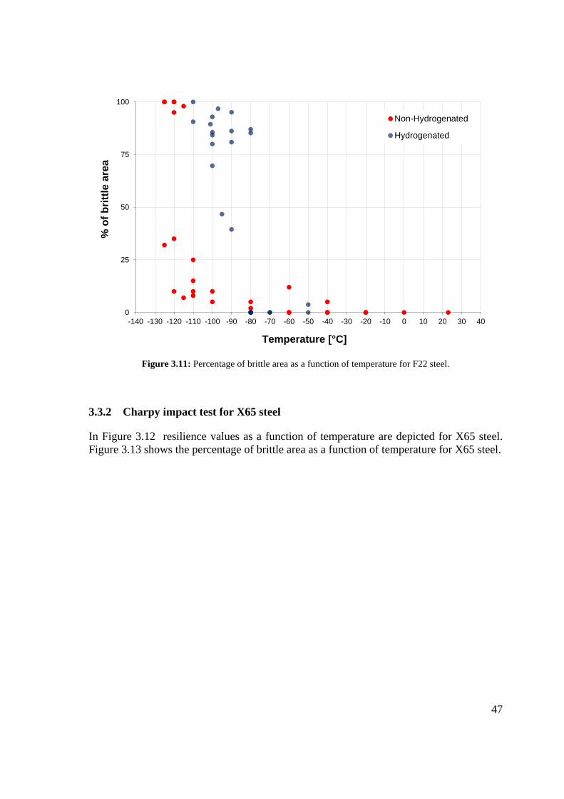
47

Figure 3.11: Percentage of brittle area as a function of temperature for F22 steel.

3.3.2 Charpy impact test for X65 steel

In Figure 3.12 resilience values as a function of temperature are depicted for X65 steel. Figure 3.13 shows the percentage of brittle area as a function of temperature for X65 steel.

0

25

50

75

100

-140 -130 -120 -110 -100 -90 -80 -70 -60 -50 -40 -30 -20 -10 0 10 20 30 40

% o

f brit

tle a

rea

Temperature [°C]

Non-Hydrogenated

Hydrogenated

48

Figure 3.12: Charpy toughness values as function of temperature for X65 steel.

Figure 3.13: Percentage of brittle area as a function of temperature for X65 steel.

0

25

50

75

100

125

150

175

200

225

250

275

-110 -100 -90 -80 -70 -60 -50 -40 -30 -20 -10 0 10 20 30

Ener

gy [J

]

Temperature [°C]

Non-Hydrogenated

Hydrogenated

0

25

50

75

100

-110 -100 -90 -80 -70 -60 -50 -40 -30 -20 -10 0 10 20 30

% o

f brit

tle a

rea

Temperature [°C]

Non-Hydrogenated

Hydrogenated

49

3.3.3 Remarks on results

It was observed a remarkably different behavior between X65 and F22 steels whether hydrogen charged or uncharged. In particular the uncharged F22 steel does not show any change in energy to rupture until a temperature equal to -100°C: energy, lost during the test whether at -100°C or room temperature, is almost the same. This is supported by the percentage of brittle area: on the specimens, tested at T = -100°C, percentage of brittle is between 5 % - 10 %. K-T curve starts to drop slightly around T = -110°C; while for lower temperatures, around -120 °C, ductile-brittle transition occurs.

Tests on H-charged F22 steel show Charpy impact energies smaller than the one of hydrogen free. As it can be seen from plots in Figure 3.10 and Figure 3.11 , at temperatures around -90°C fragile behavior occurs. Moreover, it was observed the difference in the transition temperature: it appears clearer for hydrogen free specimens while for charged specimens the transition is “blurred”. Low values of Charpy toughness for F22 steel appear also at temperature equal to - 80°C.

For F22 it was found a difference in transition temperatures for charged and uncharged specimens of about 30°C and an increase of the transition temperature from -120°C to -90°C.

For X65 specimens the transition is less clear: it was observed indeed a broad area between -60°C and -100°C, in which a clear ductile-brittle transition cannot be spotted. With respect of ISO standards for the determination of the ductile-brittle transition temperature (when energy absorption in the impact is equal to 27 J), it is still possible to find the transition temperature and in this case was found equal to a value around -100°C.

X65 uncharged specimens does not show any big difference, even if a remarkable number of specimens shows a fragile transition around T = - 90°C.

It was assumed that hydrogen embrittlement effect, on X65 for high impact rate, is smaller than F22 steel. Results data can be found in Appendix A.1.

3.4 Toughness Tests

3.4.1 Test methodology

Toughness tests have been carried out at Mechanics Department laboratories in Politecnico di Milano. Test methodology is governed by the regulation [34] modified with side grove according to [39]. Materials tested in this research present a strong ductile behavior and for this reason, it turned out to be very difficult to evaluate KIC, accordingly to the international regulation that imposes large thickness of the specimens. Therefore it

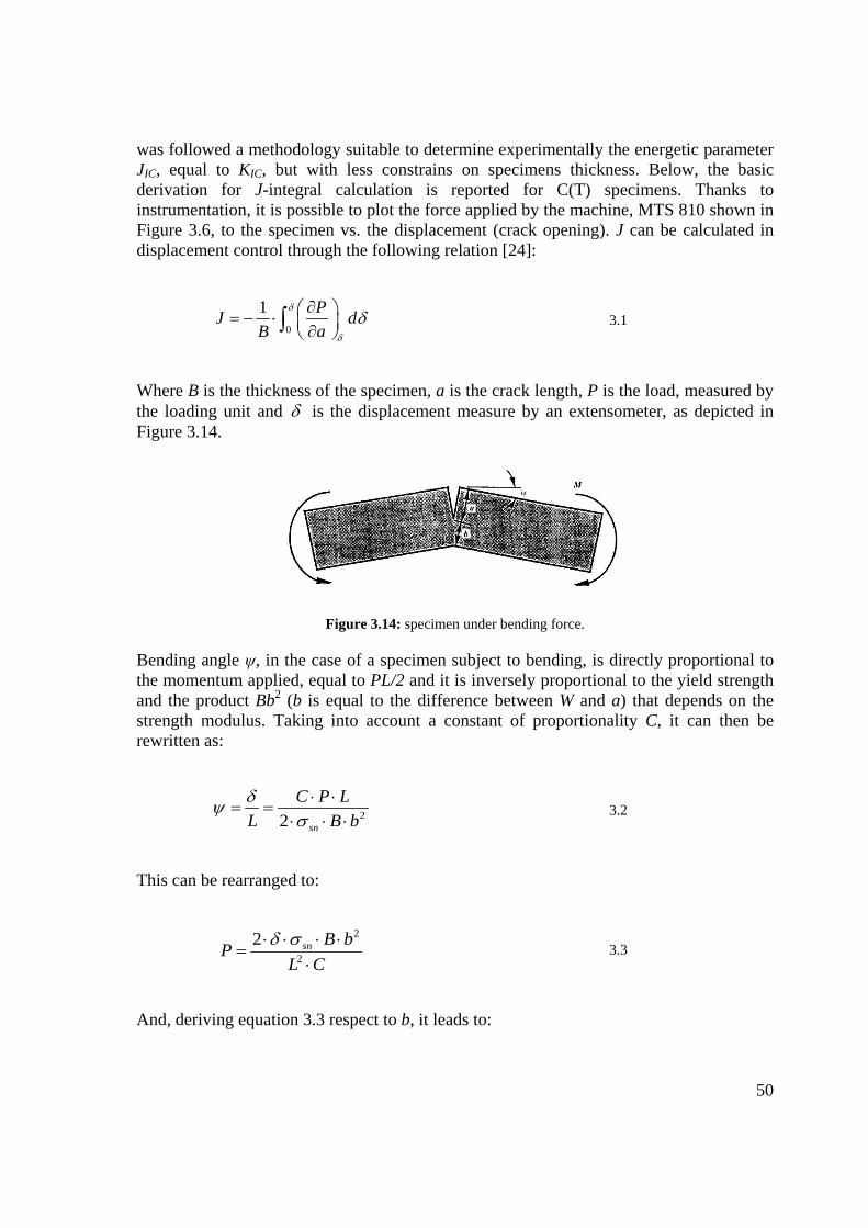
50

was followed a methodology suitable to determine experimentally the energetic parameter JIC, equal to KIC, but with less constrains on specimens thickness. Below, the basic derivation for J-integral calculation is reported for C(T) specimens. Thanks to instrumentation, it is possible to plot the force applied by the machine, MTS 810 shown in Figure 3.6, to the specimen vs. the displacement (crack opening). J can be calculated in displacement control through the following relation [24]:

0

1 PJ dB a

δ

δ

δ∂ = − ⋅ ∂ ∫ 3.1

Where B is the thickness of the specimen, a is the crack length, P is the load, measured by the loading unit and δ is the displacement measure by an extensometer, as depicted in Figure 3.14.

Figure 3.14: specimen under bending force.

Bending angle ψ, in the case of a specimen subject to bending, is directly proportional to the momentum applied, equal to PL/2 and it is inversely proportional to the yield strength and the product Bb2 (b is equal to the difference between W and a) that depends on the strength modulus. Taking into account a constant of proportionality C, it can then be rewritten as:

22 sn

C P LL B bδψ

σ⋅ ⋅

= =⋅ ⋅ ⋅

3.2

This can be rearranged to:

2

2

2 sn B bPL C

δ σ⋅ ⋅ ⋅ ⋅=

⋅ 3.3

And, deriving equation 3.3 respect to b, it leads to:

51

2

4 2sn B bP Pb L C b

δ σ⋅ ⋅ ⋅ ⋅∂ ⋅= =

∂ ⋅ 3.4

Since da db= − it can be written as:

P Pa b

∂ ∂= −

∂ ∂ 3.5

Then:

2P Pa b

∂= −

∂ 3.6

It can be rewritten as:

0 0

1 2 2PJ d P dB b Bb

δ δδ δ⋅

= ⋅ = ⋅ ⋅∫ ∫ 3.7

It can be noticed that the integral of the Eq. 3.7 is equal to the area under the plot P-δ in Figure 3.15:

Figure 3.15: P-δ plot registered during the test of J integral.

In this case, when specimen C(T) is subject to an aperture according to mode I, the final relation is modified by taking into account the different stress state in the specimen C(T) compared to the one under bending force.

The relation then becomes:

52

0J P d

B bδη δ= ⋅ ⋅

⋅ ∫ 3.8

Where η depends on the ratio a/W and it is slightly higher than 2.

In order to calculate the value of J, tests have been carried out according to ASTM [34] and [38] through the compliance method. This method enables to save time and specimens for the calculation of the requested value, because it is possible to plot the whole curve J-Δa with just one specimen.

The compliance method is based on the measurement of the compliance C, as indicated in Figure 3.16; it consists in loading the specimen increasing P, then removing partially the load, measure the compliance and repeat it for every loading ramp.

Figure 3.16: Load as a function of displacement during a toughness test: to be noted the decrease of the slope (opposite of compliance) while increasing the displacement.

This process goes on until the last load and/or rupture of the specimen (that could not occur for very tough materials such those one). Figure 3.17 shows a plot of a toughness test.

53

Figure 3.17: Plot of a toughness test showing the load versus the displacement measured by a clip on gage.

The slope of the loading ramps gives the value of the compliance. Through calibration it is possible to obtain the value of the crack length a during the test and the Δa increases. The intersection between the characteristic curve of the material with the blunting line (characteristic line indicated by regulation to obtain JIC) gives the value of JIC. The blunting line can be calculated through this equation (according to regulation [34]):

2 ysJ aσ= ⋅ ⋅∆ 3.9

Where ysσ is the yield strength. Specimens used in this research are Compact Tension specimens as shown in Figure 3.2. This enables to contain the amount of material needed and to have more compact and easy to handle specimen that has to undergo to different operation such as: hydrogen charging and mechanical testing. Geometry of the specimen is show in Figure 3.18.

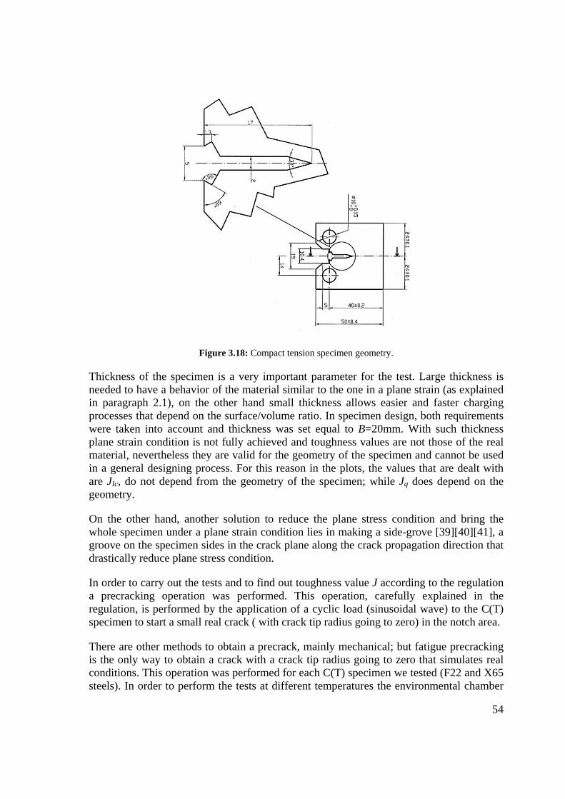
54

Figure 3.18: Compact tension specimen geometry.

Thickness of the specimen is a very important parameter for the test. Large thickness is needed to have a behavior of the material similar to the one in a plane strain (as explained in paragraph 2.1), on the other hand small thickness allows easier and faster charging processes that depend on the surface/volume ratio. In specimen design, both requirements were taken into account and thickness was set equal to B=20mm. With such thickness plane strain condition is not fully achieved and toughness values are not those of the real material, nevertheless they are valid for the geometry of the specimen and cannot be used in a general designing process. For this reason in the plots, the values that are dealt with are JIc, do not depend from the geometry of the specimen; while Jq does depend on the geometry.

On the other hand, another solution to reduce the plane stress condition and bring the whole specimen under a plane strain condition lies in making a side-grove [39][40][41], a groove on the specimen sides in the crack plane along the crack propagation direction that drastically reduce plane stress condition.

In order to carry out the tests and to find out toughness value J according to the regulation a precracking operation was performed. This operation, carefully explained in the regulation, is performed by the application of a cyclic load (sinusoidal wave) to the C(T) specimen to start a small real crack ( with crack tip radius going to zero) in the notch area.

There are other methods to obtain a precrack, mainly mechanical; but fatigue precracking is the only way to obtain a crack with a crack tip radius going to zero that simulates real conditions. This operation was performed for each C(T) specimen we tested (F22 and X65 steels). In order to perform the tests at different temperatures the environmental chamber

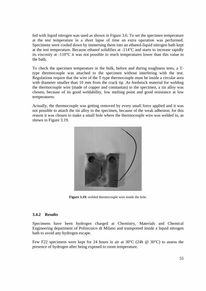
55

fed with liquid nitrogen was used as shown in Figure 3.6. To set the specimen temperature at the test temperature in a short lapse of time an extra operation was performed. Specimens were cooled down by immersing them into an ethanol-liquid nitrogen bath kept at the test temperature. Because ethanol solidifies at -114°C and starts to increase rapidly its viscosity at -110°C it was not possible to reach temperatures lower than this value in the bath.

To check the specimen temperature in the bulk, before and during toughness tests, a T-type thermocouple was attached to the specimen without interfering with the test. Regulations require that the wire of the T-type thermocouple must be inside a circular area with diameter smaller than 10 mm from the crack tip .As feedstock material for welding the thermocouple wire (made of copper and constantan) to the specimen, a tin alloy was chosen, because of its good weldability, low melting point and good resistance at low temperatures.

Actually, the thermocouple was getting removed by every small force applied and it was not possible to attach the tin alloy to the specimen, because of the weak adhesion; for this reason it was chosen to make a small hole where the thermocouple wire was welded in, as shown in Figure 3.19.

Figure 3.19: welded thermocouple wire inside the hole.

3.4.2 Results

Specimens have been hydrogen charged at Chemistry, Materials and Chemical Engineering department of Politecnico di Milano and transported inside a liquid nitrogen bath to avoid any hydrogen escape.

Few F22 specimens were kept for 24 hours in air at 30°C (24h @ 30°C) to assess the presence of hydrogen after being exposed to room temperature.

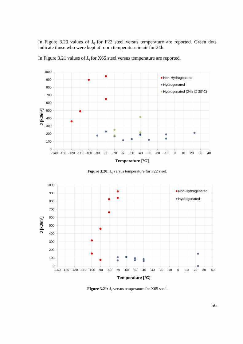
56

In Figure 3.20 values of Jq for F22 steel versus temperature are reported. Green dots indicate those who were kept at room temperature in air for 24h.

In Figure 3.21 values of Jq for X65 steel versus temperature are reported.

Figure 3.20: Jq versus temperature for F22 steel.

Figure 3.21: Jq versus temperature for X65 steel.

0

100

200

300

400

500

600

700

800

900

1000

-140 -130 -120 -110 -100 -90 -80 -70 -60 -50 -40 -30 -20 -10 0 10 20 30 40

J [k

J/m

2 ]

Temperature [°C]

Non-Hydrogenated

Hydrogenated

Hydrogenated (24h @ 30°C)

0

100

200

300

400

500

600

700

800

900

1000

-140 -130 -120 -110 -100 -90 -80 -70 -60 -50 -40 -30 -20 -10 0 10 20 30 40

J [k

J/m

2 ]

Temperature [°C]

Non-Hydrogenated

Hydrogenated

57

It was observed that, for tests that require more time compared to Charpy impact tests, hydrogen embrittlement is enhanced in both steels and it occurs at temperatures higher than those for impact tests, temperatures that can be reached in cold areas on earth.

If uncharged specimens at temperatures around -80°C, -90°C show high Jq values, that still depend on geometry, hydrogen charged specimen show a strong embrittlement, with values that drop until 100, 200 kJ/m2 at temperatures around -30°C, -40°C.

It must be said that Jq values are still high enough thanks to the good toughness properties of such materials.

It is interesting to split the elastic from the plastic part of Jq to better understand the loss of plasticity due to hydrogen.

Finally it should be pointed out that, also specimens kept at 30°C for 24h (green dots) show a remarkably reduction of toughness: this means that a relevant quantity of hydrogen was trapped inside other sites with a high activation energy.

In Figure 3.22 and Figure 3.23 plots of Jel and Jpl as a function of the test temperature are shown respectively for F22 and X65 steels.

Figure 3.22: plot of Jel e Jpl as a function of test temperature for F22.

0

100

200

300

400

500

600

700

800

900

1000

-140 -130 -120 -110 -100 -90 -80 -70 -60 -50 -40 -30 -20 -10 0 10 20 30 40

J [kJ

/m2]

Temperature [°C]

Jel - Non Hydrogenated

Jpl - Non Hydrogenated

Jel - Hydrogenated

Jpl - Hydrogenated

Jel - Hydrogenated (24h @ 30°C)

Jpl - Hydrogenated (24h @ 30°C)

58

Figure 3.23: plot of Jel e Jpl as a function of test temperature for X65.

It is evident form the two plots that for hydrogen charged specimen there is a relevant loss in plastic component. As matter of fact Jel is similar either for charged and uncharged specimens. This situation can be better shown by load-displacement graph from J tests. In Figure 3.24 and Figure 3.25 load curves are shown during the toughness test; for F22 curves at T = -80°C are shown while for X65 curve is taken at -70°C (F22 is tougher than X65).

0

100

200

300

400

500

600

700

800

900

1000

-140 -130 -120 -110 -100 -90 -80 -70 -60 -50 -40 -30 -20 -10 0 10 20 30 40

J [kJ

/m2]

Temperature [°C]

Jel - Non Hydrogenated

Jpl - Non Hydrogenated

Jel - Hydrogenated

Jpl - Hydrogenated

59

Figure 3.24: Load-displacement curve at T = -80°C for F22.

Figure 3.25: Load-displacement curve at T = -70°C for X65.

It is evident from these plots that, in charged specimens, there is no plastic contribution that should be present in such steels. The steel changes its mechanical properties and loses toughness.

To better investigate fracture surfaces after J test, a heat-tinting thermal treatment was performed on specimens where unstable growth occurred. This treatment consists in heating the sample at 300°C for 30 minutes, quenching in liquid nitrogen and the opening them in a brittle condition. In Figure 3.26 two different F22 specimens, after toughness, tests are compared: either hydrogen charged and uncharged.

0

10000

20000

30000

40000

50000

60000

0 0.25 0.5 0.75 1 1.25 1.5 1.75 2 2.25 2.5 2.75 3

Car

ico

[N]

Spostamento sulla linea di carico [mm]

Provini Non Caricati

Provini Caricati

Provini Caricati (24h @ 30 °C , test @ -70 °C)

0

10000

20000

30000

40000

50000

60000

0 0.25 0.5 0.75 1 1.25 1.5 1.75 2 2.25 2.5 2.75 3

Car

ico

[N]

Spostamento sulla linea di carico [mm]

Provini Non Caricati

Provini Caricati

Load-line displacement

Loa

d

Load-line displacement

Loa

d

Non Hydrogenated Hydrogenated

Non Hydrogenated

Hydrogenated

Hydrogenated (24h @ 30°C)

60

Uncharged specimen (F22) T = -100 °C

Jq = 890 kJ/m2

Δafinal = 0.5 mm

Charged specimen (F22) T = -90 °C

Jq = 179 kJ/m2 Δafinal = 2.5 mm

Figure 3.26: Images of fracture surfaces for F22 specimens after crack propagation in hydrogen and normal condition.

It can be observed that, in the uncharged specimen, crack propagation is limited due to a tough behavior; this is confirmed by a high value of Jq reached at the intersection with the 0,2 mm offset line. What happens in reality is a blunting (increase of the tip radius) of the crack tip due to plasticity without tearing of the material. On the other side, in presence of hydrogen, the crack propagations is broad and clear. This will be clarified in SEM fractographs analysis.

Test data are given in Appendix A.2.

3.5 Fatigue crack growth tests

In fracture mechanics fatigue crack propagation is usually described and studied through da/dN – ΔK log-log plots; da/dN is the crack growth rate per cycle and is plotted as a function of ΔK where:

max minK K K∆ = −

And K, the stress intensity factor is defined as follow:

61

K aβ σ π= ⋅ 3.10

Where:

− β is a dimensionless parameter depending on geometry of the specimen and the crack

− σ is the maximum stress, σmax, and then Kmax; or σmin and then Kmin − a is the crack length.

In Figure 3.27 a typical da/dN – ΔK log-log plot is depicted, there different regions can be pointed out:

region I: where a threshold value of ΔKth is defined below which there is no crack propagation or very slow crack growth;

region II: where there is a linear relation between crack growth and ΔK and Paris

law can be applied: mda C KdN

= ∆

region III: where crack growth increases rapidly to a limit value of ΔK where unstable propagation occurs, max CK K= .

Figure 3.27: Crack growth rate as a function of ΔK for steels.

62

Specimens used for this test are C(T) specimen with W equal to 40 mm. According to regulation from this dimension all other dimensions are obtained: a must be in a range between 0,2·W and 0,975·W.

During the whole test the following relation must be satisfied:

( )2

max

4 ys

KW a πσ

− ≥ ⋅

3.11

Crack propagation tests were carried out by varying the following parameter:

hydrogen presence in the specimen test temperature load frequency.

All tests were carried out accordingly to International regulation ASTM [42]. Tests were carried out in load control; it means that load applied by the machine to the specimen is a sinusoidal wave shaped with σmax and σmin ratio equal to R = 0,1. Measurements of crack growth were made through the compliance method. Precracking of the specimen was performed using these values of the load:

max 6800 F N=

min 680 F N=

It follows that R = 0,1. Clip on gage was used to measure the crack opening.

3.5.1 Tests on F22 steel

On F22 steels crack propagation tests were carried out for charged and uncharged specimens by varying temperature and frequency as stated above, using MTS 810 machine and the environmental chamber. It is well-known that hydrogen embrittlement is very dependent either on temperature and frequency [12] [43] .

In Table 3.11 the crack propagation test-plan is depicted, showing which test parameters were chosen to vary.

63

Table 3.11 Crack propagation test plan for F22 specimens.

Uncharged specimen Charged specimen 0,9÷1,3 ppm

T [ °C] Room temperature

-60 -100

Room temperature -30

f [Hz] 20 1

10

3.5.1.1 Fatigue crack growth on F22 uncharged specimens

In Figure 3.28 results from fatigue crack propagation tests are depicted. It should be immediately noticed that, for uncharged specimens, there is no temperature dependence since crack growth rate is not affected by temperature change; the curves are very similar, with the same slope and slightly differing in the y-intercept.

Propagation tests on uncharged specimens were carried out at a load frequency equal to f = 20 Hz. In these conditions, as widely shown in literature, frequency is not a parameter affecting growth rate.

64

Figure 3.28: Crack growth rate for uncharged specimens at different temperatures for F22 steel.

Paris coefficients have been calculated and are shown below:

9 3,191

3 3,167

60 , 1

9 3,174

100 , 1

2,3 10

2,1 10

1,9 10

roomT

H

T C f Hz

H

T C f Hz

da KdN

da KdN

da KdN

−

−

=− ° =

−

=− ° =

= ⋅ ⋅∆

= ⋅ ⋅∆

= ⋅ ⋅∆

It should be pointed out that variations between crack growth rates, at different temperatures, are very narrow and that crack growth rates at same ∆K, decrease while decreasing temperature, as expected. Indeed, cyclic plastic zone is reduced while decreasing temperature because yield strength is increased by temperature reduction.

y = 2E-09x3,1914 R² = 0,9958

y = 2E-09x3,1671 R² = 0,9841

y = 2E-09x3,1748 R² = 0,9718

1,E-06

1,E-05

1,E-04

1,E-03

1,E-02

10 100

da/d

N [m

m/c

ycle

]

∆K [MPa√m]

NoH T23 F20

NoH T-60 F20

NoH T-100 F20

65

3.5.1.2 Fatigue crack growth tests on hydrogen charged F22 specimens

In Figure 3.29, results from fatigue crack propagation tests on H-charged C(T) specimens, at room temperature, are depicted; two frequencies test were taken: at f = 1 Hz and f = 10 Hz. It is also shown the crack propagation curve for H-free F22 specimen for a better understanding of the phenomenon.

Figure 3.29: Crack growth rate for hydrogen-charged F22 specimens at different frequencies, T = 23°C.

The blue line indicates the test carried out at room temperature on H-free F22 specimen, it can be noted that there is a perfect connection between Paris theory and experimental data. It was also observed a linear and constant trend of the crack growth rate in the whole ΔK range. On the other hand, for hydrogen charged specimen tested at 10 Hz (orange and pink dots), a general increase in crack growth rate was observed at similar ΔK. In particular, at low ∆K and growth rates, embrittlement effect is clearly significant because of the high amount of hydrogen atoms reaching the crack tip. At higher values of ∆K, propagation rate meets again the values of uncharged curve. This phenomenon can be interpreted as it follows: crack growth rate is the result of a sum of two inputs (hydrogen effect and load effect), at low ΔK in a range ΔK = 15÷35 MPa√m hydrogen effect is predominant, while for higher values of ΔK mechanical propagation due to high loads becomes predominant. In the last case, the fatigue behavior is mainly controlled by the mechanical properties of the material (as if it were hydrogen free) since there is not enough time for hydrogen to reach the crack tip because of the high crack growth rate.

y = 2E-09x3,1914 R² = 0,9958

1,E-06

1,E-05

1,E-04

1,E-03

1,E-02

10 100

da/d

N [m

m/c

ycle

]

∆K [MPa√m]

NoH T23 F20

H T23 F1

H T23 F10_1

H T23 F10_2

66

Again, by observing Figure 3.29, the curve of H-charged specimen at 1Hz and room temperature shows a strong enhancement of the embrittling effect of almost two orders of magnitude when compared to the H-free curve. This can be explained by the fact that the crack tip spends longer time at maximum load since, as shown in paragraph 2.2.3, hydrostatic stress segregates H. It was observed that crack growth is somehow independent from load condition ΔK since it propagates at a constant rate. As a matter of fact, ΔK is not that important since embrittlement effect occurs at a constant and remarkable growth rate.

Figure 3.30: Crack growth rate for hydrogen-charged F22 specimens at different frequencies, T = -30°C.

In Figure 3.30, test results for H-charged specimens, tested at T = -30°C and at 1Hz and 10Hz frequencies, are depicted.

Also at this test temperature, it was observed a horizontal trend for the charged specimens; nevertheless it was noted a smaller embrittling effect of the hydrogen; for analogous frequencies, owing to low temperature, there is a slowdown of hydrogen diffusion at the crack tip. Especially at high ΔK values, for tests carried out at -30°C and f = 10 Hz on charged specimens, it was observed that the crack growth rate approaches the uncharged curve. This fact shows that hydrogen influence on crack growth rate is reduced compared to tests carried out at T = 23°C. In Figure 3.31 all results on F22 specimens are depicted together in order to give a better display of the trend and dependence of hydrogen embrittlement on frequency and temperature.

y = 2E-09x3,1914

1,E-06

1,E-05

1,E-04

1,E-03

1,E-02

10 100

da/d

N [m

m/c

ycle

]

∆K [MPa√m]

NoH T23 F20

H T-30 F1_1

H T-30 F1_2

H T-30 F10_1

H T-30 F10_2

67

Figure 3.31: fatigue crack propagation test results on F22 charged and uncharged specimens at different temperatures and frequencies.

Crack growth coefficients extrapolated according to Paris theory are given below, it can be noted that Paris relation fails on H-charged materials since coefficient are not those typical of steels:

9 3,191

3 0,2391 6 1,285

, 1 , 10

4 0.03504

30 , 1

2,3 10

1, 2 10 5 10

7,9 10

room

room room

NoH

T

H H

T f Hz T f Hz

H

T C f Hz

da KdN

da daK KdN dN

da KdN

−

− −

= =

−

=− ° =

= ⋅ ⋅∆

= ⋅ ⋅∆ = ⋅ ⋅∆

= ⋅ ⋅∆

4 0,1823

30 , 10

2,6 10H

T C f Hz

da KdN

− −

=− ° =

= ⋅ ⋅∆

Differences of these values are clearly noticeable by comparing test results at different temperature. It was also observed a good reproducibility of results on long time tests. It can be noted that, in H-charged specimen, m exponent tend to zero. This fact means that crack growth rate reaches a plateau and at the same time, since it is not equal to zero, there is still a contribution from the mechanical fatigue growth.

1,E-06

1,E-05

1,E-04

1,E-03

1,E-02

10 100

da/d

N [m

m/c

ycle

]

∆K [MPa*m1/2]

NoH T23 F20NoH T-60 F20NoH T-100 F20H T23 F1H T23 F10_1H T23 F10_2H T-30 F1_1H T-30 F1_2H T-30 F10_1H T-30 F10_2

68

In Figure 3.32 crack length as a function of cycle number is shown.

Figure 3.32: Crack length as a function of number of cycles for F22 steel.

It is evident the change of propagation rate when hydrogen is present; by looking at the number of cycles to failure, it can be noted that, for a hydrogen charged specimen tested at room temperature and 1Hz, this value is equal to 5.500 cycle; while, for a hydrogen free specimen this value is equal to 340.000 cycles. This fact means that crack growth rate is 60 times faster in the hydrogen charged specimen and it should be taken into account anytime these conditions are present.

3.5.2 Tests on X65 steel

Also on X65 steel, crack propagation tests were carried out for H-charged and uncharged specimens by varying temperature and frequency as done with F22 specimens. In Table 3.12 and Table 3.11, crack propagation test-plan is depicted, showing which test parameters were chosen to vary.

18

22

26

30

34

38

0 100.000 200.000 300.000 400.000

Cra

ck le

ngth

[mm

]

Number of cycles

NoH T23 F20_1NoH T23 F20_2H T23 F1H T23 F10_1H T23 F10_2H T-30 F1_1H T-30 F1_2H T-30 F10_1H T-30 F10_2

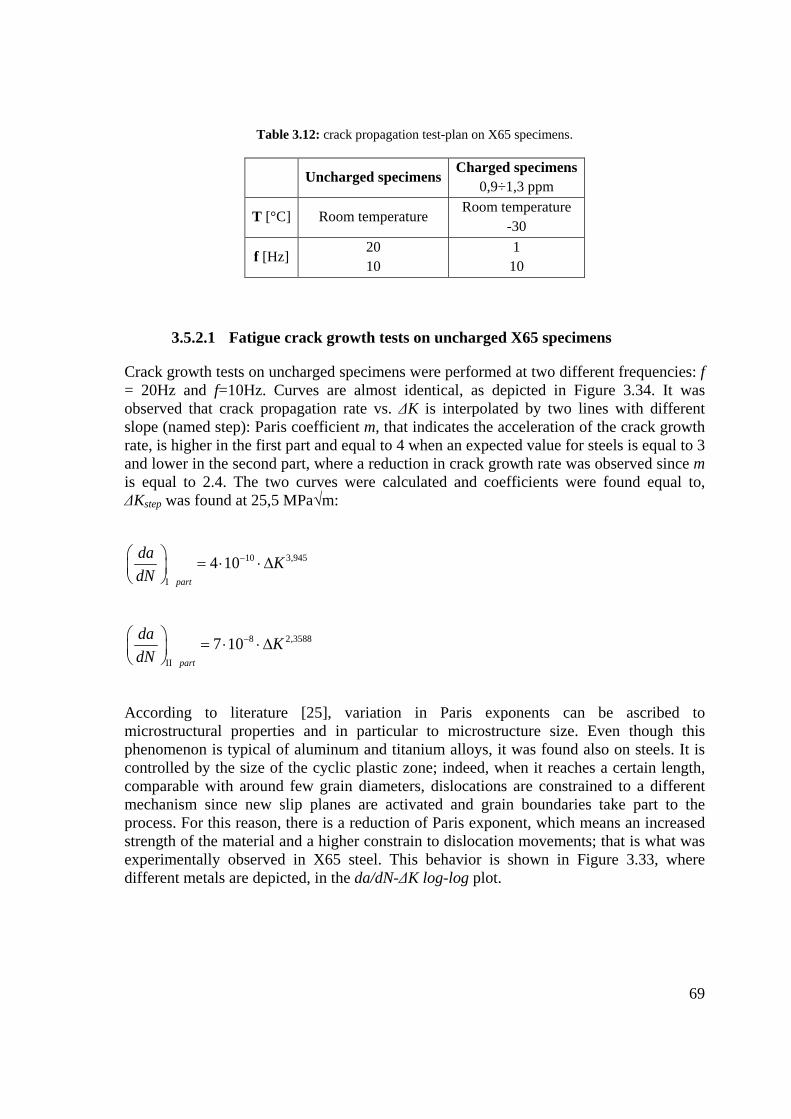
69

Table 3.12: crack propagation test-plan on X65 specimens.

Uncharged specimens Charged specimens 0,9÷1,3 ppm

T [°C] Room temperature Room temperature

-30

f [Hz] 20 10

1 10

3.5.2.1 Fatigue crack growth tests on uncharged X65 specimens

Crack growth tests on uncharged specimens were performed at two different frequencies: f = 20Hz and f=10Hz. Curves are almost identical, as depicted in Figure 3.34. It was observed that crack propagation rate vs. ΔK is interpolated by two lines with different slope (named step): Paris coefficient m, that indicates the acceleration of the crack growth rate, is higher in the first part and equal to 4 when an expected value for steels is equal to 3 and lower in the second part, where a reduction in crack growth rate was observed since m is equal to 2.4. The two curves were calculated and coefficients were found equal to, ΔKstep was found at 25,5 MPa√m:

10 3,9454 10part

da KdN

−

Ι

= ⋅ ⋅∆

8 2,35887 10part

da KdN

−

ΙΙ

= ⋅ ⋅∆

According to literature [25], variation in Paris exponents can be ascribed to microstructural properties and in particular to microstructure size. Even though this phenomenon is typical of aluminum and titanium alloys, it was found also on steels. It is controlled by the size of the cyclic plastic zone; indeed, when it reaches a certain length, comparable with around few grain diameters, dislocations are constrained to a different mechanism since new slip planes are activated and grain boundaries take part to the process. For this reason, there is a reduction of Paris exponent, which means an increased strength of the material and a higher constrain to dislocation movements; that is what was experimentally observed in X65 steel. This behavior is shown in Figure 3.33, where different metals are depicted, in the da/dN-ΔK log-log plot.

70

Figure 3.33: Schematic for the effect of cyclic plastic zone size on the fatigue crack growth rate curve: T = transitions influenced by the relation between cyclic plastic zone size and microstructure [25].

Figure 3.34: Crack growth rate for uncharged specimens at different temperatures for X65 steel.

3.5.2.2 Fatigue crack growth tests on charged X65 specimens

In Figure 3.35 results from fatigue crack growth tests, at room temperature on H-charged specimens, are depicted; two frequencies test were taken: at f = 1 Hz and f = 10 Hz. Test frequencies were taken similarly to F22 tests.

y = 4E-10x3,945 R² = 0,9405

y = 7E-08x2,3588 R² = 0,9425

1,E-06

1,E-05

1,E-04

1,E-03

1,E-02

10 100

da/d

N [m

m/c

yce]

∆K [MPa*m1/2]

NoH T23F20_aNoH T23F20_b

71

Figure 3.35: Crack growth rate for hydrogen-charged X65 specimens at different frequencies, T = 23°C.

Hydrogen effect causes an embrittlement and a crack growth acceleration comparable with the one observed during F22 testing. Plateau regions are easily noticeable for both test frequencies, 1Hz and 10 Hz; also, as stated above, crack growth rate reaches a constant value independent from crack length and load level, since it is independent from ∆K. In Figure 3.36, results for specimens tested at T = -30°C and similar frequencies are depicted. Also at this test temperature, it was observed a horizontal trend for the charged specimens; nevertheless, it was noticed a smaller embrittling effect of the hydrogen; for analogous frequencies. This fact can be explained with thermal considerations: at lower temperatures, there is a slowdown of hydrogen diffusion reaching the FPZ (fracture process zone). Especially at high ΔK values, for tests carried out at -30°C and f = 10 Hz on charged specimens, it was observed that the crack growth rate approaches the uncharged curve. This fact shows that hydrogen influence on crack growth rate is reduced compared to tests carried out at T = 23°C.

y = 4E-10x3,945 R² = 0,9405

y = 7E-08x2,3588 R² = 0,9425

1,E-06

1,E-05

1,E-04

1,E-03

1,E-02

10 100

da/d

N [m

m/c

ycle

]

∆K [MPa*m1/2]

NoH T23 F20_aNoH T23 F20_bH T23 F1_1H T23 F1_2H T23 F10_1H T23 F10_2

72

Figure 3.36: Crack growth rate for hydrogen-charged X65 specimens at different frequencies, T = -30°C.

In this case, temperature plays a very important role in hydrogen embrittling effect; indeed, hydrogen diffusivity inside the lattice decreases and da/dN-∆K curves approach the uncharged material behavior. As it can be noted, in same ∆K range of where, at room temperature, there is a plateau in the curve at T = -30°C, there is a positive slope.

Also, in the curve at T = -30°C and f = 1Hz, it is well-noticeable how hydrogen embrittling effect has a maximum at middle ∆K range, while, for lower and higher values material behavior meets again the uncharged curve, that is the typical fatigue behavior of the material without hydrogen. It means that, if hydrogen embrittlement assisted cracking on crack growth were not taken into account, the most surprising and catastrophic damages can occur at medium ∆K range, since in this range deviation form expected behavior is maximum.

In Figure 3.37 and Figure 3.31, all results on X65 specimens are depicted in order to give a better display of the trend and dependence of hydrogen embrittlement on frequency and temperature.

y = 4E-10x3,945 R² = 0,9405

y = 7E-08x2,3588 R² = 0,9425

1,E-06

1,E-05

1,E-04

1,E-03

1,E-02

10 100

da/d

N [m

m/c

ycle

]

∆K [MPa*m1/2]

NoH T23 F20_aNoH T23 F20_bH T-30 F1_1H T-30 F1_2H T-30 F10_1H T-30 F10_2

73

Figure 3.37: fatigue crack propagation test results on X65 charged and uncharged specimens at different

temperatures and frequencies.

Crack propagation equations and coefficients for the X65 curves are given below:

10 3,945 8 2,3588

, ,

3 0,0101 4 0,3593

, 1 , 10

3

4 10 7 10

2,3 10 2 10

room room

room room

H H

T Part T Part

H H

T f Hz T f Hz

T

da daK KdN dN

da daK KdN dN

dadN

− −

Ι ΙΙ

− −

= =

=−

= ⋅ ⋅ ∆ = ⋅ ⋅∆

= ⋅ ⋅ ∆ = ⋅ ⋅∆

6 1,724 5 0,561

0 , 1 30 , 10

4 10 4 10H H

C f Hz T C f Hz

daK KdN

− −

° = =− ° =

= ⋅ ⋅ ∆ = ⋅ ⋅∆

For hydrogen charged specimens, the calculation of Paris coefficient were done by considering the plateau region; as already discussed for F22, m coefficient approaches zero values at T room and low frequencies.

In Figure 3.38 crack length as a function of cycle number is shown.

y = 4E-10x3,945 R² = 0,9405

y = 7E-08x2,3588 R² = 0,9425

1,E-06

1,E-05

1,E-04

1,E-03

1,E-02

10 100

da/d

N [m

m/c

ycle

]

∆K [MPa*m1/2]

NoH T23 F20_aNoH T23 F20_bH T23 F1_1H T23 F1_2H T23 F10_1H T23 F10_2H T-30 F1_1H T-30 F1_2H T-30 F10_1H T-30 F10_2

74

Figure 3.38: Crack length as a function of number of cycles for X65 steel.

As previously noted with F22 tests, when specimen are hydrogen charged, unstable propagation is reached 30 times faster than the uncharged one; the maximum enhancement is observed if comparing data for a hydrogen charged specimen at room temperature and f = 1 Hz and the uncharged one. As it will be shown later, maximum enhanced of hydrogen embrittlement appears at room temperature.

3.5.3 Remarks on results

A common feature that emerged from data is the presence of a transient and/or a large scatter of data at the beginning of the test until a certain, threshold, ΔKth level. This threshold appears to be increased by frequency and decrease by increasing temperature, In particular this threshold seems lower for F22 steel (around 20 MPa√m, as it can be noted from Figure 3.31) and slightly higher for X65 steel( around 23 MPa √m, see Figure 3.37). After this transient, behavior of the material seems more stable. It is difficult to assess quantitatively this transient since accurate tests need to be performed, nevertheless a better understanding will be provided in next chapter thanks to fractographic investigation and comparison with literature and theory shown in chapter 2. Another remark, that should be done, concerns the fact that specimen have been hydrogen precharged; in literature many of these tests are done under cathodic reaction (by varying the potential) of H so that results seem more like stress corrosion cracking (SCC) while in this work results are typical of HE of charged lattice.

20

24

28

32

36

0 50.000 100.000 150.000

Cra

ck le

ngth

[mm

]

Number of cycles

NoH T23 F10H T23 F1_1H T23 F1_2H T23 F10_1H T23 F10_2H T-30 F1_1H T-30 F1_2H T-30 F10_1H T-30 F10_2

75

4 Fatigue crack growth predicting model

4.1 Theory of the model

In this chapter, a model to predict the hydrogen embrittlement crack growth rate in the II region of the da/dN – ΔK log-log plot is suggested. This model will predict the behavior of the material as a function of the experimental parameters such as: test temperature, load frequency and ΔK. In particular, once it is known the material behavior without hydrogen and how hydrogen enhances embrittlement, it is possible to predict the crack growth rate and therefore the crack length after a certain number of cycles at constant load for a certain temperature and load frequency. This model rests on a superposition of effects: mechanical fatigue crack growth and purely hydrogen embrittled sustained growth, as given in [26] and revised in [44].

Fatigue crack growth in aggressive environments can be enhanced by sustained load fracture during each load cycle. There are two main models which try to account for this effect:

Superposition model, reference [44] and given in Eq. 4.1; The process competition model, reference [45] and given in Eq. 4.2.

The superposition model proposes that the overall crack growth rate is the sum of a baseline fatigue component (mechanical fatigue) and a component due to sustained load fracture (as in Figure 1.8). On the other hand, the process competition model assumes that fatigue and sustained load fracture are mutually competitive and that the crack will growth at the fastest available rate, whether that is the baseline fatigue crack growth rate or the crack growth rate per cycle owing to sustained load fracture. Models are formulated as it follows:

76

superposition model ( )ITOT B

da da da K t dtdN dN dt

= + ∫

4.1

process for ( )

competition model

= ( ) for ( )

ITOT B B

I I

da da da da K t dtdN dN dN dt

da daK t dt K t ddt dt

= > ∫

∫B

datdN

> ∫

4.2

B stands for baseline fatigue (mechanical fatigue) and the integral in Eq. 4.1 and 4.2 is taken over one cycle of the fatigue loading and incorporates the effect of frequency, f, and stress ratio, R, via KI(t).

In this experimental investigation, it was found from SEM analysis (next chapter) that, in the fracture surface, it can be spotted either the base mechanical fatigue (striations) and the sustained load fracture (facets and cells with inclusion inside). For this reason, superposition model was taken into account and applied.

4.1.1 Frequency dependence

The following derivation will be done for superposition model, for the reason already mentioned; since in this investigation stress ratio was not considered and important parameters are temperature and frequency, it is possible to simplify the integral in Eq. 4.1 and 4.2 and give to it a physical meaning as it follows:

1( ) with ( )I IIHAC IHAC

da da da da da daK t dt dt t K tdt dt dt dt f dt dt

≅ ⋅ = ⋅ = ⋅ ≅

∫ ∫ ∫

Where IHAC

dadt

is the average sustained load fracture rate owing to internal hydrogen

assisted cracking and, since the integral in Eq. 4.1 was calculated over one loading cycle, 1tf

= .

Hence, the superposition model, given in Eq. 4.1, can then be rearranged as it follows:

77

1 TOT B IHAC

da da dadN dN f dt

= + ⋅

4.3

Hence, the superposition of both crack growth rates (i.e. baseline and IHAC) should give the frequency dependence of the overall crack propagation rate (TOT) once the behavior in the II region of the H-free material and the average sustained load fracture rate

IHAC

dadt

are known.

Figure 4.1 is a schematic of how the superposition model can be used to predict the overall crack growth rate curve for the materials in specific environmental and load conditions. It is also shown that there might be a Kstart at which IHAC is null before and contributes after this level to crack growth; this behavior was found also in tests data, nevertheless, accurate measurements need to be done in order to have a precise explanation of the phenomenon in a quantitative way; in the fractographic investigation this point will be better explained.

Figure 4.1: Superposition model.

It can also be seen that the crack propagation due to hydrogen embrittlement is independent from ∆K in a certain range, between ∆Kstart, where hydrogen presence starts to affect the material and higher ∆K where crack propagation is no longer dependent on hydrogen embrittlement since mechanical growth is much higher and the material is approaching instability, this behavior was found also in this analysis and that is the reason why it was possible to simplify the integer in Eq. 4.1. There are other models that calculate da/dt as a function of intrinsic parameters of the material such as elastic modulus, yield strength, strain hardening coefficient, diffusion coefficient, grain and inclusion size, hydrogen content and adjusting the value according to semi-empirical values. Nevertheless, these measurements take a long time and in this case some of them are not available: they require exact values of microscopic properties and diffusivity as well as hydrogen distribution and concentration in the specimen and they all require adjustable parameters. For these reasons they result difficult and not always reliable to be applied in real cases.

78

4.1.2 Temperature dependence

Modeling crack growth rate according to temperature is very important, since the goal of the research is to study temperature dependence. First of all, a wide bibliographic research was done, in order to understand the mechanisms and analyze previous experimental models. As shown in paragraph 2.2, diffusion is one of the controlling parameter of HE and since diffusion is governed by an Arrhenius relation with temperature, investigation was conducted on this way. From Eq. 4.3 and from tests on uncharged specimens, it was shown that crack growth rate does not depend either on temperature and frequency, so the term that accounts for temperature should be the sustained load crack growth due to internal hydrogen assisted cracking da/dt. In Troiano’s researches [8], empirical relations between da/dt sustained load fracture growth rate and other parameters (temperature and H2 pressure, see Figure 4.2) were shown. Since, in his researches, H was fed by gas atmosphere and in this work H is pre-charged, there was the need to find conditions that could be compared to this case. In reference [8], it was found that crack growth was proportional to the square root of H pressure and diffusivity in conditions where the controlling rate was the diffusion of H into the FPZ, (“at high pressure both gas phase transport and surface reaction are sufficiently fast to maintain an adequate supply of hydrogen [8]”) as it follows:

0 exp2

a

II

Eda p D pDdt RT

∝ = −

4.4

Where p is the H pressure in the atmosphere surrounding the specimen (in Troiano researches, an H atmosphere was used to charge the specimen, Hp C∝ according to Sievert’s law [46]) and D is the diffusivity as explained in section 2.2.1. The apparent activation energy for crack growth, therefore, would be equal to one-half that for diffusion Ea.

Since there is proportionality in Eq. 4.4, this model is primarily useful to estimate relative response to changes in environmental conditions and, since it does not contain any explicit metallurgical parameters, it cannot provide estimates of absolute rates for a given alloy.

Stage II crack growth dependence on temperature is well depicted in Figure 4.2; it can be seen that this relationship has a maximum at room temperature T = 300 K, and, above this temperature, crack growth drops. This experimental data was found in many investigations and it seems verified that hydrogen embrittlement maximum enhancement is reached at the room temperature. The reason can be found in the models shown in chapter 2: it is due to reduced H accumulation at damage sites within the FPZ. Indeed, according to Eq. 2.12, H segregation owning to lattice dilatation from hydrostatic stresses reduces with increasing temperature and according to Eq. 2.8 the amount of H trapped decreases with increasing temperature while diffusivity increases with temperature: break-even is then

79

reached at room temperature. As mentioned before, since this model contains proportionality, another viable approach lies on considering crack growth ratios at different temperatures, through Eq. 4.4. Thanks to this approach, all parameters that do not depend on temperature are canceled (diffusion coefficient D0 and hydrogen concentration) and temperature dependence is preserved. The adjustable parameter then is the activation energy of the process that should be divided by 2 according to Troiano. Hence for any T temperature, it can be written:

( )( )

23 exp 2 ( 296 )

exp 2

T C a

IHACT

aIHAC

Eda dt R T K

Eda dt RT

= ° − = = −

( ) 23exp 2 ( 296 )

exp 2 ( [ ])

aTT C

IHACaIHAC

ER T Kda da dt

EdtR T K

= ° − = = ⋅

−

4.5

Figure 4.2: The temperature dependence of the Stage II K-independent subcritical crack growth rate for IHAC in tempered martensitic 4340 steel (σYS = 1660 MPa), H precharged (CH-TOT = 3 ppm or more) and

tested at fixed load in moist air. The bars represent experimental measurements and the solid line is the model prediction using a H-trap binding energy of Hb =EB = 27 kJ/mol [7].

80

4.2 Analytical procedure

For both steels, it was first pointed out the “Paris relation” of the uncharged steel; it has been found that for F22 material constants are:

92,3 10 /3,1914

C mm cyclem

−==

For X65, two different equations were used as mentioned in paragraph 3.5.2.1, Paris coefficients then are:

94, 2 10 / 25,5

3,9450C mm cycle

K MPa mm

−Ι

Ι

=∆ <

=

And for the second part:

87 10 / 25,5

2,3588C mm cycle

K MPa mm

−ΙΙ

ΙΙ

= ⋅∆ >

=

Then, the average crack growth rate per cycle owning to the hydrogen embrittlement was estimated. Calculations were done by taking as reference either T = 23°C and f = 1 Hz or the average of crack rates at different frequencies, using the following relation:

TOT BIHAC

da da da fdt dN dN

= − ⋅

4.6

Analytically, determination of the average crack growth rate per cycle owning to the hydrogen embrittlement was found according to Eq. 4.6, by subtracting the data on the uncharged steel ( )/

Bda dN that is Paris relation to ( )/

TOTda dN of the charged specimen

at the same ΔK in a range where still the IHAC effect is predominant (plateau region).

When crack propagation rate is much higher than the uncharged material the estimation can be performed by dividing the crack growth length and the elapsed time that this process takes in the plateau region of the specimens charged, with hydrogen and tested at 1 Hz. The reason why it was consider only this region is that in the plateau the hydrogen embrittlement contribution to crack growth is relevant compared to the uncharged (almost 2 orders of magnitude); analytically, the calculation can be done as it follows:

81

IHAC

plateau

da aNdtf

∆ = ∆

4.7

In our analysis, in order to obtain a more precise calculation, Eq. 4.6 was used instead of Eq. 4.7.

Another parameter that should be estimated to a good fitting of the model is ∆Kstart , that is the value of ∆K where crack propagation in presence of hydrogen, begins to be influenced and increases.

( ) ( )· 1startIstart

K K R∆ = − 4.8

Following considerations come from observation of data but are not showed in the models since evidences and data are not enough to assess it clearly, nevertheless they are useful in case needed. Indeed, since hydrogen embrittling acceleration occurs when a critical hydrogen concentration at the crack tip is reached, this estimation should be done according to a micromechanical model that takes into account the hydrogen diffusion and kinetics in the FPZ (fracture process zone) and other variables (Ccr, C0, T, D, ry, σH). In the prediction, a simple reasoning can be done: from tests it was noticed that ΔKstart is temperature and frequency dependent and for both temperatures is in the range of 12,5 - 14,5 MPa√m so it was adjusted according to data. Finally it can be assumed that the upper boundary of the model reaches asymptotically the ΔKIC of the material. Nevertheless, since data are not available and no tests have been done to measure threshold and critical level, they will not be shown in the model plot even though either from literature and data there is a very similar trend.

Since the model predicts a superposition of effect and not a competition there must be, and it was experimentally observed, a transient where hydrogen assisted cracking approaches

the EAC

dadt

rate in a range of ΔK from the threshold to the plateau.Transient can be be

modeled thanks to experimental data. In order to avoid a step at ∆Kstart in the crack growth rate it can be choose to gradually introduce the effect of hydrogen embrittlement after this point; that corresponds from data to an interval in ΔK=2 MPa√m in which the

contribution of EAC

dadt

is gradually introduced from 0 to 1; Eq. 4.4 was then modified

as it follows:

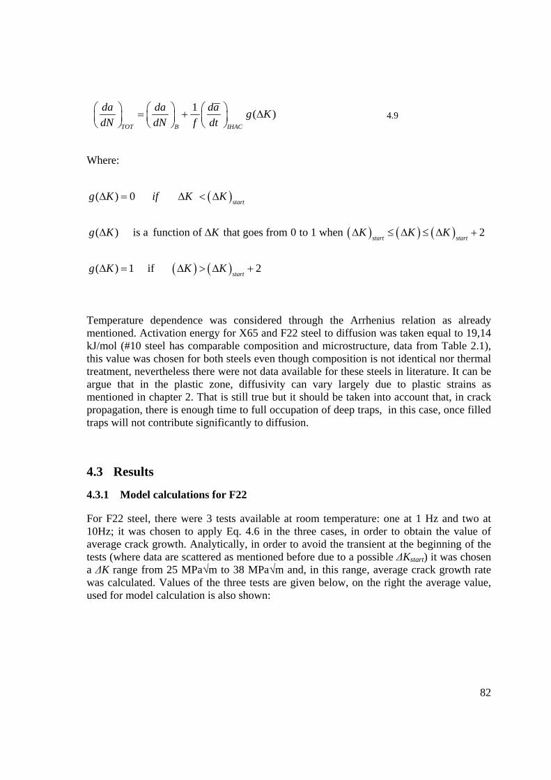
82

1 ( )TOT B IHAC

da da da g KdN dN f dt

= + ∆

4.9

Where:

( )

( ) ( ) ( )

( ) ( )

( ) 0

( ) is a function of that goes from 0 to 1 when 2

( ) 1 if 2

start

start start

start

g K if K

g K K

g

K

KK

K

K K

K

∆ = < ∆

∆ ∆ ≤ ∆

∆ > ∆

∆

∆ ∆ ≤ +

∆ = +

Temperature dependence was considered through the Arrhenius relation as already mentioned. Activation energy for X65 and F22 steel to diffusion was taken equal to 19,14 kJ/mol (#10 steel has comparable composition and microstructure, data from Table 2.1), this value was chosen for both steels even though composition is not identical nor thermal treatment, nevertheless there were not data available for these steels in literature. It can be argue that in the plastic zone, diffusivity can vary largely due to plastic strains as mentioned in chapter 2. That is still true but it should be taken into account that, in crack propagation, there is enough time to full occupation of deep traps, in this case, once filled traps will not contribute significantly to diffusion.

4.3 Results

4.3.1 Model calculations for F22

For F22 steel, there were 3 tests available at room temperature: one at 1 Hz and two at 10Hz; it was chosen to apply Eq. 4.6 in the three cases, in order to obtain the value of average crack growth. Analytically, in order to avoid the transient at the beginning of the tests (where data are scattered as mentioned before due to a possible ΔKstart) it was chosen a ΔK range from 25 MPa√m to 38 MPa√m and, in this range, average crack growth rate was calculated. Values of the three tests are given below, on the right the average value, used for model calculation is also shown:

83

1 ,

32, 46 10 /roomHz T

IHAC

d a mm sdt

− = ⋅

32,33 10 /roomT

IHAC

da mm sdt

− = ⋅

10 ,

32,80 10 /roomHz T

IHAC

da mm sdt

− = ⋅

10 ,

31,73 10 / (b)roomHz T

IHAC

da mm sdt

− = ⋅

The average rate, given in the right side, is of the same order and very similar to half of the mean diffusion length in half of the cycle time; indeed, analyzing the equation and, using for diffusion, data from Table 2.1, these values are very close:

3

2 2 with / 2 0,5 and T=23°C

2, 4 10 [ ]2

ave

ave

l D t t

l mm−

= ⋅ ⋅ =

= ⋅

This is a further evidence of diffusion controlled mechanism and provides a first approximation to the crack growth rate.

Model was then applied to F22 data; results at 23°C and different load frequencies were compared with test data as it can been seen from the overlapping in Figure 4.3.

84

Figure 4.3: Model prediction and experimental data at room temperature for F22 steel.

ΔK start and maximum ΔK were not inserted in the model since they require accurate tests to be calculated; at the beginning of the tests there is a deviation between model and data that can be due either to start-up and hydrogen loss during operations before testing or to the ΔKstart as it will be shown in next chapter. For these reasons, considerations on ΔK start seem to be too daring.

As it can be seen, the model predicts effectively, real material behavior at 10 Hz and, according to the theory reasoning, it is reliable certainly in the tested range. Prediction at 10 Hz, can be done without any data at that frequency, by using data t 1Hz. In Figure 4.3, it is also shown the predicted behavior of the material tested at 2 Hz.

Next step was to apply the thermal model, given in Eq. 4.5 to crack growth rate, at T = -30°C in order to verify how good the prediction could be. It should be pointed out that from Eq. 4.4, the parameter affecting rate ratio is the activation energy for the process that according to Troiano’s researches it should be divided by 2, since of the square root proportionality.

According to Eq. 4.5 and data for diffusion of Ea equal to 19,71 kJ/mol crack growth rate at -30°C is equal to:

1,E-06

1,E-05

1,E-04

1,E-03

1,E-02

10

da/d

N [m

m/c

ycle

]

∆K [MPa⋅m1/2]

Model 1HzModel 2HzModel 10HzParis lawTest data H-freeTest data 1HzTest data 10HzTest data 10Hz b

85

30

49,74 10 T C

IHAC

da mmdt s

=− °

− = ⋅

Figure 4.4: crack growth rate da/dt due to hydrogen effect as a function of temperature for F22 steel.

In Figure 4.4, thermal model has been applied to F22 with activation energy equal to 19,71 kJ/mol, the crack growth rate, in log scale, is plotted versus the inverse of absolute temperature as done also in Figure 4.2. The plot was not interpolated for temperature above room temperature since in literature it was found a decreasing trend after this point. With data at T = -30°C and at different frequencies it was possible to obtain the average crack growth rate owing to hydrogen; the calculation was done as for data at T = 23°C and results are the following:

1,0E-04

1,0E-03

1,0E-023 3,5 4 4,5 5

da/d

t [m

m/s

]

1000/T[K]

Model data

Test data

86

1 , 30

47,67 10 /Hz T C

IHAC

da mm sdt

=− °

− = ⋅

30

47,86 10 /T C

IHAC

da mm sdt

=− °

− = ⋅

1 , 30

48,17 10 / (b)Hz T C

IHAC

da mm sdt

=− °

− = ⋅

10 , 30

47,74 10 /Hz T C

IHAC

da mm sdt

=− °

− = ⋅

The calculated values and data at T = -30°C are depicted in Figure 4.5; the model can be also reversed to obtain activation energy for perfect fitting, that is what has been done below.

It can be noted a good approximation between test data and thermal model prediction. From tests on propagation, carried out at T = -30°C, crack growth rate da/dt is equal to 7,86·10-4 mm/s. The difference between the predicted rate and analytically calculated rate (equal to 9,74·10-4 mm/s), can be due to low accuracy of activation energy Ea, to low accuracy during crack growth testing rate and to a lack of accuracy in H concentration in the lattice; in fact by reversing the model it is possible to estimate the activation energy by imposing a perfect fitting of the model, the result is equal to 25 kJ/mol, higher than the value from literature and almost identical to the one used in Figure 4.2 (equal to 27 kJ/mol, activation energy for trap diffusion). Subsequently this calculation, it was possible to plot the crack propagation curves at T = -30°C using the model. In Figure 4.5 the curves are shown; also in this case model prediction is satisfactory.

87

Figure 4.5: crack propagation curves prediction at T = -30°C and different frequencies for F22 steel, crack growth rate has been calculated via thermal model.

It can be noted that, in the test data at 10Hz there is a lack of prediction. While, for the data at 1Hz there is a very good fitting either using thermal model 4.3 or calculation 4.5 from data at T = -30°C.

4.3.2 Model calculations for X65

For X65 steel, calculations were done using both Paris coefficients set and the procedure was similar to the one of F22 steel. Fatigue crack growth rate due to hydrogen effect was calculated and gave the following values that can be seen also in Figure 4.6.

1 , 1 ,

3 3

10 ,

3

2,54 10 / 2,05 10 / (b)

3,35 10 /

room room

room

Hz T Hz T

IHAC IHAC

Hz T

IHAC

da damm s mm sdt dt

da damm sdt d

− −

−

= ⋅ = ⋅

= ⋅

10 ,

33,18 10 / (b)roomHz T

IHAC

mm st

− = ⋅

1,E-06

1,E-05

1,E-04

1,E-03

1,E-02

10

da/d

N [m

m/c

ycle

]

∆K [MPa⋅m1/2]

Model prediction and test data at T = -30°C for F22

Model 1HzModel 2HzModel 10HzParis lawTest data H-freeTest data 1HzTest Data 1Hz bTest data 10Hz

88

The average crack growth rate due to hydrogen assisted cracking that is used for model prediction is equal to:

32,77 10 / roomT

IHAC

da mm sdt

− = ⋅

This value is slightly higher than that found for F22, indicating that both steels are equally susceptible to hydrogen embrittlement.

Model prediction at T = 23°C and different frequencies was compared with test data; in Figure 4.6 the superposition of model prediction and test data are shown, considering Paris coefficient and the calculated rate.

Figure 4.6: Model prediction and test data for X65 at 23°C.

As it can be seen, the model predicts effectively, real material behavior at 10 Hz and, according to the theory reasoning, it is reliable certainly in the tested range. As previously noticed for F22, also X65 shows a scattering of data at the beginning of tests, in particular data at 10Hz are scattered homogeneously around a mean value while for data at 1Hz there is an increasing trend, that approaches the predicted value.

Then, fatigue crack propagation rate at T = -30°C was calculated according to Eq. 4.5 and Ea = 19,71 kJ/mol; it resulted equal to:

1,E-06

1,E-05

1,E-04

1,E-03

1,E-02

10

da/d

N [m

m/c

ycle

]

∆K [MPa⋅m1/2]

Model prediction and test data at T = 23°C for X65

Model 1HzModel 2HzModel 10HzParis lawTest data H-freeTest data 1HzTest data 1Hz bTest data 10Hz bTest data 10Hz

89

30

31,16 10

T C

IHAC

d a mmdt s

=− °

− = ⋅

In Figure 4.7, crack growth rate versus temperature for X65 steel at 1Hz is depicted. In this case, activation energy for diffusion equal to 26 kJ/mol was used instead of 19,71 kJ/mol, indeed best fitting was found at this activation energy and that is also very similar to reference data shown in Figure 4.2.

Also, average crack growth rate was calculated through fatigue crack growth data at T = -30°C according to Eq. 4.2, result is:

30

48,94 10

T C

IHAC

d a mmdt s

=− °

− = ⋅

Obtained from the average of the following values, from the three specimens tested at T = -30°C:

1 , 30 1 , 30

4 3

10 , 30

4

5,74 10 / 1, 41 10 / (b)

6,96 10 /

Hz T C Hz T C

IHAC IHAC

Hz T C

IHAC

da d amm s mm sdt dt

da mm sdt

=− ° =− °

− −

=− °

−

= ⋅ = ⋅

= ⋅

90

Figure 4.7: crack propagation rate in plateau region as a function of temperature at 1Hz for X65 steel.

Once again the difference between data and model prediction is very small and it can be ascribed to accuracy in determining Ea, also in can be noted that there is some discrepancy between specimens tested at same temperature and frequency conditions, this might be due to different hydrogen content that cannot be verified once the test is performed.

Also for this case, model was tested with data for the whole ΔK tested range; once again results are matching real behavior. The model shows, once again, a good reproducibility of the test data, in Figure 4.8 model and test data for X65 at -30°C are depicted.

1,0E-04

1,0E-03

1,0E-023 3,5 4 4,5 5

da/d

t [m

m/s

]

1/T[K]·103

Model data

Test data

91

Figure 4.8: Model prediction and experimental data at T=-30°C for X65.

It should be noted that, even though no data are available at -30°C and 10 Hz (violet dots in Figure 4.8), the model predicts with high accuracy the behavior of the material; once again the transient was not considered for lack of test data. It should be noticed that, even though some inaccuracy in test data at same test condition, the model agrees with the material behavior. At the end of this chapter, further remarks on results will be given.

4.4 Application of the model to a real crack-like defect in pipelines

4.4.1 Application of the model to a real case (F22 pipeline)

Once that the experimental data for the test at 23°C and at load frequency equal to 1Hz were obtained, it was possible, as shown in the previous section, to get crack growth rates at different temperatures and frequencies with good approximation exploiting superposition model. In order to apply experimental data to a real case and to verify the model, it is necessary to implement the equations of the model in order to obtain a numerical analysis of the crack growth inside the pipeline. It was decided to verify the behavior of the material in presence of a crack-like defect inside the pipeline. The crack

1,E-06

1,E-05

1,E-04

1,E-03

1,E-02

10

da/d

N [m

m/c

ycle

]

∆K [MPa⋅m1/2]

Model 1HzModel 2HzModel 10HzParis lawTest data H-freeTest data 1HzTest Data 1Hz bTest data 10Hz

92

chosen is semi-elliptical and placed along the longitudinal direction of the pipeline; for a better understanding it is shown in Figure 4.9.

Figure 4.9: Modeling of the pipeline with a crack.

It was chosen a semi-elliptical crack whose theoretic solutions for stress intensification factor are known [25]. In Figure 4.10 crack geometry is shown.

Figure 4.10: crack geometry.

In order to calculate stress intensification factor for this crack it was used the following equation [25]:

1/422 2

2sin coscI

a aK Fc

σ πϕ ϕ

= + Φ

4-10

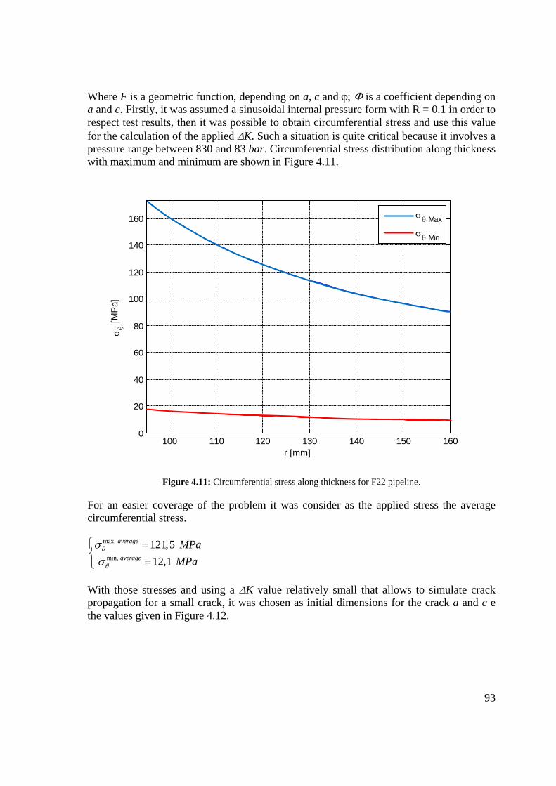
93

Where F is a geometric function, depending on a, c and ϕ; Φ is a coefficient depending on a and c. Firstly, it was assumed a sinusoidal internal pressure form with R = 0.1 in order to respect test results, then it was possible to obtain circumferential stress and use this value for the calculation of the applied ∆K. Such a situation is quite critical because it involves a pressure range between 830 and 83 bar. Circumferential stress distribution along thickness with maximum and minimum are shown in Figure 4.11.

Figure 4.11: Circumferential stress along thickness for F22 pipeline.

For an easier coverage of the problem it was consider as the applied stress the average circumferential stress.

max,

min,

121,512,1

average

average

MPaMPa

θ

θ

σσ

=

=

With those stresses and using a ∆K value relatively small that allows to simulate crack propagation for a small crack, it was chosen as initial dimensions for the crack a and c e the values given in Figure 4.12.

100 110 120 130 140 150 1600

20

40

60

80

100

120

140

160

Sigmaθ Vs raggio del condotto

r [mm]

σθ [M

Pa]

σθ Max

σθ Min

94

Figure 4.12: crack geometry.

In these conditions, initial ∆K is:

I,max

I,min

9,4328,489

0,943

K MPa mK MPa m

K MPa m

= ∆ ==

Those values were calculated in the point of maximum stress, therefore when ϕ = 90°. Only for illustrative purposes, initial ∆K for ϕ = 0° is given:

max,2

min,2

3,4593,114

0,346I c

I c

K MPa mK MPa m

K MPa m

= ∆ ==

Through data obtained from toughness tests it is possible to obtain Jc values for the F22 steel with and without hydrogen presence.

2_ _ 22

2_ _ 22

800 /150 /

c NoH F

c H F

J kJ mJ kJ m

==

Jc value without hydrogen is lower and taken with a safety factor compared to the real one for two reasons: it was taken as the average value between data obtained at -80°C and crack propagation during test was not enough long to obtain a Jc in respect with regulations. From these values it was possible to obtain KIc through the following equation.

2(1 )J EK

ν⋅

=−

4-11

95

And it was found:

,

,

425

184Ic NoH

Ic H

K MPa m

K MPa m

=

=

Rearranging equation and using as KI the known value of KIc and the maximum stress, it is possible to calculate the critical length of the crack. According to this procedure critical crack length is:

,

,

4060761

c NoH

c H

a mma mm

==

Results are extremely high and higher than the thickness of the pipeline that is equal to 65 mm, in this case there will be a leakage before break. On the other hand, considering the ductility of the material, plastic collapse should be taken into account. Calculations were performed according to BS regulations [49] (instructive derivations can be found in [24]). The reference stress is defined as it follows:

2 2 2 0.5

2

( 1) [( ( 1) ) 9 (1 ) ]3(1 )

b m m b m m mref

P k P P k P P ασα

+ − + + − + −=

− 4-12

If bending stresses are not considered and km = 1 is imposed, in absence of notches in the material, it is possible to apply the following equation:

2 2 2 0.5

2

[( ) 9 (1 ) ]3(1 )

m m mref

P P P ασα

− + − + −=

− 4-13

With:

( / )

1

a BBc

α =+

4-14

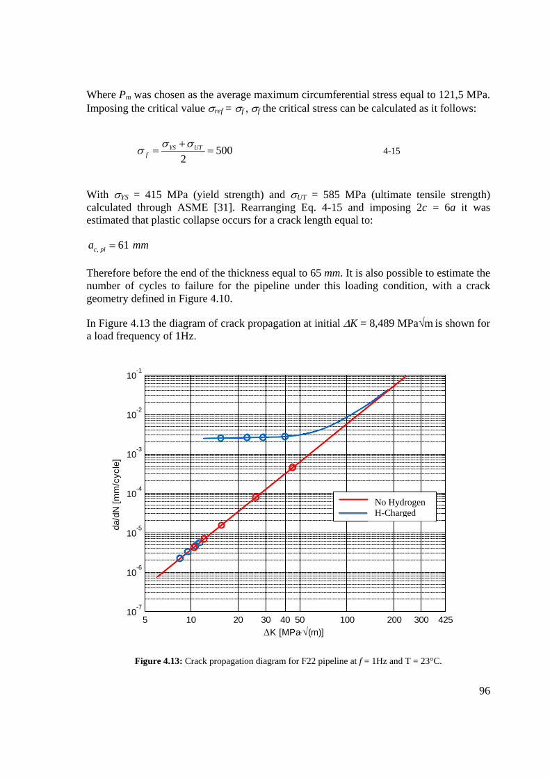
96

Where Pm was chosen as the average maximum circumferential stress equal to 121,5 MPa. Imposing the critical value σref = σf , σf the critical stress can be calculated as it follows:

5002

YS UTf

σ σσ += = 4-15

With σYS = 415 MPa (yield strength) and σUT = 585 MPa (ultimate tensile strength) calculated through ASME [31]. Rearranging Eq. 4-15 and imposing 2c = 6a it was estimated that plastic collapse occurs for a crack length equal to:

, 61c pla mm=

Therefore before the end of the thickness equal to 65 mm. It is also possible to estimate the number of cycles to failure for the pipeline under this loading condition, with a crack geometry defined in Figure 4.10.

In Figure 4.13 the diagram of crack propagation at initial ∆K = 8,489 MPa√m is shown for a load frequency of 1Hz.

Figure 4.13: Crack propagation diagram for F22 pipeline at f = 1Hz and T = 23°C.

5 10 20 30 40 50 100 200 300 42510

-7

10-6

10-5

10-4

10-3

10-2

10-1

Propagazione F22

∆K [MPa⋅√(m)]

da/d

N [m

m/c

ycle

]

Senza IdrogenoCon Idrogeno

No Hydrogen H-Charged

97

The model exposed previously was taken without considering the transient and starting hydrogen assisted cracking at 12K MPa m∆ = . This assumption was done considering data trend but it must be said that accurate measurements of ∆Kstart should be performed for a better understanding of the phenomena and a knowledge of hydrogen effect on all ∆K ranges.

It can be noted that for low ∆K hydrogen effect is not relevant and propagation occurs on the Paris line of the uncharged material. Once ∆K = 12 MPa√m is reached, hydrogen effect increases crack growth rate. When the crack length reaches a value of 61 mm plastic collapse occurs, this length is reached by the uncharged material in a number of cycles double compared to the hydrogen charged material:

,

, , 1 , 23

2185589989292

end NoH

end H Hz C

CyclesCycles °

==

In Figure 4.14 crack length as a function of the number of cycles is depicted for charged and uncharged material.

Figure 4.14: crack length as function of cycles at 1Hz and 23°C for F22 pipeline.

0 0.2 0.4 0.6 0.8 1 1.2 1.4 1.6 1.8 2

x 106

10

20

30

40

50

60Lunghezza di cricca Vs cicli

Lung

hezz

a di

cric

ca [m

m]

Cicli

Senza IdrogenoCon Idrogeno

No Hydrogen H-Charged

Cycles

Crac

k le

ngth

98

It is also possible to estimate graphically the crack growth shape as a function of the number of cycles, as shown in Figure 4.15 and Figure 4.16.

Figure 4.15: crack geometry as function of N of cycles for uncharged material at f = 1Hz and T = 23°C.

Figure 4.16: crack geometry as function of N of cycles for H-charged material at f=1Hz and T = 23°C.

If fatigue conditions took place with higher frequency, for example with frequency of 10 Hz, it would be possible to use the model to predict the number of cycles to failure, while keeping constant crack geometry and loading parameter; results are shown below:

, , 10 , 23 1123735end H Hz CCycles ° =

For obvious reasons, the number of cycles to failure for the material without hydrogen remains constant while varying frequency. In Figure 4.17 crack propagation diagram for F22 pipeline at 10 Hz and 23°C is shown while in Figure 4.18 the crack length as a function of the number of cycles either for hydrogen charged and uncharged is shown, until instability is reached.

-60 -40 -20 0 20 40 600

10

20

30

40

50

60

0

1.5e+006

2e+006

2.18559e+006Propagazione senza idrogeno

a [m

m]

c [mm]

-60 -40 -20 0 20 40 600

10

20

30

40

50

60

0

970000

975000

980000

989292Propagazione con idrogeno

a [m

m]

c [mm]

99

Figure 4.17: crack propagation diagram for a F22 pipeline at f=10Hz and T=23°C.

5 10 20 30 40 50 100 200 300 42510

-7

10-6

10-5

10-4

10-3

10-2

10-1 Propagazione F22

∆K [MPa⋅√(m)]

da/d

N [m

m/c

ycle

]

Senza IdrogenoCon Idrogeno

No Hydrogen H-Charged

100

Figure 4.18: crack length as function of cycles at 10Hz and 23°C for F22 pipeline.

It is also possible to vary the temperature and investigate, through the model, the number of cycles to failure in case of a temperature equal to -30°C and a loading frequency of 1 Hz; the number of cycles to failure are equal to:

, , 1 , 30 1042985end H Hz CCycles − ° =

In Figure 4.19 crack propagation diagram for the material with and without hydrogen is reported.

0 0.2 0.4 0.6 0.8 1 1.2 1.4 1.6 1.8 2

x 106

10

20

30

40

50

60Lunghezza di cricca Vs cicli

Lung

hezz

a di

cric

ca [m

m]

Cicli

Senza IdrogenoCon Idrogeno

No Hydrogen H-Charged

Crac

k le

ngth

Cr

ack

leng

th

Cycles

101

Figure 4.19: crack propagation diagram for a F22 pipeline at f=1Hz and T=-30°C.

4.4.2 Application of the model in a real case (X65 pipeline)

In this section the numerical analysis used for the F22 pipeline is carried out for X65 pipeline. Pressure ratio is kept constant with Pmax = 83MPa and Pmin = 8.3MPa, what changes are the circumferential stresses since pipeline dimensions are different: outer diameter in this case is equal to Do = 323 mm and the thickness is equal to t=46 mm. In these conditions circumferential stresses, maximum and minimum, are shown in Figure 4.20.

5 10 20 30 40 50 100 200 300 42510

-7

10-6

10-5

10-4

10-3

10-2

10-1

Propagazione F22

∆K [MPa⋅√(m)]

da/d

N [m

m/c

ycle

]

Senza IdrogenoCon Idrogeno

No Hydrogen H-Charged

102

Figure 4.20: Circumferential stress along thickness (X65 pipeline).

Also in this case the average circumferential stress is taken for the analysis:

max, ave

min,

215,321,5ave

MPaMPa

θ

θ

σσ

=

=

At ϕ = 90° and ϕ = 0° ∆K give the following values:

Imax

Imin

15,39513,856

1,539

K MPa mK MPa m

K MPa m

= ∆ ==

maxI, 2c

minI, 2c

71,19963,271

7,119

K MPa mK MPa m

K MPa m

= ∆ ==

From test data it is possible to obtain Jc for X65 steel either with hydrogen or without.

120 125 130 135 140 145 150 155 1600

50

100

150

200

250

r [mm]

σθ [M

Pa]

σθ Maxσθ Min

103

2, , 65

2, , 65

900 /90 /

c NoH X

c H X

J kJ mJ kJ m

==

Jc value without hydrogen is lower and taken with a safety factor compared to the real one for two reasons: it was taken as the average value between data obtained at -80°C and crack propagation during test was not enough long to obtain a Jc in respect with regulations. From this value, it was possible to obtain KIc through the following equation:

,

,

452

143Ic NoH

Ic H

K MPa m

K MPa m

=

=

Critical crack length is equal to:

,

,

1724173

c NoH

c H

a mma mm

==

Results are extremely high and over the thickness of the pipeline that is equal to 65 mm, in this case there will be a leakage before break. On the other hand, considering the ductility of the material, plastic collapse should be taken into account. As Pm value, upper average circumferential stress is taken that is equal to 215.3 MPa. Assuming that the critical value is reached, it is imposed that σref = σf where σf can be obtained as it follows:

489.52

YS UTf MPaσ σσ +

= =

With σYS = 415 MPa and σUT = 585 MPa calculated through API 5L [4]. Rearranging Eq. 4-15 and imposing 2c = 6a it was estimated that plastic collapse occurs for a crack length equal to:

, 39c pla mm=

Hence before the end of the thickness equal to 46 mm.

It is also possible to estimate the number of cycles to failure for the pipeline under this loading condition, with a crack geometry defined in Figure 4.12.

In Figure 4.21 the diagram of crack propagation at initial 13,86K MPa m∆ = is shown for a load frequency of 1Hz.

104

Figure 4.21: Crack propagation diagram for X65 pipeline at f=1Hz and T=23°C.

When the crack length has reached a value of 46 mm plastic collapse occurs, this length is reached by the uncharged material in a number of cycles double compared to the hydrogen charged material:

,

, , 1 , 23

26774314269

end NoH

end H Hz C

CyclesCycles °

==

In Figure 4.22, crack length as a function of number of cycles is shown for X65 pipeline.

5 10 20 30 40 50 100 200 300 45210

-7

10-6

10-5

10-4

10-3

10-2

10

∆K [MPa⋅√(m)]

da/d

N [m

m/c

ycle

]

Senza IdrogenoCon Idrogeno

No Hydrogen H-Charged

105

Figure 4.22: crack length as function of cycles at 1Hz and 23°C for X65 pipeline.

It is also possible to estimate graphically the crack growth shape as a function of the number of cycles, as shown in Figure 4.23 and Figure 4.24.

Figure 4.23: crack geometry as function of N of cycles for uncharged material at f=1Hz and T=23°C.

-40 -30 -20 -10 0 10 20 30 400

510

15

20

2530

35

0120000

200000

267743p g g

a [m

m]

c [mm]

0 0.5 1 1.5 2 2.5

x 105

5

10

15

20

25

30

35

Lunghezza di cricca Vs cicli

Lung

hezz

a di

cric

ca [m

m]

Cicli

Senza IdrogenoCon Idrogeno

Cycles

Crac

k le

ngth

No Hydrogen H-Charged

106

Figure 4.24: crack geometry as function of N of cycles for hydrogen charged material at f=1Hz and T=23°C.

If fatigue conditions took place with higher frequency, for example with frequency of 10 Hz, it would be possible to use the model to predict the number of cycles to failure, while keeping constant crack geometry and loading parameter; results are shown below:

, , 10 , 23 74389end H Hz CCycles ° =

For obvious reasons, the number of cycles to failure for the material without hydrogen remains constant while varying frequency. In Figure 4.25 crack propagation diagram for X65 pipeline at 10 Hz and 23°C is shown while in Figure 4.26 the crack length as a function of the number of cycles either for hydrogen charged and uncharged is shown at 10 Hz and 23°C.

-40 -30 -20 -10 0 10 20 30 400

5

10

15

20

25

30

35

0

3000

6000

14269p g g

a [m

m]

c [mm]

107

Figure 4.25: crack propagation diagram for a X65 pipeline at f=10Hz and T=23°C.

Figure 4.26: crack length as function of cycles at 10Hz and 23°C for X65 pipeline.

5 10 20 30 40 50 100 200 300 45210

-7

10-6

10-5

10-4

10-3

10-2

10

∆K [MPa⋅√(m)]

da/d

N [m

m/c

ycle

]

Senza IdrogenoCon Idrogeno

0 0.5 1 1.5 2 2.5

x 105

5

10

15

20

25

30

35

Lunghezza di cricca Vs cicli

Lung

hezz

a di

cric

ca [m

m]

Cicli

Senza IdrogenoCon Idrogeno

No Hydrogen H-Charged

Crac

k le

ngth

Cycles

No Hydrogen H-Charged

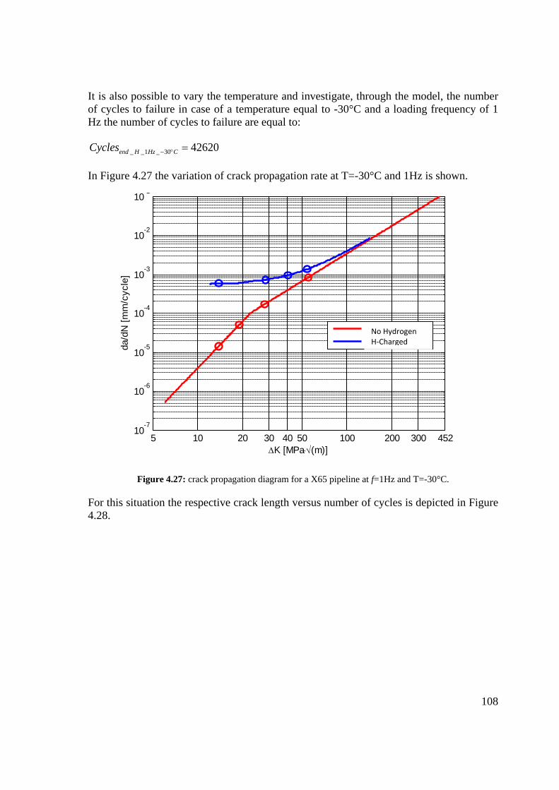
108

It is also possible to vary the temperature and investigate, through the model, the number of cycles to failure in case of a temperature equal to -30°C and a loading frequency of 1 Hz the number of cycles to failure are equal to:

_ _1 _ 30 42620end H Hz CCycles − ° =

In Figure 4.27 the variation of crack propagation rate at T=-30°C and 1Hz is shown.

Figure 4.27: crack propagation diagram for a X65 pipeline at f=1Hz and T=-30°C.

For this situation the respective crack length versus number of cycles is depicted in Figure 4.28.

5 10 20 30 40 50 100 200 300 45210

-7

10-6

10-5

10-4

10-3

10-2

101

∆K [MPa⋅√(m)]

da/d

N [m

m/c

ycle

]

Senza IdrogenoCon Idrogeno

No Hydrogen H-Charged

109

Figure 4.28: crack length as function of cycles at 1Hz and T=-30°C for X65 pipeline.

4.5 Remarks on models and its application

The superposition model and the thermal model proposed to interpret test data seem to fit satisfactorily test data, respect all the dependences between environmental conditions and material behavior and agree with previous investigations found in bibliography. It emerged that test data at low frequency and high temperature are better concentrated on the expected value and for this reason they should be used for interpolation. This fact can be owed to a larger enhancement of IHAC at low frequencies and higher temperatures that can be controlled better, on the other hand at lower temperatures and higher frequencies, parameters that were not taken into account can influence more the behavior. Another important fact that should be taken into account as a parameter, but for lack of tests was not possible to calculate, is the hydrogen content inside the lattice, from literature (reference [12]) it was found that by varying hydrogen content it is possible to have a better view of the phenomenon. It was also shown that, the model is easy to implement in real cases and can be applied to engineer consideration. The lack of the knowledge of ΔKth can be a limit when short cracks are considered (short-crack mechanics need a different approach), nevertheless the model is a powerful and relatively simple tool to calculate crack growth rates.

0 0.5 1 1.5 2 2.5

x 105

5

10

15

20

25

30

35

Lunghezza di cricca Vs cicli

Lung

hezz

a di

cric

ca [m

m]

Cicli

Senza IdrogenoCon Idrogeno

No Hydrogen H-Charged

Cycles

Crac

k le

ngth

110

5 SEM analysis on fracture surfaces

Special acknowledgement goes to Dipartimento di Chimica, Materiali e Ingegneria Chimica “G. Natta” of Politecnico di Milano that carried out and performed all SEM fractographs on specimens.

5.1 Introduction

Once fatigue crack growth and toughness tests were performed and plastic instability was reached, specimens have been opened by forced displacement. It was chosen to investigate the fracture surfaces via “scanning electron microscope” SEM both for the H-free specimens and for the charged specimen. Fractographs have been used in this work to verify the micro-mechanics of cracking and to compare the different mechanisms between the H-charged specimens and the H-free with model prediction, shown in chapter 4.

Attention has been focused on:

Striations in fatigue crack growth Different fracture surfaces Plastic deformation localization Blunting at crack tip Inclusions role Brittle fracture areas.

All this features were considered at different ΔK levels, H presence, temperature and type of test.

111

5.2 Fractographic analysis on uncharged specimens

5.2.1 Toughness specimens

In Figure 5.1 the fracture surface of H-free X65 steel CT specimen is shown at low magnification (200X), CT specimen was first tested for J-integral determination and then opened under forced displacement after plastic instability occurred. In the image, it is possible to recognize the steps of the test. First of all the specimen was fatigue pre-cracked to obtain a crack tip as sharp as possible. The following operation was testing as describe in section 3.4, with rising load, crack tip opening appeared to increase: this effect was due to crack tip radius increasing owing to plasticization. Figure 5.2 shows a magnification of tearing region, it can be observed a classical plastic pattern with void growth and microdimples. Also in this case the steel is behaving accordingly to its properties. Figure 5.3 shows a magnification of plastic instability region, fracture occurs by cleavage of grain planes, facets can be observed and reduced plastic work is performed by the material.

Figure 5.1: Fracture surface of a CT specimen X65 steel tested for J-integral determination shown at 200X. Fatigue precrack can be seen, blunting of the crack tip due to plasticity and tearing before instability, when

test was stopped. This figure can be referred to the load-displacement line shown in section 3.4. Fractographs carried out at Dipartimento di Chimica, Materiali e Ingegneria Chimica “G. Natta”.

112

Figure 5.2: Magnification of Figure 5.1 in the ductile “tearing” region. Large plasticity can be observed with micro-dimple structure [1000X]. Fractographs carried out at Dipartimento di Chimica, Materiali e Ingegneria Chimica “G. Natta”.

Figure 5.3: Magnification of Figure 5.1 in the plastic “instability” region. Cleavage around an inclusion can be observed [1500X]. Fractographs carried out at Dipartimento di Chimica, Materiali e Ingegneria Chimica “G. Natta”.

5.2.2 Fatigue crack growth specimens

In Figure 5.4, a zero magnification of the fracture surface of X65 steel H-free tested at f = 20 Hz and T = 23°C and used for Paris coefficients determination is reported.

In Figure 5.5, fracture surface of uncharged X65 steel shown in Figure 5.4, is given at magnification of 500X and 3000X. These fractographs show a typical ductile striations pattern in the direction of crack growth (from top to down) and in the left image it is possible to recognize perfectly rounded shape SCa inclusions (XRD analysis). Crack propagation appears regular and following grain orientation (the most favorable slip planes). In the left image, there are steps between fracture planes where there is a plastic deformation at the corners indicating plasticity of the materials in absence of constrains. Material appears to behave according to its known properties.

113

Figure 5.4: Opitcal image of the fracture surface of X65 steel H-free, investigated in Figure 5.5.

Figure 5.5: On the left side: fracture surface on X65 specimen used for Paris coefficients determination typical fatigue surface with few inclusions [500X]. On the right side: ductile striations on different slip planes in the direction of crack growth [3000X]. Fractographs carried out at Dipartimento di Chimica,

Materiali e Ingegneria Chimica “G. Natta”.

5.3 Fractographic analysis on H-charged specimens

5.3.1 Toughness specimen

In toughness tests in presence of hydrogen, the behavior of the material was different since there was a stable crack growth before instability; this indicates a reduction in plasticity of the material since no large crack blunting occurred but growth. Figure 5.6 and Figure 5.7 show the pattern of internal hydrogen assisted cracking that will be observed also in fatigue crack growth specimens. Fracture surface is marked by a mixed cell-like pattern: cells initiate from an inclusion and propagate in a quasi-cleavage way until a certain length; around the cell plastic work is performed since crests can be recognized. For this

114

reason the rupture is not completely brittle, even though plasticity loss is remarkable and can be noticed also from mechanical tests.

Figure 5.6: Fracture surface of X65 steel CT specimen H-charged in stable propagation. Cell-like fracture pattern can be recognize [100X]. Fractographs carried out at Dipartimento di Chimica, Materiali e Ingegneria Chimica “G. Natta”.

Figure 5.7: Magnification of Figure 5.6, cell-like structure is visible and fracture appears mixed: both cells and quasi-cleavage [1500X]. Inclusion in the center of the celli s present. Fractographs carried out at Dipartimento di Chimica, Materiali e Ingegneria Chimica “G. Natta”.

5.3.2 Fatigue crack propagation

Investigating fatigue crack growth fracture surfaces should take into account not only temperature and frequency but mainly the stress level ahead of the crack tip (given by the stress intensity factor ΔK) and the relative crack growth rate, in this way it is possible to obtain useful information about the model and the micro-mechanics of internal hydrogen assisted cracking.

Figure 5.8, Figure 5.9 and Figure 5.10 are given in order of increasing ΔK, the specimen in those pictures was tested in presence of hydrogen at f = 1Hz and T = 23°C. Figure 5.8 shows a magnification on X65 steel at low ΔK: in the da/dN-ΔK plot, this corresponds to a large scatter of data as shown in Figure 3.37 (orange dots); fractographs shows a crack growth with facets and steps-jumps in different directions and quasi-cleavage morphology. During mechanical testing it was difficult to explain data scattering at the beginning of tests and it was thought that transient could affect crack growth, from these fractographs it can be explained by the fact that crack growth is largely discontinuous since there are period in which there is no remarkable crack growth and periods in which jumps occur.

Figure 5.9 shows a magnification of the fracture surface at intermediate ΔK of a region were striations are visible. Surface appears to be brittle with small region of deformed material; striations follow the orientation of the grain and facets are clear. In Figure 3.37,

115

at intermediate ΔK, correspond to a less scattered data and the crack growth rate is higher than the uncharged material and it already reached the plateau level. Indeed, this is the maximum rate at which the crack will propagate throughout the test.

Finally at high ΔK, close to test-end, cell morphology shows up, as reported in Figure 5.10. It can be seen a magnification of a cell where the inclusion is placed in the center (indicating also low interface bonding), brittle surface around the inclusion and plastic work around the cell. Hence, at high ΔK, fracture feature of monotonic test is met. Cell fracture is not fully brittle and indicates a plastic response around the cell. This behavior appears to limit the rate of crack growth to increase over the plateau, since mechanical fatigue becomes dominant again.

Figure 5.8: fracture surface on X65 specimen tested at f = 10Hz and T = 23°C at low ΔK values (6 mm from machined notch). Brittle surface with cleavage feature and a ductile area in the middle [3000X] Fractographs carried out at Dipartimento di Chimica, Materiali e Ingegneria Chimica “G. Natta”.

Figure 5.9: fracture surface on X65 specimen tested at f = 10Hz and T = 23°C at medium ΔK values. Striations can be observed and cleavage planes with less plastic work [3000X] Fractographs carried out at Dipartimento di Chimica, Materiali e Ingegneria Chimica “G. Natta”.

116

Figure 5.10: fracture surface on X65 specimen tested at f = 10Hz and T = 23°C at high ΔK values. Particular of a cell [29900X] Fractographs carried out at Dipartimento di Chimica, Materiali e Ingegneria

Chimica “G. Natta”.

5.4 Considerations on fracture surfaces and predicting model

Fractographs conducted on CT specimen tested for J-integral and fatigue crack growth gave interesting results. It appeared that the main difference between H-charged and uncharged specimens is the presence of facet-like feature at low stress level indicating reduced plasticity and cell-like feature at high stress level indication both localization of stresses at inclusions giving a quasi-cleavage morphology and a plastic response around the cell indicating that the material has still some plastic reserve available. Fractographs also shown that both brittle and plastic features are present in H-charged fracture surface indicating that the superposition model has a physical justification. Indeed it appeared that fatigue crack growth (FCG) is enhanced by hydrogen but there is always a constrain owing to plastic reserve in the material; as an evidence of this behavior, in final steps of FCG both monotonic and fatigue fracture mechanisms appeared to be the same. It is not easy to assess the extract role of hydrogen in cracking, nevertheless an interesting comparison in void nucleation and growth was given by Murakami [12] and depicted in Figure 5.11. Referring to HE models given in chapter 2, hydrogen interacts with void nucleation and growth by segregating around the inclusion where both stresses and dislocation concentration are higher and affecting the behavior of the material, reducing its ability to flow. Feature in Figure 5.11 resembles cell morphology and can be a good explanation of the phenomenon. Figure 5.12 shows a schematic of striation formation in presence and without hydrogen. Firstly, it can be observed that hydrogen is segregated at crack tip where hydrostatic stresses are high (as explained in chapter 2), concentration ahead of the crack is then increased respect to the bulk material. Secondly, hydrogen effect lies in reducing plasticity by reducing crack blunting as it can be seen by comparing the two cases. In this way, hydrogen enhances the crack growth since Δa is larger in hydrogen

117

presence than in H-free material. Hydrogen, by lowering plasticity of the material, reduces also striations formation: indeed, if Figure 5.5 is compared with Figure 5.9, it can be observed that striations in presence of hydrogen are less clear and crests are less marked.

Figure 5.11: Schematic illustration of nucleation, growth and coalescence of voids with and without hydrogen in metals [12].

118

Figure 5.12: Crack tip opening and striation formation mechanism in fatigue: (a) no hydrogen effect, (b) hydrogen effect, (c) schematic effect of thick plastic zone wake produced at crack tip under no hydrogen and

(d) schematic image of shallow plastic zone wake produced at a crack under hydrogen effect [12].

Another feature that was observed clearly in FCG was the facet-like morphology, in this case and according to da/dN-ΔK plot a large scatter of data was observed, indeed it is not easy to assess the reason of this scattering but of course the jump-like growth is probable to be responsible. Facets were found between plastic deformed material.

In conclusion, it is not easy to assess surely by fractographic analysis the mechanism governing the cracking, nevertheless a main feature emerges: cracking in presence of hydrogen proceeds both by brittle and ductile mode and propagation occurs by jumps of brittle material that are constrained by plastic reserve. This fact underlines the diffusion dependence of the phenomenon and justifies the plateau rate.

The predicting model, shown in chapter 4, appears to be in accordance with micro observations. Nevertheless is should always be kept in mind that too daring conclusions

119

are far to be drawn from few fractographic investigation and this chapter is useful for a first insight on micromechanics of IHAC.

120

Conclusions

In this thesis work the fracture-mechanical properties of two steels widely used in oil pipeline have been investigated in a wide temperature range and with and without the presence of hydrogen in the lattice. Investigation was possible thanks to an electrochemical non-hazardous technique developed at Dipartimento di chimica, materiali e ingegneria chimica G. “Natta” able to effectively charge the specimens with a hydrogen content of around 0,9-1,3 ppm. From fatigue crack growth test data it was possible to propose a model able to predict the behavior of the two steels as a function of test variables and it was applied to real case. Finally thanks to FEM fractographs it was possible to give a better understanding of the phenomena.

From first two chapters, powerful tools and literature data were reported in order to clarify the phenomenon:

“sour” environments enhances the penetration of atomic hydrogen in the metal lattice

Hydrogen in the lattice is able to worsen fracture properties of steel in particular of condition of sustained loads and fatigue crack growth by reducing plasticity

A practical definition of HE was given and all its features (diffusion, kinetics and stress state) have been quantified and showed

Micromechanical models of hydrogen embrittlement were given.

In third chapter, dealing with experimental procedures and data:

A mechanical testing procedure was shown for hydrogen charged specimens in order to obtain useful mechanical parameters such as: Charpy impact energy, toughness and fatigue crack growth rate varying test temperature from room temperature until a value of T = - 120°C, without any remarkable hydrogen loss in the material

121

Mechanical tests on charged hydrogen showed a drastic change in properties respect to the uncharged one

Hydrogen effect, as shown in previous chapters, was remarkably enhanced by long time tests such as J-integral: the characteristic toughness value, Jq, shows a loss in mechanical performances up to 8 times bigger if compared to the uncharged one. In particular the material loses the ability to plasticize under high loads and stresses and its behavior shifts to those of medium tough steels.

Hydrogen effect is not temperature dependent and Jq values, experimentally obtained from charged specimens, are very similar while varying test temperature: for F22 steel Jq≈150 KJ/m2 and for X65 steel Jq≈90 KJ/m2.

Even though steels are sensible to hydrogen J values remain high.

Fatigue crack propagation tests were performed on uncharged specimens to establish Paris law parameters: F22 shows a typical behavior of steels with an exponent m≈3 and temperature influence was not observed; X65 shows a different behavior with a slope change in the II region around ΔK≈23 MPa√m. For ΔK<23 MPa√m m≈3.9 and for ΔK>23 MPa√m m≈2.4

Fatigue crack propagation tests were carried out on hydrogen charged specimens. Hydrogen effect was clearly observed and influenced by load frequency and temperature. The most important parameter is the time in which hydrogen is at crack tip: low frequencies allow the hydrogen to migrate at the crack tip; as a consequence hydrogen embrittlement effect and crack growth rate are enhanced. Low temperature affect the hydrogen diffusion coefficient in the steel: low temperatures reduce the mobility of hydrogen in the lattice, reducing the embrittling effect due to hydrogen

A model able to predict the behaviour of the steels that takes into account experimental variables have been proposed:

Crack growth rate is the sum of two contributions: one named “mechanical” that depends on applied loads and a second due to hydrogen effect. When crack growth rate increases, the “mechanical” contribution prevails because hydrogen atoms do not have enough time to accumulate at the crack tip: as a consequence crack growth rate is no longer hydrogen dependent.

A predicting model of fatigue crack growth rate as function of temperature and frequency was proposed. The model is based on the superposition of baseline fatigue crack growth (mechanical) and a sustained crack growth owing to internal hydrogen, this rate was found to be proportional to the square root of diffusivity and hydrogen content

122

Model gave good results and fitted satisfactory the data

Model was applied to real cases showing simplicity in application and usefulness

Finally a fractographic analysis was carried out onto fracture surfaces of C(T) specimens used for J-integral and crack growth determination. Fractographs showed that in presence of hydrogen there is a clear change in fracture morphology and that plasticity is reduced. Moreover experimental evidences to theory reasoning shown in chapter 2 were found.

Fracture morphology in absence of hydrogen is typical of the class of the steels with dimples in the stable propagation and quasi-cleavage morphology in unstable propagation

In presence of hydrogen fracture morphology presents facets and cell-like structure indicating a reduction of plasticity due to hydrogen, nevertheless a partial plastic reserve is available for the material, in fact around facets and cells plasticized zones have been identified

Viable micro-mechanisms have been proposed according to bibliography and they seem to interpret correctly the phenomenon

Fractographs evidenced that superposition model is justified since both mechanisms have been found (striations and hydrogen embrittled morphology

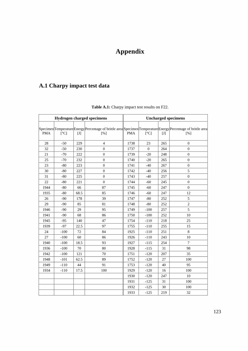
123

Appendix

A.1 Charpy impact test data

Table A.1: Charpy impact test results on F22.

Hydrogen charged specimens Uncharged specimens

Specimen PMA

Temperature [°C]

Energy [J]

Percentage of brittle area [%] Specimen

PMA Temperature

[°C] Energy

[J] Percentage of brittle area

[%]

28 -50 229 4 1738 23 265 0 32 -50 230 0 1737 0 264 0 21 -70 222 0 1739 -20 248 0 25 -70 232 0 1740 -20 265 0 23 -80 223 0 1741 -40 267 0 30 -80 227 0 1742 -40 256 5 31 -80 225 0 1743 -40 257 0 22 -80 221 0 1744 -60 245 0

1944 -80 66 87 1745 -60 247 0 1935 -80 68.5 85 1746 -60 247 12 26 -90 178 39 1747 -80 252 5 29 -90 85 81 1748 -80 252 2

1946 -90 29 95 1749 -100 257 5 1941 -90 68 86 1750 -100 252 10 1945 -95 140 47 1754 -110 218 25 1939 -97 22.5 97 1755 -110 255 15 24 -100 72 84 1925 -110 251 8 27 -100 60 86 1926 -110 243 10

1940 -100 18.5 93 1927 -115 254 7 1936 -100 70 80 1928 -115 31 98 1942 -100 121 70 1751 -120 207 35 1948 -101 62.5 89 1752 -120 27 100 1949 -110 44 91 1753 -120 40 95 1934 -110 17.5 100 1929 -120 16 100

1930 -120 247 10 1931 -125 31 100 1932 -125 30 100 1933 -125 219 32

124

Table A.2: Charpy impact test results on X65.

Hydrogen charged specimens Uncharged specimens

Specimen PMA

Temperature [°C]

Energy [J]

Percentage of brittle area [%] Specimen

PMA Temperature

[°C] Energy

[J] Percentage of brittle area

[%]

1976 23 207 0 1438 23 241 0 1952 23 222 0 1449 23 234 0

7 -3 156 37 1436 23 235 0 13 -3 159 37 1974 -20 174 37 20 -20 153 46 1980 -20 244.5 0 3 -20 222 0 1995 -40 227 14 2 -40 155 53 1983 -40 238 11 17 -40 182 38 1989 -60 156 50

1979 -50 184 47 1992 -60 162.5 50 8 -50 189 35 1961 -60 187 39 18 -50 164 49 1967 -80 68 86

1991 -60 181 36 1962 -80 120 73 1981 -60 172 45 1960 -80 145.5 70 1984 -60 161 51 1966 -90 88.5 83 10 -60 144 32 1959 -90 116 76 12 -60 229 67 1956 -90 160 47

1969 -70 162 56 1957 -100 29 100 1993 -70 100 79 1963 -100 103 78 1978 -70 152 58 1951 -100 17.5 100 1987 -70 159 55 1950 -100 25 100

6 -70 170 51 1964 -105 2 100 16 -70 181 44 1955 -105 8.5 100

1971 -80 138 61 1970 -80 33 99 1975 -80 137 64 1996 -80 114 73 1958 -80 160 58 1977 -80 87 81

9 -80 148 57 19 -80 154 59

1994 -90 45 94 1990 -90 110 77 1973 -90 81 86 1954 -90 12.5 100 1953 -90 20.5 100 1988 -90 120 73

4 -90 16 100 11 -90 169 46

1985 -90 28 95 1972 -100 11 100 1986 -100 8 100

125

5 -100 161 30 15 -100 21 97 14 -110 6 100 1 -110 10 100

A.2 Toughness test data

Table A.3: Toughness test results on F22 steel. Colors indicating H-charging as shown in Figure 3.22.

Specimen

Temperature [°C]

Final propagation

J [kJ/m2]

Jel [kJ/m2]

Jpl [kJ/m2]

CTOD [mm]

CTODel [mm]

CTODpl [mm]

PMA2073sH -90 STABLE 176.1 65.4 109.8 0.165 0.070 0.095 PMA2072sH -80 STABLE 228.9 51.5 170.5 0.208 0.055 0.153 PMA2071sH -70 STABLE 166.4 63.7 102.0 0.156 0.068 0.087 PMA1766sH -60 STABLE 115.2 37.2 77.3 0.108 0.040 0.068 PMA2070sH -50 STABLE 131.0 55.8 74.9 0.123 0.060 0.063 PMA2076sH -40 STABLE 192.4 68.4 120.1 0.177 0.073 0.104 PMA2082sH -40 STABLE 185.4 59.1 125.5 0.173 0.063 0.110 PMA1770sH -30 STABLE 120.7 36.2 83.8 0.113 0.039 0.074 PMA2091sH -10 STABLE 190.7 57.7 131.8 0.178 0.062 0.116 PMA2078sH -10 UNSTABLE 137.3 51.0 86.3 0.129 0.054 0.074 PMA2074sH 23 STABLE 212.3 58.5 152.5 0.198 0.063 0.136

PMA2087s -120 UNSTABLE 360.1 99.8 263.7 0.341 0.107 0.235 PMA2094s -110 UNSTABLE 491.7 80.7 411.2 0.462 0.086 0.376 PMA2092s -100 STABLE 898.7 88.7 801.7 0.836 0.095 0.741 PMA1775 -80 STABLE 945.0 91.3 850.3 0.884 0.097 0.786 PMA1762 -80 STABLE 649.5 68.6 579.4 0.608 0.073 0.535

PMA2079sH -40 STABLE 416.7 65.3 347.1 0.387 0.070 0.317 PMA2089sH -40 STABLE 217.6 27.8 188.0 0.203 0.030 0.173 PMA2086sH -70 STABLE 251.7 27.9 221.8 0.234 0.030 0.205 PMA2085sH -70 STABLE 177.6 27.4 149.0 0.166 0.029 0.136

126

Table A.4: Toughness test results on F22 steel. Colors indicating H-charging as shown in Figure 3.23.

Specimen

Temperature [°C]

Final propagation

J [kJ/m2]

Jel [kJ/m2]

Jpl [kJ/m2]

CTOD [mm]

CTODel [mm]

CTODpl [mm]

PMA2106sH -80 UNSTABLE 131.3 67.1 64.2 0.120 0.066 0.054 PMA2102sH -70 UNSTABLE 107.8 64.1 43.8 0.099 0.063 0.036 PMA2119sH -70 UNSTABLE 69.3 50.4 19.0 0.063 0.049 0.014 PMA2118sH -60 UNSTABLE 111.9 66.8 45.1 0.102 0.065 0.037 PMA2109sH -60 UNSTABLE 111.4 64.1 47.3 0.102 0.063 0.039 PMA2110sH -50 UNSTABLE 96.3 50.9 45.4 0.088 0.050 0.038 PMA2111sH -50 UNSTABLE 72.1 54.8 17.3 0.066 0.054 0.012 PMA2100sH -40 UNSTABLE 84.9 54.1 30.8 0.078 0.053 0.025 PMA2126sH -40 STABLE 62.2 32.6 29.6 0.057 0.032 0.025 PMA2116sH 23 STABLE 142.8 55.1 87.3 0.13 0.054 0.076 PMA2117sH 23 STABLE 151.7 62.2 88.9 0.14 0.061 0.077

PMA2112s -100 UNSTABLE 154.5 66.4 88.2 0.141 0.065 0.076 PMA2107s -100 UNSTABLE 316.0 78.7 237.3 0.289 0.077 0.212 PMA2114s -90 UNSTABLE 461.2 80.3 380.9 0.422 0.078 0.343 PMA2113s -90 UNSTABLE 75.8 53.0 22.8 0.069 0.052 0.017 PMA2125s -80 STABLE 825.4 81.3 744.2 0.755 0.079 0.675 PMA2097s -80 UNSTABLE 663.1 90.2 572.8 0.606 0.088 0.518 PMA2096s -70 STABLE 921.7 92.0 829.8 0.843 0.090 0.753 PMA2098s -70 STABLE 841.7 82.7 758.9 0.770 0.081 0.689

127

Bibliography

[1] - Guidelines on Materials Requirements for Carbon and Low Alloy Steels for H2S-Containing Environments in Oil and Gas Production (3rd Edition) - European Federation of Corrosion Publications, Maney Publishing, 2009.

[2] Govindan Namboodhiri T.K., Tiruvalla - Hydrogen Damage of Metallic Materials - Kerala, India, 2008. URL: http://knol.google.com/k/hydrogen-damage-of-metallic-materials#

[3] Bræstrup M. W., Andersen J. B. - Design and installation of marine pipelines – Wiley Blackwell, 2005

[4] Mostert R. - Low Temperature Hydrogen Damage Assessment in the Gas and Refining Industries - Middle East Nondestructive Testing Conference & Exhibition, 27-30 Nov 2005 Bahrain, Manama.

[5] Möser M. and Schmidt V. - Fractography and mechanisms of hydrogen cracking, the fisheye concept - In S. R. Valluri, D. H. R. Taplin, P. Rama Rao, J. F. Knott and R. Dubey (eds.), Advances in Fracture Research, Proc. 6th Int. Conf. on Fracture, New Delhi, 1984, Vol. 4, Pergamon, Oxford, 1984, pp. 2459 – 2466.

[6] - Materials for use in H2S-containing environments in oil and gas production - ANSI/NACE MR0175-2009, petroleum and natural gas industries, Parts 1, 2, and 3 (Identical to ISO 15156-1:2009, 15156-2:2009, and 15156-3:2009).

[7] Gangloff R. P. - Hydrogen assisted cracking of high strength alloys - University of Virginia Charlottesville, VA 22904-4252 USA.

[8] Troiano A.R., Gibala R., Hehemann R. F. - Hydrogen embrittlement and stress corrosion cracking: a Troiano Festschrift- American Society for Metals, 1984.

[9] Troiano A.R. - Campbell Memorial Lecture - Trans. ASM, Vol. 52, 1960, p. 54.

[10] Capelle J., Gilgert J., Pluvinage G. - Hydrogen effect on fatigue and fracture of pipelines - Paper presented at the conference ICMFM XIII, 2006.

[11] Dong C.F, Liu Z.Y., Li X.G., Cheng Y.F. - Effects of hydrogen-charging on the susceptibility of X100 pipeline steel to hydrogen-induced cracking - International Journal of Hydrogen Energy, Vol. 34, Issue 24, 2009, Pages 9879-9884.

[12] Murakami Y. and Matsuoka S. - Effect of hydrogen on fatigue crack growth of metals - Engineering Fracture Mechanics, Vol. 77, Issue 11, 2010, Pages 1926-1940.

128

[13] Grabke H. J., Riecke E. - Absorption and diffusion of hydrogen in steels - Materiali in tehnologije, Vol. 34, 2000, p. 331-341.

[14] Woodtli J., Kieselbach R. - Damage due to Hydrogen Embrittlement and Stress Corrosion Cracking - Engineering Failure Analysis, Vol. 7, 2000, p. 427-450

[15] Ragone D. V. - Thermodynamics of Materials Volume II - John Wiley and Sons, 1995.

[16] XU J., SUN X. - Hydrogen permeation and diffusion in low-carbon steels and 16 Mn steel - Journal of Materials Science Technology 10, 1994, p. 92-96.

[17] Darken L. S. and Smith R. P. - Behavior of hydrogen in steel during and after immersion in acid - Corrosion 5, 1949, p. 1-16.

[18] McCright R. D. - Effects of environmental species and metallurgical structure on the hydrogen entry into steel - Stress corrosion cracking and hydrogen embrittlement of iron base alloys - NACE, Vol. 5, 1977, p. 306-325.

[19] Kumnick A. J. and Jonhson H. H. - Deep trapping state for hydrogen in deformed iron - Acta Metallurgica, Vol. 28, 1980, p. 33-39.

[20] Oriani R.A. - The diffusion and trapping of hydrogen in steel - Acta Metallurgica, Vol. 18, Issue 1, 1970, p. 147-157.

[21] McNabb A. and Foster P. K. - - Trans. TMS-AIME, vol. 227, 1963, p. 618.

[22] Kirchheim R. - Revisiting hydrogen embrittlement models and hydrogen-induced homogeneous nucleation of dislocations - scripta materialia, Vol. 62, 2009, p. 67-70.

[23] Dadfarnia, M., B. P. Somerday, P. Sofronis, I. M. Robertson, and D. Stalheim, - Interaction of Hydrogen Transport and Material Elastoplasticity in Pipeline Steels - Journal of Pressure Vessel and Technology, Vol.131, , 2009, p. 1-13.

[24] Vergani L. - Meccanica dei materiali - McGraw-Hill Companies, 2006.

[25] Janssen M., Zuidema J., Wanhill R.J.H. - Fracture mechanics, 2nd edition - VSSD, 2006.

[26] Anderson T.L. - Fracture mechanics: fundamentals and applications - Taylor & Francis, 2005.

[27] Oriani R. A. and Josephic P. H., Acta Metall., Vol. 22, 1974, p. 1065.

[28] Lynch S. P. – Progress towards understanding mechanisms of hydrogen embrittlement and stress corrosion cracking – Corrosion NACE, 2007.

[29] Sobotka J.C., Dodds Jr. R.H., Sofronis P. - Effects of hydrogen on steady, ductile crack growth: Computational studies - International Journal of Solids and Structures, Vol. 46, Issues 22-23, 2009, p. 4095-4106.

[30] Lazzari L., Fumagalli G., Bolzoni F., Re G., Stranieri A. - Carica di idrogeno per via elettrochimica su acciai (Tesi di laurea di Stranieri A.) - Politecnico di Milano, 2010.

129

[31] - Specification for forged or rolled alloy-steel, pipe flanges, forged fittings and valves and parts for high-temperature service - ASME BPVC Section II, 2004, SA-182.

[32] ASTM E 8/E 8M-08 - Standard test methods for tension testing of metallic materials.

[33] ASTM E 23-07 - Standard test methods for notched bar Impact testing of metallic materials.

[34] ASTM E 1829-08 – Standard test methods for measurements of fracture toughness.

[35] - Petroleum and natural gas industries - Steel pipe for pipeline transportation systems - Second Edition - ISO 3183. International Organization for Standardization, 2007.

[36] - Specification for Line Pipe - Forty-third edition API, Specification 5L, 2004.

[37] - Metallic materials, Charpy pendulum, impact test - ISO 148. International Organization for Standardization, 2009.

[38] - Standard Test Method for Measurement of Fracture Toughness - ASTM International, E 1820. 2009.

[39] Green G., Knott F. J. - Effects of Side Grooves on Initiation and Propagation of Ductile Fracture - Met. Technol. 2, Vol. 9, 1975, p. 422-427.

[40] Yasufumi I., Tomokazu M. - Effect of Side Grooves for Three-point Bending Fracture Toughness Specimens: Three-dimensional Elastic-plastic Finite Element Analysis - Bulletin of JSME 27, Vol. 227, 1984, p. 909-916.

[41] Sciuccati A., - L’importanza dei side-grooves per lo stato di sforzo in provini per meccanica della frattura - AIAS XXXIX Convegno Nazionale, Maratea, 2010.

[42] - ASTM International, E 647-08 - Standard Test Method for Measurement of Fatigue Crack Growth Rates.

[43] Kanezaki T., Narazaki C., Mine Y., Matsuoka S., Murakami Y. - Effects of hydrogen on fatigue crack growth behavior of austenitic stainless steels - International Journal of Hydrogen Energy, Vol. 33, 2008, p. 2604 - 2619.

[44] Wei R.P., Ming Gao, - Reconsideration of the superposition model for environmentally assisted fatigue crack growth - Scripta Metallurgica, Vol. 17, 1983, p. 959 - 962.

[45] Knop M., Heath J., Sterjovski Z., Lynch S.P. - Effects of cycle frequency on corrosion-fatigue crack growth in cathodically protected high-strength steels - Procedia Engineering 2, 2010, 1243–1252

[46] Oriani R.A. - The Physical and Metallurgical Aspects of Hydrogen in Metals - ICCF4, Fourth International Conference on Cold Fusion, 1993

130

[47] Nelson H. G. and Williams D. P. , Proc. Intl. Conf. on Stress Corrosion Cracking and Hydrogen Embrittlement of Iron Based Alloys - NACE, Huston, 1997, p. 390-404.

[48] Van Leeuwen H.P. - Plateau velocity of SCC in high strength steels A quantitative treatment - NACE Corrosion 31, Vol.2, 1975, p. 42–50.

[49] - Guide on methods for assessing the acceptability of flaws in fusion welded structures - British Standard, BS 7910, 1999.