INVESTIGATION OF THE APPLICATION OF HYDROPHOBIC AND

HYDROPHILIC PROPERTY IN HYDRODYNAMICS OF NAVAL ENGINEERING

Pedro de Mesquita Soares Campos

Projeto de Graduação apresentado ao Curso de Engenharia Naval e Oceânica da Escola Politécnica, Universidade Federal do Rio de Janeiro, como parte dos requisitos necessários à obtenção do título de Engenheiro Naval e Oceânico.

Orientador: Antonio Carlos Fernandes

Rio de Janeiro Fevereiro 2015

iii

INVESTIGAÇÃO DA APLICAÇÃO DE PROPRIEDADE HIDROFÓBICA E

HIDROFÍLICA EM HIDRODINÂMICA DA ENGENHARIA NAVAL E OCEÂNICA.

Pedro de Mesquita Soares Campos

PROJETO DE GRADUAÇÃO SUBMETIDO AO CORPO DOCENTE DO CURSO

DE ENGENHARIA NAVAL E OCEÂNICA DA ESCOLA POLITÉCNICA DA

UNIVERSIDADE FEDERAL DO RIO DE JANEIRO COMO PARTE DOS

REQUISITOS NECESSÁRIOS PARA A OBTENÇÃO DO GRAU DE

ENGENHEIRO NAVAL.

Examinado por:

_____________________________________________

Ph. D. Antônio Carlos Fernandes

_____________________________________________

Ph. D. Juan Bautista Villa Wanderley

_____________________________________________

D. Severino Fonseca da Silva Neto

RIO DE JANEIRO, RJ – BRASIL.

FEVEREIRO DE 2015

iv

Campos, Pedro de Mesquita Soares

Investigation of the application of hydrophobic and hydrophilic property in hydrodynamics of Naval Engineering / Pedro de Mesquita Soares Campos. – Rio de Janeiro: UFRJ/ Escola Politécnica, 2015.

XII, 51 p.: il.; 29,7 cm.

Orientador: Antônio Carlos Fernandes

Projeto de Graduação – UFRJ/ Escola Politécnica/ Curso de Engenharia Naval e Oceânica, 2015.

Referências Bibliográficas: p. 38-40.

1. Solid-Fluid Interaction. 2. Superhidrophobic and Superhydrophilic property. 3. Hydrodynamic Efficiency. 4. Vortex Induced Vibrations. I. Carlos Fernandes, Antônio. II. Universidade Federal do Rio de Janeiro, Escola Politécnica, Curso de Engenharia Navel e Oceânica. III. Investigação da aplicação de propriedades hidrofóbicas e hidrofílicas na hidrodinâmica de engenharia naval.

v

DED IC AT IO N

I dedicate this work as a fulfillment of Naval Architect and

Marine Engineer to the ones mostly present and dearest in

my life:

Mother Ana Claudia de Mesquita Soares and father Marcio

Benício Campos.

Dedicate to the person that always had an admiration for

the naval engineering and had an influence on my career:

Grandpa, Jhuan Hasmussem Thjesem

Dedicate to the person who always remembers me despite

the distance:

Grand grandpa, Arilo

Dedicate to both my grandmas for their love and pray.

Grandmas, Ana and Therezinha

Finally, I dedicate to those that I could not share with, but

has always been by my side:

Grandpa Orbene and Grandpa Marcio

vi

AC KN O WLE D GM EN T

Thanks God, for helping me through the presence of those

people in my life to overcome the challenges and

difficulties in this journey:

Professor Antônio Carlos Fernandes and Mohammad

Mobasher Amini for being my advisors and friends and the

LOC’s staff friends Luiz Antônio, Anderson Araujo, Igor

Santos and Werner Barros.

My english teacher, friend and beloved sibling Joseph

William Aitken for improving the text work.

TCE Shipyard co-workers Rodrigo Ferro, Pedro Henrique,

Marcelo Pimentel, Rafael Paisano , Alexandre Kopler, Luis

Sergio, Juliana Madeira and of course Juberto Pimentel

for given me at the time the best work environment anyone

could dream of.

All my childhood friends: King & Lolo, Dogo, Esquilo,

Guigão, Phil, Daninho, Caputo, Madu, Madimbu, Romano,

Índio, Glicose, Nana, Leleka and Goose for supporting me.

Princess Mabel Cremonini (bebel) for being the best friend

and companion specially in the hard time.

All my family “Mesquita”, Campos”, and especially all my

cousins.

My grandmas Terezinha and Ana.

My grandpas Marcio, Orbene and Jhuan

At least, but most important thanks to:

My father Marcio Benício Campos and mother Ana

Claudia de Mesquita Soares. Love you so much!

vii

Resumo do Projeto de Graduação apresentado à Escola Politécnca/ UFRJ como parte

dos requisitos necessários para a obtenção do grau de Engenheiro Naval.

INVESTIGAÇÃO DA IMPLICÂNCIA DA PROPRIEDADE HIDROFÓBICA E

HIDROFÍLICA EM HIDRODINÂMICA DA ENGENHARIA NAVAL.

Pedro de Mesquita Soares Campos

Fevereiro/2015

Orientador: Antônio Carlos Fernandes

Curso: Engenharia Naval e Oceânica

Este trabalho teoriza uma utilização conjunta de propriedades superhidrofóbicas e

superhidrofílicas, busca analisar a implicância das forças de adesão entre fluido e

substrato na dinâmica do escoamento e investiga os efeitos em um ensaio de vibrações

induzidas por vórtices.

Inicialmente o princípio do acabamento e a física que regem o estudo dessa proposta são

explicados e posteriormente uma investigação experimental da VIV em um grau de

liberdade foi conduzida com um modelo cilíndrico superhidrofóbico, superhidrofílico e

de superfície lisa comparando os resultados.

viii

Abstract of Graduation Project presented to COPPE / UFRJ as a partial fulfillment of the requirements for the degree of Marine Engineer and Naval Architect.

INVESTIGATION OF THE APPLICATIONS OF HYDROPHOBIC AND HYDROPHILIC

PROPERTY IN HYDRODYNAMICS OF NAVAL ENGINEERING

Pedro de Mesquita Soares Campos

Fevereiro/2015

Adviser: Antonio Carlos Fernandes

Department: Marine Engineering and Naval Architecture

This work theoretically proposes and studies the use of superhydrophobic and

superhydrophilic properties, aims to find the influence of interaction forces between

fluid and substrate on dynamics of the flow and investigates the effects on a vortex

induced vibrations experiment.

Initially the principle and physics that permeates the proposition is explained and

further an experimental 1DOF (one degree of freedom) VIV investigation with smooth,

superhydrophobic, superhydrophilic circular cylinders was set to compare the results.

ix

SUMMARY

Dedication ................................................................................................................................................... vi

Acknowledgment ........................................................................................................................................ vii

1. Introduction ......................................................................................................................................... 1

1.1. The Water as Continuum Medium .............................................................................................. 2

1.2. Fluid-Solid Interaction ................................................................................................................ 3

1.3. Superhydrophobicity and Superhydrophilicity ........................................................................... 4

2. Superhydrophobicity and Influence on Friction, vortex generation and Vortex Induced Vibrations. . 7

3. Questioning the Lack of Fluid-Solid Forces ...................................................................................... 13

4. The Proposition Explained................................................................................................................. 15

4.1. Physics and Mathematics .......................................................................................................... 17

5. About The Experiments ..................................................................................................................... 21

5.1. Vortex Induced Vibrations ........................................................................................................ 21

5.2. One degree of Freedom – VIV Experiment .............................................................................. 22

5.3. The Lab ..................................................................................................................................... 27

5.4. Experimental Set Up ................................................................................................................. 28

5.5. Results ....................................................................................................................................... 29

6. Conclusion ......................................................................................................................................... 34

7. References ......................................................................................................................................... 35

8. Annex I .............................................................................................................................................. 38

9. Annex II ............................................................................................................................................. 41

9.1. Decay graphs ............................................................................................................................. 41

9.2. Peak graphs and Exponential approximation ............................................................................ 44

9.3. Amplitude ratio Graphs ............................................................................................................. 47

9.4. Frequency ratio Graphs ............................................................................................................. 48

9.5. Velocity table ............................................................................................................................ 49

x

INDEX OF FIGURES

Figure 1 – Isolated water molecule in liquid state [1]. ________________________________________ 2 Figure 2- Schematics of molecules at the surface and the resultant force inwards [4] _______________ 3 Figure 4 - List of materials and their critical surface tension [1]. _______________________________ 5 Figure 5 - Contact angle between water droplet and surface, modified image from [6] ______________ 5 Figure 3 - The surface roughness of the lotus flour (nelumbo nucifera) [6] ________________________ 6 Figure 6 - Cassie-Baxter state schematics [9] ______________________________________________ 6 Figure 7 – Slip length β [11]. ___________________________________________________________ 7 Figure 8 - Velocity profiles of flow over a hydrophilic (square) and hydrophobic (triangle) microchannel surface. Velocity normalized by the free-stream velocity [10]. __________________________________ 7 Figure 9 - Drag reduction percentage with respect to Reynolds Number [17] ______________________ 8 Figure 10 – Stability diagram Re x Kn and the structure of wake vorticity. On the left path of constant Kn=0,2 and decreasing Re (i)(ii)(iii)(iv) and on the bottom path of constant Re=200 and increasing Kn (a)(b)(c)(d)(e) [18]. ___________________________________________________________________ 9 Figure 11 – Maximum dimensionless vorticity as a function of Re [18]. __________________________ 9 Figure 12 – Normalized St* as a function of normalized Kn by its critical value for Re = 50 (square); 100 (diamond); 200(up triangle); 500(down triangle) and 800(star) [18]. ___________________________ 10 Figure 13 - Reduced amplitudes over a rage of Re for Superhydrophobic cylinder (triangle -green) and smooth cylinder (square - red) [19]. _____________________________________________________ 10 Figure 14 - Decay test for superhydrophobic on the left (a) and smooth (b) [19]. __________________ 11 Figure 15 - Frequency of vortex induced oscillations for superhydrophobic (triangle) and smooth (square) [19]. ______________________________________________________________________________ 11 Figure 16 – Vortex shedding and lock-in presented by Daniello [19] for stationary no-slip (white square),stationary superhydrophobic (white triangle), oscillating no-slip (black square) and oscillating superhydrophobic (gray triangle). ______________________________________________________ 12 Figure 17 - Strouhal number as a function of Reynolds and surface characteristics [21]. ____________ 14 Figure 18 - Pressure-distribution on an airfoil section in viscous flow (dotted line) and inviscid (full line). [22]. ______________________________________________________________________________ 15 Figure 19 – Representation of a disk immersed in water. _____________________________________ 17 Figure 20 - Regimes of fluid flows around a cylinder, modified image from [25]. __________________ 17 Figure 21 - Velocity profile near wall and separation sequence, modified image from [20]. _________ 18 Figure 22 - Flow separation and wake behind a cylinder, modified image from [20]. _______________ 19 Figure 23 – Water flowing between two narrowly spaced glass walls at 1mm per second [26]. _______ 19 Figure 24 - Vicenc Strouhal mechanism sketch [28] ________________________________________ 21 Figure 25 - Representation of the 1DOF experiment. ________________________________________ 22 Figure 26 - Photo of the SHPHI cylinder prepared for test. ___________________________________ 23 Figure 27 - Amplitude response A* versus normalized velocity U* for low mass ratio, 𝑚𝑚 ∗= 10,1 in black squares and higher mass ratio in circles 𝑚𝑚 ∗= 250 [29]. _______________________________ 23 Figure 28 - Frequency response for a range of mass ratios, m*, through the synchronization regime [30]. __________________________________________________________________________________ 24 Figure 29 - Prof. Newman and Prof. Fernandes on the right __________________________________ 27 Figure 30 - Sandpaper used and the resulting surface roughness and resulting contact angles advancing and receding (wetting properties) [34]. __________________________________________________ 28 Figure 31 - First aid tape used to ennhance hyrophilic behavior. ______________________________ 29 Figure 32 – Comparing A* versus U* data for SMOO, modified image from Stappenbelt [35]. _______ 30 Figure 33 – Amplitude ratio result with all cylinders case. ___________________________________ 31 Figure 34 – Frequency ratio versus reduced velocity from Williamson & Govardan [31]. ___________ 32

xi

Figure 35 – Frequency ratio of all cases as function of reduced velocity. ________________________ 33 Figure 36 - First decay test for SMOO cylinder. ____________________________________________ 41 Figure 37 – Second decay test for SMOO cylinder __________________________________________ 41 Figure 38 - First decay test for SHPHO cylinder. ___________________________________________ 42 Figure 39 – Second decay test for SHPHO cylinder _________________________________________ 42 Figure 40 – First decay test for SHPHI cylinder ___________________________________________ 43 Figure 41 – Second decay test for SHPHI cylinder __________________________________________ 43 Figure 42 – Peak of amplitude in the first decay test for SMOO cylinder. ________________________ 44 Figure 43 – Peak of amplitude in the second decay test for SMOO cylinder ______________________ 44 Figure 44 - – Peak of amplitude in the first decay test for SHPHO cylinder ______________________ 45 Figure 45 – Peak of amplitude in the second decay test for SHPHO cylinder _____________________ 45 Figure 46 – Peak of amplitude in the first decay test for SHPHI cylinder ________________________ 46 Figure 47 – Peak of amplitude in the second decay test for SHPHI cylinder ______________________ 46 Figure 48 – Amplitude ratio versus reduced velocity for SMOO cylinder ________________________ 47 Figure 49 – Amplitude ratio versus reduced velocity for SHPHI cylinder ________________________ 47 Figure 50 – Amplitude ratio versus reduced velocity for SHPHO cylinder _______________________ 47 Figure 51 – Frequency ratio versus reduced velocity SMOO case ______________________________ 48 Figure 52 – Frequency ratio versus reduced velocity SHPHI case ______________________________ 48 Figure 53 – Frequency ratio versus reduced velocity SHPHO case _____________________________ 48

xii

1. INTRODUCTION

Water has always intrigued the men kind.

Leonardo da Vinci (1452-1519) did not only appreciate the superficial nuances of the

flow in his paintings, but also sought a better understanding of its phenomena such as

vortex and swirls. In his manuscript “Codex Atlanticus”, for instance, Da Vinci made an

introspective analysis of the water flow around an obstacle and compared it with the

movement of hair.

Over the years, it was possible to overcome Da Vinci’s point of view in a way beyond

all expectations. Moreover, many researches and scientists contributed and developed

methods to quantify, predict or simply to slightly reduce the consequences that arise

from the flow around bodies of different geometries.

Among them, recent achievements in nanotechnology of hydrophobic and hydrophilic

surfaces have opened the doors of imagination. In the naval and marine industry, its

potential applications could vary from corrosion prevention and antifouling to reduction

of frictional resistance, vortex shedding intensity and better hydrodynamic efficiency of

ship hulls.

Many applications could be foreseen as improvements derived from the appliance of

such properties, i.e., hydrophobic and hydrophilic, and this paper consists of an

investigation of their influence on the dynamics of the flow, the conditions used to

describe the adhesion forces and a proposition sustained by the author that could

improve submarine structures.

The proposition relies on the combined use of hydrophobic and hydrophilic surface

properties to achieve a better hydrodynamic efficiency, explained in chapter 4. In

addition, a vortex induced vibrations (VIV) experiment will evaluate all assumptions

and results should express improvements relevant to marine and offshore industry. The

experiment, vortex induced vibrations (VIV), is explained in more details in chapter 5.2.

1

1.1. THE WATER AS CONTINUUM MEDIUM

To understand the interaction between water and a substrate, one needs to be familiar with a small isolated element of fluid and the most reliable quantum model of an isolated water molecule 𝐻𝐻2𝑂𝑂 shows a existence of a strong dipole with an angle of 104,5º.

Figure 1 – Isolated water molecule in liquid state [1].

Water is not in the physics of our problems a simple and isolated molecule, instead a molecular union that associates with each other in a greater way from the influence of polar interactions. That is what determines the dissolution of many particles and interaction with ionic surfaces. Whenever in the liquid state, the polar bounds are not the only forces that hold and offer cohesion, hydrogen bounds are also very important.

The properties of water in liquid state are highly affected by those hydrogen bonds. In average, each molecule connects to other three molecules by those hydrogen bounds. The bound occurs when a hydrogen atom covalently bounded to an oxygen atom of a molecule nears the oxygen atom of another molecule. The result is an unfair share of the hydrogen atom and three linkages per molecule, one for each hydrogen (H) and one for the single oxygen (O).

The previous description, from author’s extensive reading of [1], is important to describe what is interacting with a solid body immersed in a water flow. Water represents bounded molecules (mass), composing a continuous medium. This document does not treat water as small particles with independent and discrete movements and rely on the continuum hypothesis (of course relative to that scale – mesoscopic system). Thus, the experiment conducted to investigate relies on low Knudsen number (𝐾𝐾𝑛𝑛 ≪ 1).

𝐾𝐾𝑛𝑛 =

𝜆𝜆ℒ

(1)

In the equation above 𝜆𝜆 is the mean free path of molecules and ℒ is a physical length scale, e.g., diameter, radius. The Knudsen number is how many times its own diameter a particle will travel on average before hitting another particle [2]. It states that for the physics of subsequent experiment, kinetics continuum mechanic not statistical mechanics is used and intermolecular interaction dominates.

2

1.2. FLUID-SOLID INTERACTION

Almost every molecule inside a droplet is interacting with its surrounding neighbors in all direction, except for those molecules present at the surface. At that region, part of the adjacent molecules no longer exists. As interpreted [3], the forces on those surface molecules are no longer evenly distributed and an inward force pulls the surface molecule, see Figure 2. Thus, the resultant inward force contracts its surface area creating the surface tension.

The surface tension is proportional to the force of interaction between molecules (cohesion forces expressed in chapter 1.1) and plays a significant role at describing the contact of a fluid with another element.

Figure 2- Schematics of molecules at the surface and the resultant force inwards [4]

Generally, the liquid is always in contact with other elements, which could be in different thermodynamic state1 such as gas, solid or even another liquid. Those elements are also composed of molecules and when they are in contact with water, each of them suffers from the interaction, as does the water itself, forming a narrow space called interface.

The interfaces are classified as shown in [5] according to:

a) The state of neighboring phases: Solid-Gas (S/G), Solid-Liquid (S/L), Liquid-Gas (L/G), Solid-Solid (S/S) or Liquid-Liquid (L/L).

b) The geometry of the interface: Flat and curved surface.

c) The energy level(s) of the building units of the interface: Surfaces might be of low energy or high energy.

At the interface between liquid and solid elements, the interaction forces are of two different kind adsorption or absorption. To simplify its difference the following description is given:

1 Not considering plasma.

3

Absorption Permeability

Adsorption Wettability

How the forces take place is not a matter of concern, only their magnitudes and influence, which is crucial for this work. On chapters to come we will question the absence of fluid-solid forces of attraction in hydrodynamic analysis specially when setting no-slip condition, but first, we must understand what is superhydrophobicity and superhydrophilicity and how they modify those forces.

1.3. SUPERHYDROPHOBICITY AND SUPERHYDROPHILICITY

In common words, a surface is hydrophilic when a droplet of water spreads over a large area (relative to its size), in the other hand if that droplet maintains its sphere geometry i.e. small contact area, that surface has hydrophobic properties.

The physical-Chemistry explanation conveys that if the interaction forces between water and the surface are greater than the cohesion forces of bulk water, the droplet of water spreads over the surface resembling hydrophilicity. Opposing when cohesion forces are greater than interaction forces between water and the surface thee has hydrophobicity properties.

The liquid does not dictate hydrophobic or hydrophilic property all by itself. All solids have a unique property called critical surface tension, which relates to the adhesion and predicts the behavior of a solid with a range of liquids.

Hydrophilicity is observed at surfaces with critical surface tension greater than 45º dynes/cm. As the critical surface tension increase, the expected decrease in contact angle is accompanied with stronger adsorption and increased exotherms associated [1]. Check Figure 4 for the list of material that could give hydrophilic results.

4

Figure 3 - List of materials and their critical surface tension [1].

By measuring the contact angle (𝜃𝜃𝑌𝑌) between the droplet and the surface we evaluate what type of surface is interacting with the fluid. Figure 5

Figure 4 - Contact angle between water droplet and surface, modified image from [6]

That angle (𝜃𝜃𝑌𝑌), also called as Young’s contact angle, relates the interfacial tensions of liquid-gas (𝛾𝛾𝐿𝐿𝐿𝐿 ), solid-liquid (𝛾𝛾𝑆𝑆𝐿𝐿 ) and solid-gas (𝛾𝛾𝑆𝑆𝐿𝐿 ). Thomas Young [7] in 1805 defined as being the angle at the mathematical equilibrium of the droplet under the action of those interfacial tensions [3]. The surface in Young’s consideration has to be an ideal surface i.e. smooth and free of heterogeneities. Young’s equation derives from the balance of surface free energies with displacement 𝑑𝑑𝑑𝑑 of the contact line, as follow.

𝑑𝑑𝑑𝑑 = (𝛾𝛾𝑆𝑆𝐿𝐿 − 𝛾𝛾𝑆𝑆𝐿𝐿) ∙ 𝑑𝑑𝑑𝑑 + 𝛾𝛾𝐿𝐿𝐿𝐿 𝑑𝑑𝑑𝑑 cos 𝜃𝜃𝑌𝑌 (2)

𝑑𝑑𝑑𝑑𝑑𝑑𝑑𝑑

= 0 (3)

Then

cos 𝜃𝜃𝑌𝑌 =

(𝛾𝛾𝑆𝑆𝐿𝐿 − 𝛾𝛾𝑆𝑆𝐿𝐿)𝛾𝛾𝐿𝐿𝐿𝐿

(4)

Theoretically, the maximum contact angle on a smooth surface is 120º, but in superhydrophobic micro-patterned surfaces, Cassie-Baxter state, this angle sometimes exceeds up to 150º [1].

5

Superhydrophilicity and specially Superhydrophobicity became worldwide topic of research after Barthlott and Nienhuis’s contribution, published in the science magazine Planta in 1997 [8]. Barthlott investigated the self-cleaning property of the lotus leaf (Nelumbo nucifera) and through SEM (Scanning Electron Microscopy), he noted that the water repellency of its surface occurred because of its unique and precise roughness despite of the intuitive thought of smoothness. We can see the amplified lotus flower image from one of his work in Figure 3.

Figure 5 - The surface roughness of the lotus flour (nelumbo nucifera) [8]

In the Cassie-Baxter state, i.e. superhydrophobic, the surface has a different composition at the interface between elements. Where once only solid-liquid interface was, now exists a gas phase between the liquid and the solid, see Figure 6.

Figure 6 - Cassie-Baxter state schematics [9]

This gas phase weakens the resultant adsorption force increasing the contact angle (𝜃𝜃𝑌𝑌) and producing a partial slip condition [10], recognized as slip length hypothesis, making the velocity at the surface not zero. See Figure 8.

In Newtonian and incompressible Navier-Stokes hypothesis the velocity of the flow at a surface is proportional to the shear rate therefore, the fictitious distance below the surface, where the velocity extrapolates to zero, quantifies the slip length (5) [11].

6

𝑢𝑢(𝑦𝑦 = 0) = 𝛽𝛽

𝑑𝑑𝑢𝑢𝑑𝑑𝑦𝑦�𝑦𝑦=0

(5)

In the equation above 𝛽𝛽 is the slip length. See Figure 7.

Figure 7 – Slip length β [11].

Figure 8 - Velocity profiles of flow over a hydrophilic (square) and hydrophobic (triangle) microchannel surface. Velocity normalized by the free-stream velocity [10].

2. SUPERHYDROPHOBICITY AND INFLUENCE ON FRICTION, VORTEX

GENERATION AND VORTEX INDUCED VIBRATIONS.

This partial slip boundary condition had led to observations of friction drag reduction (FDR) on streamlined bodies in laminar flow [12] [13] [14] and turbulent flows [15] [16] [17]. All research observations of friction drag reduction in flat plate recognize the characteristics of the graph that follows from a superhydrophobic rotating disk. Figure 9

7

Figure 9 - Drag reduction percentage with respect to Reynolds Number [17]

The data [17] shows a prominent drag reduction in laminar flow, up to 30%, but a decrease in drag reduction percentage with an increase in the ℛ𝑒𝑒, up to 15% ,meaning a loss of hydrodynamic efficiency. It seems that slip condition reduces the friction but, at some point, it still separates and pressure drag increases. Chapter 4 suggests how to make use of hydrophilicity in this case as a hydrodynamic advantage.

Many other important works, which are more consistent with the experiment of this project (Chapter 5.2), investigated the influence of hydrophobic properties in cylinder’s VIV. In this regard, works of Legendre et. Al. [18] and Daniello et. Al. [19] are worth citing.

Legendre et. Al. [18] numerically investigate a two dimensional flow around a superhydrophobic fixed circular cylinder and its slip length influence in the wake by using Navier-Stokes equation and varying the 𝐾𝐾𝑛𝑛 and ℛ𝑒𝑒 . In their case, in (1) , the mean free path (𝜆𝜆) is the slip length and the length scale (ℒ) is the radius.

[18] 𝐾𝐾𝑛𝑛 =𝛽𝛽𝑅𝑅

(6)

Their conclusion was that the superhydrophobic property alters the stability of the wake delaying the onset of separation and the onset of vortex shedding, Figure 10 ,and since less vorticity, Figure 11 , is produced at the cylinder surface ( from curved streamlines and shear) strength of the vortex shedded in the near wake decreases and so does the lift force [18].

8

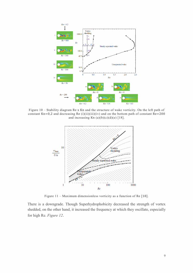
Figure 10 – Stability diagram Re x Kn and the structure of wake vorticity. On the left path of constant Kn=0,2 and decreasing Re (i)(ii)(iii)(iv) and on the bottom path of constant Re=200

and increasing Kn (a)(b)(c)(d)(e) [18].

Figure 11 – Maximum dimensionless vorticity as a function of Re [18].

There is a downgrade. Though Superhydrophobicity decreased the strength of vortex shedded, on the other hand, it increased the frequency at which they oscillate, especially for high Re. Figure 12.

9

Figure 12 – Normalized St* as a function of normalized Kn by its critical value for Re = 50 (square); 100 (diamond); 200(up triangle); 500(down triangle) and 800(star) [18].

Legendre explained perfectly the influence of slip length for a stationary cylinder, but for the case of elastic mounted cylinder VIM (Vortex-induced motions) credits for Daniello et. all. [19].

In their work [19], as expected from weaken of vortex shedding, the amplitude ratio (𝐴𝐴∗ = 𝐴𝐴𝑦𝑦/𝐷𝐷) , perpendicular to the flow, reduced up to 15% compared to a smooth cylinder. The greatest reduction was at the maximum oscillation, around reduced velocity of 𝑈𝑈∗ = 𝑈𝑈/𝑓𝑓𝑁𝑁𝐷𝐷 = 5,7. See Figure 13

Another fact, not intuitive at all, was the unaffected decay rate and, not so surprising, the same structural damping and frequency of induced oscillation. See Figure 14

Figure 13 - Reduced amplitudes over a rage of Re for Superhydrophobic cylinder (triangle -green) and smooth cylinder (square - red) [19].

10

Figure 14 - Decay test for superhydrophobic on the left (a) and smooth (b) [19].

Daniello et. all. also predict a problem that could not be analyzed for lacking the low end resolution in the study. Despite the delayed onset, the higher shedding frequency would reach the natural frequency of the cylinder earlier thus provoking onset of oscillation in lower Re.

Figure 15 - Frequency of vortex induced oscillations for superhydrophobic (triangle) and smooth (square) [19].

11

Figure 16 – Vortex shedding and lock-in presented by Daniello [19] for stationary no-slip (white square),stationary superhydrophobic (white triangle), oscillating no-slip (black square)

and oscillating superhydrophobic (gray triangle).

It is important to note that, as mentioned, the superhydrophobicity could delay both the onset of separation and the onset of vortex shedding, but they still occur in a higher frequency.

12

3. QUESTIONING THE LACK OF FLUID-SOLID FORCES

When we want to characterize the mechanical behavior of the flow, the first unknown variable kept in mind is the velocity vector field (𝐕𝐕), the most important property of the flow.

The velocity vector field is not an independent variable and straight relations with other properties of the fluid lie in its dependency, most of them thermodynamic properties.

Books like Frank M. White [20] document those thermodynamic properties as being pressure (p) , density (𝜌𝜌) and temperature (Θ) , but other secondary properties are extremely relevant, especially for computing frictional effects, such as the viscosity(𝜇𝜇) .

Other attribute, also documented, may induce disturbances in the velocity vector field causing influences on the behavior of the flow, but instead of being property of the fluid it belongs to the solid, the surface roughness.

Raising the question of the chapter’s title, no equation or condition was found to account for increases in adhesion forces, mainly attraction (normal to the surface), exerted in the fluid by the solid, except for the condition 𝐕𝐕 = 0 at the surface of the body independently of the material or the fluid viscosity.

Most of the conditions set for viscous fluid problems are no-slip condition everywhere in the surface regardless of the material of the body, i.e. the interaction forces. The chapter 1.3 showed that things could be a little bit different for some materials.

The closest we have done so far, was a special consideration for superhydrophobic materials expressed by (5). However, note that it does not provide any relation to its force components, only the velocity at the wall as if there is no influence on the fluid forces, i.e. the stickiness to the body. The identification of those forces of attraction (stickiness) by their effects on the dynamics of the flow is one of the goals of this project.

The investigation on lowering those forces, if present, is represented by the superhydrophobic experiment. Enough information was collected in chapter 2 pointing out the superhydrophobic property influence on the dynamics of the flow, such as delaying the onset (from leading edge) of vortex shedding and onset of separation and lowering vortex strength but in other hand increasing its frequency. This last consequence is of great importance since the author assumes that the main reason was the higher kinetic energy from less energy loss (slip length) corresponding also, in a counter way, to a lower adhesion forces (attraction of the water). Nevertheless, one experiment with superhydrophobic cylinder was conducted for this examination.

13

For the superhydrophilic investigation, no reference was found, but books and researches regularly quote about the influence of roughness to the fluid properties and the dynamics of the flow.

Taking Reynolds for example, Frank M .White’s book [20] cites that transition is highly dependent on surface roughness and increasing roughness causes earlier transition to a turbulent boundary layer.

Suitable for this work, the vortex shedding frequency expressed in terms of Strouhal, explained in chapter 5.1, is also dependent of cylinder roughness as cited in Anatol Roshko’s paper [21]. See Figure 17.

Figure 17 - Strouhal number as a function of Reynolds and surface characteristics [21].

All those previously described effects are correct and well presumed, but the reason does not seem to be the roughness itself. From the author’s point of view, one common shared misunderstanding about the roughness is that the nanoscopic or microscopic asperity of the surface causes an obstruction to the passage of the fluid element making the velocity near wall to be approximately zero.

However, from the author’s point of view, as explained in chapter 1.3 , the roughness could intensify, by increasing contact area between fluid and substrate, the hydrophobic or hydrophilic property, which in turn, diminishes or enhances the adhesion forces and that last consequence, is, from the author perspective, the main reasons behind all effects. Leading us to the Chapter 5.2 that describes the experiment and the method used to reach the hydrophilic property enabling the author to compare the results and later to conclude this work.

Not only enlightening the author’s comprehension, in chapter 4 the author will also predict benefits in hydrodynamics from handling them forces when applying hydrophobic and hydrophilic properties in specific regions of the solid body.

14

4. THE PROPOSITION EXPLAINED

Every other research so far, had led scientists to devote a great amount of effort at finding ways to increase the slip length so that we could reach, as seen in Figure 10, a high 𝐾𝐾𝑛𝑛 and consequently making the fluid behave like in potential theory.

However, as far as the author’s research could go, no material capable of producing the necessary slip-length was created. In addition, from the author’s perspective, it will not, except adding an external force and expending work.

Therefore, this project investigate two elastic mounted cylinders suffering from VIV, one for each property (superhydrophobic and superhydrophilic), and with enough data we will sustain the combine use of Superhydrophobicity and Superhydrophilicity to achieve a better condition in face of the problems or benefits arising from the flow.

For instance, one application would be in wing profiles like hydrofoil or fins and keels. According to the Daniel Bernoulli and the continuity equation, the water running over the top of the wing profile increases its velocity whereas in the bottom maintains the

stream velocity, this results in a pressure difference translated as the lift. Figure 18.

Figure 18 - Pressure-distribution on an airfoil section in viscous flow (dotted line) and inviscid (full line). [22].

Pressure is mainly caused by the collision of bodies, molecules or even vibrating atoms to an element of area. When water starts to flow over an area, the molecules become oriented, like electrons in a current, this reduces the collisions exerted in that area i.e. the pressure. Applying Superhydrophilicity to the bottom of the wing would create more frictional drag but at the same time, the pressure would increase, as the molecules would collide more. To compensate, introducing Superhydrophobicity over the top would reduce the frictional drag, thus increase the flow velocity and reduce the pressure. Therefore, the author predicts to get more efficiency from higher pressure gradient with approximately the same friction drag due to the equal gain and loss in this process.

15

Another application would interest the VIV (vortex-induced motion). The enhancement is more difficult to perceive and that is why the experiment in chapter 5.2 consists of such physics.

First, it is important to explain that the reasoning is not something new that no was has ever seen before. On the contrary, the author’s assumption explores the perception of a well-known scientist and a formula named after this prominent innovator, Osborne Reynolds (1842-1912). The formula is the following:

ℛ𝑒𝑒 =𝜌𝜌𝜌𝜌𝜌𝜌𝜇𝜇

(7)

In 1883 [23] Reynolds argued about the fact that no investigation or effort was done to trace the characteristics under the circumstances particular features of the fluid motion depended. Trying to find the reason and condition, which the resistance was sometimes proportional to square of velocity of moving bodies at high speed and as to velocity in capillary tubes at lower velocities, he started his work and proved the concept relation between inertia forces and viscous forces to fluid motion, which will sustain the present proposition.

Thus, in other words, the Reynold’s number is also the ratio between inertial forces and the viscous forces.

ℛ𝑒𝑒 =

𝐼𝐼𝐼𝐼𝐼𝐼𝐼𝐼𝐼𝐼𝐼𝐼𝐼𝐼𝐼𝐼 𝐹𝐹𝐹𝐹𝐼𝐼𝐹𝐹𝐼𝐼𝐹𝐹𝜌𝜌𝐼𝐼𝐹𝐹𝐹𝐹𝐹𝐹𝑢𝑢𝐹𝐹 𝐹𝐹𝐹𝐹𝐼𝐼𝐹𝐹𝐼𝐼𝐹𝐹

(8)

Resistance is proportional to square of the velocity when inertia forces are predominant at high ℛ𝑒𝑒 and to the velocity when viscous forces prevail, at low ℛ𝑒𝑒 . At different velocities with same geometry (geosims2) one can get either high resistance or low resistance, in other words, there is a transition.

If that is consent, maybe there is a situation where lowering the ℛ𝑒𝑒 number should produce less resistance, at the same stream velocity by just increasing the viscous contribution. That could be achievable by introducing a hydrophilic property at the surface of the body, the main topic of the proposition. With hydrophilic substrate, the viscosity of water in interfacial region could increase by a factor of 2 to 4 compared to bulk viscosity [24].

2 Term first suggested by Dr. E. V. Telfer

16

4.1. PHYSICS AND MATHEMATICS

A flat round object, like a disk, surrounded by water in a horizontal plane (neglect gravity), assuming that this horizontal plane is of infinite length and width, has a uniform pressure distribution along the surface 𝑃𝑃0.

Figure 19 – Representation of a disk immersed in water.

Now, if we were to make the water flow, we would note different results from increasing free stream velocity, e.g. the generation of vorticity. Those results are summarized in Figure 20 as a function of Reynold’s number.

Figure 20 - Regimes of fluid flows around a cylinder, modified image from [25].

The separation occurs because of the adverse pressure gradient inside the boundary layer. The point (A) where the velocity vector is perpendicular and the flow hits the

17

surface of the body, has velocity zero and highest pressure value (𝑃𝑃𝐴𝐴 > 𝑃𝑃0) as pressure increases proportionally to normal velocity component meaning more collisions. Points (B and D), where the velocity vector is tangent to the surface, reach the lowest pressure (𝑃𝑃𝐵𝐵,𝐷𝐷 < 𝑃𝑃0). Point (C) from inviscid theory should also reach the highest pressure. However, point (C) differs from point (A) where near stream velocity and the pressure gradient are both helping the fluid to get from (A) to (B) or (D).

On the way to point (C), the flow encounters an adverse pressure gradient and since part of the kinetic energy was lost due to shear effect, the flow separates. In addition, the near fluid is still passing around the body and pulls through viscous forces creating a strong and nonlinear interaction.

Figure 21 - Velocity profile near wall and separation sequence, modified image from [20].

18

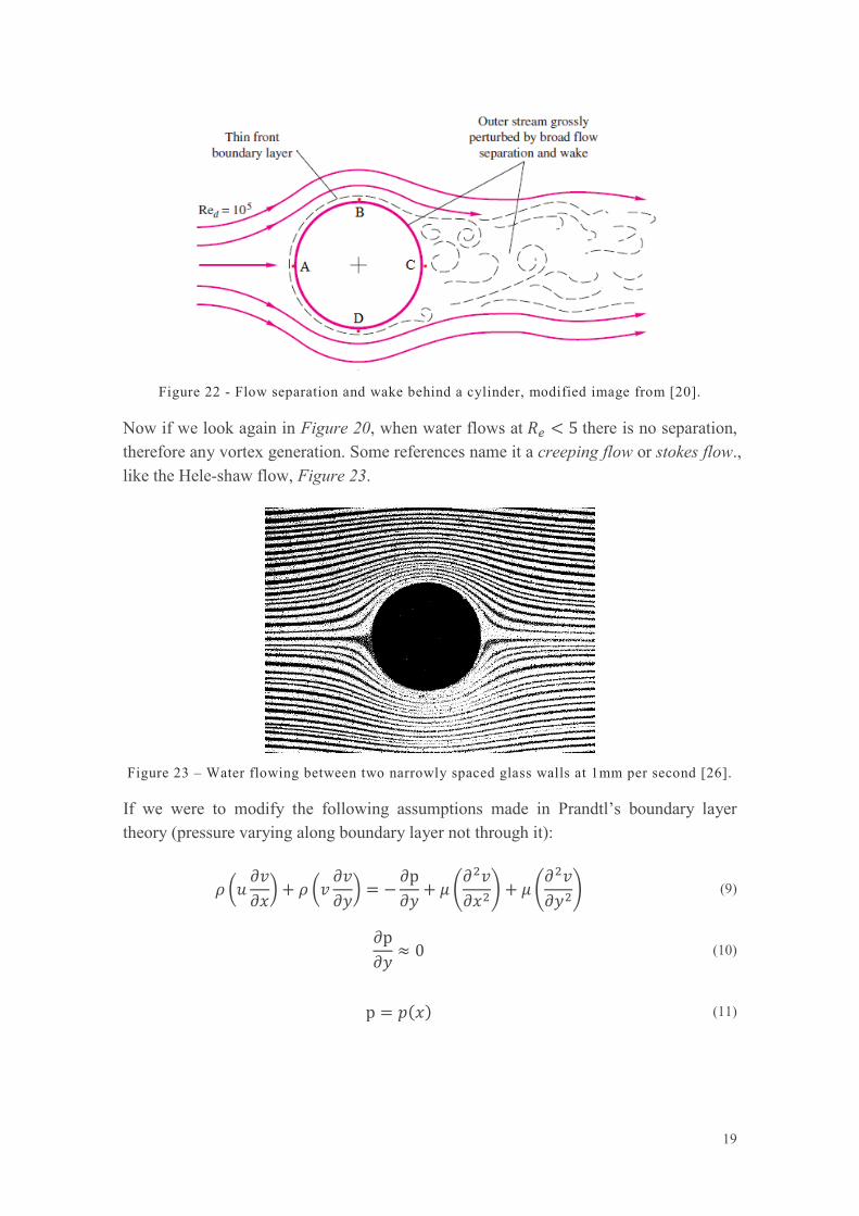
Figure 22 - Flow separation and wake behind a cylinder, modified image from [20].

Now if we look again in Figure 20, when water flows at 𝑅𝑅𝑒𝑒 < 5 there is no separation, therefore any vortex generation. Some references name it a creeping flow or stokes flow., like the Hele-shaw flow, Figure 23.

Figure 23 – Water flowing between two narrowly spaced glass walls at 1mm per second [26].

If we were to modify the following assumptions made in Prandtl’s boundary layer theory (pressure varying along boundary layer not through it):

𝜌𝜌 �𝑢𝑢

𝜕𝜕𝜕𝜕𝜕𝜕𝑑𝑑� + 𝜌𝜌 �𝜕𝜕

𝜕𝜕𝜕𝜕𝜕𝜕𝑦𝑦� = −

𝜕𝜕p𝜕𝜕𝑦𝑦

+ 𝜇𝜇 �𝜕𝜕2𝜕𝜕𝜕𝜕𝑑𝑑2

� + 𝜇𝜇 �𝜕𝜕2𝜕𝜕𝜕𝜕𝑦𝑦2

� (9)

𝜕𝜕p𝜕𝜕𝑦𝑦

≈ 0 (10)

p = 𝑝𝑝(𝑑𝑑) (11)

19

To another condition where only the inertia terms are neglected, meaning that both 𝑢𝑢 and 𝜕𝜕 velocity components are very small inside the boundary layer but their second order rate of change in respect of the two dimension are not.

∇𝐩𝐩 = µ∇2𝐕𝐕 (12)

𝜕𝜕p𝜕𝜕𝑦𝑦

≠ 0 (13)

Those equations mathematically stimulate the investigation, since there is a pressure gradient 𝑑𝑑𝑑𝑑

𝑑𝑑𝑦𝑦≠ 0 there is also forces acting, and since energy is always lost through

friction, the viscous forces, second term in (12), should suppress the adverse pressure along x-axis as in Hele-shaw flow.

Moreover, since viscous forces are proportional, in this work, to interaction forces between molecules and interface forces between solid and fluid, it is suggestive that hydrophobic and hydrophilic properties could in fact make a difference on the dynamics of the flow, not only for low 𝑅𝑅𝑒𝑒 but also for all cases. As expressed in navier-stokes equations (neglect gravity and local acceleration).

∇𝐩𝐩 = −𝜌𝜌(𝐕𝐕.∇)𝐕𝐕 + 𝜇𝜇∇2𝐕𝐕 (14)

∇𝐩𝐩 ∝ −(𝐼𝐼𝐼𝐼𝐼𝐼𝐼𝐼𝐼𝐼𝐼𝐼𝐼𝐼 𝑓𝑓𝐹𝐹𝐼𝐼𝐹𝐹𝐼𝐼𝐹𝐹) + (𝜕𝜕𝐼𝐼𝐹𝐹𝐹𝐹𝐹𝐹𝑢𝑢𝐹𝐹 𝑓𝑓𝐹𝐹𝐼𝐼𝐹𝐹𝐼𝐼𝐹𝐹) (15)

Therefore, this project studies the use of superhydrophilic properties in other to increase the stickiness of the fluid, maybe reducing vortex-shedding frequency along with increase of its strength, reducing the pressure drag, and finally achieving a better hydrodynamic efficiency. Just like in the wing profile method, balancing the loss of kinetic energy to frictional drag and strengthening of vortex from the Superhydrophilicity with the unstrengthening of vortex and decrease of frictional drag from Superhydrophobicity will create an even condition.

That goes against the common knowledge and sense, as if increasing the frictional resistance in a body would produce a better hydrodynamic efficiency.

Reynolds already glimpsed this fact when he heated water from five degrees (5º) to forty-five degrees (45º) and quoted:

“The more viscous a fluid is, the less prone is it to eddying or sinuous motion.” [23]

The exact manner of how water moves or behaves is too complicated and difficult to perceive and just presume, so to validate all propositions so far, this work makes use of a VIV experiment, described in chapter 5.1, using three cylinders with entirely different surfaces, which are smooth, superhydrophobic and superhydrophilic.

20

5. ABOUT THE EXPERIMENTS

5.1. VORTEX INDUCED VIBRATIONS

Vortex Induced Vibration (VIV) is a consequence from the pressure fluctuation and the

vortex shedding which excites the inelastic or elastic mounted body.

Jhon William Strut made the first public document regarding vibration effects in 1877,

at the time treated as third Baron Rayleigh. The Lord Rayleigh, explained one of the

main effects of vibration: The emission of sounds. Rayleigh [27] noted the irrevocable

correlation between vibration and sound emission and indicated the need of medium

(particles) for its propagation and an exciting force.

Subsequently in 1878 Vicence Strouhal made the first experimental study regarding

vortex induced vibrations. Strouhal [28] found out that a taut wire moving in air was

able to emit sounds (eolian tones) later he discovered that those sounds depended only

on the wire diameter and the airstream velocity. Strouhal also noted that the eolian tones

increased when on the natural frequency of the wire.

The mechanism created by Vicenc Strouhal consisted of a vertical apparatus ‘K’ made

of wood connected to two horizontal bars ‘A’ linked together by a taut wire ‘M’ and

fixed to a rotatory support ‘S’. Figure 24 shows the Strouhal’s device.

Figure 24 - Vicenc Strouhal mechanism sketch [28]

From his work, Strouhal introduced the strouhal number (St) which relates the

frequency of vortex shedding (𝑓𝑓𝑠𝑠) to the velocity of the flow over a stationary cylinder.

21

𝑆𝑆𝑡𝑡 =𝑓𝑓𝑠𝑠 × 𝐷𝐷𝑈𝑈

(16)

Subsequently Henri Claude Bénard, in 1908, correlated the work of Strouhal with two

nearly parallel rows of vortices behind the cylinder, later Theodore Von Kármán, in

1911, gave his theory of the vortex street, and so forth research on this subject

continued.

In recent years, VIV has been studied with more endeavors because of its engineering

application on offshore structures like risers, umbilicals and spar platforms as reported

by Fábio Moreira [29].

5.2. ONE DEGREE OF FREEDOM – VIV EXPERIMENT

For this experiment, the cylinder moves transversely to the flow only, . That one degree

of freedom restrain is just to simplify the data analysis by which the author uses to

evaluate and compare the phenomena in smooth (𝑆𝑆𝑆𝑆𝑂𝑂𝑂𝑂), superhydrophobic (𝑆𝑆𝐻𝐻𝑃𝑃𝐻𝐻𝑂𝑂)

and superhydrophilic (𝑆𝑆𝐻𝐻𝑃𝑃𝐻𝐻𝐼𝐼) surface cylinder, thereby showing the influence of such

property. The experiment representation is a mass-spring-damp system, Figure 25.

Figure 25 - Representation of the 1DOF experiment.

22

Figure 26 - Photo of the SHPHI cylinder prepared for test.

For the VIV study of an elastic mounted cylinder is very important to specify the mass ratio or relative density (𝑚𝑚∗), this non-dimensional number together with the damping ratio of the system (𝜁𝜁) is the main conductor of the type of the results that are to come. The peak amplitude depends principally on mass-damping, 𝜁𝜁 × 𝑚𝑚∗, whereas the regime of synchronization3, for a given mass-damping, depends primarily on mass ratio 𝑚𝑚∗ [30].

Figure 27 - Amplitude response A* versus normalized velocity U* for low mass ratio, 𝑚𝑚∗ = 10,1 in black squares and higher mass ratio in circles 𝑚𝑚∗ = 250 [29].

Feng (1968) experiments, in the air, had very large mass ratio (m∗~250), as for Khalak & Williamson (1999) low mass ratio (m∗ = 2,4 𝐼𝐼𝐼𝐼𝑑𝑑 10,3 𝐼𝐼𝐼𝐼𝑑𝑑 20,6), therefore even though the experiments were typically the same, the phenomena were proven distinct

3 Also known as “lock in”.

23

[31]. Note that, Figure 27 , Feng’s plot has two branches classified by initial branch and lower branch while Khalak & Williamson have three branches initial, upper and lower. Those branches occur in a condition called synchronization or “Lock in”. Initially in static position, when we increase the stream velocity 𝑈𝑈∗ the elastic mounted cylinder starts to suffer from monoscillating vortex shedding created with frequency 𝑓𝑓0, which values are just like of those in Strouhal experience for fixed cylinder. Note that, Figure

17, 𝑆𝑆𝑡𝑡 number is approximately 0,21 thus the expression 𝑈𝑈𝑓𝑓𝐷𝐷

nears 5.

If that shedding frequency 𝑓𝑓0 nears the natural frequency of the system, 𝑓𝑓𝑁𝑁 , both frequencies synchronize and the cylinder starts oscillating. Further increase in stream velocity U*, inside the range of synchronization, pulls the shedding frequency 𝑓𝑓0 away from the monoscillating value (St line). It means that, the cylinder then oscillates in a specific frequency 𝑓𝑓, in the synchronized range, and at the same time holds the vortex shedding frequency 𝑓𝑓0 . For high mass ratio, the oscillation frequency 𝑓𝑓 and the shedding frequency remain close to 𝑓𝑓𝑁𝑁 and thus the ratio 𝑓𝑓∗ = 𝑓𝑓/𝑓𝑓𝑁𝑁 remains close to unity, but for low 𝑚𝑚∗ values it could exceed the natural frequency by hundreds. Either way, the “lock-in” then brings high amplitudes with nearly constant frequency. Figure 28

Figure 28 - Frequency response for a range of mass ratios, m*, through the synchronization regime [30].

For means of comparison all cylinders, smooth, superhydrophobic and superhydrophilic have the same mass ratio.

The formula of the mass ratio is:

24

𝑚𝑚∗ =𝑚𝑚𝑡𝑡

𝜌𝜌ℎ𝜋𝜋 𝐷𝐷2

4

(17)

Where the total mass of the vibrating system “𝑚𝑚𝑡𝑡” is composed mass of the cylinder, coupler and the equivalent mass of the carbon fiber rod. The density of the tank water is “ρ” , the diameter of the cylinder is “D” and the height of the water line (still water) measured from the bottom of the tank “ℎ”.

The calculation is in Annex I and the result is:

𝑚𝑚∗ ≅ 2,33

The restauration of the system is also the same for each one of the cylinders. The equivalent elastic constant of the two springs used (one on each side) represent the (𝑘𝑘) restoring component in the equation of motion of the system.

Equation of motion:

(𝑚𝑚 + 𝑚𝑚𝑎𝑎)�̈�𝑑 + 𝐹𝐹�̇�𝑑 + 𝑘𝑘𝑑𝑑 = 𝐹𝐹(𝐼𝐼) (18)

Equivalent elastics constant:

𝑘𝑘 ≅ 50,4 𝑁𝑁/𝑚𝑚 (19)

From decay tests and by the use of (20), deduced from the equation of motion of a damped free vibrating system in an still fluid, we calculate the mentioned damping ratio of the system 𝜁𝜁 , the natural angular frequency of the structure 𝑤𝑤𝑛𝑛 and the natural frequency of the system in water 𝑓𝑓𝑛𝑛. The decay graphs are all in Annex II.

𝐼𝐼−𝜁𝜁𝑤𝑤𝑛𝑛𝑡𝑡 = 𝐼𝐼−𝐶𝐶0𝑡𝑡 (20)

𝜁𝜁𝑤𝑤𝑛𝑛 = 𝐶𝐶0 (21)

To solve (21) for 𝜁𝜁 we need the value of the natural angular frequency of the structure, 𝑤𝑤𝑛𝑛, for which we use the following equations.

𝑤𝑤𝑑𝑑 = �1 − 𝜁𝜁2𝑤𝑤𝑛𝑛 (22)

𝑤𝑤𝑑𝑑2 = (1 − 𝜁𝜁2)𝑤𝑤𝑛𝑛2 (23)

𝑤𝑤𝑑𝑑2 = 𝑤𝑤𝑛𝑛2 − 𝜁𝜁2𝑤𝑤𝑛𝑛2 (24)

𝑤𝑤𝑛𝑛2 = 𝑤𝑤𝑑𝑑2 + 𝐶𝐶02 (25)

The decay angular frequency, 𝑤𝑤𝑑𝑑, is obtainable from the data plot (amplitude x time) by measuring the period length of one cycle 𝑇𝑇𝑑𝑑.

25

𝑤𝑤𝑑𝑑 =

2𝜋𝜋𝑇𝑇𝑑𝑑

(26)

At last, solving from (25) we get:

𝑓𝑓𝑛𝑛 =

𝑤𝑤𝑛𝑛2𝜋𝜋

(27)

Another important non-dimensional number is the reduced velocity (𝑈𝑈∗ ) which is widely used in the graphs. It considers the stream velocity 𝑈𝑈, the natural frequency of the system in water 𝑓𝑓𝑛𝑛 and the diameter of the cylinder 𝐷𝐷, as expressed below.

𝑈𝑈∗ =

𝑈𝑈𝑓𝑓𝑛𝑛𝐷𝐷

(28)

Plotting the amplitude ratio, 𝐴𝐴∗, against the reduced velocity, 𝑈𝑈∗, leave us with graphs such as Figure 27. The formula of amplitude ratio is the following:

𝐴𝐴∗ =

𝑦𝑦𝐷𝐷

(29)

Where 𝑦𝑦 corresponds to the displacement of the cylinder and 𝐷𝐷 the diameter.

The last non-dimensional number left to explain, is the frequency ratio 𝑓𝑓∗ . The frequency ratio is composed of the frequency of oscillation 𝑓𝑓 and the natural frequency of the system in the water 𝑓𝑓𝑛𝑛. The graph composed of frequency ratio 𝑓𝑓∗ over a range of reduced velocity 𝑈𝑈∗ summarizes perfectly the “lock-in” region.

𝑓𝑓∗ =

𝑓𝑓𝑓𝑓𝑛𝑛

(30)

Now we have all graphic tools to analyze the flow around an elastic mounted cylinder.

26

5.3. THE LAB

Experiments were assembled and executed in LOC (Waves and Flow Lab) at Federal University of Rio de Janeiro. The lab is part of the program “Programa de Engenharia Naval e Oceânica da COPPE – UFRJ” [32]. The professor responsible for coordinating the lab is also the advisor of this project, Prof. Dr. Antônio Carlos Fernandes, whom the author is very grateful.

In October 17th (2012) Prof. Antonio Carlos Fernandes welcomed in LOC Nick Newman, his old friend, who advised him at M.I.T (Massachusetts Institute of Technology), shown in Figure 29.

Figure 29 - Prof. Newman and Prof. Fernandes on the right

The extensions of the LOC’s water tank are 0,8 𝑚𝑚 deep, 1,5 𝑚𝑚 wide and around 24,0 𝑚𝑚 length. The pumps connected to the tank provide a maximum velocity of 0,65𝑚𝑚/𝐹𝐹 for a water lever of 0,5 𝑚𝑚.

27

5.4. EXPERIMENTAL SET UP

Thanks to the help of Prof. Cyro Ketzer Saul we got the superhydrophobic cylinder. Prof. Cyro provided the superhydrophobic cylinder used in the experiments using the method studied by Ezequiel Burkarter [33].

Ezequiel used electrospray and aerospray to place layers of polytetrafluoroethylene (PFTE) over fluorine doped tin oxide (FTO) which produced contact angle of more than 150º. The SHPHO cylinder was created applying such layer at an aluminium tube of external diameter of ∅75 mm.

Most methods developed to create surfaces with superhydrophobic property are expensive and use extensive materials or chemical expertise and equipment. There have been efforts made to overcome this problem and this work would like to elucidate, for future research in the field, the method described by Nilsson et.al. [34] that definitely succeeded by using polytetrafluoroethylene (PTFE) and sandpaper.

TEFLON or polytetrafluoroethylene (PTFE) round tubes if sanded circumferentially4 (direction of the flow) with 240 grit would reveal superhydrophobicity property. The 240 sandpaper shows the highest advancing and receding5 contact angle Figure 30.

Figure 30 - Sandpaper used and the resulting surface roughness and resulting contact angles advancing and receding (wetting properties) [34].

The smooth cylinder (𝑆𝑆𝑆𝑆𝑂𝑂𝑂𝑂) was made with polyvinyl chloride (PVC) with a black paint cover to reduce errors caused by diffraction when acquiring data with the software Qualisys. The PVC cylinder has an external diameter of ∅75 mm.

The superhydrophilic cylinder (𝑆𝑆𝐻𝐻𝑃𝑃𝐻𝐻𝐼𝐼) was kind of a problem. An inquiry of papers on the area of material science was done to find an easy and cheap way to produce the superhydrophilic surface, but no such work was found. Therefore, another proposal was set to create the same behavior. Porously first aid tape with tiny threads was glued to present a superhydrophilic property from its rough material. The expectation behind the

4 Orientation of the nano ridges affects the separation point and vortex shedding frequency [39]. 5 In dynamics contact angles the drop presents one angle at the forward end and one at aft.

28

use of these adhesive is to enhance the adhesion of water at the cylinder’s surface by the absorption and adsorption of water by the cloth surface composed of microspores and microfilaments.

The elastic mounted cylinder 1DOF experiment was conducted by constraining the movement in the flow direction (‘x’ axis) and letting it oscillate perpendicular to the flow (‘y’ axis). One coupling makes the connection of the rod to the cylinder. Two identical linear springs were affixed to the coupling and to each side of the tank, adjusting the natural frequency to the velocity generated by the tank pumps.

The carbon fiber rod has a length of 3,145 𝑚𝑚 and weights 1,58 𝐾𝐾𝐾𝐾. The total length of the assembled system is 3,91 𝑚𝑚 and this value allows neglecting the rotation effect [29].

Figure 31 - First aid tape used to ennhance hyrophilic behavior.

Finally, to turn this conjecture into a real perceptible fact the next topic presents the results from the VIV experiment comprising all cylinders.

5.5. RESULTS

Free decay tests provided the correlation between the cylinders and their decay rate, damping frequency and natural frequency.

Decay test amplitudes were measured by the Qualisys and in a excel worksheet, a filter (macro) was created to plot only the peak amplitudes and then fitted an exponential

regression. See graphs in 9.2.

The damping frequency of each cylinder was:

𝑓𝑓𝑑𝑑(𝑆𝑆𝑆𝑆𝑂𝑂𝑂𝑂) ≅ 0,546 𝐻𝐻𝐻𝐻 (31) 𝑓𝑓𝑑𝑑(𝑆𝑆𝐻𝐻𝑃𝑃𝐻𝐻𝐼𝐼) ≅ 0,546 𝐻𝐻𝐻𝐻 (32)

𝑓𝑓𝑑𝑑(𝑆𝑆𝐻𝐻𝑃𝑃𝐻𝐻𝑂𝑂) ≅ 0,525 𝐻𝐻𝐻𝐻 (33)

We could assume that the damping frequency is the same as the natural frequency of the system (𝑓𝑓𝑑𝑑 ≈ 𝑓𝑓𝑛𝑛) because this assumption is valid for low values of damping ratio, but either way the calculation of those values were performed .

29

With the decay exponent provided by Microsoft Excel and (21) to (25) we find the natural frequency of each system in water and damping ratio:

Natural frequency:

𝑓𝑓𝑛𝑛(𝑆𝑆𝑆𝑆𝑂𝑂𝑂𝑂) ≅ 0,546 𝐻𝐻𝐻𝐻 (34)

𝑓𝑓𝑛𝑛(𝑆𝑆𝐻𝐻𝑃𝑃𝐻𝐻𝐼𝐼) ≅ 0,546 𝐻𝐻𝐻𝐻 (35)

𝑓𝑓𝑛𝑛(𝑆𝑆𝐻𝐻𝑃𝑃𝐻𝐻𝑂𝑂) ≅ 0,525 𝐻𝐻𝐻𝐻 (36)

The damping ratio:

𝜁𝜁(𝑆𝑆𝑆𝑆𝑂𝑂𝑂𝑂) ≅ 0,009 (37) 𝜁𝜁(𝑆𝑆𝐻𝐻𝑃𝑃𝐻𝐻𝐼𝐼) ≅ 0,024 (38) 𝜁𝜁(𝑆𝑆𝐻𝐻𝑃𝑃𝐻𝐻𝑂𝑂) ≅ 0,013 (39)

It is noticeable that the transformation of SMOO into SHPHI brings no change in the natural frequency of the system. However, we can state that the dumping ratio increased when applied the tape to enhance the hydrophilic property.

A small increase in SHPHO’s natural frequency and damping ratio is noticeable but as proven by Daniello [19] superhydrophobicity plays no influence on them, see Figure 14. Therefore, the difference is due to the material of its cylinder (aluminum) and the weight distribution inside it.

The amplitude of oscillation over diameter (𝐴𝐴∗ ) against normalized velocity (𝑈𝑈∗) showed astonishing changes.

The results differs from presented by Khalak & Williamson [30] but shows a similarity with B.Stappenbelt [35], Figure 32, and Pedro Vilas [36].

.

Figure 32 – Comparing A* versus U* data for SMOO, modified image from Stappenbelt [35].

30

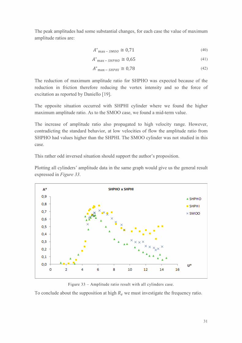
The peak amplitudes had some substantial changes, for each case the value of maximum amplitude ratios are:

𝐴𝐴∗max− 𝑆𝑆𝑆𝑆𝑆𝑆𝑆𝑆 ≅ 0,71 (40)

𝐴𝐴∗max− 𝑆𝑆𝑆𝑆𝑑𝑑𝑆𝑆𝑆𝑆 ≅ 0,65 (41) 𝐴𝐴∗max− 𝑆𝑆𝑆𝑆𝑑𝑑𝑆𝑆𝑆𝑆 ≅ 0,78 (42)

The reduction of maximum amplitude ratio for SHPHO was expected because of the reduction in friction therefore reducing the vortex intensity and so the force of excitation as reported by Daniello [19].

The opposite situation occurred with SHPHI cylinder where we found the higher maximum amplitude ratio. As to the SMOO case, we found a mid-term value.

The increase of amplitude ratio also propagated to high velocity range. However, contradicting the standard behavior, at low velocities of flow the amplitude ratio from SHPHO had values higher than the SHPHI. The SMOO cylinder was not studied in this case.

This rather odd inversed situation should support the author’s proposition.

Plotting all cylinders’ amplitude data in the same graph would give us the general result expressed in Figure 33.

Figure 33 – Amplitude ratio result with all cylinders case.

To conclude about the supposition at high 𝑅𝑅𝑒𝑒 we must investigate the frequency ratio.

31

The frequency ratio 𝑓𝑓∗ for high mass ratio 𝑚𝑚∗ should stay near unit. However, for low structural mass system in water, low mass ratio 𝑚𝑚∗, such as the present work, it diverges to other values as seen in Williamson & Govardan [31] 𝑓𝑓∗ = 1,4 , see Figure 34.

Figure 34 – Frequency ratio versus reduced velocity from Williamson & Govardan [31].

The frequency ratio in all cases had the same performance, a linear increase just after the synchronization of vortex frequency with natural frequency and with further increase in reduced velocity an approximately constant value.

If we compare the linear relation between the rate of change of frequency ratio in respect to the rate of change of reduced velocity or in other words the rate of change of vortex shedding frequency in respect to stream velocity, since natural frequency and diameter are constant, (43).

𝑑𝑑𝑓𝑓∗

𝑑𝑑𝑈𝑈∗ = 𝐷𝐷𝑑𝑑𝑓𝑓𝑑𝑑𝑈𝑈

(43)

We would notice for each case, see (44), (45), (46):

𝑑𝑑𝑓𝑓∗

𝑑𝑑𝑈𝑈∗ (𝑆𝑆𝑆𝑆𝑂𝑂𝑂𝑂) ≅ 0,072 (44)

𝑑𝑑𝑓𝑓∗

𝑑𝑑𝑈𝑈∗ (𝑆𝑆𝐻𝐻𝑃𝑃𝐻𝐻𝑂𝑂) ≅ 0,060 (45)

𝑑𝑑𝑓𝑓∗

𝑑𝑑𝑈𝑈∗ (𝑆𝑆𝐻𝐻𝑃𝑃𝐻𝐻𝐼𝐼) ≅ 0,096 (46)

The increase of the vortex shedding frequency was proportional to the increase of hydrophilic property. In the same procedure, if we compare the mean values in the range of practically constant frequency ratio, i.e. vortex shedding frequency, we will notice that:

32

𝑓𝑓∗���(𝑆𝑆𝑆𝑆𝑂𝑂𝑂𝑂) ≅ 1,384 (47) 𝑓𝑓∗���(𝑆𝑆𝐻𝐻𝑃𝑃𝐻𝐻𝑂𝑂) ≅ 1,240 (48) 𝑓𝑓∗���(𝑆𝑆𝐻𝐻𝑃𝑃𝐻𝐻𝐼𝐼) ≅ 1,343 (49)

As seen above, removing the odd result from SMOO case from the evaluation, there was an increase in the constant value of vortex shedding frequency from the SHPHO to SHPHI case.

Therefore, that result does not sustain the author’s supposition where the superhydrophilicity would hold back the capacity of vortex generation by increasing the viscous forces contribution from the strengthening of interaction forces between solid and fluid mainly adhesion forces.

Plotting all cylinders’ frequency data in the same graph would give us the general result expressed in Figure 35.

Figure 35 – Frequency ratio of all cases as function of reduced velocity.

33

6. CONCLUSION

At the end of this work, we gathered enough information firmly assuring that the forces at the interface between solid and fluid, exemplified by the material properties of superhydrophobicity and superhydrophilicity, could in fact change the dynamics of the flow, as seen in [15] [16] [17] [18] [19].

From the vortex induced vibrations experiments, in respect to the amplitude of oscillations, the results showed, except by the initial branch, a substantial reduction and enlargement of amplitude related to diminished and enhanced adhesion forces by the use of superhydrophobic and superhydrophilic cylinder respectively.

As to vortex shedding frequency, the results proved that the superhydrophobic property, just after the synchronization with the natural frequency, reduced the rate of change of vortex shedding frequency in respect with the stream velocity and the mean value in the constant frequency range. Whereas the superhydrophilic property was precisely the opposite, corresponding to an increase in rate and in the mean value on the constant frequency range.

Therefore, it is fair to conclude that, for the author’s supposition of superhydrophilicity reducing the vortex generation by increasing the viscous forces contribution from the strengthening of interaction forces (attraction) between solid and fluid would not, for high 𝑅𝑅𝑒𝑒, reduce the pressure drag and achieve a better efficiency.

However, the flow regime, at most condition generated by the tank, was already in turbulence transition and the porous cloth tape, which provided the superhydrophilic property, was entirely covering the cylinder, not just its rear. In addition, the porous cloth tape absorbed the water mimicking the superhydrophilicity not truly setting it from adsorption.

Notwithstanding, an overwhelming (“mind-boggling”) result occurred in the lower end of the experiments where the superhydrophobic cylinder had a higher amplitude ratio in comparison with the superhydrophilic (𝐴𝐴∗ ≅ 0).

To finish the author leave the question of controlling the use of those properties, for instance just in the cylinder’s rear, and the influence on the vortex shedding generation in lower 𝑅𝑅𝑒𝑒 to future students and researches.

34

7. REFERENCES

[1] B. Arkles, "Hydrophobicity, Hydrophilicity and Silanes," [Online]. Available: http://www.gelest.com. [Accessed October 2014].

[2] M. F. A. Rahman, "URRG - Underwater Robotics Reaserch Group," [Online]. Available: http://urrg.eng.usm.my/. [Accessed 10 2014].

[3] Y. Yuan and T. R. Lee, "Contact Angle and Wetting Properties," Springer Series in Surface Sciences, p. 33, 2013.

[4] SITA Process Solutions 2013, "SITA Process Solutions," SITA Messtechnik GmbH, 2013. [Online]. Available: http://surface-tension.sita-process.com/overview/. [Accessed 2014].

[5] K. László, Physical Chemistry of Surfaces, Budapest, 2014.

[6] "Wikipedia," Wikimedia Foundation, Inc., [Online]. Available: http://en.wikipedia.org/wiki/Contact_angle.

[7] T. Young, "An Essay on the Cohesion of Fluids," London, 1805.

[8] W. Barthlott and C. Neinhuis, "Purity of sacred lotus, or escape from contamination in biological surfaces," Planta - An International Journal of Plant Biology, no. 202, pp. 1-8, 1997.

[9] P. Roach, N. J. Shirtcliffe and M. I. Newton, "Progress in Superhydrophobic Surface Development," Soft Matter, 30 October 2007.

[10] D. C. Tretheway and C. D. Meinhart, "Apparent Fluid Slip at Hydrophobic Microchannel Walls," Physics of Fluids, vol. 14, March 2002.

[11] S. Lyu, D. C. Nguyen, D. Kim, W. Hwang and B. Yonn, "Experimental Drag Reduction Study of Super-hydrophobic Surface with Dual-scale Structures," Applied Surface Science, pp. 206-2011, 16 September 2013.

[12] C. Cottin-Bizonne, J. L. Barrat, L. Bocquet and É. Charlaix, "Low-friction Flows of Liquid at Nanopatterned Interfaces," Nature Materials, vol. 2, pp. 237-240, April 2003.

[13] J. Ou, B. Perot and J. P. Rothstein, "Laminar drag reduction in microchannels using ultrahydrophobic surfaces," Physics of Fluids, 09 November 2004.

[14] C. Ybert, C. Barentin, C. Cottin-Bizonne, P. Joseph and L. Bocquet, "Achieving Large Slip with Superhydrophobic Surfaces: Scaling Laws for Generic Geometries," Physics of Fluids, vol. 19, 03 December 2007.

[15] A. K. Balasubramanian, A. C. Miller and O. K. Rediniotis, "Microstructured Hydrophobic Skin for Hydrodynamic Drag Reduction," AIAA Journal, pp. 411-414, February 2004.

[16] C. Henoch, T. N. Krupenkin, P. Kolodner, J. A. Taylor, M. S. Hodes, A. M. Lyons, C. Peguero and K. Breuer, "Turbulent Drag Reduction Using Superhydrophobic Surfaces," AIAA, June 2006.

[17] K. Moaven, M. Rad and M. Taeibi-Rahni, "Experimental Investigation of Viscous Drag Reduction

35

of Superhydrophobic Nano-coating in Laminar and Turbulent Flows," Experimental Thermal and Fluid Science, pp. 239-243, 12 2013 August.

[18] D. Legendre, E. Lauga and J. Magnaudet, "Influence of Slip on the Dynamics of Two-Dimensional Wakes," Journal of Fluid Mechanics, vol. 63, pp. 437-477, 25 March 2009.

[19] R. Daniello, P. Muralidhar, N. Carron, M. Greene and J. P. Rothstein, "Influence of Slip on Vortex-induced Motion of a Superhydrophobic Cylinder," Journal of Fluids and Structures, pp. 358-368, 13 August 2013.

[20] F. M. White, Fluid Mechanics, 7 ed., New York: Inc. McGraw-Hill Companies, 2008.

[21] A. Roshko, "On the Development of Turbulent Wakes from Vortex Streets," California, 1954.

[22] E. L. Houghton and P. W. Carpenter, Aerodynamics for Engineering Students, Oxford: Butterworth Heinemann, 2003.

[23] O. Reynolds, "An Experiental Investigation of the Circumstances Which Determine Whether the Motion of Water Shall be Direct or Sinuouos, and the Law of Resistance in Parallel Channels," Philosophical Transactions of the Royal Society, 1883.

[24] C. Sendner, D. Horinek, L. Bocquet and R. R. Netz, "Interfacial Water at Hydrophobic and Hydrophilic Surfaces: Slip, Viscosity and Diffusion," Langmuir, pp. 10768-10781, 10 July 2009.

[25] P. A. Techet, "MIT OpenCourseWare," 28 November 2001. [Online]. Available: http://ocw.mit.edu/courses/mechanical-engineering/2-22-design-principles-for-ocean-vehicles-13-42-spring-2005/index.htm. [Accessed January 2015].

[26] M. V. Dike, An Album of Fluid Motion, Stanford: The Parabolic Press, 1982.

[27] B. R. M. F. John William Strutt, The Theory of Sound, vol. I, Cambridge, London: Macmillan and Co., 1877, p. 326.

[28] D. V. Strouhal, "Über Eine Besondere Art der Tonerregung," Würzburg, 1878.

[29] F. M. Coelho, "Porosidade Dirigida no Controle de Vibrações Induzidas por Vórtice em Aplicações com Um e Dois Graus de Liberdade," p. 121, Julho 2010.

[30] A. Khalak and C. H. K. Williamson, "Motions, Forces and Mode Transitions in Vortex-Induced Vibrations at Low Mass-Damping," Journal of Fluids and Structures, pp. 813-851, 9 July 1999.

[31] C. H. Williamson and R. Govardhan, "Vortex-Induced Vibration," Annual Review of Fluid Mechanic, pp. 413-455, 2004.

[32] A. C. Fernandes, "LOC - Laboratório de Ondas e Correntes," [Online]. Available: http://www.oceanica.ufrj.br/loc/. [Accessed October 2014].

[33] E. Burkarter, “Desenvolvimento de Superfícies Superhidrofóbicas de Politetrafluoretileno,” Curitiba, 2010.

[34] M. A. Nilsson, R. J. Daniello and J. Rothstein, "A Novel and Inexpensive Techinique for Creating Superhydrophobic Surfaces Using Teflon and Sandpaper," Journals of Physics D: Applied Physics , 12 January 2010.

36

[35] B. Stappenbelt, F. Lalji and G. Tan, "Low Mass Ratio Vortex-Induced Motion," in 16th Australasian Fluid Mechanics Conference, Gold Coast, 2007.

[36] P. V. Boas, "Projeto de Graduação".

[37] P. Muralidhar, N. Ferrer, R. J. Daniello and J. P. Rothstein, "Influence of Slip on the Flow Past Superhydrophobic Circular Cylinders," Journal of Fluid Mechanics, pp. 459-476, 10 Agust 2011.

37

8. ANNEX I

For the total mass of the vibrating system (𝑚𝑚𝑡𝑡) one consideration has to be made. Since the system is composed of a cylinder connected to a rod, which oscillates in a pendulum motion, it is convenient to proper account for the distributed mass of the rod (𝑚𝑚𝑟𝑟𝑟𝑟𝑑𝑑 ). The rod, then, becomes as a concentrated point mass pendulum with an equivalent masse (𝑚𝑚𝑒𝑒).

For that, the new equivalent system must have the same mass moment of inertia as

the previous model (Ι𝑒𝑒𝑒𝑒 = Ι𝑠𝑠𝑦𝑦𝑠𝑠𝑡𝑡𝑒𝑒𝑠𝑠).

The moment of inertia of a uniform thin rod with mass (𝑚𝑚) and length (ℓ) about an axis on its end comes from the sum of the contribution of each point mass (Ι𝑝𝑝𝑟𝑟𝑝𝑝𝑛𝑛𝑡𝑡 𝑠𝑠𝑎𝑎𝑠𝑠𝑠𝑠) moment of inertia.

Ι𝑝𝑝𝑟𝑟𝑝𝑝𝑛𝑛𝑡𝑡 𝑠𝑠𝑎𝑎𝑠𝑠𝑠𝑠 = 𝑚𝑚 × 𝐼𝐼2 (50)

Ι = �𝑑𝑑Ι = �𝐼𝐼2 × 𝑑𝑑𝑚𝑚 (51)

The linear mass distribution (𝜆𝜆) is constant and equal to (𝑠𝑠ℓ

). Leaving (51) as follow:

38

𝑑𝑑𝑚𝑚 = 𝜆𝜆 𝑑𝑑𝐼𝐼 (52)

Ι𝑟𝑟𝑟𝑟𝑑𝑑 = �𝐼𝐼2 ×

𝑚𝑚𝑟𝑟𝑟𝑟𝑑𝑑

ℓ𝑑𝑑𝐼𝐼

ℓ

0

(53)

Solving the integral:

Ι𝑟𝑟𝑟𝑟𝑑𝑑 =𝑚𝑚𝑟𝑟𝑟𝑟𝑑𝑑 × ℓ2

3

(54)

For the equivalent system:

Ι𝑒𝑒𝑒𝑒 = 𝑚𝑚𝑒𝑒𝑒𝑒 × 𝐼𝐼2 (55)

Ι𝑒𝑒𝑒𝑒 = 𝑚𝑚𝑒𝑒𝑒𝑒 × (ℓ +ℎ2

)2 (56)

Finally, for Ι𝑒𝑒𝑒𝑒 = Ι𝑟𝑟𝑟𝑟𝑑𝑑, combining (54) and (56):

𝑚𝑚𝑒𝑒𝑒𝑒 × (ℓ +

ℎ2

)2 =𝑚𝑚𝑟𝑟𝑟𝑟𝑑𝑑 × ℓ2

3 (57)

ℓ = Length of the fiber rod, which is equal to ℓ = 3,145 𝑚𝑚

𝑚𝑚𝑟𝑟𝑟𝑟𝑑𝑑 = Mass of the fiber rod, which is equal to 𝑚𝑚𝑟𝑟𝑟𝑟𝑑𝑑 = 1,580 𝐾𝐾𝐾𝐾

ℎ = Height of the water line (still water) measured from the bottom of the tank, which is equal to ℎ = 0,50 𝑚𝑚.

𝑚𝑚𝑒𝑒𝑒𝑒 ≅

1,580 × 3,1452

3 × �3,145 + 0,502 �

2 (58)

𝑚𝑚𝑒𝑒𝑒𝑒 ≅ 0,452 𝐾𝐾𝐾𝐾 (59)

The total structural mass of the system (𝑚𝑚𝑡𝑡) is then equal to:

𝑚𝑚𝑡𝑡 = 𝑚𝑚𝑒𝑒𝑒𝑒 + 𝑚𝑚𝑐𝑐𝑟𝑟 + 𝑚𝑚𝑐𝑐𝑦𝑦 (60)

Where values are:

𝑚𝑚𝑐𝑐𝑟𝑟 = Mass of the coupler and springs, which is equal to 𝑚𝑚𝑐𝑐𝑟𝑟 = 1160 𝐾𝐾

𝑚𝑚𝑐𝑐𝑦𝑦 = Mass of the cylinder, which is equal to 𝑚𝑚𝑐𝑐𝑦𝑦 = 3540 𝐾𝐾

39

𝑚𝑚𝑡𝑡 ≅ 0,452 + 1,160 + 3,540 (61)

𝑚𝑚𝑡𝑡 ≅ 5,152 𝐾𝐾𝐾𝐾 (62)

Hence, the mass ratio (𝑚𝑚∗) expressed by (17) is equal to:

𝑚𝑚∗ =

5,152

1000 × 0,5 × 𝜋𝜋 × 0,07524

(63)

𝑚𝑚∗ ≅ 2,33 (64)

40

9. ANNEX II

In this annex, we provide visual information from the response graph of all decay experiments and the graphs of the peak amplitude (after macro filtering) with an exponential approximation line and equation.

9.1. DECAY GRAPHS

Two tests were conducted for each cylinder:

Smooth Cylinder

Figure 36 - First decay test for SMOO cylinder.

Figure 37 – Second decay test for SMOO cylinder

41

Superhydrophobic Cylinder

Figure 38 - First decay test for SHPHO cylinder.

Figure 39 – Second decay test for SHPHO cylinder

42

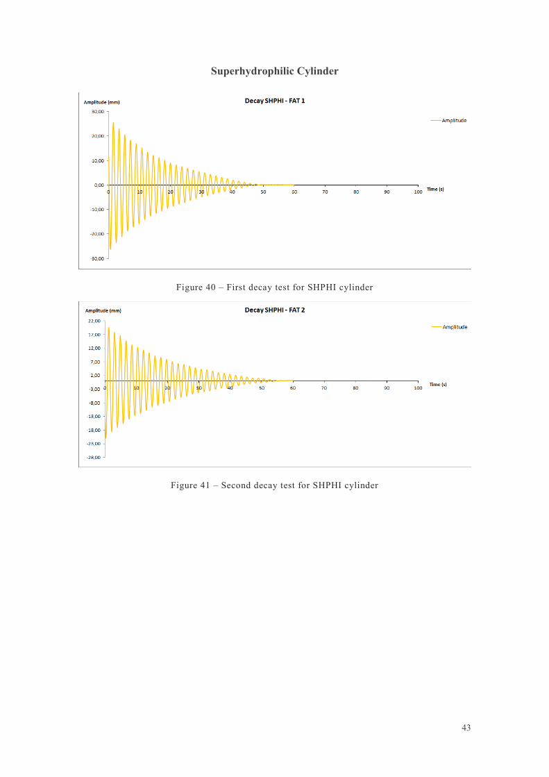
Superhydrophilic Cylinder

Figure 40 – First decay test for SHPHI cylinder

Figure 41 – Second decay test for SHPHI cylinder

43

9.2. PEAK GRAPHS AND EXPONENTIAL APPROXIMATION

Each amplitude decay test had a filter treatment to show only the positive peak amplitude and afterwards an exponential regression adjustment.

Smooth Cylinder

Figure 42 – Peak of amplitude in the first decay test for SMOO cylinder.

Figure 43 – Peak of amplitude in the second decay test for SMOO cylinder

44

Superhydrophobic Cylinder

Figure 44 - – Peak of amplitude in the first decay test for SHPHO cylinder

Figure 45 – Peak of amplitude in the second decay test for SHPHO cylinder

45

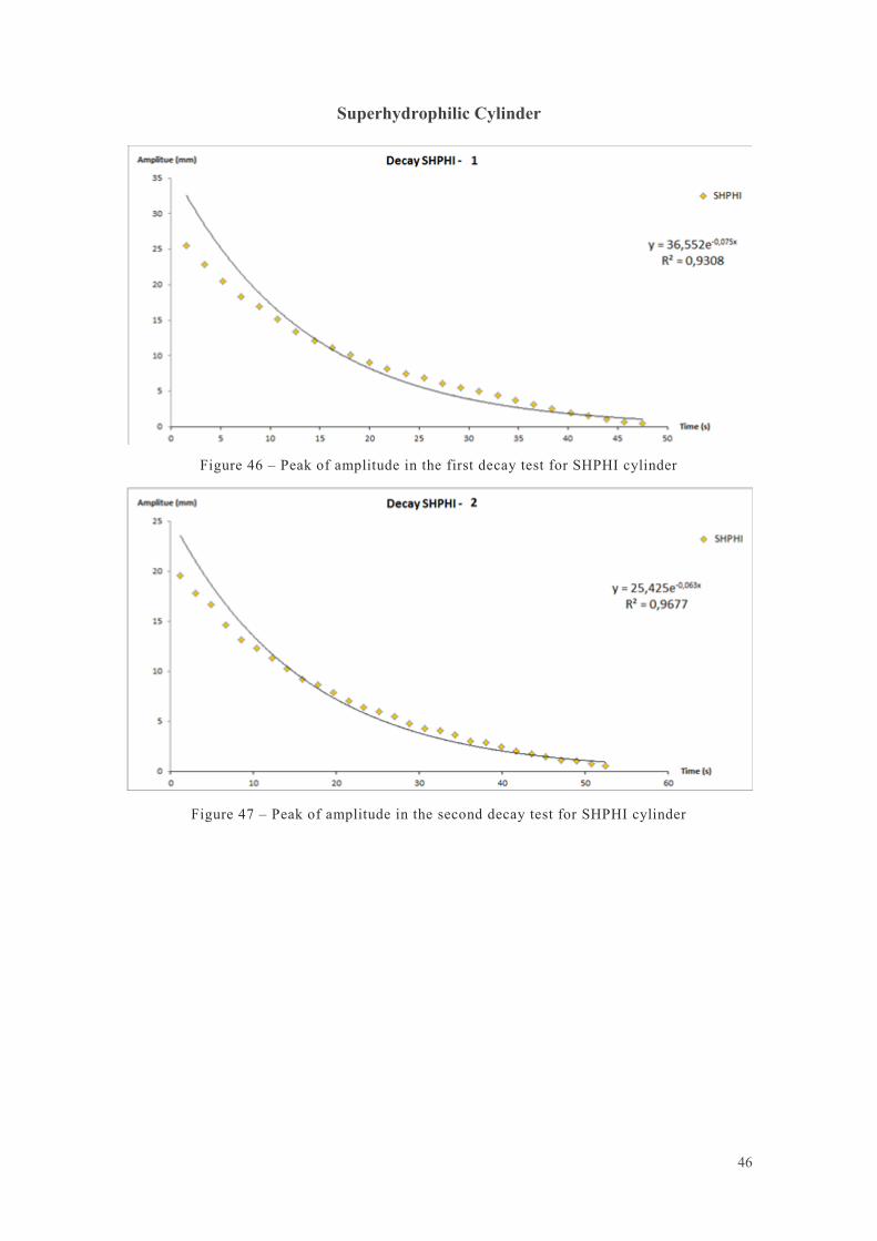
Superhydrophilic Cylinder

Figure 46 – Peak of amplitude in the first decay test for SHPHI cylinder

Figure 47 – Peak of amplitude in the second decay test for SHPHI cylinder

46

9.3. AMPLITUDE RATIO GRAPHS

The amplitude ratio against normalized velocity results from SMOO, SHPHI and SHPHO cylinder are:

Figure 48 – Amplitude ratio versus reduced velocity for SMOO cylinder

Figure 49 – Amplitude ratio versus reduced velocity for SHPHI cylinder

Figure 50 – Amplitude ratio versus reduced velocity for SHPHO cylinder

47

9.4. FREQUENCY RATIO GRAPHS

The frequency ratio against normalized velocity results from SMOO, SHPHI and SHPHO cylinder are:

Figure 51 – Frequency ratio versus reduced velocity SMOO case

Figure 52 – Frequency ratio versus reduced velocity SHPHI case

Figure 53 – Frequency ratio versus reduced velocity SHPHO case

48

9.5. VELOCITY TABLE

We provide, for future work, a table in excel worksheet with the velocity data over a range of rpm of each pump available in LOC’s water tank.

To achieve lower velocities it was necessary to turn off some of the pumps but in the condition of all pumps turned on, the present work increased by 100 rpm each pump producing an increased velocity corresponding to the picture of the table that follows.

49

50