Investigation of the Addition of Basalt Fibres into Cement

Western Kentucky UniversityTopSCHOLAR®

Masters Theses & Specialist Projects Graduate School

5-2014

Investigation of the Addition of Basalt Fibres intoCementJahi PalmeWestern Kentucky University, [email protected]

Follow this and additional works at: http://digitalcommons.wku.edu/theses

Part of the Engineering Physics Commons, and the Materials Chemistry Commons

This Thesis is brought to you for free and open access by TopSCHOLAR®. It has been accepted for inclusion in Masters Theses & Specialist Projects byan authorized administrator of TopSCHOLAR®. For more information, please contact [email protected].

Recommended CitationPalme, Jahi, "Investigation of the Addition of Basalt Fibres into Cement" (2014). Masters Theses & Specialist Projects. Paper 1361.http://digitalcommons.wku.edu/theses/1361

http://digitalcommons.wku.edu?utm_source=digitalcommons.wku.edu%2Ftheses%2F1361&utm_medium=PDF&utm_campaign=PDFCoverPages

http://digitalcommons.wku.edu/theses?utm_source=digitalcommons.wku.edu%2Ftheses%2F1361&utm_medium=PDF&utm_campaign=PDFCoverPages

http://digitalcommons.wku.edu/Graduate?utm_source=digitalcommons.wku.edu%2Ftheses%2F1361&utm_medium=PDF&utm_campaign=PDFCoverPages

http://digitalcommons.wku.edu/theses?utm_source=digitalcommons.wku.edu%2Ftheses%2F1361&utm_medium=PDF&utm_campaign=PDFCoverPages

http://network.bepress.com/hgg/discipline/200?utm_source=digitalcommons.wku.edu%2Ftheses%2F1361&utm_medium=PDF&utm_campaign=PDFCoverPages

http://network.bepress.com/hgg/discipline/135?utm_source=digitalcommons.wku.edu%2Ftheses%2F1361&utm_medium=PDF&utm_campaign=PDFCoverPages

INVESTIGATION OF THE ADDITION OF BASALT FIBRES INTO CEMENT

A Thesis

Presented to

The Faculty of the Department of Physics and Astronomy

Western Kentucky University

Bowling Green, Kentucky

In Partial Fulfillment

Of the Requirements for the Degree

Master of Science

By

Jahi Palmer

May 2014

I dedicate this thesis to my momma, Sabrina Palmer, for being awesome. To Crystal

Womack for being a friend for the seventeen years it took me to get to this point in my

life. To Kyle Gardner for being mine… I guess love is weird. Hmmm, I guess to

Brandon Jones since he’s my brother in ways that defy words. I am also dedicating this

to myself for doing the work that was required to make it happen.

iv

ACKNOWLEDGMENTS

It is tough to know who exactly to acknowledge when it comes to something that

requires this much work, but I will attempt to say something: I acknowledge Western

Kentucky University. I acknowledge the NOVA Center at WKU. This is where I did my

research. I also would like to acknowledge the Ghost Cat drawing. Whenever there was

a test with an answer that I couldn’t figure out, I would draw a ghost cat. If it hadn’t been

for that drawing, I never would have worked to find the answers. Lastly, there is an

entire list of friends to acknowledge, so I won’t even try to list them.

v

CONTENTS

Chapter 1 Introduction……………………………………………………………………1

1.1 History of Cement…………………………………………………………….1

1.2 Movitvation…………………………………………………………………...2

Chapter 2 Materials and Methods………………………………………………………...5

2.1 Materials………………………………………………………………………5

2.2 Proceedure…………………………………………………………………….5

2.2.1 Preparations………………................................................................6

2.3 Tools…………………………………………………………………………..7

2.3.1 Load Frame………………………………………………………….7

2.3.2 Load Cell…………………………………………………………….9

2.3.3 Lab View…………………………………………………………...11

2.3.4 Scanning Electron Microscope…………………………………….12

2.4 Basalt and Basalt Fibres……………………………………………………...15

Chapter 3 Results………………………………………………………………………...18

3.1 Tests at 53.7 m/min………………………………………………………...18

3.2 Tests at 67.2m/min………………………………………………………...22

3.3 Tests at 87.3 m/min………………………………………………………...26

3.4 Tests at 107.4 m/min……………………………………………………….30

3.5 Tests at 117.5 m/min……………………………………………………….34

Chapter 4 Conclusion……………………………………………………………………39

References……………………………………………………………………………….41

vi

LIST OF GRAPHS

Graph 3.1 53.7 micrometer/min deformation rate no fibres…………………………......19

Graph 3.2 53.7 micrometer/min deformation rate .06%...................................………….19

Graph 3.3 53.7 micrometer/min deformation rate .2%.........................................……….20

Graph 3.4 57.3 micrometer/min deformation rate .8%.....................................………….20

Graph 3.5 67.2 micrometer/min deformation rate no fibres……………………………..23

Graph 3.6 67.2 micrometer/min deformation rate .06%....................................................23

Graph 3.7 67.2 micrometer/min deformation rate .2%......................................................24

Graph 3.8 67.2 micrometer/min deformation rate .8%......................................................24

Graph 3.9 87.3 micrometer/min deformation rate no fibres……………………………..27

Graph 3.10 83.7 micrometer/min deformation rate .06%..................................................27



Graph 3.13 107.4 micrometer/min deformation rate no fibres…………………………..31

Graph 3.14 107.4 micrometer/min deformation rate .06%................................................31



Graph 3.17 117.5 micrometer/min deformation rate no fibres…………………………..35

Graph 3.18 117.5 micrometer/min deformation rate .06%................................................36



Graph 4.1 53.7 micrometer/min deformation rate stress and strain vs concentration…...34


vii


Graph 4.4 107.4 micrometer/min deformation rate stress and strain vs concentration.....37

Graph 4.5 117.5 micrometer/min deformation rate stress and strain vs concentration.....38

Graph 4.6 Comparison Graph…………………………………………………………....39

viii

LIST OF FIGURES

Figure 1.1 Concrete Sidewalk……………………………………………………………..3

Figure 2.1 Concrete Sample……………………………………………………………….6

Figure 2.2 Load Frame…………………………………………………………………….8

Figure 2.3a Steel Grip……………………………………………………………………10

Figure 2.3b Load Cell……………………………………………………………………10

Figure 2.4 LabVIEW…………………………………………………………………….11

Figure 2.5 Large Chamber Scanning Electron Microscope……………………………...13

Figure 2.6 Basalt Fibres at 349x Magnification………………………………………….14

Figure 2.7 Optical Microscope Image…………………………………………………...15

Figure 2.8 Basalt Rock…………………………………………………………………...16

ix

LIST OF TABLES

Table 1 Resulting RPMs…….…………………………………………………………….9

Table 2 Properties of Basalt Fibres…….………………………………………………...17

Table 3 Pertinent Information for Tests at Deformation Rate of 53.7 m/min…......…...21

Table 4 Pertinent Information for Tests at Deformation Rate of 67.2 m/min..………...25

Table 5 Pertinent Information for Tests at Deformation Rate of 87.3 m/min…..……...29

Table 6 Pertinent Information for Tests at Deformation Rate of 107.4 m/min………...33

Table 7 Information for Tests at Deformation Rate of 117.5 m/min…………...……...37

x

INVESTIGATION OF THE ADDITION OF BASALT FIBRES INTO CONCRETE

Jahi Palmer May 2014 42 Pages

Directed by: Edward Kintzel, Shane M. Palmquist, Keith Andrew

Department of Physics and Astronomy Western Kentucky University

Mechanical properties of concrete are most commonly determined using

destructive tests including: compression, flexure, and fracture notch specimen tests.

However, nondestructive tests exist for evaluating the properties of concrete such as

ultrasonic pulse velocity and impact echo tests. One of major issues with concrete

(which has cement as its prime ingredient) is that unlike steel it is quasi-brittle material.

It tends to want to crack when tensile stresses develop. Fibres have been added to

concrete for many years to reduce the amount of and size of cracks cause by temperature

changes or shrinkage. In more recent years, significant research has been carried out into

the effect of the addition of basalt fibres to cement has on its mechanical strength. As

well, developing concrete that is more durable, flexible, stronger, and less permeable than

traditional concrete has been explored. It has become important to test and verify

improvements that are made to the cement by basalt fibres as well as testing the general

strength of concrete to stand up to constant pressure at varied strengths.

1

CHAPTER 1 INTRODUCTION

Section 1.1 History of Cement

Merriam-Webster defines cement as a binding element or agency: as

a substance to make objects adhere to each other. Substances that meet this qualification

existed on earth naturally twelve million years ago. (University of Illinois.) As a building

material, concrete formed of mud and straw was used to bind dried bricks in order to

create the blocks of the pyramids of Egypt. During the same era of 3000 B.C. in China

and the Asias cementitious materials were being used to hold together bamboo for boats

as well as to create cricks for the Great Wall.

The Pantheon, created originally in ancient Rome and later rebuilt in 126 AD, is

still the world’s largest, unreinforced concrete dome at a diameter of 43.3 meters

(Claridge 1998.) Though tests have not been performed on the concrete that makes up

the Pantheon, tests from ancient Roman ruins show a compressive strength of 20 MPa

(Cowan 1977.) Compressive strength is defined as the capacity of a material or structure

to withstand loads tending to reduce size (National Institute of Standards and

Technology, NIST.) Standard modern concrete has a compressive strength ranging from

17 MPa to a possible 138 MPa (Portland Cement.)

After the fall of Rome, the usage and creation of cement and therefore concrete

was temporarily lost until the early 15th century when a more modern method of

producing hydraulic cement was developed by John Smeaton (Rosen 2012.) Smeaton

also identified the appropriate composition of lime to achieve a cement that would

eventually lead to the creation of Portland Cement by cement manufacturer Joseph

Aspdin in 1824.

2

The cement was named “Portland Cement” because Aspdin said that it resembled

Portland stone which was found locally and was used in most buildings throughout

England.

Section 1.2 Motivation

Since Industrial Revolustion starting in about 1760 many different types of

cement were used to create concrete until in 1900 testing of concrete was standardized

allowing for the strengths of different concretes (and the cements that bind them) to be

compared.

Concrete is the world’s most used building material. In 1960 synthetic fibres such

as polypropylene were added to concrete as a way to possibly increase its strength. It has

been shown (Metaxa, et al. 2010) that adding nanoscale fibres, specifically carbon

nanofibres, increases the compressive strength of concrete. However, nanoscale fibres

are difficult and expensive to create. The addition of an easier to produce, cheaper to

produce fibre to the cement would be a great benefit to builders of concrete structures.

A sidewalk is a commonly seen concrete structure. After years of usage the

structure begins to crack from either settling or from wear and tear. If the cement that

will ultimately create the concrete that makes the sidewalk has higher mechanical

strength, it may be possible to avoid cracking for a longer period of time. (Figure 1.1 is

an image of a fibre-free concrete sidewalk.)

3

Figure 1.1 Concrete sidewalk

From the aspect of Homeland security, one can think of additional reasons for the

importance of improved cement/concrete ranging from the strengthening of bunkers used

by soldiers to the ability to rapidly repair runways.

Concrete is a combination of three things: cement binding (such as fly ash or

Portland cement), an aggregate (such as small pebbles or rocks), and water. The tests that

were performed in this experiment were carried out on a cement mortar mix. Mortar mix

doesn’t include an aggregate or replaces the aggregate with a fibre. To be clear, the

experiment will include samples made of cement, basalt fibres and water.

4

CHAPTER 2 MATERIALS AND METHODS

Section 2.1 Materials

The type of cement used in all tests performed was Portland cement (Type I.)

This cement was manufactured at Lone Star Industries Inc. Once attained, it was

necessary to prepare samples for testing. In order to create samples to a standard size, a

box of typical drinking straws was used. For a fibre to add, basalt fibres were chosen

dues to their properties when not mixed into cement (their level of strength and their

amount of strain at break) and the ease of access. The Basalt fibres were manufactured

by a company called TFP which specializes in the manufacturing and distribution of wet-

laid, nonwoven fibre veils and mats.

Section 2.2 Procedure

2.2.1 Preparation

The straws themselves were cut into fourths, though the actual length of the straw

is unimportant for the eventual testing of the sample, this size was used for convenience.

Sample preparation followed the same steps for each concentration, but varies in the

amount of basalt fibres that were added. To prepare a batch of cement mortar for testing,

the following procedure was used: Mixing up the cement with the appropriate amount of

fibres, placing the mix into the straw-piece, allowing it to set for three days.

Before the fibres can be mixed in to the cement they themselves must be

prepared. The basalt fibres are originally in the form of a sheet, a thin mat of

interconnected fibres that is roughly the size of a standard piece of notebook paper. To

get an individual fibre apart from the sheet, tweezers are used to pull it off. After a

5

sufficient amount of fibres is separated from the sheet, it is possible to begin creating the

batches of cement with fibres mixed in.

Mixing the cement/fibres involves first measuring out a specific amount of

cement and water using a scale. As per the package the amount of cement by mass

should be added to water at a ratio of 2:1. Four different concentrations of fibres were

chosen for testing: 0% (no fibres), 0.06%, 0.2%, and 0.8%. The percentage concentration

of fibres is relative to the mass of the cement that is involved in the mixture. For

example, a standard of 50 grams of cement and water was used for each batch (with

33.33 grams cement and 16.67 of water.) Given the above procedure, the amount of

fibres were added as follows: the batch for 0.06% concentration contained 0.02 grams of

basalt fibres (33.33g x .0006 = 0.02g) for a total batch weight of 50.02 grams (50g +

0.02g), the batch for 0.2% contained 0.07 grams of basalt fibres (33.33g x 0.002 = 0.07g)

for a total batch weight of 50.07 grams (50g + 0.07g), and the batch for 0.8%

concentration contained 0.27 grams of basalt fibres (33.33g x 0.008 =0 .27g) for a total

batch weight of 50.27 grams (50g + 0.27g).

Once the batch is mixed up with the appropriate amount of fibres added, the

samples (once created) must be allowed to set so that they can harden. Before that could

be done, there must be something in which to place the samples. To create this, a mini,

aluminum loaf pan was used. In the bottom of the loaf pan a thick layer of paper towels

was laid. This is to keep the cement mix in its liquid form from running into the pan once

the samples are placed in it. Over the top of the loaf pan was placed a piece of cardboard

with small, straw sized holes cut into it. It is these holes in which the straws are placed,

vertically, whilst they dry.

6

Each sample was allowed to set for three days at room temperature before testing.

It is important that each sample be prepared under the same conditions. It has been

reported (Rarnalaishnan, 1998) that curing and compressing cement while it is drying can

aide in increasing the durability and reducing the permeability. Despite that, none of the

samples were cured nor were they compressed during forming. This was uniformly not

done to the samples and therefore still allows accurate comparisons to be made amongst

the samples.

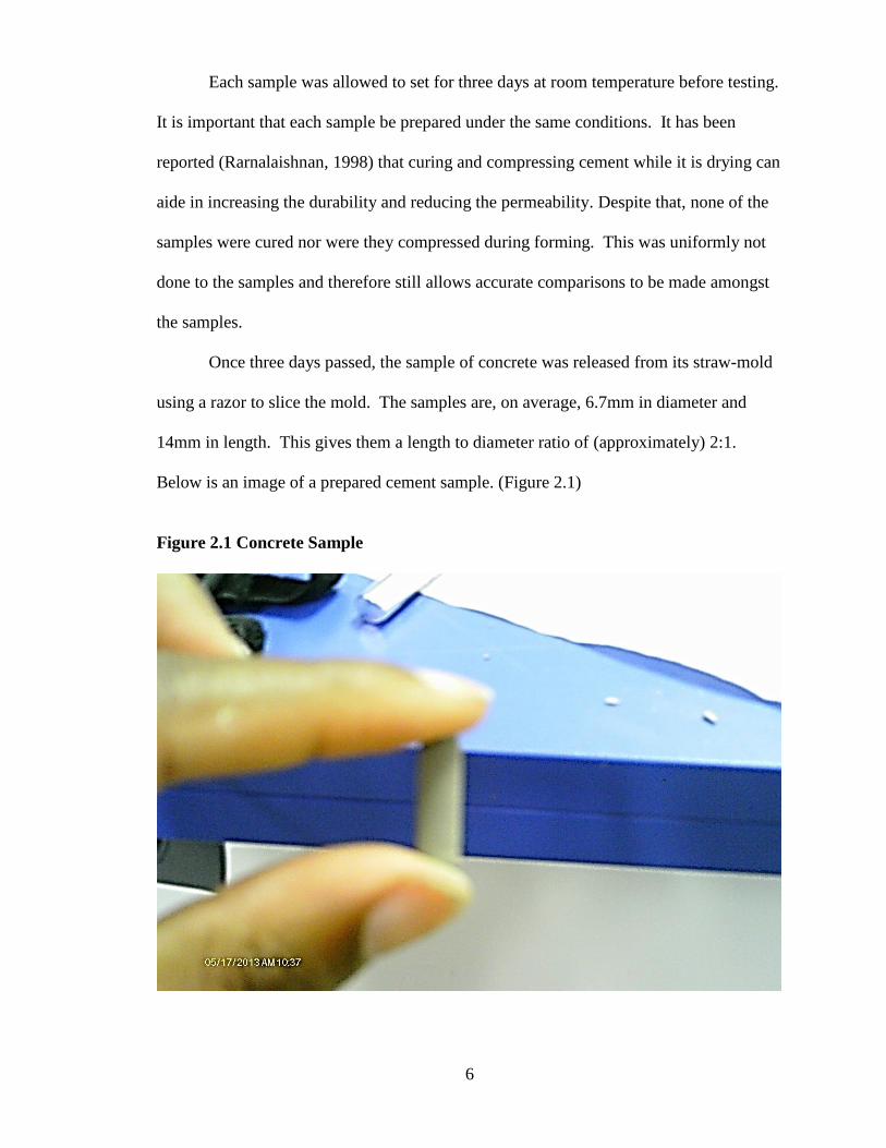
Once three days passed, the sample of concrete was released from its straw-mold

using a razor to slice the mold. The samples are, on average, 6.7mm in diameter and

14mm in length. This gives them a length to diameter ratio of (approximately) 2:1.

Below is an image of a prepared cement sample. (Figure 2.1)

Figure 2.1 Concrete Sample

14 mm

7

Section 2.3 Tools

The tools that were used were: the load frame, the load cell, the LabVIEW

Graphical User Interface, and the Large Chamber Scanning Electron Microscope (LC-

SEM.)

2.3.1 Load Frame

A load frame is machine that is able to test the tensile strength and the

compressive strength of a material. It consists of two strong supports, two platforms, and

a motor that allows one of the platforms to be lowered down towards the fixed platform

as well as raised higher above that same platform. For the purpose of this

experimentation special grips needed to be fabricated from stainless steel in order to hold

the sample with its long axis collinear to the direction of compression. Below is an

image of the steel grip (Figure 2.3a) and the load frame. (Figure 2.3b)

Figure 2.3a Steel Grip Figure 2.3b Load Frame

Load

Cell

Load Frame

8

This load frame is the machine that was used to compress each of the samples of

concrete at a specific rate. The stress rate that is applied from the load frame is varied

and adjusted by the rotations per minute (rpm) of the motor. It is important to note that a

specific rpm of the motor correlates to a certain stress rate that can be reported in

deformation per minute in order to better demonstrate what is physically happening to the

sample. To find the rpm at which the engine must be set to find the desired deformation

rate (x) the form ƒ(x) =𝟕. 𝟒𝟒𝟔𝒙+. 𝟏𝟕𝟑𝟓 is used where x is in micrometers/minute and

the resulting value is in rotations per minute. This is a property of the specific Load

Frame that was used in this experimentation. The equation was found by graphing the

resulting RPMs versus the deformation rate that occurs at that RPM. If the Load Frame

engine is set to a specific RPM, the graphical user interface displays the deformation rate.

Table 1 shows the desired deformation rates and their resulting rotation.

Table 1. Resulting RPMs

Desired Rate (m/min) Resulting RPMs

53.69 400

67.15 500

87.29 650

107.4 800

117.5 875

2.3.2 Load Cell

A load cell is a transducer that is used to convert the applied force into an

electrical signal that can be measured. Below is an image of a load cell. (Figure 2.3)

9

Figure 2.3 Load Cell

For this experimentation, an S-type load cell was used. The force (stress) that is

applied to the load cell deforms a strain gauge within. The deformation changes the

effective electric resistance of the wires that make up the gauge. A load cell is the

standard tool for measuring the stress or strain upon a material being tested by a universal

testing machine (load frame) and it is requisite to the testing process.

10

2.3.3 LabVIEW

The graphical user interface in which the data is read (as well as through which

the Load Frame is controlled) is called Laboratory Virtual Instrument Engineering

Workbench, shorthanded as LabVIEW. This GUI was developed by National

Instuments. Figure 2.4 below shows a screenshot of the LabVIEW interface.

Figure 2.4 LabVIEW Graphical User Interface

The LabVIEW program is often used in industry to allow direct control to

electronic machines during manufacturing of products and in laboritories to control

various mechanical testing devices. It is through this interface that the rotation per

minutes of the Load Frame’s engine can be set (on the compression scale), thereby

setting the deformation rate.

To start the testing

A graph of stress vs deformation

displayed here

To set the deformation

rate

11

This interface also allows the user to take into account the geometry of the sample

(i.e. by allowing the user to input the dimensions of the sample and specify if the sample

is approximately rectangular or more cylindrical in shape). In the present investigation,

the samples were cylindrical (straw-shaped) with an average length of fourteen

millimeters.

In order to begin testing the mouse of the computer is used to click on a white

arrow that is shown on the display of the interface. The arrow turns black to show that

the interface is ready to accept further commands. At this point you are able to enter the

dimensions of the sample. Once set, the button marked “manual” must be clicked. This

button will become illuminated to show that the interface is in manual mode. Manual

mode is necessary so that the RPMs of the Load Frame can be controlled by the user.

Afterwards, clicking on the “Run” button begins the testing. Immediately after the

testing begins, the user must slide the “compression” slider up to the desired rate of

RPMs. It is important that the RPMs be set after the “Run” button is clicked in order to

allow the Load Frame time to ramp up to the desired rate without causing the motor

distress. As a test is run, the GUI gathers data once every half a second. The data

gathered is the following: the time (in seconds), the load of the sample (in Newtons), the

stress on the sample (in MPa), the position of the Load Frame’s motor (in revolutions),

the total amount that the sample has been deformed (in micrometers), the deformation

rate (in micrometers/min), and the Rotations per Minute of the motor of the Load Frame.

The data that is gathered by the user interface is instantly saved onto the hard drive of the

computer in a text file which can later be exported into an Microsoft Excel spreadsheet.

Due to the nature of the machine, tension values ( if the machine is pulling

something apart) are recorded on the GUI interface as positive, whereas compression

12

values (if the machine is pushing something together as in the case of this

experimentation) are recorded as negative. Therefore, when the values are exported into

Microsoft Excel, all of the deformation and stress values are displayed as negative. It is

important that the absolute value of these numbers once they are exported into Excel in

order to show the correct (positive) values.

2.3.4 Scanning Electron Microscope

A scanning electron microscope (SEM) has abilities beyond the capabilities of a

standard optical microscope when it comes to the realm of resolution and depth of field.

Resolution is traditionally defined in microscopy as the ability of the microscope

to produce separate images of closely placed objects (Mann, et. al. 1992). Because

resolution is determined by the wavelength of the image source (half the wavelength of

visible light for an optical microscope or half the wavelength of an electron for an SEM)

a scanning electron microscope can resolve things of a smaller size. More accurately

stated the smallest size of an object (or space between objects) that can be resolved by an

optical microscope is defined by the form d = / (2nsin where: d is the resolvable

feature size, is the wavelength of light, n is the index of refraction of the medium that

the object is being imaged in, and is the half-angle subtended by the objective optical

lens. Given the wavelength of visible light (between 400nm and 700nm), the smallest

resolution size possible under perfect situations would be approximately 200nm. The

wavelength of an electron in a 10 kiloelectronvolt SEM is 12.2pm (12.2x10-12 meters).

Though it, of course is not possible to reach a resolution of have of this wavelength, it is

easy to see that the electron (the image source in an SEM) is able to resolve smaller

objects or distances between objects. The greater resolution (being able to resolve

smaller objects) is desirable due to the small diameter of the basalt fibres that are added

13

to the concrete in this experimentation. To image the sample, the Large Chamber

Scanning Electron Microscope (LC-SEM) used in this experimentation uses backscatter

electrons (BSE). This consists of electrons in an energy beam being fired towards the

sample (Russell, 1985). These electrons are scattered back away from the sample by

elastic scattering interactions with the atoms of the specimen. Be aware that heavier

elements will scatter the electrons back more strongly and therefore appear brighter (than

lighter elements) in the final image. It is important to note that due to the

nonconductivity of cement, during the imaging of the samples the LC-SEM runs in

variable pressure (VP) mode. This allows the LC-SEM to vent a small amount of gas

(atmosphere) into the imaging chamber which reduces/eliminates the charge that would

build up on the surface of a nonconducting sample in a complete vacuum. Figure 2.5

below shows an image of the inside of the Large Chamber Scanning Electron

Microscope.

Figure 2.5 Large Chamber Scanning Electron Microscope

14

In this experimentation, the LC-SEM was used to image the cement samples both

before and after they had gone through the testing procedure. This was done to examine

the interaction that the fibres are having with the cement at its surface and possibly

answer questions such as: do the fibres bind to the cement itself, and do the fibres keep a

certain orientation within the cement? The LC-SEM aides in the interrogation of the

samples to answers the questions and theses answers are compared to the graphs given by

the Load Frame and Load Cell. Figure 2.6 shows a piece of cement with basalt fibres in

it as imaged by the LC-SEM at the NOVA Center at Western Kentucky University, while

Figure 2.7 shows the same sample imaged with a standard optical microscope.

Figure 2.6 Basalt Fibres in Cement at 349x Magnification

15

Figure 2.7 Optical Microscope Image

In image 2.6, the usage of backscattered electrons to image the sample allows not

only an investigation of the surface of the sample, it allows it to be seen that the surface is

not one continuous material, it is a composition created of different materials. As can be

seen, the SEM has the ability to examine the fibres as they move through and out of the

cement, whereas the optical image shows only a fibre as it protrudes out of the cement

sample. The optical image gives us no additional information about how the fibre is

interacting with the cement. However, note the cracks that can be seen (in the SEM

image) in the cement. It is important to this experimentation to verify if the basalt fibres

are bridging the cracks that are in the cement as this will speak to the fibre’s ability to

strength or perhaps weaken the cement structure. If the fibres are creating the cracks, the

graphs that are created by the other instruments will show a decline in strength. If the

16

fibres are bridging the cracks, the graphs created by the other instruments may show an

increase in strength.

Section 2.4 Basalt and Basalt Fibres

Basalt, by definition, is an aphanitic igneous rock with no more than 10%

feldspathoid and no more than 20% quartz by volume. The definition also requires that at

least 65% of the feldspar is in the form of plagioclase (Ozerov 2000.) It is black or grey

in color. Figure 2.8 below shows an image of a basalt rock.

Figure 2.8 Basalt rock (Wikipedia image)

The rock is formed as molten lava cools at or very near the surface of the planet.

Due to the rapid rate of cooling, no crystals are formed within its structure. This rapid

cooling also contributes to its fine-grained texture (Hofmann 2003.)

There are at least five variants of basalt differentiated by additional elements or

minerals that are present in a greater or lesser abundance. The types are: Boninite, Mid

Ocean Ridge, tholeiitic, High alumina, and alkali. It is important to note that any or all of

http://www.google.com/url?sa=i&rct=j&q=&esrc=s&source=images&cd=&docid=2NtGD8rsmqTPnM&tbnid=_xlSz1uyd4CA5M:&ved=0CAUQjRw&url=http://en.wikipedia.org/wiki/Basalt&ei=pRMBU-CJOem0yAH_6IGIAg&bvm=bv.61535280,d.aWc&psig=AFQjCNHdFQorEViKsgHZEzYvJ3V0S5dXmw&ust=1392665517582330

17

the varieties of basalt can be used in the creation of basalt fibres. For the purpose of this

experimentation the basalt fibres were formed from a combination of all basalts.

The transformation of from rock to fibre requires the addition of no additional

material (Ablesimov, et. al 2010.) The rock is washed and crushed, then melted. The

melted basalt is squeezed through thin nozzles to create fibres with a diameter between

9m and 13m. The process is considered “simpler” to manufacture than fibres created

out of glass, despite the higher temperature that is required to melt the basalt rock at

about 1,400°C. For the purpose of this experimentations, the basalt fibres were received

from TFP, a company that specializes in creating mats of non-woven fibres. Below is a

table showing the known properties of basalt fibres.

Table 2. Properties of Basalt Fibres

Property Value

Density (𝒈

𝒄𝒎𝟑) 2.7

Elastic Modulus (GPa) 88

Tensile Strength (GPa) 4.8

Strain at break (%) 3.15

Areal Weight (g/m3) 65

The elastic modulus is a measure of an object’s tendency to be deformed and still

return to its original shape when a force is applied to it (Beer, et. al 2009). Simply stated,

the greater a substance’s elastic modulus, the stiffer the material is. Compare it to the

elastic modulus of steel, which is approximately 200 GPa (2012).

18

The tensile strength of basalt fibres is one of the many properties that makes it a

desirable material. It is defined as the maximum stress that a material can withstand

before failing or breaking (Koler et. al 1995).

Strain at break describes the percentage of the total length that a sample can be

stretched before the sample fails or breaks. It is often written as L/L where L is the total

length of the sample. This value is a portion of the total length and therefore it will be

reported as a percentage in this experimentation instead of a unitless value. The strain at

break is one of the important results of this experimentation.

Another value, the areal weight, speaks to the weight of a specific unit of area of

the fibre when it was in the form of a mat (as it was originally received.)

19

CHAPTER 3 RESULTS

The results of this process of adding fibres is that as the concentration of fibres

added to the cement mixture is increased, the mechanical strength of the cement

decreases. This means that it requires less time at any given pressure to cause the cement

sample to fail and further means that the strain at fail becomes reduced as the fibres are

added to the cement mix.

Section 3.1 Tests at 53.7 m/min

Setting the motor of the Load Frame at 400 rotations per minute via the LabVIEW

interface creates a deformation rate of 53.7 micrometers per minute. The deformation

rate refers to the rate at which the sample is compressed.

For each combination (concentration at stress rate) five tests were completed and

the average of these tests found. It is from the average that graphs of stress versus strain

were formed. A total of four averaged graphs were created for the deformation rate of

53.7 m/min. Graphs 3.1 through 3.4 show the averaged tests.

Graph 3.1 Stress vs. Strain 0% Concentration

0

2

4

6

8

10

12

0 0.5 1 1.5 2 2.5 3 3.5 4 4.5 5

Stre

ss (

MP

a)

Strain (%)

stress vs Strain (No fibres)

20

Graph 3.2 Stress vs. Strain Fibres added at .06% Concentration



0

2

4

6

8

10

12

14

16

0 1 2 3 4 5 6 7 8

stre

ss (

MP

a)

Strain (%)

STRESS VS STRAIN .06% CONCENTRATION

0

2

4

6

8

10

12

0 0.5 1 1.5 2 2.5 3 3.5 4

Stre

ss (

MP

a)

Strain (%)

Stress vs Strain .2% concentration

21

The pertinent data in these graphs is the amount of stress that is on the sample,

measured by the load frame at the time of fail (i.e. the highest stress that the sample

reaches) and the strain of the sample at the time of fail. With these four graphs, it can be

seen that the sample is able to strain less without breaking as the concentration of fibres

increases. Table 3.1 below shows the stress at fail as well as the strain at fail for each of

the concentrations of basalt fibres.

Table 3 Pertinent Information for Tests at Deformation Rate of 53.7 m/min

Concentration of fibres Stress at fail Strain at fail

No fibres 12.32 MPa 4.34%

.06% by mass (of cement) 15.74 MPa 5.43%



0

2

4

6

8

10

12

0 0.5 1 1.5 2 2.5 3 3.5 4 4.5 5

Stre

ss (

MP

a)

Strain (%)


22










0

2

4

6

8

10

12

14

16

0 1 2 3 4 5

Stre

ss (

MP

a)

Strain (%)

Stress vs Strain no fibre added

23

Graph 3.6 Stress vs. Strain Fibres Added at .06% Concentration


0

1

2

3

4

5

6

7

8

9

10

0 0.5 1 1.5 2 2.5 3 3.5

Stre

ss M

Pa

Strain (%)


0

2

4

6

8

10

12

14

0 0.5 1 1.5 2 2.5 3 3.5 4

Stre

ss(M

Pa)

Strain (%)

Stress vs Strain .2% Conentration

24














0

2

4

6

8

10

12

0 0.5 1 1.5 2 2.5 3 3.5 4

Stre

ss (

MP

a)

Stress (%)

Stress vs Stain .8% concentration

25









Graph 3.9 Stress vs Strain 0% Concentration

0

2

4

6

8

10

12

0 1 2 3 4 5 6 7 8

Stre

ss (

MP

a)

Strain(%)

Stress vs Stain No fibres

26

Graph 3.10 Stress vs Strain Fibres added at .06% Concentration


0

1

2

3

4

5

6

7

8

0 0.5 1 1.5 2 2.5 3 3.5 4

Stre

ss (

MP

a)

Strain(%)

stress vs strain .06% concentration

0

2

4

6

8

10

12

0 0.5 1 1.5 2 2.5 3 3.5

Stre

ss(M

Pa)

Strain (%))


27














0

2

4

6

8

10

12

14

0 1 2 3 4 5 6

Stre

ss (

MP

a)

Strain(%)

Stress vs Strain .8% Concentration

28



interface creates a deformation rate of107.4 micrometers per minute. The deformation







0

2

4

6

8

10

12

0 0.5 1 1.5 2 2.5 3 3.5 4 4.5 5

Stre

ss(M

Pa)

Strain(%)

Stress vs Strain no fibres

29

Graph 3.14 Stress vs Strain Fibres Added at .06% Concentration


0

1

2

3

4

5

6

7

8

9

10

0 1 2 3 4 5 6 7

Stre

ss (

MP

a)

Strain (%)

stress vs time .06% Concentration

0

2

4

6

8

10

0 0.5 1 1.5 2 2.5 3 3.5 4 4.5 5

Stre

ss(M

Pa)

Strain(%)


30














0

1

2

3

4

5

6

7

8

0 0.5 1 1.5 2 2.5 3 3.5 4 4.5 5

Stre

ss (

MP

a)

Strain(%)


31









Graph 3.17 Stress vs Strain 0% Concentration

0

2

4

6

8

10

12

0 1 2 3 4 5 6

Stre

ss (

MP

a)

Strain(%)

stress vs strain no fibres added

32

Graph 3.18 Stress vs Strain with Fibres Added at .06% Concentration

Graph 3.19 Stress vs Strain with Fibres added at .2% Concentration

0

2

4

6

8

10

0 1 2 3 4 5 6 7

Stre

ss(M

Pa)

Strain(%)

Stress vs Strain Fibres .06% Concentration

0

2

4

6

8

10

12

14

0 0.5 1 1.5 2 2.5 3 3.5 4

Stre

ss(M

Pa)

Strain(%)


33

Graph 3.20 Stress vs Strain with Fibres Added at .8% Concentration

The important data in these graphs is the amount of stress that is on the sample,


reaches) and the strain of the sample at the time of fail. Table 3.5 below shows the stress

at fail as well as the strain at fail for each of the concentrations of basalt fibres.

Table 7 Information for Tests at Deformation Rate of 117.5 m/min






0

2

4

6

8

10

12

0 1 2 3 4 5 6

Stre

ss (

MP

a)

Strain (%)


34

CHAPTER 4 CONCLUSION

Graph 4.1 below shows how the strain at fail changes as the concentration of

fibres increases. The dashed line is the trendline that represents the exponential decay of

the strain as a function of the concentration of fibres.

Graph 4.1 Stress and Strain vs Concentration (53.7 micro-m/min)

From graph 4.1 it can be seen that adding fibres to the cement mix begins to have

a negative effect on both the durability of the cement (referring to the stress at fail) and

the compressive strength of the cement (referring to the stain at fail) at or beyond a

concentration of 0.2 percent by mass of the cement.

Graph 4.2 below shows how the strain at fail changes as the concentration of

fibres increases.

y = 4.5533e-0.683x

0

1

2

3

4

5

6

0 0.1 0.2 0.3 0.4 0.5 0.6 0.7 0.8 0.9

Stra

in (

%)

Concentration (%)

Strain at Fail vs. Concentration

35

Graph 4.2 Strain at fail vs. Concentration (67.2 micro-m/min)

At a deformation rate of 67.2 micrometers per minute there is a reduction in both

the durability and compressive strength of the cement sample with the addition of fibres

at even the lowest concentration (.06%).

Graph 4.3 below shows how the stress at fail as well as the strain at fail changes

as the concentration of fibres increases.

Graph 4.3 Strain at fail vs concentration (87.3 micro-m/min)

y = 3.3443e-0.498x

0

0.5

1

1.5

2

2.5

3

3.5

4

0 0.1 0.2 0.3 0.4 0.5 0.6 0.7 0.8 0.9

Stra

in (

%)

Concentration (%)


y = 4.3889e-0.099x

0

1

2

3

4

5

6

7

0 0.1 0.2 0.3 0.4 0.5 0.6 0.7 0.8 0.9

Stra

in (

%)

Concentration (%)


36

After an initial dip in the durability of the cement (from 12.80 MPa to 8.28 MPa)

from the test of the cement with no fibres to the test with fibres added at a concentration

of .06% respectively there is an increase in the durability of the cement sample to 13.13

MPa. It is interesting to note that at a concentration of .8% fibres added the stress at fail

is 12.60 MPa, a decline of .20 MPa. This is the smallest decrease that was measured

between a sample with no fibres and a sample with .8% concentration added.

Graph 4.4 below shows how the stress at fail as well as the strain at fail changes as the

concentration of fibres increases.

Graph 4.4 Strain at fail vs concentration (107.4 micro-m/min)

At a concentration of .06% fibres the strain at break is 1.11% greater than it is

when know fibres are added to the sample. Yet at the same concentration the Stress at

time to fail has decreased by 3.04 MPa. A possible explanation for this anomalous

reading is that the samples that were tested at the .06% concentration had a structural

y = 4.9648e-1.189x

0

1

2

3

4

5

6

0 0.1 0.2 0.3 0.4 0.5 0.6 0.7 0.8 0.9

Stra

in (

%)

Concentration (%)


37

flaw that though it allowed the sample to be compressed more without failing also

weakened the structure. An example of such a flaw would be a void in the straw shape of

the sample (such an air bubble in the middle of the sample.)

Graph 4.5 below shows how the stress at fail as well as the strain at fail changes

as the concentration of fibres increases.

Graph 4.5 Strain at fail vs Concentration (117.5 micro-m/min)

At this rate of deformation neither the stress at fail nor the strain at fail decreases

as much as is experienced at other deformation rates. The stress at fail decreased by .37

MPa and the strain at fail decreased by 1.39%.

To make a comparison among the behaviours of each of the stress rates at a given

concentration of fibres added, a graph was made. See graph 4.6 below. On the graph, the

data taken at 400rpms is represented by a blue dash, the data taken at 500rpms is

represented by a black dot, the data taken at 650 rpms is represented by a purple triangle,

the data taken at 800rpms is represented by a light purple square, and the data taken at

y = 5.1407e-0.335x

0

1

2

3

4

5

6

0 0.1 0.2 0.3 0.4 0.5 0.6 0.7 0.8 0.9

Stra

in (

%)

Concentration (%)


38

875rpms is represented by a red diamond. Each trendline formed by the data points has a

color that corresponds to the data.

Figure 4.6 Comparison Graph

The comparison graph shows that though the fibres do lessen the mechanical

strength of the cement sample the amount lessened (at a given concentration) does not

depend on the rate at which the sample is compressed.

An additional comparison that shows the exponential decay as a function of the

rate of deformation (stress rate) is also important to the results of this experimentation.

See graph 4.7 below. This comparison shows how much more (or less) quickly the fibres

cause the sample to fail at any given stress rate. From this it can be seen that there is no

correlation between the stress rate and how the samples will fail. However, it can also be

seen that a higher concentration of fibres reduces the amount of time that it takes for the

sample to fail.

1

2

3

4

5

6

7

0 0.2 0.4 0.6 0.8

Stra

in a

t Fa

il (%

)

Concentration (%)


400RPMs

500RPMs

650RPMs

800RPMs

875RPMs

Expon. (400RPMs)

Expon. (500RPMs)

Expon. (650RPMs)

Expon. (800RPMs)

Expon. (875RPMs)

39

4.7 Decay Rate as a Function of Stress Rate

The practical applications of strengthening concrete are manifold and therefore

experiments such as this that explore cement are beneficial important. Though, the

overall result is that the samples were weakened by the addition of the basalt fibres, it

lends to the full understanding of cement/concrete.

Shown in some of the experiments (such as the experimentation at 53.7

micrometer/min deformation rate) is a slight increase in the stress at fail as well as the

strain at fail at a concentration of .06% fibres. Further experimentation is required to

determine the exact concentration at which the fibres begin to hinder the concrete.

It is very important to note that the sample sized used in testing for this

experimentation produces results that although they speak to results for cement and

concrete in general, cannot be used to unequivocally speak to results for larger samples

(i.e., samples that are longer or have a larger diameter.)

Past experiments (Ramakrishnan et. al. 1998) have shown that it IS possible to

strengthen concrete using basalt fibres. It, then, may be concluded that there is minimum

y = 0.5007e-3E-04x

0

0.2

0.4

0.6

0.8

1

1.2

400 500 600 700 800

Dec

ay r

ate

(tim

e to

fai

l vs

con

cen

trai

tio

n)

Stress Rate (RPMs)

Decay rate versus Stress Rate

40

size (by volume) of the cement/concrete sample at which adding the fibres is beneficial.

This minimum size may be set by the size of the basalt fibres themselves, as they have a

specific diameter that is set at the creation of the fibre.

41

REFERENCES

1"Load cell testing gets straight to the point". Maritime Journal (Mercator Media). 20

December 2010. 2"Wheatstone Bridge Diagrams and Equations". Transducer Techniques.

3"Using the LabVIEW Run-Time Engine". National Instruments.

4Schroettner, H., Schmied, M., & Scherer, S. (2006). Comparison of 3d Surface

Reconstruction Data from Certified Depth Standards Obtained by SEM and an Infinite

Focus Measurement Machine (ifm). Microchim Acta, 155. 279-284.

doi: 10.1007/s00604-006-0556-3

5http://ftp.dot.state.tx.us/pub/txdot-info/cst/tips/frc_4550.pdf

6A. W. Hofmann, Sampling mantle heterogeneity through oceanic basalts: isotopes and

trace elements. Treatise on Geochemistry Volume 2, pages 61–101 Elsevier Ltd. (2003).

ISBN 0-08-044337-0

7A. Y. Ozerov, The evolution of high-alumina basalts of the Klyuchevskoy volcano,

Kamchatka, Russia, based on microprobe analyses of mineral inclusions. Journal of

Volcanology and Geothermal Research, v. 95, pp. 65–79 (2000).

8http://en.wikipedia.org/wiki/Basalt image.

9Ablesimov N.E., Zemtsov A.N. Relaxation effects in non-equilibrium condense systems.

Basalts: from eruption up to a Fibre. (2010). Moskow

10Belov, E.B.e.a. Modeling of permeability of textile reinforcements: Lattice Boltzman

method. in Composites for the future - 10th European Conference on Composite

Materials. 2002. Brugge, Belgium.

11Beer, Ferdinand P.; Johnston, E. Russell; Dewolf, John; Mazurek, David (2009).

Mechanics of Materials. McGraw Hill. p. 56.

12Claridge, Amanda (1998). Rome. Oxford Archaeological Guides. Oxford Oxfordshire:

Oxford University Press

13"Elastic Properties and Young Modulus for some Materials". The Engineering

ToolBox. Retrieved 2012-01-06.

14Köhler, T., Vollrath, F. (1995). "Thread biomechanics in the two orb-weaving spiders

Araneus diadematus (Araneae, Araneidae) and Uloboris walckenaerius (Araneae,

Uloboridae)". Journal of Experimental Zoology 271: 1–17

15Mann, M. J., Espinoza, E. O., & Scanlan, M. D. (1992). Firearms Examinations by

Scanning Electron Microscopy; Observations and an Update on Current and Future

Approaches. AFTE Journal, 24(3), 294-303.

http://www.maritimejournal.com/features101/vessel-build-and-maintenance/monitoring-and-control/load-cell-testing-gets-straight-to-the-point

http://www.transducertechniques.com/wheatstone-bridge.aspx

http://zone.ni.com/reference/en-XX/help/371361B-01/lvhowto/using_the_lv_run_time_eng/

http://ftp.dot.state.tx.us/pub/txdot-info/cst/tips/frc_4550.pdf

http://en.wikipedia.org/wiki/Special:BookSources/0080443370

http://en.wikipedia.org/wiki/Basalt

http://www.engineeringtoolbox.com/young-modulus-d_417.html

42

16Rarnalaishnan, V., Tolmare, N.S. (1998). “Performance Evaluation of 3D Basalt Fibre

Reinforced Concrete & Basalt Rod Reinforced Concrete”. South Dakota School of Mines

& Technology.

17"A Brief History of the University of Illinois". Retrieved May 26, 2011.

18Coumes, Céline Cau Dit; Simone Courtois, Didier Nectoux, Stéphanie Leclercq, Xavier

Bourbon (December 2006). "Formulating a low-alkalinity, high-resistance and low-heat

concrete for radioactive waste repositories". Cement and Concrete Research (Elsevier

Ltd.) 36 (12): 2152–2163

19Kosmatka, S.H.; Panarese, W.C. (1988). Design and Control of Concrete Mixtures.

Skokie, IL, USA: Portland Cement Association. pp. 17, 42, 70, 184

20Cowan, Henry (1977). The Master Builders: : A History of Structural and

Environmental Design From Ancient Egypt to the Nineteenth Century. New York: John

Wiley and Sons.

21Russell, S. D.; Daghlian, C. P. (1985). "Scanning electron microscopic observations on

deembedded biological tissue sections: Comparison of different fixatives and embedding

materials". Journal of Electron Microscopy Technique 2 (5): 489–495.

http://www.library.illinois.edu/archives/features/history.php

Investigation of the Addition of Basalt Fibres into Cement

Documents

Transcript of Investigation of the Addition of Basalt Fibres into Cement