materials

Article

Investigation of Strength and Fatigue Life of RubberAsphalt Mixture

Jiang Yuan 1, Songtao Lv 1,* , Xinghai Peng 1, Lingyun You 2 and Milkos Borges Cabrera 1

1 National Engineering Laboratory of Highway Maintenance Technology, Changsha University of Science andTechnology, Changsha 410004, Hunan, China; yj@stu.csust.edu.cn (J.Y.); pengxinghsi@stu.csust.edu.cn (X.P.);combigra2013@gmail.com (M.B.C.)

2 Department of Civil and Environmental Engineering, Michigan Technological University, Houghton,MI 49931-1295, USA; liyou@mtu.edu

* Correspondence: lst@csust.edu.cn

Received: 1 July 2020; Accepted: 23 July 2020; Published: 26 July 2020�����������������

Abstract: Strength and fatigue life are essential parameters of pavement structure design. Toaccurately determine the pavement structure resistance of rubber asphalt mixture, the strength testsat various temperatures, loading rate, and fatigue tests at different stress levels were conducted inthis research. Based on the proposed experiments, the change law of rubber asphalt mixture strengthwith different temperatures and loading rates was revealed. The phenomenological fatigue equationof rubber asphalt mixture was established. The genetic algorithm optimized backpropagation neuralnetwork (GA-BPNN) is highly reliable for optimizing production processes in civil engineering, andit has a remarkable application effect. A GA-BPNN strength and fatigue life prediction model wascreated in this study. The reliability of the prediction model was verified through experiments. Theresults showed that the rubber asphalt mixture strength decreases and increases with the increase oftemperature and loading rate, respectively. The goodness of fit of the rubber asphalt mixture strengthand fatigue life prediction model based on the GA-BPNN could reach 0.989 and 0.998, respectively.The indicators of the fatigue life prediction model are superior to the conventional phenomenologicalfatigue equation model. The GA-BPNN provides an effective method for predicting the rubberasphalt mixture strength and fatigue life, which significantly improves the accuracy of the resistancedesign of the rubber asphalt pavement structure.

Keywords: rubber asphalt mixture; strength; fatigue life; genetic algorithm; back propagationneural network

1. Introduction

Rubber asphalt mixture has excellent fatigue resistance and water stability, which is an excellentchoice for road engineering [1–4]. However, the asphalt pavement is constantly affected byenvironmental temperature changes, vehicle load, and other factors during its service life. Theirregular and repeated changes of strain stress for a long time will cause the gradual weakening ofthe entire pavement structure’s strength. According to the current statistics, many roads do not reachthe design life, and the pavement will produce cracks and other early diseases, which lead to fatiguefracture damage [5–8].

It is necessary to consider the structural design, material design, construction quality control, andother aspects to solve the early damage of asphalt pavement. Most of the design methods of asphaltpavement structures in the world use the mechanics-experience method, which uses mechanicalmethods to calculate the load response of the pavement structure. It uses homogeneous and isotropiclinear elastic mechanics as the mechanical model for structural response calculation [9–13]. The

Materials 2020, 13, 3325; doi:10.3390/ma13153325 www.mdpi.com/journal/materials

Materials 2020, 13, 3325 2 of 20

strength, stiffness, and fatigue parameters are essential parameters in calculating the load responseand establishing the mechanical model, which plays a vital role in the design of the pavementstructure. Strengthening the anti-fatigue design of the asphalt pavement structure can significantlyreduce the damage caused by unreasonable design, extend the service life of asphalt pavement, andimprove the pavement’s service performance. Therefore, the study on the anti-fatigue design of theasphalt pavement structure will make the design of asphalt pavement more practical, more scientific,and reasonable.

Strength is an essential parameter for designing the pavement structure, reflecting theanti-destructive ability of asphalt pavement [14]. Some scholars have studied the impact of rubberparticle size, content, and gradation type on the rubber asphalt mixture strength [15–19]. Rubberasphalt mixture has viscoelastic characteristics. The temperature and loading rate have a significantimpact on its strength. The strength characteristics of rubber asphalt mixtures obtained by usingdifferent test methods have different results due to various stress modes. Furthermore, the phenomenonof the random value of strength parameters in the design of asphalt pavement structure is produced,which leads to an inaccurate calculation of the resistance of the pavement structure. However, thestrength test results directly affect the results of the fatigue test of the rubber asphalt mixture.

The fatigue performance of asphalt mixture is the research hotspot of asphalt pavement. Thefactors that affect the fatigue performance of asphalt mixture mainly include the test method, materialfactor, loading frequency, test temperature, etc. In terms of test methods, indoor tests are primarilyused in the world, including the direct tensile test, indirect tensile test, and four-point bending test.The fatigue test results obtained by different test methods and different specimen sizes are different.In terms of material factors, Li et al. studied the influence of asphalt types and gradation typeson the fatigue performance of asphalt mixtures [20]. They found that Styreneic Block Copolymers(SBS) modified asphalt has the best fatigue performance. Jiang et al. conducted fatigue tests onporous asphalt mixtures composed of different materials [21]. They studied the effects of porosity,asphalt–aggregate ratio, and water immersion on the fatigue characteristics of the asphalt mixture.The results showed that the impact of water immersion on the fatigue characteristics of porous asphaltmixtures is closely related to the asphalt–aggregate ratio. Pell uses sine waves for loading, and thefrequency range is 80–2500 r/min [22]. The results showed that the higher the frequency, the longerthe fatigue life. The test temperature has a significant effect on the fatigue performance of the asphaltmixture. The studies have shown that when using stress control, the lower the temperature, the longerthe fatigue life [23]. When strain control is used, the fatigue life is less dependent on the temperature atlow temperatures. As the temperature increases, the fatigue life increases. In summary, it can be foundthat many factors will affect the fatigue performance of asphalt mixtures, and the fatigue test results area vital factor that determines the accuracy of the fatigue life prediction equation of asphalt mixtures.

Fatigue life is an important basis for studying the anti-fatigue performance of asphalt pavementmaterials. Meanwhile, the fatigue life prediction is a long-lasting topic. There are three methods toforecast the asphalt mixture fatigue life: the dissipation energy method, fracture mechanics method,and phenomenology method [24–28].

There is a part of research on the prediction of asphalt mixture fatigue life according to the principleof dissipated energy [29–33]. According to Van Dijk et al.’s research, fatigue life mainly depends onthe dissipation modulus and energy consumption during the stress–strain cycle [34]. The mechanicalproperties of the asphalt mixture depend on how long the load is applied and the temperature whenthe pressure is applied [35]. Its complex modulus is composed of a storage modulus and loss modulus.The main characteristic of the dissipated energy method is that there is a unique relationship betweenthe cumulative dissipated energy and fatigue life [36,37]. Other factors (e.g., test method, loadingmode) have a negligible effect. In fact, the dissipated energy of each cycle of damage is not constant,due to the accumulation of cracks in the mixture samples while conducting the asphalt mixture fatiguetest, but it gradually increases with the increase of cycle times. Therefore, using a dissipated energymethod to predict the fatigue life will cause higher errors in practical applications.

Materials 2020, 13, 3325 3 of 20

The fracture mechanics method predicts the fatigue life of asphalt mixtures, according to P.C.Paris’ crack growth formula [38]. Fracture mechanics divides the fatigue failure process into the crackinitiation and crack propagation stage [39]. It is a continuous process from the formation of the fatiguecrack to the propagation of the crack. The initial crack will be produced after the asphalt mixturehas experienced a long fatigue process, which means that the initiation life of a fatigue crack is verylong [40]. However, the life of this stage is ignored in fracture mechanics. Therefore, it is unreasonableto adopt the fracture mechanics method to predict the asphalt mixture fatigue life.

The phenomenological method is a common way for predicting the fatigue life of asphaltmixtures [41]. The fatigue equations are obtained by fitting the fatigue test curves under different strainor stress levels. The asphalt mixtures’ fatigue life under different strain or stress levels is estimated byusing this equation [42]. However, there is some discreteness in the estimated equation. Thus, it isparticularly important to predict the fatigue life of asphalt mixtures accurately.

Meanwhile, many scholars have done numerous research studies in data prediction. Thebackpropagation neural network (BPNN) is one of the commonly used methods for data prediction.The BPNN has the ability of robust nonlinear mapping and has been widely used in civil engineering.Abdelkader et al. used BPNN to predict cement concrete’s compressive strength [43]. Kheradmandiet al. proposed to use the BP method to calculate the interlayer modulus [44]. Besides, the fatiguelife and optimum asphalt content also can be predicted with the BPNN model. Xiao et al. usedregression analysis and neural network methods to forecast the recycled rubber asphalt mixture’ fatiguelife [45]. Although the BP NN has achieved many outstanding results in the field of civil engineering,it takes a long time to approximate the predicted value, resulting in a slow convergence speed ofthe network. On the other hand, there are few studies on the application of BPNN in the rubberasphalt mixture’s strength and fatigue properties. However, the genetic algorithm (GA) has betterglobal searchability, and it can obtain the optimal global solution with faster convergence speed [46].Therefore, to improve the optimization ability of the BPNN and reduce the possibility that BPNN fallsinto a local optimization, the GA-BPNN model by using GA optimization on a BPNN is established.Considering the above reasons, GA-BPNN will be used to forecast the strength and fatigue life ofrubber asphalt mixture in this research.

In summary, the accurate prediction of the rubber asphalt mixture strength and fatigue life isessential for ensuring the scientific and reasonable anti-fatigue design of rubber asphalt pavementstructures. Based on this, in this study, the change rule of the strength of rubber asphalt mixtureswith different temperatures and loading rates is revealed. The fatigue test is conducted at differentstress levels. The conventional phenomenological fatigue equation of a rubber asphalt mixture isestablished. The prediction model of rubber asphalt mixture strength and fatigue life is created basedon a genetic algorithm optimized backpropagation neural network (GA-BPNN). The goodness of fit ofthe fatigue life prediction model is compared with that one of the conventional phenomenologicalfatigue equation models. In addition to the training data, the strength and fatigue tests are carried outto verify the feasibility of the model.

2. Methods

2.1. GA-BPNN

BPNN is a kind of neural network algorithm based on error backpropagation [47]. Its trainingprocess is repeated alternately by forwarding propagation and backpropagation. The input, hidden,and output layers constitute the basic structure of the BPNN. Its basic structure is shown in Figure 1.X1, X2, . . . , Xm are the input values. Y1, Y2, . . . , Ym are the output values.

Materials 2020, 13, 3325 4 of 20Materials 2020, 13, x FOR PEER REVIEW 4 of 21

X1

X2

Xm

Y2

Ym

Y1

..

....

Input layer Hidden layer Output layer

Figure 1. Backpropagation neural network (BPNN) structure.

GA is a computational model simulating the natural selection and genetic mechanism of Darwinian biological evolution [48]. The pattern theorem reveals the mechanism of GA., which is the main theorem of the genetic algorithm. The procedure is as follows.

Assuming that at a given time step t, a particular pattern H has m representative strings contained in population ( )A t , which is recorded as ( ),m m H t= . During the regeneration stage,

the fitness of an individual iA is if , and each string replicates according to its fitness value. The

regeneration probability of a string iA is:

1

n

i i ii

P f f=

= .

(1)

When non-overlapping n string populations are used instead of populations ( )A t , the

following formula can be obtained:

( ) ( ) ( )1

, 1 ,n

ii

m H t m H t n f H f=

+ = (2)

where ( )f H is the average fitness of the string of pattern H in time t. The average fitness of the

whole population can be recorded as:

n

ii

f f n=. (3)

Under the structural conditions of the basic GA, if the genetic operation only chooses to transfer to the next generation, the following formula holds:

( ) ( ) ( ), 1 ,m H t m H t f H f+ =. (4)

Equation (4) shows that a particular pattern grows according to the ratio between its average fitness value and the population’s average fitness value. Suppose that from 0t = , the fitness value

Figure 1. Backpropagation neural network (BPNN) structure.

GA is a computational model simulating the natural selection and genetic mechanism of Darwinianbiological evolution [48]. The pattern theorem reveals the mechanism of GA., which is the maintheorem of the genetic algorithm. The procedure is as follows.

Assuming that at a given time step t, a particular pattern H has m representative strings containedin population A(t), which is recorded as m = m(H, t). During the regeneration stage, the fitness of anindividual Ai is fi, and each string replicates according to its fitness value. The regeneration probabilityof a string Ai is:

Pi = fi/n∑

i=1

fi . (1)

When non-overlapping n string populations are used instead of populations A(t), the followingformula can be obtained:

m(H, t + 1) = m(H, t)n f (H)/n∑

i=1

fi (2)

where f (H) is the average fitness of the string of pattern H in time t. The average fitness of the wholepopulation can be recorded as:

f =n∑i

fi/n . (3)

Under the structural conditions of the basic GA, if the genetic operation only chooses to transferto the next generation, the following formula holds:

m(H, t + 1) = m(H, t) f (H)/ f . (4)

Equation (4) shows that a particular pattern grows according to the ratio between its averagefitness value and the population’s average fitness value. Suppose that from t = 0, the fitness value of acertain pattern is more than c f above the average fitness value of the population, and c is a constant.Then, the pattern selection growth equation becomes:

m(H, t + 1) = m(H, t)f(

f + c f)

f= (1 + c) ·m(H, t) = (1 + c)t

·m(H, 0). (5)

Materials 2020, 13, 3325 5 of 20

Under simple crossover, the probability of the general pattern H being destroyed isPd = δ(H)/(t− 1), and the survival probability is Ps = 1 − δ(H)/(t− 1). The crossover itself occurswith a certain probability Pc, so the survival probability of pattern H is calculated as follows:

Ps = 1− PcPd = 1− Pc · δ(H)/(t− 1). (6)

At the same time, considering the influence of selection and crossover operations on the pattern,an estimate of the sub generation pattern can be obtained:

m(H, t + 1) ≥ m(H, t) ·f (H)

f·

[1− Pc

δ(H)

t− 1

]. (7)

Suppose that the probability of a certain position of the string changing is Pm; then, the probabilitythat the position is unchanged is 1− Pm. The probability of pattern H being invariable is (1− Pm)

o(H),where o(H) is the order of pattern H. The survival probability of pattern H under the action of mutationoperator is:

Ps = (1− Pm)o(H)≈ 1− o(H)Pm. (8)

In summary, under the combined effect of genetic operator selection, crossover, and mutation, thenumber of samples of its offspring of pattern H are:

m(H, t + 1) ≥ m(H, t) ·f (H)

f·

[1− Pc

δ(H)

t− 1

]· [1− o(H)Pm]. (9)

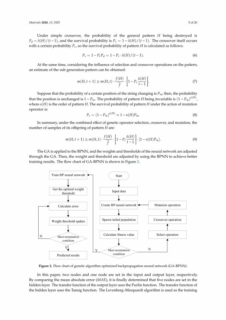
The GA is applied to the BPNN, and the weights and thresholds of the neural network are adjustedthrough the GA. Then, the weight and threshold are adjusted by using the BPNN to achieve bettertraining results. The flow chart of GA-BPNN is shown in Figure 2.

Materials 2020, 13, x FOR PEER REVIEW 6 of 21

Train BP neural network

Get the optimal weight threshold

Calculate error

Weight threshold update

Predicted results

Meet termination condition

Start

Input data

Create BP neural network

Spawn initial population

Calculate fitness value

Meet termination condition

Select operation

Crossover operation

Mutation operation

N

Y NY

Figure 2. Flow chart of genetic algorithm optimized backpropagation neural network (GA-BPNN).

In this paper, two nodes and one node are set in the input and output layer, respectively. By comparing the mean absolute error (MAE), it is finally determined that five nodes are set in the hidden layer. The transfer function of the output layer uses the Purlin function. The transfer function of the hidden layer uses the Tansig function. The Levenberg–Marquardt algorithm is used as the training function, which effectively overcomes the shortcomings of the slow convergence of the neural network. The learning rate is 0.5, the number of training steps is 1000, and the learning goal is 0.0001. The optimization parameter, maximum genetic generation, crossover probability, and mutation probability related to GA are equal to 30, 150, 0.6, and 0.05, respectively. All neural network simulations are performed on MATLAB R2016b.

2.2. Phenomenological Method

In the phenomenological method, the fatigue strength is the value of the repeated stress at which fatigue failure occurs in a material. The following is the derivation process of the fatigue equation based on the phenomenological method.

Considering the influence of stress amplitude, a common damage evolution model is [49]:

( ) ( )( ) 11 12 2 1

dD D DdN M M D

α α αα γ γσ σ− + − = − = − −

. (10)

Integrating Equation (10) obtains:

( )1

1

1 1f

ND NN

α γ+ + = − −

(11)

where the Nf is the fatigue life, which can be expressed by Equation (12):

( )

( ) ( )1 1 1

1 2 1 2fNM M

α α

ασ

α γ σα γ

−

− = = + + + +

. (12)

Figure 2. Flow chart of genetic algorithm optimized backpropagation neural network (GA-BPNN).

In this paper, two nodes and one node are set in the input and output layer, respectively.By comparing the mean absolute error (MAE), it is finally determined that five nodes are set in thehidden layer. The transfer function of the output layer uses the Purlin function. The transfer function ofthe hidden layer uses the Tansig function. The Levenberg–Marquardt algorithm is used as the training

Materials 2020, 13, 3325 6 of 20

function, which effectively overcomes the shortcomings of the slow convergence of the neural network.The learning rate is 0.5, the number of training steps is 1000, and the learning goal is 0.0001. Theoptimization parameter, maximum genetic generation, crossover probability, and mutation probabilityrelated to GA are equal to 30, 150, 0.6, and 0.05, respectively. All neural network simulations areperformed on MATLAB R2016b.

2.2. Phenomenological Method

In the phenomenological method, the fatigue strength is the value of the repeated stress at whichfatigue failure occurs in a material. The following is the derivation process of the fatigue equationbased on the phenomenological method.

Considering the influence of stress amplitude, a common damage evolution model is [49]:

dDdN

=(σ

2M

)α(1−D)−(α+γ) =

( 12M

)α( σ1−D

)α(1−D)−γ. (10)

Integrating Equation (10) obtains:

D(N) = 1−(1−

NN f

) 11+α+γ

(11)

where the Nf is the fatigue life, which can be expressed by Equation (12):

N f =1

1 + α+ γ

(σ

2M

)(−α)=

1(1 + α+ γ)(2M)−α

(1σ

)α. (12)

Let k = 1(1+α+γ)(2B)−α

, n = α, Equation (12) can be transformed into Equation (13).

N f = k(1σ)

n(13)

Equation (13) can be derived as follows:

lgN f = lgk− nlgσ. (14)

Equation (14) is a conventional phenomenological fatigue equation. Where σ is stress level; D isfatigue damage; N is times of loading actions; N f is fatigue life; and M,α,γ are material parametersto temperature.

3. Experimental

3.1. Materials

3.1.1. Asphalt

In this paper, Donghai brand 70-grade road asphalt was selected as the neat asphalt. The rubberpowder obtained from bias tires was sieved by using 40 mesh. The content of waste tire rubberpowder is 21% of the neat asphalt mass. A small indoor mixer was used to prepare the rubberasphalt. The stirring temperature was set at 185 ◦C, and the stirring time was equal to 60 min. Themain technical indexes of neat asphalt, waste tire rubber powder, and rubber asphalt are shown inTables 1–3, respectively.

Materials 2020, 13, 3325 7 of 20

Table 1. Indexes of neat asphalt.

Index Unit Test Results Technical Requirement

Penetration (25 ◦C, 100 g, 5 s) 0.1 mm 64 60–80Softening point ◦C 48.5 ≥46

Ductility (15 ◦C, 5 cm/min) cm >100 ≥100Density (15 ◦C) g/cm3 1.029 -

Dynamic viscosity (60 ◦C) Pa·s 199.3 ≥180

Table 2. Technical indexes of waste tire rubber powder.

Index Unit Test Results Technical Requirement

Water content % 0.58 <1Metal content % 0.03 <0.05Fiber content % 0.03 <1Ash content % 6 ≤8

Carbon black content % 32 ≥28Rubber hydrocarbon content % 55 ≥42

Table 3. Technical indexes of rubber asphalt.

Index Unit Test Results Technical Requirement

Penetration (25 ◦C, 100 g, 5 s) 0.1 mm 42.0 30–70Softening point ◦C 68.5 ≥65

Ductility (15 ◦C, 5 cm/min) cm 11.6 ≥5Dynamic viscosity (60 ◦C) Pa·s 3.16 1.5–4

Elastic recovery % 87.3 >60

3.1.2. Coarse and Fine Aggregate

Limestone was used for coarse and fine aggregate. The aggregate performance test results areshown in Tables 4 and 5. Limestone mineral powder was used as filler.

Table 4. Test results of aggregate density.

Number Particle SizeSpecification (mm)

Apparent RelativeDensity (g/cm3)

Bulk Volume RelativeDensity (g/cm3)

Water Absorption(%)

1 16–13.2 2.714 2.692 0.312 13.2–9.5 2.719 2.695 0.333 9.5–4.75 2.721 2.689 0.454 4.75–2.36 2.722 2.648 1.035 2.36–1.18 2.761

- -6 1.18–0.6 2.7167 0.6–0.3 2.7268 0.3–0.15 2.7379 0.15–0.075 2.725

Table 5. Mechanical properties of limestone.

Aggregate Type Crush Value (%) Polishing Value (BPN) Abrasion Value (%)

Limestone 15.8 57.4 19.9Technical requirement ≤28 ≥45 ≤30

3.1.3. Grading Design

According to the middle value of ARAC-13 type grading recommended in Shanghai 2012 technicalcode for rubber asphalt pavement, the grading curve in this paper is determined, as shown in Figure 3.

Materials 2020, 13, 3325 8 of 20

The optimum asphalt content of rubber asphalt mixture is determined to be 7.2% by using the Marshalldesign method.Materials 2020, 13, x FOR PEER REVIEW 9 of 21

0.075 0.15 0.3 0.6 1.18 2.3 4.75 9.5 13.2 160

10

20

30

40

50

60

70

80

90

100Pa

ssin

g po

rcen

tage

(%)

Sieve size(mm)

Upper gradation Middle gradation Lower gradation Target gradation

Figure 3. Gradation of the ARAC-13 rubber asphalt mixture.

3.2. Experiment Scheme

To assess the tensile, compression, bending, and shear characteristics of asphalt mixtures, the commonly used methods for indoor strength tests include the direct stretching, uniaxial compression, four-point bending, and indirect stretching methods. There are many methods for fatigue properties testing. The most common test methods used across the world are the indirect tension method, trapezoidal cantilever bending method, and four-point bending method.

Since the center point of the specimen in the indirect tensile test is in transverse tension and longitudinal compression, which is more consistent with the actual stress state of the asphalt pavement structure, the indirect tensile method was selected to study the strength and fatigue properties of rubber asphalt mixture in this research. The cylinder specimen with a diameter of 100 ± 2 mm and a height of 100 ± 2 mm was obtained by using rotary compaction. Then, the cylinder specimen with a diameter of 100 ± 2 mm and a height of 65 ± 2 mm was cut by utilizing a cutting machine. The specimen is shown in Figure 4a.

In this study, the strength and fatigue tests of rubber asphalt mixture are carried out with a MTS-Landmark operating system and the matching temperature control box. The MTS-Landmark operating system can provide different loading rates and stress levels, and the temperature control box can meet the requirements of the test temperature. Figure 4b shows the indirect tensile test.

Figure 3. Gradation of the ARAC-13 rubber asphalt mixture.

3.2. Experiment Scheme

To assess the tensile, compression, bending, and shear characteristics of asphalt mixtures, thecommonly used methods for indoor strength tests include the direct stretching, uniaxial compression,four-point bending, and indirect stretching methods. There are many methods for fatigue propertiestesting. The most common test methods used across the world are the indirect tension method,trapezoidal cantilever bending method, and four-point bending method.

Since the center point of the specimen in the indirect tensile test is in transverse tension andlongitudinal compression, which is more consistent with the actual stress state of the asphalt pavementstructure, the indirect tensile method was selected to study the strength and fatigue properties ofrubber asphalt mixture in this research. The cylinder specimen with a diameter of 100 ± 2 mm and aheight of 100 ± 2 mm was obtained by using rotary compaction. Then, the cylinder specimen witha diameter of 100 ± 2 mm and a height of 65 ± 2 mm was cut by utilizing a cutting machine. Thespecimen is shown in Figure 4a.

In this study, the strength and fatigue tests of rubber asphalt mixture are carried out with aMTS-Landmark operating system and the matching temperature control box. The MTS-Landmarkoperating system can provide different loading rates and stress levels, and the temperature control boxcan meet the requirements of the test temperature. Figure 4b shows the indirect tensile test.

Stress control was adopted in the strength and fatigue test of rubber asphalt mixture. The testtemperatures for strength tests were equal to10 ◦C, 15 ◦C, and 20 ◦C. The loading rates were equalto 0.02 MPa/s, 0.05 MPa/s, 0.1 MPa/s, 0.2 MPa/s, 0.5 MPa/s, 1 MPa/s, and 2 MPa/s. The fatigue testtemperature, the loading frequency, and the loading waveform are 20 ◦C, 10 Hz, and continuouspositive vector waves, respectively.

Materials 2020, 13, 3325 9 of 20

Materials 2020, 13, x FOR PEER REVIEW 10 of 21

(a) (b)

Figure 4. Indirect tensile test specimen and test drawing: (a) Rotary compacted cylindrical specimen; (b) Indirect tensile test chart.

Stress control was adopted in the strength and fatigue test of rubber asphalt mixture. The test temperatures for strength tests were equal to10 °C, 15 °C, and 20 °C. The loading rates were equal to 0.02 MPa/s, 0.05 MPa/s, 0.1 MPa/s, 0.2 MPa/s, 0.5 MPa/s, 1 MPa/s, and 2 MPa/s. The fatigue test temperature, the loading frequency, and the loading waveform are 20 °C, 10 Hz, and continuous positive vector waves, respectively.

4. Results and Discussion

4.1. Analysis of Strength Test Results

According to the experiment scheme, three parallel tests were conducted under the same conditions. The rubber asphalt mixture strength test results under different temperatures and loading rates are shown in Table 6.

Table 6. The rubber asphalt mixture strength results.

Number Temperature (°C)

Loading Rate

(MPa/s)

Strength

(MPa) Mean Value of Strength

(MPa)

Standard Deviations

Sample 1 Sample 2 Sample 3 1

10

0.02 0.520 0.762 0.665 0.649 9.94 2 0.05 0.846 0.811 0.827 0.828 1.43 3 0.1 0.852 1.120 0.863 0.945 12.38 4 0.2 1.429 1.150 1.321 1.300 0.11 5 0.5 1.794 1.512 1.770 1.692 0.13 6 1 1.651 1.881 1.604 1.712 0.12 7 2 2.394 1.984 2.231 2.203 0.17 8

15 0.02 0.516 0.484 0.572 0.524 0.04

9 0.05 0.680 0.662 0.632 0.658 0.02 10 0.1 0.758 0.782 0.923 0.821 0.07

Figure 4. Indirect tensile test specimen and test drawing: (a) Rotary compacted cylindrical specimen;(b) Indirect tensile test chart.

4. Results and Discussion

4.1. Analysis of Strength Test Results

According to the experiment scheme, three parallel tests were conducted under the same conditions.The rubber asphalt mixture strength test results under different temperatures and loading rates areshown in Table 6.

Table 6. The rubber asphalt mixture strength results.

Number Temperature(◦C)

Loading Rate(MPa/s)

Strength (MPa) Mean Value ofStrength (MPa)

StandardDeviationsSample 1 Sample 2 Sample 3

1

10

0.02 0.520 0.762 0.665 0.649 9.942 0.05 0.846 0.811 0.827 0.828 1.433 0.1 0.852 1.120 0.863 0.945 12.384 0.2 1.429 1.150 1.321 1.300 0.115 0.5 1.794 1.512 1.770 1.692 0.136 1 1.651 1.881 1.604 1.712 0.127 2 2.394 1.984 2.231 2.203 0.17

8

15

0.02 0.516 0.484 0.572 0.524 0.049 0.05 0.680 0.662 0.632 0.658 0.0210 0.1 0.758 0.782 0.923 0.821 0.0711 0.2 1.044 0.893 0.937 0.958 0.0612 0.5 0.970 1.025 1.200 1.065 0.1013 1 1.512 1.577 1.240 1.443 0.1514 2 1.594 1.346 1.731 1.557 0.16

15

20

0.02 0.447 0.454 0.488 0.463 0.0216 0.05 0.584 0.573 0.589 0.582 0.0117 0.1 0.682 0.633 0.707 0.674 0.0318 0.2 0.845 0.713 0.740 0.766 0.0619 0.5 1.016 0.948 0.811 0.925 0.0920 1 1.128 0.939 1.092 1.053 0.0821 2 1.308 1.191 1.212 1.237 0.05

To analyze the influence of different temperatures and loading rates on the rubber asphalt mixturestrength, the test results are presented in Figure 5 with a scatter diagram. It can be observed from

Materials 2020, 13, 3325 10 of 20

Figure 5 that the strength value of rubber asphalt mixture increases with the increase of loading rateregardless of the temperature, and it decreases with the increase of temperature regardless of theloading rate. To better analyze the change rule of the rubber asphalt mixture strength, a nonlinearfitting has been carried out for the loading rate and strength. The fitting equation is as shown inEquation (15). The fitting results are shown in Table 7.

S = α× vβ (15)

where S is the strength value; v is the loading rate; α, β is the fitting parameter.

Materials 2020, 13, x FOR PEER REVIEW 11 of 21

11 0.2 1.044 0.893 0.937 0.958 0.06

12 0.5 0.970 1.025 1.200 1.065 0.10

13 1 1.512 1.577 1.240 1.443 0.15

14 2 1.594 1.346 1.731 1.557 0.16

15

20

0.02 0.447 0.454 0.488 0.463 0.02

16 0.05 0.584 0.573 0.589 0.582 0.01

17 0.1 0.682 0.633 0.707 0.674 0.03

18 0.2 0.845 0.713 0.740 0.766 0.06

19 0.5 1.016 0.948 0.811 0.925 0.09

20 1 1.128 0.939 1.092 1.053 0.08

21 2 1.308 1.191 1.212 1.237 0.05

To analyze the influence of different temperatures and loading rates on the rubber asphalt

mixture strength, the test results are presented in Figure 5 with a scatter diagram. It can be observed

from Figure 5 that the strength value of rubber asphalt mixture increases with the increase of loading

rate regardless of the temperature, and it decreases with the increase of temperature regardless of the

loading rate. To better analyze the change rule of the rubber asphalt mixture strength, a nonlinear

fitting has been carried out for the loading rate and strength. The fitting equation is as shown in

Equation (15). The fitting results are shown in Table 7.

S v (15)

where S is the strength value; v is the loading rate; , is the fitting parameter.

0.0 0.5 1.0 1.5 2.0

0.5

1.0

1.5

2.0

2.5

3.0

3.5

18

18

1716

15

1110

9

8

4

32

21

21

2019

1716

15

1413

1211

109

8

7

65

4

3

0.00 0.05 0.10 0.15 0.20 0.25 0.300.4

0.6

0.8

1.0

1.2

1.4In

dir

ect

ten

sile

str

eng

th /

MP

a

Loading rate / MPa/s

10℃

15℃

20℃

Indir

ect

tensi

le s

tren

gth

/ M

Pa

Loading rate / MPa/s

1

Figure 5. Law of changes related to indirect tensile strength with different loading rates and

temperatures.

The results indicate that there is a good correlation between the indirect tensile strength and the

loading rate at each temperature. It can be noticed from Table 7 that the change rule is consistent

with the change rule of rubber asphalt mixture strength, and both decrease with the increase of

temperature. That is to say, reflects the law of strength change. reflects the sensitivity of the

strength to the loading rate. The larger is, the more sensitive strength is to the loading rate. It can

Figure 5. Law of changes related to indirect tensile strength with different loading ratesand temperatures.

Table 7. Fitting curve equation between indirect tensile strength and loading rate withdifferent temperatures.

Temperature α β R2

10 ◦C 1.83887 0.25600 0.96715 ◦C 1.35319 0.23358 0.97420 ◦C 1.06645 0.20623 0.999

The results indicate that there is a good correlation between the indirect tensile strength and theloading rate at each temperature. It can be noticed from Table 7 that the change rule α is consistent withthe change rule of rubber asphalt mixture strength, and both decrease with the increase of temperature.That is to say, α reflects the law of strength change. β reflects the sensitivity of the strength to theloading rate. The larger β is, the more sensitive strength is to the loading rate. It can be noticed fromthe analysis that while the temperature increases from 10 ◦C to 20 ◦C, β decreases gradually, and thesensitivity of the strength to the loading rate gradually decreases.

On the other hand, as the loading rate increases, the strength value increases; subsequently, itsvariability becomes greater and greater, and it is more susceptible to other factors. Yu et al. conductedthe compressive resilience modulus test at 15 ◦C and 20 ◦C and the splitting strength test at 15 ◦Con three rubber asphalt mixtures [50]. The results showed that the splitting strength of differentgrade rubber asphalt mixtures has a special proportional relationship with the compressive resilience

Materials 2020, 13, 3325 11 of 20

modulus. The difference in the rubber asphalt mixture between the two test temperatures is 0.85 times.Compared with neat asphalt mixtures, rubber asphalt mixtures have higher strength values. The testresults of this research show that under the combined effect of test temperature and loading rate, themaximum strength value of rubber asphalt mixture, 2.203 MPa, is 4.75 times the minimum value,0.463 MPa.

4.2. Establishment of the Strength Prediction Model

The strength test data in Table 6 are processed, which obtain 21 group data required for training.Each set of training data contains 2 input values (temperature, loading rate) and 1 output value (averagestrength value). To increase the training speed, it is also necessary to normalize the data. The MATLABR2016b program was used to build the GA-BPNN structure, as described above. Twenty-one sets oftraining data were used to train the network. There is no specific method for selecting the numberof hidden layer nodes in the BPNN. If the number of hidden layer nodes is too small, it can lead toproblems related to meeting the expected requirements, but too many hidden layer nodes may result ina lengthy training time and “overfitting”. In this study, to improve the accuracy of the model, differentnetwork structures were tried in the hidden layer. According to the general hidden layer determinationmethod, the range of hidden layer nodes was selected from 3 to 13. Then, the number of hidden layernodes was determined by comparing the mean absolute error (MAE), the goodness of fit (R2), and thestandard error of predicted values divided by that of actual values (Se/Sy). The calculation of MAE, R2,and Se/Sy is as shown in Equations (16)–(18). Figure 6a–c reflect the results of the network structurecorresponding to the hidden layer with a different number of nodes. The lower the MAE, the greaterthe R2, the lower the Se/Sy, and the more accurate the prediction model. From Figure 6a–c, it can befound that when the number of hidden neurons is equal to 5, the value of MAE is the smallest; whenthe number of hidden neurons is equal to 5 and 6, the value of R2 is the largest. When the number ofhidden neurons is equal to 5, the value of Se/Sy is the smallest. It can be noticed from Figure 6 thatwhile the number of hidden layer nodes is 5, the GA-BPNN structure achieves its best performance.

MAE =1n

n∑i=1

(∣∣∣Ypre − Yexp∣∣∣ ) (16)

R2 = 1−

n∑i=1

(Ypre(i) −Yexp(i)

)2

n∑i=1

(Ypre(i) −Yexp

)2(17)

Se

Sy=

√√√√√√√√√√√√ n∑i=1

(Yexp(i) −Ypre(i)

)2× n

n∑i=1

(Yexp(i) −Yexp

)2× (n−m)

(18)

where Ypre is the predicted value; Yexp is the experiment value; and n, m are the number of tests andvariables, respectively.

Materials 2020, 13, 3325 12 of 20

Materials 2020, 13, x FOR PEER REVIEW 13 of 21

( )

( )

2

pre( ) exp( )2 1

2

pre( ) exp1

1

n

i ii

n

ii

Y YR

Y Y

=

=

−= −

−

(17)

( )

( ) ( )

2

( ) ( )1

2

( )1

n

exp i pre ie i

ny

exp i expi

Y Y nSS Y Y n m

=

=

− ×=

− × −

(18)

where preY is the predicted value; expY is the experiment value; and n, m are the number of tests and

variables, respectively.

2 4 6 8 10 12 140.01

0.02

0.03

0.04

0.05

0.06

0.07

MAE

Number of hidden neurons (a)

2 4 6 8 10 12 140.5

0.6

0.7

0.8

0.9

1.0

1.1

1.2

R2

Number of hidden neurons (b)

Materials 2020, 13, x FOR PEER REVIEW 14 of 21

2 4 6 8 10 12 140.0

0.1

0.2

0.3

0.4

0.5

0.6

0.7

0.8

S e /

S y

Number of hidden neurons (c)

Figure 6. The results of the network structure with a different number of hidden layers: (a) The relationship between the mean absolute error (MAE) and the number of hidden neurons; (b) The relationship between R2 and the number of hidden neurons; (c) The relationship between Se/Sy and the number of hidden neurons.

By using the sim function, the trained network is simulated. The comparison between the predicted value of the GA-BPNN and the actual value of the test is shown in Figure 7. To facilitate the evaluation of the prediction results of the GA-BPNN model, Figure 7 shows the three variables of the actual value of the test, the predicted value, and the relative error in the same chart according to different sample numbers. The relative error is the absolute value of the difference between the actual value and the predicted value divided by the actual value.

1 2 3 4 5 6 7 8 9 10 11 12 13 14 15 16 17 18 19 20 21

0.4

0.6

0.8

1.0

1.2

1.4

1.6

1.8

2.0

2.2

2.4

Actual value Predicted value

Indi

rect

tens

ile st

reng

th /

MPa

Number

0

2

4

6

8

10

12

Relative error

Rela

tive

erro

r / %

Figure 7. Prediction results of GA-BPNN.

As can be seen from Figure 7, all predicted values almost completely overlap with the actual values of the experiment. The reliability of the prediction model is evaluated by calculating the mean square error (MSE), R2, and Se/Sy. The calculation method of MSE is shown in Equation (19). It is calculated that the MSE is 0.002, the R2 is 0.989, and the Se/Sy is 0.10. This shows that GA-BPNN can be used to forecast the strength of rubber asphalt mixture to achieve a good fitting result. Among the

Figure 6. The results of the network structure with a different number of hidden layers: (a) Therelationship between the mean absolute error (MAE) and the number of hidden neurons; (b) Therelationship between R2 and the number of hidden neurons; (c) The relationship between Se/Sy and thenumber of hidden neurons.

Materials 2020, 13, 3325 13 of 20

By using the sim function, the trained network is simulated. The comparison between thepredicted value of the GA-BPNN and the actual value of the test is shown in Figure 7. To facilitatethe evaluation of the prediction results of the GA-BPNN model, Figure 7 shows the three variables ofthe actual value of the test, the predicted value, and the relative error in the same chart according todifferent sample numbers. The relative error is the absolute value of the difference between the actualvalue and the predicted value divided by the actual value.

Materials 2020, 13, x FOR PEER REVIEW 14 of 21

2 4 6 8 10 12 140.0

0.1

0.2

0.3

0.4

0.5

0.6

0.7

0.8

S e /

S y

Number of hidden neurons (c)

Figure 6. The results of the network structure with a different number of hidden layers: (a) The relationship between the mean absolute error (MAE) and the number of hidden neurons; (b) The relationship between R2 and the number of hidden neurons; (c) The relationship between Se/Sy and the number of hidden neurons.

By using the sim function, the trained network is simulated. The comparison between the predicted value of the GA-BPNN and the actual value of the test is shown in Figure 7. To facilitate the evaluation of the prediction results of the GA-BPNN model, Figure 7 shows the three variables of the actual value of the test, the predicted value, and the relative error in the same chart according to different sample numbers. The relative error is the absolute value of the difference between the actual value and the predicted value divided by the actual value.

1 2 3 4 5 6 7 8 9 10 11 12 13 14 15 16 17 18 19 20 21

0.4

0.6

0.8

1.0

1.2

1.4

1.6

1.8

2.0

2.2

2.4

Actual value Predicted value

Indi

rect

tens

ile st

reng

th /

MPa

Number

0

2

4

6

8

10

12

Relative error

Rela

tive

erro

r / %

Figure 7. Prediction results of GA-BPNN.

As can be seen from Figure 7, all predicted values almost completely overlap with the actual values of the experiment. The reliability of the prediction model is evaluated by calculating the mean square error (MSE), R2, and Se/Sy. The calculation method of MSE is shown in Equation (19). It is calculated that the MSE is 0.002, the R2 is 0.989, and the Se/Sy is 0.10. This shows that GA-BPNN can be used to forecast the strength of rubber asphalt mixture to achieve a good fitting result. Among the

Figure 7. Prediction results of GA-BPNN.

As can be seen from Figure 7, all predicted values almost completely overlap with the actualvalues of the experiment. The reliability of the prediction model is evaluated by calculating the meansquare error (MSE), R2, and Se/Sy. The calculation method of MSE is shown in Equation (19). It iscalculated that the MSE is 0.002, the R2 is 0.989, and the Se/Sy is 0.10. This shows that GA-BPNN can beused to forecast the strength of rubber asphalt mixture to achieve a good fitting result. Among the 21sets of data, the relative error is within 10%, and the maximum relative error is 6.30%. These resultsfurther show that the GA-BPNN can guarantee the prediction effect for each individual data point.The predicted value and actual value are linearly fitted. The fitting result is shown in Figure 8. It canbe inferred that GA-BPNN has a strong correlation between the input and output layers.

MSE =1n

n∑i=1

(Ypre −Yexp

)2

(19)

where Ypre is the predicted value; Yexp is the experiment value; and n is the number of tests.

Materials 2020, 13, x FOR PEER REVIEW 15 of 21

21 sets of data, the relative error is within 10%, and the maximum relative error is 6.30%. These results further show that the GA-BPNN can guarantee the prediction effect for each individual data point. The predicted value and actual value are linearly fitted. The fitting result is shown in Figure 8. It can be inferred that GA-BPNN has a strong correlation between the input and output layers.

( )2

pre exp1

1 n

iMSE Y Y

n =

= − (19)

where preY is the predicted value; expY is the experiment value; and n is the number of tests.

0.4 0.6 0.8 1.0 1.2 1.4 1.6 1.8 2.0 2.2 2.4

0.4

0.6

0.8

1.0

1.2

1.4

1.6

1.8

2.0

2.2

2.4

Pred

icte

d va

lue

Actual value

y=1.027x-0.018R2=0.9912

Figure 8. Fitting results of actual value and predicted value.

4.3. Analysis of Fatigue Test Results

Firstly, the rubber asphalt mixture strength test was carried out at the loading rate of 50 mm/min. The strength test results are shown in Table 8.

Table 8. The strength test results.

Number Failure Load (kN)

Strength (MPa)

Average Strength

(MPa)

Standard Deviation

(MPa)

Coefficient of Variation

1 7715 0.745 0.729 0.015 0.021 2 3172 0.709

3 7718 0.733 According to the strength test, it can be concluded that this parameter value is 0.729 MPa, and

the failure load is 7.549 kN. The indirect tensile fatigue test of the rubber asphalt mixture was conducted under different stress levels. Four parallel tests are arranged under the same conditions. The rubber asphalt mixture fatigue test results are shown in Table 9.

Table 9. The rubber asphalt mixture fatigue test results.

Stress Level (MPa)

Stress Ratio

Fatigue Life (Times)

Average Fatigue

Life (Times)

Standard Deviations

Sample 1 Sample 2 Sample 3 Sample 4

0.2 0.141 217991 164239 231877 143361 189367 36655 0.3 0.194 25702 27185 28941 31384 28303 2116 0.4 0.244 4215 4596 4410 4527 4437 144 0.5 0.292 849 789 912 810 840 47

Figure 8. Fitting results of actual value and predicted value.

Materials 2020, 13, 3325 14 of 20

4.3. Analysis of Fatigue Test Results

Firstly, the rubber asphalt mixture strength test was carried out at the loading rate of 50 mm/min.The strength test results are shown in Table 8.

Table 8. The strength test results.

Number FailureLoad (kN)

Strength(MPa)

Average Strength(MPa)

StandardDeviation (MPa)

Coefficient ofVariation

1 7715 0.7450.729 0.015 0.0212 3172 0.709

3 7718 0.733

According to the strength test, it can be concluded that this parameter value is 0.729 MPa, and thefailure load is 7.549 kN. The indirect tensile fatigue test of the rubber asphalt mixture was conductedunder different stress levels. Four parallel tests are arranged under the same conditions. The rubberasphalt mixture fatigue test results are shown in Table 9.

Table 9. The rubber asphalt mixture fatigue test results.

Stress Level(MPa)

StressRatio

Fatigue Life (Times) Average FatigueLife (Times)

StandardDeviationsSample 1 Sample 2 Sample 3 Sample 4

0.2 0.141 217991 164239 231877 143361 189367 366550.3 0.194 25702 27185 28941 31384 28303 21160.4 0.244 4215 4596 4410 4527 4437 1440.5 0.292 849 789 912 810 840 47

The stress levels and fatigue life test results in Table 9 are presented in a double logarithmiccoordinate system. According to Equation (14), the conventional phenomenological fatigue equation isobtained. The fitting result is shown in Figure 9. In Equation (13), the fatigue performance of a rubberasphalt mixture is reflected by two parameters, k and n. The value of n expresses the sensitivity offatigue life to stress levels. The larger the value of n, the more sensitive the fatigue life is to the changeof stress level. The value of k expresses the level of the line position of the fatigue curve. The larger thevalue of k, the better the fatigue durability. According to the fitting result of the fatigue test, k = 18.16,and n = 5.858. The phenomenological fatigue life equation is shown in Equation (20). The resultsshow that the rubber asphalt mixture fatigue life gradually decreases with the increase in stress level.

lgN f = 1.259− 5.858lgσ (20)

where N f is the rubber asphalt mixture fatigue life; and σ is stress level.

4.4. Establishment of the Fatigue Life Prediction Model

According to the GA-BPNN described above, the rubber asphalt mixture fatigue life was predicted.Each set contains two input values (stress level, stress ratio) and one output value (average fatigue life)for a total of 16 sets of training data. The number of hidden layer nodes is 5. To compare the predictionresults of GA-BPNN and the conventional phenomenological fatigue equation, the fatigue life valuesare in logarithmic form. The prediction results of GA-BPNN are shown in Table 10. It can be noticedfrom Table 10 that the GA-BPNN model is more accurate in forecasting the rubber asphalt mixturefatigue life, and the relative error is smaller.

Materials 2020, 13, 3325 15 of 20

Materials 2020, 13, x FOR PEER REVIEW 16 of 21

The stress levels and fatigue life test results in Table 9 are presented in a double logarithmic coordinate system. According to Equation (14), the conventional phenomenological fatigue equation is obtained. The fitting result is shown in Figure 9. In Equation (13), the fatigue performance of a rubber asphalt mixture is reflected by two parameters, k and n. The value of n expresses the sensitivity of fatigue life to stress levels. The larger the value of n, the more sensitive the fatigue life is to the change of stress level. The value of k expresses the level of the line position of the fatigue curve. The larger the value of k, the better the fatigue durability. According to the fitting result of the fatigue test,

18.16k = , and 5.858n = . The phenomenological fatigue life equation is shown in Equation (20). The results show that the rubber asphalt mixture fatigue life gradually decreases with the increase in stress level.

lg 1.259 5.858 lgfN σ= − (20)

where fN is the rubber asphalt mixture fatigue life; and σ is stress level.

0.2 0.25 0.3 0.35 0.4 0.45 0.5

1,000

10,000

100,000

Fatigue test results Fatigue equation fitting curve

Fatig

ue li

fe (T

imes

)

Stress level Figure 9. The law of fatigue life changing with the stress level.

4.4. Establishment of the Fatigue Life Prediction Model

According to the GA-BPNN described above, the rubber asphalt mixture fatigue life was predicted. Each set contains two input values (stress level, stress ratio) and one output value (average fatigue life) for a total of 16 sets of training data. The number of hidden layer nodes is 5. To compare the prediction results of GA-BPNN and the conventional phenomenological fatigue equation, the fatigue life values are in logarithmic form. The prediction results of GA-BPNN are shown in Table 10. It can be noticed from Table 10 that the GA-BPNN model is more accurate in forecasting the rubber asphalt mixture fatigue life, and the relative error is smaller.

Table 10. The fatigue life predicted results by using GA-BPNN.

Stress Level (MPa)

Stress Ratio

Fatigue Life Actual Value

(Times)

Fatigue Life Predicted Value (Times)

Relative Error (%)

Nf LgNf Nf LgNf Nf LgNf 0.2 0.274 189367 5.277 216489 5.335 14.322 0.101 0.3 0.041 28303 4.452 26444 4.422 6.568 0.673 0.4 0.549 4437 3.647 4384 3.642 1.195 0.137 0.5 0.686 840 2.924 829.50 2.919 1.250 1.385

Figure 9. The law of fatigue life changing with the stress level.

Table 10. The fatigue life predicted results by using GA-BPNN.

Stress Level(MPa)

StressRatio

Fatigue Life ActualValue (Times)

Fatigue Life PredictedValue (Times) Relative Error (%)

Nf LgNf Nf LgNf Nf LgNf

0.2 0.274 189367 5.277 216489 5.335 14.322 0.1010.3 0.041 28303 4.452 26444 4.422 6.568 0.6730.4 0.549 4437 3.647 4384 3.642 1.195 0.1370.5 0.686 840 2.924 829.50 2.919 1.250 1.385

It is more persuasive to use a quantitative index to evaluate the prediction results. The predictedvalues of the two models are compared by using the R2, MAE, MSE, and Se/Sy. The comparison resultsare shown in Table 11. It can be noticed that the R2 of the GA-BPNN model is better than that of theconventional phenomenological fatigue equation model. Besides, the MAE (2.371%), MSE (0.09%), andSe/Sy (0.186) associated with GA-BPNN have superior values than those related to the conventionalphenomenological fatigue equation. Therefore, all indexes show that the fitting effect of the GA-BPNNis superior to that of the conventional phenomenological fatigue equation.

Table 11. Comparison of model prediction effects.

Model R2 MAE/% MSE/% Se/Sy

GA-BPNN 0.998 2.371 0.09 0.186Conventional phenomenological fatigue equation 0.988 9.031 0.88 0.254

Xie et al. predicted the fatigue performance of asphalt mixture based on BP neural network, andthe goodness of fit of the model was 0.91 [51]. Yan et al. predicted the fatigue life of materials basedon GA-BPNN, and the relative errors between the prediction results and the test data were less than5% [52]. Compared with the existing research results, it can be found that the prediction accuracyof GA-BPNN for predicting the fatigue life of rubber asphalt mixture is better than the traditionalprediction equation. It can be used as an effective method to obtain the fatigue life data of rubberasphalt mixture.

Materials 2020, 13, 3325 16 of 20

4.5. Validation of Strength and Fatigue Prediction Models

To verify the feasibility of GA-BPNN in the mechanical performance of rubber asphalt mixtures,the strength of this type of mixtures with different loading rates at 25 ◦C and its fatigue life underdifferent stress levels were forecasted by using the established model. Indirect tensile strength andfatigue tests were carried out. The test results and predicted results are shown in Tables 12 and 13, andFigures 10 and 11. It can be found that the strength and fatigue life obtained from the tests are veryclose to the predicted value of the model, and the maximum relative errors are 4.553% and 6.554%,respectively. This result shows that it is feasible to forecast the strength and fatigue life of the rubberasphalt mixture by using GP-BPNN.

Table 12. Validation results of the strength prediction model.

Number Temperature(◦C)

Loading Rate(MPa/s)

AverageStrength TestValue (MPa)

PredictedStrength TestValue (MPa)

RelativeError/%

1 25 0.01 0.386 0.396 2.5912 25 0.03 0.486 0.463 2.7313 25 0.08 0.573 0.597 4.5534 25 0.15 0.642 0.630 2.9285 25 0.3 0.718 0.725 1.5416 25 0.6 0.816 0.813 3.9017 25 0.8 0.886 0.859 3.0478 25 1.5 0.984 0.963 2.1349 25 2.5 1.054 1.041 1.233

Table 13. Verification results of the fatigue prediction model.

Stress Level Average Fatigue LifeTest Value (Times)

Predicted Fatigue LifeValue (Times) Relative Error/%

0.15 1427871 1369841 4.0640.25 72358 68954 4.7040.35 9566 9865 3.1250.45 2348 2406 2.4700.55 534 499 6.554

Materials 2020, 13, x FOR PEER REVIEW 18 of 21

1 2 3 4 5 6 7 8 9

0.4

0.6

0.8

1.0

1.2

Actual value Predicted value

Indi

rect

tens

ile st

reng

th /

MPa

Number

0

2

4

6

8

Relative error

Rela

tive

erro

r / %

Figure 10. Validation results of the strength prediction model.

Table 13. Verification results of the fatigue prediction model.

Stress Level Average Fatigue Life Test Value

(Times)

Predicted Fatigue Life

Value (Times) Relative Error/%

0.15 1427871 1369841 4.064 0.25 72358 68954 4.704 0.35 9566 9865 3.125 0.45 2348 2406 2.470 0.55 534 499 6.554

1 2 3 4 5

2,000

8,000

68,000

72,000

1,360,0001,400,0001,440,0001,480,000

Actual value Predicted value

Fatig

ue li

fe /

Tim

es

Number

0

2

4

6

8

10

12

Relative error

Rela

tive

erro

r / %

Figure 11. Validation results of fatigue life prediction model.

Figure 10. Validation results of the strength prediction model.

Materials 2020, 13, 3325 17 of 20

Materials 2020, 13, x FOR PEER REVIEW 18 of 21

1 2 3 4 5 6 7 8 9

0.4

0.6

0.8

1.0

1.2

Actual value Predicted value

Indi

rect

tens

ile st

reng

th /

MPa

Number

0

2

4

6

8

Relative error

Rela

tive

erro

r / %

Figure 10. Validation results of the strength prediction model.

Table 13. Verification results of the fatigue prediction model.

Stress Level Average Fatigue Life Test Value

(Times)

Predicted Fatigue Life

Value (Times) Relative Error/%

0.15 1427871 1369841 4.064 0.25 72358 68954 4.704 0.35 9566 9865 3.125 0.45 2348 2406 2.470 0.55 534 499 6.554

1 2 3 4 5

2,000

8,000

68,000

72,000

1,360,0001,400,0001,440,0001,480,000

Actual value Predicted value

Fatig

ue li

fe /

Tim

es

Number

0

2

4

6

8

10

12

Relative error

Rela

tive

erro

r / %

Figure 11. Validation results of fatigue life prediction model.

Figure 11. Validation results of fatigue life prediction model.

5. Conclusions

At present, the research on the asphalt mixtures strength and fatigue life prediction still mostly usestrength or fatigue equations to regress the data. The asphalt mixtures fatigue damage is an extremelycomplicated process. It is difficult for conventional prediction models to achieve accurate predictionand prevention. In this paper, the prediction model of the strength and fatigue life of rubber asphaltmixture is established by using the GA-BPNN. The fatigue life prediction model and the conventionalphenomenological fatigue equation model for forecasting the fatigue life of rubber asphalt mixture arecompared. Experiments verify the reliability of the GA-BPNN prediction model. This paper providessome new inspiration and ideas for the research fields of the strength and fatigue life of rubber asphaltmixture. According to the experimental results in this research, the following main conclusions canbe drawn.

(1) Based on the data of the indirect tensile strength and fatigue test, the GA-BPNN model isestablished. The goodness of fit of the model for predicting the strength and fatigue life of rubberasphalt mixtures can reach 0.989 and 0.998, respectively. The accuracy of the prediction model canmeet the actual demand. The accurate prediction of rubber asphalt mixture strength and fatigue lifecan be realized.

(2) According to the four statistical indicators (MAE, R2, MSE, and Se/Sy), the prediction effectsof GA-BPNN and conventional phenomenological fatigue equation models were compared. Theresults showed that the indexes of the GA-BPNN model were superior to those of the conventionalphenomenological fatigue equation model, which further improves the reliability of determining thefatigue resistance of rubber asphalt pavement structures.

(3) This study provides an effective method for predicting the strength and fatigue life of rubberasphalt mixtures. It offers reliable strength and fatigue design parameters for rubber asphalt pavementdesign, and it truly and effectively characterizes the structure resistance of the rubber asphalt pavement.

(4) This article only studies the influence of the temperature and loading rate on strength andstress levels in relation to fatigue life. The strength and fatigue life of asphalt mixtures are also affectedby the material type, different test conditions, gradation, rubber powder content, and other factors. Inthe future, these other factors should be considered while estimating the fatigue life of the asphalt.

Author Contributions: Conceptualization, S.L., J.Y. and X.P.; Methodology, S.L., J.Y., and X.P.; Software, J.Y., X.P.;Validation, J.Y., and X.P.; Formal Analysis, S.L., J.Y., and X.P.; Investigation, J.Y., and X.P.; Resources, S.L.; DataCuration, J.Y., and X.P.; Writing—Original Draft Preparation, J.Y., and X.P.; Writing—Review and Editing, S.L.,

Materials 2020, 13, 3325 18 of 20

L.Y. and M.B.C.; Project Administration, S.L.; Funding Acquisition, S.L. All authors have read and agreed to thepublished version of the manuscript.

Funding: This work was funded by the National Natural Science Foundation of China (No. 51578081, 51608058).

Conflicts of Interest: The authors declare no conflict of interest.

References

1. Yu, H.; Leng, Z.; Dong, Z.; Tan, Z.; Guo, F.; Yan, J. Workability and mechanical property characterization ofasphalt rubber mixtures modified with various warm mix asphalt additives. Constr. Build. Mater. 2018, 175,392–401. [CrossRef]

2. Picado-Santos, L.G.; Capitão, S.D.; Neves, J.M. Crumb rubber asphalt mixtures: A literature review. Constr.Build. Mater. 2020, 247, 118577. [CrossRef]

3. Liu, C.; Lv, S.; Peng, X.; Zheng, J.; Yu, M. Analysis and comparison of different impacts of aging and loadingfrequency on fatigue characterization of asphalt concrete. J. Mater. Civ. Eng. 2020, 32, 04020240. [CrossRef]

4. Yengejeh, A.R.; Shirazi, S.Y.B.; Naderi, K.; Nazari, H.; Nejad, F.M. Reducing Production Temperature ofAsphalt Rubber Mixtures Using Recycled Polyethylene Wax and Their Performance against Rutting. Adv.Civ. Eng. Mater. 2020, 9, 117–127. [CrossRef]

5. Lv, S.; Yuan, J.; Liu, C.; Wang, J.; Li, J.; Zheng, J. Investigation of the fatigue modulus decay in cementstabilized base material by considering the difference between compressive and tensile modulus. Constr.Build. Mater. 2019, 223, 491–502. [CrossRef]

6. Zhuang, X.; Ma, Y.; Zhao, Z. Fracture prediction under nonproportional loadings by considering combinedhardening and fatigue-rule-based damage accumulation. Int. J. Mech. Sci. 2019, 150, 51–65. [CrossRef]

7. Haveroth, G.; Vale, M.; Bittencourt, M.; Boldrini, J. A non-isothermal thermodynamically consistent phasefield model for damage, fracture and fatigue evolutions in elasto-plastic materials. Comput. Methods Appl.Mech. Eng. 2020, 364, 112962. [CrossRef]

8. Ho, C.-H.; Linares, C.P.M.; Shan, J.; Almonnieay, A. Material Testing Apparatus and Procedures for EvaluatingFreeze-Thaw Resistance of Asphalt Concrete Mixtures. Adv. Civ. Eng. Mater. 2017, 6, 20170005. [CrossRef]

9. Kuruppu, U.; Rahman, A.; Sathasivan, A. Enhanced denitrification by design modifications to the standardpermeable pavement structure. J. Clean. Prod. 2019, 237, 117721. [CrossRef]

10. Hassani, A.; Taghipoor, M.; Karimi, M.M. A state of the art of semi-flexible pavements: Introduction, design,and performance. Constr. Build. Mater. 2020, 253, 119196. [CrossRef]

11. You, L.; Yan, K.; Shi, T.; Man, J.; Liu, N. Analytical solution for the effect of anisotropic layers/interlayerson an elastic multi-layered medium subjected to moving load. Int. J. Solids Struct. 2019, 172–173, 10–20.[CrossRef]

12. You, L.; Yan, K.; Man, J.; Liu, N. Anisotropy of multi-layered structure with sliding and bonded interlayerconditions. Front. Struct. Civ. Eng. 2020, 14, 632–645. [CrossRef]

13. Souliman, M.I.; El-Hakim, R.A.; Davis, M.; Gc, H.; Walubita, L. Mechanistic and Economic Impacts of UsingAsphalt Rubber Mixtures at Various Vehicle Speeds. Adv. Civ. Eng. Mater. 2018, 7, 347–359. [CrossRef]

14. Qasim, Z.I. Tensile Strength for Mixture Content Reclaimed Asphalt Pavement. Glob. J. Eng. Sci. Res. Manag.2016, 3, 26–34.

15. Hossain, M.; Swartz, S.; Hoque, E. Fracture and Tensile Characteristics of Asphalt-Rubber Concrete. J. Mater.Civ. Eng. 1999, 11, 287–294. [CrossRef]

16. Niu, Q.Y.; Zhao, J.Y.; Li, R.K. Experimental Study on Mechanical Properties of Recycled Asphalt Mixturewith Different Proportion of Rubber Powder. Appl. Mech. Mater. 2013, 368, 933–938. [CrossRef]

17. Chavez, F.; Marcobal, J.; Gallego, J. Laboratory evaluation of the mechanical properties of asphalt mixtureswith rubber incorporated by the wet, dry, and semi-wet process. Constr. Build. Mater. 2019, 205, 164–174.[CrossRef]

18. Yan, K.; Sun, H.; You, L.; Wu, S. Characteristics of waste tire rubber (WTR) and amorphous poly alpha olefin(APAO) compound modified porous asphalt mixtures. Constr. Build. Mater. 2020, 253, 119071. [CrossRef]

19. Singh, D.; Mishra, V.; Girimath, S.B.; Das, A.K.; Rajan, B. Evaluation of Rheological and Moisture DamageProperties of Crumb Rubber–Modified Asphalt Binder. Adv. Civ. Eng. Mater. 2019, 8, 477–496. [CrossRef]

20. Li, C. The Experimental Study of Asphalt Mixture Fatigue Property under Different Impact Factor. Master’sThesis, Dalian University of Technology, Dalian, China, 2009.

Materials 2020, 13, 3325 19 of 20

21. Jiang, W.; Sha, A.; Pei, J.; Chen, S.; Zhou, H. Study on the fatigue characteristic of porous asphalt concrete.J. Build. Mater. 2012, 15, 513–517.

22. Pell, P.S.; Taylor, I.F. Asphalt road materials in fatigue. AAPT 1969, 38, 577–593.23. Chen, L. Research on Fatigure Properties of the Asphalt Mixture in Hot and Humid Condition. Master’s

Thesis, Chongqing Jiaotong University, Chongqing, China, 2011.24. Longbiao, L. Cyclic fatigue behavior of carbon fiber-reinforced ceramic–matrix composites at room and

elevated temperatures with different fiber preforms. Mater. Sci. Eng. A. 2016, 654, 368–378. [CrossRef]25. Yu, Z.-Y.; Zhu, S.-P.; Liu, Q.; Liu, Y. Multiaxial Fatigue Damage Parameter and Life Prediction without Any

Additional Material Constants. Materials 2017, 10, 923. [CrossRef] [PubMed]26. Lyu, Z.; Shen, A.; Qin, X.; Yang, X.; Li, Y. Grey target optimization and the mechanism of cold recycled

asphalt mixture with comprehensive performance. Constr. Build. Mater. 2019, 198, 269–277. [CrossRef]27. Lv, S.; Peng, X.; Liu, C.; Ge, D.; Tang, M.; Zheng, J. Laboratory investigation of fatigue parameters

characteristics of aging asphalt mixtures: A dissipated energy approach. Constr. Build. Mater. 2020, 230,116972. [CrossRef]

28. Xu, X.Q.; Yang, X.; Yang, W.; Guo, X.F.; Xiang, H.L. New damage evolution law for modeling fatigue life ofasphalt concrete surfacing of long-span steel bridge. Constr. Build. Mater. 2020, 259, 119795. [CrossRef]

29. Lei, D.; Zhang, P.; He, J.; Bai, P.; Zhu, F. Fatigue life prediction method of concrete based on energy dissipation.Constr. Build. Mater. 2017, 145, 419–425. [CrossRef]

30. Shadman, M.; Ziari, H. Laboratory evaluation of fatigue life characteristics of polymer modified porousasphalt: A dissipated energy approach. Constr. Build. Mater. 2017, 138, 434–440. [CrossRef]

31. Izadi, A.; Motamedi, M.; Alimi, R.; Nafar, M. Effect of aging conditions on the fatigue behavior of hot andwarm mix asphalt. Constr. Build. Mater. 2018, 188, 119–129. [CrossRef]

32. Yan, K.; You, L. Investigation of complex modulus of asphalt mastic by artificial neural networks. Indian.J. Eng. Mater. S. 2014, 21, 445–450.

33. You, L.; Yan, K.; Liu, N. Assessing artificial neural network performance for predicting interlayer conditionsand layer modulus of multi-layered flexible pavement. Front. Struct. Civ. Eng. 2020, 14, 487–500. [CrossRef]

34. Dijk, W. Practical fatigue characterization of bituminous mixes. AAPT 1975, 44, 38–74.35. Rema, A.; Swamy, A.K. Quantification of Uncertainty in the Master Curves of Viscoelastic Properties of

Asphalt Concrete. Adv. Civ. Eng. Mater. 2018, 7, 20170049. [CrossRef]36. Pasetto, M.; Baldo, N. Dissipated energy analysis of four-point bending test on asphalt concretes made with

steel slag and RAP. Int. J. Pavement Res. Technol. 2017, 10, 446–453. [CrossRef]37. Ashish, P.K.; Singh, D. Investigating Low-Temperature Properties of Nano Clay–Modified Asphalt through

an Energy-Based Approach. Adv. Civ. Eng. Mater. 2020, 9, 67–89. [CrossRef]38. Wu, S.; Muhunthan, B.; Wen, H. Investigation of effectiveness of prediction of fatigue life for hot mix asphalt

blended with recycled concrete aggregate using monotonic fracture testing. Constr. Build. Mater. 2017, 131,50–56. [CrossRef]

39. Saha, G.; Biligiri, K.P. Stato-dynamic response analyses through semi-circular bending test: Fatigue lifeprediction of asphalt mixtures. Constr. Build. Mater. 2017, 150, 664–672. [CrossRef]

40. Luna, G.J.; Ayala, G. Application of Fracture Mechanics to Cracking Problems in Soils. Open Constr. Build.Technol. J. 2014, 8, 1–8. [CrossRef]

41. Artamendi, I.; Khalid, H. Characterization of fatigue damage for paving asphaltic materials. Fatigue Fract.Eng. Mater. Struct. 2005, 28, 1113–1118. [CrossRef]

42. Pell, P.S.; Cooper, K.E. The effect of testing and mix variables on the fatigue performance of bituminousmaterials. AATP 1975, 44, 1–37.

43. Hammoudi, A.; Moussaceb, K.; Belebchouche, C.; Dahmoune, F. Comparison of artificial neural network(ANN) and response surface methodology (RSM) prediction in compressive strength of recycled concreteaggregates. Constr. Build. Mater. 2019, 209, 425–436. [CrossRef]

44. Kheradmandi, N.; Modarres, A. Precision of back-calculation analysis and independent parameters-basedmodels in estimating the pavement layers modulus-Field and experimental study. Constr. Build. Mater. 2018,171, 598–610. [CrossRef]

45. Xiao, F.; Amirkhanian, S.; Juang, C.H. Prediction of fatigue life of rubberized asphalt concrete mixturescontaining reclaimed asphalt pavement using arificial neural networks. J. Mater. Civ. Eng. 2009, 21, 253–261.[CrossRef]

Materials 2020, 13, 3325 20 of 20

46. Ma, L.; Hu, S.; Qiu, M.; Li, Q.; Ji, Z. Energy Consumption Optimization of High Sulfur Natural GasPurification Plant Based on Back Propagation Neural Network and Genetic Algorithms. Energy Procedia2017, 105, 5166–5171. [CrossRef]

47. Liu, Q.; Liu, S.; Wang, G.; Xia, S. Social relationship prediction across networks using tri-training BP neuralnetworks. Neurocomputing 2020, 401, 377–391. [CrossRef]

48. Sofronova, A.E.; Belyakov, A.A.; Khamadiyarov, D.B. Optimal Control for Traffic Flows in the Urban RoadNetworks and Its Solution by Variational Genetic Algorithm. Procedia Comput. Sci. 2019, 150, 302–308.[CrossRef]

49. Yu, S.; Feng, Q. Damage mechanics. J. Tsinghua Univ. 1997, 12, 101–112.50. Yu, L.; Yan, Q.; Bao, L.; Shi, Y.; Zhang, Z. Experimental study on basic pavement design parameters of asphalt

rubber concrete. J. Shenyang Jianzhu Univ. 2010, 6, 1124–1128.51. Xie, C.; Zhang, Y.; Geng, H.; Wang, X. Asphalt mixture fatigue life prediction model based on neural network.

J. Chongqing Jiaotong Univ. 2018, 37, 35–40.52. Yan, C.; Hao, Y.; Liu, K. Fatigue life prediction of materials based on BP neural networks optimized by

genetic algorithm. J. Jilin Univ. 2014, 44, 1710–1715.

© 2020 by the authors. Licensee MDPI, Basel, Switzerland. This article is an open accessarticle distributed under the terms and conditions of the Creative Commons Attribution(CC BY) license (http://creativecommons.org/licenses/by/4.0/).