AN INVESTIGATION OF CYCLISTS’ PREFERENCE FOR DIFFERENT JUNCTION TYPES
Louisiana State UniversityLSU Digital Commons
LSU Doctoral Dissertations Graduate School
2008
Investigation of Antimonide Structure Types andthe Structural Studies of MolybdatesDixie Plaisance GautreauxLouisiana State University and Agricultural and Mechanical College, [email protected]
Follow this and additional works at: https://digitalcommons.lsu.edu/gradschool_dissertations
Part of the Chemistry Commons
This Dissertation is brought to you for free and open access by the Graduate School at LSU Digital Commons. It has been accepted for inclusion inLSU Doctoral Dissertations by an authorized graduate school editor of LSU Digital Commons. For more information, please [email protected].
Recommended CitationGautreaux, Dixie Plaisance, "Investigation of Antimonide Structure Types and the Structural Studies of Molybdates" (2008). LSUDoctoral Dissertations. 2617.https://digitalcommons.lsu.edu/gradschool_dissertations/2617

INVESTIGATION OF ANTIMONIDE STRUCTURE TYPES AND THE STRUCTURAL
STUDIES OF MOLYBDATES
A Dissertation
Submitted to the Graduate Faculty of the
Louisiana State University and
Agricultural and Mechanical College
in partial fulfillment of the
requirements for the degree of
Doctor of Philosophy
in
The Department of Chemistry
by
Dixie Plaisance Gautreaux
B.S., Nicholls State University, 2003
August 2008

ii
ACKNOWLEDGEMENTS
First and foremost, I would like to thank my family for their continuous support
throughout my graduate school career. To my husband, Jarred, without your support, guidance,
and motivation this journey would not have been possible. To my daughter Elise Reneé, your
beautiful smile and loving personality has motivated me more than anything else. Thank you to
my parents, Joey and Kate Plaisance, for encouraging me to come to graduate school and
supporting me in whatever I chose to do my entire life. Thanks also go to my little sister Josie
Plaisance Eschete for always being there for me no matter what I needed.
I would like to thank my advisor, Professor Julia Y. Chan, for her guidance and advice
throughout my years at LSU. Her belief in me as a scientist has opened many doors for me to go
places I never thought I would. I am especially grateful for all of the opportunities that I was
afforded as a direct result of her guidance and belief in me. I was able to travel to Colorado, San
Francisco, Houston, and even Lindau, Germany to meet with some of the brightest minds in
science today.
Many thanks also go to my fellow Chan group members both new and old. Special thanks
go to Edem K. Okudzeto, Jung Y. Cho, and Kandace R. Thomas whom provided me with great
advice and wonderful friendship throughout the years. A very special thank you also goes to
Evan L. Thomas and Jasmine N. Millican who took time out of their busy schedules to teach me
everything I needed to know about both research and life. Thank you to Catherine T. Alexander
for our relaxing daily lunches and for being the best friend and confidant that I was lucky enough
to find here at LSU.
Thanks to my committee members Professors George G. Stanley, Andrew W. Maverick,
Jayne Garno, and Thomas Kutter for your advice and guidance throughout my graduate career.
Special thanks to my collaborators Prof. David P. Young, Dr. Amar Karki, Dr. Monica

iii
Moldovan, Prof. John F. DiTusa, Dr. Cigdem Capan, Prof. Satoru Nakatsuji and Rieko Morisaki.
Without your scientific discussions and collaborative efforts this dissertation would not be
possible. Also, a very special thanks to Dr. Frank Fronczek for teaching me all you could about
crystallography and always being there to answer questions even if you were buried under a pile
of work! Finally I would like to thank the funding agencies that supported both myself and my
research: Louisiana Board of Regents Fellowship, National Science Foundation, Alfred P. Sloan
Fellowship, and Petroleum Research Fund-G.

iv
TABLE OF CONTENTS
Acknowledgements ......................................................................................................................... ii
List of Tables ................................................................................................................................ vii
List of Figures ................................................................................................................................ ix
Abstract ........................................................................................................................................ xiii
Chapter 1. Introduction ....................................................................................................................1
1.1 Research Focus ....................................................................................................................1
1.2 Synthesis ..............................................................................................................................2
1.3 Characterization ...................................................................................................................4
1.3.1 Single Crystal X-Ray Diffraction ...................................................................................4
1.3.2 Powder X-Ray Diffraction .............................................................................................6
1.3.3 Neutron Powder Diffraction ...........................................................................................7
1.3.4 Elemental Analysis .........................................................................................................7
1.4 Property Measurements .......................................................................................................8
1.4.1 Magnetic Property Measurements ..................................................................................8
1.4.2 Transport Property Measurements .................................................................................9
1.5 Systems Investigated in this Document ...............................................................................9
1.6 References ..........................................................................................................................10
Chapter 2. LnNi(Sn,Sb)3 ...............................................................................................................12
2.1 Introduction ........................................................................................................................12
2.2 Experimental ......................................................................................................................13
2.2.1 Synthesis .......................................................................................................................13
2.2.2 Single Crystal X-Ray Diffraction .................................................................................14
2.2.3 Elemental Analysis .......................................................................................................15
2.2.4 Physical Property Measurements .................................................................................17
2.3 Results and Discussion ......................................................................................................17
2.3.1 Structure .......................................................................................................................17
2.3.2 Physical Properties .......................................................................................................21
2.4 References ..........................................................................................................................26
Chapter 3. CeNixCo1-xSb3 ...............................................................................................................28
3.1 Introduction ........................................................................................................................28
3.2 Experimental ......................................................................................................................28
3.2.1 Synthesis .......................................................................................................................28
3.2.2 Single Crystal X-Ray Diffraction .................................................................................29
3.2.3 ICP-Optical Emission Spectroscopy ............................................................................31
3.2.4 Physical Property Measurements .................................................................................31
3.3 Results and Discussion ......................................................................................................32
3.3.1 Structure .......................................................................................................................32
3.3.2 Physical Properties .......................................................................................................33

v
3.4 References ..........................................................................................................................36
Chapter 4. Ln(Cu1-xNix)ySb2 ...........................................................................................................38
4.1 Introduction ........................................................................................................................38
4.2 Experimental ......................................................................................................................39
4.2.1 Synthesis .......................................................................................................................39
4.2.2 Single Crystal X-Ray Diffraction .................................................................................39
4.2.3 Energy Dispersive Spectroscopy ..................................................................................40
4.2.4 Physical Property Measurements .................................................................................42
4.3 Results and Discussion ......................................................................................................43
4.3.1 Structural Changes........................................................................................................43
4.3.2 Physical Properties .......................................................................................................45
4.4 References ..........................................................................................................................49
Chapter 5. Rb4M(MoO4)3 ..............................................................................................................51
5.1 Introduction ........................................................................................................................51
5.2 Structural Studies by Single Crystal X-Ray Diffraction ....................................................52
5.2.1 Rb4Mn(MoO4)3 .............................................................................................................53
5.2.2 Rb4Zn(MoO4)3 ..............................................................................................................56
5.2.3 Rb4Cu(MoO4)3 ..............................................................................................................60
5.3 References ..........................................................................................................................64
Chapter 6. Conclusion ....................................................................................................................66
Appendix 1. Structure Determination of LnPdSb3 (Ln = La, Ce) ..................................................68
A1.1 Introduction ......................................................................................................................68
A1.2 Experimental ....................................................................................................................68
A1.2.1 Synthesis Optimization ..............................................................................................68
A1.2.2 Single Crystal and Powder X-Ray Diffraction ..........................................................69
A1.3 Results and Discussion .....................................................................................................71
A1.3.1 Structure.....................................................................................................................71
A1.4 References .........................................................................................................................73
Appendix 2. EuCu9Sn4 ...................................................................................................................75
A2.1 Introduction ......................................................................................................................75
A2.2 Experimental ....................................................................................................................75
A2.2.1 Synthesis ....................................................................................................................75
A2.2.2 Single Crystal X-Ray Diffraction ..............................................................................76
A2.2.3 Physical Property Measurements...............................................................................77
A2.3 Results and Discussion .....................................................................................................77
A2.3.1 Structure.....................................................................................................................77
A2.3.2 Physical Properties ....................................................................................................79
A2.4 References .........................................................................................................................82

vi
Appendix 3. Structural Determination of VB2 ...............................................................................83
A3.1 Introduction ......................................................................................................................83
A3.2 Experimental and Results .................................................................................................83
A3.3 References ........................................................................................................................85
Appendix 4. Y2-xCexTi2O7 ..............................................................................................................87
A4.1 Introduction ......................................................................................................................87
A4.2 Experimental and Results .................................................................................................87
A4.2.1 Synthesis ....................................................................................................................87
A4.2.2 Neutron Powder Diffraction ......................................................................................88
A4.2.3 Physical Properties ....................................................................................................90
A4.3 References ........................................................................................................................92
Appendix 5. Unpublished Crystallographic Information Files ......................................................93
A5.1 Rb4Mn(MoO4)3 .................................................................................................................93
A5.2 Rb4Zn(MoO4)3 ................................................................................................................100
A5.3 Orthorhombic Rb4Cu(MoO4)3 ........................................................................................108
Appendix 6. Letters of Permission...............................................................................................115
Vita ...............................................................................................................................................120
vii
LIST OF TABLES
Table 2.1 Crystallographic Data for LnNi(Sn,Sb)3 (Ln = Pr, Sm, Gd, or Tb) .......................15
Table 2.2 Atomic Positions and Displacement Paramteres for LnNi(Sn, Sb)3 (Ln =
La, Ce, Pr, Sm, Gd, or Tb; X = Sn/Sb) ..................................................................16
Table 2.3 Selected Interatomic Distances (Å) of LnNi(Sn,Sb)3 (Ln = La, Ce, Pr, Sm,
Gd, or Tb; X = Sn/Sb) ............................................................................................20
Table 2.4 Summary of Magnetic Susceptibility Data ...........................................................23
Table 3.1 Attempted Crystal Growths of CeNixCo1-xSb3 .......................................................29
Table 3.2 Crystallographic Data for -CeNiSb3 and CeNixCo1-xSb3 ....................................30
Table 3.3 Atomic Positions and Displacement Parameters for CeNixCo1-xSb3 .....................31
Table 4.1 Crystallographic Data for Ln(Cu1-xNix)ySb2 (Ln = La or Ce) .................................41
Table 4.2 Atomic Positions and Displacement Parameters for Ln(Cu1-xNix)ySb2 (Ln =
La or Ce, M = mixture of Ni and Cu) ....................................................................41
Table 4.3 EDS Formula Compositions for Ce(Cu1-xNix)ySb2 ................................................42
Table 4.4 Selected Interatomic Distances (Å) and Angles (°) for Ce(Cu1-xNix)ySb2 .............45
Table 4.5 Summary of Magnetic Data for Ce(Cu1-xNix)ySb2 (x = 0.8, 0.7, 0.6, and 0) ..........46
Table 5.1 Crystallographic Data for Rb4Mn(MoO4)3 ............................................................54
Table 5.2 Atomic Positions and Displacement Parameters for Rb4Mn(MoO4)3 ...................55
Table 5.3 Crystallographic Data for Rb4Zn(MoO4)3 .............................................................57
Table 5.4 Atomic Positions and Displacement Parameters for Rb4Zn(MoO4)3 ....................57
Table 5.5 Selected Interatomic Distances (Å) for Rb4Zn(MoO4)3 .........................................59
Table 5.6 Crystallographic Information for the Phases of Rb4Cu(MoO4)3............................61
Table 5.7 Atomic Coordinates and Anisotropic Displacement Parameters for
Rb4Cu(MoO4) ........................................................................................................62
Table 5.8 Selected Interatomic Distances (Å) and Angles for Orthorhombic
Rb4Cu(MoO4)3 ......................................................................................................63

viii
Table A1.1 Attempted Crystal Growths for CePdSb3 ..............................................................69
Table A1.2 Crystallographic Data for LaPdSb3 and CePdSb3 ..................................................70
Table A1.3 Atomic Positions and Displacement Parameters for LnPdSb3 (Ln = La or
Ce) ..........................................................................................................................71
Table A2.1 Crystallographic Data for EuCu9Sn4 ......................................................................76
Table A2.2 Atomic Positions and Displacement Parameters for EuCu9Sn4 .............................77
Table A2.3 Selected Interatomic Distances (Å) of EuCu9Sn4 Subunits ..................................79
Table A3.1 Crystallographic Data for VB2 ...............................................................................84
Table A3.2 Atomic Positions and Displacement Parameters for VB2 ......................................85
Table A4.1 Experimental and Statistical Neutron Data for Y2-xCexTi2O7 ................................88
Table A4.2 Atomic Positions and Thermal Parameters of Y2-xCexTi2O7 .................................90
ix
LIST OF FIGURES
Figure 1.1 Ni-Sn Phase Diagram adapted from Nash’s Ni-Sn Binary Alloy Phase
Diagram....................................................................................................................3
Figure 1.2 Illustration of powder diffractometer geometry and sample holder ........................7
Figure 2.1 Polyhedral representation of α-CeNiSb3 and CeNi(Sb,Sn)3, where the
yellow spheres are the Ce atoms, the maroon spheres are Sb or (Sb,Sn)
atoms, the green striped polyhedra are Ni1 octahedra, and the dark green
polyhedra are Ni2 octahedra. .................................................................................18
Figure 2.2 Environment of Ln sites of LnNi(Sn,Sb)3 as viewed down the b-axis. Ln1
adopts a square anti-prismatic environment, while Ln2 adopts a mono-
capped square anti-prism. ......................................................................................19
Figure 2.3 Plot of Ln-X (X = Sn,Sb) distances as a function of lanthanide for both -
LnNiSb3 and LnNi(Sn,Sb)3 ....................................................................................20
Figure 2.4 Magnetic susceptibility as a function of temperature between 2 K - 300 K
for PrNi(Sn,Sb)3 (H = 0.1 T), NdNi(Sn,Sb)3 (H = 0.5 T), SmNi(Sn,Sb)3 (H
= 1 T), and GdNi(Sn,Sb)3 (H = 1 T) where the red triangles, blue circles,
green diamonds, and black squares refer to PrNi(Sn,Sb)3, NdNi(Sn,Sb)3,
SmNi(Sn,Sb)3, and GdNi(Sn,Sb)3, respectively. The inset displays the
magnetic measured at an applied field of 0.1 T of a 1.99mg single crystal
of -CeNiSb3 in three directions. The inset is the inverse susceptibility of
the same plot. The data for SmNi(Sn,Sb)3 has been multiplied by 100 to fit
the scale ..................................................................................................................21
Figure 2.5 Field dependent magnetization of single crystals of CeNi(Sn,Sb)3 (T = 2
K), PrNi(Sn,Sb)3 (T = 5 K) and NdNi(Sn,Sb)3 (T = 4 K), SmNi(Sn,Sb)3 (T
= 4 K) and GdNi(Sn,Sb)3 (T = 4 K) where the purple open triangles, red
triangles, blue circles, green diamonds, and black squares refer to
CeNi(Sn,Sb)3, PrNi(Sn,Sb)3, SmNi(Sn,Sb)3, NdNi(Sn,Sb)3 and
GdNi(Sn,Sb)3, respectively The data for the Sm- and Gd-analogues have
been multiplied by 10 to fit the scale. ....................................................................23
Figure 2.6 Temperature dependent resistivity of single crystals of LnNi(Sn,Sb)3 (Ln =
La, Ce, Pr, Nd, Sm, Gd) where the orange open diamonds, purple open
triangles, red triangles, blue circles, green diamonds, and black squares
refer to LaNi(Sn,Sb)3, CeNi(Sn,Sb)3, PrNi(Sn,Sb)3, NdNi(Sn,Sb)3,
SmNi(Sn,Sb)3, and GdNi(Sn,Sb)3, respectively ....................................................25
Figure 2.7 Magnetoresistance of single crystals of PrNi(Sn,Sb)3 (5 K), NdNi(Sn,Sb)3
(5 K), SmNi(Sn,Sb)3 (5 K), and GdNi(Sn,Sb)3 (5 K). The purple open
triangles, red triangles, blue circles, green diamonds, and black squares

x
refer to -CeNiSb3, PrNi(Sn,Sb)3, NdNi(Sn,Sb)3, SmNi(Sn,Sb)3, and
GdNi(Sn,Sb)3, respectively. The data for -CeNiSb3 (3 K) is located in
the inset of the plot .................................................................................................25
Figure 3.1 The structure of CeNixCo1-xSb3 viewed down the b-axis. The yellow
spheres represent Ce atoms, blue and green spheres represent Ni/Co
atoms, and maroon spheres represent Sb atoms .....................................................32
Figure 3.2 X-ray diffraction powder patterns of CeNixCo1-xSb3 and α-CeNiSb3. The
pattern on the left is the full spectrum for each compound and the pattern
to the right displays the shift seen in the 400 peak ................................................33
Figure 3.3 The magnetic susceptibility ( vs T) measured at an applied field of 0.2 T
of CeNi0.780Co0.220Sb3.............................................................................................34
Figure 3.4 The magnetization as a function of field (M vs H) measured at 3 K of
CeNi0.780Ce0.220Sb3 .................................................................................................34
Figure 3.5 The resistivity of CeNi0.780Co0.220Sb3 measured between 2 and 290 K .................35
Figure 3.6 The magnetoresistance of CeNi0.780Ce0.220Sb3 at 3 K taken from 0 to 9 T ............36
Figure 4.1 Crystal structure of Ce(Cu1-xNix)ySb2 as viewed down the b-axis where the
yellow spheres refer to the Ce atoms, the green spheres refer to a mixture
of Ni and Cu atoms and the maroon spheres refer to the Sb atoms. ......................44
Figure 4.2 Magnetic susceptibility of Ce(Cu1-xNix)ySb2 measured at a field of 0.1 T
where the green circles, black squares, blue triangles, and red diamonds
refer to x = 0, 0.25, 0.37, and 0.46 respectively. The inset displays a close-
up of the susceptibility from 2 – 20 K. ..................................................................45
Figure 4.3 Magnetism of Ce(Cu1-xNix)ySb2 measured at 3 K where the green circles,
black squares, blue triangles, and red diamonds refer to x = 0, 0.25, 0.37,
and 0.46 respectively ............................................................................................47
Figure 4.4 Resistivity of Ce(Cu1-xNix)ySb2 where the green circles, black squares, blue
triangles, and red diamonds refer to x = 0, 0.25, 0.37, and 0.46 respectively .......48
Figure 4.5 Magnetoresistance of Ce(Cu1-xNix)ySb2 measured at 3 K where the green
circles, black squares, blue triangles, and red diamonds refer to x = 0, 0.25,
0.37, and 0.46 respectively ...................................................................................48
Figure 4.6 Magnetoresistance of La(Cu1-xNix)ySb2 (nominal x = 0.8) measured at 3 K. ........49
Figure 5.1 Experimental (red) and calculated (black) powder patterns for
Rb4Mn(MoO4)3 ......................................................................................................53
xi
Figure 5.2 (a) Crystal structure of Rb4Mn(MoO4)3 where the blue, green, purple, and
red spheres refer to Rb, Mn, Mo, and O atoms respectively. (b) The Mn
bonding environment of Rb4Mn(MoO4)3. ..............................................................56
Figure 5.3 (a) Crystal structure of Rb4Zn(MoO4)3 as viewed down the a axis where
the blue, green, purple, and red spheres refer to Rb, Zn, Mo, and O atoms
respectively. (b) Zn bonding environment of Rb4Zn(MoO4)3. ...........................59
Figure 5.4 (a) Crystal structure of Rb4Cu(MoO4)3 as viewed down the c-axis where
the blue, green, purple, and red spheres refer to Rb, Cu, Mo, and O atoms
respectively. (b) Cu distorted square planar bonding environment of
Rb4Cu(MoO4)3 .......................................................................................................63
Figure A1.1 Crystal structure of LnPdSb3 where the yellow spheres refer to the La or
Ce atoms, the maroon spheres refer to the Sb atoms and the purple
polyhedral refer to the distorted Pd octahedra ......................................................72
Figure A2.1 (a) Crystal structure of EuCu9Sn4 viewed down the b axis. (b) Images of
environments of Cu3 icosahedra and Eu distorted snub-cubes ............................78
Figure A2.2 Magnetic Susceptibility of EuCu9Sn4 measured with an applied field of
0.1 T from 2 – 300 K. Data from 2 – 50 K were shown to enhance the
ordering seen below 20 K. The inset displays the inverse susceptibity ................79
Figure A2.3 Magnetization of EuCu9Sn4 as a function of field measured at 2 K .....................80
Figure A2.4 Resistivity measurements of EuCu9Sn4 as a function of temperature
measured at 0 T, 0.05 T, and 9 T ..........................................................................81
Figure A2.5 Change in resistivity of EuCu9Sn4 from 0 T to 9 T measured with field
oriented in two directions: parallel to the ab plane and parallel to the c axis
................................................................................................................................81
Figure A3.1 (a) Layered crystal structure of VB2 viewed in the [110] direction. (b)
View down the c-axis of the crystal structure of VB2 ...........................................85
Figure A4.1 Neutron powder diffraction patterns of (a) Y2Ti2O7, (b) Y1.66Ce0.34Ti2O7,
and (c) Y1.37Ce0.63Ti2O7 where the red crosses are the observed NPD
pattern, solid black tick marks are the calculated NPD profiles of Y2-
xCexTi2O7, solid red tick marks are the calculated NPD profiles of rutile
TiO2, and magenta patterns are the difference NPD profiles for
Y2-xCexTi2O7 ..........................................................................................................91
Figure A4.2 Magnetic susceptibility of Y1.66Ce0.3394Ti2O7 and Y1.37Ce0.63Ti2O7
measured at 0.1 T where the red triangles and blue circles are
Y1.66Ce0.34Ti2O7 and Y1.37Ce0.63Ti2O7 respectively ...............................................91

xii
Figure A4.3 Magnetization of Y1.66Ce0.3394Ti2O7 and Y1.37Ce0.63Ti2O7 measured at 3 K
where the red triangles and blue circles are Y1.66Ce0.34Ti2O7 and
Y1.37Ce0.63Ti2O7 respectively ................................................................................91

xiii
ABSTRACT
This dissertation highlights the investigation of ternary lanthanide antimonide structure
types and their physical properties. In particular, these ternary phases allow for the systematic
investigation of the structure in an effort to correlate structure and properties. The ternary
antimonides are layered structures with two-dimensional square sheets or nets, which influence
the properties of these materials. In an effort to determine how structural changes influence the
physical properties, various single crystals of compounds relating to the orthorhombic CeNiSb3
structure have been grown and characterized. The layered CeNiSb3 structure consists of Sb
sheets, NiSb6 distorted octahedra, and CeSb9 monocapped square anti-prisms. LnNi(Sn,Sb)3 and
LnPdSb3 differ slightly from the CeNiSb3 structure in the packing of the transition metal layer.
The structures and physical properties of LnNi(Sn,Sb)3 (Ln = La-Nd, Sm, Gd, Tb) are studied as
a function of lanthanide. The stability of the CeNiSb3 structure was investigated by the
substitution of Co or Cu for Ni in CeNiSb3 resulting in CeNixCo1-xSb3 and Ln(Ni1-xCux)ySb2
compounds. Also, the effect of Ni substitution for Cu in Ce(Cu1-xNix)Sb2 (0 ≤ x ≤ 0.8)
compounds on the magnetoresistance is investigated.
This dissertation also explores the different structure types of molybdates Rb4M(MoO4)3
(M = Mn, Zn, and Cu). Each analogue adopts a different structure type and contain similar
subunits. The full structure determinations of each of these compounds are important to be able
to understand the promising magnetic and electrical properties.
1
CHAPTER 1 – INTRODUCTION
1.1 Research Focus
Our research focus is on the interface of chemistry and physics, specifically the solid-
state crystal growth of various materials for structure determination and physical properties of
the new materials. One of our primary goals is to identify structural features in extended solids
that favor signature behaviors such as magnetoresistance, superconductivity, heavy-fermions,
electrocatalysts, and multiferroics. Gaining a better understanding of structural effects on the
physical properties of highly correlated compounds will help enable the rational design of
materials of the future.
The growth of high quality single crystals is essential to the discovery of new materials
and their applications. Only with high quality single crystal can detailed property measurements
be done. As Paul Canfield states, “the key is to search for materials with specific properties in a
phase space that favors finding such compounds.”1 This directly refers to our goal of
understanding structural features that may be predominate in materials that possess the desired
properties. Once specific structural features have been identified, tuning of the physical
properties of that material can begin by methods such as applying chemical pressure by
substitution or doping other elements into the structure.
Many antimonides also possess unique structural features such as two-dimensional square
sheets or nets and highly layered structures, which promote unusual physical properties.2
Ternary rare earth (Ln) - transition metal - antimonides display unusual bonding and interesting
physical properties such as magnetoresistance. In particular, these ternary phases allow one to
study the systematics in an effort to correlate structure and properties. The magnetic rare earth
element contributes to the magnetism and the coupling of f-electrons with a transition metal
sublattice may lead to exotic properties. The transition metal adds conduction electrons to the
2
magnetic structure as well as another structural layer. The addition of the main group element
antimony, which resides along the metal – insulating border, makes this phase space attractive to
investigate.
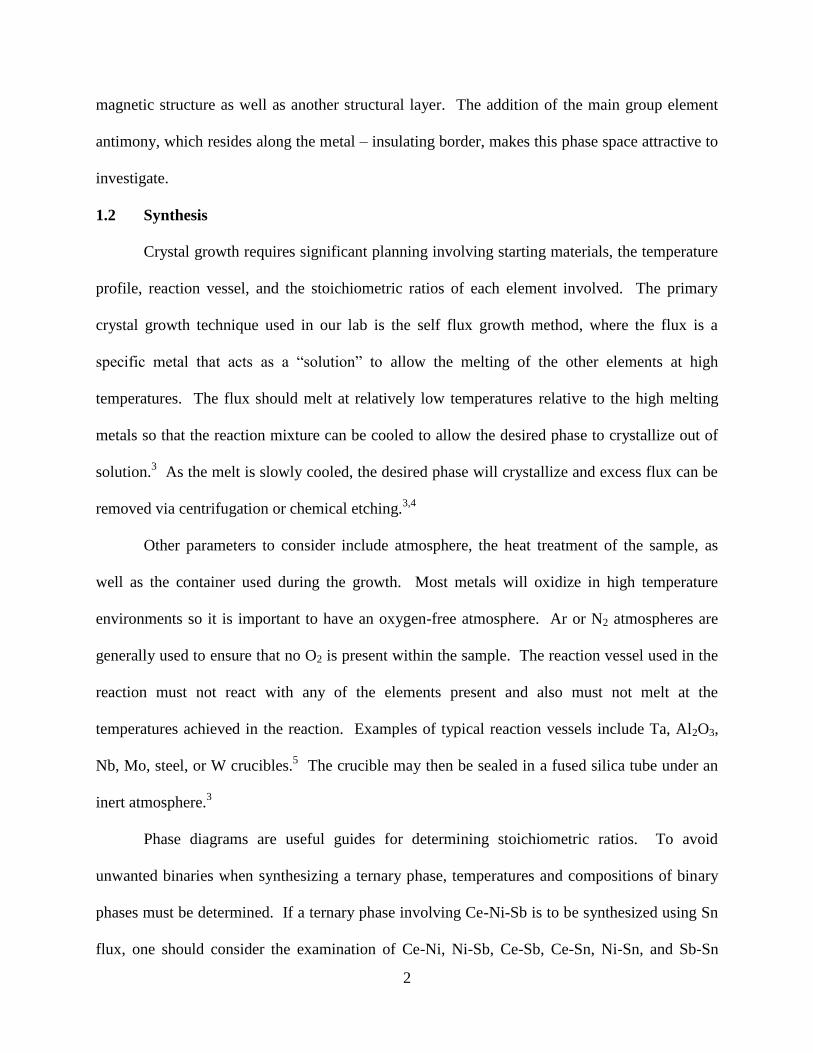
1.2 Synthesis
Crystal growth requires significant planning involving starting materials, the temperature
profile, reaction vessel, and the stoichiometric ratios of each element involved. The primary
crystal growth technique used in our lab is the self flux growth method, where the flux is a
specific metal that acts as a “solution” to allow the melting of the other elements at high
temperatures. The flux should melt at relatively low temperatures relative to the high melting
metals so that the reaction mixture can be cooled to allow the desired phase to crystallize out of
solution.3 As the melt is slowly cooled, the desired phase will crystallize and excess flux can be
removed via centrifugation or chemical etching.3,4
Other parameters to consider include atmosphere, the heat treatment of the sample, as
well as the container used during the growth. Most metals will oxidize in high temperature
environments so it is important to have an oxygen-free atmosphere. Ar or N2 atmospheres are
generally used to ensure that no O2 is present within the sample. The reaction vessel used in the
reaction must not react with any of the elements present and also must not melt at the
temperatures achieved in the reaction. Examples of typical reaction vessels include Ta, Al2O3,
Nb, Mo, steel, or W crucibles.5 The crucible may then be sealed in a fused silica tube under an
inert atmosphere.3
Phase diagrams are useful guides for determining stoichiometric ratios. To avoid
unwanted binaries when synthesizing a ternary phase, temperatures and compositions of binary
phases must be determined. If a ternary phase involving Ce-Ni-Sb is to be synthesized using Sn
flux, one should consider the examination of Ce-Ni, Ni-Sb, Ce-Sb, Ce-Sn, Ni-Sn, and Sb-Sn

3
phase diagrams. Figure 1.1 shows the Ni-Sn binary temperature-composition phase diagram.6
To avoid the synthesis of Ni3Sn4, the molar ratio of Sn should be high enough for the reaction to
be in the liquidus state. We note that Sn melts at 232 °C, and hence to only isolate the desired
phase without Sn encapsulation, one would either remove the reaction from the furnace above
the melting point of Sn or etch the Sn from the surface of the samples.
An alternative to the flux growth method commonly used in our laboratory is an arc-
melting technique. Arc-melting is essentially a “brute-force” welding technique. This technique
is sometimes used when multiple flux-growth experiments have not yielded the desired results.
It is also an easy way to bypass the thermodynamic effects that allow undesired phases to form in
your reaction mixture. Constituent elements are weighed out on stoichiometry to the desired
phase. The elements are then placed together in an electric arc which rapidly melts and binds the
Weight Percent Tin
Atomic Percent Tin
Te
mp
era
ture
C
(Sn)
SnNi
L
0
0
10 20 30 40 50 60 80 9070 100
150
300
450
600
750
1050
1350
900
1200
1500
10 20 30 40 50 60 70 80 90 100
1130 C1160 C
620.5 C
850 C
794.5 C
231.5 CNi3Sn
Ni 3
Sn
2 Ni3Sn4
(Ni)
Figure 1.1 Ni-Sn Phase Diagram adapted from Nash’s Ni-Sn Binary Alloy
Phase Diagram

4
elements together into a button. Then, the arc-melted button is annealed at high temperatures
under vacuum in our furnaces. Occasionally, single crystals are obtained directly from the
annealing process. However, most samples obtained from this method are polycrystalline in
nature. Typically, the polycrystalline sample is then placed in an alumina crucible and a flux is
then added and the reaction vessel undergoes the flux-growth method described above.
Another synthetic technique is used to synthesize polycrystalline oxide samples. Samples
are prepared using a combination of grinding and mixing the constituent oxide powders. The
amounts of oxide powder used are based on the stoichiometry of a solid – state reaction yielding
the desired product. The resulting mixture is then pressed into a small pellet. The pellet is then
heat treated at high temperatures for a predetermined period of time. The resulting pellet is then
ground and remixed again followed by a higher temperature heat treatment. Between each heat
treatment, a powder XRD pattern is taken to identify the phase. This process is continued until
the solid solution is reached with no unreacted oxides remaining. The unreacted oxides show up
as extra peaks in the XRD powder pattern. This technique typically yields only polycrystalline
samples.
1.3 Characterization
1.3.1 Single Crystal X-Ray Diffraction
Single crystal X-ray diffraction is an indispensable technique for determining the crystal
structure of highly crystalline compounds. A beam of X-rays are collinated at the sample and
after impact, the X-rays are scattered in various directions by the electrons and atoms in the
lattice.7 When Bragg’s law (λ = 2dsinθ, where λ is the wavelength of the X-rays, d is the
distance between adjacent planes, and θ is the Bragg angle) is satisfied, diffraction occurs.8 The
scattered X-rays are then recorded by a detector. X-rays are a form of electromagnetic radiation
and possess both amplitude and a phase. The current detectors can record only the amplitude, so

5
only half of the diffraction information needed to calculate electron density is recorded. This is a
well known problem known as the “Phase Problem”. Different techniques have been developed
to overcome the phase problem, and direct methods is the technique used in our group to solve
our structures. Space group, lattice parameters, and atomic positions are obtained from
successfully refined structural models. Structural information such as bond distances, bond
angles, site occupancy, and disorder can also be acquired and are invaluable to fully
understanding the structure.
The Enraf Nonius Kappa CCD Diffractometer was used for all single crystal work in this
document. The X-rays are generated by a Mo Kα X-ray tube where λ = 0.71073 Å. A crystal is
mounted onto the tip of a glass fiber of the goniometer with epoxy and/or vacuum grease.
Temperature is regulated with a cooled nitrogen gas stream produced by an Oxford Cryostream
Cooler. The unit cell parameters were determined from images taken at a rotation of 15 °φ. The
structures were solved using the SIR97 direct methods program.9 The preliminary model of the
structures were then refined using the SHELXL97 program package.10
Refinement of the model
of the structure allows for the correction of many aspects of a crystal structure such as the
addition of extinction coefficients, anisotropic parameters, size, temperature, site occupancy, and
disorder. This part of the process can produce the most correct model for that particular structure
based on the data collected.
Occasionally special sample handling is necessary, particularly if the crystals are air-
sensitive or hygroscopic. In these cases, air exposure must be limited to protect the integrity of
the crystals. The crystals are placed in either mineral oil or paratone-N oil to protect the crystal
surface. Typically, a cooled nitrogen gas stream produced by an Oxford Cryostream Cooler is
used to regulate the temperature of the crystal. For sensitive crystals, the cooled nitrogen gas
stream serves as an additional protective barrier and is used even for room temperature data

6
collections. At low temperatures (typically below 250 K) the epoxy used to secure the crystal to
the tip of the goniometer becomes brittle. For low temperature data collections, the crystal is
simply placed on the tip of the goniometer using either mineral oil or Paratone-N oil. Both of
these oils harden at low temperatures and do not allow the crystal to move while on the tip of the
goniometer. Low temperature data collections are typically used to search for phase transitions.
However, low temperature data is sometimes better than room temperature because the thermal
vibrations of atoms within the crystal are reduced at lower temperatures.
1.3.2 Powder X-Ray Diffraction
Each crystalline sample has a unique powder diffraction pattern. X-ray powder data are
displayed as a pattern with intensity as a function of 2θ. The angles are dependent on the lattice
parameters, lattice type, and wavelength of radiation. The intensity of each peak is dependent on
the scattering of the elements present as well as the amount of sample. Most samples are
compared to the powder patterns in the database from the Joint Committee on Powder
Diffraction Standards (JCPDS) to check for known phases. An unknown sample can be
identified by comparing the pattern to a calculated pattern from a refined model of the new
structure.
X-ray powder diffraction data were collected on a Bruker D8 Advance Powder
Diffractometer with monochromatic Cu K radiation ( = 1.540562 Å) at room temperature.
Data analysis was accomplished using DIFFRACplus
Evaluation Program.11
The ground,
polycrystalline sample is placed onto a no-background holder. It is essential that the powder
sample be flat to avoid errors associated with sample displacement. Figure 1.2 shows the setup
of a powder diffractometer as well as the no-background sample holder used to collect data.

7
1.3.3 Neutron Powder Diffraction
Neutron powder diffraction is a complementary technique used when X-ray diffraction
cannot provide sufficient information. The scattering power of neutrons is advantageous because
the atomic nuclei rather than the electrons are responsible for scattering the radiation. It is
extremely useful in locating light atoms and is able to distinguish between atoms that have
similar scattering. Magnetic structure analysis is also possible with neutron powder diffraction
because the magnetic dipole moment of neutrons may interact with unpaired electrons in the
structure. Neutron powder diffraction (NPD) data were collected at National Institute of
Standards and Technology (NIST) Center for Neutron Research on the powder diffractometer
BT-1. A Cu(311) monochromator with a wavelength (λ) of 1.5403 Å was used.
1.3.4 Elemental Analysis
Because X-ray diffraction cannot distinguish between elements with similar Z, alternative
characterization techniques must be used. The first elemental analysis method used is
inductively coupled plasma-optical emission spectroscopy (ICP-OES) on a Perkin Elmer Optima
Model 5300V. The plasma excites each of the atoms present and upon relaxation light is emitted
and with a polychromatic detector, the amount of each element present can be determined. The
second elemental analysis method employed is energy dispersive spectroscopy. A Hitachi S-
3600N extra-large chamber variable pressure Scanning Electron Microscope (VP-SEM) with an
Sample Window
Metal Sample Holder
X-ray Tube
Focusing Circle
Sample Holder
Detector
Figure 1.2 Illustration of powder diffractometer geometry and sample
holder

8
integrated energy dispersive (EDS) feature was used to collect data. The electrons at ground
state are excited by the beam and an electron from the inner shell is ejected. Then a higher-
energy electron fills the hole left by the inner shell electron and an X-ray is emitted which has
characteristics specific to the element from which it was emitted. This technique is capable of
giving quantitative elemental information and is an excellent complementary technique to X-ray
crystallography.
1.4 Property Measurements
1.4.1 Magnetic Property Measurements
Magnetic susceptibility data (M vs T) were measured by a Quantum Design Physical
Property Measurement System, where M is the magnetization and T is the temperature. Inverse
susceptibility data above the ordering temperature are fitted to Curie-Weiss law to obtain the
magnetic moment and the Weiss temperature, The Curie Weiss law is
T
C
H
M
,
where χ is the magnetic susceptibility, C is the Curie constant, T is the temperature, and θ is the
Weiss constant. Occasionally, a modified version of this law is used when the inverse
susceptibility deviates from Curie-Weiss behavior and an additional constant, χ0, is subtracted
from the magnetic susceptibility. The modified Curie-Weiss equation is
T
C
H
M0 ,
where χ0 is the temperature-independent contribution to the susceptibility. For most of the
magnetic materials in this document χ0 is negligible.
The magnetization as a function of field (M vs H) was also measured by a Quantum
Design Physical Property Measurement System, where M is the magnetization and H is the
applied magnetic field. The saturation moment from this data is compared to a calculated value.
The calculated saturation moment, µsat = -gµBJ, where g is given by the Landé equation, µB is a
bohr magneton, and J is the sum of the orbital and spin angular momenta.12
The Landé equation

9
is defined as )1(2
)1()1()1(1
JJ
LLSSJJg for a free atom. Typically, the magnetization
curve for a ferromagnet displays hysteresis.
Transport Property Measurements
Resistivity as a function of temperature is typically measured on a single crystal and is
defined as the resistance generated by collisions of electrons with phonons or impurities in the
crystal lattice.12
Electrical resistivity is defined as L
AR , where R is the resistance, A is the
area of the crystal, and L is the length of the crystal. A sudden drop in the resistivity to zero
indicates a superconducting transition. Identifying and understanding materials with these
superconducting transitions may lead to the design of materials with superconducting behavior at
room temperature. Magnetoresistance is defined as %1000
0
and is plotted as a function
of changing field.12
The magnetoresistance of a typical metal is on the order of ~10 %.
Materials that possess larger magnetoresistance behavior at room temperature have potential
applications as various spintronic materials. Understanding both of these transport property
behaviors are important in understanding and designing new materials.
1.5 Systems Investigated in This Document
The systems that are discussed in this dissertation focus on the structural studies of
selected antimonides and double molybdates. Chapter 2 will focus on the synthesis, structure
determination, and physical properties of LnNi(Sb,Sn)3 (Ln = La-Nd, Sm, Gd, Tb). The
relationship of this structure type to other similar antimonide structure types will be explored.
Chapter 3 will discuss the ramifications of substituting Co for Ni in both the structure and
physical properties of CeNixCo1-xSb3. Chapter 4 involves the systematic substitution of Ni for
Cu in Ce(Cu1-xNix)ySb2 and focuses on the effects on the magnetoresistance behavior. Structural

10
effects and magnetic properties are also explored. Chapter 5 presents a structural study of the
effects of transition metal substitution of double molybates Rb4M(MoO4)3 (M = Mn, Zn, and
Cu). The Zn and Cu analogues both adopt new structure types. Temperature dependent phase
transitions are explored for all analogues. Chapter 6 provides brief conclusions and general
overview of the dissertation. The appendices include structural studies of various side projects.
Appendix 1 focuses on the structural determination of LnPdSb3, which is a new structure type.
Appendix 2 discusses the structure and physical properties of EuCu9Sn4. Appendix 3 presents
the structural confirmation of VB2. Accurate lattice parameters were necessary for energy band
calculations. Appendix 4 provides structural data from neutron powder diffraction and magnetic
properties of Y2-xCexTi2O7. Appendix 5 contains unpublished crystallographic information files
for the molybdates discussed in Chapter 5. Letters of permission to reuse published work are
provided in Appendix 6.
1.6 References
(1) Canfield, P. C. Nature 2008, 4, 167-169.
(2) Papoian, G. A.; Hoffmann, R. Angew. Chem. Int. Ed. 2000, 39, 2409-2448.
(3) Canfield, P. C.; Fisk, Z. Philos. Mag. B 1992, 65, 1117-23.
(4) Kanatzidis, M. G.; Pöttgen, R.; Jeitschko, W. Angew. Chem. Int. Ed. 2005, 44, 6996-
7023.
(5) Fisk, Z.; Remeika, J. P. Handbook on the Physics and Chemistry of Rare Earths;
Elsevier: Amsterdam, 1989; Vol. 12.
(6) Nash, P.; Nash, A. Bull. Alloy Phase Diagrams 1985, 6, 350-359.
(7) Cullity, B. D. Elements of X-Ray Diffraction; 2nd ed.; Addison-Wesley Publishing
Company, Inc: Reading, Massachusetts, 1978.
(8) Clegg, W.; Blake, A. J.; Gould, R. O.; Main, P. Crystal Structure Analysis Principles and
Practice; Oxford University Press: Oxford, NY, 2001.

11
(9) Altomare, A.; Burla, M. C.; Camalli, M.; Cascarno, G. L.; Giacovazzo, A.; Guagliardi,
A.; Moliterni, A. G. G.; Polidori, G.; Spagna, R. J. J. Appl. Crystallogr. 1999, 32, 115-
119.
(10) Sheldrick, G. M.; University of Gottingen: Germany, 1997.
(11) 6.0 ed.; Bruker, AXS: Karlsruhe, West Germany, 2000.
(12) Kittel, C.; 7th ed.; John Wiley & Sons, Inc.: New York, 1995.
12
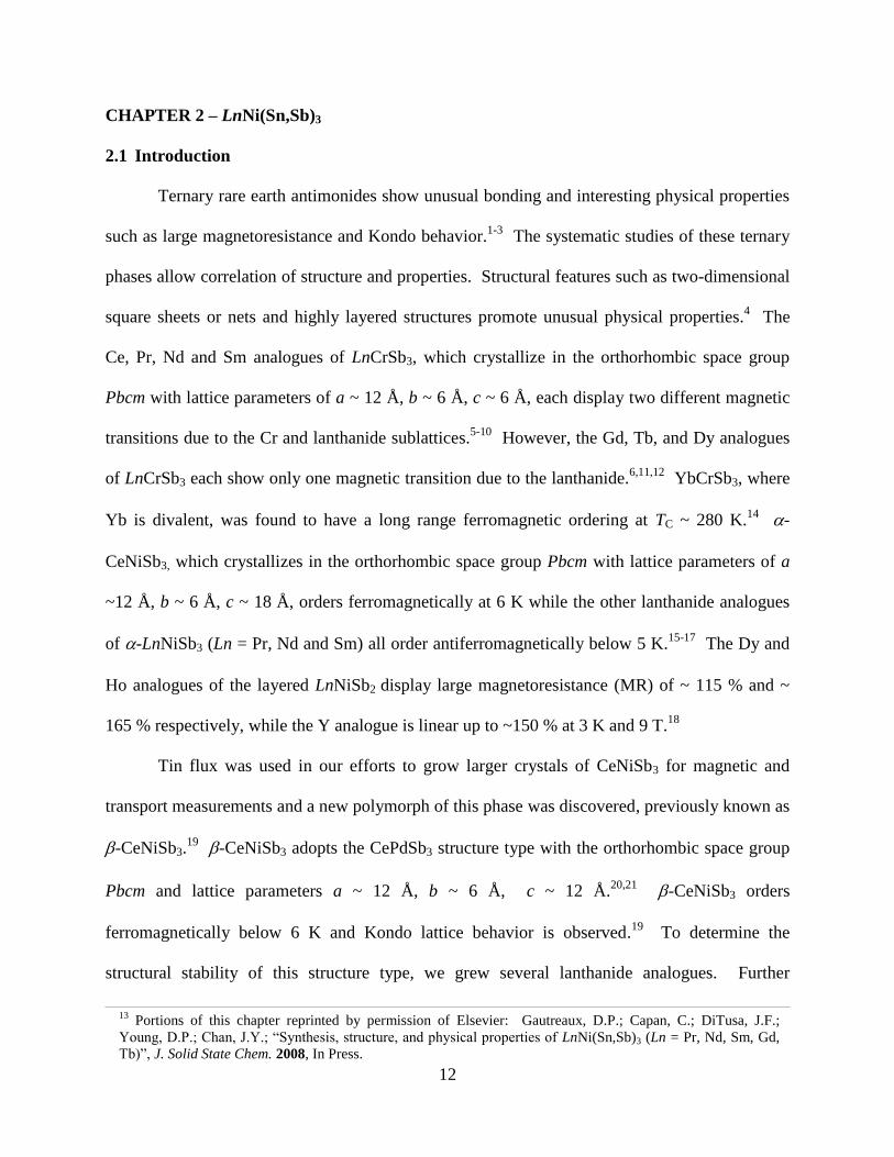
CHAPTER 2 – LnNi(Sn,Sb)3
2.1 Introduction
Ternary rare earth antimonides show unusual bonding and interesting physical properties
such as large magnetoresistance and Kondo behavior.1-3
The systematic studies of these ternary
phases allow correlation of structure and properties. Structural features such as two-dimensional
square sheets or nets and highly layered structures promote unusual physical properties.4 The
Ce, Pr, Nd and Sm analogues of LnCrSb3, which crystallize in the orthorhombic space group
Pbcm with lattice parameters of a ~ 12 Å, b ~ 6 Å, c ~ 6 Å, each display two different magnetic
transitions due to the Cr and lanthanide sublattices.5-10
However, the Gd, Tb, and Dy analogues
of LnCrSb3 each show only one magnetic transition due to the lanthanide.6,11,12
YbCrSb3, where
Yb is divalent, was found to have a long range ferromagnetic ordering at TC ~ 280 K.14
-
CeNiSb3, which crystallizes in the orthorhombic space group Pbcm with lattice parameters of a
~12 Å, b ~ 6 Å, c ~ 18 Å, orders ferromagnetically at 6 K while the other lanthanide analogues
of -LnNiSb3 (Ln = Pr, Nd and Sm) all order antiferromagnetically below 5 K.15-17
The Dy and
Ho analogues of the layered LnNiSb2 display large magnetoresistance (MR) of ~ 115 % and ~
165 % respectively, while the Y analogue is linear up to ~150 % at 3 K and 9 T.18
Tin flux was used in our efforts to grow larger crystals of CeNiSb3 for magnetic and
transport measurements and a new polymorph of this phase was discovered, previously known as
-CeNiSb3.19
-CeNiSb3 adopts the CePdSb3 structure type with the orthorhombic space group
Pbcm and lattice parameters a ~ 12 Å, b ~ 6 Å, c ~ 12 Å.20,21
-CeNiSb3 orders
ferromagnetically below 6 K and Kondo lattice behavior is observed.19
To determine the
structural stability of this structure type, we grew several lanthanide analogues. Further
13 Portions of this chapter reprinted by permission of Elsevier: Gautreaux, D.P.; Capan, C.; DiTusa, J.F.;
Young, D.P.; Chan, J.Y.; “Synthesis, structure, and physical properties of LnNi(Sn,Sb)3 (Ln = Pr, Nd, Sm, Gd,
Tb)”, J. Solid State Chem. 2008, In Press.
13
investigation of this structure led to the discovery that Sn was incorporated into the crystal
structure. The crystal growth, structure, magnetic properties of LnNi(Sn,Sb)3 (Ln = La, Ce, Pr,
Nd, Sm, Gd, and Tb) are reported herein.
2.2 Experimental
2.2.1 Synthesis
Single crystals of LnNi(Sn,Sb)3 (Ln = La, Ce, Pr, Nd, Sm, Gd, or Tb) were prepared
using excess Sn as the flux. La, Ce, Pr, Nd, Sm, Gd, or Tb pieces (99.9%, Alfa Aesar), Ni
powder (99.999%, Alfa Aesar), Sb shot (99.999%, Alfa Aesar), and Sn shot (99.8%, Alfa Aesar)
were placed in an alumina crucible in a 1:2:3:15 molar ratio. The crucible was sealed into an
evacuated fused-silica tube. The reaction vessel was heated to 1150 °C where the temperature
was held constant for 24 h and then cooled 5 °C h-1
to 300 °C. After dwelling at 300 °C, the
excess Sn flux was removed by centrifugation. The reaction mixtures contained silver plate-like
crystals with dimensions up to 0.08 x 3 x 5 mm3 for all analogues except Tb which contained
plate-like crystals with dimensions up to 0.08 x 0.5 x 0.5 mm3. Most samples also contained
silver rod shaped crystals with dimensions of 1 x 1 x 5 mm3. The plates were determined to be
the desired product, while the predominant phase is the rod-shaped binary, Ni3Sn4. When
exposed to air and moisture, there is no visible surface degradation to both compounds over a
period of months.
Flux growth syntheses with other molar ratios such as 1:1:3:20 and 1:1:3:15 for the latter
rare earth analogues with Sn flux were investigated; however, yield was less than 10%. The
addition of excess Ni (1:2:3:15) resulted in an increased yield of LnNi(Sn,Sb)3. We note that
smaller lanthanide metals, Dy and Yb, yielded binary phases. Adjusting the spin temperature
from 300 °C to 670 °C or 450 °C, also yielded different results. At 670 °C, CeNi(Sn,Sb)3 and
CeSb were obtained while at 450 °C CeNi(Sn,Sb)3, CeSb, and Ni3Sn4 were obtained. However,

14
the yield of the desired CeNi(Sn,Sb)3 was lower at both 670 °C and 450 °C than at 300 °C. Arc-
melting the constituent elements Ce, Ni, and Sb (1:1:3) without Sn yields the α-CeNiSb3
structure type, therefore α-CeNiSb3 must be a line compound. Arc-melting Ce:Ni:Sb with 5 or
10% Sn followed by annealing at 1150 °C for 3 days in an evacuated fused-silica tube, allows for
the substitution of Sn within the α-CeNiSb3 structure. This is determined by an increase of the
lattice parameters obtained from single-crystal X-ray diffraction. Single crystals of α-CeNiSb3
can be “transformed” into CeNi(Sn,Sb)3.19
Unground single crystals of α-CeNiSb3 were placed
into an alumina crucible with a 20 fold excess of Sn flux. After placing the crucible into an
evacuated fused-silica tube, the reaction vessel underwent the heat treatment described above
and was removed from the furnace at 300 °C. Approximately half of the crystals were
“transformed” into CeNi(Sn,Sb)3 while the other half maintained the α-CeNiSb3 structure type.
These results were confirmed by single crystal X-ray diffraction.
2.2.2 Single Crystal X-ray Diffraction
A typical crystal with dimensions of ~ 0.08 x 0.08 x 0.1 mm3 was mounted onto a glass
fiber of a goniometer with epoxy and placed on a Nonius Kappa CCD X-ray diffractometer
(MoKα = 0.71073 Å). Data collection parameters and crystallographic data are listed in Table
2.1 for LnNi(Sn,Sb)3 (Ln = Pr, Sm, Gd, Tb). The unit cell parameters were determined from
images taken at a rotation of 15 °φ. The model of the structure was refined by direct methods
using SHELXL97.22
The data were corrected for absorption and the displacement parameters
were refined as anisotropic. Atomic coordinates and anisotropic displacement parameters are
provided in Table 2.2. The R-factors for all compounds are reasonable with the exception of the
Nd analogue. After multiple data collections, it was determined that this analogues has lower
crystal quality based on higher chi2 values.

15
Table 2.1 Crystallographic Data for LnNi(Sn,Sb)3 (Ln = Pr, Sm, Gd, or Tb)
La Ce Pr Nd Sm Gd Tb
Space Group Pbcm Pbcm Pbcm Pbcm Pbcm Pbcm Pbcm
a (Å) 13.0970(2) 12.9170(2) 12.843(3) 12.771(2) 12.651(1) 12.565(2) 12.450(1)
b (Å) 6.1400(4) 6.1210(5) 6.105(7) 6.093(4) 6.083(2) 6.072(3) 6.060(2)
c (Å) 12.1270(4) 12.0930(6) 12.056(6) 12.021(4) 11.994(2) 11.973(4) 11.935(2)
V (Å3) 975.20(4) 956.13(9) 945.3(12) 935.4(7) 923.0(3) 913.5(6) 900.5(3)
Size (mm3) 0.02/0.05/0.05 0.08/0.08/0.1 0.01/0.04/0.05 0.08/0.08/0.01 0.01/0.03/0.05 0.02/0.05/0.05 0.01/0.03/0.06
Z 8 8 8 8 8 8 8
Temp (°C) 25(2) 25(2) 24(2) 25(2) 25(2) 25(2) 25(2)
Density(g cm-1) 7.668 7.837 7.938 8.069 8.266 8.452 8.599
Range (°) 1.55-30.03 3.15-29.99 3.17-30.08 3.19-29.97 3.22-30.04 3.25-29.98 3.27-30.01
μ (mm-1
) 28.573 29.728 30.747 31.755 33.655 35.670 37.163
Rint 0.0396 0.0181 0.0610 0.0626 0.0629 0.0557 0.0478
Collected Ref. 2677 2601 2541 2384 2492 2434 2469
Unique Ref. 1491 1445 1439 1400 1400 1377 1380
h -17 h 17 -17 h 17 -17 h 17 -17 h 17 -17 h 17 -17 h 17 -17 h 17
k -8 k 8 -8 k 8 -8 k 8 -8 k 8 -8 k 8 -8 k 8 -8 k 8
l - 16 l 16 - 16 l 16 - 16 l 16 - 16 l 16 -16 l 16 -16 l 16 -16 l 16
max (e Å-3
) 7.531 5.514 4.551 9.921 6.822 8.931 7.860
min (e Å-3
) -5.625 -1.705 -3.704 -10.886 -12.674 -8.063 -12.168
Extinction 0.0056(5) 0.00030(7) 0.00050(10) 0.0014(3) 0.0064(5) 0.00057(19) 0.0064(5) a
)](2[ 22 FFR 0.0627 0.0282 0.0522 0.0970 0.0745 0.0855 0.0618 b )( 2
2 FwR 0.1779 0.0716 0.1314 0.2639 0.1832 0.2092 0.1621
a 001 /)( FFFFR c
b 2/122
0
22
0
2
0 ])([/)]([)( FwFFwFR cw ; 2 2 2
01/ [ ( ) (0.1403 ) 1.2003 ]w F P P ,
2 2 2
01/ [ ( ) (0.0140 ) 12.8728 ]w F P P 2 2 2
01/ [ ( ) (0.0697 ) 8.8849 ]w F P P , 2 2 2
01/ [ ( ) (0.1728 ) ]w F P ,
]3454.2)1232.0()(/[1 22
0
2 PPFw , ])1586.0()(/[1 22
0
2 PFw , ]3692.9)1078.0()(/[1 22
0
2 PPFw
for La, Ce, Pr, Nd, Sm, Gd, and Tb respectively
2.2.3 Elemental Analysis
Elemental analysis using EDX was performed using a Hitachi S-3600N variable pressure
scanning electron microscope (VP-SEM) and a stoichiometry of LnNiSnSb2 was obtained.
Elemental analysis of the Sn:Sb composition of the crystals was performed using Optical
Emission Spectroscopy (ICP-OES) on a Perkin Elmer Optima Model 5300V for all analogues
(Pr, Nd, Sm, Gd, Tb). The Sn:Sb compositions obtained for each analogue are as follows: Pr –
Sn0.97Sb2.03, Nd – Sn0.92Sb2.08, Sm – Sn1.24Sb1.76, Gd – Sn0.99Sb2.01, Tb – Sn0.59Sb2.41. This

16
confirms the presence of Sn in the structure and is consistent with the EDX results previously
mentioned.
Table 2.2 Atomic Positions and Displacement Parameters for LnNi(Sn,Sb)3
(Ln = La, Ce, Pr, Sm, Gd, or Tb; X = Sn/Sb)
Atom Wyckoff site x y z Ueq (Å2)
a
La1 4c 0.69985(7) ¼ 0 0.0077(3)
La2 4d 0.30410(7) 0.26099(11) ¾ 0.0077(3)
Ni1 8e 0.10248(10) 0.0302(2) 0.86359(9) 0.0105(4)
X1 4c 0.97547(8) ¼ 0 0.0128(3)
X2 4d 0.78994(8) 0.25128(12) ¾ 0.0080(3)
X3 8e 0.50131(5) 0.50751(9) 0.87603(4) 0.0087(3)
X4 4c 0.21497(8) ¼ 0 0.0079(3)
X5 4d 0.94673(7) 0.88313(14) ¾ 0.0121(3)
Ce1 4c 0.69921(4) ¼ 0 0.0070(1)
Ce2 4d 0.30482(4) 0.26209(7) ¾ 0.0068(1)
Ni1 8e 0.10429(6) 0.0302(1) 0.86352(6) 0.0094(2)
X1 4c 0.97482(5) ¼ 0 0.0112(2)
X2 4d 0.78593(5) 0.25134(8) ¾ 0.0075(2)
X3 8e 0.50154(3) 0.50804(6) 0.8759(3) 0.0081(1)
X4 4c 0.21859(5) ¼ 0 0.0074(2)
X5 4d 0.94614(4) 0.8837(1) ¾ 0.0109(2)
Pr1 4c 0.69919(7) ¼ 0 0.0123(3)
Pr2 4d 0.30501(7) 0.26236(17) ¾ 0.0120(3)
Ni1 8e 0.10491(13) 0.0301(3) 0.86371(14) 0.0146(4)
X1 4c 0.97501(10) ¼ 0 0.0164(3)
X2 4d 0.78459(9) 0.2512(2) ¾ 0.0131(3)
X3 8e 0.50157(6) 0.50801(14) 0.87592(6) 0.0130(3)
X4 4c 0.22006(9) ¼ 0 0.0126(3)
X5 4d 0.94559(9) 0.8841(2) ¾ 0.0167(3)
Nd1 4c 0.69855(10) ¼ 0 0.0057(4)
Nd2 4d 0.30558(9) 0.26297(17) ¾ 0.0058(4)
Ni1 8e 0.10590(13) 0.0304(3) 0.86355(15) 0.0075(5)
X1 4c 0.97456(11) ¼ 0 0.0082(5)
X2 4d 0.78284(12) 0.25064(19) ¾ 0.0058(5)
X3 8e 0.50177(6) 0.50821(15) 0.87595(7) 0.0068(5)
X4 4c 0.22184(12) ¼ 0 0.0058(5)
X5 4d 0.94564(9) 0.8848(2) ¾ 0.0087(5)
Sm1 4c 0.69875(6) ¼ 0 0.0078(3)
Sm2 4d 0.30574(6) 0.26435(13) ¾ 0.0078(3)
Ni1 8e 0.10733(10) 0.0297(2) 0.86354(11) 0.0092(4)
X1 4c 0.97476(8) ¼ 0 0.0107(3)
X2 4d 0.77989(9) 0.25034(14) ¾ 0.0081(3)
X3 8e 0.50213(4) 0.50858(11) 0.87599(6) 0.0090(3)
X4 4c 0.22485(9) ¼ 0 0.0079(3)
X5 4d 0.94515(7) 0.88488(16) ¾ 0.0106(3)
Gd1 4c 0.69800(8) ¼ 0 0.0077(4)
Gd2 4d 0.30634(8) 0.26474(17) ¾ 0.0077(4)
Ni1 8e 0.10870(16) 0.0295(3) 0.86342(14) 0.0103(5)
X1 4c 0.97487(11) ¼ 0 0.0115(4)
X2 4d 0.77844(12) 0.2497(2) ¾ 0.0086(4)
17
Table 2.2 (cont.) Atom Wyckoff site x y z Ueq (Å
2)
a
X3 8e 0.50226(7) 0.50904(15) 0.87588(7) 0.0099(4)
X4 4c 0.22648(12) ¼ 0 0.0081(4)
X5 4d 0.94488(11) 0.8846(2) ¾ 0.0116(4)
Tb1 4c 0.69785(7) ¼ 0 0.0068(3)
Tb2 4d 0.30665(7) 0.26545(13) ¾ 0.0064(3)
Ni1 8e 0.11013(12) 0.0288(3) 0.86377(12) 0.0085(4)
X1 4c 0.97497(9) ¼ 0 0.0097(3)
X2 4d 0.77590(10) 0.24843(16) ¾ 0.0073(3)
X3 8e 0.50259(5) 0.50885(12) 0.87582(6) 0.0075(3)
X4 4c 0.22913(10) ¼ 0 0.0070(3)
X5 4d 0.94480(8) 0.88451(18) ¾ 0.0106(3) aUeq is defined as one-third of the trace of the orthogonalized Uij tensor.
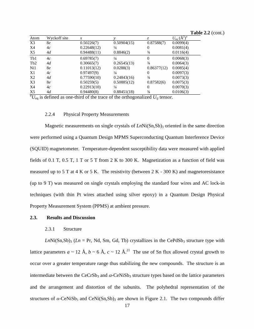
2.2.4 Physical Property Measurements
Magnetic measurements on single crystals of LnNi(Sn,Sb)3 oriented in the same direction
were performed using a Quantum Design MPMS Superconducting Quantum Interference Device
(SQUID) magnetometer. Temperature-dependent susceptibility data were measured with applied
fields of 0.1 T, 0.5 T, 1 T or 5 T from 2 K to 300 K. Magnetization as a function of field was
measured up to 5 T at 4 K or 5 K. The resistivity (between 2 K - 300 K) and magnetoresistance
(up to 9 T) was measured on single crystals employing the standard four wires and AC lock-in
techniques (with thin Pt wires attached using silver epoxy) in a Quantum Design Physical
Property Measurement System (PPMS) at ambient pressure.
2.3. Results and Discussion
2.3.1 Structure
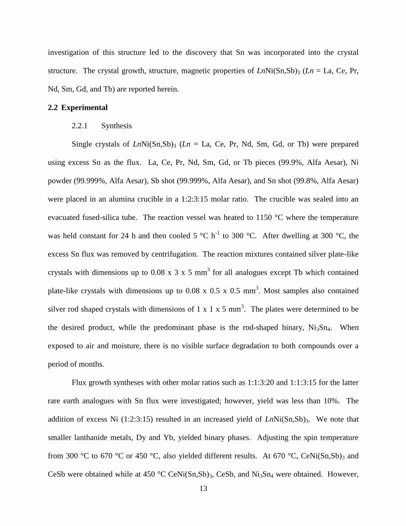
LnNi(Sn,Sb)3 (Ln = Pr, Nd, Sm, Gd, Tb) crystallizes in the CePdSb3 structure type with
lattice parameters a ~ 12 Å, b ~ 6 Å, c ~ 12 Å.21
The use of Sn flux allowed crystal growth to
occur over a greater temperature range thus stabilizing the new compounds. The structure is an
intermediate between the CeCrSb3 and -CeNiSb3 structure types based on the lattice parameters
and the arrangement and distortion of the subunits. The polyhedral representation of the
structures of α-CeNiSb3 and CeNi(Sn,Sb)3 are shown in Figure 2.1. The two compounds differ
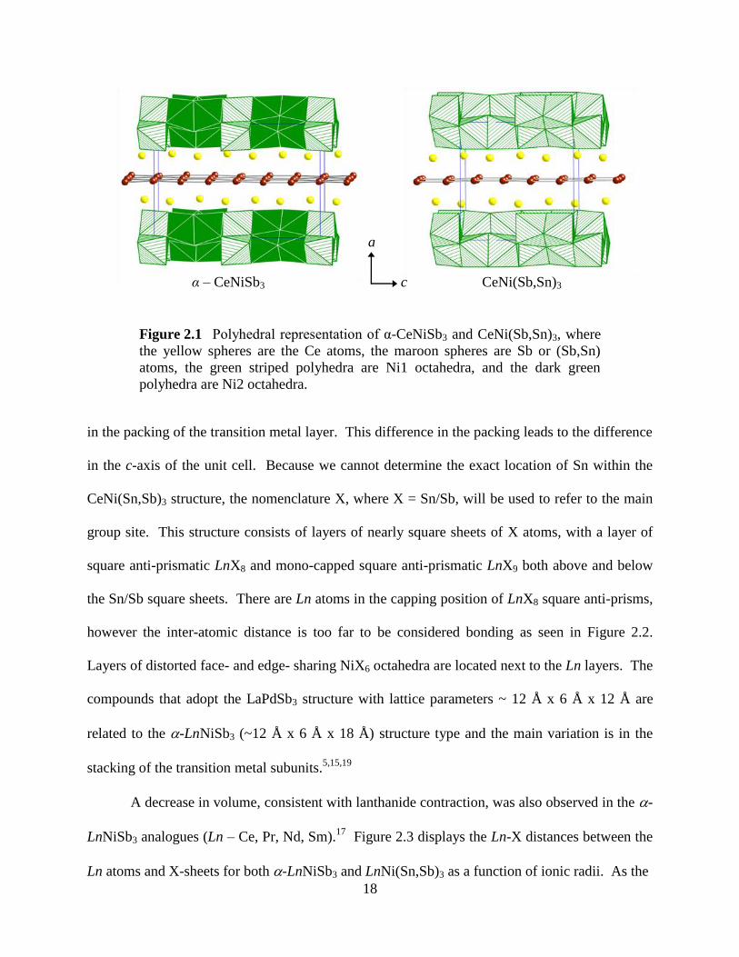
18
in the packing of the transition metal layer. This difference in the packing leads to the difference
in the c-axis of the unit cell. Because we cannot determine the exact location of Sn within the
CeNi(Sn,Sb)3 structure, the nomenclature X, where X = Sn/Sb, will be used to refer to the main
group site. This structure consists of layers of nearly square sheets of X atoms, with a layer of
square anti-prismatic LnX8 and mono-capped square anti-prismatic LnX9 both above and below
the Sn/Sb square sheets. There are Ln atoms in the capping position of LnX8 square anti-prisms,
however the inter-atomic distance is too far to be considered bonding as seen in Figure 2.2.
Layers of distorted face- and edge- sharing NiX6 octahedra are located next to the Ln layers. The
compounds that adopt the LaPdSb3 structure with lattice parameters ~ 12 Å x 6 Å x 12 Å are
related to the -LnNiSb3 (~12 Å x 6 Å x 18 Å) structure type and the main variation is in the
stacking of the transition metal subunits.5,15,19
A decrease in volume, consistent with lanthanide contraction, was also observed in the -
LnNiSb3 analogues (Ln – Ce, Pr, Nd, Sm).17
Figure 2.3 displays the Ln-X distances between the
Ln atoms and X-sheets for both -LnNiSb3 and LnNi(Sn,Sb)3 as a function of ionic radii. As the
a
c α – CeNiSb3 CeNi(Sb,Sn)3
Figure 2.1 Polyhedral representation of α-CeNiSb3 and CeNi(Sb,Sn)3, where
the yellow spheres are the Ce atoms, the maroon spheres are Sb or (Sb,Sn)
atoms, the green striped polyhedra are Ni1 octahedra, and the dark green
polyhedra are Ni2 octahedra.

19
lanthanide radii decreases, the distance between the Ln atoms and Sb or Sn/Sb nets decreases.
Selected interatomic distances of LnNi(Sn,Sb)3 (Ln = La-Nd, Sm, Gd, or Tb) are shown in Table
2.3. As expected, the Ln-X distances along the a-axis decrease as a function of smaller
lanthanide. In LnNi(Sn,Sb)3, the Sn/Sb net layer is formed by four-bonded X3 atoms while in
the -phase, the Sb square net is formed by four Sb1 and Sb3 atoms and is highly distorted.15
As
smaller lanthanides are substituted into the structure, the X - X distances within the sheets
decrease slightly, and the angles are slightly more distorted. Under our growth conditions, the
LnNi(Sn,Sb)3 phase can be adopted for Ce, Pr, Nd, Sm, Gd, and Tb while only Ce, Pr, Nd, and
Sm analogues can be adopted for the -LnNiSb3 structure type. This may be due to the decrease
in lanthanide to Sb net distances, leading to a strain on the structure type. It is also important to
note that for smaller rare earth elements, Gd – Er, and Y, the tetragonal LnNiSb2 structure type is
adopted under our growth conditions. The Gd and Tb analogues of LnNi(Sn,Sb)3 the
experimental yield was extremely small and the crystal size was almost microscopic. This is
Figure 2.2 Environment of Ln sites of LnNi(Sn,Sb)3 as viewed down the b-
axis. Ln1 adopts a square anti-prismatic environment, while Ln2 adopts a
mono-capped square anti-prism.
Ln1Ln2
Sb5Sb1
Sb3
a
c
Sb3
Sb3
Sb3
Sb3
Sb3
Sb3
Sb4
Sb4Sb4 Sb2
Sb2
Sb2

20
further indication that the structure type is strained and leads to the more stable LnNiSb2
structure type.
Table 2.3 Selected Interatomic Distances (Å) of LnNi(Sn,Sb)3 (Ln = La, Ce, Pr, Sm, Gd, or
Tb; X = Sn/Sb)
La Ce Pr Nd Sm Gd Tb
Ln1-X1 3.6099(13) 3.501(8) 3.5423(17) 3.5249(18) 3.4918(12) 3.4789(17) 3.4501(14)
Ln1-X2 (x2) 3.2533(5) 3.2241(3) 3.2074(15) 3.1923(11) 3.1693(6) 3.1593(11) 3.1380(7)
Ln1-X3 (x2) 3.3791(9) 3.3419(5) 3.3269(15) 3.3074(14) 3.2906(9) 3.2681(13) 3.2496(10)
Ln1-X3 (x2) 3.3942(9) 3.3562(3) 3.3408(15) 3.3188(14) 3.2976(9) 3.2759(13) 3.2506(10)
Ln1-X4 (x2) 3.2672(5) 3.2395(3) 3.224(3) 3.212(2) 3.1914(11) 3.1808(15) 3.1634(11)
Ln2-X2 3.2526(10) 3.2159(7) 3.198(4) 3.179(2) 3.1485(15) 3.131(2) 3.1021(16)
Ln2-X2 3.3633(10) 3.3388(7) 3.326(4) 3.320(2) 3.3091(15) 3.304(2) 3.2974(16)
Ln2-X3 (x2) 3.3545(9) 3.3158(6) 3.2994(16) 3.2795(14) 3.2575(9) 3.2351(13) 3.2115(10)
Ln2-X3 (x2) 3.3613(10) 3.3232(6) 3.3055(15) 3.2867(14) 3.2654(9) 3.2453(13) 3.2221(10)
Ln2-X4 (x2) 3.2503(5) 3.2228(3) 3.2063(15) 3.1908(11) 3.1695(7) 3.1582(11) 3.1374(7)
Ln2-X5 3.3697(12) 3.3261(7) 3.3032(17) 3.2930(17) 3.2576(12) 3.2394(17) 3.2126(13)
X3-X3 3.0083(11) 3.0020(7) 2.994(2) 2.985(2) 2.9772(14) 2.9748(19) 2.9667(15)
X3-X3 3.0568(11) 3.0464(7) 3.036(2) 3.028(2) 3.0221(15) 3.0142(19) 3.0034(15)
X3-X3 3.0702(2) 3.0607(6) 3.053(4) 3.047(2) 3.0420(10) 3.0365(15) 3.0307(10)
Ni-X1 2.25957(13) 2.5901(8) 2.584(2) 2.582(2) 2.5790(15) 2.580(2) 2.5730(17)
Ni-X1 2.7066(14) 2.7456(15) 2.699(2) 2.701(2) 2.6997(15) 2.701(2) 2.6968(17)
Ni-X2 2.6105(14) 2.6093(9) 2.606(2) 2.605(2) 2.6033(16) 2.596(2) 2.5968(18)
Ni-X4 2.5927(13) 2.5913(8) 2.586(2) 2.583(2) 2.5857(15) 2.580(2) 2.5760(17)
Ni-X5 2.6217(15) 2.6193(9) 2.619(2) 2.615(2) 2.6153(15) 2.618(2) 2.6163(18)
Ni-X5 2.6477(14) 2.6444(10) 2.641(3) 2.638(2) 2.6390(17) 2.636(2) 2.638(2)
Ni-Ni 2.755(2) 2.7459(15) 2.742(4) 2.730(4) 2.724(3) 2.716(3) 2.716(3)
3.20
3.22
3.24
3.26
3.28
3.30
3.32
3.34
3.20
3.22
3.24
3.26
3.28
3.30
3.32
3.34
0.960.981.001.021.041.061.08
Ln
1-S
b1
-LnN
iSb
3Ln
1-X
3 L
nN
i(Sn,S
b)3
Ln3+
Ionic Radii
CeSm
Nd
Pr
Ce
Pr
Nd
Sm
Gd
Tb-LnNiSb3
LnNi(Sn,Sb)3
Figure 2.3 Plot of Ln-X (X = Sn,Sb) distances as a function of lanthanide for
both -LnNiSb3 and LnNi(Sn,Sb)3.
21
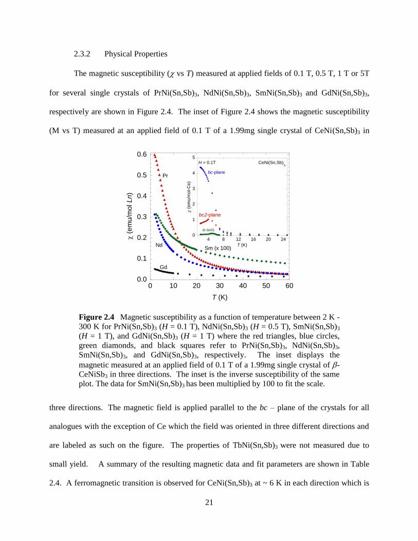
2.3.2 Physical Properties
The magnetic susceptibility ( vs T) measured at applied fields of 0.1 T, 0.5 T, 1 T or 5T
for several single crystals of PrNi(Sn,Sb)3, NdNi(Sn,Sb)3, SmNi(Sn,Sb)3 and GdNi(Sn,Sb)3,
respectively are shown in Figure 2.4. The inset of Figure 2.4 shows the magnetic susceptibility
(M vs T) measured at an applied field of 0.1 T of a 1.99mg single crystal of CeNi(Sn,Sb)3 in
three directions. The magnetic field is applied parallel to the bc – plane of the crystals for all
analogues with the exception of Ce which the field was oriented in three different directions and
are labeled as such on the figure. The properties of TbNi(Sn,Sb)3 were not measured due to
small yield. A summary of the resulting magnetic data and fit parameters are shown in Table
2.4. A ferromagnetic transition is observed for CeNi(Sn,Sb)3 at ~ 6 K in each direction which is
0.0
0.1
0.2
0.3
0.4
0.5
0.6
0 10 20 30 40 50 60
(
em
u/m
ol Ln)
T (K)
Pr
Sm (x 100)Nd
Gd
0
1
2
3
4
5
4 8 12 16 20 24
(
em
u/m
ol-C
e)
T (K)
H = 0.1T
bc-plane
bc2-plane
a-axis
CeNi(Sn,Sb)3
Figure 2.4 Magnetic susceptibility as a function of temperature between 2 K -
300 K for PrNi(Sn,Sb)3 (H = 0.1 T), NdNi(Sn,Sb)3 (H = 0.5 T), SmNi(Sn,Sb)3
(H = 1 T), and GdNi(Sn,Sb)3 (H = 1 T) where the red triangles, blue circles,
green diamonds, and black squares refer to PrNi(Sn,Sb)3, NdNi(Sn,Sb)3,
SmNi(Sn,Sb)3, and GdNi(Sn,Sb)3, respectively. The inset displays the
magnetic measured at an applied field of 0.1 T of a 1.99mg single crystal of -
CeNiSb3 in three directions. The inset is the inverse susceptibility of the same
plot. The data for SmNi(Sn,Sb)3 has been multiplied by 100 to fit the scale.

22
similar to the (T) of the -form.23
From the inverse susceptibility along the a, b and c-axes, the
experimental effective moments of 1.80, 2.45 and 2.38 B and Weiss temperatures () of 22.8,
8.6 and 1.4 K respectively along each axis obeys Curie-Weiss law. The average eff of 2.23 B is
slightly smaller than the calculated 2.54 B for the Ce3+
ion. PrNi(Sn,Sb)3 does not appear to
order down to 2 K. However, the possibility remains that this sample may order below 2 K as
signs of ordering can be seen in the magnetization near 2 K. An effective moment of 3.65 B
and a Weiss temperature () of ~ -1 K were obtained from a modified Curie Weiss fit χ = χ0 +
C/(T+θ) between 100 K – 300 K. The eff of 3.68 B is slightly larger than the calculated
moment of 3.57 B for the Pr3+
ion and is consistent with the magnetic contribution coming
solely from the Pr. NdNi(Sn,Sb)3 is paramagnetic down to 2 K. Fits to the inverse susceptibility
between 2 K – 300 K reveal an effective moment of 3.93 μB and a Weiss temperature, ~ -4 K.
The experimental moment of 3.93 B is slightly larger than the calculated moment of 3.62 B for
the Nd3+
ion. SmNi(Sn,Sb)3 appears be paramagnetic down to 2.5 K. An effective moment of
0.65 μB and a Weiss temperature () of ~ -19 K were obtained with a Curie-Weiss fit from 50 –
300 K. The experimental moment is slightly smaller than the expected moment of 0.84 μB for
Sm3+
. GdNi(Sn,Sb)3 is also paramagnetic down to 2 K and an effective moment of 7.47 µB and a
Weiss temperature (θ) of ~ -403 K were obtained from the modified Curie-Weiss fit. The
expected moment for Gd3+
is 7.94 μB which is slightly larger than the experimental moment. The
fact that these analogues (Pr, Nd, Sm, Gd) do not seem to order while CeNi(Sn,Sb)3 orders
ferromagnetically at 6 K, and -LnNiSb3 orders antiferromagnetically for Ln = Pr, Nd, Sm with
TNeel 5K, is quite surprising.19
The evolution of the Curie-Weiss temperatures (except Gd)
follows the de Gennes factors across the Ln series as expected24
, and are close to the values
found in the -analogues.

23
Table 2.4 Summary of Magnetic Susceptibility Data
Ce Pr Nd Sm Gd
H (T) 0.1 1 0.5 1 1
χ0 N/A -0.0001 -0.0035 0.000937 -0.00059
C N/A 1.69 1.93 0.053 6.94
θ (K) 8.6 -0.97 -3.92 -19.33 -403.51
μcalc (μB) 2.54 3.57 3.62 0.84 7.94 μeff (μB) 2.23 3.68 3.93 0.65 7.45
The magnetization of single crystals of PrNi(Sn,Sb)3, NdNi(Sn,Sb)3, SmNi(Sn,Sb)3 and
GdNi(Sn,Sb)3 as a function of field (M vs H) at temperatures of 5 K or 4 K are shown in Figure
2.5 and the magnetization of β-CeNiSb3 is shown in the inset. At ~1.5 T, the magnetization of
CeNi(Sn,Sb)3 shows obvious signs of saturation and the calculated saturation moment (sat) for
0.0
0.50
1.0
1.5
2.0
0 1 2 3 4 5
H (T)
M (
B/ m
ol Ln
) Pr
Ce
Nd
Gd (x 10)
Sm (x 10)
Figure 2.5 Field dependent magnetization of single crystals of CeNi(Sn,Sb)3
(T = 2 K), PrNi(Sn,Sb)3 (T = 5 K) and NdNi(Sn,Sb)3 (T = 4 K), SmNi(Sn,Sb)3
(T = 4 K) and GdNi(Sn,Sb)3 (T = 4 K) where the purple open triangles, red
triangles, blue circles, green diamonds, and black squares refer to
CeNi(Sn,Sb)3, PrNi(Sn,Sb)3, SmNi(Sn,Sb)3, NdNi(Sn,Sb)3 and GdNi(Sn,Sb)3,
respectively The data for the Sm- and Gd-analogues have been multiplied by
10 to fit the scale.

24
Ce is 2.14 B/Ce. The magnetization of PrNi(Sn,Sb)3 begins to show signs of saturation at
around 4 T, well below the theoretical saturation moment of 3.2 μB. The difference points to the
importance of short range correlations in the proximity of a magnetic instability in this
compound, as also evidenced by the anomalous behavior of resistivity (see below). The
magnetization for the other analogues is nearly linear up to fields of 5 T. The diamagnetic
background contribution is less than 3 % of the total signal for all samples. Moreover, the
magnetization values at 5 T are consistent with the corresponding -analogues, suggesting
similar magneto-crystalline anisotropy and crystal field splitting in both structure types. The
magnetization of the Gd-analogue, however, is anomalously small. This, coupled to the small
effective moment, suggests either a strong anisotropy or partial screening of the Gd moments by
conduction electrons.
The resistivity as a function of temperature for LnNi(Sn,Sb)3 (Ln = Pr, Nd, Sm, Gd) is
displayed in Figure 2.6. All analogues display simple metallic behavior with a small ratio of
room temperature to low temperature resistivity. The Ce analogue displays metallic Kondo
behavior, with a resistivity minimum around 20 K and a pronounced drop below the Curie
temperature (6 K) while the La analogue displays simple metallic behavior.19
The resistivity of
the Ce analogue differs slightly from the previous report and is more representative of the
compound. There is also a superconducting transition seen in all samples ~ 3.5 K which we
attribute to Sn flux on the surface of the crystals (not shown). We also note that the resistivity of
the Pr analogue has a quasi-linear temperature dependence below 50 K. This, together with a
small Curie-Weiss temperature, suggests that PrNi(Sn,Sb)3 is close to a magnetic instability.
The magnetoresistance (MR) as a function of field for LnNi(Sn,Sb)3 (Ln = Pr, Nd, Sm, Gd)
is shown in Figure 2.7. All analogues show a small positive MR at T = 5 K with a nearly
quadratic field dependence and no signs of saturation up to 9 T, with a similar magnitude as the
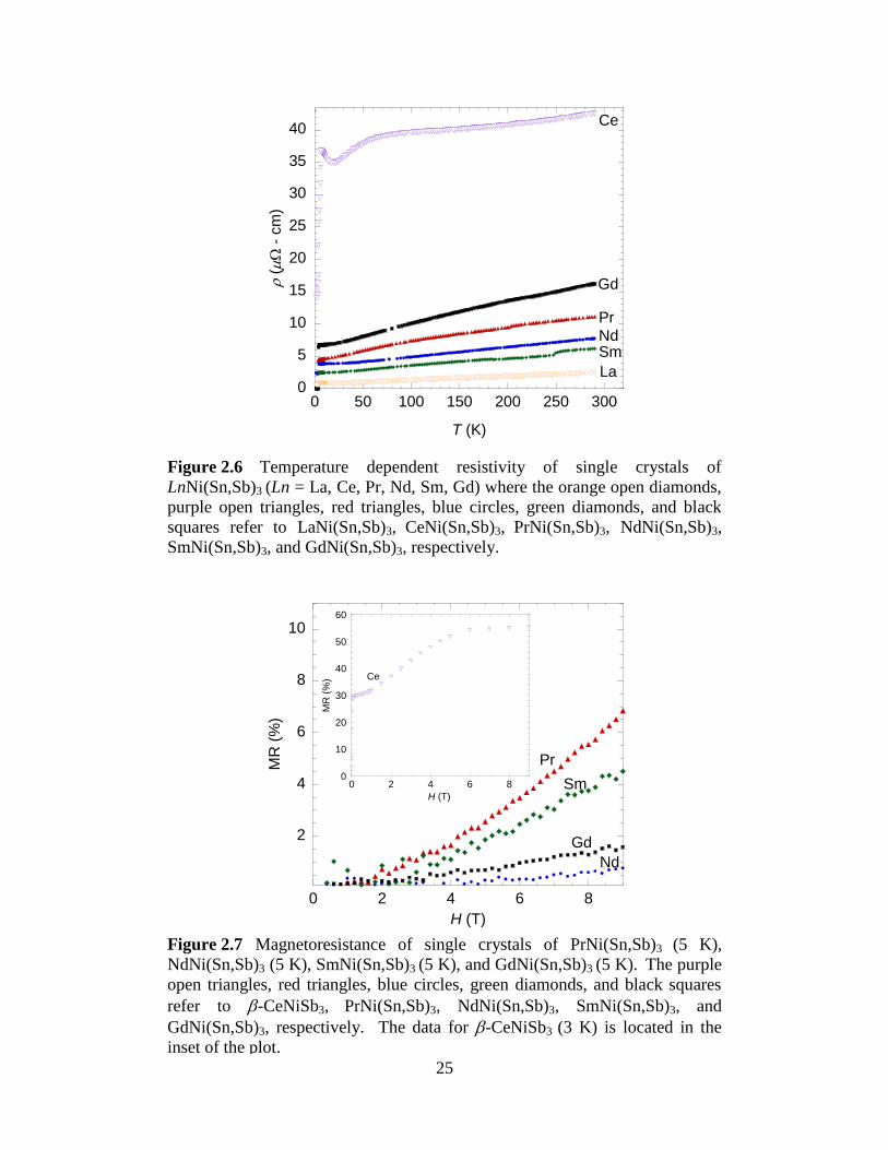
25
2
4
6
8
10
0 2 4 6 8
MR
(%
)
H (T)
Pr
Sm
Gd
Nd
Figure 2.7 Magnetoresistance of single crystals of PrNi(Sn,Sb)3 (5 K),
NdNi(Sn,Sb)3 (5 K), SmNi(Sn,Sb)3 (5 K), and GdNi(Sn,Sb)3 (5 K). The purple
open triangles, red triangles, blue circles, green diamonds, and black squares
refer to -CeNiSb3, PrNi(Sn,Sb)3, NdNi(Sn,Sb)3, SmNi(Sn,Sb)3, and
GdNi(Sn,Sb)3, respectively. The data for -CeNiSb3 (3 K) is located in the
inset of the plot.
0
5
10
15
20
25
30
35
40
0 50 100 150 200 250 300
(
- c
m)
T (K)
Ce
Gd
PrNdSm
La
Figure 2.6 Temperature dependent resistivity of single crystals of
LnNi(Sn,Sb)3 (Ln = La, Ce, Pr, Nd, Sm, Gd) where the orange open diamonds,
purple open triangles, red triangles, blue circles, green diamonds, and black
squares refer to LaNi(Sn,Sb)3, CeNi(Sn,Sb)3, PrNi(Sn,Sb)3, NdNi(Sn,Sb)3,
SmNi(Sn,Sb)3, and GdNi(Sn,Sb)3, respectively.
0
10
20
30
40
50
60
0 2 4 6 8
MR
(%
)
H (T)
Ce

26
La analogue. This indicates that the MR is mostly dominated by the positive contribution,
although one cannot exclude that a small negative contribution, due to the quenching of spin
fluctuations by magnetic field, still persists at low temperatures. Indeed, the MR at H = 9 T
changes sign upon warming and a negative MR is recovered at temperatures above 100 K in all
compounds (not shown). Assuming localized f-electrons, these compounds should have a similar
density of charge carriers. In this case, the difference between the compounds is presumably due
to the interplay between the orbital and the spin contributions. In contrast, the positive MR in the
magnetic phase of CeNi(Sn,Sb)3 at T = 3 K, above the saturation field, also shown in Figure 2.7,
is an order of magnitude larger and saturates around 6 T. The positive non-saturating MR is
reminiscent of other planar materials including structurally related LnSb2 (Ln = La, Pr, Sm, Nd)
whose structure also contains square Sb sheets, however the analogues investigated here have a
significantly smaller magnetoresistance than these other compounds.25
2.4 References
(1) Mills, A. M.; Lam, R.; Ferguson, M. J.; Deakin, L.; Mar, A. Coord. Chem. Rev. 2002,
233-234, 207-222.
(2) Sologub, O.; Salamakha, P. S. Handbook on the Physics and Chemistry of Rare Earths;
Elsevier: Netherlands, 2003; Vol. 33.
(3) Kauzlarich, S. M. Chemistry, Structure, and Bonding in Zintl Phases and Ions; VCH
Publishers: New York, 1996.
(4) Papoian, G. A.; Hoffmann, R. Angew. Chem. Int. Ed. 2000, 39, 2409-2448.
(5) Hartjes, K.; Jeitschko, W.; Brylak, M. J. Magn. Magn. Mater. 1997, 173, 109-116.
(6) Leonard, M.; Saha, S.; Ali, N. J. Appl. Phys. 1999, 85, 4759-4561.
(7) Leonard, M. L.; Dubenko, I. S.; Ali, N. J. Alloys Compd. 2000, 303-304, 265-269.
(8) Jackson, D. D.; Torelli, M.; Fisk, Z. Phys. Rev. B 2001, 65, 014421.
(9) Deakin, L.; Ferguson, M. J.; Mar, A. Chem. Mater. 2001, 13, 1407-1412.

27
(10) Jackson, D. D.; Fisk, Z. J. Magn. Magn. Mater. 2003, 256, 106-116.
(11) Jackson, D. D.; Fisk, Z. J. Alloys Compd. 2004, 377, 243-247.
(12) Deakin, L.; Mar, A. Chem. Mater. 2003, 15, 3343-3346.
(13) Gautreaux, D. P.; Capan, C.; DiTusa, J. F.; Young, D. P.; Chan, J. Y. J. Solid State Chem.
2008, In Press.
(14) Crerar, S. J.; Deakin, L.; Mar, A. Chem. Mater. 2005, 17, 2780-2784.
(15) Macaluso, R. T.; Wells, D. M.; Sykora, R. E.; Albrecht-Schmitt, T. E.; Mar, A.;
Nakatsuji, S.; Lee, H.; Fisk, Z.; Chan, J. Y. J. Solid State Chem. 2004, 177, 293-298.
(16) Siderov, V. A.; Bauer, E. D.; Lee, H.; Nakatsuji, S.; Thompson, J. D.; Fisk, Z. Phys. Rev.
B 2005, 71, 094422-1 - 094422-4.
(17) Thomas, E. L.; Macaluso, R. T.; Lee, H.; Fisk, Z.; Chan, J. Y. J. Solid State Chem. 2004,
177, 4228-4236.
(18) Thomas, E. L.; Moldovan, M.; Young, D. P.; Chan, J. Y. Chem. Mater. 2005, 17, 5810-
5816.
(19) Thomas, E. L.; Gautreaux, D. P.; Lee, H. O.; Fisk, Z.; Chan, J. Y. Inorg. Chem. 2007, 46,
3010-3016.
(20) Thamizhavel, A.; Nakashima, H.; Shiromoto, T.; Obiraki, Y.; Matsuda, T. D.; Haga, Y.;
Ramakrishnan, S.; Takeuchi, T.; Settai, R.; Onuki, Y. J. Phys. Soc. Jpn. 2005, 74, 2617-
2621.
(21) Thomas, E. L.; Gautreaux, D. P.; Chan, J. Y. Acta Crystallogr. Sect. E: Struct. Rep.
Online 2006, E62, i96-i98.
(22) Sheldrick, G. M.; University of Gottingen: Germany, 1997.
(23) Lee, H.-O.; Nakatsuji, S.; Chen, Y.; Bao, W.; Hundley, M. F.; Macaluso, R. T.; Chan, J.
Y.; Carter, B.; Klavins, P.; Schlottmann, P.; Fisk, Z.
(24) Jensen, J.; Mackintosh, A. R. Rare Earth Magnetism Structure and Excitations;
Clarendon Press: Oxford, 1991.
(25) Bud'ko, S. L.; Canfield, P. C.; Mielke, C. H.; Lacerda, A. H. Phys. Rev. B 1998, 57,
13624-13638.

28
CHAPTER 3 – CeNixCo1-xSb3
3.1 Introduction
Doping is a method of introducing an element into a known compound to modify the
compound’s physical properties and structure. Co is one of the five naturally occurring
ferromagnetic elements and has a Curie temperature of 1388 K.1 Fe and Ni are also
ferromagnetic below their Curie temperatures of 1043 K and 627 K respectively.1 Lanthanide –
cobalt compounds have also demonstrated a phenomenon known as itinerant electron
metamagnetism (IEM) where a first order transition from a nonmagnetic state to a ferromagnetic
state occurs.3 This transition is caused by the ordering of the Co sublattice and generally occurs
in addition to the local magnetic moment caused by the rare earth element.4 FeSi, a narrow-gap
semiconductor has been doped with Co to produce a compound with extraordinary
magnetoconductance.5 Another study showed that when FeSi is doped with Co a Curie
temperature of 53 K is obtained along with a very high Hall conductance which are important
developments for spintronics materials.6 By substituting Co for Ni in -CeNiSb3, the number of
carriers might change which can affect the magnetic or transport behavior. The crystal growth
and structure as well as physical properties of CeNixCo1-xSb3 are reported herein.
3.2 Experimental
3.2.1 Synthesis
Single crystals of CeNixCo1-xSb3, where x = 0.8, were prepared using an excess Sb flux
growth method. Ce ingot (99.9%, Alfa Aesar), Ni powder (99.999%, Alfa Aesar), Co powder
(99.999%, Alfa Aesar), and Sb shot (99.999%, Alfa Aesar) were placed in an alumina crucible in
a 1:0.8:0.2:20 molar ratio. The crucible was sealed into an evacuated fused-silica tube. The
2 Portions of this chapter reprinted by permission of Elsevier: Gautreaux, D.P.; Parent, M.; Moldovan, M.;
Young, D.P.; Chan, J.Y.; “Magnetization and Transport Properties of CeNi0.78Co0.22Sb3”, Physica B. 2008, 403,
5-9.
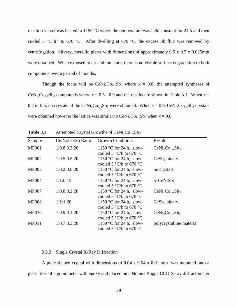
29
reaction vessel was heated to 1150 °C where the temperature was held constant for 24 h and then
cooled 5 °C h-1
to 670 °C. After dwelling at 670 °C, the excess Sb flux was removed by
centrifugation. Silvery, metallic plates with dimensions of approximately 0.5 x 0.5 x 0.025mm
were obtained. When exposed to air and moisture, there is no visible surface degradation to both
compounds over a period of months.
Though the focus will be CeNixCo1-xSb3 where x = 0.8, the attempted syntheses of
CeNixCo1-xSb3 compounds where x = 0.5 - 0.9 and the results are shown in Table 3.1. When x =
0.7 or 0.5, no crystals of the CeNixCo1-xSb3 were obtained. When x = 0.9, CeNixCo1-xSb3 crystals
were obtained however the lattice was similar to CeNixCo1-xSb3 when x = 0.8.
Table 3.1 Attempted Crystal Growths of CeNixCo1-xSb3
Sample Ce:Ni:Co:Sb Ratio Growth Conditions Result
MP001 1:0.8:0.2:20 1150 °C for 24 h, slow- CeNixCo1-xSb3
cooled 5 °C/h to 670 °C
MP002 1:0.5:0.5:20 1150 °C for 24 h, slow- CeSb2 binary
cooled 5 °C/h to 670 °C
MP003 1:0.2:0.8:20 1150 °C for 24 h, slow- no crystals
cooled 5 °C/h to 670 °C
MP004 1:1:0:15 1150 °C for 24 h, slow- -CeNiSb3
cooled 5 °C/h to 670 °C
MP007 1:0.8:0.2:20 1150 °C for 24 h, slow- CeNixCo1-xSb3
cooled 5 °C/h to 670 °C
MP008 1:1:1:20 1150 °C for 24 h, slow- CeSb2 binary
cooled 5 °C/h to 670 °C
MP010 1:0.9:0.1:20 1150 °C for 24 h, slow- CeNixCo1-xSb3
cooled 5 °C/h to 670 °C
MP011 1:0.7:0.3:20 1150 °C for 24 h, slow- polycrystalline material
cooled 5 °C/h to 670 °C
3.2.2 Single Crystal X-Ray Diffraction
A plate-shaped crystal with dimensions of 0.04 x 0.04 x 0.01 mm3 was mounted onto a
glass fiber of a goniometer with epoxy and placed on a Nonius Kappa CCD X-ray diffractometer
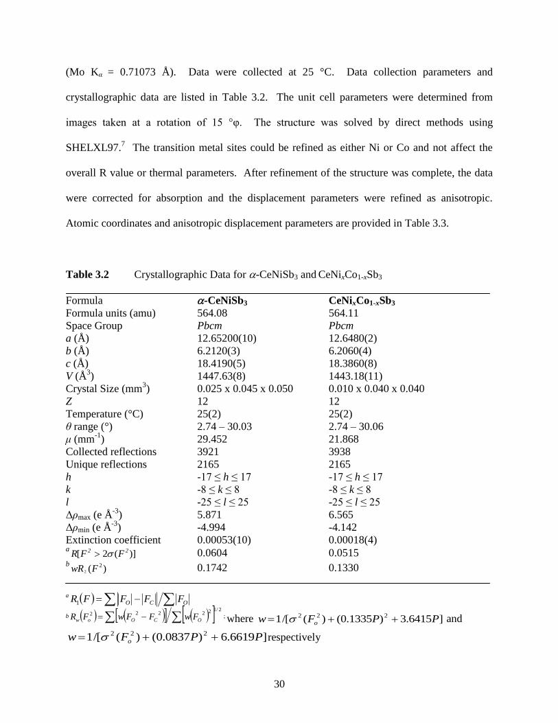
30
(Mo Kα = 0.71073 Å). Data were collected at 25 °C. Data collection parameters and
crystallographic data are listed in Table 3.2. The unit cell parameters were determined from
images taken at a rotation of 15 °φ. The structure was solved by direct methods using
SHELXL97.7 The transition metal sites could be refined as either Ni or Co and not affect the
overall R value or thermal parameters. After refinement of the structure was complete, the data
were corrected for absorption and the displacement parameters were refined as anisotropic.
Atomic coordinates and anisotropic displacement parameters are provided in Table 3.3.
Table 3.2 Crystallographic Data for -CeNiSb3 and CeNixCo1-xSb3
Formula -CeNiSb3 CeNixCo1-xSb3
Formula units (amu) 564.08 564.11
Space Group Pbcm Pbcm
a (Å) 12.65200(10) 12.6480(2)
b (Å) 6.2120(3) 6.2060(4)
c (Å) 18.4190(5) 18.3860(8)
V (Å3) 1447.63(8) 1443.18(11)
Crystal Size (mm3) 0.025 x 0.045 x 0.050 0.010 x 0.040 x 0.040
Z 12 12
Temperature (°C) 25(2) 25(2)
θ range (°) 2.74 – 30.03 2.74 – 30.06
μ (mm-1
) 29.452 21.868
Collected reflections 3921 3938
Unique reflections 2165 2165
h -17 ≤ h ≤ 17 -17 ≤ h ≤ 17
k -8 ≤ k ≤ 8 -8 ≤ k ≤ 8
l -25 ≤ l ≤ 25 -25 ≤ l ≤ 25
Δρmax (e Å-3
) 5.871 6.565
Δρmin (e Å-3
) -4.994 -4.142
Extinction coefficient 0.00053(10) 0.00018(4) a
)](2[ 22 FFR 0.0604 0.0515 b
)( 22 FwR
0.1742 0.1330
a OCO FFFFR1
b 2/122222 OCOow FwFFwFR ; where ]6415.3)1335.0()(/[1 222 PPFw o and
]6619.6)0837.0()(/[1 222 PPFw o respectively

31
Table 3.3 Atomic Positions and Displacement Parameters for CeNixCo1-xSb3
Atom Wyckoff site x y z Ueq (Å2)a
Ce1 4d 0.30507(7) 0.55270(16) ¼ 0.0089(2)
Ce2 8e 0.29910(5) 0.02420(11) 0.41677(3) 0.0084(2)
M1b 4c 0.89836(16) ¼ ½ 0.0105(4)
M2b 8e 0.90174(12) 0.8252(3) 0.17577(9) 0.0116(4)
Sb1 8e 0.50321(5) 0.78945(13) 0.33405(4) 0.0097(2)
Sb2 4d 0.21816(8) 0.04743(19) ¼ 0.0096(3)
Sb3 4c 0.50359(8) ¼ ½ 0.0102(3)
Sb4 8e 0.22288(6) 0.52308(13) 0.41567(4) 0.0091(2)
Sb5 8e 0.97368(6) 0.54075(13) 0.41329 0.0116(2)
Sb5 4d 0.07541(8) 0.68314(18) ¼ 0.0110(3)
aUeq is defined as one-third of the trace of the orthogonalized Uij tensor.
bM1 and M2 represent a mixture of Ni and Co
3.2.3 ICP-Optical Emission Spectroscopy
Elemental analysis of CeNixCo1-xSb3 using inductively coupled plasma-optical emission
spectroscopy (ICP-OES) was performed at Galbraith Laboratories. This analysis was performed
due to the similar X-ray scattering of Ni and Co. X-ray diffraction cannot distinguish between
elements with similar Z. Optical emission spectroscopy excites each of the atoms present and
upon relaxation light is emitted and with a polychromatic detector, the amount of each element
present can be determined. This analysis was performed for Ni and Co and a stoichiometry of
CeNi0.780Co0.220Sb3 was obtained. This is similar to the nominal composition of
CeNi0.80Co0.20Sb3.
3.2.4 Physical Property Measurements
Magnetic susceptibility data (between 2 K – 300 K) at an applied field of 0.1 T and
magnetization (up to 9 T) at 3 K were measured using a Quantum Design Physical Property
Measurement System (PPMS). The resistivity (between 2 K - 300 K) was measured on a single
crystal using the standard four wires and AC lock-in techniques (with thin Pt wires attached

32
using silver epoxy) in a Quantum Design Physical Property Measurement System (PPMS) at
ambient pressure.
3.3 Results and Discussion
3.3.1 Structure
CeNi0.80Co0.20Sb3 crystallizes in the CeNiSb3 structure type.8 The structure of
CeNi0.80Co0.20Sb3 is shown in Figure 3.1. The structure consists of layers of mono-capped square
anti-prismatic CeSb9 above and below a layer of Sb square nets. Layers of distorted face- and
edge- sharing MSb6 octahedra are located between the CeSb9 layers. The transition metal site
will be referred to as M1 and M2 which will be a mixture of Ni and Co on each site. Figure 3.2
shows the X-ray powder patterns of CeNixCo1-xSb3 and -CeNiSb3. Each reflection is indexed
according to the structural data from single crystal X-ray diffraction. The atomic radius of Co is
slightly larger than that of Ni so a peak shift to the left is expected and observed. The second
Figure 3.1 The structure of CeNixCo1-xSb3 viewed down the b-axis. The
yellow spheres represent Ce atoms, blue and green spheres represent Ni/Co
atoms, and maroon spheres represent Sb atoms.
Ce1 Ce2
a
c

33
pattern in Figure 3.2 displays the 400 reflection and the slight shift once Co is introduced into the
-CeNiSb3 structure type.
3.3.2 Physical Properties
The magnetic susceptibility ( vs T) measured at an applied field of 0.2 T for 10 mg of
single crystals of CeNi0.78Co0.22Sb3 is shown in Figure 3.3. The magnetic field is oriented along
the c-axis of the crystals. A ferromagnetic transition is observed at ~ 4.6 K which is lower than
the 6 K ordering temperature of the -CeNiSb3.9 Although the Ni atoms in pure CeNiSb3 do not
contribute directly to the magnetism, the insertion of Co into this sublattice may disrupt the
overall magnetic moment. From the inverse susceptibility versus temperature plot from 50 K –
150 K, the experimental effective moment of 2.43 B/Ce and a Weiss temperature () of 41 K
were obtained. The eff of 2.43 B is close to the calculated 2.54 B for the Ce3+
ion.1 This is
consistent with the magnetic contribution due solely to the Ce3+
. The average effective moment
of -CeNiSb3 is 2.58B/Ce and the values for the Weiss constant, , are -156 along the ab plane
and 29 K along the c-axis.9
The magnetization as a function of vield (M vs H) measured at 3 K on the same sample
40
0
40
2
40
00
20
02
0 31
33
13
22
02
06
41
34
13
50
05
00
32
0 30
63
06
02
6
22
0
20
6
40
0
40
2
40
00
20
02
0 31
33
13
22
02
06
41
34
13
50
05
00
32
0 30
63
06
02
6
22
0
20
6
2 (°) 2 (°)
Inte
nsi
ty
40
0
CeNixCo1-xSb3
α-CeNiSb3
Space Group: Pbcm
Lattice ~ 12 x 6 x 18
Figure 3.2 X-ray diffraction powder patterns of CeNixCo1-xSb3 and α-
CeNiSb3. The pattern on the left is the full spectrum for each compound and
the pattern to the right displays the shift seen in the 400 peak.

34
of CeNi0.78Co0.22Sb3 is shown in Figure 3.4. At H ~ 1 T, the magnetization begins to show signs
of slow saturation well below the theoretical saturation moment of 2.14 B for Ce3+
. A similar
result is observed in the pure material, which has a large magnetocrystalline anisotropy and
shows evidence for a modest Kondo interaction, with the ground state being a crystal-field-split
doublet of Ce.9
0
0.2
0.4
0.6
0.8
1
0 5 10 15 20T (K)
M/H
(em
u/m
ol C
e)
0.00
0.05
0.10
0.15
0.20
0.25
0.30
0.35
0 2 4 6 8 10
M (
B/m
ol-
Ce
)
H (T)
Figure 3.3 The magnetic susceptibility (M vs T) measured at an applied
field of 0.2 T of CeNi0.780Co0.220Sb3.
Figure 3.4 The magnetization as a function of field (M vs H) measured at 3
K of CeNi0.780Ce0.220Sb3.

35
50
55
60
65
70
75
0 50 100 150 200 250 300T (K)
-cm
The resistivity as a function of temperature for a single crystal of CeNi0.78Co0.22Sb3 is
shown in Figure 3.5. The current has been applied along the b-axis (in-plane). The overall shape
of the curve is similar to that of -CeNiSb38 and is weakly temperature dependent and
characteristic of Kondo systems. However, the minimum observed near 27 K is much deeper
here than it is for pure CeNiSb3, which could be due to more Kondo-like behavior of the doped
sample. This effect is analogous to the physical pressure effects observed in another Kondo
lattice system, CeAl2.10
Below ~ 5 K (Tc) the resistivity decreases very quickly, in response to
the reduction in the spin disorder scattering.
The magnetoresistance at 3 K of CeNi0.78Co0.22Sb3 is shown in Figure 3.6. Unlike usual
ferromagnets, the magnetoresistance is positive, increasing to over 10% by 9 T. The shape of the
magnetoresistance essentially tracks the magnetization of the sample for the field applied along
the same direction which may be due to the magnetic anisotropy of the crystal.
Figure 3.5 The resistivity of CeNi0.780Co0.220Sb3 measured between 2 and
290 K.

36
0
2
4
6
8
10
12
0 2 4 6 8 10
x
10
0 (
%)
H (T)
T = 3K
The slightly lower ferromagnetic ordering temperature, smaller saturation moment, and
deeper minimum in the resistivity data summarize the effects of Co substitution on pure CeNiSb3
for this concentration.
3.4 References
(1) Kittel, C.; 7th ed.; John Wiley & Sons, Inc.: New York, 1995.
(2) Gautreaux, D. P.; Parent, M.; Moldovan, M.; Young, D. P.; Chan, J. Y. Physica B 2008,
403, 1005-1006.
(3) Duc, N. H.; Goto, T. Handbook on the Physics and Chemistry of Rare Earths; Elsevier
Science: Netherlands, 1999; Vol. vol. 26.
(4) Duc, N. H.; Hien, T. D.; Brommer, P. E.; Franse, J. J. M. J. Magn. Magn. Mater. 1992,
104-107, 1252.
(5) Manyala, N.; Sidis, Y.; DiTusa, J. F.; Aeppli, G.; Young, D. P.; Fisk, Z. Nature 2000,
404, 581-584.
(6) Manyala, N.; Sidis, Y.; DiTusa, J. F.; Aeppli, G.; Young, D. P.; Fisk, Z. Nature Mater.
2004, 3, 255-262.
Figure 3.6. The magnetoresistance of CeNi0.780Ce0.220Sb3 at 3 K taken from 0
to 9 T.
37
(7) Sheldrick, G. M.; University of Gottingen: Germany, 1997.
(8) Macaluso, R. T.; Wells, D. M.; Sykora, R. E.; Albrecht-Schmitt, T. E.; Mar, A.;
Nakatsuji, S.; Lee, H.; Fisk, Z.; Chan, J. Y. J. Solid State Chem. 2004, 177, 293-298.
(9) Siderov, V. A.; Bauer, E. D.; Lee, H.; Nakatsuji, S.; Thompson, J. D.; Fisk, Z. Phys. Rev.
B 2005, 71, 094422-1 - 094422-4.
(10) Nicolas-Francillon, M.; Percheron, A.; Achard, J. C. Solid State Comm. 1972, 11, 845-
849.
38
CHAPTER 4 – Ln(Cu1-xNix)ySb2
4.1 Introduction
Antimonide compounds have been a focus of many research groups because of the
interesting structural features and physical properties they possess.1-4
All analogues of LnSb2 (Ln
= La – Nd, Sm) show positive, linear magnetoresistance at 2 K.5 Also of notable interest is
LaSb2, which has a positive, linear magnetoresistance below 10 K greater that 8,500 % with no
signs of saturation up to 45 T.6 Adopting a similar layered structure, LnNi1-xSb2 (Ln = Y, Dy,
and Ho) analogues have large positive magnetoresistance above 100 % at 3 K.7 Single
crystalline CeNiSb2 is reported to order ferromagnetically at 6 K and has a Sommerfeld
coefficient (γ) of 55 mJ mol-1
K-2
.8 It is important to note that the full structural determination
has not been reported for CeNiSb2 and the physical properties are similar to the fully
characterized orthorhombic CeNiSb3 which orders ferromagnetically at 6 K and has a
Sommerfeld coefficient (γ) of ~50 mJ mol-1
K-2
.4,9
CeMSb2 (M = Ni, Cu, Pd, and Ag) show
dense Kondo behavior and polycrystalline CeNiSb2 shows an enhanced electron mass.10
The
magnetoresistance of polycrystalline CeCuSb2 has been reported to be ~12.5 % at 4.5 T and 4.5
K.11
CeCuSb2, both in the polycrystalline and single-crystalline form, orders
antiferromagnetically between 7 – 8 K.8,10,12-15
CeCuSb2 is also a heavy fermion with reported
Sommerfeld coefficients (γ) of 94, 100, and 200 mJ mol-1
K-2
.8,10,14,15
In an effort to further determine structural stability of ternary Ce – Ni – Sb and Ce – Cu –
Sb compounds, single crystals of various compositions of Ce(Cu1-xNix)ySb2 were obtained. The
crystal structure, elemental analysis, magnetic and transport properties of Ce(Cu1-xNix)ySb2 (x =
0, 0.25, 0.37, and 0.46) are reported herein.
39
4.2 Experimental
4.2.1 Synthesis
High quality single crystals of Ln(Cu1-xNix)ySb3 were synthesized via flux growth by
placing fragments of La or Ce rod (99.9% Alfa Aesar), Ni powder (99.999% Alfa Aesar), Cu
powder (99.999% Alfa Aesar) and Sb shot (99.999% Alfa Aesar) in an alumina crucible. The
nominal composition used was 1 : x : 1-x : 20 (x = 0, 0.6, 0.7, 0.8) for Ce : Ni : Cu : Sb, where
excess Sb was included as the flux. For the La analogue, the nominal composition of 1 : 0.8 : 0.2
: 20 for La : Ni : Cu : Sb was used. Silica wool was placed on top of the crucible and was sealed
under vacuum in a fused silica tube and placed in a furnace. The reaction vessel was heated to
1150 ºC and held constant for 48 hours, then cooled to 670 C at a rate of 5 ºC h-1
. Excess flux
was removed by centrifugation. Single crystals were extracted with sizes up to 0.5 x 1 x 2 mm3
although the crystals tend to grow into larger, layered aggregates. The tetragonal plates are
silver with a metallic luster. However, at lower concentrations of Cu, crystals gain a dull, blue-
gray iridescence and begin to resemble crystals of CeNiSb3.4 The crystals are stable in air over a
period of months. It is important to note that under our growth conditions, where the nominal
value of x > 0.8, single crystals of CeNiSb3 were grown. This will be discussed more in depth in
the structural analysis section.
4.2.2 Single Crystal X-Ray Diffraction
A typical crystal with dimensions of ~ 0.05 x 0.10 x 0.175 mm3 was mounted onto a glass
fiber of a goniometer with epoxy and placed on a Nonius Kappa CCD X-ray diffractometer
(MoKα = 0.71073 Å). After choosing the tetragonal space group P4/nmm (No. 129), the initial
structural model was generated by SIR9716
and the model was then refined by direct methods
using SHELXL97.17
Due to the similarity of Z for Ni and Cu, X-rays cannot accurately
distinguish between the two. Therefore, the mixed transition metal site was refined as pure Cu
40
for continuity and is designated as M. After refinement, the data were corrected for absorption
and the displacement parameters were refined as anisotropic. An extinction coefficient was
added and refined through multiple least squares cycles. A disagreeable thermal parameter for
the transition metal site was observed and the site was allowed to be partially occupied. This is
consistent with the partial transition metal occupancy observed in most other analogues of the
HfCuSi2 structure type. For simplicity, the exact partial occupancy will not be defined in the text
for each compound as each value differs. It will be designated as y and the exact values will be
listed in the crystallographic tables. Data collection parameters and crystallographic data are
listed in Table 4.1. Atomic coordinates, anisotropic displacement parameters, and site
occupancies are provided in Table 4.2.
4.2.3 Energy Dispersive Spectroscopy
Elemental analysis was performed on multiple single crystalline samples using the
Hitachi S-3600N extra-large chamber variable pressure Scanning Electron Microscope (VP-
SEM) with an integrated energy dispersive (EDS) feature. Data were collected over a small flux-
free area on the surface of the crystals using an accelerating voltage of 20 kV and 50 s
acquisition times. This analysis was performed due to the similar X-ray scattering of Ni and Cu.
X-ray diffraction cannot distinguish between elements with similar Z and it is important to know
the exact amounts of Ni and Cu in the sample. The transition metal site occupancy is consistent
with the occupancy determined from single crystal X-ray diffraction data and formula
compositions are located in Table 4.3. Is is important to note that the nominal and exact Ni/Cu
concentrations do not agree, however there is a systematic increase of Ni in both the nominal and
exact compositions. From this point on, the actual EDS compositions will be used.
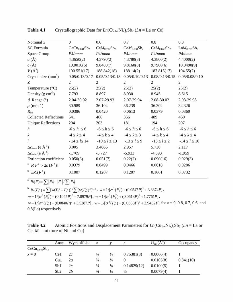
41
Table 4.1 Crystallographic Data for Ln(Cu1-xNix)ySb2 (Ln = La or Ce)
Nominal x 0 0.6 0.7 0.8 0.8
SC Formula CeCu0.841Sb2 CeM0.707Sb2 CeM0.738Sb2 CeM0.665Sb2 LaM0.779Sb2
Space Group P4/nmm P4/nmm P4/nmm P4/nmm P4/nmm
a (Å) 4.3650(2) 4.3790(2) 4.3780(3) 4.3800(2) 4.4000(2)
c (Å) 10.0010(6) 9.8480(7) 9.8160(8) 9.7900(6) 10.0490(9)
V (Å3) 190.551(17) 188.842(18) 188.14(2) 187.815(17) 194.55(2)
Crystal size (mm3) 0.05/0.13/0.17 0.05/0.13/0.13 0.05/0.10/0.13 0.08/0.13/0.15 0.05/0.08/0.10
Z 2 2 2 2 2
Temperature (°C) 25(2) 25(2) 25(2) 25(2) 25(2)
Density (g cm-1
) 7.793 8.897 8.930 8.945 8.615
Range (°) 2.04-30.02 2.07-29.93 2.07-29.94 2.08-30.02 2.03-29.98
μ (mm-1) 30.989 36.104 36.239 36.302 34.326
Rint 0.0386 0.0420 0.0613 0.0379 0.0360
Collected Reflections 541 466 356 489 460
Unique Reflections 204 203 181 194 207
h -6 h 6 -6 h 6 -6 h 6 -6 h 6 -6 h 6
k -4 k 4 -4 k 4 -4 k 3 -4 k 4 -4 k 4
l - 14 l 14 -10 l 13 -13 l 9 -13 l 2 -14 l 10
max (e Å-3
) 3.005 3.4666 2.957 5.730 2.117
min (e Å-3
) -1.709 -5.727 -5.933 -4.593 -1.959
Extinction coefficient 0.050(6) 0.051(7) 0.22(2) 0.090(16) 0.029(3) a )](2[ 22 FFR 0.0379 0.0499 0.0466 0.0618 0.0286
b )( 2
2 FwR 0.1007 0.1207 0.1207 0.1661 0.0732
a 001 /)( FFFFR c
b 2/122
0
22
0
2
0 ])([/)]([)( FwFFwFR cw ; ]3374.3)0547.0()(/[1 22
0
2 PPFw ,
]0979.7)1045.0()(/[1 22
0
2 PPFw , ]7761.1)0613.0()(/[1 22
0
2 PPFw ,
]5287.3)0840.0()(/[1 22
0
2 PPFw , ]9432.3)0358.0()(/[1 22
0
2 PPFw for x = 0, 0.8, 0.7, 0.6, and
0.8(La) respectively
Table 4.2 Atomic Positions and Displacement Parameters for Ln(Cu1-xNix)ySb2 (Ln = La or
Ce, M = mixture of Ni and Cu)
Atom Wyckoff site x y z Ueq (Å2)
a Occupancy
CeCu0.841Sb2
x = 0 Ce1 2c ¼ ¼ 0.75381(8) 0.0066(4) 1
Cu1 2a ¾ ¼ 0 0.0103(8) 0.841(10)
Sb1 2c ¼ ¼ 0.14829(12) 0.0100(5) 1
Sb2 2b ¾ ¼ ½ 0.0079(4) 1

42
Table 4.2 (cont.)
Atom Wyckoff site x y z Ueq (Å2)
a Occupancy
CeM0.665Sb2
x = 0.8 Ce1 2c ¼ ¼ 0.75909(15) 0.0073(8) 1
M1 2a ¾ ¼ 0 0.0063(14) 0.665(17)
Sb1 2c ¼ ¼ 0.1367(8) 0.0136(8) 1
Sb2 2b ¾ ¼ ½ 0.0091(8) 1
CeM0.738Sb2
x = 0.7 Ce1 2c ¼ ¼ 0.24163(9) 0.0062(6) 1
M1 2a ¾ ¼ 0 0.0103(10) 0.738(10)
Sb1 2c ¼ ¼ 0.86089(13) 0.0123(7) 1
Sb2 2b ¾ ¼ ½ 0.0075(7) 1
CeM0.707Sb2
x = 0.6 Ce1 2c ¼ ¼ 0.75771(11) 0.0081(6) 1
M1 2a ¾ ¼ 0 0.0083(10) 0.707(11)
Sb1 2c ¼ ¼ 0.14063(16) 0.0139(6) 1
Sb2 2b ¾ ¼ ½ 0.0092(6) 1
LaM0.779Sb2
x = 0.8 La1 2c ¼ ¼ 0.75641(11) 0.0067(4) 1
M1 2a ¾ ¼ 0 0.0091(9) 0.779(10)
Sb1 2c ¼ ¼ 0.13948(14) 0.0129(4) 1
Sb2 2b ¾ ¼ ½ 0.0082(4) 1 aUeq is defined as one-third of the trace of the orthogonalized Uij tensor.
Table 4.3 EDS Formula Compositions for Ce(Cu1-xNix)ySb2
Nominal Composition Single Crystal Formula EDS Formula
x = 0.8 Ce(M)0.665Sb2 Ce(Ni0.46Cu0.54)0.67Sb2.16
x = 0.7 Ce(M)0.738Sb2 Ce(Ni0.37Cu0.63)0.74Sb1.86
x = 0.6 Ce(M)0.707Sb2 Ce(Ni0.25Cu0.75)0.69Sb2.16
4.2.4 Physical Property Measurements
Magnetic measurements on single crystals of Ce(Cu1-xNix)ySb2 oriented in the same
direction were performed using a Quantum Design Physical Property Measurement System
(PPMS). Temperature-dependent susceptibility data were measured with an applied field of 0.1
T from 2 K to 300 K. Magnetization as a function of field was measured at 3 K up to 9 T. The

43
resistivity from 2 K – 300K and magnetoresistance at 3 K (up to 9 T) were measured using the
standard four probe-AC method in the Quantum Design PPMS at ambient pressure.
4.3 Results and Discussion
4.3.1 Structural Changes
Ln(Cu1-xNix)ySb2 (Ln = La, Ce) crystallizes in the tetragonal space group P4/nmm with
the HfCuSb2 structure type.18
As indicated in Tables 4.1 and 4.3, the nominal and exact
compositions of Ni and Cu do not agree. However, there is a systematic increase of Ni in both
the nominal and exact compositions. For consistency throughout this document, the compounds
will be referred to by their actual compositions. We believe that there is a limit to the amount of
Ni that can occupy the transition metal site when there is a large rare earth cation such as Ce
present in the structure under our growth conditions. When too much Ni is added to the reaction
mixture, the tetragonal structure can no longer be supported and the stable phase that forms is the
CeNiSb3 structure type.4 This theory is supported by earlier work where pure LnNiSb2 can only
be formed in the presence of smaller rare earth cations (Gd – Er, Y).7 In the presence of larger
rare earth ions such as Ce – Sm, the orthorhombic LnNiSb3 structure is formed using the Sb flux
growth method.4,19
We note that other experimental techniques such as arc-melting have yielded
LnNiSb2 (Ln = Pr, Nd, Sm).12
As previously stated, Ln(Cu1-xNix)ySb2 (Ln = La, Ce) crystallizes in the tetragonal space
group P4/nmm. The structure consists of alternating layers of Sb2 square nets capped by Ln1
square antiprismatic layers and M1-Sb1 tetrahedral layers as shown in Figure 4.1. The Ln atoms
are coordinated to four Sb1 atoms from the M tetrahedral layer and four Sb2 atoms from the net
layer, forming a slightly distorted square antiprism. The M atoms are surrounded by four Sb1
atoms adopting a somewhat distorted tetrahedral geometry. This layered antimonide structure is
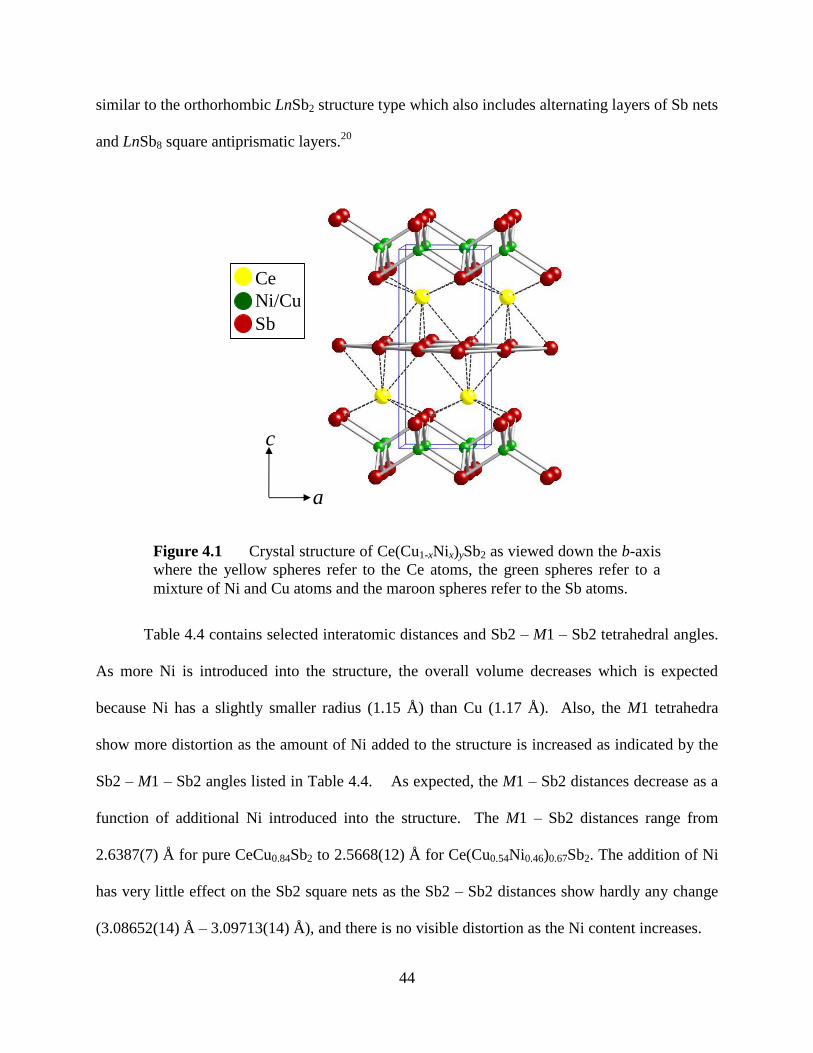
44
similar to the orthorhombic LnSb2 structure type which also includes alternating layers of Sb nets
and LnSb8 square antiprismatic layers.20
Table 4.4 contains selected interatomic distances and Sb2 – M1 – Sb2 tetrahedral angles.
As more Ni is introduced into the structure, the overall volume decreases which is expected
because Ni has a slightly smaller radius (1.15 Å) than Cu (1.17 Å). Also, the M1 tetrahedra
show more distortion as the amount of Ni added to the structure is increased as indicated by the
Sb2 – M1 – Sb2 angles listed in Table 4.4. As expected, the M1 – Sb2 distances decrease as a
function of additional Ni introduced into the structure. The M1 – Sb2 distances range from
2.6387(7) Å for pure CeCu0.84Sb2 to 2.5668(12) Å for Ce(Cu0.54Ni0.46)0.67Sb2. The addition of Ni
has very little effect on the Sb2 square nets as the Sb2 – Sb2 distances show hardly any change
(3.08652(14) Å – 3.09713(14) Å), and there is no visible distortion as the Ni content increases.
a
c
Ce
Ni/Cu
Sb
Figure 4.1 Crystal structure of Ce(Cu1-xNix)ySb2 as viewed down the b-axis
where the yellow spheres refer to the Ce atoms, the green spheres refer to a
mixture of Ni and Cu atoms and the maroon spheres refer to the Sb atoms.
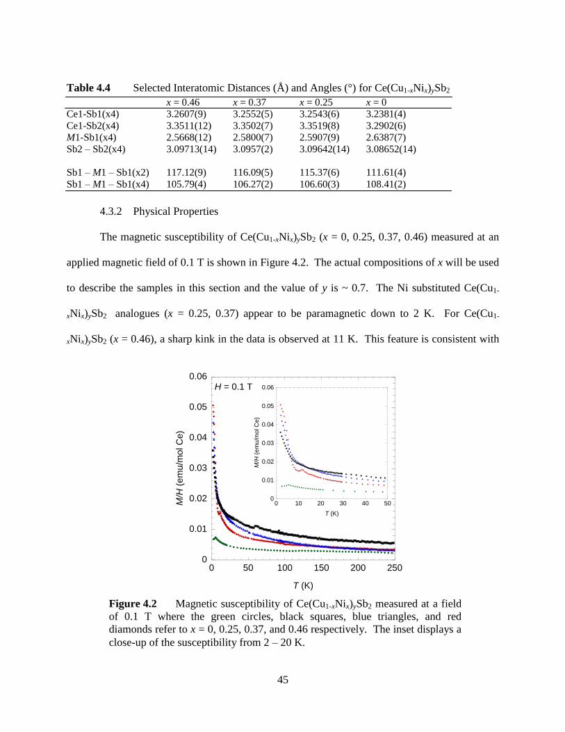
45
Table 4.4 Selected Interatomic Distances (Å) and Angles (°) for Ce(Cu1-xNix)ySb2
x = 0.46 x = 0.37 x = 0.25 x = 0
Ce1-Sb1(x4) 3.2607(9) 3.2552(5) 3.2543(6) 3.2381(4)
Ce1-Sb2(x4) 3.3511(12) 3.3502(7) 3.3519(8) 3.2902(6)
M1-Sb1(x4) 2.5668(12) 2.5800(7) 2.5907(9) 2.6387(7)
Sb2 – Sb2(x4) 3.09713(14) 3.0957(2) 3.09642(14) 3.08652(14)
Sb1 – M1 – Sb1(x2) 117.12(9) 116.09(5) 115.37(6) 111.61(4)
Sb1 – M1 – Sb1(x4) 105.79(4) 106.27(2) 106.60(3) 108.41(2)
4.3.2 Physical Properties
The magnetic susceptibility of Ce(Cu1-xNix)ySb2 (x = 0, 0.25, 0.37, 0.46) measured at an
applied magnetic field of 0.1 T is shown in Figure 4.2. The actual compositions of x will be used
to describe the samples in this section and the value of y is ~ 0.7. The Ni substituted Ce(Cu1-
xNix)ySb2 analogues (x = 0.25, 0.37) appear to be paramagnetic down to 2 K. For Ce(Cu1-
xNix)ySb2 (x = 0.46), a sharp kink in the data is observed at 11 K. This feature is consistent with
0
0.01
0.02
0.03
0.04
0.05
0.06
0 50 100 150 200 250
T (K)
M/H
(e
mu
/mo
l C
e)
H = 0.1 T
Figure 4.2 Magnetic susceptibility of Ce(Cu1-xNix)ySb2 measured at a field
of 0.1 T where the green circles, black squares, blue triangles, and red
diamonds refer to x = 0, 0.25, 0.37, and 0.46 respectively. The inset displays a
close-up of the susceptibility from 2 – 20 K.
0
0.01
0.02
0.03
0.04
0.05
0.06
0 10 20 30 40 50
T (K)
M/H
(e
mu
/mol C
e)

46
the onset of long-range antiferromagnetic order. CeCu0.84Sb2 (x = 0) orders
antiferromagnetically at ~ 6 K which is consistent with literature reports.8,10,12-15
The effective
moments for each sample were calculated using a modified Curie-Weiss equation, χ = χ0 + C/(T -
θ), where χ is the magnetic susceptibility, χ0 is the temperature-independent contribution, C is the
Curie constant, T is the temperature, and θ is the Weiss constant. Experimental effective
moments of 2.32 µB, 2.44 µB, 2.38 µB, and 2.31 µB were calculated for compounds with x = 0.46,
0.37, 0.25, and 0 respectively, and all are in agreement with the calculated moment of 2.54 µB
for the free Ce3+
ion. Curie temperatures of ~ -62, -35, -25, and -225 were observed for
compounds with x = 0.46, 0.37, 0.25, and 0, respectively and indicate that there are
antiferromagnetic correlations within the structures. A summary of the magnetic data are located
in Table 4.5.
Table 4.5 Summary of Magnetic Data for Ce(Cu1-xNix)ySb2 (x = 0.8, 0.7, 0.6, and 0)
xa 0.46 0.37 0.25 0
Fit Range 50 – 275 K 50 – 275 K 100 – 275 K 75 – 250 K
TN (K) 11 - - 8
χ0 0.00125 0.000578 0.00296 0.00102
C 0.6716 0.7455 0.7058 0.6685
θ (K) -62.54 -34.593 -24.72 -225.17
μcalc (μB) 2.32 2.44 2.38 2.31
μeff (μB) 2.54 2.54 2.54 2.54 ax = composition as obtained from elemental analysis
The magnetization of Ce(Cu1-xNix)ySb2 (x = 0.46, 0.37, 0.25, and 0) as a function of field
(up to 9 T) measured at 3 K are shown in Figure 4.3. The magnetization of pure CeCu0.84Sb2 is
linear with field, consistent with antiferromagnetism below 6K. None of the Ni-substituted
compounds show any signs of saturation. The calculated saturation moment for a Ce3+
free ion
is 2.14 µB. The magnetization of each analogue follows the same general curvature. There are
no signs of any hysteresis in any of the compounds measured. The magnetization of all

47
analogues measured is small which suggests either a strong anisotropy or partial screening of the
Ce moments by conduction electrons.
Resistivity data were measured as a function of temperature for each analogue and are
displayed in Figure 4.4. All of the analogues display broad shoulders in the resistivity data as the
temperature decreases which is indicative of Kondo behavior. Also, the classic upturn of the
resistivity at low temperatures is seen for Ce(Cu1-xNix)ySb2 (x = 0.37 and 0.25). The resistivity
data coupled with the screening of the Ce3+
moment seen in the magnetization data are signals
that these compounds are more Kondo-like. A sharp kink in the resistivity data for the x = 0 and
x = 0.46 samples is observed at their ordering temperatures, consistent with a decrease in the
spin-disorder scattering (Figure 4.4, arrows).
The magnetoresistance at fields up to 9 T measured at 3 K is displayed in Figure 4.5 for the
Ce analogues. The magnetoresistance for all analogues is larger than typical metals. The
magnetoresistance of CeCuySb2 increases quickly up to ~ 1 T then increases at a slower rate up
Figure 4.3 Magnetism of Ce(Cu1-xNix)ySb2 measured at 3 K where the
green circles, black squares, blue triangles, and red diamonds refer to x = 0,
0.25, 0.37, and 0.46 respectively.
0
0.1
0.2
0.3
0.4
0.5
0.6
0.7
0 2 4 6 8 10
H (T)
M (
B/m
ol C
e)
T = 3 Kx = 0
x = 0.37
x = 0.25
x = 0.46

48
to ~165 % at 9 T. The magnetoresistance increases quickly up to ~ 1 T then begins to saturate at
77 %, and 80 % for x = 0.25, and 0.37 respectively. The magnetoresistance for Ce(Cu1-xNix)ySb2
20
40
60
80
100
120
140
160
180
0 50 100 150 200 250 300
(
-cm
)
T (K)
x = 0
x = 0.37
x = 0.25
x = 0.46
Figure 4.4 Resistivity of Ce(Cu1-xNix)ySb2 where the green circles, black
squares, blue triangles, and red diamonds refer to x = 0, 0.25, 0.37, and 0.46
respectively.
0
20
40
60
80
100
120
140
160
0 2 4 6 8 10
MR
(%
)
H (T)
T = 3 K
x = 0.37
x = 0.25
x = 0.46
x = 0
Figure 4.5 Magnetoresistance of Ce(Cu1-xNix)ySb2 measured at 3 K where
the green circles, black squares, blue triangles, and red diamonds refer to x = 0,
0.25, 0.37, and 0.46 respectively.
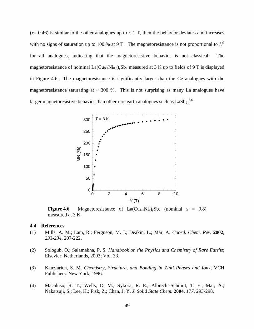
49
(x= 0.46) is similar to the other analogues up to ~ 1 T, then the behavior deviates and increases
with no signs of saturation up to 100 % at 9 T. The magnetoresistance is not proportional to H2
for all analogues, indicating that the magnetoresistive behavior is not classical. The
magnetoresistance of nominal La(Cu0.2Ni0.8)ySb2 measured at 3 K up to fields of 9 T is displayed
in Figure 4.6. The magnetoresistance is significantly larger than the Ce analogues with the
magnetoresistance saturating at ~ 300 %. This is not surprising as many La analogues have
larger magnetoresistive behavior than other rare earth analogues such as LaSb2.5,6
4.4 References
(1) Mills, A. M.; Lam, R.; Ferguson, M. J.; Deakin, L.; Mar, A. Coord. Chem. Rev. 2002,
233-234, 207-222.
(2) Sologub, O.; Salamakha, P. S. Handbook on the Physics and Chemistry of Rare Earths;
Elsevier: Netherlands, 2003; Vol. 33.
(3) Kauzlarich, S. M. Chemistry, Structure, and Bonding in Zintl Phases and Ions; VCH
Publishers: New York, 1996.
(4) Macaluso, R. T.; Wells, D. M.; Sykora, R. E.; Albrecht-Schmitt, T. E.; Mar, A.;
Nakatsuji, S.; Lee, H.; Fisk, Z.; Chan, J. Y. J. Solid State Chem. 2004, 177, 293-298.
0
50
100
150
200
250
300
0 2 4 6 8 10
H (T)
T = 3 K
MR
(%
)
Figure 4.6 Magnetoresistance of La(Cu1-xNix)ySb2 (nominal x = 0.8)
measured at 3 K.

50
(5) Bud'ko, S. L.; Canfield, P. C.; Mielke, C. H.; Lacerda, A. H. Phys. Rev. B 1998, 57,
13624-13638.
(6) Young, D. P.; Goodrich, R. G.; DiTusa, J. F.; Guo, S.; Adams, P. W.; Chan, J. Y.; Hall,
D. Appl. Phys. Lett. 2003, 82, 3713-3715.
(7) Thomas, E. L.; Moldovan, M.; Young, D. P.; Chan, J. Y. Chem. Mater. 2005, 17, 5810-
5816.
(8) Thamizhavel, A.; Takeuchi, T.; Okubo, T.; Yamada, M.; Asai, R.; Kirit, S.; Galatanu, A.;
Yamamoto, E.; Ebihara, T.; Inada, Y.; Settai, R.; Onuki, Y. Phys. Rev. B 2003, 68,
54427.
(9) Siderov, V. A.; Bauer, E. D.; Lee, H.; Nakatsuji, S.; Thompson, J. D.; Fisk, Z. Phys. Rev.
B 2005, 71, 094422-1 - 094422-4.
(10) Muro, Y.; Takeda, N.; Ishikawa, M. J. Alloys Compd. 1997, 257, 23-29.
(11) Lakshmi, K. V.; Menon, L.; Nigam, A. K.; Das, A.; Malik, S. K. Physica B 1996, 223 &
224, 289-291.
(12) Sologub, O.; Hiebl, K.; Rogl, P.; Noël, H.; Bodak, O. J. Alloys Compd. 1994, 210, 153-
157.
(13) Flandorfer, H.; Sologub, O.; Godart, C.; Hiebl, K.; Leith-Jasper, A.; Rogl, P.; Noel, H.
Solid State Commun. 1996, 97, 561-565.
(14) Koyama, T.; Matsumoto, M.; Wada, S.; Muro, Y.; Ishikawa, M. J. Phys. Soc. Jpn. 2001,
70, 3667-3672.
(15) Thamizhavel, A.; Okubo, T.; Yamada, M.; Galatanu, A.; Yamamoto, E.; Inada, Y.;
Ebihara, T.; Onuki, Y. Physica B 2003, 327, 374-377.
(16) Altomare, A.; Burla, M. C.; Camalli, M.; Cascarno, G. L.; Giacovazzo, A.; Guagliardi,
A.; Moliterni, A. G. G.; Polidori, G.; Spagna, R. J. J. Appl. Crystallogr. 1999, 32, 115-
119.
(17) Sheldrick, G. M.; University of Gottingen: Germany, 1997.
(18) Andrukhiv, L. S.; Lysenko, L. O.; Yarmolyuk, Y. P.; Hladyshevsky, E. I. Dopov. Akad.
Nauk Ukr. RSR, Ser. A 1975, 7, 645-648.
(19) Thomas, E. L.; Macaluso, R. T.; Lee, H.; Fisk, Z.; Chan, J. Y. J. Solid State Chem. 2004,
177, 4228-4236.
(20) Wang, R.; Steinfink, H. Inorg. Chem. 1967, 6, 1685-1692.

51
CHAPTER 5 – Rb4M(MoO4)3
5.1 Introduction
The existence of ferroelectricity and magnetism in a single material has generated interest
in recent years because the two phenomena were previously thought to not coexist in the same
material. This new, exciting field has been termed multiferroics and researchers are working to
understand the mechanisms by which these two phenomena can coexist simultaneously. This
research is fueled by the promise of numerous practical applications such as conventional
actuators, transducers, data storage, or memory media.1
One of the more well known mechanisms for ferroelectricity in a perovskite such as
BaTiO3, has the Ti4+
ion shifted towards the corner of the unit cell which creates electric
polarization inducing a charge transfer from filled oxygen 2p orbitals into the empty d-orbitals of
the transition metal.1,2
Empty d-orbitals are necessary for magnetism to exist, so this mechanism
is not conducive to multiferroism. Another mechanism for off-center distortion of the transition
metal site is found in materials with a ns2 lone pair which displaces the parent cation leading to
the loss of inversion symmetry.1 There are both proper and improper inversion symmetry
breaking mechanisms.3 Covalent bonding between 3d
0 transition metal and oxygen seen in
BaTiO3 and 6s2 lone pair polarization seen in compounds such as BiMnO3, BiFeO3, and
Pb(Fe2/3W1/3)O3 are examples of the proper mechanism for losing inversion symmetry.3
Examples of improper loss of inversion symmetry mechanisms include structural transitions as
seen in K2SeO4, Cs2CdI4, and hexagonal RMnO3, charge ordering as seen in LuFe2O4, and
magnetic ordering as seen in RMn2O5, CoCr2O4, and the orthorhombic RMnO3.3 These
mechanisms apply only to ferroelectricity and typically do not allow for the simultaneous
presence of a magnetic moment.

52
Multiferroic materials were in short supply until 2003, when Kimura et al. discovered
that spin frustration causes antiferromagnetic ordering in TbMnO3.4 This rekindled interest in
multiferroic materials and the quest was on to understand and discover more of these intriguing
materials with frustrated spin systems. In 2007, another mechanism came to light in frustrated
magnets where a magnetic spiral structure breaks inversion symmetry and leads to the presence
of electric polarization.3,5
In 2008 CuO, a centrosymmetric material, was identified as an
induced-multiferroic which has a proper-screw magnetic.6 This new mechanism will be useful in
identifying other possible multiferroic materials.
As indicated above, crystal symmetry plays an integral role in predicting and
understanding multiferroic behavior in materials. This is the motivation for the present work.
Full structural determination, understanding temperature induced phase transitions, and the
analyses of disorder in crystals are important in understanding the properties of these materials.
The crystal structural studies of the possible multiferroic double molybdates, Rb4M(MoO4)3, (M
= Mn, Zn, Cu) are reported herein.
5.2 Structural Studies by Single Crystal X-Ray Diffraction
The single crystal X-ray diffraction data of Rb4M(MoO4)3 (M = Mn, Zn, and Cu) were
collected at various temperatures. Due to the extremely hygroscopic nature of the samples, the
crystals were placed in Paratone-N oil to protect the sample from exposure to air and moisture.
A crystal with approximate dimensions of ~ 0.05 x 0.125 x 0.125 mm3 was mounted onto a glass
fiber of the goniometer with epoxy and/or vacuum grease and placed on a Nonius Kappa CCD
X-ray diffractometer (MoKα = 0.71073 Å). Temperature was regulated with a cooled nitrogen
gas stream produced by an Oxford Cryostream Cooler. The unit cell parameters were
determined from images taken at a rotation of 15 °φ. Initial structural models were solved by

53
SIR977 and refined by direct methods using SHELXL97
8. The data were corrected for
absorption and the displacement parameters were refined as anisotropic.
5.2.1 Rb4Mn(MoO4)3
The single crystal X-ray diffraction data was collected at various temperatures for
Rb4Mn(MoO4)3. Data were collected at 298 K, 270 K, and 100 K. The crystal measured had
dimensions of ~ 0.05 x 0.125 x 0.125 mm3. There were two suitable structural models in two
different, hexagonal space group choices: P6 2c (# 190) and P63/mmc (# 194). P6 2c (# 190) is a
non-centrosymmetric space group while P63/mmc (# 194) is a centrosymmetric space group.
The main difference between the two space groups is the presence of three mirrors perpendicular
to the rotation axis in the higher symmetry space group. The systematic absences are the same
for both space groups. Powder patterns were calculated from the single crystal models and both
patterns were identical and matched the experimental powder pattern as shown in Figure 5.1.
Previous structural reports indicate acceptable structural models in three hexagonal space groups:
P63/mmc, P63mc, and P6 2c. However, the centrosymmetric P63/mmc was ruled out due to
Peak from Flux Rb2Mo2O7
Calculated from
Single Crystal
Experimental
3000
2000
1000
0
10 15 20 25 30 35 45 50 55 60 65 70 75 8040
2θ
cp
s
Figure 5.1 Experimental (red) and calculated (black) powder patterns for
Rb4Mn(MoO4)3.
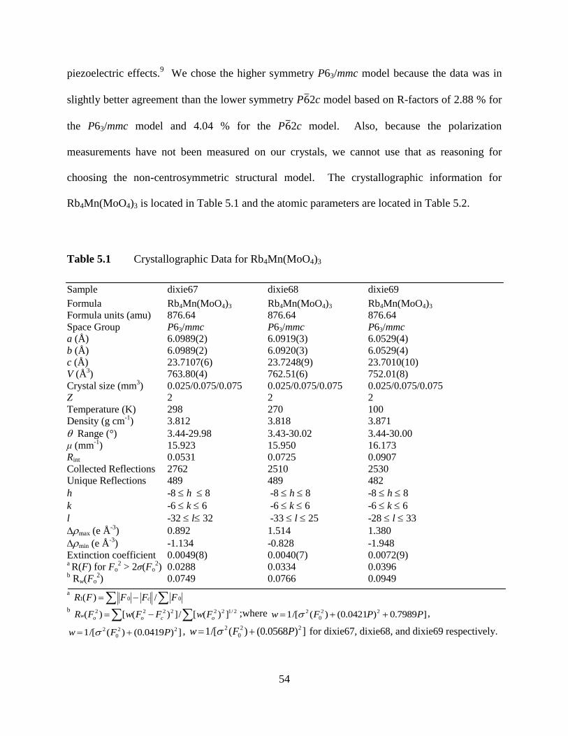
54
piezoelectric effects.9 We chose the higher symmetry P63/mmc model because the data was in
slightly better agreement than the lower symmetry P6 2c model based on R-factors of 2.88 % for
the P63/mmc model and 4.04 % for the P6 2c model. Also, because the polarization
measurements have not been measured on our crystals, we cannot use that as reasoning for
choosing the non-centrosymmetric structural model. The crystallographic information for
Rb4Mn(MoO4)3 is located in Table 5.1 and the atomic parameters are located in Table 5.2.
Table 5.1 Crystallographic Data for Rb4Mn(MoO4)3
Sample dixie67 dixie68 dixie69
Formula Rb4Mn(MoO4)3 Rb4Mn(MoO4)3 Rb4Mn(MoO4)3
Formula units (amu) 876.64 876.64 876.64
Space Group P63/mmc P63/mmc P63/mmc
a (Å) 6.0989(2) 6.0919(3) 6.0529(4)
b (Å) 6.0989(2) 6.0920(3) 6.0529(4)
c (Å) 23.7107(6) 23.7248(9) 23.7010(10)
V (Å3) 763.80(4) 762.51(6) 752.01(8)
Crystal size (mm3) 0.025/0.075/0.075 0.025/0.075/0.075 0.025/0.075/0.075
Z 2 2 2
Temperature (K) 298 270 100
Density (g cm-1
) 3.812 3.818 3.871
Range (°) 3.44-29.98 3.43-30.02 3.44-30.00
μ (mm-1
) 15.923 15.950 16.173
Rint 0.0531 0.0725 0.0907
Collected Reflections 2762 2510 2530
Unique Reflections 489 489 482
h -8 h 8 -8 h 8 -8 h 8
k -6 k 6 -6 k 6 -6 k 6
l -32 l 32 -33 l 25 -28 l 33
max (e Å-3
) 0.892 1.514 1.380
min (e Å-3
) -1.134 -0.828 -1.948
Extinction coefficient 0.0049(8) 0.0040(7) 0.0072(9) a R(F) for Fo
2 > 2σ(Fo
2) 0.0288 0.0334 0.0396
b Rw(Fo
2) 0.0749 0.0766 0.0949
a 001 /)( FFFFR c
b 2/1222222 ])([/])([)( ocoow FwFFwFR ;where ]0.7989)0.0421()(/[1 22
0
2 PPFw ,
])0.0419()(/[1 22
0
2 PFw , ])0.0568()(/[1 22
0
2 PFw for dixie67, dixie68, and dixie69 respectively.

55
Table 5.2 Atomic Positions and Displacement Parameters for Rb4Mn(MoO4)3
Atom Wyckoff site x y z Ueq (Å
2)
a Occupancy
dixie67 – 298 K
Rb1 4f ⅓ ⅔ 0.15755(3) 0.0344(3) 1
Rb2 4f ⅔ ⅓ 0.02849(3) 0.0283(3) 1
Mn1 2a 0 0 ¼ 0.0281(4) 1
Mo1 4e 0 0 0.09016(2) 0.0196(2) 1
Mo2 4f ⅔ ⅓ 0.22782(6) 0.0255(5) 0.48
O1 4e 0 0 0.1645(2) 0.056(2) 1
O2 12k 0.1555(3) 0.3109(6) 0.06565(15) 0.0406(9) 1
O3 4f ⅔ ⅓ 0.1557(4) 0.047(6) 0.50
O4 12j 0.3859(12) 0.3283(13) ¼ 0.041(2) 0.51
dixie68 – 270 K
Rb1 4f ⅓ ⅔ 0.15755(3) 0.0306(3) 1
Rb2 4f ⅔ ⅓ 0.02850(4) 0.0244(3) 1
Mn1 2a 0 0 ¼ 0.0240(5) 1
Mo1 4e 0 0 0.09006(3) 0.0167(2) 1
Mo2 4f ⅔ ⅓ 0.22787(7) 0.0216(6) 0.48
O1 4e 0 0 0.1647(2) 0.053(2) 1
O2 12k 0.1556(3) 0.3112(7) 0.06566(16) 0.0352(10) 1
O3 4f ⅔ ⅓ 0.1556(4) 0.037(6) 0.50
O4 12j 0.3840(13) 0.3286(14) ¼ 0.037(3) 0.52
dixie69 – 100 K
Rb1 4f ⅓ ⅔ 0.15728(4) 0.0176(4) 1
Rb2 4f ⅔ ⅓ 0.02879(4) 0.0143(4) 1
Mn1 2a 0 0 ¼ 0.0164(6) 1
Mo1 4e 0 0 0.08945(3) 0.0113(3) 1
Mo2 4f ⅔ ⅓ 0.22778(9) 0.0160(8) 0.48
O1 4e 0 0 0.1649(3) 0.033(3) 1
O2 12k 0.1568(5) 0.3136(10) 0.0649(2) 0.0233(13) 1
O3 4f ⅔ ⅓ 0.1551(6) 0.016(6) 0.46
O4 12j 0.385(2) 0.332(2) ¼ 0.028(3) 0.50 aUeq is defined as one-third of the trace of the orthogonalized Uij tensor.
Figure 5.2 displays the structure of Rb4Mn(MoO4)3 as well as the coordination around the
Mn1 atom. The structure consists of MnO5 trigonal bipyramids surrounded by five Mo
tetrahedra: two Mo2 tetrahedra in the capping positions and three Mo1 tetrahedra in the basal
plane. Rb4Mn(MoO4)3 is isostructural to Cs4Cu(MoO4)3.9 There are several atoms in this
structure that are disordered. The three O4 atoms in the basal plane of the Mn trigonal bipyramid
and each Mo2, O3, and O4 atoms that comprise the Mo2 tetrahedra are disordered. This disorder
is displayed by ½ occupied sites in the atomic positions. The Mo2 tetrahedra seem to be inverted
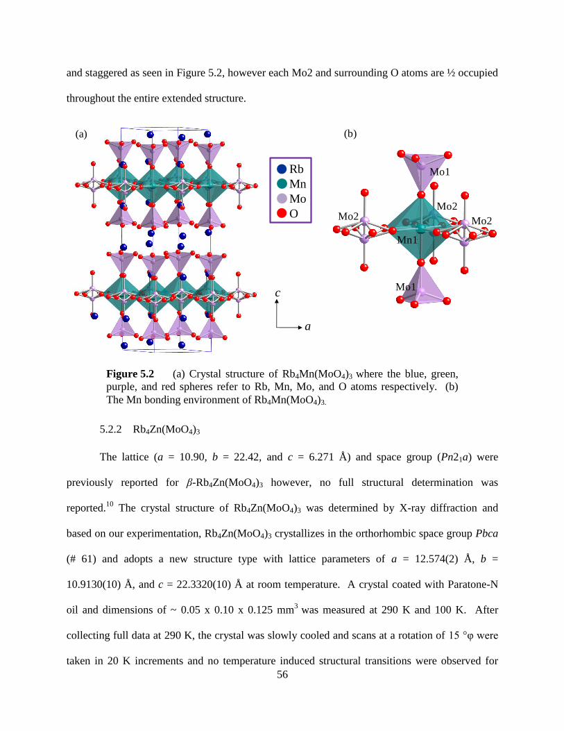
56
and staggered as seen in Figure 5.2, however each Mo2 and surrounding O atoms are ½ occupied
throughout the entire extended structure.
5.2.2 Rb4Zn(MoO4)3
The lattice (a = 10.90, b = 22.42, and c = 6.271 Å) and space group (Pn21a) were
previously reported for β-Rb4Zn(MoO4)3 however, no full structural determination was
reported.10
The crystal structure of Rb4Zn(MoO4)3 was determined by X-ray diffraction and
based on our experimentation, Rb4Zn(MoO4)3 crystallizes in the orthorhombic space group Pbca
(# 61) and adopts a new structure type with lattice parameters of a = 12.574(2) Å, b =
10.9130(10) Å, and c = 22.3320(10) Å at room temperature. A crystal coated with Paratone-N
oil and dimensions of ~ 0.05 x 0.10 x 0.125 mm3
was measured at 290 K and 100 K. After
collecting full data at 290 K, the crystal was slowly cooled and scans at a rotation of 15 °φ were
taken in 20 K increments and no temperature induced structural transitions were observed for
Mo1
Mo2
Mn1
Rb
Mn
Mo
O
a
cMo1
Mo2
Mo2
(a) (b)
Figure 5.2 (a) Crystal structure of Rb4Mn(MoO4)3 where the blue, green,
purple, and red spheres refer to Rb, Mn, Mo, and O atoms respectively. (b)
The Mn bonding environment of Rb4Mn(MoO4)3.

57
Rb4Zn(MoO4)3. Crystallographic information for Rb4Zn(MoO4)3 is located in Table 5.3 and the
atomic parameters are located in Table 5.4.
Table 5.3 Crystallographic Data for Rb4Zn(MoO4)3
Sample dixie75 dixie76
Formula Rb4Zn(MoO4)3 Rb4Zn(MoO4)3
Formula units (amu) 887.07 887.07
Space Group Pbca Pbca
a (Å) 12.574(2) 12.485(2)
b (Å) 10.9130(10) 10.8750(10)
c (Å) 22.3320(10) 22.2660(10)
V (Å3) 3064.4(6) 3023.2(6)
Crystal size (mm3) 0.05/0.10/0.125 0.05/0.10/0.125
Z 8 8
Temperature (K) 290 100
Density (g cm-1
) 3.845 3.898
Range (°) 2.44-30.04 2.45-30.02
μ (mm-1
) 16.617 16.843
Rint 0.0703 0.0535
Collected Reflections 8345 8235
Unique Reflections 2478 2922
h -17 h 17 -17 h 17
k -15 k 15 -15 k 15
l -31 l 31 -31 l 31
max (e Å-3
) 4.515 2.495
min (e Å-3
) -2.607 -1.940
Extinction coefficient 0.00052(4) 0.000134(18) a R(F) for Fo
2 > 2σ(Fo
2) 0.0537 0.0456
b Rw(Fo
2) 0.1132 0.0919
a 001 /)( FFFFR c
b 2/1222222 ])([/])([)( ocoow FwFFwFR ;where 2 2 2
01/ [ ( ) (0.0579 ) ]w F P ,
2 2 2
01/ [ ( ) (0.0394 ) 9.0735 ]w F P P for dixie75 and dixie76 respectively.
Table 5.4 Atomic Positions and Displacement Parameters for Rb4Zn(MoO4)3
Atom Wyckoff site x y z Ueq (Å
2)
a
dixie75 – 290 K
Rb1 8c 0.62666(7) 0.91895(7) 0.97177(4) 0.0217(2)
Rb2 8c 0.87590(7) 0.08521(7) 0.03049(4) 0.0277(2)
Rb3 8c 0.10741(7) 0.57137(8) 0.83923(3) 0.0281(2)
Rb4 8c 0.62284(7) 0.59654(8) 0.84237(3) 0.0297(2)
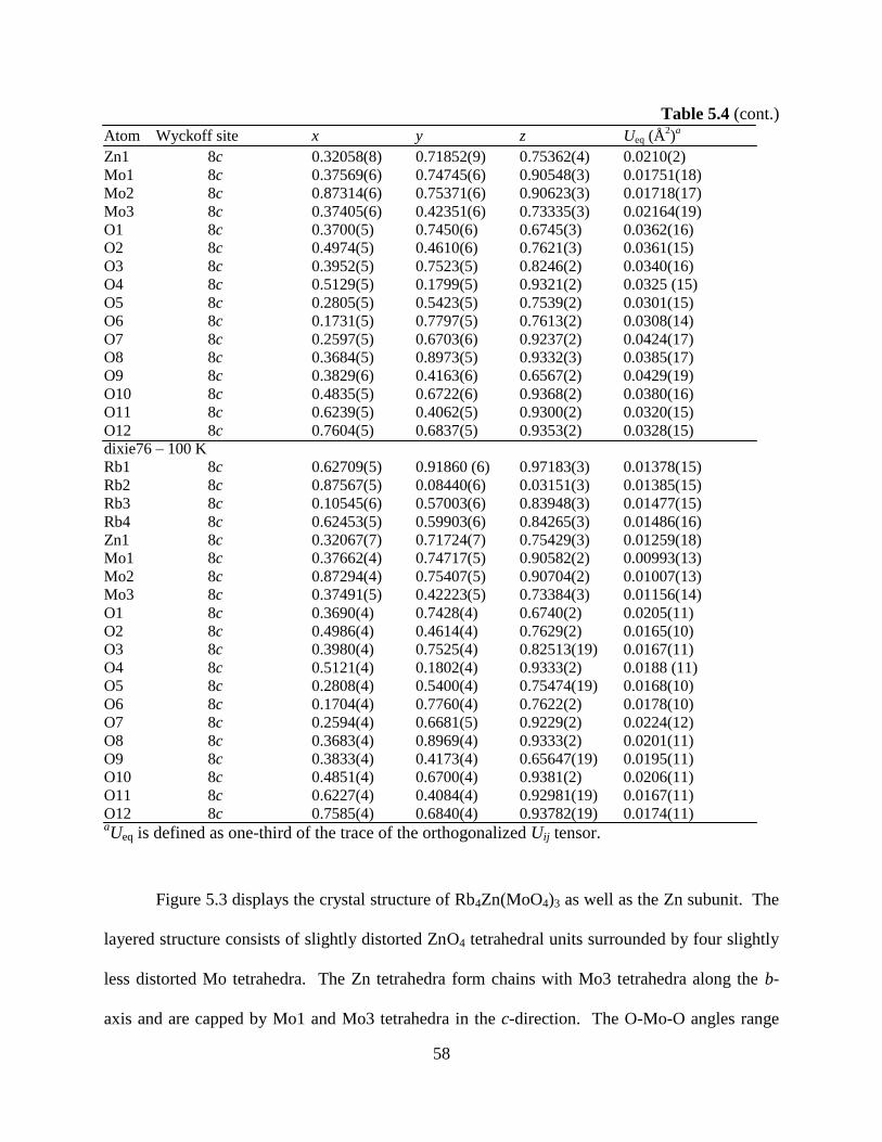
58
Table 5.4 (cont.)
Atom Wyckoff site x y z Ueq (Å2)
a
Zn1 8c 0.32058(8) 0.71852(9) 0.75362(4) 0.0210(2)
Mo1 8c 0.37569(6) 0.74745(6) 0.90548(3) 0.01751(18)
Mo2 8c 0.87314(6) 0.75371(6) 0.90623(3) 0.01718(17)
Mo3 8c 0.37405(6) 0.42351(6) 0.73335(3) 0.02164(19)
O1 8c 0.3700(5) 0.7450(6) 0.6745(3) 0.0362(16)
O2 8c 0.4974(5) 0.4610(6) 0.7621(3) 0.0361(15)
O3 8c 0.3952(5) 0.7523(5) 0.8246(2) 0.0340(16)
O4 8c 0.5129(5) 0.1799(5) 0.9321(2) 0.0325 (15)
O5 8c 0.2805(5) 0.5423(5) 0.7539(2) 0.0301(15)
O6 8c 0.1731(5) 0.7797(5) 0.7613(2) 0.0308(14)
O7 8c 0.2597(5) 0.6703(6) 0.9237(2) 0.0424(17)
O8 8c 0.3684(5) 0.8973(5) 0.9332(3) 0.0385(17)
O9 8c 0.3829(6) 0.4163(6) 0.6567(2) 0.0429(19)
O10 8c 0.4835(5) 0.6722(6) 0.9368(2) 0.0380(16)
O11 8c 0.6239(5) 0.4062(5) 0.9300(2) 0.0320(15)
O12 8c 0.7604(5) 0.6837(5) 0.9353(2) 0.0328(15)
dixie76 – 100 K
Rb1 8c 0.62709(5) 0.91860 (6) 0.97183(3) 0.01378(15)
Rb2 8c 0.87567(5) 0.08440(6) 0.03151(3) 0.01385(15)
Rb3 8c 0.10545(6) 0.57003(6) 0.83948(3) 0.01477(15)
Rb4 8c 0.62453(5) 0.59903(6) 0.84265(3) 0.01486(16)
Zn1 8c 0.32067(7) 0.71724(7) 0.75429(3) 0.01259(18)
Mo1 8c 0.37662(4) 0.74717(5) 0.90582(2) 0.00993(13)
Mo2 8c 0.87294(4) 0.75407(5) 0.90704(2) 0.01007(13)
Mo3 8c 0.37491(5) 0.42223(5) 0.73384(3) 0.01156(14)
O1 8c 0.3690(4) 0.7428(4) 0.6740(2) 0.0205(11)
O2 8c 0.4986(4) 0.4614(4) 0.7629(2) 0.0165(10)
O3 8c 0.3980(4) 0.7525(4) 0.82513(19) 0.0167(11)
O4 8c 0.5121(4) 0.1802(4) 0.9333(2) 0.0188 (11)
O5 8c 0.2808(4) 0.5400(4) 0.75474(19) 0.0168(10)
O6 8c 0.1704(4) 0.7760(4) 0.7622(2) 0.0178(10)
O7 8c 0.2594(4) 0.6681(5) 0.9229(2) 0.0224(12)
O8 8c 0.3683(4) 0.8969(4) 0.9333(2) 0.0201(11)
O9 8c 0.3833(4) 0.4173(4) 0.65647(19) 0.0195(11)
O10 8c 0.4851(4) 0.6700(4) 0.9381(2) 0.0206(11)
O11 8c 0.6227(4) 0.4084(4) 0.92981(19) 0.0167(11)
O12 8c 0.7585(4) 0.6840(4) 0.93782(19) 0.0174(11) aUeq is defined as one-third of the trace of the orthogonalized Uij tensor.
Figure 5.3 displays the crystal structure of Rb4Zn(MoO4)3 as well as the Zn subunit. The
layered structure consists of slightly distorted ZnO4 tetrahedral units surrounded by four slightly
less distorted Mo tetrahedra. The Zn tetrahedra form chains with Mo3 tetrahedra along the b-
axis and are capped by Mo1 and Mo3 tetrahedra in the c-direction. The O-Mo-O angles range

59
from 107.9 ° - 111.1 ° for Mo1, 108.8 ° - 110.1 ° for Mo2, and 108.7 ° - 112.1 ° for Mo3
indicating a slight deviation from the expected angle of 109.5 °. The O-Zn-O angles range from
103.5 ° - 126.4 ° for the ZnO4 tetrahedra indicating more distortion than the MoO4 units.
Selected interatomic distances and bond angles are located in Table 5.5. The distances are
consistent with the ionic radii of Rb1+
, Zn2+
, and Mo6+
.11
The notable difference between this
structure and the Rb4Mn(MoO4)3 structure is the lack of disorder and the bonding environment of
the transition metal. The Mn analogue consists of a Mn trigonal bipyramid while the Zn
analogue contains slightly distorted Zn tetrahedra.
Table 5.5 Selected Interatomic Distances (Å) for Rb4Zn(MoO4)3
Mo1 – O7 1.740(5) Rb1 – O9 2.860(4) Rb2 – O10 2.866(5)
Mo1 – O8 1.742(5) Rb1 – O8 2.915(5) Rb2 – O12 2.886(5)
Mo1 – O10 1.748(5) Rb1 – O4 2.939(5) Rb2 – O11 2.965(4)
Mo1 – O3 1.817(4) Rb1 – O7 3.018(5) Rb2 – O8 3.152(5)
c
b
Mo1
Mo2
Mo3 Mo3
Zn1Rb
Zn
Mo
O
(a) (b)
Figure 5.3 (a) Crystal structure of Rb4Zn(MoO4)3 as viewed down the a
axis where the blue, green, purple, and red spheres refer to Rb, Zn, Mo, and O
atoms respectively. (b) Zn bonding environment of Rb4Zn(MoO4)3.

60
Table 5.5 (cont.) Rb1 – O12 3.126(5) Rb2 – O10 3.159(5)
Mo2 – O4 1.746(5) Rb1 – O11 3.263(5) Rb2 – O4 3.173(5)
Mo2 – O11 1.754(4) Rb1 – O4 3.300(5) Rb2 – O11 3.203(5)
Mo2 – O12 1.758(5) Rb1 – O12 3.309(5) Rb2 – O7 3.268(5)
Mo2 – O1 1.808(5) Rb1 – O10 3.319(5) Rb2 – O7 3.334(5)
Rb1 – O8 3.352(5)
Mo3 – O9 1.727(4) Rb4 – O2 2.805(4)
Mo3 – O2 1.727(5) Rb3 – O4 2.820(5) Rb4 – O11 2.840(4)
Mo3 – O5 1.800(5) Rb3 – O8 2.830(5) Rb4 – O10 2.853(5)
Mo3 – O6 1.802(5) Rb3 – O7 2.878(5) Rb4 – O12 2.853(5)
Rb3 – O2 2.893(5) Rb4 – O5 2.986(5)
Zn1 – O3 1.889(5) Rb3 – O5 2.908(5) Rb4 – O6 3.079(5)
Zn1 – O1 1.908(5) Rb3 – O6 2.939(4) Rb4 – O3 3.307(5)
Zn1 – O6 1.990(5) Rb3 – O9 3.234(5)
Zn1 – O5 1.991(5)
5.2.3 Rb4Cu(MoO4)3
Rb4Cu(MoO4)3 undergoes two temperature dependent phase transitions.12
Above room
temperature the structure adopts a hexagonal structure, at room temperature the crystal adopts an
orthorhombic structure, and around 103 K the crystal is reported to adopt a monoclinic
structure.12
Based on current experiments at 298 K, the compound adopts an orthorhombic
structure (Pnma #62) with a lattice of a = 10.581(2) Å, b = 23.213(4) Å, and c = 6.078(1) Å.
One sample batch yielded a crystal that adopted the hexagonal structure (6.1 x 23.2 Å), however
this result was not found in other batches of Rb4Cu(MoO4)3 crystals. The crystallographic
information for both the hexagonal and orthorhombic phases of Rb4Cu(MoO4)3 are located in
Table 5.6 and the atomic coordinates and displacement parameters are located in Table 5.7. A
similar orthorhombic lattice was also reported for β-Rb4Zn(MoO4)3 which adopts the Pn21a
space group, however no other structural information was reported for this compound.10
The
lattice is similar to the orthorhombic compound K4Zn(MoO4)3 which crystallizes in the space
group P212121.13,14
The space groups P212121 and Pnma belong to the same sub group and both
have 21 screw axes in all three directions, while Pnma also has a mirror, glide planes, and an
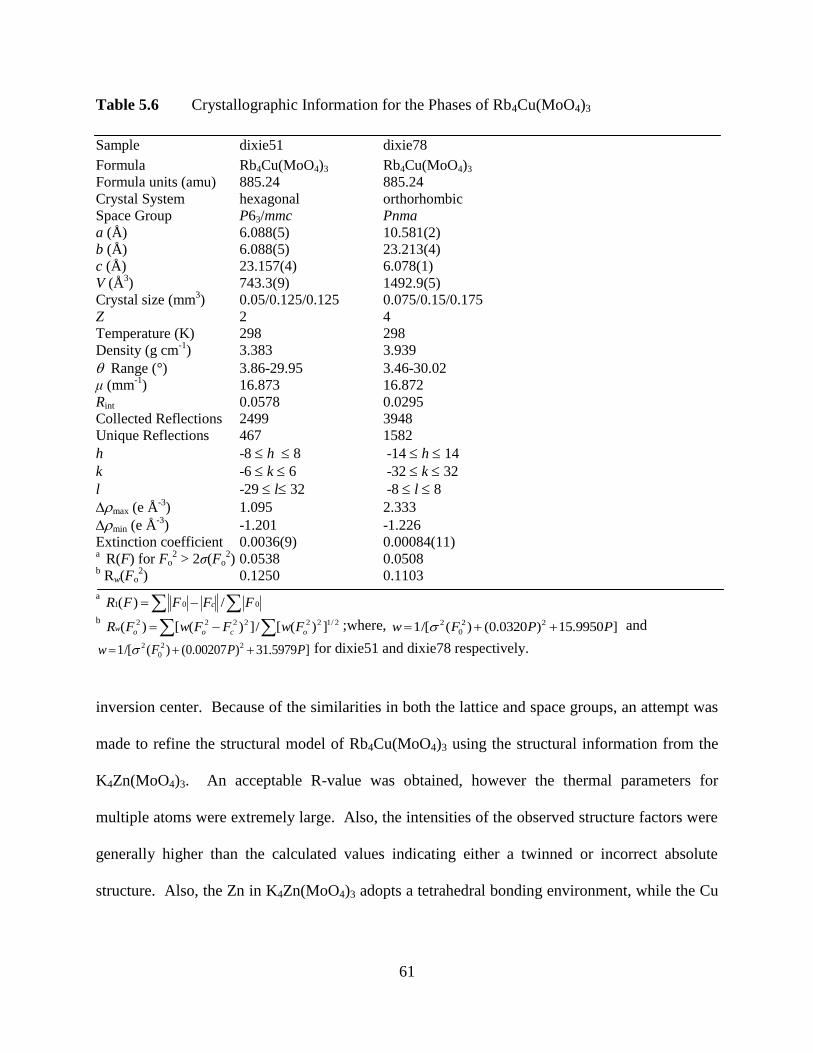
61
Table 5.6 Crystallographic Information for the Phases of Rb4Cu(MoO4)3
Sample dixie51 dixie78
Formula Rb4Cu(MoO4)3 Rb4Cu(MoO4)3
Formula units (amu) 885.24 885.24
Crystal System hexagonal orthorhombic
Space Group P63/mmc Pnma
a (Å) 6.088(5) 10.581(2)
b (Å) 6.088(5) 23.213(4)
c (Å) 23.157(4) 6.078(1)
V (Å3) 743.3(9) 1492.9(5)
Crystal size (mm3) 0.05/0.125/0.125 0.075/0.15/0.175
Z 2 4
Temperature (K) 298 298
Density (g cm-1
) 3.383 3.939
Range (°) 3.86-29.95 3.46-30.02
μ (mm-1
) 16.873 16.872
Rint 0.0578 0.0295
Collected Reflections 2499 3948
Unique Reflections 467 1582
h -8 h 8 -14 h 14
k -6 k 6 -32 k 32
l -29 l 32 -8 l 8
max (e Å-3
) 1.095 2.333
min (e Å-3
) -1.201 -1.226
Extinction coefficient 0.0036(9) 0.00084(11) a R(F) for Fo
2 > 2σ(Fo
2) 0.0538 0.0508
b Rw(Fo
2) 0.1250 0.1103
a 001 /)( FFFFR c
b 2/1222222 ])([/])([)( ocoow FwFFwFR ;where, ]15.9950)0.0320()(/[1 22
0
2 PPFw and
]31.5979)0.00207()(/[1 22
0
2 PPFw for dixie51 and dixie78 respectively.
inversion center. Because of the similarities in both the lattice and space groups, an attempt was
made to refine the structural model of Rb4Cu(MoO4)3 using the structural information from the
K4Zn(MoO4)3. An acceptable R-value was obtained, however the thermal parameters for
multiple atoms were extremely large. Also, the intensities of the observed structure factors were
generally higher than the calculated values indicating either a twinned or incorrect absolute
structure. Also, the Zn in K4Zn(MoO4)3 adopts a tetrahedral bonding environment, while the Cu
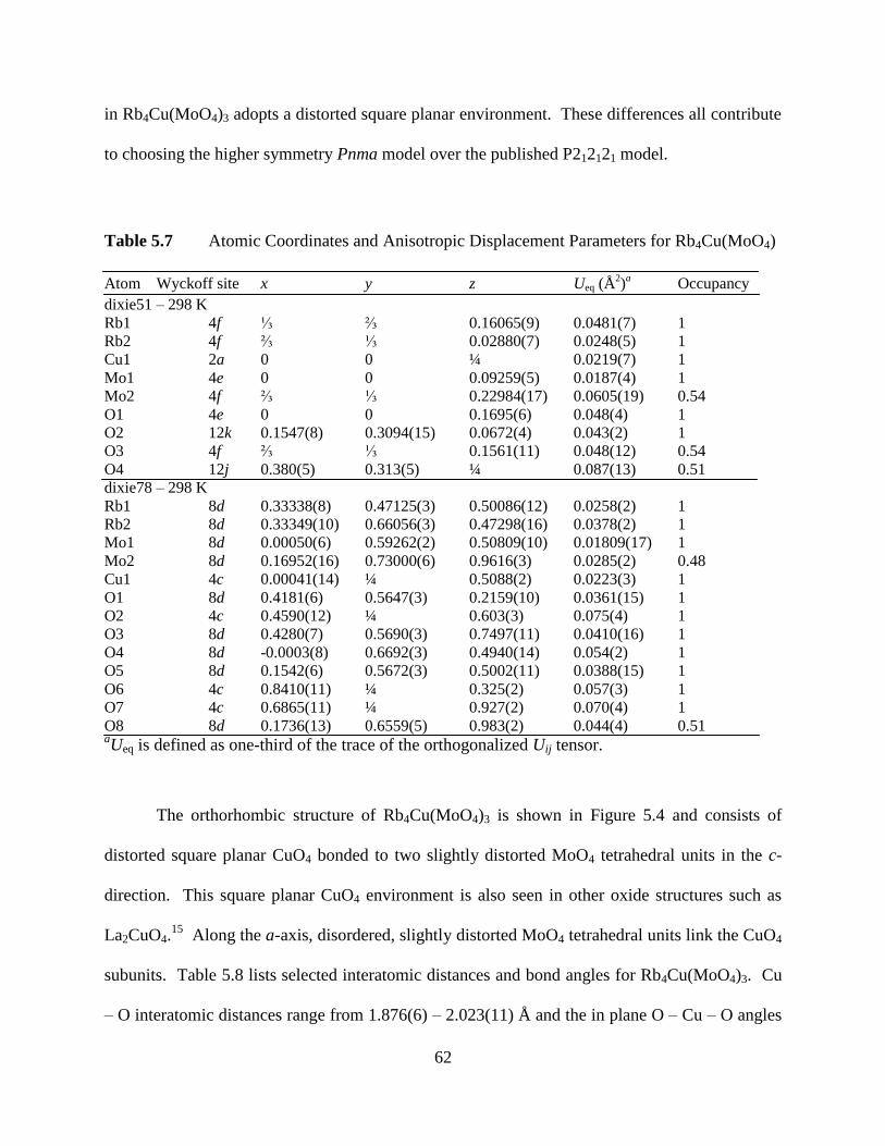
62
in Rb4Cu(MoO4)3 adopts a distorted square planar environment. These differences all contribute
to choosing the higher symmetry Pnma model over the published P212121 model.
Table 5.7 Atomic Coordinates and Anisotropic Displacement Parameters for Rb4Cu(MoO4)
Atom Wyckoff site x y z Ueq (Å2)
a Occupancy
dixie51 – 298 K
Rb1 4f ⅓ ⅔ 0.16065(9) 0.0481(7) 1
Rb2 4f ⅔ ⅓ 0.02880(7) 0.0248(5) 1
Cu1 2a 0 0 ¼ 0.0219(7) 1
Mo1 4e 0 0 0.09259(5) 0.0187(4) 1
Mo2 4f ⅔ ⅓ 0.22984(17) 0.0605(19) 0.54
O1 4e 0 0 0.1695(6) 0.048(4) 1
O2 12k 0.1547(8) 0.3094(15) 0.0672(4) 0.043(2) 1
O3 4f ⅔ ⅓ 0.1561(11) 0.048(12) 0.54
O4 12j 0.380(5) 0.313(5) ¼ 0.087(13) 0.51
dixie78 – 298 K
Rb1 8d 0.33338(8) 0.47125(3) 0.50086(12) 0.0258(2) 1
Rb2 8d 0.33349(10) 0.66056(3) 0.47298(16) 0.0378(2) 1
Mo1 8d 0.00050(6) 0.59262(2) 0.50809(10) 0.01809(17) 1
Mo2 8d 0.16952(16) 0.73000(6) 0.9616(3) 0.0285(2) 0.48
Cu1 4c 0.00041(14) ¼ 0.5088(2) 0.0223(3) 1
O1 8d 0.4181(6) 0.5647(3) 0.2159(10) 0.0361(15) 1
O2 4c 0.4590(12) ¼ 0.603(3) 0.075(4) 1
O3 8d 0.4280(7) 0.5690(3) 0.7497(11) 0.0410(16) 1
O4 8d -0.0003(8) 0.6692(3) 0.4940(14) 0.054(2) 1
O5 8d 0.1542(6) 0.5672(3) 0.5002(11) 0.0388(15) 1
O6 4c 0.8410(11) ¼ 0.325(2) 0.057(3) 1
O7 4c 0.6865(11) ¼ 0.927(2) 0.070(4) 1
O8 8d 0.1736(13) 0.6559(5) 0.983(2) 0.044(4) 0.51 aUeq is defined as one-third of the trace of the orthogonalized Uij tensor.
The orthorhombic structure of Rb4Cu(MoO4)3 is shown in Figure 5.4 and consists of
distorted square planar CuO4 bonded to two slightly distorted MoO4 tetrahedral units in the c-
direction. This square planar CuO4 environment is also seen in other oxide structures such as
La2CuO4.15
Along the a-axis, disordered, slightly distorted MoO4 tetrahedral units link the CuO4
subunits. Table 5.8 lists selected interatomic distances and bond angles for Rb4Cu(MoO4)3. Cu
– O interatomic distances range from 1.876(6) – 2.023(11) Å and the in plane O – Cu – O angles
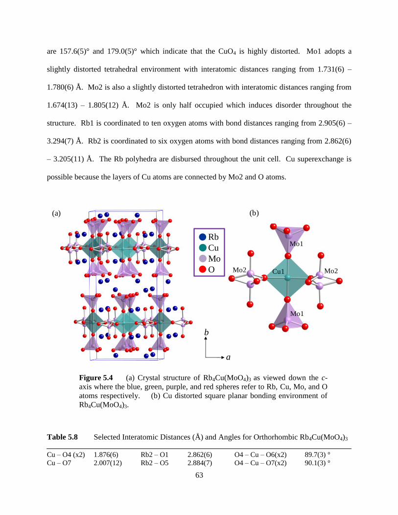
63
are 157.6(5)° and 179.0(5)° which indicate that the CuO4 is highly distorted. Mo1 adopts a
slightly distorted tetrahedral environment with interatomic distances ranging from 1.731(6) –
1.780(6) Å. Mo2 is also a slightly distorted tetrahedron with interatomic distances ranging from
1.674(13) – 1.805(12) Å. Mo2 is only half occupied which induces disorder throughout the
structure. Rb1 is coordinated to ten oxygen atoms with bond distances ranging from 2.905(6) –
3.294(7) Å. Rb2 is coordinated to six oxygen atoms with bond distances ranging from 2.862(6)
– 3.205(11) Å. The Rb polyhedra are disbursed throughout the unit cell. Cu superexchange is
possible because the layers of Cu atoms are connected by Mo2 and O atoms.
Table 5.8 Selected Interatomic Distances (Å) and Angles for Orthorhombic Rb4Cu(MoO4)3
Cu – O4 (x2) 1.876(6) Rb2 – O1 2.862(6) O4 – Cu – O6(x2) 89.7(3) °
Cu – O7 2.007(12) Rb2 – O5 2.884(7) O4 – Cu – O7(x2) 90.1(3) °
Figure 5.4 (a) Crystal structure of Rb4Cu(MoO4)3 as viewed down the c-
axis where the blue, green, purple, and red spheres refer to Rb, Cu, Mo, and O
atoms respectively. (b) Cu distorted square planar bonding environment of
Rb4Cu(MoO4)3.
a
b
Cu1
Mo1
Mo2 Mo2
Mo1
Rb
Cu
Mo
O
(a) (b)
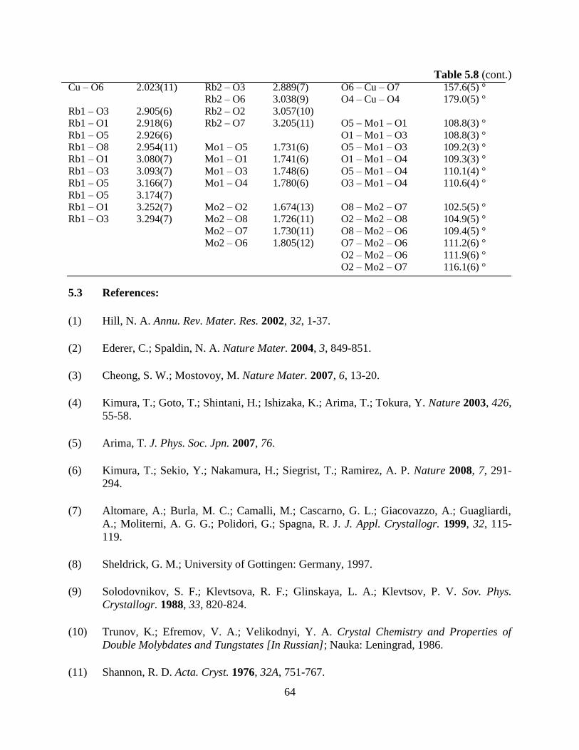
64
Table 5.8 (cont.) Cu – O6 2.023(11) Rb2 – O3 2.889(7) O6 – Cu – O7 157.6(5) °
Rb2 – O6 3.038(9) O4 – Cu – O4 179.0(5) °
Rb1 – O3 2.905(6) Rb2 – O2 3.057(10)
Rb1 – O1 2.918(6) Rb2 – O7 3.205(11) O5 – Mo1 – O1 108.8(3) °
Rb1 – O5 2.926(6) O1 – Mo1 – O3 108.8(3) °
Rb1 – O8 2.954(11) Mo1 – O5 1.731(6) O5 – Mo1 – O3 109.2(3) °
Rb1 – O1 3.080(7) Mo1 – O1 1.741(6) O1 – Mo1 – O4 109.3(3) °
Rb1 – O3 3.093(7) Mo1 – O3 1.748(6) O5 – Mo1 – O4 110.1(4) °
Rb1 – O5 3.166(7) Mo1 – O4 1.780(6) O3 – Mo1 – O4 110.6(4) °
Rb1 – O5 3.174(7)
Rb1 – O1 3.252(7) Mo2 – O2 1.674(13) O8 – Mo2 – O7 102.5(5) °
Rb1 – O3 3.294(7) Mo2 – O8 1.726(11) O2 – Mo2 – O8 104.9(5) °
Mo2 – O7 1.730(11) O8 – Mo2 – O6 109.4(5) °
Mo2 – O6 1.805(12) O7 – Mo2 – O6 111.2(6) °
O2 – Mo2 – O6 111.9(6) °
O2 – Mo2 – O7 116.1(6) °
5.3 References:
(1) Hill, N. A. Annu. Rev. Mater. Res. 2002, 32, 1-37.
(2) Ederer, C.; Spaldin, N. A. Nature Mater. 2004, 3, 849-851.
(3) Cheong, S. W.; Mostovoy, M. Nature Mater. 2007, 6, 13-20.
(4) Kimura, T.; Goto, T.; Shintani, H.; Ishizaka, K.; Arima, T.; Tokura, Y. Nature 2003, 426,
55-58.
(5) Arima, T. J. Phys. Soc. Jpn. 2007, 76.
(6) Kimura, T.; Sekio, Y.; Nakamura, H.; Siegrist, T.; Ramirez, A. P. Nature 2008, 7, 291-
294.
(7) Altomare, A.; Burla, M. C.; Camalli, M.; Cascarno, G. L.; Giacovazzo, A.; Guagliardi,
A.; Moliterni, A. G. G.; Polidori, G.; Spagna, R. J. J. Appl. Crystallogr. 1999, 32, 115-
119.
(8) Sheldrick, G. M.; University of Gottingen: Germany, 1997.
(9) Solodovnikov, S. F.; Klevtsova, R. F.; Glinskaya, L. A.; Klevtsov, P. V. Sov. Phys.
Crystallogr. 1988, 33, 820-824.
(10) Trunov, K.; Efremov, V. A.; Velikodnyi, Y. A. Crystal Chemistry and Properties of
Double Molybdates and Tungstates [In Russian]; Nauka: Leningrad, 1986.
(11) Shannon, R. D. Acta. Cryst. 1976, 32A, 751-767.

65
(12) Klevtsov, P. V.; Kim, V. G.; Kruglik, A. I.; Klevtsova, R. F. Sov. Phys. Crystallogr.
1989, 34, 384-386.
(13) Gicquel-Mayer, C.; Mayer, M. M.; Perez, G. Chimie Minerale 1976, 283, 533-535.
(14) Gicquel-Mayer, C.; Mayer, M.; Perez, G. Rev. Chem. Min. 1980, 17, 445-457.
(15) Chaillout, C.; Cheong, S. W.; Fisk, Z.; Lehmann, M. S.; Marezio, M.; Morosin, B.;
Schirber, J. E. Physica Scripta. 1989, T29, 97-99.

66
CHAPTER 6 – CONCLUSION
One of the primary goals of this dissertation was to gain a better understanding of
structural effects on the physical properties of highly correlated compounds. Identifying
structural features in extended solids that favor a desired behavior will help with the design of
future materials. More correlations of structure and properties are needed to understand the
complex physical properties and to predict the properties of new materials. By growing high-
quality single crystals of compounds, detailed structural analyses and physical property
measurements can be done. For example, it is well known that layered compounds typically
display magnetic anisotropy. It would be beneficial to be able to identify a certain structural
features that could lead to desired or unconventional behavior. The key is simply knowing
where to look.
The dominant theme of this dissertation revolves around layered antimonide compounds
which typically possess unique structural features, unusual bonding, and interesting physical
properties. Antimony resides along the metal – insulating border making this phase space
attractive to investigate. A systematic study of the orthorhombic CeNiSb3 structure type was
conducted in an attempt to correlate structure and properties. By using Sn to grow larger single
crystals of CeNiSb3, a new pseudo-ternary compound, LnNi(Sn,Sb)3, was discovered. The
substitution of the magnetic rare earth element allows for the study of structural changes as well
as physical property effects. Another study was done by the substitution of the transition metal
Ni with Co or Cu of LnNiSb2 i.e. what happens to the structure and physics when changing
carrier density. It was discovered that Cu’s coordination preferentially occupies the tetrahedral
environment seen in the tetragonal CeCuSb2 structure.
Another important part of this work is the structural study of the double molybdates
Rb4M(MoO4)3 (M = Mn, Zn, Cu) compounds. These materials were chosen for investigation

67
because they have frustrated triangular lattices which may lead to polarization. Also the Cu
analogue is expected to be a S = ½ system which exhibits both frustration and quantum
fluctuation. Research of multiferroic materials is extremely attractive because of the promise of
new practical applications. Crystal symmetry plays an integral role in predicting and
understanding multiferroic behavior in materials. Rb4M(MoO4)3 (M = Mn, Zn, Cu) compounds
have promising magnetic and electrical behaviors. The Zn and Cu analogues adopt different,
orthorhombic structures which are both new structure types. The detailed structural study
provided here will be vital in understanding and formulating a mechanism for any multiferroic
behavior.
The appendices which follow this chapter provide information on collaborative projects.
Structural details of compounds such as LnPdSb3, EuCu9Sn4, VB2, and Y2-xCexTi2O7 are
discussed within. These projects also follow the structure-property correlation theme that is seen
throughout this dissertation.
68
APPENDIX 1 – STRUCTURE DETERMINATION OF LnPdSb3 (Ln = La, Ce)
A1.1 Introduction
There are seven ternary compounds in the Ce–Pd–Sb system that have been reported thus
far: CePdSb,2 CePd2Sb2,
3 CePdSb3,
4 CePdSb2,
5 Ce3Pd6Sb5,
6 Ce8Pd24Sb,
7 and Ce2Pd9Sb3.
8 Some
of these phases show heavy fermion behavior. Heavy fermions possess conduction electrons that
have larger effective masses one-hundred times the mass of a free-electron.9 This leads to a
Sommerfeld coefficient (γ) greater than 100 mJ mol-1
K-2
. The Sommerfeld coefficient is
obtained through a fit from heat capacity measurements after subtracting from the phonon
contribution. Ce8Pd24Sb, has a of ~400 mJ mol-1
K-2
, 10
while CePdSb2 possesses a relatively
large enhanced mass with of ~100 mJ mol-1
K-2
. 11
CePdSb3, of the CaBe2Ge2 structure type,12
shows no evidence of magnetic ordering and has a of ~250 mJ mol-1
K-2
.4
LaPdSb3 and CePdSb3 grown using flux growth rather than arc melting, crystallize in a
different structure type than the previously reported tetragonal CePdSb3 phase.4 More recently,
magnetic, transport and heat capacity data CePdSb3 was reported and shown to exhibit Kondo
lattice behavior and ordered antiferromagnetically below 3.1 K.13
However, Thamizhavel et al
described the structure as having different Wyckoff positions from CeNiSb3.1 This is not the
case, as the orthorhombic CePdSb3 is in fact an entirely new structure type and is not the same
structure type as CeNiSb3. LnNi(Sn,Sb)3 discussed in Chapter 2 adopts this structure type. The
crystal growth and structural determination of LnPdSb3 (Ln = La or Ce) are discussed herein.
A1.2 Experimental
A1.2.1 Synthesis Optimization
Single crystals of LaPdSb3 and CePdSb3 were grown using excess Sb flux growth
1 Portions of this chapter reprinted by permission of The International Union of Crystallography: Thomas, E.L.;
Gautreaux, D.P.; Chan, J.Y.; ―The Layered Intermetallic Compound LaPdSb3‖, Acta Cryst. 2006, E62, I96-I98.

69
method. La or Ce ingots (99.9% purity, Alfa Aesar), Pd powder (99.999% purity, Alfa Aesar),
and Sb shot (99.9999% purity, Alfa Aesar) were placed into alumina crucibles in a 1:1:10
(Ln:Pd:Sb) molar ratio. Each crucible was then sealed into a fused silica tube under vacuum.
The samples were heated to 1150 °C where the temperature was held constant for 10 h then
cooled at 5°C h-1
to 670 °C. After dwelling at 670 °C for approximately 24 h, the excess liquid
Sb flux was removed by centrifugation. Silvery plate-shaped crystals with dimensions up to 1 x
2 x 2 mm3
were extracted. Both the La and Ce analogues of each compound show little or no
surface degradation when exposed to air and moisture for extended periods. The crystal growth
method listed above was the optimal synthetic conditions. Table A1.1 lists the attempted crystal
growth conditions for CePdSb3 before the best experimental conditions were discovered.
Table A1.1 Attempted Crystal Growths for CePdSb3
Sample Elements Ratio Temperature Profile Results
DPG011 Ce:Pd:Sb 1:2:20 1150 °C for 8 hrs CeSb2
5 °C/hr to 670 °C
DPG013 Ce:Pd:Sb 1:1:20 1150 °C for 8 hrs CeSb2
5 °C/hr to 670 °C
DPG019 Ce:Pd:Sb 1:1.5:20 1150 °C for 8 hrs CeSb2
5 °C/hr to 670 °C
DPG020 Ce:Pd:Sb 1:1:20 1150 °C for 10 hrs CeSb2
5 °C/hr to 670 °C
DPG021 Ce:Pd:Sb 1:1:10 1150 °C for 10 hrs CePdSb3
5 °C/hr to 670 °C
A1.2.2 Single crystal and Powder X-ray diffraction
The samples were identified by both powder and single crystal X-ray diffraction. The
powder pattern of the product revealed the presence of a small amount of CeSb2. This phase can
be identified by visual inspection and removed manually from the LnPdSb3 crystals. Single
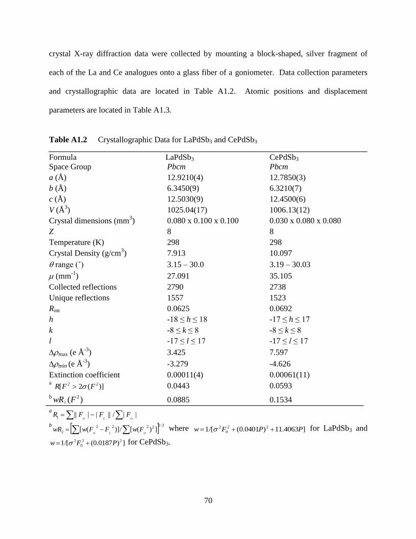
70
crystal X-ray diffraction data were collected by mounting a block-shaped, silver fragment of
each of the La and Ce analogues onto a glass fiber of a goniometer. Data collection parameters
and crystallographic data are located in Table A1.2. Atomic positions and displacement
parameters are located in Table A1.3.
Table A1.2 Crystallographic Data for LaPdSb3 and CePdSb3
Formula LaPdSb3 CePdSb3
Space Group Pbcm Pbcm
a (Å) 12.9210(4) 12.7850(3)
b (Å) 6.3450(9) 6.3210(7)
c (Å) 12.5030(9) 12.4500(6)
V (Å3) 1025.04(17) 1006.13(12)
Crystal dimensions (mm3) 0.080 x 0.100 x 0.100 0.030 x 0.080 x 0.080
Z 8 8
Temperature (K) 298 298
Crystal Density (g/cm3) 7.913 10.097
range (˚) 3.15 – 30.0 3.19 – 30.03
(mm-1
) 27.091 35.105
Collected reflections 2790 2738
Unique reflections 1557 1523
Rint 0.0625 0.0692
h -18 ≤ h ≤ 18 -17 ≤ h ≤ 17
k -8 ≤ k ≤ 8 -8 ≤ k ≤ 8
l -17 ≤ l ≤ 17 -17 ≤ l ≤ 17
max (e Å-3
) 3.425 7.597
min (e Å-3
) -3.279 -4.626
Extinction coefficient 0.00011(4) 0.00061(11) a )](2[ 22 FFR 0.0443 0.0593
b )( 22 FwR 0.0885 0.1534
a ||/||||||1 OCO
FFFR
b 2/12222
2 ])([/)]([ OCO
FwFFwwR where ]4063.11)0401.0(/[1 22
0
2 PPFw for LaPdSb3 and
])0187.0(/[1 22
0
2 PFw for CePdSb3.
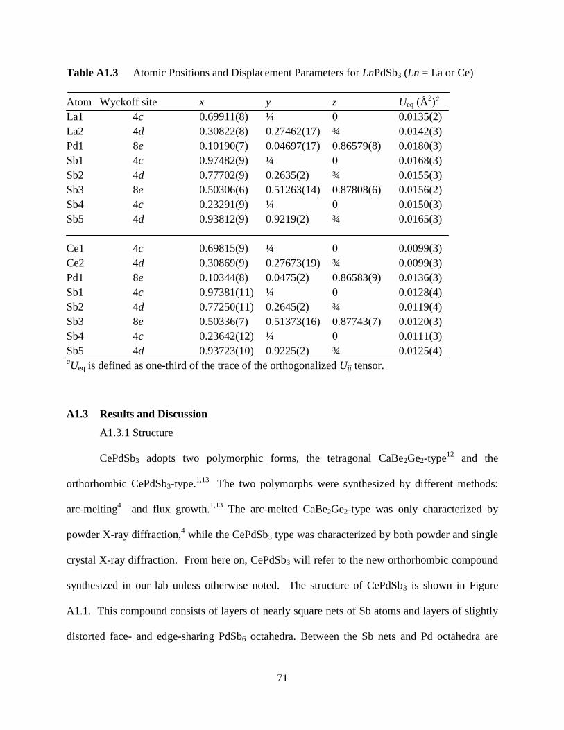
71
Table A1.3 Atomic Positions and Displacement Parameters for LnPdSb3 (Ln = La or Ce)
Atom Wyckoff site x y z Ueq (Å2)a
La1 4c 0.69911(8) ¼ 0 0.0135(2)
La2 4d 0.30822(8) 0.27462(17) ¾ 0.0142(3)
Pd1 8e 0.10190(7) 0.04697(17) 0.86579(8) 0.0180(3)
Sb1 4c 0.97482(9) ¼ 0 0.0168(3)
Sb2 4d 0.77702(9) 0.2635(2) ¾ 0.0155(3)
Sb3 8e 0.50306(6) 0.51263(14) 0.87808(6) 0.0156(2)
Sb4 4c 0.23291(9) ¼ 0 0.0150(3)
Sb5 4d 0.93812(9) 0.9219(2) ¾ 0.0165(3)
Ce1 4c 0.69815(9) ¼ 0 0.0099(3)
Ce2 4d 0.30869(9) 0.27673(19) ¾ 0.0099(3)
Pd1 8e 0.10344(8) 0.0475(2) 0.86583(9) 0.0136(3)
Sb1 4c 0.97381(11) ¼ 0 0.0128(4)
Sb2 4d 0.77250(11) 0.2645(2) ¾ 0.0119(4)
Sb3 8e 0.50336(7) 0.51373(16) 0.87743(7) 0.0120(3)
Sb4 4c 0.23642(12) ¼ 0 0.0111(3)
Sb5 4d 0.93723(10) 0.9225(2) ¾ 0.0125(4) aUeq is defined as one-third of the trace of the orthogonalized Uij tensor.
A1.3 Results and Discussion
A1.3.1 Structure
CePdSb3 adopts two polymorphic forms, the tetragonal CaBe2Ge2-type12
and the
orthorhombic CePdSb3-type.1,13
The two polymorphs were synthesized by different methods:
arc-melting4 and flux growth.
1,13 The arc-melted CaBe2Ge2-type was only characterized by
powder X-ray diffraction,4 while the CePdSb3 type was characterized by both powder and single
crystal X-ray diffraction. From here on, CePdSb3 will refer to the new orthorhombic compound
synthesized in our lab unless otherwise noted. The structure of CePdSb3 is shown in Figure
A1.1. This compound consists of layers of nearly square nets of Sb atoms and layers of slightly
distorted face- and edge-sharing PdSb6 octahedra. Between the Sb nets and Pd octahedra are a
La1 La2
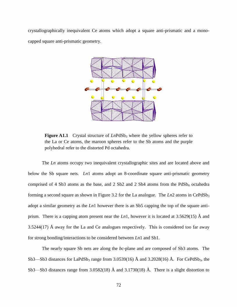
72
crystallographically inequivalent Ce atoms which adopt a square anti-prismatic and a mono-
capped square anti-prismatic geometry.
The Ln atoms occupy two inequivalent crystallographic sites and are located above and
below the Sb square nets. Ln1 atoms adopt an 8-coordinate square anti-prismatic geometry
comprised of 4 Sb3 atoms as the base, and 2 Sb2 and 2 Sb4 atoms from the PdSb6 octahedra
forming a second square as shown in Figure 3.2 for the La analogue. The Ln2 atoms in CePdSb3
adopt a similar geometry as the Ln1 however there is an Sb5 capping the top of the square anti-
prism. There is a capping atom present near the Ln1, however it is located at 3.5629(15) Å and
3.5244(17) Å away for the La and Ce analogues respectively. This is considered too far away
for strong bonding/interactions to be considered between Ln1 and Sb1.
The nearly square Sb nets are along the bc-plane and are composed of Sb3 atoms. The
Sb3—Sb3 distances for LaPdSb3 range from 3.0539(16) Å and 3.2028(16) Å. For CePdSb3, the
Sb3—Sb3 distances range from 3.0582(18) Å and 3.1730(18) Å. There is a slight distortion to
Figure A1.1 Crystal structure of LnPdSb3 where the yellow spheres refer to
the La or Ce atoms, the maroon spheres refer to the Sb atoms and the purple
polyhedral refer to the distorted Pd octahedra.
73
the nets, but they are not as distorted as CeNiSb3.14
The distorted angles in the Sb nets are
86.96(3)°and 92.95(3)° for LaPdSb3, and 86.71(4)° and 93.21(4)° for CePdSb3. In the similar
structure CeCrSb3, the Sb net angles are perfect 90.00°.15
The Pd environment of LnPdSb3 is a distorted octahedral environment. The Pd—Sb
distances range from 2.6781(13) – 2.8725(15) Å for LaPdSb3 and 2.6786(14) – 2.8228(18) Å for
CePdSb3. They are comparable to those found in the binary compound PdSb (NiAs-type) of
2.737 Å, in which Pd adopts an octahedral coordination.16
The Pd-centered octahedra in
LaPdSb3 and CePdSb3 are highly distorted with Sb—Pd—Sb angles as acute as 73.87(3)° and
73.79(3)°. The PdSb6 octahedra are edge sharing in the b-direction and are face-sharing in the c-
direction. The Pd—Pd distances are 2.895(2) Å in LaPdSb3 and 2.884(2) Å in CePdSb3 which
are comparable to the Pd-Pd distance of 2.751 Å in Pd metal.17
A1.4 References
(1) Thomas, E. L.; Gautreaux, D. P.; Chan, J. Y. Acta Crystallogr. Sect. E: Struct. Rep.
Online 2006, E62, i96-i98.
(2) Marazza, R.; Rossi, D.; Ferro, R. J. Less-Common Metals 1980, 75, P25-P28.
(3) Hofmann, W. K.; Jeitschko, W. Monatsh. Chem. 1985, 116, 569-580.
(4) Cava, R. J.; Ramirez, A. P.; Takagi, H.; Krajewski, J. J.; Peck, W. F. J. Magn. Magn.
Mater. 1993, 128, 124-128.
(5) Sologub, O.; Hiebl, K.; Rogl, P.; Noël, H.; Bodak, O. J. Alloys Compd. 1994, 210, 153-
157.
(6) Gordon, R. A.; DiSalvo, F. J.; Poettgen, R. J. Alloys Compd. 1995, 228, 16-22.
(7) Gordon, R. A.; DiSalvo, F. J. Z. Naturforsch. 1996, 51, 52-56.
(8) Gordon, R. A.; DiSalvo, F. J.; Poettgen, R.; Brese, N. E. J. Chem. Soc., Faraday Trans.
1996, 92, 2167-2171.
(9) Fisk, Z.; Hess, D. W.; Pethick, C. J.; Pines, D.; Smith, J. L.; Thompson, J. D.; Willis, J.
O. Science 1988, 239, 33-42.

74
(10) Cho, B. K.; Gordon, R. A.; Jones, C. D. W.; DiSalvo, F. J.; Kim, J. S.; Stewart, G. R.
Phys. Rev. B 1998, 57, 15191-15196.
(11) Muro, Y.; Takeda, N.; Ishikawa, M. J. Alloys Compd. 1997, 257, 23-29.
(12) Eisenmann, B.; Schaefer, H.; May, N.; Müller, W. Z. Naturforsch. B: Chem. Sci. 1972,
27, 1155-1157.
(13) Thamizhavel, A.; Nakashima, H.; Shiromoto, T.; Obiraki, Y.; Matsuda, T. D.; Haga, Y.;
Ramakrishnan, S.; Takeuchi, T.; Settai, R.; Onuki, Y. J. Phys. Soc. Jpn. 2005, 74, 2617-
2621.
(14) Macaluso, R. T.; Wells, D. M.; Sykora, R. E.; Albrecht-Schmitt, T. E.; Mar, A.;
Nakatsuji, S.; Lee, H.; Fisk, Z.; Chan, J. Y. J. Solid State Chem. 2004, 177, 293-298.
(15) Brylak, M.; Jeitschko, W. Z. Naturforsch. B: Chem. Sci. 1995, 50, 899-904.
(16) Pratt, J. N.; Myles, K. M.; Darby, J. B. J.; Mueller, M. H. J. Less-Common Metals 1968,
14, 427-433.
(17) Donohue, P. C. J. Solid State Chem. 1975, 12, 80-3.
75
APPENDIX 2 – EuCu9Sn4
A2.1 Introduction
Many compounds of the NaZn13 structure type have received attention because of the
remarkable properties they exhibit. UBe13, a heavy fermion superconductor, has an enormous
specific heat coefficient of γ = 1100 mJ mol-1
K-2
.1 LaCo13 possesses the large ordering
temperature TN = 1290 °C.2 In 1994, a tetragonal derivative of the NaZn13 structure was
discovered in LaFe9Si4.3 Many analogues adopting this tetragonal structure have been studied.
Magnetic properties of LnCu9Sn4 compounds (Ln = La – Nd) all order ferromagnetically from 5
– 15 while no magnetic ordering is observed down to 1.5 K in LnCu9.4Sn3.6, which adopts the
cubic NaZn13 structure type.4 The atomic ordering of the tetragonal structure leads to magnetic
ordering, while the disorder in the cubic LnCu9.4Sn3.6 hinders any magnetic order down to 2 K.4
Recently, the structure and magnetic properties of EuCu9Sn4, EuCu4Sn2, and EuCuSn2 were
reported.5 In our effort to continue the exploration of the Ln – Cu – Sn phase space, high quality
single crystals of EuCu9Sn4 were grown by Sn flux to study the transport properties of this
structure type. The synthesis, crystal structure determination, and physical properties of high
quality single crystals of EuCu9Sn4 are discussed herein.
A2.2 Experimental
A2.2.1 Synthesis
Single crystals of EuCu9Sn4 were synthesized using a Sn flux growth method. Eu pieces
(99.9%, Alfa Aesar), Cu powder (99.999%, Alfa Aesar), and Sn shot (99.99%, Alfa Aesar) were
placed into an alumina crucible in a 1:1:20 stoichiometric ratio. After sealing the crucible into
an evaculated fused-silica tube, the entire reaction vessel was placed into a furnace for heat
treatment. The sample was heated at 1150 °C for 48 h followed by a slow-cooling at 5 °C/h
down to 300 °C. After the sample temperature reached 300 °C, the excess flux was removed by

76
centrifugation. The sample contained thin metallic plates, which were determined to be
EuCu9Sn4. There is no surface degradation to the crystal visible over a period of months. Some
of the crystals contained small amounts of Sn present on the surface which were removed
mechanically.
A2.2.2 Single Crystal X-Ray Diffraction
Single crystal X-ray diffraction was performed on a crystal with dimensions of 0.025 x
0.1 x 0.125 mm3. The crystal was mounted onto the glass fiber of the goniometer with epoxy
and data were collected on a Nonius Kappa CCD X-ray diffractometer (MoKα = 0.71073 Å).
The unit cell parameters were determined from images taken at a rotation of 15 °φ. The
structural model was solved by direct methods using SIR92 6 and refined using SHELXL97.
7
The data were corrected for absorption and the displacement parameters were refined as
anisotropic. Crystallographic data and data collection parameters are listed in Table A2.1 and
atomic positions and anisotropic displacement parameters are listed in Table A2.2.
Table A2.1 Crystallographic Data for EuCu9Sn4
Formula EuCu9Sn4
Formula Units (amu) 1198.58
Space Group I4/mcm
a (Å) 8.641(2)
c (Å) 12.433(3)
V (Å) 928.3(4)
Crystal Size (mm3) 0.03/0.10/0.13
Z 4
Temperature (°C) 20(2)
Density (g cm-1
) 8.576
θ Range (°) 3.28-30.03
μ (mm-1
) 37.254
Rint 0.0455
Collected Reflections 1058
Unique Reflections 390
h -12 ≤ h ≤ 12
k -8 ≤ k ≤ 8
l -17 ≤ l ≤ 13

77
Table A2.1 (cont.)
∆ρmax (e Å-3
) 2.569
∆ρmin (e Å-3
) -2.425
Extinction coefficient 0.0038(5) a )](2[ 22 FFR 0.0441
b )( 2
2 FwR 0.1282
a 001 /)( FFFFR c
b 2/122
0
22
0
2
0 ])([/)]([)( FwFFwFR cw ;where ]12.4528)0.0850()(/[1 22
0
2 PPFw
Table A2.2 Atomic Positions and Displacement Parameters for EuCu9Sn4
Atom Wyckoff Site x y z Ueq (Å2)a
Eu1 4a 0 0 ¼ 0.01318
Cu1 16l 0.108912 0.608912 0.174330 0.01376
Cu2 16k 0.798244 0.944009 0 0.01561
Cu3 4d 0 ½ 0 0.01186
Sn1 16l 0.315068 0.815065 0.125358 0.01106 a Ueq is defined as one-third of the trace of the orthogonalized Uij tensor.
A2.2.3 Physical Property Measurements
Magnetic measurements on single crystals of EuCu9Sn4 were performed using a Quantum
Desing MPMS Superconducting Quantum Interference Device (SQUID) magnetometer.
Temperature-dependent susceptibility data were measured at an applied field of 0.1 T from 2 K –
300 K and the field-dependent magnetization data were measured at 2 K up to 7 T. Transport
property measurements were conducted using a Quantum Design Physical Property
Measurement System (PPMS) at ambient pressure. Resistivity data were measured at 0 T, 0.5 T
and 9 T while magnetoresistance data up to 9 T were measured at 2 K.
A2.3 Results and Discussion
A2.3.1 Structure
EuCu9Sn4 crystallizes in the tetragonal space group I4/mcm (# 140) with lattice
parameters of a = 8.641(2) Å and c = 12.433(3) Å. This is in agreement with the EuCu9Sn4

78
lattice parameters a = 8.633(2) Å and c = 12.425(2) Å reported by Mazzone et al.5 The current
work was all ready in progress before the Mazzone paper was published in early 2008.
EuCu9Sn4 adopts the LaFe9Si4 structure type which is a distorted variation of the cubic NaZn13
structure type.3,8
There are five atomic positions in the EuCu9Sn4 structure: Eu1, Cu1, Cu2, Cu3,
and Sn1 which are listed in Table A2.2 with the displacement parameters. The structure shown
in Figure A2.1 consists of alternating layers of Cu3 icosahedra and slightly irregular Eu snub-
cubes. Figure A2.1 (b) highlights the Cu3 and Eu environments. Table A2.3 displays selected
interatomic distances within the Cu3 and Eu subunits. Though similar, the distances vary
slightly confirming that both the Cu3 iscoahedra and Eu snub-cubes are somewhat distorted.
The Eu analogue does not follow the lanthanide contraction seen in other LnCu9Sn4 compounds
(Ln = La – Nd) suggesting that Eu may have an oxidation state of +2 in this compound.4
c
a
Eu
Cu
Sn
Eu Environment
CN = 24
Cu3 Environment
CN = 12
Cu1 Cu1
Cu1Cu1
Cu2Cu2
Cu2Cu2
Cu2
Cu2
Cu1
Cu1
(a) (b)
Figure A2.1 (a) Crystal structure of EuCu9Sn4 viewed down the b axis. (b)
Images of environments of Cu3 icosahedra and Eu distorted snub-cubes.

79
Table A2.3 Selected Interatomic Distances (Å) of EuCu9Sn4 Subunits
Eu Irregular Snub Cube Cu3-Icosahedra
Eu1-Sn1(x8) 3.5167(8) Cu3-Sn1(x4) 2.7453(9)
Eu1-Cu1(x8) 3.6320(10) Cu3-Cu1(x4) 2.5434(15)
Eu1-Cu2(x8) 3.5965(10) Cu3-Cu2(x4) 2.6222(15)
A2.3.2 Physical Properties
The magnetic susceptibility of EuCu9Sn4 was measured from 2 – 300 K with an applied
field of 0.1 T for several single crystals aligned side-by-side. Figure A2.2 displays the
susceptibility data from 2 – 50 K and the inset shows the inverse susceptibility plot. EuCu9Sn4
orders ferromagnetically at ~ 10 K. This is in agreement with the published magnetic data where
this compound also shows ferromagnetic ordering at 10 K.5 The experimental effective magnetic
moment was determined from a Curie-Weiss fit of the inverse data from 50 – 300 K. The
experimental moment of 6.48 µB is close to the calculated moment for Eu2+
of 7.93. This is
0
1
2
3
4
0 10 20 30 40 50
M/H
(e
mu
/mo
l E
u)
T (K)
0
10
20
30
40
50
60
0 50 100 150 200 250 300
1/
T (K)
Figure A2.2 Magnetic Susceptibility of EuCu9Sn4 measured with an applied
field of 0.1 T from 2 – 300 K. Data from 2 – 50 K were shown to enhance the
ordering seen below 20 K. The inset displays the inverse susceptibity.
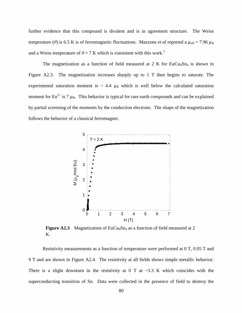
80
further evidence that this compound is divalent and is in agreement structure. The Weiss
temperature (θ) is 6.5 K is of ferromagnetic fluctuations. Mazzone et al reported a µeff = 7.96 µB
and a Weiss temperature of θ = 7 K which is consistent with this work.5
The magnetization as a function of field measured at 2 K for EuCu9Sn4 is shown in
Figure A2.3. The magnetization increases sharply up to 1 T then begins to saturate. The
experimental saturation moment is ~ 4.4 µB which is well below the calculated saturation
moment for Eu2+
is 7 µB. This behavior is typical for rare earth compounds and can be explained
by partial screening of the moments by the conduction electrons. The shape of the magnetization
follows the behavior of a classical ferromagnet.
Resistivity measurements as a function of temperature were performed at 0 T, 0.05 T and
9 T and are shown in Figure A2.4. The resistivity at all fields shows simple metallic behavior.
There is a slight downturn in the resistivity at 0 T at ~3.3 K which coincides with the
superconducting transition of Sn. Data were collected in the presence of field to destroy the
0
1
2
3
4
5
0 1 2 3 4 5 6 7
M (
B/m
ol E
u)
H (T)
T = 2 K
Figure A2.3 Magnetization of EuCu9Sn4 as a function of field measured at 2
K.
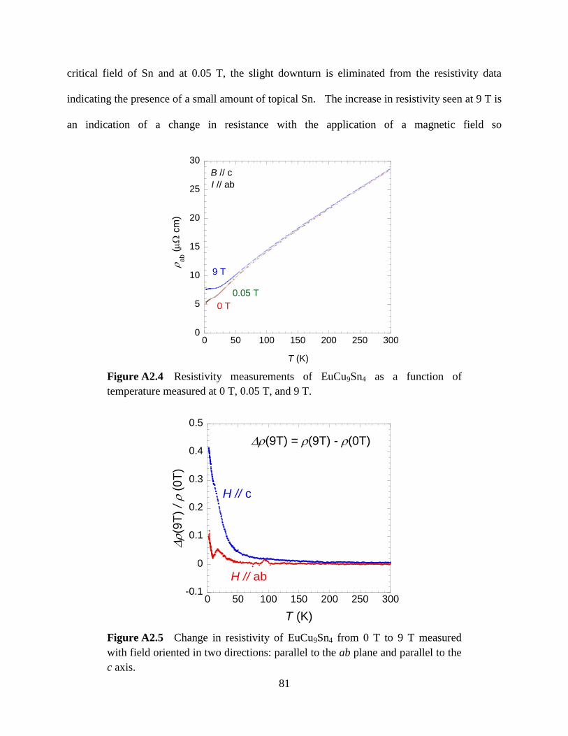
81
critical field of Sn and at 0.05 T, the slight downturn is eliminated from the resistivity data
indicating the presence of a small amount of topical Sn. The increase in resistivity seen at 9 T is
an indication of a change in resistance with the application of a magnetic field so
-0.1
0
0.1
0.2
0.3
0.4
0.5
0 50 100 150 200 250 300
(9
T)
/ (
0T
)
T (K)
H // c
H // ab
(9T) = (9T) - (0T)
Figure A2.5 Change in resistivity of EuCu9Sn4 from 0 T to 9 T measured
with field oriented in two directions: parallel to the ab plane and parallel to the
c axis.
0
5
10
15
20
25
30
0 50 100 150 200 250 300
a
b (
cm
)
T (K)
9 T
0 T
0.05 T
B // c
I // ab
Figure A2.4 Resistivity measurements of EuCu9Sn4 as a function of
temperature measured at 0 T, 0.05 T, and 9 T.
82
magnetoresistance was measured. Figure A2.5 shows the change in resistivity from 0 T to 9 T as
a function of temperature. When the magnetic field is applied parallel to the c axis of the crystal,
the magnetoresistance is ~ 40 % at 2 K. When the magnetic field is applied parallel to the ab-
plane of the crystal, the change in resistivity is not as large. This is further evidence of the
highly anisotropic nature of these crystals.
A2.4 References
(1) Ott, H. R.; Rudigier, H.; Fisk, Z.; Smith, J. L. Phys. Rev. Lett. 1983, 50, 1595-1598.
(2) Velge, W. A. J. J.; Buschow, K. H. J. J. Appl. Phys. 1968, 39, 1717-1720.
(3) Tang, W.; Liang, J.; Chen, X.; Rao, G. J. Appl. Phys. 1994, 76, 4095-4098.
(4) Singh, S.; Fornasini, M. L.; Manfrinetti, P.; Palenzona, A.; Dhar, S. K.; Paulose, P. L. J.
Alloys Compd. 2001, 317-318, 560-566.
(5) Mazzone, D.; Paulose, P. L.; Dhar, S. K.; Fornasini, M. L.; Manfrinetti, P. J. Alloys
Compd. 2008, 2008.
(6) Altomare, A.; Cascarno, G. L.; Giacovazzo, A.; Guagliardi, A. J. Appl. Crystallogr.
1993, 26, 343-350.
(7) Sheldrick, G. M.; University of Gottingen: Germany, 1997.
(8) Shoemaker, D. P.; Marsh, R. E.; Ewing, F. J.; Pauling, L. Acta Cryst. 1952, 5, 637-644.
83
APPENDIX 3 –STRUCTURAL DETERMINATION OF VB2
A3.2 Introduction
Transition metal diborides have been extensively studied for many years. However the
recent discovery of superconducting behavior of MgB2 at 39 K has refueled the interest in these
simple diborides.2 Transition metal diborides exist for all first row transition metals between Sc
– Fe. The wide range of isostructural compounds make this structure type intriguing because of
the chance to study the property changes throughout all the isostructural compounds. Recently,
our collaborators discovered that VB2 has a very large magnetoresistance of ~ 1100 % at low
temperatures.1 This extremely large magnetoresistive behavior is highly dependent on the
quality of the single crystals measured.1 To gain better insight into the properties of this
structure, very accurate lattice parameters were needed for energy band calculations and to
determine the Fermi surface of VB2. Therefore the single crystal X-ray diffraction data of VB2
were collected at 293 K and 90 K on high quality single crystals and the results are reported
herein.
A3.2 Experimental and Results
High quality single crystals of VB2 were synthesized by Al flux by collaborators in the
Department of Physics and Astronomy at Louisiana State University.1 The crystals grew as both
rods and plates and powder X-ray diffraction was used to confirm that the sample was single
phase. Powder X-ray diffraction data were collected on a Bruker D8 Advance Diffractometer
with monochromatic Cu K radiation ( = 1.540562 Å) at room temperature and it was
determined that both crystal morphologies are VB2. Accurate lattice parameters were needed for
energy band calculations, therefore the single crystal X-ray diffraction data were collected at 293
1 Portions of this chapter reprinted by permission of The Institute of Physics: Karki, A.B.; Gautreaux, D.P.;
Chan, J.Y.; Harrison, N.; Browne, D.A.; Goodrich, R.G.; Young, D.P.; “Magnetotransport Properties and the
Fermi Surface of Single Crystal VB2”, J.Phys: Condens. Matter. 2008, 20, 035209.

84
K and 90 K. A 0.05 x 0.075 x 0.125 mm3 crystal fragment was glued to a glass fiber with epoxy
and mounted on the goniometer of a Nonius Kappa CCD diffractometer equipped with Mo Kα
radiation (λ = 0.71073 Å). For low temperature data collections, the crystal was mounted onto
the fiber using vacuum grease and no epoxy was used. The temperature was regulated with a
cooled nitrogen gas stream produced by an Oxford Cryostream Cooler. Initial unit cell
parameters were determined from images taken at a rotation of 15 °φ. The structural model was
solved by direct methods using SIR973 and refined using SHELXL97.
4 The data were corrected
for absorption and the displacement parameters were refined as anisotropic. Selected
crystallographic data and data collection parameters are listed in Table A3.1. Atomic positions
and anisotropic displacement parameters are listed in Table A3.2 for both data collections. VB2
adopts the well known AlB2 structure type and is displayed in Figure A3.1. The structure
consists of alternating layers of vanadium atoms and graphite like sheets of boron. There are no
structural discrepancies between our VB2 structure and the known AlB2 structure type. The
structural information obtained from this study was used for energy band calculations and the
results are reported in the Journal of Physics: Condensed Matter.
Table A3.1 Crystallographic Data for VB2
Sample AK104 AK104
Space Group P6/mmm P6/mmm
Temperature (K) 293 90
a (Å) 3.0000(4) 2.9980(10)
b (Å) 3.0000(4) 2.9980(10)
c (Å) 3.0620(8) 3.044(2)
V (Å3) 23.866(8) 23.69(2)
Z 1 1
Density (g cm-1
) 5.049 5.085
Range (°) 7.86-29.55 6.70-29.57
μ (mm-1
) 9.274 9.341
max (e Å-3
) 0.697 0.690
min (e Å-3
) -0.428 -0.521

85
TableA3.1 (cont.) a )](2[ 22 FFR 0.0188 0.0252
b )( 2
2 FwR 0.0400 0.0563 a 001 /)( FFFFR c
b 2/122
0
22
0
2
0 ])([/)]([)( FwFFwFR cw ;where ])0.0167()(/[1 22
0
2 PFw ,
])0.1000()(/[1 22
0
2 PFw , for 293 K and 90 K respectively
Table A3.2 Atomic Positions and Displacement Parameters for VB2
Atom Wyckoff Site x y z Ueq (Å2)
a
293 K
V1 1a 0 0 ¼ 0.0033(16)
B1 2d ⅓ ⅔ ½ 0.000(2)
90 K
V1 1a 0 0 ¼ 0.0033(16)
B1 2d ⅓ ⅔ ½ 0.0036(19) a Ueq is defined as one-third of the trace of the orthogonalized Uij tensor.
A3.2 References
(1) Karki, A. B.; Gautreaux, D. P.; Chan, J. Y.; Harrison, N.; Browne, D.; Goodrich, R. G.;
Young, D. P. J. Phys.: Condens. Matter 2008, 20, 035209.
(2) Nagamatsu, J.; Nakagawa, N.; Muranaka, T.; Zenitani, Y.; Akimitsu, J. Nature 2001,
410, 63-64.
V
B
a b
c
a
b
(a) (b)
Figure A3.1 (a) Layered crystal structure of VB2 viewed in the [110]
direction. (b) View down the c-axis of the crystal structure of VB2.

86
(3) Altomare, A.; Burla, M. C.; Camalli, M.; Cascarno, G. L.; Giacovazzo, A.; Guagliardi,
A.; Moliterni, A. G. G.; Polidori, G.; Spagna, R. J. J. Appl. Crystallogr. 1999, 32, 115-
119.
(4) Sheldrick, G. M.; University of Gottingen: Germany, 1997.

87
APPENDIX 4 – Y2-xCexTi2O7
A4.1 Introduction
Many research groups are focused on finding alternative fuel sources because of the
uncertainty of the world’s supply of fossil fuels. An appealing alternative fuel source is
hydrogen because it is abundantly found in H2O. Splitting of H2O by means such as
photocatalysis or electrocatalysis would yield the desired H2 product. CeO2 is used in
automobile catalytic converters and has the ability to release O2 (2 CeO2 Ce2O3 + ½ O2).1
This ability to release O2 might suggest applications of CeO2 as a water oxidation catalyst. Solid
oxides are ideal materials for water oxidation electrodes because they are likely to be inert under
the high positive potentials required.
There are very few practical electrocatalytic materials for generating H2 by the oxidation
of H2O and catalysts of this reaction are of great interest. The introduction of Ce into Y2Ti2O7
may also introduce redox activity, therefore, samples of Y2-xCexTi2O7 were synthesized for the
investigation of their electrocatalytic behavior. A complete solid solution is not expected
because the end members of the series, Y2Ti2O7 and Ce2Ti2O7, adopt cubic and monoclinic
structure respectively.2,3
Powder neutron diffraction data and physical properties are reported
herein for Y2-xCexTi2O7 (nominal x = 0, 0.15, 0.35).
A4.2 Experimental and Results
A4.2.1 Synthesis
Y2-xCexTi2O7 (x = 0, 0.15, 0.35) compounds have been synthesized using solid state
ceramic synthesis. Samples are prepared using a combination of grinding and mixing the
constituent oxide powders, then pressing a pellet of the resulting mixture. The amounts of
reactant oxide powders needed to make ~7 g of product were obtained using the following
reaction: 2 TiO2 + x CeO2 + (2−𝑥
2) Y2O3 Y2-xCexTi2O7. Each sample was mixed and pressed

88
into a pellet with a diameter of ~ 10 mm. The pellets were then dwelled at temperatures of 1000
°C, 1100 °C, 1300 °C, 1400 °C, and 1450 °C. The samples remained at each temperature for ~ 2
days with intermittent grinding and repressing of the pellet between each heat treatment. Powder
X-ray diffraction patterns were measured between each heat treatment to determine if the phase
assemblage has reached equilibrium.
A4.2.2 Neutron Powder Diffraction
Neutron powder diffraction (NPD) data were collected for all samples on BT-1 with a
Cu(311) monochromator (λ = 1.5403 Å). Experimental and statistical data are provided in Table
A4.1. The NPD data were refined using Rietveld refinement. The observed NPD data are in
very good agreement with the calculated NPD data and are shown in Figure A4.1. There are
some small impurity peaks (< 4%), which can be attributed to a rutile TiO2 impurity. The Y2-
xCexTi2O7 (x = 0, 0.34, and 0.62) compounds crystallize in the cubic space group Fd 3 m (No.
227, origin choice 2). The atomic positions and thermal parameters for all three compounds are
shown in Table A4.2. There are no oxygen deficiencies in any of the pyrochlore compounds.
The Ce atoms occupy the 16c site which was expected based on the ionic radii of the atoms in
the compound. Although Ce2Ti2O7 adopts a monoclinic structure type, the introduction of Ce
ions at x < 0.63 into the cubic pyrochlore structure does not induce any structural phase changes.
Table A4.1 Experimental and Statistical Neutron Data for Y2-xCexTi2O7
Nominal Composition Y2Ti2O7 Y1.85Ce0.15Ti2O7 Y1.65Ce0.35Ti2O7
Observed Composition Y2Ti2O7 Y1.66Ce0.34Ti2O7 Y1.37Ce0.63Ti2O7
Chi2 1.849 2.223 2.285
Rp 3.96 3.82 4.05
wRp 4.82 4.49 5.04
a (Å) 10.09983(18) 10.10634(17) 10.11409(5)
TiO2 (% wt) 3.21 1.95 0.18221

89
Figure A4.1 Neutron powder diffraction patterns of (a) Y2Ti2O7, (b)
Y1.66Ce0.34Ti2O7, and (c) Y1.37Ce0.63Ti2O7 where the red crosses are the
observed NPD pattern, solid black tick marks are the calculated NPD profiles
of Y2-xCexTi2O7, solid red tick marks are the calculated NPD profiles of rutile
TiO2, and magenta patterns are the difference NPD profiles for Y2-xCexTi2O7.
Y2Ti2O7
Y1.66Ce0.34Ti2O7
Y1.37Ce0.63Ti2O7
(a)
(b)
(c)

90
Table A4.2 Atomic Positions and Thermal Parameters of Y2-xCexTi2O7
Atom Wyckoff Site x y z Occupancy Uiso
Y2Ti2O7
Y 16c 0 0 0 1.0 0.00859(18)
Ti 16d ½ ½ ½ 1.0 0.00506(30)
O1 48f 0.420986(61) ⅛ ⅛ 1.0 0.00811(13)
O2 8a ⅛ ⅛ ⅛ 1.0 0.00564(28)
Y1.66Ce0.34Ti2O7
Y 16c 0 0 0 0.830(11) 0.00779(22)
Ce 16c 0 0 0 0.170(11) 0.00779(22)
Ti 16d ½ ½ ½ 1.0 0.00593(27)
O1 48f 0.421195(51) ⅛ ⅛ 1.0 0.00884(13)
O2 8a ⅛ ⅛ ⅛ 1.0 0.00579(24)
Y1.37Ce0.63Ti2O7
Y 16c 0 0 0 0.686(12) 0.00921(28)
Ce 16c 0 0 0 0.314(12) 0.00921(28)
Ti 16d ½ ½ ½ 1.0 0.00762(33)
O1 48f 0.420986(61) ⅛ ⅛ 1.0 0.01082(15)
O2 8a ⅛ ⅛ ⅛ 1.0 0.00659(28)
A4.2.3 Physical Properties
The magnetic susceptibility and electrical resistivity of Y2-xCexTi2O7 (x = 0, 0.34, 0.63)
were measured. Y2-xCexTi2O7 (x = 0, 0.34, 0.63) were all insulators. The magnetic susceptibility
data was measured at 0.1 T for Y1.66Ce0.34Ti2O7 and Y1.37Ce0.63Ti2O7 and are displayed in Figure
A4.2. Both Y1.66Ce0.34Ti2O7 and Y1.37Ce0.63Ti2O7 are paramagnetic down to 2 K and Y2Ti2O7 is
not magnetic. Effective moments of 0.44 µB and 0.55 µB were obtained from a modified Curie-
Weiss fit of the data from 2 – 275 K for Y1.66Ce0.34Ti2O7 and Y1.37Ce0.63Ti2O7 respectively. A
modified Curie-Weiss fit was used because the inverse susceptibility plots were not linear. The
calculated magnetic moment for a Ce3+
ion is 2.54 µB, while Ce4+
is not magnetic. Weiss
temperatures (θ) of -0.81 K and -1.01 K were obtained for Y1.66Ce0.34Ti2O7 and Y1.37Ce0.63Ti2O7
respectively. The field-dependent magnetization data were measured for both compounds at 3 K
and are shown in Figure A4.3. The magnetization of both compounds do not saturate in
magnetic fields up to 9 T. The magnetization is well below the saturation moment for Ce3+
of
2.14 µB.
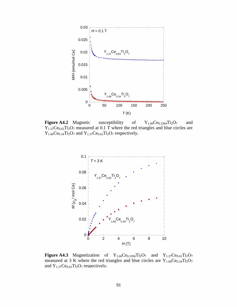
91
0
0.02
0.04
0.06
0.08
0.1
0 2 4 6 8 10
M (
B/ m
ol C
e)
H (T)
Y1.37
Ce0.63
Ti2O
7
Y1.66
Ce0.34
Ti2O
7
T = 3 K
Figure A4.3 Magnetization of Y1.66Ce0.3394Ti2O7 and Y1.37Ce0.63Ti2O7
measured at 3 K where the red triangles and blue circles are Y1.66Ce0.34Ti2O7
and Y1.37Ce0.63Ti2O7 respectively.
0
0.005
0.01
0.015
0.02
0.025
0.03
0 50 100 150 200 250
M/H
(em
u/m
ol C
e)
T (K)
Y1.66
Ce0.34
Ti2O
7
Y1.37
Ce0.63
Ti2O
7
H = 0.1 T
Figure A4.2 Magnetic susceptibility of Y1.66Ce0.3394Ti2O7 and
Y1.37Ce0.63Ti2O7 measured at 0.1 T where the red triangles and blue circles are
Y1.66Ce0.34Ti2O7 and Y1.37Ce0.63Ti2O7 respectively.
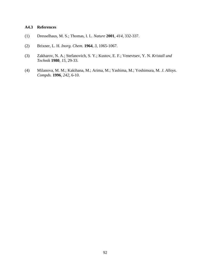
92
A4.3 References
(1) Dresselhaus, M. S.; Thomas, I. L. Nature 2001, 414, 332-337.
(2) Brixner, L. H. Inorg. Chem. 1964, 3, 1065-1067.
(3) Zakharov, N. A.; Stefanovich, S. Y.; Kustov, E. F.; Venevtsev, Y. N. Kristall und
Technik 1980, 15, 29-33.
(4) Milanova, M. M.; Kakihana, M.; Arima, M.; Yashima, M.; Yoshimura, M. J. Alloys.
Compds. 1996, 242, 6-10.
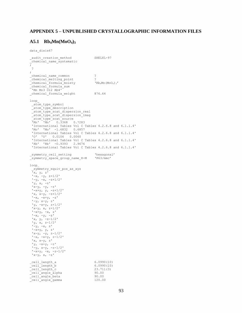
93
APPENDIX 5 – UNPUBLISHED CRYSTALLOGRAPHIC INFORMATION FILES
A5.1 Rb4Mn(MoO4)3
data_dixie67
_audit_creation_method SHELXL-97
_chemical_name_systematic
;
?
;
_chemical_name_common ?
_chemical_melting_point ?
_chemical_formula_moiety ‘Rb4Mn(MoO4)3’
_chemical_formula_sum
'Mn Mo3 O12 Rb4'
_chemical_formula_weight 876.64
loop_
_atom_type_symbol
_atom_type_description
_atom_type_scat_dispersion_real
_atom_type_scat_dispersion_imag
_atom_type_scat_source
'Mn' 'Mn' 0.3368 0.7283
'International Tables Vol C Tables 4.2.6.8 and 6.1.1.4'
'Mo' 'Mo' -1.6832 0.6857
'International Tables Vol C Tables 4.2.6.8 and 6.1.1.4'
'O' 'O' 0.0106 0.0060
'International Tables Vol C Tables 4.2.6.8 and 6.1.1.4'
'Rb' 'Rb' -0.9393 2.9676
'International Tables Vol C Tables 4.2.6.8 and 6.1.1.4'
_symmetry_cell_setting ‘hexagonal’
_symmetry_space_group_name_H-M ‘P63/mmc’
loop_
_symmetry_equiv_pos_as_xyz
'x, y, z'
'-x, -y, z+1/2'
'-y, -x, -z+1/2'
'y, x, -z'
'x-y, -y, -z'
'-x+y, y, -z+1/2'
'x, x-y, -z+1/2'
'-x, -x+y, -z'
'-y, x-y, z'
'y, -x+y, z+1/2'
'x-y, x, z+1/2'
'-x+y, -x, z'
'-x, -y, -z'
'x, y, -z-1/2'
'y, x, z-1/2'
'-y, -x, z'
'-x+y, y, z'
'x-y, -y, z-1/2'
'-x, -x+y, z-1/2'
'x, x-y, z'
'y, -x+y, -z'
'-y, x-y, -z-1/2'
'-x+y, -x, -z-1/2'
'x-y, x, -z'
_cell_length_a 6.0990(10)
_cell_length_b 6.0990(10)
_cell_length_c 23.711(3)
_cell_angle_alpha 90.00
_cell_angle_beta 90.00
_cell_angle_gamma 120.00

94
_cell_volume 763.8(2)
_cell_formula_units_Z 2
_cell_measurement_temperature 293(2)
_cell_measurement_reflns_used ?
_cell_measurement_theta_min ?
_cell_measurement_theta_max ?
_exptl_crystal_description ‘plate shaped fragment’
_exptl_crystal_colour ‘light brown’
_exptl_crystal_size_max 0.075
_exptl_crystal_size_mid 0.075
_exptl_crystal_size_min 0.025
_exptl_crystal_density_meas ?
_exptl_crystal_density_diffrn 3.812
_exptl_crystal_density_method 'not measured'
_exptl_crystal_F_000 790
_exptl_absorpt_coefficient_mu 15.922
_exptl_absorpt_correction_type ‘multi-scan’
_exptl_absorpt_correction_T_min ?
_exptl_absorpt_correction_T_max ?
_exptl_absorpt_process_details 'HKL Scalepack (Otwinowski & Minor 19'
_exptl_special_details
;
?
;
_diffrn_ambient_temperature 293(2)
_diffrn_radiation_wavelength 0.71073
_diffrn_radiation_type MoK\a
_diffrn_radiation_source 'fine-focus sealed tube'
_diffrn_radiation_monochromator graphite
_diffrn_measurement_device_type 'KappaCCD'
_diffrn_measurement_method ' \w scans \k offsets'
_diffrn_detector_area_resol_mean ?
_diffrn_standards_number 0
_diffrn_standards_interval_count ?
_diffrn_standards_interval_time ?
_diffrn_standards_decay_% none
_diffrn_reflns_number 2762
_diffrn_reflns_av_R_equivalents 0.0531
_diffrn_reflns_av_sigmaI/netI 0.0379
_diffrn_reflns_limit_h_min -8
_diffrn_reflns_limit_h_max 8
_diffrn_reflns_limit_k_min -6
_diffrn_reflns_limit_k_max 6
_diffrn_reflns_limit_l_min -32
_diffrn_reflns_limit_l_max 32
_diffrn_reflns_theta_min 3.44
_diffrn_reflns_theta_max 29.98
_reflns_number_total 489
_reflns_number_gt 376
_reflns_threshold_expression >2sigma(I)
_computing_data_collection 'COLLECT (Nonius, 2000)'
_computing_cell_refinement 'Denzo and Scalepack (Otwinowski & Minor, 1997)'
_computing_data_reduction 'Denzo and Scalepack (Otwinowski & Minor, 1997)'
_computing_structure_solution 'SHELXS-97 (Sheldrick, 1990)'
_computing_structure_refinement 'SHELXL-97 (Sheldrick, 1997)'
_computing_molecular_graphics ?
_computing_publication_material 'SHELXL-97 (Sheldrick, 1997)'
_refine_special_details
;
Refinement of F^2^ against ALL reflections. The weighted R-factor wR and
goodness of fit S are based on F^2^, conventional R-factors R are based
on F, with F set to zero for negative F^2^. The threshold expression of
F^2^ > 2sigma(F^2^) is used only for calculating R-factors(gt) etc. and is
not relevant to the choice of reflections for refinement. R-factors based
on F^2^ are statistically about twice as large as those based on F, and R-
factors based on ALL data will be even larger.
_refine_ls_structure_factor_coef Fsqd
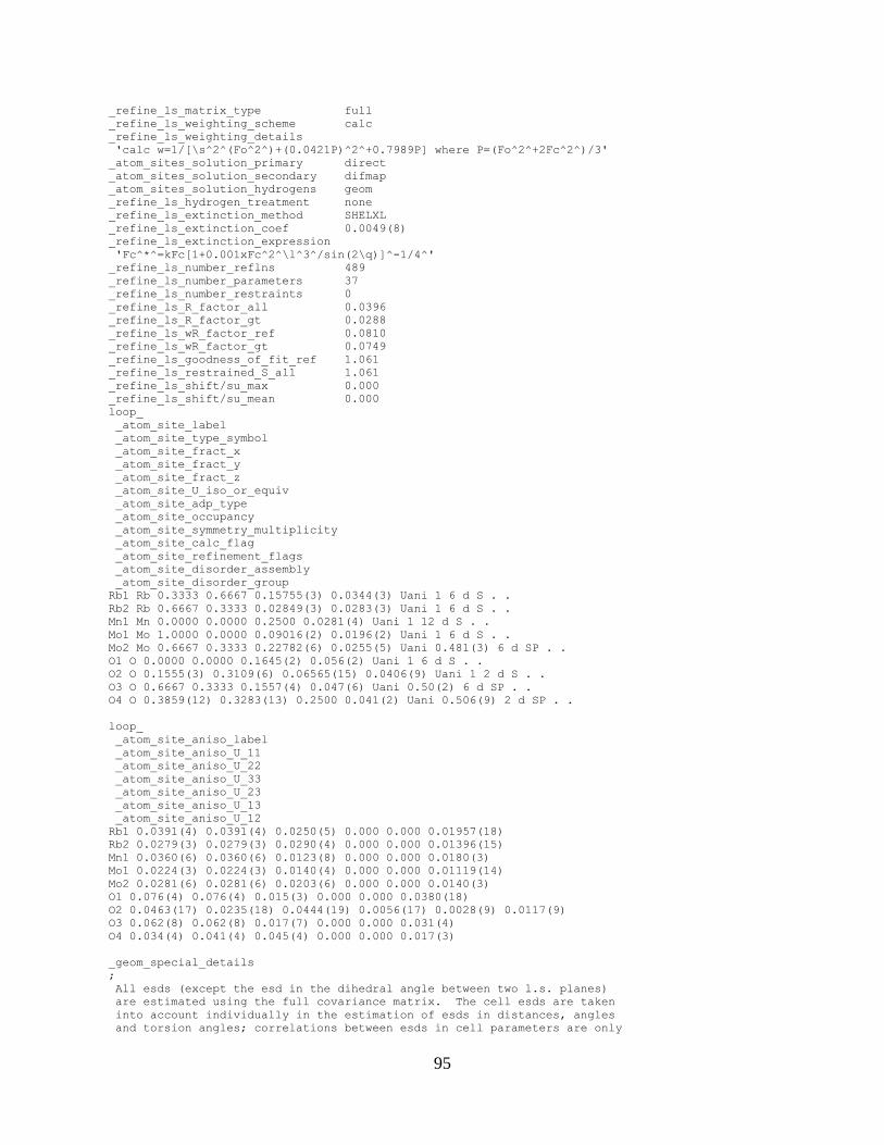
95
_refine_ls_matrix_type full
_refine_ls_weighting_scheme calc
_refine_ls_weighting_details
'calc w=1/[\s^2^(Fo^2^)+(0.0421P)^2^+0.7989P] where P=(Fo^2^+2Fc^2^)/3'
_atom_sites_solution_primary direct
_atom_sites_solution_secondary difmap
_atom_sites_solution_hydrogens geom
_refine_ls_hydrogen_treatment none
_refine_ls_extinction_method SHELXL
_refine_ls_extinction_coef 0.0049(8)
_refine_ls_extinction_expression
'Fc^*^=kFc[1+0.001xFc^2^\l^3^/sin(2\q)]^-1/4^'
_refine_ls_number_reflns 489
_refine_ls_number_parameters 37
_refine_ls_number_restraints 0
_refine_ls_R_factor_all 0.0396
_refine_ls_R_factor_gt 0.0288
_refine_ls_wR_factor_ref 0.0810
_refine_ls_wR_factor_gt 0.0749
_refine_ls_goodness_of_fit_ref 1.061
_refine_ls_restrained_S_all 1.061
_refine_ls_shift/su_max 0.000
_refine_ls_shift/su_mean 0.000
loop_
_atom_site_label
_atom_site_type_symbol
_atom_site_fract_x
_atom_site_fract_y
_atom_site_fract_z
_atom_site_U_iso_or_equiv
_atom_site_adp_type
_atom_site_occupancy
_atom_site_symmetry_multiplicity
_atom_site_calc_flag
_atom_site_refinement_flags
_atom_site_disorder_assembly
_atom_site_disorder_group
Rb1 Rb 0.3333 0.6667 0.15755(3) 0.0344(3) Uani 1 6 d S . .
Rb2 Rb 0.6667 0.3333 0.02849(3) 0.0283(3) Uani 1 6 d S . .
Mn1 Mn 0.0000 0.0000 0.2500 0.0281(4) Uani 1 12 d S . .
Mo1 Mo 1.0000 0.0000 0.09016(2) 0.0196(2) Uani 1 6 d S . .
Mo2 Mo 0.6667 0.3333 0.22782(6) 0.0255(5) Uani 0.481(3) 6 d SP . .
O1 O 0.0000 0.0000 0.1645(2) 0.056(2) Uani 1 6 d S . .
O2 O 0.1555(3) 0.3109(6) 0.06565(15) 0.0406(9) Uani 1 2 d S . .
O3 O 0.6667 0.3333 0.1557(4) 0.047(6) Uani 0.50(2) 6 d SP . .
O4 O 0.3859(12) 0.3283(13) 0.2500 0.041(2) Uani 0.506(9) 2 d SP . .
loop_
_atom_site_aniso_label
_atom_site_aniso_U_11
_atom_site_aniso_U_22
_atom_site_aniso_U_33
_atom_site_aniso_U_23
_atom_site_aniso_U_13
_atom_site_aniso_U_12
Rb1 0.0391(4) 0.0391(4) 0.0250(5) 0.000 0.000 0.01957(18)
Rb2 0.0279(3) 0.0279(3) 0.0290(4) 0.000 0.000 0.01396(15)
Mn1 0.0360(6) 0.0360(6) 0.0123(8) 0.000 0.000 0.0180(3)
Mo1 0.0224(3) 0.0224(3) 0.0140(4) 0.000 0.000 0.01119(14)
Mo2 0.0281(6) 0.0281(6) 0.0203(6) 0.000 0.000 0.0140(3)
O1 0.076(4) 0.076(4) 0.015(3) 0.000 0.000 0.0380(18)
O2 0.0463(17) 0.0235(18) 0.0444(19) 0.0056(17) 0.0028(9) 0.0117(9)
O3 0.062(8) 0.062(8) 0.017(7) 0.000 0.000 0.031(4)
O4 0.034(4) 0.041(4) 0.045(4) 0.000 0.000 0.017(3)
_geom_special_details
;
All esds (except the esd in the dihedral angle between two l.s. planes)
are estimated using the full covariance matrix. The cell esds are taken
into account individually in the estimation of esds in distances, angles
and torsion angles; correlations between esds in cell parameters are only
96
used when they are defined by crystal symmetry. An approximate (isotropic)
treatment of cell esds is used for estimating esds involving l.s. planes.
;
loop_
_geom_bond_atom_site_label_1
_geom_bond_atom_site_label_2
_geom_bond_distance
_geom_bond_site_symmetry_2
_geom_bond_publ_flag
Rb1 O2 2.877(3) . ?
Rb1 O2 2.877(3) 20_565 ?
Rb1 O2 2.877(3) 16_665 ?
Rb1 O4 3.135(5) 9_665 ?
Rb1 O4 3.135(5) 7_565 ?
Rb1 O4 3.135(5) 23_566 ?
Rb1 O4 3.135(5) 17 ?
Rb1 O4 3.135(5) 3_665 ?
Rb1 O4 3.135(5) . ?
Rb1 O3 3.5215(6) 1_455 ?
Rb1 O3 3.5215(6) 1_565 ?
Rb1 O3 3.5215(6) . ?
Rb2 O2 2.918(3) 8_655 ?
Rb2 O2 2.918(3) 4 ?
Rb2 O2 2.918(3) 13_665 ?
Rb2 O3 3.016(10) . ?
Rb2 O2 3.1765(11) 1_655 ?
Rb2 O2 3.1765(11) 16_655 ?
Rb2 O2 3.1765(11) 20_665 ?
Rb2 O2 3.1765(11) 20 ?
Rb2 O2 3.1765(11) 16_665 ?
Rb2 O2 3.1765(11) . ?
Rb2 Rb2 3.7715(8) 13_655 ?
Rb2 Rb2 3.7715(8) 13_765 ?
Mn1 O1 2.028(6) 14_556 ?
Mn1 O1 2.028(6) . ?
Mn1 O4 2.199(7) 3 ?
Mn1 O4 2.199(7) . ?
Mn1 O4 2.199(6) 23_556 ?
Mn1 O4 2.199(6) 7 ?
Mn1 O4 2.199(6) 9 ?
Mn1 O4 2.199(6) 17 ?
Mn1 Rb1 4.1478(6) 14_546 ?
Mn1 Rb1 4.1478(7) 14_556 ?
Mn1 Rb1 4.1478(6) 1_545 ?
Mn1 Rb1 4.1478(6) 1_445 ?
Mo1 O2 1.742(3) 16_655 ?
Mo1 O2 1.742(3) 20_655 ?
Mo1 O2 1.742(3) 1_655 ?
Mo1 O1 1.762(6) 1_655 ?
Mo1 Rb2 3.8128(6) 1_545 ?
Mo1 Rb2 3.8128(7) 1_655 ?
Mo1 Rb1 3.8669(6) 1_645 ?
Mo1 Rb1 3.8669(7) 1_655 ?
Mo1 Rb1 3.8669(7) 1_545 ?
Mo2 Mo2 1.052(3) 14_556 ?
Mo2 O3 1.710(10) . ?
Mo2 O4 1.777(6) 17_655 ?
Mo2 O4 1.777(6) 9_655 ?
Mo2 O4 1.777(7) 23_666 ?
Mo2 O4 1.777(7) 7 ?
Mo2 O4 1.777(6) 3_665 ?
Mo2 O4 1.777(6) . ?
Mo2 Rb1 3.8955(9) 1_545 ?
Mo2 Rb1 3.8955(9) 1_655 ?
O1 Mo1 1.762(6) 1_455 ?
O1 Rb1 3.5251(6) 1_545 ?
O1 Rb1 3.5251(6) 1_445 ?
97
O2 Mo1 1.742(3) 1_455 ?
O2 Rb2 2.918(3) 13_665 ?
O2 Rb2 3.1765(11) 1_455 ?
O3 Rb1 3.5215(6) 1_655 ?
O3 Rb1 3.5215(6) 1_545 ?
O4 O4 1.651(14) 7 ?
O4 O4 1.743(13) 3_665 ?
O4 Mo2 1.777(6) 14_556 ?
O4 Rb1 3.135(5) 14_556 ?
loop_
_geom_angle_atom_site_label_1
_geom_angle_atom_site_label_2
_geom_angle_atom_site_label_3
_geom_angle
_geom_angle_site_symmetry_1
_geom_angle_site_symmetry_3
_geom_angle_publ_flag
O2 Rb1 O2 68.88(10) . 20_565 ?
O2 Rb1 O2 68.88(10) . 16_665 ?
O2 Rb1 O2 68.88(10) 20_565 16_665 ?
O2 Rb1 O4 163.67(11) . 9_665 ?
O2 Rb1 O4 118.15(11) 20_565 9_665 ?
O2 Rb1 O4 99.05(11) 16_665 9_665 ?
O2 Rb1 O4 163.67(11) . 7_565 ?
O2 Rb1 O4 99.05(11) 20_565 7_565 ?
O2 Rb1 O4 118.15(11) 16_665 7_565 ?
O4 Rb1 O4 32.3(2) 9_665 7_565 ?
O2 Rb1 O4 118.15(12) . 23_566 ?
O2 Rb1 O4 99.05(11) 20_565 23_566 ?
O2 Rb1 O4 163.67(11) 16_665 23_566 ?
O4 Rb1 O4 76.50(14) 9_665 23_566 ?
O4 Rb1 O4 51.1(2) 7_565 23_566 ?
O2 Rb1 O4 99.05(11) . 17 ?
O2 Rb1 O4 118.15(11) 20_565 17 ?
O2 Rb1 O4 163.67(11) 16_665 17 ?
O4 Rb1 O4 90.37(18) 9_665 17 ?
O4 Rb1 O4 76.50(14) 7_565 17 ?
O4 Rb1 O4 32.3(2) 23_566 17 ?
O2 Rb1 O4 118.15(11) . 3_665 ?
O2 Rb1 O4 163.67(12) 20_565 3_665 ?
O2 Rb1 O4 99.05(11) 16_665 3_665 ?
O4 Rb1 O4 51.1(2) 9_665 3_665 ?
O4 Rb1 O4 76.50(14) 7_565 3_665 ?
O4 Rb1 O4 90.37(18) 23_566 3_665 ?
O4 Rb1 O4 76.50(14) 17 3_665 ?
O2 Rb1 O4 99.05(11) . . ?
O2 Rb1 O4 163.67(12) 20_565 . ?
O2 Rb1 O4 118.15(11) 16_665 . ?
O4 Rb1 O4 76.50(14) 9_665 . ?
O4 Rb1 O4 90.37(18) 7_565 . ?
O4 Rb1 O4 76.50(14) 23_566 . ?
O4 Rb1 O4 51.1(2) 17 . ?
O4 Rb1 O4 32.3(2) 3_665 . ?
O2 Rb1 O3 70.37(13) . 1_455 ?
O2 Rb1 O3 70.37(13) 20_565 1_455 ?
O2 Rb1 O3 130.05(18) 16_665 1_455 ?
O4 Rb1 O3 125.37(17) 9_665 1_455 ?
O4 Rb1 O3 95.59(17) 7_565 1_455 ?
O4 Rb1 O3 49.48(18) 23_566 1_455 ?
O4 Rb1 O3 49.48(18) 17 1_455 ?
O4 Rb1 O3 125.37(18) 3_665 1_455 ?
O4 Rb1 O3 95.59(17) . 1_455 ?
O2 Rb1 O3 130.05(18) . 1_565 ?
O2 Rb1 O3 70.37(13) 20_565 1_565 ?
O2 Rb1 O3 70.37(13) 16_665 1_565 ?
O4 Rb1 O3 49.48(18) 9_665 1_565 ?
O4 Rb1 O3 49.48(18) 7_565 1_565 ?
O4 Rb1 O3 95.59(17) 23_566 1_565 ?
O4 Rb1 O3 125.37(17) 17 1_565 ?
O4 Rb1 O3 95.59(17) 3_665 1_565 ?
O4 Rb1 O3 125.37(18) . 1_565 ?
O3 Rb1 O3 119.984(7) 1_455 1_565 ?
O2 Rb1 O3 70.37(13) . . ?
O2 Rb1 O3 130.05(18) 20_565 . ?
O2 Rb1 O3 70.37(13) 16_665 . ?
O4 Rb1 O3 95.59(17) 9_665 . ?
O4 Rb1 O3 125.37(17) 7_565 . ?
O4 Rb1 O3 125.37(17) 23_566 . ?
O4 Rb1 O3 95.59(17) 17 . ?
O4 Rb1 O3 49.48(18) 3_665 . ?
O4 Rb1 O3 49.48(18) . . ?
O3 Rb1 O3 119.984(8) 1_455 . ?
O3 Rb1 O3 119.984(8) 1_565 . ?
O2 Rb2 O2 67.79(11) 8_655 4 ?
O2 Rb2 O2 67.79(11) 8_655 13_665 ?
O2 Rb2 O2 67.79(11) 4 13_665 ?
O2 Rb2 O3 139.91(7) 8_655 . ?
O2 Rb2 O3 139.91(7) 4 . ?
O2 Rb2 O3 139.91(7) 13_665 . ?
O2 Rb2 O2 70.42(11) 8_655 1_655 ?
O2 Rb2 O2 137.36(3) 4 1_655 ?
O2 Rb2 O2 103.66(6) 13_665 1_655 ?
O3 Rb2 O2 73.89(6) . 1_655 ?
O2 Rb2 O2 70.42(11) 8_655 16_655 ?
O2 Rb2 O2 103.66(6) 4 16_655 ?
O2 Rb2 O2 137.36(3) 13_665 16_655 ?
O3 Rb2 O2 73.89(6) . 16_655 ?
O2 Rb2 O2 53.20(11) 1_655 16_655 ?
O2 Rb2 O2 103.66(6) 8_655 20_665 ?
O2 Rb2 O2 137.36(3) 4 20_665 ?
O2 Rb2 O2 70.42(11) 13_665 20_665 ?
O3 Rb2 O2 73.89(6) . 20_665 ?
O2 Rb2 O2 61.63(11) 1_655 20_665 ?
O2 Rb2 O2 112.62(5) 16_655 20_665 ?
O2 Rb2 O2 103.66(6) 8_655 20 ?
O2 Rb2 O2 70.42(11) 4 20 ?
O2 Rb2 O2 137.36(3) 13_665 20 ?
O3 Rb2 O2 73.89(6) . 20 ?
O2 Rb2 O2 112.62(5) 1_655 20 ?
O2 Rb2 O2 61.63(11) 16_655 20 ?
O2 Rb2 O2 147.49(12) 20_665 20 ?
O2 Rb2 O2 137.36(3) 8_655 16_665 ?
O2 Rb2 O2 103.66(6) 4 16_665 ?
O2 Rb2 O2 70.42(11) 13_665 16_665 ?
O3 Rb2 O2 73.89(6) . 16_665 ?
O2 Rb2 O2 112.62(5) 1_655 16_665 ?
O2 Rb2 O2 147.49(12) 16_655 16_665 ?
O2 Rb2 O2 53.20(11) 20_665 16_665 ?
O2 Rb2 O2 112.62(5) 20 16_665 ?
O2 Rb2 O2 137.36(3) 8_655 . ?
O2 Rb2 O2 70.42(11) 4 . ?
O2 Rb2 O2 103.66(6) 13_665 . ?
O3 Rb2 O2 73.89(6) . . ?
O2 Rb2 O2 147.49(12) 1_655 . ?
O2 Rb2 O2 112.62(5) 16_655 . ?
O2 Rb2 O2 112.62(5) 20_665 . ?
O2 Rb2 O2 53.20(11) 20 . ?
O2 Rb2 O2 61.63(11) 16_665 . ?
O2 Rb2 Rb2 54.924(18) 8_655 13_655 ?
O2 Rb2 Rb2 54.924(18) 4 13_655 ?
O2 Rb2 Rb2 109.10(7) 13_665 13_655 ?
O3 Rb2 Rb2 110.99(2) . 13_655 ?
O2 Rb2 Rb2 93.70(6) 1_655 13_655 ?
O2 Rb2 Rb2 48.74(6) 16_655 13_655 ?
O2 Rb2 Rb2 153.25(6) 20_665 13_655 ?
O2 Rb2 Rb2 48.74(6) 20 13_655 ?
O2 Rb2 Rb2 153.25(6) 16_665 13_655 ?
O2 Rb2 Rb2 93.70(6) . 13_655 ?
O2 Rb2 Rb2 54.924(18) 8_655 13_765 ?
O2 Rb2 Rb2 109.10(7) 4 13_765 ?
O2 Rb2 Rb2 54.924(18) 13_665 13_765 ?
98
O3 Rb2 Rb2 110.99(2) . 13_765 ?
O2 Rb2 Rb2 48.74(6) 1_655 13_765 ?
O2 Rb2 Rb2 93.70(6) 16_655 13_765 ?
O2 Rb2 Rb2 48.74(6) 20_665 13_765 ?
O2 Rb2 Rb2 153.25(6) 20 13_765 ?
O2 Rb2 Rb2 93.70(6) 16_665 13_765 ?
O2 Rb2 Rb2 153.25(6) . 13_765 ?
Rb2 Rb2 Rb2 107.91(2) 13_655 13_765 ?
O1 Mn1 O1 180.0 14_556 . ?
O1 Mn1 O4 90.000(2) 14_556 3 ?
O1 Mn1 O4 90.000(2) . 3 ?
O1 Mn1 O4 90.000(2) 14_556 . ?
O1 Mn1 O4 90.000(2) . . ?
O4 Mn1 O4 164.1(4) 3 . ?
O1 Mn1 O4 90.000(2) 14_556 23_556 ?
O1 Mn1 O4 90.000(2) . 23_556 ?
O4 Mn1 O4 44.1(4) 3 23_556 ?
O4 Mn1 O4 120.000(1) . 23_556 ?
O1 Mn1 O4 90.000(2) 14_556 7 ?
O1 Mn1 O4 90.000(2) . 7 ?
O4 Mn1 O4 120.000(1) 3 7 ?
O4 Mn1 O4 44.1(4) . 7 ?
O4 Mn1 O4 75.9(4) 23_556 7 ?
O1 Mn1 O4 90.000(1) 14_556 9 ?
O1 Mn1 O4 90.000(1) . 9 ?
O4 Mn1 O4 75.9(4) 3 9 ?
O4 Mn1 O4 120.000(2) . 9 ?
O4 Mn1 O4 120.000(3) 23_556 9 ?
O4 Mn1 O4 164.1(4) 7 9 ?
O1 Mn1 O4 90.000(1) 14_556 17 ?
O1 Mn1 O4 90.000(1) . 17 ?
O4 Mn1 O4 120.000(3) 3 17 ?
O4 Mn1 O4 75.9(4) . 17 ?
O4 Mn1 O4 164.1(4) 23_556 17 ?
O4 Mn1 O4 120.000(4) 7 17 ?
O4 Mn1 O4 44.1(4) 9 17 ?
O1 Mn1 Rb1 58.097(10) 14_556 14_546 ?
O1 Mn1 Rb1 121.903(10) . 14_546 ?
O4 Mn1 Rb1 83.26(15) 3 14_546 ?
O4 Mn1 Rb1 83.26(15) . 14_546 ?
O4 Mn1 Rb1 47.97(13) 23_556 14_546 ?
O4 Mn1 Rb1 47.97(13) 7 14_546 ?
O4 Mn1 Rb1 141.89(10) 9 14_546 ?
O4 Mn1 Rb1 141.89(10) 17 14_546 ?
O1 Mn1 Rb1 58.097(10) 14_556 14_556 ?
O1 Mn1 Rb1 121.903(10) . 14_556 ?
O4 Mn1 Rb1 141.89(9) 3 14_556 ?
O4 Mn1 Rb1 47.97(13) . 14_556 ?
O4 Mn1 Rb1 141.89(9) 23_556 14_556 ?
O4 Mn1 Rb1 83.26(15) 7 14_556 ?
O4 Mn1 Rb1 83.26(16) 9 14_556 ?
O4 Mn1 Rb1 47.97(13) 17 14_556 ?
Rb1 Mn1 Rb1 94.650(14) 14_546 14_556 ?
O1 Mn1 Rb1 121.903(10) 14_556 1_545 ?
O1 Mn1 Rb1 58.097(10) . 1_545 ?
O4 Mn1 Rb1 83.26(15) 3 1_545 ?
O4 Mn1 Rb1 83.26(15) . 1_545 ?
O4 Mn1 Rb1 47.97(13) 23_556 1_545 ?
O4 Mn1 Rb1 47.97(13) 7 1_545 ?
O4 Mn1 Rb1 141.89(10) 9 1_545 ?
O4 Mn1 Rb1 141.89(10) 17 1_545 ?
Rb1 Mn1 Rb1 63.81(2) 14_546 1_545 ?
Rb1 Mn1 Rb1 129.765(6) 14_556 1_545 ?
O1 Mn1 Rb1 121.903(10) 14_556 1_445 ?
O1 Mn1 Rb1 58.097(10) . 1_445 ?
O4 Mn1 Rb1 47.97(13) 3 1_445 ?
O4 Mn1 Rb1 141.89(9) . 1_445 ?
O4 Mn1 Rb1 83.26(15) 23_556 1_445 ?
O4 Mn1 Rb1 141.89(9) 7 1_445 ?
O4 Mn1 Rb1 47.97(13) 9 1_445 ?
O4 Mn1 Rb1 83.26(16) 17 1_445 ?
Rb1 Mn1 Rb1 129.765(6) 14_546 1_445 ?
Rb1 Mn1 Rb1 129.765(6) 14_556 1_445 ?
Rb1 Mn1 Rb1 94.650(14) 1_545 1_445 ?
O2 Mo1 O2 109.46(12) 16_655 20_655 ?
O2 Mo1 O2 109.46(12) 16_655 1_655 ?
O2 Mo1 O2 109.46(12) 20_655 1_655 ?
O2 Mo1 O1 109.48(12) 16_655 1_655 ?
O2 Mo1 O1 109.48(12) 20_655 1_655 ?
O2 Mo1 O1 109.48(12) 1_655 1_655 ?
O2 Mo1 Rb2 55.72(3) 16_655 . ?
O2 Mo1 Rb2 137.96(12) 20_655 . ?
O2 Mo1 Rb2 55.72(3) 1_655 . ?
O1 Mo1 Rb2 112.551(14) 1_655 . ?
O2 Mo1 Rb2 55.72(3) 16_655 1_545 ?
O2 Mo1 Rb2 55.72(3) 20_655 1_545 ?
O2 Mo1 Rb2 137.96(12) 1_655 1_545 ?
O1 Mo1 Rb2 112.551(14) 1_655 1_545 ?
Rb2 Mo1 Rb2 106.223(15) . 1_545 ?
O2 Mo1 Rb2 137.96(12) 16_655 1_655 ?
O2 Mo1 Rb2 55.72(3) 20_655 1_655 ?
O2 Mo1 Rb2 55.72(3) 1_655 1_655 ?
O1 Mo1 Rb2 112.551(14) 1_655 1_655 ?
Rb2 Mo1 Rb2 106.223(15) . 1_655 ?
Rb2 Mo1 Rb2 106.223(15) 1_545 1_655 ?
O2 Mo1 Rb1 124.55(3) 16_655 1_645 ?
O2 Mo1 Rb1 43.89(11) 20_655 1_645 ?
O2 Mo1 Rb1 124.55(3) 1_655 1_645 ?
O1 Mo1 Rb1 65.591(13) 1_655 1_645 ?
Rb2 Mo1 Rb1 178.143(19) . 1_645 ?
Rb2 Mo1 Rb1 74.811(11) 1_545 1_645 ?
Rb2 Mo1 Rb1 74.811(11) 1_655 1_645 ?
O2 Mo1 Rb1 124.55(3) 16_655 1_655 ?
O2 Mo1 Rb1 124.55(3) 20_655 1_655 ?
O2 Mo1 Rb1 43.89(11) 1_655 1_655 ?
O1 Mo1 Rb1 65.591(13) 1_655 1_655 ?
Rb2 Mo1 Rb1 74.811(11) . 1_655 ?
Rb2 Mo1 Rb1 178.143(19) 1_545 1_655 ?
Rb2 Mo1 Rb1 74.811(11) 1_655 1_655 ?
Rb1 Mo1 Rb1 104.114(15) 1_645 1_655 ?
O2 Mo1 Rb1 43.89(11) 16_655 1_545 ?
O2 Mo1 Rb1 124.55(3) 20_655 1_545 ?
O2 Mo1 Rb1 124.55(3) 1_655 1_545 ?
O1 Mo1 Rb1 65.591(13) 1_655 1_545 ?
Rb2 Mo1 Rb1 74.811(11) . 1_545 ?
Rb2 Mo1 Rb1 74.811(11) 1_545 1_545 ?
Rb2 Mo1 Rb1 178.143(19) 1_655 1_545 ?
Rb1 Mo1 Rb1 104.114(15) 1_645 1_545 ?
Rb1 Mo1 Rb1 104.113(15) 1_655 1_545 ?
Mo2 Mo2 O3 180.000(2) 14_556 . ?
Mo2 Mo2 O4 72.79(8) 14_556 17_655 ?
O3 Mo2 O4 107.21(8) . 17_655 ?
Mo2 Mo2 O4 72.79(8) 14_556 9_655 ?
O3 Mo2 O4 107.21(8) . 9_655 ?
O4 Mo2 O4 55.4(4) 17_655 9_655 ?
Mo2 Mo2 O4 72.79(8) 14_556 23_666 ?
O3 Mo2 O4 107.21(8) . 23_666 ?
O4 Mo2 O4 58.7(4) 17_655 23_666 ?
O4 Mo2 O4 111.63(7) 9_655 23_666 ?
Mo2 Mo2 O4 72.79(8) 14_556 7 ?
O3 Mo2 O4 107.21(8) . 7 ?
O4 Mo2 O4 111.63(7) 17_655 7 ?
O4 Mo2 O4 58.7(4) 9_655 7 ?
O4 Mo2 O4 145.53(16) 23_666 7 ?
Mo2 Mo2 O4 72.79(8) 14_556 3_665 ?
O3 Mo2 O4 107.21(8) . 3_665 ?
O4 Mo2 O4 111.63(7) 17_655 3_665 ?
O4 Mo2 O4 145.53(16) 9_655 3_665 ?
O4 Mo2 O4 55.4(4) 23_666 3_665 ?
O4 Mo2 O4 111.63(7) 7 3_665 ?
Mo2 Mo2 O4 72.78(8) 14_556 . ?
O3 Mo2 O4 107.22(8) . . ?
99
O4 Mo2 O4 145.53(16) 17_655 . ?
O4 Mo2 O4 111.63(7) 9_655 . ?
O4 Mo2 O4 111.63(7) 23_666 . ?
O4 Mo2 O4 55.4(4) 7 . ?
O4 Mo2 O4 58.7(4) 3_665 . ?
Mo2 Mo2 Rb1 115.32(2) 14_556 1_545 ?
O3 Mo2 Rb1 64.68(2) . 1_545 ?
O4 Mo2 Rb1 96.5(2) 17_655 1_545 ?
O4 Mo2 Rb1 52.09(14) 9_655 1_545 ?
O4 Mo2 Rb1 151.8(2) 23_666 1_545 ?
O4 Mo2 Rb1 52.09(14) 7 1_545 ?
O4 Mo2 Rb1 151.8(2) 3_665 1_545 ?
O4 Mo2 Rb1 96.5(2) . 1_545 ?
Mo2 Mo2 Rb1 115.32(2) 14_556 1_655 ?
O3 Mo2 Rb1 64.68(2) . 1_655 ?
O4 Mo2 Rb1 52.09(14) 17_655 1_655 ?
O4 Mo2 Rb1 96.5(2) 9_655 1_655 ?
O4 Mo2 Rb1 52.09(14) 23_666 1_655 ?
O4 Mo2 Rb1 151.8(2) 7 1_655 ?
O4 Mo2 Rb1 96.5(2) 3_665 1_655 ?
O4 Mo2 Rb1 151.8(2) . 1_655 ?
Rb1 Mo2 Rb1 103.04(3) 1_545 1_655 ?
Mo2 Mo2 Rb1 115.32(2) 14_556 . ?
O3 Mo2 Rb1 64.68(2) . . ?
O4 Mo2 Rb1 151.8(2) 17_655 . ?
O4 Mo2 Rb1 151.8(2) 9_655 . ?
O4 Mo2 Rb1 96.5(2) 23_666 . ?
O4 Mo2 Rb1 96.5(2) 7 . ?
O4 Mo2 Rb1 52.09(14) 3_665 . ?
O4 Mo2 Rb1 52.09(14) . . ?
Rb1 Mo2 Rb1 103.04(3) 1_545 . ?
Rb1 Mo2 Rb1 103.04(3) 1_655 . ?
Mo1 O1 Mn1 180.0 1_455 . ?
Mo1 O1 Rb1 87.34(10) 1_455 1_545 ?
Mn1 O1 Rb1 92.66(10) . 1_545 ?
Mo1 O1 Rb1 87.34(10) 1_455 1_445 ?
Mn1 O1 Rb1 92.66(10) . 1_445 ?
Rb1 O1 Rb1 119.786(16) 1_545 1_445 ?
Mo1 O1 Rb1 87.34(10) 1_455 . ?
Mn1 O1 Rb1 92.66(10) . . ?
Rb1 O1 Rb1 119.786(16) 1_545 . ?
Rb1 O1 Rb1 119.786(16) 1_445 . ?
Mo1 O2 Rb1 111.29(16) 1_455 . ?
Mo1 O2 Rb2 149.57(17) 1_455 13_665 ?
Rb1 O2 Rb2 99.14(9) . 13_665 ?
Mo1 O2 Rb2 97.33(6) 1_455 1_455 ?
Rb1 O2 Rb2 100.71(6) . 1_455 ?
Rb2 O2 Rb2 76.34(6) 13_665 1_455 ?
Mo1 O2 Rb2 97.33(6) 1_455 . ?
Rb1 O2 Rb2 100.71(6) . . ?
Rb2 O2 Rb2 76.34(6) 13_665 . ?
Rb2 O2 Rb2 147.49(12) 1_455 . ?
Mo2 O3 Rb2 180.0 . . ?
Mo2 O3 Rb1 89.28(16) . 1_655 ?
Rb2 O3 Rb1 90.72(16) . 1_655 ?
Mo2 O3 Rb1 89.28(16) . 1_545 ?
Rb2 O3 Rb1 90.72(16) . 1_545 ?
Rb1 O3 Rb1 119.984(8) 1_655 1_545 ?
Mo2 O3 Rb1 89.28(16) . . ?
Rb2 O3 Rb1 90.72(16) . . ?
Rb1 O3 Rb1 119.984(8) 1_655 . ?
Rb1 O3 Rb1 119.984(8) 1_545 . ?
O4 O4 O4 120.000(2) 7 3_665 ?
O4 O4 Mo2 62.3(2) 7 14_556 ?
O4 O4 Mo2 60.6(2) 3_665 14_556 ?
O4 O4 Mo2 62.3(2) 7 . ?
O4 O4 Mo2 60.6(2) 3_665 . ?
Mo2 O4 Mo2 34.43(15) 14_556 . ?
O4 O4 Mn1 67.95(18) 7 . ?
O4 O4 Mn1 172.05(18) 3_665 . ?
Mo2 O4 Mn1 126.8(3) 14_556 . ?
Mo2 O4 Mn1 126.8(3) . . ?
O4 O4 Rb1 135.18(9) 7 14_556 ?
O4 O4 Rb1 73.86(12) 3_665 14_556 ?
Mo2 O4 Rb1 101.34(15) 14_556 14_556 ?
Mo2 O4 Rb1 127.6(3) . 14_556 ?
Mn1 O4 Rb1 100.62(18) . 14_556 ?
O4 O4 Rb1 135.18(9) 7 . ?
O4 O4 Rb1 73.86(11) 3_665 . ?
Mo2 O4 Rb1 127.6(3) 14_556 . ?
Mo2 O4 Rb1 101.34(15) . . ?
Mn1 O4 Rb1 100.62(18) . . ?
Rb1 O4 Rb1 88.73(18) 14_556 . ?
_diffrn_measured_fraction_theta_max 0.996
_diffrn_reflns_theta_full 29.98
_diffrn_measured_fraction_theta_full 0.996
_refine_diff_density_max 0.892
_refine_diff_density_min -1.134
_refine_diff_density_rms 0.150
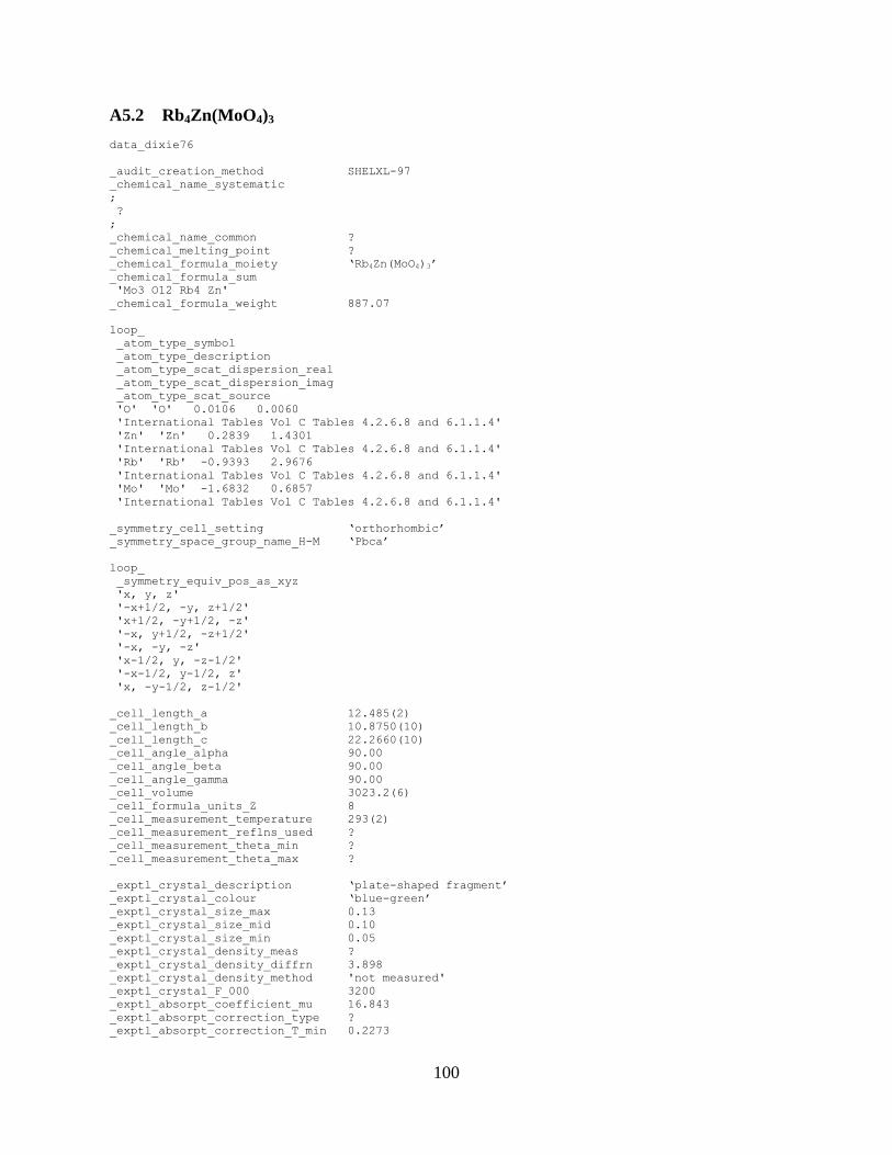
100
A5.2 Rb4Zn(MoO4)3
data_dixie76
_audit_creation_method SHELXL-97
_chemical_name_systematic
;
?
;
_chemical_name_common ?
_chemical_melting_point ?
_chemical_formula_moiety ‘Rb4Zn(MoO4)3’
_chemical_formula_sum
'Mo3 O12 Rb4 Zn'
_chemical_formula_weight 887.07
loop_
_atom_type_symbol
_atom_type_description
_atom_type_scat_dispersion_real
_atom_type_scat_dispersion_imag
_atom_type_scat_source
'O' 'O' 0.0106 0.0060
'International Tables Vol C Tables 4.2.6.8 and 6.1.1.4'
'Zn' 'Zn' 0.2839 1.4301
'International Tables Vol C Tables 4.2.6.8 and 6.1.1.4'
'Rb' 'Rb' -0.9393 2.9676
'International Tables Vol C Tables 4.2.6.8 and 6.1.1.4'
'Mo' 'Mo' -1.6832 0.6857
'International Tables Vol C Tables 4.2.6.8 and 6.1.1.4'
_symmetry_cell_setting ‘orthorhombic’
_symmetry_space_group_name_H-M ‘Pbca’
loop_
_symmetry_equiv_pos_as_xyz
'x, y, z'
'-x+1/2, -y, z+1/2'
'x+1/2, -y+1/2, -z'
'-x, y+1/2, -z+1/2'
'-x, -y, -z'
'x-1/2, y, -z-1/2'
'-x-1/2, y-1/2, z'
'x, -y-1/2, z-1/2'
_cell_length_a 12.485(2)
_cell_length_b 10.8750(10)
_cell_length_c 22.2660(10)
_cell_angle_alpha 90.00
_cell_angle_beta 90.00
_cell_angle_gamma 90.00
_cell_volume 3023.2(6)
_cell_formula_units_Z 8
_cell_measurement_temperature 293(2)
_cell_measurement_reflns_used ?
_cell_measurement_theta_min ?
_cell_measurement_theta_max ?
_exptl_crystal_description ‘plate-shaped fragment’
_exptl_crystal_colour ‘blue-green’
_exptl_crystal_size_max 0.13
_exptl_crystal_size_mid 0.10
_exptl_crystal_size_min 0.05
_exptl_crystal_density_meas ?
_exptl_crystal_density_diffrn 3.898
_exptl_crystal_density_method 'not measured'
_exptl_crystal_F_000 3200
_exptl_absorpt_coefficient_mu 16.843
_exptl_absorpt_correction_type ?
_exptl_absorpt_correction_T_min 0.2273

101
_exptl_absorpt_correction_T_max 0.4864
_exptl_absorpt_process_details ?
_exptl_special_details
;
?
;
_diffrn_ambient_temperature 293(2)
_diffrn_radiation_wavelength 0.71073
_diffrn_radiation_type MoK\a
_diffrn_radiation_source 'fine-focus sealed tube'
_diffrn_radiation_monochromator graphite
_diffrn_measurement_device_type 'KappaCCD'
_diffrn_measurement_method ' \w scans \k offsets'
_diffrn_detector_area_resol_mean ?
_diffrn_standards_number 0
_diffrn_standards_interval_count ?
_diffrn_standards_interval_time ?
_diffrn_standards_decay_% none
_diffrn_reflns_number 8235
_diffrn_reflns_av_R_equivalents 0.0535
_diffrn_reflns_av_sigmaI/netI 0.0624
_diffrn_reflns_limit_h_min -17
_diffrn_reflns_limit_h_max 17
_diffrn_reflns_limit_k_min -15
_diffrn_reflns_limit_k_max 15
_diffrn_reflns_limit_l_min -31
_diffrn_reflns_limit_l_max 31
_diffrn_reflns_theta_min 2.45
_diffrn_reflns_theta_max 30.02
_reflns_number_total 4419
_reflns_number_gt 2922
_reflns_threshold_expression >2sigma(I)
_computing_data_collection 'COLLECT (Nonius, 2000)'
_computing_cell_refinement 'Denzo and Scalepack (Otwinowski & Minor, 1997)'
_computing_data_reduction 'Denzo and Scalepack (Otwinowski & Minor, 1997)'
_computing_structure_solution 'SHELXS-97 (Sheldrick, 1990)'
_computing_structure_refinement 'SHELXL-97 (Sheldrick, 1997)'
_computing_molecular_graphics ?
_computing_publication_material 'SHELXL-97 (Sheldrick, 1997)'
_refine_special_details
;
Refinement of F^2^ against ALL reflections. The weighted R-factor wR and
goodness of fit S are based on F^2^, conventional R-factors R are based
on F, with F set to zero for negative F^2^. The threshold expression of
F^2^ > 2sigma(F^2^) is used only for calculating R-factors(gt) etc. and is
not relevant to the choice of reflections for refinement. R-factors based
on F^2^ are statistically about twice as large as those based on F, and R-
factors based on ALL data will be even larger.
;
_refine_ls_structure_factor_coef Fsqd
_refine_ls_matrix_type full
_refine_ls_weighting_scheme calc
_refine_ls_weighting_details
'calc w=1/[\s^2^(Fo^2^)+(0.0394P)^2^+9.0735P] where P=(Fo^2^+2Fc^2^)/3'
_atom_sites_solution_primary direct
_atom_sites_solution_secondary difmap
_atom_sites_solution_hydrogens geom
_refine_ls_hydrogen_treatment none
_refine_ls_extinction_method SHELXL
_refine_ls_extinction_coef 0.000134(18)
_refine_ls_extinction_expression
'Fc^*^=kFc[1+0.001xFc^2^\l^3^/sin(2\q)]^-1/4^'
_refine_ls_number_reflns 4419
_refine_ls_number_parameters 182
_refine_ls_number_restraints 0
_refine_ls_R_factor_all 0.0873
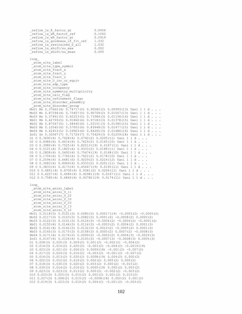
102
_refine_ls_R_factor_gt 0.0456
_refine_ls_wR_factor_ref 0.1062
_refine_ls_wR_factor_gt 0.0919
_refine_ls_goodness_of_fit_ref 1.032
_refine_ls_restrained_S_all 1.032
_refine_ls_shift/su_max 0.002
_refine_ls_shift/su_mean 0.000
loop_
_atom_site_label
_atom_site_type_symbol
_atom_site_fract_x
_atom_site_fract_y
_atom_site_fract_z
_atom_site_U_iso_or_equiv
_atom_site_adp_type
_atom_site_occupancy
_atom_site_symmetry_multiplicity
_atom_site_calc_flag
_atom_site_refinement_flags
_atom_site_disorder_assembly
_atom_site_disorder_group
Mo01 Mo 0.37662(4) 0.74717(5) 0.90582(2) 0.00993(13) Uani 1 1 d . . .
Mo02 Mo 0.87294(4) 0.75407(5) 0.90704(2) 0.01007(13) Uani 1 1 d . . .
Mo03 Mo 0.37491(5) 0.42223(5) 0.73384(3) 0.01156(14) Uani 1 1 d . . .
Rb01 Rb 0.62709(5) 0.91860(6) 0.97183(3) 0.01378(15) Uani 1 1 d . . .
Rb02 Rb 0.87567(5) 1.08440(6) 1.03151(3) 0.01385(15) Uani 1 1 d . . .
Rb03 Rb 0.10545(6) 0.57003(6) 0.83948(3) 0.01477(15) Uani 1 1 d . . .
Rb04 Rb 0.62453(5) 0.59903(6) 0.84265(3) 0.01486(16) Uani 1 1 d . . .
Zn01 Zn 0.32067(7) 0.71724(7) 0.75429(3) 0.01259(18) Uani 1 1 d . . .
O1 O 0.3690(4) 0.7428(4) 0.6740(2) 0.0205(11) Uani 1 1 d . . .
O2 O 0.4986(4) 0.4614(4) 0.7629(2) 0.0165(10) Uani 1 1 d . . .
O3 O 0.3980(4) 0.7525(4) 0.82513(19) 0.0167(11) Uani 1 1 d . . .
O4 O 0.5121(4) 0.1802(4) 0.9333(2) 0.0188(11) Uani 1 1 d . . .
O5 O 0.2808(4) 0.5400(4) 0.75474(19) 0.0168(10) Uani 1 1 d . . .
O6 O 0.1704(4) 0.7760(4) 0.7622(2) 0.0178(10) Uani 1 1 d . . .
O7 O 0.2594(4) 0.6681(5) 0.9229(2) 0.0224(12) Uani 1 1 d . . .
O8 O 0.3683(4) 0.8969(4) 0.9333(2) 0.0201(11) Uani 1 1 d . . .
O9 O 0.3833(4) 0.4173(4) 0.65647(19) 0.0195(11) Uani 1 1 d . . .
O10 O 0.4851(4) 0.6700(4) 0.9381(2) 0.0206(11) Uani 1 1 d . . .
O11 O 0.6227(4) 0.4084(4) 0.92981(19) 0.0167(11) Uani 1 1 d . . .
O12 O 0.7585(4) 0.6840(4) 0.93782(19) 0.0174(11) Uani 1 1 d . . .
loop_
_atom_site_aniso_label
_atom_site_aniso_U_11
_atom_site_aniso_U_22
_atom_site_aniso_U_33
_atom_site_aniso_U_23
_atom_site_aniso_U_13
_atom_site_aniso_U_12
Mo01 0.0118(3) 0.0101(3) 0.0080(3) 0.00017(19) -0.0003(2) -0.0005(2)
Mo02 0.0117(3) 0.0103(3) 0.0082(3) 0.0001(2) -0.0008(2) 0.0000(2)
Mo03 0.0122(3) 0.0101(3) 0.0124(3) -0.0004(2) -0.0004(2) -0.0001(2)
Rb01 0.0155(4) 0.0144(3) 0.0114(3) -0.0003(2) 0.0004(2) 0.0001(3)
Rb02 0.0141(4) 0.0142(3) 0.0132(3) 0.0010(2) -0.0005(2) 0.0001(3)
Rb03 0.0160(3) 0.0175(3) 0.0108(3) 0.0005(2) 0.0007(2) -0.0008(3)
Rb04 0.0171(4) 0.0176(3) 0.0099(3) -0.0003(2) 0.0004(3) -0.0029(3)
Zn01 0.0147(4) 0.0126(4) 0.0105(3) -0.0007(3) -0.0008(3) 0.0005(3)
O1 0.028(3) 0.025(3) 0.009(2) 0.001(2) -0.002(2) -0.004(2)
O2 0.014(3) 0.016(2) 0.020(2) -0.003(2) -0.004(2) -0.0019(19)
O3 0.023(3) 0.021(2) 0.006(2) 0.0009(18) -0.001(2) -0.007(2)
O4 0.017(3) 0.024(3) 0.016(2) -0.003(2) -0.001(2) -0.007(2)
O5 0.016(3) 0.013(2) 0.020(2) 0.0008(19) 0.004(2) 0.000(2)
O6 0.022(3) 0.012(2) 0.019(2) 0.002(2) 0.005(2) 0.000(2)
O7 0.018(3) 0.030(3) 0.020(2) 0.003(2) 0.000(2) -0.015(2)
O8 0.030(3) 0.014(2) 0.016(2) 0.0005(19) 0.005(2) 0.003(2)
O9 0.023(3) 0.023(3) 0.013(2) 0.000(2) -0.002(2) -0.003(2)
O10 0.022(3) 0.025(3) 0.015(2) 0.002(2) 0.001(2) 0.010(2)
O11 0.027(3) 0.008(2) 0.015(2) -0.0008(18) 0.002(2) 0.001(2)
O12 0.019(3) 0.023(3) 0.010(2) 0.004(2) -0.001(2) -0.003(2)
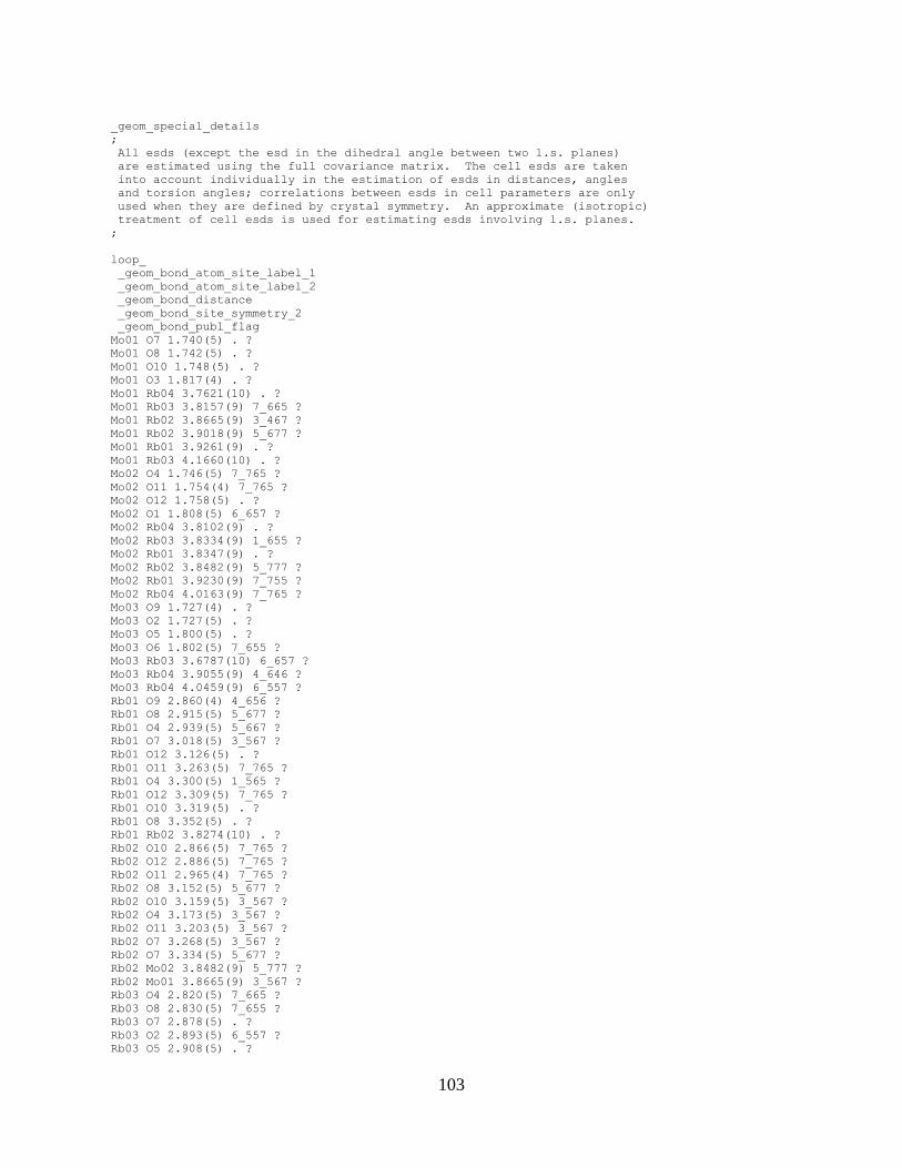
103
_geom_special_details
;
All esds (except the esd in the dihedral angle between two l.s. planes)
are estimated using the full covariance matrix. The cell esds are taken
into account individually in the estimation of esds in distances, angles
and torsion angles; correlations between esds in cell parameters are only
used when they are defined by crystal symmetry. An approximate (isotropic)
treatment of cell esds is used for estimating esds involving l.s. planes.
;
loop_
_geom_bond_atom_site_label_1
_geom_bond_atom_site_label_2
_geom_bond_distance
_geom_bond_site_symmetry_2
_geom_bond_publ_flag
Mo01 O7 1.740(5) . ?
Mo01 O8 1.742(5) . ?
Mo01 O10 1.748(5) . ?
Mo01 O3 1.817(4) . ?
Mo01 Rb04 3.7621(10) . ?
Mo01 Rb03 3.8157(9) 7_665 ?
Mo01 Rb02 3.8665(9) 3_467 ?
Mo01 Rb02 3.9018(9) 5_677 ?
Mo01 Rb01 3.9261(9) . ?
Mo01 Rb03 4.1660(10) . ?
Mo02 O4 1.746(5) 7_765 ?
Mo02 O11 1.754(4) 7_765 ?
Mo02 O12 1.758(5) . ?
Mo02 O1 1.808(5) 6_657 ?
Mo02 Rb04 3.8102(9) . ?
Mo02 Rb03 3.8334(9) 1_655 ?
Mo02 Rb01 3.8347(9) . ?
Mo02 Rb02 3.8482(9) 5_777 ?
Mo02 Rb01 3.9230(9) 7_755 ?
Mo02 Rb04 4.0163(9) 7_765 ?
Mo03 O9 1.727(4) . ?
Mo03 O2 1.727(5) . ?
Mo03 O5 1.800(5) . ?
Mo03 O6 1.802(5) 7_655 ?
Mo03 Rb03 3.6787(10) 6_657 ?
Mo03 Rb04 3.9055(9) 4_646 ?
Mo03 Rb04 4.0459(9) 6_557 ?
Rb01 O9 2.860(4) 4_656 ?
Rb01 O8 2.915(5) 5_677 ?
Rb01 O4 2.939(5) 5_667 ?
Rb01 O7 3.018(5) 3_567 ?
Rb01 O12 3.126(5) . ?
Rb01 O11 3.263(5) 7_765 ?
Rb01 O4 3.300(5) 1_565 ?
Rb01 O12 3.309(5) 7_765 ?
Rb01 O10 3.319(5) . ?
Rb01 O8 3.352(5) . ?
Rb01 Rb02 3.8274(10) . ?
Rb02 O10 2.866(5) 7_765 ?
Rb02 O12 2.886(5) 7_765 ?
Rb02 O11 2.965(4) 7_765 ?
Rb02 O8 3.152(5) 5_677 ?
Rb02 O10 3.159(5) 3_567 ?
Rb02 O4 3.173(5) 3_567 ?
Rb02 O11 3.203(5) 3_567 ?
Rb02 O7 3.268(5) 3_567 ?
Rb02 O7 3.334(5) 5_677 ?
Rb02 Mo02 3.8482(9) 5_777 ?
Rb02 Mo01 3.8665(9) 3_567 ?
Rb03 O4 2.820(5) 7_665 ?
Rb03 O8 2.830(5) 7_655 ?
Rb03 O7 2.878(5) . ?
Rb03 O2 2.893(5) 6_557 ?
Rb03 O5 2.908(5) . ?

104
Rb03 O6 2.939(4) . ?
Rb03 O9 3.234(5) 6_557 ?
Rb03 O3 3.468(5) 7_655 ?
Rb03 O1 3.512(5) 6_557 ?
Rb03 Zn01 3.6581(11) . ?
Rb03 Mo03 3.6787(10) 6_557 ?
Rb03 Mo01 3.8157(9) 7_655 ?
Rb04 O2 2.805(5) . ?
Rb04 O11 2.840(4) . ?
Rb04 O12 2.853(5) . ?
Rb04 O10 2.853(5) . ?
Rb04 O5 2.986(5) 6_657 ?
Rb04 O6 3.079(5) 6_657 ?
Rb04 O3 3.307(5) . ?
Rb04 O1 3.450(5) 6_657 ?
Rb04 O9 3.463(5) 4_656 ?
Rb04 Zn01 3.5083(11) 6_657 ?
Zn01 O3 1.889(5) . ?
Zn01 O1 1.908(5) . ?
Zn01 O6 1.990(5) . ?
Zn01 O5 1.991(5) . ?
Zn01 Rb04 3.5083(10) 6_557 ?
O1 Mo02 1.808(5) 6_557 ?
O1 Rb04 3.450(5) 6_557 ?
O1 Rb03 3.512(5) 6_657 ?
O2 Rb03 2.893(5) 6_657 ?
O3 Rb03 3.468(5) 7_665 ?
O4 Mo02 1.746(5) 7_755 ?
O4 Rb03 2.820(5) 7_655 ?
O4 Rb01 2.939(5) 5_667 ?
O4 Rb02 3.173(5) 3_467 ?
O4 Rb01 3.300(5) 1_545 ?
O5 Rb04 2.986(5) 6_557 ?
O6 Mo03 1.802(5) 7_665 ?
O6 Rb04 3.079(5) 6_557 ?
O7 Rb01 3.018(5) 3_467 ?
O7 Rb02 3.268(5) 3_467 ?
O7 Rb02 3.334(5) 5_677 ?
O8 Rb03 2.830(5) 7_665 ?
O8 Rb01 2.915(5) 5_677 ?
O8 Rb02 3.152(5) 5_677 ?
O9 Rb01 2.860(4) 4_646 ?
O9 Rb03 3.234(5) 6_657 ?
O9 Rb04 3.463(5) 4_646 ?
O10 Rb02 2.866(5) 7_755 ?
O10 Rb02 3.159(5) 3_467 ?
O11 Mo02 1.754(4) 7_755 ?
O11 Rb02 2.965(4) 7_755 ?
O11 Rb02 3.203(5) 3_467 ?
O11 Rb01 3.263(5) 7_755 ?
O12 Rb02 2.886(5) 7_755 ?
O12 Rb01 3.309(5) 7_755 ?
loop_
_geom_angle_atom_site_label_1
_geom_angle_atom_site_label_2
_geom_angle_atom_site_label_3
_geom_angle
_geom_angle_site_symmetry_1
_geom_angle_site_symmetry_3
_geom_angle_publ_flag
O7 Mo01 O8 109.6(2) . . ?
O7 Mo01 O10 109.0(2) . . ?
O8 Mo01 O10 110.5(2) . . ?
O7 Mo01 O3 110.9(2) . . ?
O8 Mo01 O3 109.0(2) . . ?
O10 Mo01 O3 107.9(2) . . ?
O7 Mo01 Rb04 124.23(18) . . ?
O8 Mo01 Rb04 125.49(17) . . ?
O10 Mo01 Rb04 46.42(15) . . ?
O3 Mo01 Rb04 61.52(16) . . ?
O7 Mo01 Rb03 126.07(18) . 7_665 ?
O8 Mo01 Rb03 43.88(15) . 7_665 ?
O10 Mo01 Rb03 123.74(17) . 7_665 ?
O3 Mo01 Rb03 65.11(15) . 7_665 ?
Rb04 Mo01 Rb03 101.60(2) . 7_665 ?
O7 Mo01 Rb02 57.15(18) . 3_467 ?
O8 Mo01 Rb02 138.15(15) . 3_467 ?
O10 Mo01 Rb02 53.58(17) . 3_467 ?
O3 Mo01 Rb02 112.78(15) . 3_467 ?
Rb04 Mo01 Rb02 74.818(18) . 3_467 ?
Rb03 Mo01 Rb02 176.41(2) 7_665 3_467 ?
O7 Mo01 Rb02 58.29(18) . 5_677 ?
O8 Mo01 Rb02 52.23(17) . 5_677 ?
O10 Mo01 Rb02 134.74(15) . 5_677 ?
O3 Mo01 Rb02 117.21(16) . 5_677 ?
Rb04 Mo01 Rb02 177.31(2) . 5_677 ?
Rb03 Mo01 Rb02 75.751(18) 7_665 5_677 ?
Rb02 Mo01 Rb02 107.831(18) 3_467 5_677 ?
O7 Mo01 Rb01 145.37(15) . . ?
O8 Mo01 Rb01 58.17(17) . . ?
O10 Mo01 Rb01 57.10(17) . . ?
O3 Mo01 Rb01 103.76(15) . . ?
Rb04 Mo01 Rb01 71.823(19) . . ?
Rb03 Mo01 Rb01 70.199(17) 7_665 . ?
Rb02 Mo01 Rb01 108.069(19) 3_467 . ?
Rb02 Mo01 Rb01 106.63(2) 5_677 . ?
O7 Mo01 Rb03 33.42(15) . . ?
O8 Mo01 Rb03 120.52(17) . . ?
O10 Mo01 Rb03 123.61(17) . . ?
O3 Mo01 Rb03 77.51(15) . . ?
Rb04 Mo01 Rb03 109.76(2) . . ?
Rb03 Mo01 Rb03 109.629(18) 7_665 . ?
Rb02 Mo01 Rb03 72.196(17) 3_467 . ?
Rb02 Mo01 Rb03 71.809(18) 5_677 . ?
Rb01 Mo01 Rb03 178.37(2) . . ?
O4 Mo02 O11 108.5(2) 7_765 7_765 ?
O4 Mo02 O12 109.8(2) 7_765 . ?
O11 Mo02 O12 109.1(2) 7_765 . ?
O4 Mo02 O1 109.0(2) 7_765 6_657 ?
O11 Mo02 O1 110.7(2) 7_765 6_657 ?
O12 Mo02 O1 109.7(2) . 6_657 ?
O4 Mo02 Rb04 126.29(16) 7_765 . ?
O11 Mo02 Rb04 123.88(16) 7_765 . ?
O12 Mo02 Rb04 45.04(14) . . ?
O1 Mo02 Rb04 64.70(16) 6_657 . ?
O4 Mo02 Rb03 42.99(15) 7_765 1_655 ?
O11 Mo02 Rb03 126.12(16) 7_765 1_655 ?
O12 Mo02 Rb03 122.84(16) . 1_655 ?
O1 Mo02 Rb03 66.03(16) 6_657 1_655 ?
Rb04 Mo02 Rb03 103.75(2) . 1_655 ?
O4 Mo02 Rb01 138.32(15) 7_765 . ?
O11 Mo02 Rb01 57.97(16) 7_765 . ?
O12 Mo02 Rb01 53.48(16) . . ?
O1 Mo02 Rb01 112.65(16) 6_657 . ?
Rb04 Mo02 Rb01 72.329(19) . . ?
Rb03 Mo02 Rb01 175.86(2) 1_655 . ?
O4 Mo02 Rb02 54.56(16) 7_765 5_777 ?
O11 Mo02 Rb02 55.61(16) 7_765 5_777 ?
O12 Mo02 Rb02 136.22(14) . 5_777 ?
O1 Mo02 Rb02 114.06(16) 6_657 5_777 ?
Rb04 Mo02 Rb02 178.56(2) . 5_777 ?
Rb03 Mo02 Rb02 76.13(2) 1_655 5_777 ?
Rb01 Mo02 Rb02 107.82(2) . 5_777 ?
O4 Mo02 Rb01 56.58(16) 7_765 7_755 ?
O11 Mo02 Rb01 141.58(14) 7_765 7_755 ?
O12 Mo02 Rb01 56.90(16) . 7_755 ?
O1 Mo02 Rb01 107.68(16) 6_657 7_755 ?
Rb04 Mo02 Rb01 74.145(17) . 7_755 ?
Rb03 Mo02 Rb01 70.053(17) 1_655 7_755 ?
Rb01 Mo02 Rb01 107.189(18) . 7_755 ?
Rb02 Mo02 Rb01 107.088(19) 5_777 7_755 ?

105
O4 Mo02 Rb04 122.87(17) 7_765 7_765 ?
O11 Mo02 Rb04 37.74(14) 7_765 7_765 ?
O12 Mo02 Rb04 123.37(16) . 7_765 ?
O1 Mo02 Rb04 72.99(16) 6_657 7_765 ?
Rb04 Mo02 Rb04 106.581(18) . 7_765 ?
Rb03 Mo02 Rb04 109.976(19) 1_655 7_765 ?
Rb01 Mo02 Rb04 72.826(17) . 7_765 ?
Rb02 Mo02 Rb04 72.190(16) 5_777 7_765 ?
Rb01 Mo02 Rb04 179.21(2) 7_755 7_765 ?
O9 Mo03 O2 109.1(2) . . ?
O9 Mo03 O5 108.6(2) . . ?
O2 Mo03 O5 108.2(2) . . ?
O9 Mo03 O6 109.9(2) . 7_655 ?
O2 Mo03 O6 111.5(2) . 7_655 ?
O5 Mo03 O6 109.4(2) . 7_655 ?
O9 Mo03 Rb03 61.53(16) . 6_657 ?
O2 Mo03 Rb03 50.14(15) . 6_657 ?
O5 Mo03 Rb03 108.36(15) . 6_657 ?
O6 Mo03 Rb03 141.88(16) 7_655 6_657 ?
O9 Mo03 Rb04 62.43(16) . 4_646 ?
O2 Mo03 Rb04 112.54(16) . 4_646 ?
O5 Mo03 Rb04 138.97(15) . 4_646 ?
O6 Mo03 Rb04 50.14(15) 7_655 4_646 ?
Rb03 Mo03 Rb04 101.439(19) 6_657 4_646 ?
O9 Mo03 Rb04 68.99(16) . 6_557 ?
O2 Mo03 Rb04 136.99(16) . 6_557 ?
O5 Mo03 Rb04 42.77(14) . 6_557 ?
O6 Mo03 Rb04 108.91(16) 7_655 6_557 ?
Rb03 Mo03 Rb04 102.13(2) 6_657 6_557 ?
Rb04 Mo03 Rb04 104.214(18) 4_646 6_557 ?
O9 Rb01 O8 136.77(14) 4_656 5_677 ?
O9 Rb01 O4 133.59(14) 4_656 5_667 ?
O8 Rb01 O4 75.06(13) 5_677 5_667 ?
O9 Rb01 O7 143.03(13) 4_656 3_567 ?
O8 Rb01 O7 68.97(13) 5_677 3_567 ?
O4 Rb01 O7 69.58(14) 5_667 3_567 ?
O9 Rb01 O12 77.16(12) 4_656 . ?
O8 Rb01 O12 136.63(13) 5_677 . ?
O4 Rb01 O12 100.71(13) 5_667 . ?
O7 Rb01 O12 69.26(12) 3_567 . ?
O9 Rb01 O11 75.92(13) 4_656 7_765 ?
O8 Rb01 O11 102.26(13) 5_677 7_765 ?
O4 Rb01 O11 139.43(12) 5_667 7_765 ?
O7 Rb01 O11 71.82(12) 3_567 7_765 ?
O12 Rb01 O11 53.16(12) . 7_765 ?
O9 Rb01 O4 74.03(12) 4_656 1_565 ?
O8 Rb01 O4 66.66(12) 5_677 1_565 ?
O4 Rb01 O4 104.17(11) 5_667 1_565 ?
O7 Rb01 O4 135.18(13) 3_567 1_565 ?
O12 Rb01 O4 150.32(11) . 1_565 ?
O11 Rb01 O4 111.80(11) 7_765 1_565 ?
O9 Rb01 O12 78.18(12) 4_656 7_765 ?
O8 Rb01 O12 63.70(12) 5_677 7_765 ?
O4 Rb01 O12 137.64(12) 5_667 7_765 ?
O7 Rb01 O12 102.36(13) 3_567 7_765 ?
O12 Rb01 O12 115.46(6) . 7_765 ?
O11 Rb01 O12 63.30(11) 7_765 7_765 ?
O4 Rb01 O12 51.42(12) 1_565 7_765 ?
O9 Rb01 O10 75.27(13) 4_656 . ?
O8 Rb01 O10 137.34(13) 5_677 . ?
O4 Rb01 O10 63.19(12) 5_667 . ?
O7 Rb01 O10 102.32(13) 3_567 . ?
O12 Rb01 O10 63.94(12) . . ?
O11 Rb01 O10 114.75(11) 7_765 . ?
O4 Rb01 O10 114.27(12) 1_565 . ?
O12 Rb01 O10 152.81(11) 7_765 . ?
O9 Rb01 O8 72.54(12) 4_656 . ?
O8 Rb01 O8 104.68(11) 5_677 . ?
O4 Rb01 O8 65.70(12) 5_667 . ?
O7 Rb01 O8 134.79(13) 3_567 . ?
O12 Rb01 O8 112.73(12) . . ?
O11 Rb01 O8 147.90(12) 7_765 . ?
O4 Rb01 O8 64.82(11) 1_565 . ?
O12 Rb01 O8 114.78(12) 7_765 . ?
O10 Rb01 O8 50.94(11) . . ?
O9 Rb01 Rb02 112.70(10) 4_656 . ?
O8 Rb01 Rb02 53.69(10) 5_677 . ?
O4 Rb01 Rb02 113.71(9) 5_667 . ?
O7 Rb01 Rb02 55.52(11) 3_567 . ?
O12 Rb01 Rb02 92.47(9) . . ?
O11 Rb01 Rb02 48.64(8) 7_765 . ?
O4 Rb01 Rb02 92.12(8) 1_565 . ?
O12 Rb01 Rb02 47.02(8) 7_765 . ?
O10 Rb01 Rb02 153.56(8) . . ?
O8 Rb01 Rb02 154.67(8) . . ?
O9 Rb01 Mo02 70.01(10) 4_656 . ?
O8 Rb01 Mo02 125.31(10) 5_677 . ?
O4 Rb01 Mo02 124.96(10) 5_667 . ?
O7 Rb01 Mo02 73.04(9) 3_567 . ?
O12 Rb01 Mo02 26.88(9) . . ?
O11 Rb01 Mo02 27.11(7) 7_765 . ?
O4 Rb01 Mo02 130.75(8) 1_565 . ?
O12 Rb01 Mo02 88.59(8) 7_765 . ?
O10 Rb01 Mo02 87.84(8) . . ?
O8 Rb01 Mo02 129.97(8) . . ?
Rb02 Rb01 Mo02 72.623(19) . . ?
O10 Rb02 O12 72.87(14) 7_765 7_765 ?
O10 Rb02 O11 69.59(13) 7_765 7_765 ?
O12 Rb02 O11 72.21(13) 7_765 7_765 ?
O10 Rb02 O8 138.23(13) 7_765 5_677 ?
O12 Rb02 O8 66.11(13) 7_765 5_677 ?
O11 Rb02 O8 103.79(13) 7_765 5_677 ?
O10 Rb02 O10 100.23(12) 7_765 3_567 ?
O12 Rb02 O10 137.28(13) 7_765 3_567 ?
O11 Rb02 O10 66.13(12) 7_765 3_567 ?
O8 Rb02 O10 114.91(12) 5_677 3_567 ?
O10 Rb02 O4 65.90(13) 7_765 3_567 ?
O12 Rb02 O4 100.78(13) 7_765 3_567 ?
O11 Rb02 O4 134.89(13) 7_765 3_567 ?
O8 Rb02 O4 113.90(12) 5_677 3_567 ?
O10 Rb02 O4 114.93(12) 3_567 3_567 ?
O10 Rb02 O11 66.63(13) 7_765 3_567 ?
O12 Rb02 O11 138.06(13) 7_765 3_567 ?
O11 Rb02 O11 102.39(11) 7_765 3_567 ?
O8 Rb02 O11 149.54(12) 5_677 3_567 ?
O10 Rb02 O11 63.08(12) 3_567 3_567 ?
O4 Rb02 O11 52.92(11) 3_567 3_567 ?
O10 Rb02 O7 140.15(13) 7_765 3_567 ?
O12 Rb02 O7 106.39(13) 7_765 3_567 ?
O11 Rb02 O7 72.40(12) 7_765 3_567 ?
O8 Rb02 O7 63.10(12) 5_677 3_567 ?
O10 Rb02 O7 52.39(13) 3_567 3_567 ?
O4 Rb02 O7 147.11(12) 3_567 3_567 ?
O11 Rb02 O7 111.40(12) 3_567 3_567 ?
O10 Rb02 O7 105.39(13) 7_765 5_677 ?
O12 Rb02 O7 67.88(12) 7_765 5_677 ?
O11 Rb02 O7 139.20(12) 7_765 5_677 ?
O8 Rb02 O7 51.93(12) 5_677 5_677 ?
O10 Rb02 O7 149.37(12) 3_567 5_677 ?
O4 Rb02 O7 62.94(12) 3_567 5_677 ?
O11 Rb02 O7 112.67(12) 3_567 5_677 ?
O7 Rb02 O7 111.05(7) 3_567 5_677 ?
O10 Rb02 Rb01 113.13(10) 7_765 . ?
O12 Rb02 Rb01 57.00(10) 7_765 . ?
O11 Rb02 Rb01 55.69(10) 7_765 . ?
O8 Rb02 Rb01 48.18(9) 5_677 . ?
O10 Rb02 Rb01 90.72(9) 3_567 . ?
O4 Rb02 Rb01 154.30(9) 3_567 . ?
O11 Rb02 Rb01 152.33(8) 3_567 . ?
O7 Rb02 Rb01 49.59(8) 3_567 . ?
O7 Rb02 Rb01 94.35(9) 5_677 . ?
O10 Rb02 Mo02 67.37(10) 7_765 5_777 ?

106
O12 Rb02 Mo02 123.98(10) 7_765 5_777 ?
O11 Rb02 Mo02 124.10(10) 7_765 5_777 ?
O8 Rb02 Mo02 132.08(9) 5_677 5_777 ?
O10 Rb02 Mo02 88.33(9) 3_567 5_777 ?
O4 Rb02 Mo02 26.64(9) 3_567 5_777 ?
O11 Rb02 Mo02 26.86(8) 3_567 5_777 ?
O7 Rb02 Mo02 129.46(9) 3_567 5_777 ?
O7 Rb02 Mo02 86.32(9) 5_677 5_777 ?
Rb01 Rb02 Mo02 179.00(2) . 5_777 ?
O10 Rb02 Mo01 124.27(10) 7_765 3_567 ?
O12 Rb02 Mo01 127.79(10) 7_765 3_567 ?
O11 Rb02 Mo01 70.95(8) 7_765 3_567 ?
O8 Rb02 Mo01 88.47(9) 5_677 3_567 ?
O10 Rb02 Mo01 26.44(9) 3_567 3_567 ?
O4 Rb02 Mo01 131.42(9) 3_567 3_567 ?
O11 Rb02 Mo01 85.57(8) 3_567 3_567 ?
O7 Rb02 Mo01 26.56(9) 3_567 3_567 ?
O7 Rb02 Mo01 130.13(8) 5_677 3_567 ?
Rb01 Rb02 Mo01 71.848(17) . 3_567 ?
Mo02 Rb02 Mo01 107.150(19) 5_777 3_567 ?
O4 Rb03 O8 78.26(14) 7_665 7_655 ?
O4 Rb03 O7 73.24(15) 7_665 . ?
O8 Rb03 O7 72.12(13) 7_655 . ?
O4 Rb03 O2 121.14(14) 7_665 6_557 ?
O8 Rb03 O2 111.27(13) 7_655 6_557 ?
O7 Rb03 O2 165.43(14) . 6_557 ?
O4 Rb03 O5 156.91(14) 7_665 . ?
O8 Rb03 O5 108.46(14) 7_655 . ?
O7 Rb03 O5 87.59(14) . . ?
O2 Rb03 O5 77.88(13) 6_557 . ?
O4 Rb03 O6 104.69(13) 7_665 . ?
O8 Rb03 O6 155.09(15) 7_655 . ?
O7 Rb03 O6 84.91(14) . . ?
O2 Rb03 O6 88.70(13) 6_557 . ?
O5 Rb03 O6 59.86(13) . . ?
O4 Rb03 O9 75.60(13) 7_665 6_557 ?
O8 Rb03 O9 74.77(13) 7_655 6_557 ?
O7 Rb03 O9 138.17(12) . 6_557 ?
O2 Rb03 O9 54.32(12) 6_557 6_557 ?
O5 Rb03 O9 127.29(12) . 6_557 ?
O6 Rb03 O9 130.12(13) . 6_557 ?
O4 Rb03 O3 119.00(13) 7_665 7_655 ?
O8 Rb03 O3 53.64(12) 7_655 7_655 ?
O7 Rb03 O3 115.90(13) . 7_655 ?
O2 Rb03 O3 60.99(12) 6_557 7_655 ?
O5 Rb03 O3 80.66(12) . 7_655 ?
O6 Rb03 O3 135.10(12) . 7_655 ?
O9 Rb03 O3 58.71(12) 6_557 7_655 ?
O4 Rb03 O1 53.02(12) 7_665 6_557 ?
O8 Rb03 O1 121.07(13) 7_655 6_557 ?
O7 Rb03 O1 114.70(14) . 6_557 ?
O2 Rb03 O1 76.34(12) 6_557 6_557 ?
O5 Rb03 O1 129.60(12) . 6_557 ?
O6 Rb03 O1 76.96(13) . 6_557 ?
O9 Rb03 O1 63.66(12) 6_557 6_557 ?
O3 Rb03 O1 120.96(12) 7_655 6_557 ?
O4 Rb03 Zn01 125.47(10) 7_665 . ?
O8 Rb03 Zn01 126.05(11) 7_655 . ?
O7 Rb03 Zn01 71.46(9) . . ?
O2 Rb03 Zn01 96.26(9) 6_557 . ?
O5 Rb03 Zn01 32.85(9) . . ?
O6 Rb03 Zn01 32.87(10) . . ?
O9 Rb03 Zn01 150.36(8) 6_557 . ?
O3 Rb03 Zn01 113.40(8) 7_655 . ?
O1 Rb03 Zn01 109.82(8) 6_557 . ?
O4 Rb03 Mo03 96.16(10) 7_665 6_557 ?
O8 Rb03 Mo03 97.32(10) 7_655 6_557 ?
O7 Rb03 Mo03 166.14(9) . 6_557 ?
O2 Rb03 Mo03 27.27(9) 6_557 6_557 ?
O5 Rb03 Mo03 104.59(9) . 6_557 ?
O6 Rb03 Mo03 106.80(10) . 6_557 ?
O9 Rb03 Mo03 27.99(8) 6_557 6_557 ?
O3 Rb03 Mo03 60.94(8) 7_655 6_557 ?
O1 Rb03 Mo03 62.51(8) 6_557 6_557 ?
Zn01 Rb03 Mo03 122.40(2) . 6_557 ?
O4 Rb03 Mo01 97.75(10) 7_665 7_655 ?
O8 Rb03 Mo01 25.26(9) 7_655 7_655 ?
O7 Rb03 Mo01 92.98(10) . 7_655 ?
O2 Rb03 Mo01 87.49(9) 6_557 7_655 ?
O5 Rb03 Mo01 95.95(9) . 7_655 ?
O6 Rb03 Mo01 155.76(10) . 7_655 ?
O9 Rb03 Mo01 64.34(9) 6_557 7_655 ?
O3 Rb03 Mo01 28.38(7) 7_655 7_655 ?
O1 Rb03 Mo01 125.07(8) 6_557 7_655 ?
Zn01 Rb03 Mo01 124.08(2) . 7_655 ?
Mo03 Rb03 Mo01 79.375(18) 6_557 7_655 ?
O2 Rb04 O11 92.21(13) . . ?
O2 Rb04 O12 166.33(13) . . ?
O11 Rb04 O12 74.55(13) . . ?
O2 Rb04 O10 105.90(14) . . ?
O11 Rb04 O10 71.55(13) . . ?
O12 Rb04 O10 73.54(14) . . ?
O2 Rb04 O5 77.97(13) . 6_657 ?
O11 Rb04 O5 110.15(13) . 6_657 ?
O12 Rb04 O5 103.07(13) . 6_657 ?
O10 Rb04 O5 175.83(14) . 6_657 ?
O2 Rb04 O6 87.60(12) . 6_657 ?
O11 Rb04 O6 167.39(13) . 6_657 ?
O12 Rb04 O6 104.56(13) . 6_657 ?
O10 Rb04 O6 120.60(13) . 6_657 ?
O5 Rb04 O6 57.49(13) 6_657 6_657 ?
O2 Rb04 O3 73.47(13) . . ?
O11 Rb04 O3 116.24(13) . . ?
O12 Rb04 O3 115.16(13) . . ?
O10 Rb04 O3 55.23(12) . . ?
O5 Rb04 O3 125.55(12) 6_657 . ?
O6 Rb04 O3 75.77(12) 6_657 . ?
O2 Rb04 O1 132.08(13) . 6_657 ?
O11 Rb04 O1 114.28(13) . 6_657 ?
O12 Rb04 O1 54.13(12) . 6_657 ?
O10 Rb04 O1 119.80(13) . 6_657 ?
O5 Rb04 O1 56.06(12) 6_657 6_657 ?
O6 Rb04 O1 58.05(12) 6_657 6_657 ?
O3 Rb04 O1 121.02(12) . 6_657 ?
O2 Rb04 O9 121.42(12) . 4_656 ?
O11 Rb04 O9 136.52(11) . 4_656 ?
O12 Rb04 O9 71.85(12) . 4_656 ?
O10 Rb04 O9 73.04(12) . 4_656 ?
O5 Rb04 O9 103.74(12) 6_657 4_656 ?
O6 Rb04 O9 52.02(11) 6_657 4_656 ?
O3 Rb04 O9 58.13(11) . 4_656 ?
O1 Rb04 O9 64.69(12) 6_657 4_656 ?
O2 Rb04 Zn01 101.38(10) . 6_657 ?
O11 Rb04 Zn01 133.91(10) . 6_657 ?
O12 Rb04 Zn01 85.93(10) . 6_657 ?
O10 Rb04 Zn01 141.71(10) . 6_657 ?
O5 Rb04 Zn01 34.53(9) 6_657 6_657 ?
O6 Rb04 Zn01 34.38(9) 6_657 6_657 ?
O3 Rb04 Zn01 109.84(8) . 6_657 ?
O1 Rb04 Zn01 31.82(8) 6_657 6_657 ?
O9 Rb04 Zn01 69.93(8) 4_656 6_657 ?
O2 Rb04 Mo01 90.23(10) . . ?
O11 Rb04 Mo01 92.89(9) . . ?
O12 Rb04 Mo01 93.77(10) . . ?
O10 Rb04 Mo01 26.35(9) . . ?
O5 Rb04 Mo01 154.27(9) 6_657 . ?
O6 Rb04 Mo01 99.72(9) 6_657 . ?
O3 Rb04 Mo01 28.88(8) . . ?
O1 Rb04 Mo01 125.03(9) 6_657 . ?
O9 Rb04 Mo01 63.04(8) 4_656 . ?
Zn01 Rb04 Mo01 130.34(3) 6_657 . ?
O2 Rb04 Mo02 158.55(10) . . ?

107
O11 Rb04 Mo02 94.15(10) . . ?
O12 Rb04 Mo02 25.86(9) . . ?
O10 Rb04 Mo02 95.54(10) . . ?
O5 Rb04 Mo02 80.60(9) 6_657 . ?
O6 Rb04 Mo02 81.79(9) 6_657 . ?
O3 Rb04 Mo02 121.14(8) . . ?
O1 Rb04 Mo02 28.29(8) 6_657 . ?
O9 Rb04 Mo02 65.07(8) 4_656 . ?
Zn01 Rb04 Mo02 60.078(19) 6_657 . ?
Mo01 Rb04 Mo02 109.85(2) . . ?
O3 Zn01 O1 126.3(2) . . ?
O3 Zn01 O6 110.1(2) . . ?
O1 Zn01 O6 109.5(2) . . ?
O3 Zn01 O5 108.69(19) . . ?
O1 Zn01 O5 103.00(19) . . ?
O6 Zn01 O5 94.28(19) . . ?
O3 Zn01 Rb04 160.92(15) . 6_557 ?
O1 Zn01 Rb04 72.39(15) . 6_557 ?
O6 Zn01 Rb04 60.91(14) . 6_557 ?
O5 Zn01 Rb04 58.24(13) . 6_557 ?
O3 Zn01 Rb03 91.80(14) . . ?
O1 Zn01 Rb03 141.46(15) . . ?
O6 Zn01 Rb03 53.29(13) . . ?
O5 Zn01 Rb03 52.40(13) . . ?
Rb04 Zn01 Rb03 69.26(2) 6_557 . ?
Mo02 O1 Zn01 162.4(3) 6_557 . ?
Mo02 O1 Rb04 87.01(17) 6_557 6_557 ?
Zn01 O1 Rb04 75.78(15) . 6_557 ?
Mo02 O1 Rb03 85.90(17) 6_557 6_657 ?
Zn01 O1 Rb03 105.53(19) . 6_657 ?
Rb04 O1 Rb03 119.48(14) 6_557 6_657 ?
Mo03 O2 Rb04 150.4(2) . . ?
Mo03 O2 Rb03 102.59(19) . 6_657 ?
Rb04 O2 Rb03 91.27(13) . 6_657 ?
Mo01 O3 Zn01 138.1(3) . . ?
Mo01 O3 Rb04 89.60(17) . . ?
Zn01 O3 Rb04 115.7(2) . . ?
Mo01 O3 Rb03 86.51(16) . 7_665 ?
Zn01 O3 Rb03 105.83(18) . 7_665 ?
Rb04 O3 Rb03 120.16(14) . 7_665 ?
Mo02 O4 Rb03 112.0(2) 7_755 7_655 ?
Mo02 O4 Rb01 153.5(2) 7_755 5_667 ?
Rb03 O4 Rb01 93.99(14) 7_655 5_667 ?
Mo02 O4 Rb02 98.80(19) 7_755 3_467 ?
Rb03 O4 Rb02 104.28(15) 7_655 3_467 ?
Rb01 O4 Rb02 78.48(12) 5_667 3_467 ?
Mo02 O4 Rb01 97.2(2) 7_755 1_545 ?
Rb03 O4 Rb01 93.01(13) 7_655 1_545 ?
Rb01 O4 Rb01 75.83(11) 5_667 1_545 ?
Rb02 O4 Rb01 149.86(16) 3_467 1_545 ?
Mo03 O5 Zn01 121.6(3) . . ?
Mo03 O5 Rb03 137.7(2) . . ?
Zn01 O5 Rb03 94.75(17) . . ?
Mo03 O5 Rb04 113.07(19) . 6_557 ?
Zn01 O5 Rb04 87.23(16) . 6_557 ?
Rb03 O5 Rb04 87.44(13) . 6_557 ?
Mo03 O6 Zn01 123.3(2) 7_665 . ?
Mo03 O6 Rb03 142.3(2) 7_665 . ?
Zn01 O6 Rb03 93.84(16) . . ?
Mo03 O6 Rb04 103.17(19) 7_665 6_557 ?
Zn01 O6 Rb04 84.71(15) . 6_557 ?
Rb03 O6 Rb04 85.19(12) . 6_557 ?
Mo01 O7 Rb03 127.1(2) . . ?
Mo01 O7 Rb01 141.7(2) . 3_467 ?
Rb03 O7 Rb01 91.14(13) . 3_467 ?
Mo01 O7 Rb02 96.3(2) . 3_467 ?
Rb03 O7 Rb02 100.70(14) . 3_467 ?
Rb01 O7 Rb02 74.89(11) 3_467 3_467 ?
Mo01 O7 Rb02 95.4(2) . 5_677 ?
Rb03 O7 Rb02 99.09(15) . 5_677 ?
Rb01 O7 Rb02 74.88(11) 3_467 5_677 ?
Rb02 O7 Rb02 143.95(15) 3_467 5_677 ?
Mo01 O8 Rb03 110.9(2) . 7_665 ?
Mo01 O8 Rb01 153.7(2) . 5_677 ?
Rb03 O8 Rb01 94.29(14) 7_665 5_677 ?
Mo01 O8 Rb02 101.9(2) . 5_677 ?
Rb03 O8 Rb02 104.64(15) 7_665 5_677 ?
Rb01 O8 Rb02 78.13(11) 5_677 5_677 ?
Mo01 O8 Rb01 95.62(19) . . ?
Rb03 O8 Rb01 91.75(13) 7_665 . ?
Rb01 O8 Rb01 75.32(11) 5_677 . ?
Rb02 O8 Rb01 149.69(15) 5_677 . ?
Mo03 O9 Rb01 173.6(3) . 4_646 ?
Mo03 O9 Rb03 90.48(18) . 6_657 ?
Rb01 O9 Rb03 93.68(13) 4_646 6_657 ?
Mo03 O9 Rb04 91.35(18) . 4_646 ?
Rb01 O9 Rb04 90.53(12) 4_646 4_646 ?
Rb03 O9 Rb04 122.50(15) 6_657 4_646 ?
Mo01 O10 Rb04 107.2(2) . . ?
Mo01 O10 Rb02 157.6(2) . 7_755 ?
Rb04 O10 Rb02 94.75(14) . 7_755 ?
Mo01 O10 Rb02 100.0(2) . 3_467 ?
Rb04 O10 Rb02 100.75(14) . 3_467 ?
Rb02 O10 Rb02 79.77(12) 7_755 3_467 ?
Mo01 O10 Rb01 96.65(19) . . ?
Rb04 O10 Rb01 93.62(14) . . ?
Rb02 O10 Rb01 77.09(12) 7_755 . ?
Rb02 O10 Rb01 153.63(16) 3_467 . ?
Mo02 O11 Rb04 120.0(2) 7_755 . ?
Mo02 O11 Rb02 147.0(2) 7_755 7_755 ?
Rb04 O11 Rb02 92.90(12) . 7_755 ?
Mo02 O11 Rb02 97.53(18) 7_755 3_467 ?
Rb04 O11 Rb02 100.00(14) . 3_467 ?
Rb02 O11 Rb02 77.61(11) 7_755 3_467 ?
Mo02 O11 Rb01 94.92(18) 7_755 7_755 ?
Rb04 O11 Rb01 99.40(13) . 7_755 ?
Rb02 O11 Rb01 75.67(10) 7_755 7_755 ?
Rb02 O11 Rb01 147.56(15) 3_467 7_755 ?
Mo02 O12 Rb04 109.10(19) . . ?
Mo02 O12 Rb02 156.3(2) . 7_755 ?
Rb04 O12 Rb02 94.30(14) . 7_755 ?
Mo02 O12 Rb01 99.64(19) . . ?
Rb04 O12 Rb01 97.86(14) . . ?
Rb02 O12 Rb01 80.02(12) 7_755 . ?
Mo02 O12 Rb01 96.66(19) . 7_755 ?
Rb04 O12 Rb01 98.07(13) . 7_755 ?
Rb02 O12 Rb01 75.97(10) 7_755 7_755 ?
Rb01 O12 Rb01 152.02(15) . 7_755 ?
_diffrn_measured_fraction_theta_max 1.000
_diffrn_reflns_theta_full 30.02
_diffrn_measured_fraction_theta_full 1.000
_refine_diff_density_max 2.495
_refine_diff_density_min -1.940
_refine_diff_density_rms 0.317
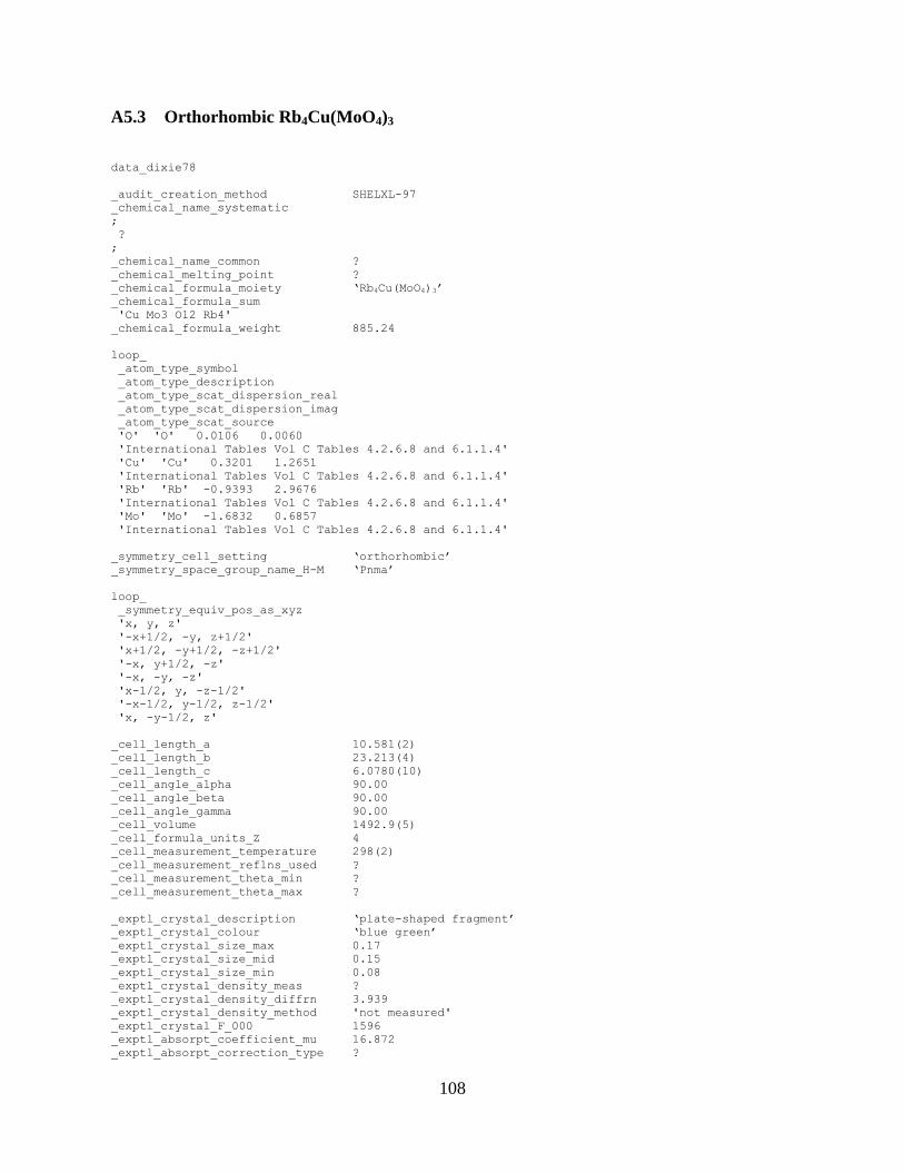
108
A5.3 Orthorhombic Rb4Cu(MoO4)3
data_dixie78
_audit_creation_method SHELXL-97
_chemical_name_systematic
;
?
;
_chemical_name_common ?
_chemical_melting_point ?
_chemical_formula_moiety ‘Rb4Cu(MoO4)3’
_chemical_formula_sum
'Cu Mo3 O12 Rb4'
_chemical_formula_weight 885.24
loop_
_atom_type_symbol
_atom_type_description
_atom_type_scat_dispersion_real
_atom_type_scat_dispersion_imag
_atom_type_scat_source
'O' 'O' 0.0106 0.0060
'International Tables Vol C Tables 4.2.6.8 and 6.1.1.4'
'Cu' 'Cu' 0.3201 1.2651
'International Tables Vol C Tables 4.2.6.8 and 6.1.1.4'
'Rb' 'Rb' -0.9393 2.9676
'International Tables Vol C Tables 4.2.6.8 and 6.1.1.4'
'Mo' 'Mo' -1.6832 0.6857
'International Tables Vol C Tables 4.2.6.8 and 6.1.1.4'
_symmetry_cell_setting ‘orthorhombic’
_symmetry_space_group_name_H-M ‘Pnma’
loop_
_symmetry_equiv_pos_as_xyz
'x, y, z'
'-x+1/2, -y, z+1/2'
'x+1/2, -y+1/2, -z+1/2'
'-x, y+1/2, -z'
'-x, -y, -z'
'x-1/2, y, -z-1/2'
'-x-1/2, y-1/2, z-1/2'
'x, -y-1/2, z'
_cell_length_a 10.581(2)
_cell_length_b 23.213(4)
_cell_length_c 6.0780(10)
_cell_angle_alpha 90.00
_cell_angle_beta 90.00
_cell_angle_gamma 90.00
_cell_volume 1492.9(5)
_cell_formula_units_Z 4
_cell_measurement_temperature 298(2)
_cell_measurement_reflns_used ?
_cell_measurement_theta_min ?
_cell_measurement_theta_max ?
_exptl_crystal_description ‘plate-shaped fragment’
_exptl_crystal_colour ‘blue green’
_exptl_crystal_size_max 0.17
_exptl_crystal_size_mid 0.15
_exptl_crystal_size_min 0.08
_exptl_crystal_density_meas ?
_exptl_crystal_density_diffrn 3.939
_exptl_crystal_density_method 'not measured'
_exptl_crystal_F_000 1596
_exptl_absorpt_coefficient_mu 16.872
_exptl_absorpt_correction_type ?

109
_exptl_absorpt_correction_T_min 0.1562
_exptl_absorpt_correction_T_max 0.3643
_exptl_absorpt_process_details ?
_exptl_special_details
;
?
;
_diffrn_ambient_temperature 298(2)
_diffrn_radiation_wavelength 0.71073
_diffrn_radiation_type MoK\a
_diffrn_radiation_source 'fine-focus sealed tube'
_diffrn_radiation_monochromator graphite
_diffrn_measurement_device_type 'KappaCCD'
_diffrn_measurement_method ' \w scans \k offsets'
_diffrn_detector_area_resol_mean ?
_diffrn_standards_number 0
_diffrn_standards_interval_count ?
_diffrn_standards_interval_time ?
_diffrn_standards_decay_% none
_diffrn_reflns_number 3948
_diffrn_reflns_av_R_equivalents 0.0295
_diffrn_reflns_av_sigmaI/netI 0.0401
_diffrn_reflns_limit_h_min -14
_diffrn_reflns_limit_h_max 14
_diffrn_reflns_limit_k_min -32
_diffrn_reflns_limit_k_max 32
_diffrn_reflns_limit_l_min -8
_diffrn_reflns_limit_l_max 8
_diffrn_reflns_theta_min 3.46
_diffrn_reflns_theta_max 30.02
_reflns_number_total 2222
_reflns_number_gt 1582
_reflns_threshold_expression >2sigma(I)
_computing_data_collection 'COLLECT (Nonius, 2000)'
_computing_cell_refinement 'Denzo and Scalepack (Otwinowski & Minor, 1997)'
_computing_data_reduction 'Denzo and Scalepack (Otwinowski & Minor, 1997)'
_computing_structure_solution 'SHELXS-97 (Sheldrick, 1990)'
_computing_structure_refinement 'SHELXL-97 (Sheldrick, 1997)'
_computing_molecular_graphics ?
_computing_publication_material 'SHELXL-97 (Sheldrick, 1997)'
_refine_special_details
;
Refinement of F^2^ against ALL reflections. The weighted R-factor wR and
goodness of fit S are based on F^2^, conventional R-factors R are based
on F, with F set to zero for negative F^2^. The threshold expression of
F^2^ > 2sigma(F^2^) is used only for calculating R-factors(gt) etc. and is
not relevant to the choice of reflections for refinement. R-factors based
on F^2^ are statistically about twice as large as those based on F, and R-
factors based on ALL data will be even larger.
;
_refine_ls_structure_factor_coef Fsqd
_refine_ls_matrix_type full
_refine_ls_weighting_scheme calc
_refine_ls_weighting_details
'calc w=1/[\s^2^(Fo^2^)+(0.0207P)^2^+31.5979P] where P=(Fo^2^+2Fc^2^)/3'
_atom_sites_solution_primary direct
_atom_sites_solution_secondary difmap
_atom_sites_solution_hydrogens geom
_refine_ls_hydrogen_treatment none
_refine_ls_extinction_method SHELXL
_refine_ls_extinction_coef 0.00084(11)
_refine_ls_extinction_expression
'Fc^*^=kFc[1+0.001xFc^2^\l^3^/sin(2\q)]^-1/4^'
_refine_ls_number_reflns 2222
_refine_ls_number_parameters 107
_refine_ls_number_restraints 0
_refine_ls_R_factor_all 0.0729
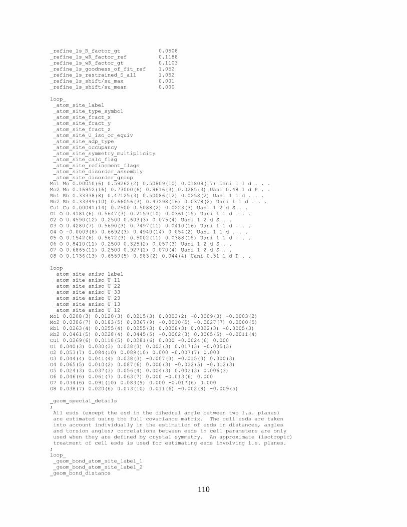
110
_refine_ls_R_factor_gt 0.0508
_refine_ls_wR_factor_ref 0.1188
_refine_ls_wR_factor_gt 0.1103
_refine_ls_goodness_of_fit_ref 1.052
_refine_ls_restrained_S_all 1.052
_refine_ls_shift/su_max 0.001
_refine_ls_shift/su_mean 0.000
loop_
_atom_site_label
_atom_site_type_symbol
_atom_site_fract_x
_atom_site_fract_y
_atom_site_fract_z
_atom_site_U_iso_or_equiv
_atom_site_adp_type
_atom_site_occupancy
_atom_site_symmetry_multiplicity
_atom_site_calc_flag
_atom_site_refinement_flags
_atom_site_disorder_assembly
_atom_site_disorder_group
Mo1 Mo 0.00050(6) 0.59262(2) 0.50809(10) 0.01809(17) Uani 1 1 d . . .
Mo2 Mo 0.16952(16) 0.73000(6) 0.9616(3) 0.0285(3) Uani 0.48 1 d P . .
Rb1 Rb 0.33338(8) 0.47125(3) 0.50086(12) 0.0258(2) Uani 1 1 d . . .
Rb2 Rb 0.33349(10) 0.66056(3) 0.47298(16) 0.0378(2) Uani 1 1 d . . .
Cu1 Cu 0.00041(14) 0.2500 0.5088(2) 0.0223(3) Uani 1 2 d S . .
O1 O 0.4181(6) 0.5647(3) 0.2159(10) 0.0361(15) Uani 1 1 d . . .
O2 O 0.4590(12) 0.2500 0.603(3) 0.075(4) Uani 1 2 d S . .
O3 O 0.4280(7) 0.5690(3) 0.7497(11) 0.0410(16) Uani 1 1 d . . .
O4 O -0.0003(8) 0.6692(3) 0.4940(14) 0.054(2) Uani 1 1 d . . .
O5 O 0.1542(6) 0.5672(3) 0.5002(11) 0.0388(15) Uani 1 1 d . . .
O6 O 0.8410(11) 0.2500 0.325(2) 0.057(3) Uani 1 2 d S . .
O7 O 0.6865(11) 0.2500 0.927(2) 0.070(4) Uani 1 2 d S . .
O8 O 0.1736(13) 0.6559(5) 0.983(2) 0.044(4) Uani 0.51 1 d P . .
loop_
_atom_site_aniso_label
_atom_site_aniso_U_11
_atom_site_aniso_U_22
_atom_site_aniso_U_33
_atom_site_aniso_U_23
_atom_site_aniso_U_13
_atom_site_aniso_U_12
Mo1 0.0208(3) 0.0120(3) 0.0215(3) 0.0003(2) -0.0009(3) -0.0003(2)
Mo2 0.0306(7) 0.0183(5) 0.0367(9) -0.0010(5) -0.0027(7) 0.0000(5)
Rb1 0.0263(4) 0.0255(4) 0.0255(3) 0.0008(3) 0.0022(3) -0.0005(3)
Rb2 0.0461(5) 0.0228(4) 0.0445(5) -0.0002(3) 0.0065(5) -0.0011(4)
Cu1 0.0269(6) 0.0118(5) 0.0281(6) 0.000 -0.0024(6) 0.000
O1 0.040(3) 0.030(3) 0.038(3) 0.003(3) 0.017(3) -0.005(3)
O2 0.053(7) 0.084(10) 0.089(10) 0.000 -0.007(7) 0.000
O3 0.044(4) 0.041(4) 0.038(3) -0.007(3) -0.015(3) 0.000(3)
O4 0.065(5) 0.010(2) 0.087(6) 0.000(3) -0.022(5) -0.012(3)
O5 0.024(3) 0.037(3) 0.056(4) 0.004(3) 0.002(3) 0.006(3)
O6 0.046(6) 0.061(7) 0.063(7) 0.000 -0.013(6) 0.000
O7 0.034(6) 0.091(10) 0.083(9) 0.000 -0.017(6) 0.000
O8 0.038(7) 0.020(6) 0.073(10) 0.011(6) -0.002(8) -0.009(5)
_geom_special_details
;
All esds (except the esd in the dihedral angle between two l.s. planes)
are estimated using the full covariance matrix. The cell esds are taken
into account individually in the estimation of esds in distances, angles
and torsion angles; correlations between esds in cell parameters are only
used when they are defined by crystal symmetry. An approximate (isotropic)
treatment of cell esds is used for estimating esds involving l.s. planes.
;
loop_
_geom_bond_atom_site_label_1
_geom_bond_atom_site_label_2
_geom_bond_distance

111
_geom_bond_site_symmetry_2
_geom_bond_publ_flag
Mo1 O5 1.731(6) . ?
Mo1 O1 1.741(6) 6_556 ?
Mo1 O3 1.748(6) 6_557 ?
Mo1 O4 1.780(6) . ?
Mo1 Rb2 3.7629(12) 6_556 ?
Mo1 Rb1 3.7759(11) 2_565 ?
Mo1 Rb1 3.8316(12) 5_566 ?
Mo1 Rb1 3.8460(11) 2_564 ?
Mo1 Rb2 3.8661(14) . ?
Mo1 Rb2 3.9443(13) 6_557 ?
Mo2 Mo2 0.929(3) 8_575 ?
Mo2 O2 1.674(13) 2_565 ?
Mo2 O8 1.726(11) . ?
Mo2 O7 1.730(11) 5_667 ?
Mo2 O6 1.805(12) 5_666 ?
Mo2 Rb2 3.798(2) . ?
Mo2 Rb2 3.908(2) 1_556 ?
Mo2 Rb2 3.924(2) 6_557 ?
Mo2 Rb2 4.2761(19) 8_575 ?
Rb1 O3 2.905(6) . ?
Rb1 O1 2.918(6) . ?
Rb1 O5 2.926(6) . ?
Rb1 O8 2.954(11) 2_564 ?
Rb1 O1 3.080(7) 2_565 ?
Rb1 O3 3.093(7) 5_666 ?
Rb1 O5 3.166(7) 2_565 ?
Rb1 O5 3.174(7) 2_564 ?
Rb1 O1 3.252(7) 5_666 ?
Rb1 O3 3.294(7) 2_564 ?
Rb1 Rb1 3.7591(10) 2_565 ?
Rb1 Rb1 3.7591(10) 2_564 ?
Rb2 O1 2.862(6) . ?
Rb2 O5 2.884(7) . ?
Rb2 O3 2.889(7) . ?
Rb2 O6 3.038(9) 5_666 ?
Rb2 O2 3.057(10) 5_666 ?
Rb2 O7 3.205(11) 5_666 ?
Rb2 O4 3.345(8) 6_656 ?
Rb2 O8 3.425(15) 1_554 ?
Rb2 O8 3.535(15) . ?
Rb2 O4 3.540(9) . ?
Rb2 O8 3.610(14) 6_657 ?
Rb2 Mo1 3.7629(12) 6_656 ?
Cu1 O4 1.876(6) 4_546 ?
Cu1 O4 1.876(6) 5_566 ?
Cu1 O7 2.007(12) 6_557 ?
Cu1 O6 2.023(11) 1_455 ?
Cu1 O2 2.400(15) 6_557 ?
Cu1 Rb2 3.9191(15) 2_565 ?
Cu1 Rb2 3.9191(15) 7_656 ?
Cu1 Rb2 4.0994(17) 4_546 ?
Cu1 Rb2 4.0994(17) 5_566 ?
Cu1 Rb2 4.2433(16) 7_655 ?
Cu1 Rb2 4.2433(16) 2_564 ?
O1 Mo1 1.741(6) 6_656 ?
O1 Rb1 3.080(7) 2_564 ?
O1 Rb1 3.252(7) 5_666 ?
O2 Mo2 1.674(13) 7_655 ?
O2 Mo2 1.674(13) 2_564 ?
O2 Cu1 2.400(15) 6_657 ?
O2 Rb2 3.057(10) 5_666 ?
O2 Rb2 3.057(10) 4_646 ?
O3 Mo1 1.748(6) 6_657 ?
O3 Rb1 3.093(7) 5_666 ?
O3 Rb1 3.294(7) 2_565 ?
O4 Cu1 1.876(6) 5_566 ?
O4 Rb2 3.345(8) 6_556 ?
O5 Rb1 3.166(7) 2_564 ?
O5 Rb1 3.174(7) 2_565 ?
O6 Mo2 1.805(12) 4_646 ?
O6 Mo2 1.805(12) 5_666 ?
O6 Cu1 2.023(11) 1_655 ?
O6 Rb2 3.038(9) 4_646 ?
O6 Rb2 3.038(9) 5_666 ?
O7 Mo2 1.730(11) 5_667 ?
O7 Mo2 1.730(11) 4_647 ?
O7 Cu1 2.007(12) 6_657 ?
O7 Rb2 3.205(11) 4_646 ?
O7 Rb2 3.205(11) 5_666 ?
O8 Rb1 2.954(11) 2_565 ?
O8 Rb2 3.425(15) 1_556 ?
O8 Rb2 3.610(14) 6_557 ?
loop_
_geom_angle_atom_site_label_1
_geom_angle_atom_site_label_2
_geom_angle_atom_site_label_3
_geom_angle
_geom_angle_site_symmetry_1
_geom_angle_site_symmetry_3
_geom_angle_publ_flag
O5 Mo1 O1 108.8(3) . 6_556 ?
O5 Mo1 O3 109.2(3) . 6_557 ?
O1 Mo1 O3 108.8(3) 6_556 6_557 ?
O5 Mo1 O4 110.1(4) . . ?
O1 Mo1 O4 109.3(3) 6_556 . ?
O3 Mo1 O4 110.6(4) 6_557 . ?
O5 Mo1 Rb2 124.2(2) . 6_556 ?
O1 Mo1 Rb2 46.6(2) 6_556 6_556 ?
O3 Mo1 Rb2 125.4(2) 6_557 6_556 ?
O4 Mo1 Rb2 62.7(3) . 6_556 ?
O5 Mo1 Rb1 56.7(2) . 2_565 ?
O1 Mo1 Rb1 135.0(2) 6_556 2_565 ?
O3 Mo1 Rb1 54.1(2) 6_557 2_565 ?
O4 Mo1 Rb1 115.6(3) . 2_565 ?
Rb2 Mo1 Rb1 178.21(2) 6_556 2_565 ?
O5 Mo1 Rb1 137.3(2) . 5_566 ?
O1 Mo1 Rb1 51.9(2) 6_556 5_566 ?
O3 Mo1 Rb1 59.1(2) 6_557 5_566 ?
O4 Mo1 Rb1 112.4(3) . 5_566 ?
Rb2 Mo1 Rb1 73.63(2) 6_556 5_566 ?
Rb1 Mo1 Rb1 106.77(2) 2_565 5_566 ?
O5 Mo1 Rb1 54.3(2) . 2_564 ?
O1 Mo1 Rb1 57.2(2) 6_556 2_564 ?
O3 Mo1 Rb1 139.0(2) 6_557 2_564 ?
O4 Mo1 Rb1 110.4(3) . 2_564 ?
Rb2 Mo1 Rb1 75.72(3) 6_556 2_564 ?
Rb1 Mo1 Rb1 105.77(3) 2_565 2_564 ?
Rb1 Mo1 Rb1 105.12(2) 5_566 2_564 ?
O5 Mo1 Rb2 44.0(2) . . ?
O1 Mo1 Rb2 124.4(2) 6_556 . ?
O3 Mo1 Rb2 125.0(2) 6_557 . ?
O4 Mo1 Rb2 66.1(3) . . ?
Rb2 Mo1 Rb2 102.36(2) 6_556 . ?
Rb1 Mo1 Rb2 77.27(2) 2_565 . ?
Rb1 Mo1 Rb2 175.80(3) 5_566 . ?
Rb1 Mo1 Rb2 72.33(2) 2_564 . ?
O5 Mo1 Rb2 125.4(2) . 6_557 ?
O1 Mo1 Rb2 123.3(2) 6_556 6_557 ?
O3 Mo1 Rb2 41.9(2) 6_557 6_557 ?
O4 Mo1 Rb2 68.7(3) . 6_557 ?
Rb2 Mo1 Rb2 104.09(3) 6_556 6_557 ?
Rb1 Mo1 Rb2 74.41(2) 2_565 6_557 ?
Rb1 Mo1 Rb2 75.70(2) 5_566 6_557 ?
Rb1 Mo1 Rb2 179.02(2) 2_564 6_557 ?
Rb2 Mo1 Rb2 106.82(2) . 6_557 ?
Mo2 Mo2 O2 73.89(14) 8_575 2_565 ?
Mo2 Mo2 O8 175.4(5) 8_575 . ?
O2 Mo2 O8 104.9(5) 2_565 . ?
Mo2 Mo2 O7 74.43(12) 8_575 5_667 ?

112
O2 Mo2 O7 116.1(6) 2_565 5_667 ?
O8 Mo2 O7 102.5(5) . 5_667 ?
Mo2 Mo2 O6 75.10(11) 8_575 5_666 ?
O2 Mo2 O6 111.9(6) 2_565 5_666 ?
O8 Mo2 O6 109.4(5) . 5_666 ?
O7 Mo2 O6 111.2(6) 5_667 5_666 ?
Mo2 Mo2 Rb2 115.11(3) 8_575 . ?
O2 Mo2 Rb2 152.9(5) 2_565 . ?
O8 Mo2 Rb2 68.0(5) . . ?
O7 Mo2 Rb2 91.0(4) 5_667 . ?
O6 Mo2 Rb2 51.9(3) 5_666 . ?
Mo2 Mo2 Rb2 114.36(3) 8_575 1_556 ?
O2 Mo2 Rb2 93.8(5) 2_565 1_556 ?
O8 Mo2 Rb2 61.1(5) . 1_556 ?
O7 Mo2 Rb2 53.8(3) 5_667 1_556 ?
O6 Mo2 Rb2 154.2(4) 5_666 1_556 ?
Rb2 Mo2 Rb2 104.13(4) . 1_556 ?
Mo2 Mo2 Rb2 114.25(3) 8_575 6_557 ?
O2 Mo2 Rb2 47.6(3) 2_565 6_557 ?
O8 Mo2 Rb2 66.8(5) . 6_557 ?
O7 Mo2 Rb2 150.3(5) 5_667 6_557 ?
O6 Mo2 Rb2 98.5(3) 5_666 6_557 ?
Rb2 Mo2 Rb2 108.59(4) . 6_557 ?
Rb2 Mo2 Rb2 98.76(4) 1_556 6_557 ?
Mo2 Mo2 Rb2 53.55(3) 8_575 8_575 ?
O2 Mo2 Rb2 121.4(3) 2_565 8_575 ?
O8 Mo2 Rb2 129.4(5) . 8_575 ?
O7 Mo2 Rb2 75.8(4) 5_667 8_575 ?
O6 Mo2 Rb2 37.1(3) 5_666 8_575 ?
Rb2 Mo2 Rb2 61.56(4) . 8_575 ?
Rb2 Mo2 Rb2 128.12(5) 1_556 8_575 ?
Rb2 Mo2 Rb2 133.01(4) 6_557 8_575 ?
O3 Rb1 O1 67.79(19) . . ?
O3 Rb1 O5 68.22(19) . . ?
O1 Rb1 O5 68.39(18) . . ?
O3 Rb1 O8 143.9(3) . 2_564 ?
O1 Rb1 O8 136.8(3) . 2_564 ?
O5 Rb1 O8 138.1(3) . 2_564 ?
O3 Rb1 O1 106.79(19) . 2_565 ?
O1 Rb1 O1 135.98(10) . 2_565 ?
O5 Rb1 O1 69.35(17) . 2_565 ?
O8 Rb1 O1 73.9(3) 2_564 2_565 ?
O3 Rb1 O3 102.18(16) . 5_666 ?
O1 Rb1 O3 71.44(18) . 5_666 ?
O5 Rb1 O3 139.32(18) . 5_666 ?
O8 Rb1 O3 72.6(3) 2_564 5_666 ?
O1 Rb1 O3 146.32(17) 2_565 5_666 ?
O3 Rb1 O5 72.98(18) . 2_565 ?
O1 Rb1 O5 140.00(18) . 2_565 ?
O5 Rb1 O5 104.1(2) . 2_565 ?
O8 Rb1 O5 75.7(3) 2_564 2_565 ?
O1 Rb1 O5 63.42(15) 2_565 2_565 ?
O3 Rb1 O5 110.66(17) 5_666 2_565 ?
O3 Rb1 O5 134.80(19) . 2_564 ?
O1 Rb1 O5 68.14(18) . 2_564 ?
O5 Rb1 O5 103.9(2) . 2_564 ?
O8 Rb1 O5 71.6(3) 2_564 2_564 ?
O1 Rb1 O5 111.48(16) 2_565 2_564 ?
O3 Rb1 O5 53.79(16) 5_666 2_564 ?
O5 Rb1 O5 146.9(2) 2_565 2_564 ?
O3 Rb1 O1 69.29(17) . 5_666 ?
O1 Rb1 O1 104.88(15) . 5_666 ?
O5 Rb1 O1 136.08(17) . 5_666 ?
O8 Rb1 O1 77.5(3) 2_564 5_666 ?
O1 Rb1 O1 113.84(9) 2_565 5_666 ?
O3 Rb1 O1 61.51(16) 5_666 5_666 ?
O5 Rb1 O1 52.16(15) 2_565 5_666 ?
O5 Rb1 O1 113.69(16) 2_564 5_666 ?
O3 Rb1 O3 138.78(9) . 2_564 ?
O1 Rb1 O3 101.18(18) . 2_564 ?
O5 Rb1 O3 70.82(17) . 2_564 ?
O8 Rb1 O3 71.3(3) 2_564 2_564 ?
O1 Rb1 O3 52.73(16) 2_565 2_564 ?
O3 Rb1 O3 111.80(10) 5_666 2_564 ?
O5 Rb1 O3 113.51(16) 2_565 2_564 ?
O5 Rb1 O3 60.70(16) 2_564 2_564 ?
O1 Rb1 O3 148.35(15) 5_666 2_564 ?
O3 Rb1 Rb1 57.56(15) . 2_565 ?
O1 Rb1 Rb1 111.10(13) . 2_565 ?
O5 Rb1 Rb1 55.01(14) . 2_565 ?
O8 Rb1 Rb1 111.9(3) 2_564 2_565 ?
O1 Rb1 Rb1 49.29(11) 2_565 2_565 ?
O3 Rb1 Rb1 152.68(12) 5_666 2_565 ?
O5 Rb1 Rb1 49.06(11) 2_565 2_565 ?
O5 Rb1 Rb1 153.43(11) 2_564 2_565 ?
O1 Rb1 Rb1 92.45(11) 5_666 2_565 ?
O3 Rb1 Rb1 94.67(12) 2_564 2_565 ?
O3 Rb1 Rb1 107.77(13) . 2_564 ?
O1 Rb1 Rb1 53.15(14) . 2_564 ?
O5 Rb1 Rb1 54.85(14) . 2_564 ?
O8 Rb1 Rb1 108.3(3) 2_564 2_564 ?
O1 Rb1 Rb1 91.94(12) 2_565 2_564 ?
O3 Rb1 Rb1 95.30(12) 5_666 2_564 ?
O5 Rb1 Rb1 153.45(11) 2_565 2_564 ?
O5 Rb1 Rb1 49.03(11) 2_564 2_564 ?
O1 Rb1 Rb1 153.99(11) 5_666 2_564 ?
O3 Rb1 Rb1 48.09(11) 2_564 2_564 ?
Rb1 Rb1 Rb1 107.89(4) 2_565 2_564 ?
O1 Rb2 O5 69.72(18) . . ?
O1 Rb2 O3 68.77(19) . . ?
O5 Rb2 O3 69.01(18) . . ?
O1 Rb2 O6 160.4(2) . 5_666 ?
O5 Rb2 O6 95.2(2) . 5_666 ?
O3 Rb2 O6 118.5(2) . 5_666 ?
O1 Rb2 O2 102.7(2) . 5_666 ?
O5 Rb2 O2 172.4(3) . 5_666 ?
O3 Rb2 O2 109.8(3) . 5_666 ?
O6 Rb2 O2 91.9(2) 5_666 5_666 ?
O1 Rb2 O7 96.3(2) . 5_666 ?
O5 Rb2 O7 119.1(2) . 5_666 ?
O3 Rb2 O7 160.3(3) . 5_666 ?
O6 Rb2 O7 79.9(3) 5_666 5_666 ?
O2 Rb2 O7 59.5(3) 5_666 5_666 ?
O1 Rb2 O4 54.46(16) . 6_656 ?
O5 Rb2 O4 116.07(18) . 6_656 ?
O3 Rb2 O4 110.9(2) . 6_656 ?
O6 Rb2 O4 128.4(2) 5_666 6_656 ?
O2 Rb2 O4 56.9(3) 5_666 6_656 ?
O7 Rb2 O4 49.6(2) 5_666 6_656 ?
O1 Rb2 O8 69.8(3) . 1_554 ?
O5 Rb2 O8 72.6(2) . 1_554 ?
O3 Rb2 O8 130.8(2) . 1_554 ?
O6 Rb2 O8 94.2(3) 5_666 1_554 ?
O2 Rb2 O8 104.2(3) 5_666 1_554 ?
O7 Rb2 O8 47.8(2) 5_666 1_554 ?
O4 Rb2 O8 61.6(3) 6_656 1_554 ?
O1 Rb2 O8 127.2(2) . . ?
O5 Rb2 O8 67.2(2) . . ?
O3 Rb2 O8 68.4(3) . . ?
O6 Rb2 O8 51.3(3) 5_666 . ?
O2 Rb2 O8 119.8(3) 5_666 . ?
O7 Rb2 O8 130.9(3) 5_666 . ?
O4 Rb2 O8 176.4(3) 6_656 . ?
O8 Rb2 O8 121.7(4) 1_554 . ?
O1 Rb2 O4 112.08(18) . . ?
O5 Rb2 O4 51.99(15) . . ?
O3 Rb2 O4 111.48(19) . . ?
O6 Rb2 O4 48.7(2) 5_666 . ?
O2 Rb2 O4 133.1(2) 5_666 . ?
O7 Rb2 O4 85.7(2) 5_666 . ?
O4 Rb2 O4 123.49(15) 6_656 . ?
O8 Rb2 O4 62.6(3) 1_554 . ?
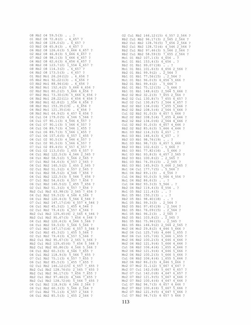
113
O8 Rb2 O4 59.5(3) . . ?
O1 Rb2 O8 72.8(2) . 6_657 ?
O5 Rb2 O8 129.0(2) . 6_657 ?
O3 Rb2 O8 65.8(3) . 6_657 ?
O6 Rb2 O8 126.6(3) 5_666 6_657 ?
O2 Rb2 O8 46.8(3) 5_666 6_657 ?
O7 Rb2 O8 98.1(3) 5_666 6_657 ?
O4 Rb2 O8 62.6(3) 6_656 6_657 ?
O8 Rb2 O8 123.7(2) 1_554 6_657 ?
O8 Rb2 O8 114.3(2) . 6_657 ?
O4 Rb2 O8 173.5(3) . 6_657 ?
O1 Rb2 Mo1 26.24(12) . 6_656 ?
O5 Rb2 Mo1 92.22(13) . 6_656 ?
O3 Rb2 Mo1 88.94(14) . 6_656 ?
O6 Rb2 Mo1 152.4(2) 5_666 6_656 ?
O2 Rb2 Mo1 80.2(2) 5_666 6_656 ?
O7 Rb2 Mo1 73.30(19) 5_666 6_656 ?
O4 Rb2 Mo1 28.22(11) 6_656 6_656 ?
O8 Rb2 Mo1 62.8(2) 1_554 6_656 ?
O8 Rb2 Mo1 153.35(19) . 6_656 ?
O4 Rb2 Mo1 121.35(14) . 6_656 ?
O8 Rb2 Mo1 64.9(2) 6_657 6_656 ?
O4 Cu1 O4 179.0(5) 4_546 5_566 ?
O4 Cu1 O7 90.1(3) 4_546 6_557 ?
O4 Cu1 O7 90.1(3) 5_566 6_557 ?
O4 Cu1 O6 89.7(3) 4_546 1_455 ?
O4 Cu1 O6 89.7(3) 5_566 1_455 ?
O7 Cu1 O6 157.6(5) 6_557 1_455 ?
O4 Cu1 O2 90.5(3) 4_546 6_557 ?
O4 Cu1 O2 90.5(3) 5_566 6_557 ?
O7 Cu1 O2 89.4(5) 6_557 6_557 ?
O6 Cu1 O2 113.0(5) 1_455 6_557 ?
O4 Cu1 Rb2 122.5(3) 4_546 2_565 ?
O4 Cu1 Rb2 58.5(2) 5_566 2_565 ?
O7 Cu1 Rb2 54.6(3) 6_557 2_565 ?
O6 Cu1 Rb2 140.5(2) 1_455 2_565 ?
O2 Cu1 Rb2 51.3(2) 6_557 2_565 ?
O4 Cu1 Rb2 58.5(2) 4_546 7_656 ?
O4 Cu1 Rb2 122.5(3) 5_566 7_656 ?
O7 Cu1 Rb2 54.6(3) 6_557 7_656 ?
O6 Cu1 Rb2 140.5(2) 1_455 7_656 ?
O2 Cu1 Rb2 51.3(2) 6_557 7_656 ?
Rb2 Cu1 Rb2 63.98(3) 2_565 7_656 ?
O4 Cu1 Rb2 59.5(3) 4_546 4_546 ?
O4 Cu1 Rb2 120.4(3) 5_566 4_546 ?
O7 Cu1 Rb2 147.17(14) 6_557 4_546 ?
O6 Cu1 Rb2 45.3(2) 1_455 4_546 ?
O2 Cu1 Rb2 79.4(3) 6_557 4_546 ?
Rb2 Cu1 Rb2 129.45(4) 2_565 4_546 ?
Rb2 Cu1 Rb2 95.67(3) 7_656 4_546 ?
O4 Cu1 Rb2 120.4(3) 4_546 5_566 ?
O4 Cu1 Rb2 59.5(3) 5_566 5_566 ?
O7 Cu1 Rb2 147.17(14) 6_557 5_566 ?
O6 Cu1 Rb2 45.3(2) 1_455 5_566 ?
O2 Cu1 Rb2 79.4(3) 6_557 5_566 ?
Rb2 Cu1 Rb2 95.67(3) 2_565 5_566 ?
Rb2 Cu1 Rb2 129.45(4) 7_656 5_566 ?
Rb2 Cu1 Rb2 60.86(3) 4_546 5_566 ?
O4 Cu1 Rb2 60.3(3) 4_546 7_655 ?
O4 Cu1 Rb2 118.9(3) 5_566 7_655 ?
O7 Cu1 Rb2 75.1(3) 6_557 7_655 ?
O6 Cu1 Rb2 85.5(3) 1_455 7_655 ?
O2 Cu1 Rb2 146.12(15) 6_557 7_655 ?
Rb2 Cu1 Rb2 128.76(5) 2_565 7_655 ?
Rb2 Cu1 Rb2 96.17(3) 7_656 7_655 ?
Rb2 Cu1 Rb2 97.46(3) 4_546 7_655 ?
Rb2 Cu1 Rb2 128.72(4) 5_566 7_655 ?
O4 Cu1 Rb2 118.9(3) 4_546 2_564 ?
O4 Cu1 Rb2 60.3(3) 5_566 2_564 ?
O7 Cu1 Rb2 75.1(3) 6_557 2_564 ?
O6 Cu1 Rb2 85.5(3) 1_455 2_564 ?
O2 Cu1 Rb2 146.12(15) 6_557 2_564 ?
Rb2 Cu1 Rb2 96.17(3) 2_565 2_564 ?
Rb2 Cu1 Rb2 128.76(5) 7_656 2_564 ?
Rb2 Cu1 Rb2 128.72(4) 4_546 2_564 ?
Rb2 Cu1 Rb2 97.46(3) 5_566 2_564 ?
Rb2 Cu1 Rb2 58.59(3) 7_655 2_564 ?
Mo1 O1 Rb2 107.1(3) 6_656 . ?
Mo1 O1 Rb1 153.4(3) 6_656 . ?
Rb2 O1 Rb1 99.07(18) . . ?
Mo1 O1 Rb1 101.6(3) 6_656 2_564 ?
Rb2 O1 Rb1 99.9(2) . 2_564 ?
Rb1 O1 Rb1 77.56(15) . 2_564 ?
Mo1 O1 Rb1 96.0(3) 6_656 5_666 ?
Rb2 O1 Rb1 99.4(2) . 5_666 ?
Rb1 O1 Rb1 75.12(15) . 5_666 ?
Rb1 O1 Rb1 148.6(2) 2_564 5_666 ?
Mo2 O2 Mo2 32.2(3) 7_655 2_564 ?
Mo2 O2 Cu1 130.8(7) 7_655 6_657 ?
Mo2 O2 Cu1 130.8(7) 2_564 6_657 ?
Mo2 O2 Rb2 134.0(6) 7_655 5_666 ?
Mo2 O2 Rb2 108.5(4) 2_564 5_666 ?
Cu1 O2 Rb2 91.0(3) 6_657 5_666 ?
Mo2 O2 Rb2 108.5(4) 7_655 4_646 ?
Mo2 O2 Rb2 134.0(6) 2_564 4_646 ?
Cu1 O2 Rb2 91.0(3) 6_657 4_646 ?
Rb2 O2 Rb2 85.6(3) 5_666 4_646 ?
Mo1 O3 Rb2 114.3(3) 6_657 . ?
Mo1 O3 Rb1 146.6(3) 6_657 . ?
Rb2 O3 Rb1 98.76(19) . . ?
Mo1 O3 Rb1 98.7(3) 6_657 5_666 ?
Rb2 O3 Rb1 102.6(2) . 5_666 ?
Rb1 O3 Rb1 77.82(16) . 5_666 ?
Mo1 O3 Rb1 93.8(3) 6_657 2_565 ?
Rb2 O3 Rb1 100.8(2) . 2_565 ?
Rb1 O3 Rb1 74.35(15) . 2_565 ?
Rb1 O3 Rb1 145.9(2) 5_666 2_565 ?
Mo1 O4 Cu1 177.7(5) . 5_566 ?
Mo1 O4 Rb2 89.1(3) . 6_556 ?
Cu1 O4 Rb2 93.0(3) 5_566 6_556 ?
Mo1 O4 Rb2 86.6(3) . . ?
Cu1 O4 Rb2 93.3(3) 5_566 . ?
Rb2 O4 Rb2 119.4(3) 6_556 . ?
Mo1 O5 Rb2 111.4(3) . . ?
Mo1 O5 Rb1 150.2(3) . . ?
Rb2 O5 Rb1 98.40(18) . . ?
Mo1 O5 Rb1 99.3(3) . 2_564 ?
Rb2 O5 Rb1 97.45(19) . 2_564 ?
Rb1 O5 Rb1 76.09(15) . 2_564 ?
Mo1 O5 Rb1 96.2(3) . 2_565 ?
Rb2 O5 Rb1 103.8(2) . 2_565 ?
Rb1 O5 Rb1 75.96(15) . 2_565 ?
Rb1 O5 Rb1 146.9(2) 2_564 2_565 ?
Mo2 O6 Mo2 29.8(2) 4_646 5_666 ?
Mo2 O6 Cu1 125.7(6) 4_646 1_655 ?
Mo2 O6 Cu1 125.7(6) 5_666 1_655 ?
Mo2 O6 Rb2 100.2(3) 4_646 4_646 ?
Mo2 O6 Rb2 121.9(4) 5_666 4_646 ?
Cu1 O6 Rb2 106.4(4) 1_655 4_646 ?
Mo2 O6 Rb2 121.9(4) 4_646 5_666 ?
Mo2 O6 Rb2 100.2(3) 5_666 5_666 ?
Cu1 O6 Rb2 106.4(4) 1_655 5_666 ?
Rb2 O6 Rb2 86.2(3) 4_646 5_666 ?
Mo2 O7 Mo2 31.1(2) 5_667 4_647 ?
Mo2 O7 Cu1 142.0(8) 5_667 6_657 ?
Mo2 O7 Cu1 142.0(8) 4_647 6_657 ?
Mo2 O7 Rb2 121.9(5) 5_667 4_646 ?
Mo2 O7 Rb2 100.4(4) 4_647 4_646 ?
Cu1 O7 Rb2 94.7(3) 6_657 4_646 ?
Mo2 O7 Rb2 100.4(4) 5_667 5_666 ?
Mo2 O7 Rb2 121.9(5) 4_647 5_666 ?
Cu1 O7 Rb2 94.7(3) 6_657 5_666 ?

114
Rb2 O7 Rb2 80.7(3) 4_646 5_666 ?
Mo2 O8 Rb1 176.3(8) . 2_565 ?
Mo2 O8 Rb2 92.7(5) . 1_556 ?
Rb1 O8 Rb2 90.7(3) 2_565 1_556 ?
Mo2 O8 Rb2 85.1(5) . . ?
Rb1 O8 Rb2 94.3(4) 2_565 . ?
Rb2 O8 Rb2 121.7(4) 1_556 . ?
Mo2 O8 Rb2 87.2(5) . 6_557 ?
Rb1 O8 Rb2 90.1(3) 2_565 6_557 ?
Rb2 O8 Rb2 115.3(4) 1_556 6_557 ?
Rb2 O8 Rb2 122.7(4) . 6_557 ?
_diffrn_measured_fraction_theta_max 0.996
_diffrn_reflns_theta_full 30.02
_diffrn_measured_fraction_theta_full 0.996
_refine_diff_density_max 2.333
_refine_diff_density_min -1.226
_refine_diff_density_rms 0.228

115
APPENDIX 6 – LETTERS OF PERMISSION

116
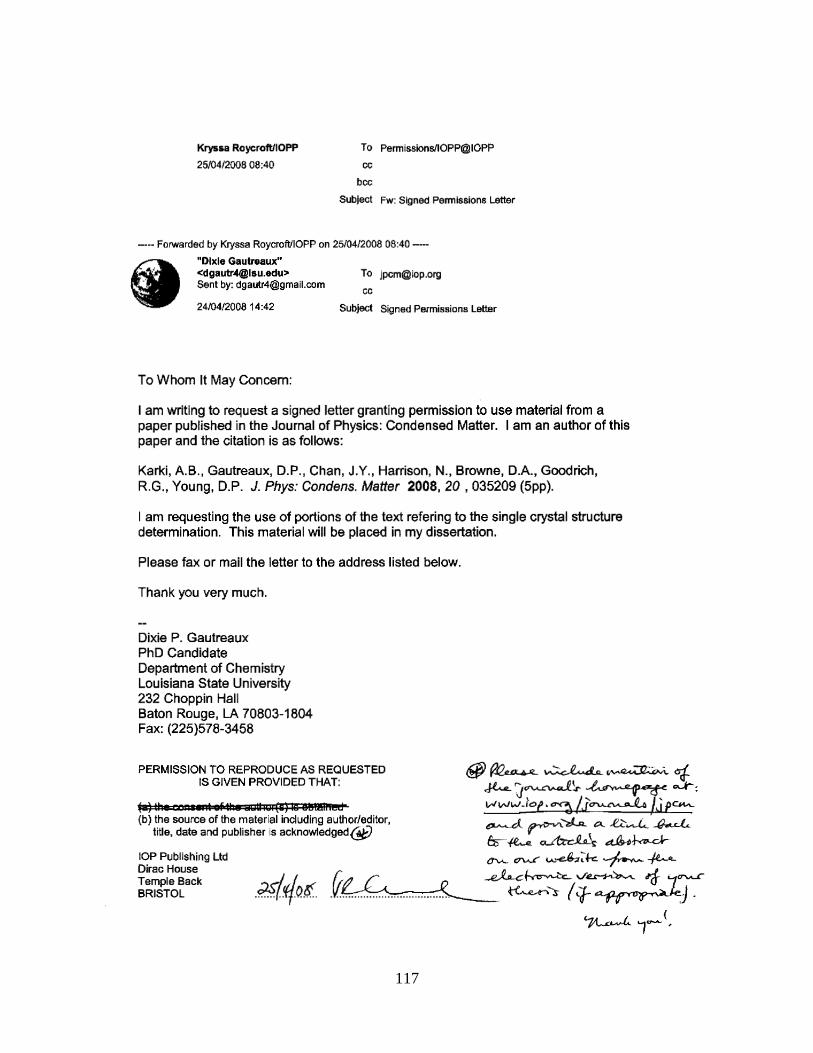
117

118

119

120
VITA
Dixie Plaisance Gautreaux was born in April 1982, in Lockport, Louisiana, to her parents
Joey and Kate Plaisance. She is the wife of Jarred Gautreaux of Lockport, Louisiana, and
mother of Elise Reneé. She has one younger sister, Josie Plaisance Eschete. In May 2000, Dixie
graduated sixth in her class from Central Lafourche High School in Mathews, Louisiana. Dixie
received numerous academic and music scholarships to universities throughout the state. She
attended Tulane University in New Orleans, Louisiana on a full Legislative scholarship from
August 2000-May 2001, where she majored in chemistry and was a member of the Tulane
Symphonic Winds and Green Wave Basketball Band. In August, 2001, she transferred to
Nicholls State University in Thibodaux, Louisiana, where she majored in chemistry and was the
president of the Nicholls Chemical Sciences Society. She was also a member of the NSU
Concert Band, Symphonic Winds, and the Pride of NSU Marching Band. She received a
Bachelor of Science in chemistry (cum laude) from Nicholls State University in December 2003.
Dixie began her graduate career at Louisiana State University in August, 2004, and
received a Louisiana Board of Regents Fellowship. She joined the Chan group in January 2005,
and began her doctoral research on ternary rare earth antimonides. She attended and presented
posters at national scientific meetings: the 24th
Rare Earth Research Conference in Keystone,
Colorado, the 232nd
ACS National Meeting & Exposition in San Francisco, California, and the
International Conference on Strongly Correlated Electron Systems in Houston, Texas. In 2006,
she was chosen to be a member of the US delegation at the 56th
Meeting of the Nobel Laureates
and Students in Lindau, Germany. In 2007, she was awarded a Strongly Correlated Electron
Systems Conference Young Investigator Award and a Proctor and Gamble Research Award. She
was awarded another Proctor and Gamble Research award in 2008. She was an officer on the

121
2005-2006 Chemistry Graduate Student Council. She was also very active in the department’s
service learning program where she visited nearby schools and performed chemistry
demonstrations for the students.
Dixie will graduate from Louisiana State University on August 8, 2008, with a Doctor of
Philosophy degree in chemistry. She has chosen a career in academics where she can teach and
inspire young minds for years to come.