Investigation into the Pressure-Driven Extensionof the EPANET Hydraulic Simulation Modelfor Water Distribution Systems

Alemtsehay G. Seyoum1& Tiku T. Tanyimboh1

Received: 10 December 2015 /Accepted: 5 September 2016 /Published online: 29 September 2016# The Author(s) 2016. This article is published with open access at Springerlink.com

Abstract Several hydraulic modelling approaches have been proposed previously to simulatepressure - deficient operating conditions in water distribution networks more realistically. EPANET-PDX is a pressure-driven extension of the EPANET 2 hydraulic simulation model that has anembedded logistic nodal head-flow function. The pressure-driven analysis algorithm in EPANET-PDX was investigated, to improve its performance under conditions of extremely low pressure. Byintegrating a line minimization procedure fully in the computational solution of the system ofequations, the algorithm’s consistency was improved by increasing its computational efficiencyunder conditions of extremely low pressure. The examples considered demonstrated that thepressure-driven analysis algorithm proposed is robust, computationally efficient, and the lineminimization procedure is applied frequently. Overall, the results suggest that the algorithm isreliable. The formulation proposed is significantly faster than the previousmodel under conditions ofextremely low pressure. The hydraulic and water quality modelling functionality of EPANET 2waspreserved. For the operating conditions with satisfactory pressure, where direct comparisons withEPANET 2 were possible, EPANET 2 was consistently faster.

Keywords Nodal head-flow function .Water distribution network . Lineminimization .

Evolutionary optimization . Global gradient algorithm . Pressure-driven analysis

Water Resour Manage (2016) 30:5351–5367DOI 10.1007/s11269-016-1492-6

Electronic supplementary material The online version of this article (doi:10.1007/s11269-016-1492-6)contains supplementary material, which is available to authorized users.

* Tiku T. Tanyimbohtiku.tanyimboh@strath.ac.uk

1 Department of Civil and Environmental Engineering, University of Strathclyde, James Weir Building,75 Montrose Street, Glasgow, G1 1XJ, UK

1 Introduction

Hydraulic simulation models of water distribution networks are invaluable for design andoperation purposes. They help predict the properties of the flow including water quality undernormal and abnormal operating conditions. Moreover, there is increasing emphasis on theapplication of hydraulic simulation models for solving optimisation problems by combiningthem with evolutionary algorithms (Kougias and Theodossiou 2013; Méndez et al. 2013; Diniand Tabesh 2014; Bragalli et al. 2016). The simulation models evaluate the equations forconservation of mass and energy and other properties such as nodal pressures (Seifollahi-Aghmiuni et al. 2013; Kang and Lansey 2014; Tao et al. 2014; Yang and Boccelli 2014;Laucelli and Giustolisi 2015; Kun et al. 2015). Evolutionary algorithms, by nature, oftengenerate numerous infeasible candidate solutions. While conventional demand-driven hydrau-lic simulation models (Rossman 2000; Spiliotis and Tsakiris 2011) are incapable of simulatingpressure-deficient conditions or infeasible solutions satisfactorily, pressure-driven models(Gorev and Kodzhespirova 2013; Tsakiris and Spiliotis 2014) do so realistically.

Evolutionary algorithms are essentially unconstrained optimisation procedures. On the otherhand, many real world optimisation problems have multiple constraints and, consequently, theneed for satisfactory approaches for incorporating constraints arises. Previous studies havedemonstrated the benefits of explicitly maintaining infeasible solutions among the candidatesolutions for single- and multi-objective constrained optimization problems (Singh et al. 2008;Ray et al. 2009). For example, some recent evolutionary optimization algorithms that retaininfeasible solutions until the last generation achieved good results in terms of the convergencerate and quality of solutions (Siew and Tanyimboh 2012b; Saleh and Tanyimboh 2013, 2014).

Considering the optimization of real-world networks with hundreds or thousands of pipes,where the computational time for evaluating millions of candidate solutions to carry outmultiple runs of an evolutionary algorithm could be prohibitive, a computationally efficientand robust pressure-driven simulation algorithm is vital. Very recently, Elhay et al. (2015)emphasized the urgent need for hydraulic models that are suitable for extreme operatingconditions and/or extreme events e.g. electrical power failure and terrorist attacks.

The pressure-driven simulation algorithm in this article builds on the pressure-dependentextension of the EPANET hydraulic simulator, i.e. EPANET-PDX (Siew and Tanyimboh2012a). EPANET-PDX has an integrated logistic nodal head-flow function (Tanyimboh andTempleman 2010) plus a line minimization procedure that facilitates convergence in thecomputational solution of the constitutive equations. This paper describes the EPANET-PDXalgorithm in detail and addresses weaknesses uncovered under conditions of extremely lowpressure (Seyoum 2015).

The modelling functionality of EPANET 2 (Rossman 2000) was preserved in full includingextended period simulation and water quality modelling (Seyoum and Tanyimboh 2014). Bycontrast, some investigations into pressure-driven analysis (e.g. Kovalenko et al. 2014; Elhayet al. 2015) did not consider extended period simulation. Furthermore, they excluded keyelements e.g. tanks, pumps and control devices. Control devices (e.g. pressure regulatingvalves) make the constitutive equations for water distribution systems difficult to solve due toconvergence problems (Rossman 2007; Deuerlein et al. 2009; Kovalenko et al. 2014; Elhayet al. 2015). While Tanyimboh and colleagues (Tanyimboh et al. 2003; Tanyimboh andTempleman 2010) included pumps and control devices, extended period simulation was notconsidered. An extensive review of pressure-driven simulation and its applications is availablein Abdy Sayyed et al. (2015). Other recent works on head-driven simulation include Elhay

5352 Seyoum A.G., Tanyimboh T.T.

et al. (2015) and Sivakumar and Prasad (2015). Reviews of nodal head-flow relationships areavailable in Ciaponi et al. (2015) and Vairagade et al. (2015).

2 Formulation of The Pressure-Driven Simulation Model

The EPANET 2 hydraulic simulator (Rossman 2000) uses the global gradient algorithm (Todini andPilati 1988) to solve the constitutive equations. Siew andTanyimboh (2012a) extended the algorithmby enabling it to simulate pressure-deficient conditions realistically. The pressure dependent modelknown as EPANET-PDX integrates the continuous nodal head-flow function that Tanyimboh andTempleman (2010) proposed in the constitutive equations. The nodal head-flow function is

Qni Hnið Þ ¼ Qnreqiexp αi þ βiHnið Þ

1þ exp αi þ βiHnið Þ ð1Þ

Its first derivative is

dQni Hnið ÞdHni

¼ Qnreqi βiexp αi þ βiHnið Þ

1þ exp αi þ βiHnið Þð Þ2 ð2Þ

where, for node i, Qni and Hni are the flow and head, respectively;Qnreqi is the demand; αi andβi are parameters that are determined by calibration with field data. A Monte Carlo simulationprocedure for calibrating αi and βi is available in Ciaponi et al. (2015).

Tanyimboh and Templeman (2010) provided a generic procedure for estimating αi and βi

that may be summarized briefly as follows.

Qni Hnmini

� � ¼ ε1Qnreqi ð3Þ

Qni Hnreqið Þ ¼ 1−ε2ð ÞQnreqi ð4Þwhere Hni

min and Hnireq are, respectively, the head below which flow at node i is unacceptably

low or effectively zero, and above which the demand is satisfied in full effectively. ε1 and ε2represent small tolerances that may be selected to suit the circumstances, for example, say ε1 =0.01 and ε2 = 0.001 (as in Tanyimboh and Templeman 2010). Kovalenko et al. (2014) adoptedε1 = ε2 = 0.001. Self-evidently the two values need not be identical, and any suitable combi-nation may be used. Eq. 3 implies that the available flow would be practically zero at Hni≈Hnmin

i : Similarly, Eq. 4 implies that the available flow would be practically satisfactory atHni≈Hnreqi : Illustrative examples are available in Ciaponi et al. (2015).

Eq. 1 represents a family of curves, and ε1 and ε2 lead to values of αi and βi that adjust theshape of the nodal head-flow function in Eq. 1. Approximate values of αi and βi may beobtained by substituting the values of Hni

min, Hnireq, ε1 and ε2 in Eqs. 3 and 4 the solution of

which provides the values of αi and βi. Following Tanyimboh and Templeman (2010), ε1 andε2 were taken as 0.01 and 0.001, respectively.

The system of equations applied in the global gradient algorithm is

A11 ⋮ A12

⋯ ⋯ ⋯A21 ⋮ 0

24

35

Qp⋯Hn

24

35 ¼

−A10H0

⋯−Qnreq

24

35 ð5Þ

Pressure Driven Extension of the EPANET Model 5353

A11 is a diagonal matrix whose elements are Kij Qpij� �n f −1

; Kij and nf are the resistance

coefficient and flow exponent in the head loss formula respectively; Qpij is the flow rate inpipe ij. A12 and A10 are the incidence matrices relating the pipes to the nodes with unknownand known heads, respectively. The elements of the incidence matrices are: −1 for pipe flowsaway from a node, +1 for pipe flows towards a node and 0 for pipes that are not connected tothe node under consideration. A21 = (A12)

T is the transpose of A12. Qp is the column vector ofthe unknown pipe flow rates. Hn and H0 are column vectors for the unknown and knownnodal heads, respectively. Qnreq is the column vector for the required nodal supplies.

To incorporate the nodal head-flow function, Eq. 5 is re-formulated as

A11 ⋮ A12

⋯ ⋯ ⋯A21 ⋮ A22

24

35

Qp⋯Hn

24

35 ¼

−A10H0

⋯0

24

35 ð6Þ

A22 is a diagonal matrix with elements Qni(Hni)/Hni; Qni(Hni) is the nodal head-flowfunction in Eq. 1. Thus, Eq. 6 may be rearranged as.

−A11 ⋮ A12

⋯ ⋯ ⋯A21 ⋮ A22

24

35

Qp⋯Hnk

k24

35þ

−A10H0

⋯0

24

35 ¼ −

f 1⋯f 2

24

35 ð7Þ

where the vectors f1 = f1(Qn, Hn) and f2 = f2(Qn, Hn) indicate the errors, for any givenapproximate solution (Qn, Hn)T; at the solution, both f1and f2 should be zero.

Considering Eq. 7, Eq. 6 may be solved by successive linearization using a first orderTaylor series expansion that gives

D11 ⋮ A12

⋯ ⋯ ⋯A21 ⋮ D22

24

35 Qpkþ1−Qpk

⋯Hnkþ1−Hnk

24

35 ¼ −

A11 ⋮ A12

⋯ ⋯ ⋯A21 ⋮ A22

24

35 Qpk

⋯Hnk

24

35þ

−A10H0

⋯0

24

35 ð8Þ

D11 is a diagonal matrix of the derivatives of the pipe head losses with respect to the pipe

flow rates, whose elements are nKij Qpij� �n f −1

; D22 is a diagonal matrix of the derivatives of

the nodal head-flow function with respect to the nodal heads, whose elements are described inEq. 2; k is the iteration number. Eq. (8) gives the following routine for computing the nodalheads and pipe flows iteratively.

Hnkþ1 ¼ A−1F ð9Þ

Qpkþ1 ¼ Qpk−D−111 A11Qpk þ A12Hnkþ1 þ A10H0

� � ð10Þ

In the above equations, i.e. Eq. 9 and 10,

A ¼ A21D−111A12−D22 ð11Þ

5354 Seyoum A.G., Tanyimboh T.T.

F ¼ −A21D11−1A11Qpk−A21D11

−1A10H0−D22Hnk þ A22Hnk þ A21Qpk ð12ÞThe procedure described above is for steady-state analysis. Extended period simulation may

be carried out as described in Rossman (2000) and Siew and Tanyimboh (2010).EPANET-PDX utilizes line minimization (Dennis and Schnabel 1996; Press et al. 2007) to

help ensure global convergence in the computational solution of Eqs. 7 and 8. However, in anattempt to exploit the excellent computational properties of EPANET 2, the line minimizationwas not optimized in Siew and Tanyimboh (2012a). While the applications to date suggest thatthe strategy works well in general (Seyoum and Tanyimboh 2014; Siew et al. 2014, 2016),relatively poor and inconsistent performance was discovered subsequently, under conditions ofextremely low pressure (Seyoum 2015). For the networks investigated, this correspondsroughly to a demand satisfaction of less than around 10 %.

The algorithm proposed herein allows unimpeded application of the line minimizationprocedure and, as a result, the computational efficiency is more consistent under all operatingconditions. Overall, the number of minor iterations (i.e. iterations of the line minimizationalgorithm) has increased substantially while the number of major iteration (i.e. iterations of theglobal gradient algorithm) has decreased.

3 Details of The Computational Solution Procedure

The equations for conservation of energy and mass in Eq. 7 are:

f 1 Hn;Qpð Þ ¼ A11Qpk þ A12Hnk þ A10H0 ð13Þ

f 2 Hn;Qpð Þ ¼ A21Qpk þ A22Hnk ð14ÞTogether, Eqs. 13 and 14 are a system of simultaneous non-linear equations, i.e. f = f(Hn,

Qp) = (f1, f2)T, the solution of which is required. The aim of the line minimization procedure is

to find an appropriate fraction λ of the Newton step δ = (δHn, δQp)T that decreases thefunction g in Eq. 15 sufficiently.

g ¼ 1

2f : f ð15Þ

where f.f = fTf is the 2-norm of the vector of the system of equations f; δHn and δQp are thevectors of the changes in the nodal heads and pipe flow rates, respectively. Given the scaler λ,the nodal heads Hn are updated iteratively as

Hnkþ1 ¼ Hnk þ λ:δHn; 0 < λ≤1 ð16Þwhere k is the iteration number and δHn is the Newton step for the nodal heads. The pipeflow rates Qpk + 1 are then updated by substituting the newly obtained nodal heads Hnk + 1

into Eq. (10).In each iteration of the global gradient algorithm, the full Newton step δ is attempted first. If

the Newton step does not reduce the value of the function sufficiently, then backtracking alongthe Newton direction (i.e. the direction described by the elements of δ), aimed at obtaining abetter approximate solution of f(Hn,Qp) = 0, is carried out. The acceptance criterion for thenew iterate is (Press et al. 2007)

Pressure Driven Extension of the EPANET Model 5355

g Hnkþ1;Qpkþ1� �

≤g Hnk ;Qpk� �þ ϕ:∇g:δ; 0 < ϕ < 1 ð17Þ

where ϕ = 10−4(Dennis and Schnabel 1996; Press et al. 2007). ∇g is the gradient of g(Hn,Qp)and δ = (δHn, δQp)T is the Newton step and direction. Thus, ∇g.δ is the directionalderivative or the rate of change of g(Hn,Qp) in the Newton direction δ. The initial rate ofdecrease of g(Hn,Qp) is given in Press et al. (2007) as

∇g:δ ¼ f :Jð Þ: −J−1:f� � ¼ − f : f ð18Þ

where J is the Jacobian matrix that comprises the first partial derivatives of f = f(Hn,Qp) withrespect to the nodal heads Hni,∀i, and pipe flow rates Qpij,∀ij.

Backtracking is carried out if g(Hnk + 1,Qpk + 1) fails to meet the acceptance criterion inEq. (17). In the backtracking procedure, application of the updating scheme in Eq. (16) (i.e.Hnk + 1 = Hnk + λ . δHn; 0 < λ ≤1) converts g(Hnk+1, Qpk+1) into a function of λ only, g(λ).Backtracking seeks the value of λ that minimizes g(λ) and is accomplished by line minimization.In the first iteration of the line minimization, g(λ) is modelled as a quadratic function. If anyadditional iterations are required then g(λ) is modelled as a cubic function. The iterations continueuntil either Eq. (17) is satisfied or λ reaches a specified minimum allowable value λmin. Dennisand Schnabel (1996) and Press et al. (2007) employed λmin = 0.1 while Siew and Tanyimboh(2012a) used λmin= 0.2 to avoid excessively small steps. λmin= 0.2 was adopted herein. Details ofthe quadratic and cubic approximations of g(λ) and its solution are available in Press et al. (2007).

The flow chart in Fig. 1 shows the integration of the line minimization in the global gradientalgorithm. The global gradient algorithm starts with initial estimates of the nodal heads and pipeflow rates. The nodal elevations are taken as the initial nodal heads while the initial pipe flowrates are derived from an assumed velocity of 1 ft./s (0.3048 m/s). In each iteration of the globalgradient algorithm, the Euclidean norm of the energy and mass balance equations is checked.

It was observed that, in some cases, when λ reached λmin = 0.2, the norm failed to reduce inconsecutive iterations. If this situation arises, the algorithm calculates a new Newton step i.e.δ = (δHn, δQp)T as a major iteration. Before doing so, however, the nodal heads are updatedfirst with λ = λmin = 0.2 in Eq. 16 as shown Fig. 1. This additional measure was introduced tohelp prevent premature convergence as it enables the major iterations to resume from adifferent point by updating Hn without updating Qp at the same time. In the investigationsherein, though rare, without this extra measure, there were instances of spurious convergence.False convergence may occur if a local minimum of Eq. 15, g ¼ 1

2 f : f , is found that is not a

root of Eq. 7, i.e. f = f(Hn,Qp) = 0 (Press et al. 2007).The iterations of the global gradient algorithm continue until the convergence criteria are

fulfilled. The EPANET-PDX convergence criteria of 0.001 ft. (3.048 × 10−4 m) for themaximum change in the nodal heads and 0.001 cubic feet per second (2.832 × 10−5 m3/s)for the maximum change in the pipe flow rates between successive iterations (Siew andTanyimboh 2012a) were retained herein. The EPANET-PDX software was developed byupgrading the source code of EPANET 2.

4 Results and Discussion

Three examples are provided to illustrate the properties of the proposed algorithm. The firsttwo are networks taken from literature, mainly to illustrate the performance in terms of the

5356 Seyoum A.G., Tanyimboh T.T.

number of iterations and CPU time required for convergence. The third example demonstratesthe effectiveness on a real-world network, based on extended period simulation under variousoperating conditions including extremely low pressure.

All the simulations were carried out on an Intel Xeon workstation (with two processors ofCPU 2.4 GHz and RAM of 16 GB). For simplicity hereafter, the new algorithm is calledEPANET-PDX (0.2) while the original EPANET-PDX is called EPANET-PDX (0.1). In all thesimulations, the assumed head below which nodal flow is zero was taken as the nodalelevation. In all the examples considered, the previous and new algorithms yielded essentially

No

Start

Initialise and

Yes

Update by minimizing

using quadratic

approximation

Yes

Yes

No

Update nodal heads using the full

Newton step by setting λ=1

Norm

reduced?

GGA

converged?

Stop

Is this the first minor

iteration?

Update by

minimizing

using cubic

approximation

Solve hydraulic equations using

global gradient algorithm GGA

(Compute and )

or ?

No

No

Update nodal heads:

Yes

Fig. 1 Integration of line minimization in the global gradient algorithm (GGA)

Pressure Driven Extension of the EPANET Model 5357

identical solutions (i.e. nodal flows, nodal heads and pipe flows) while the latter requiredfewer, or the same number of, iterations of the global gradient algorithm, as illustrated in theAppendix (i.e. online supplementary data).

4.1 Steady State Analysis of Small Networks

Two examples were considered for illustration purposes, i.e. the six-loop and Anytownnetworks in Fig. 2. The first example relates to the network in Fig. 2a (Todini 2003) thathas one source, 11 demand nodes, 17 pipes of length 500 m and Hazen-Williams roughnesscoefficient of 130. The elevations of the nodes are: 80 m for nodes 3 and 10; 85 m for nodes 4,5, 7 and 9; 90 m for nodes 2, 6, 8 and 11; and 100 m for node 12. The demands in m3/s are:0.01 for nodes 8 and 12; 0.04 for nodes 4, 9 and 11; and 0.05 for nodes 2, 5–7 and 10. The pipediameters in mm are: 100 for pipes 7, 10, 13, 14, 16 and 17; 150 for pipes 3, 6, 9, 12 and 15;200 for pipes 2, 5, 8 and 11; and 250 for pipes 1 and 4.

Steady-state simulations were performed as follows. (a) Simulations with assumed requiredresidual pressures of 30 m, 20 m and 10 m at all the demand nodes with the source head fixedat 150 m. (b) Simulations with source heads of 150 m, 125 m, 100 m and 75 m with anassumed required residual pressure of 30 m at all the demand nodes. Table 1 summarises thecomputational performances of EPANET-PDX (0.1) and (0.2). Generally EPANET-PDX (0.2)required fewer iterations while the CPU times of both models were comparable. The nodalheads and flows of both models were essentially identical.

The second example is based on the BAnytown^ network (Fig. 2b) used previously as abenchmark optimisation problem (Walski et al. 1987). Siew and Tanyimboh (2012a) modified thesystem and operational data to create a pressure-deficient condition. They set the diameter of pipes10, 13, 14, 15, 16 and 25 as 0.3048 m (12 in); the diameters of the six pipes mentioned were to bedetermined in the optimization problem (Walski et al. 1987). Also, the demands at nodes 2, 4, 5, 9,10, 12 and 15 were taken as 3.155 l/s. Additional data for the pipes and nodes are available inWalski et al. (1987). Awater treatment plant supplies the network, with three identical pumps thatoperate in parallel. The water level in the treatment plant is fixed at 3.05 m (10 ft). The requiredpressure for all the demand nodes is 28.12 m (40 psi). The network has two storage tanks (Tanks41 and 42). Herein, the pipes that connect the tanks to the network were closed.

Using the base demands, and taking the demand factors (i.e. the nodal demand multipliers)as 1.0, a steady-state simulation of the modified network with the tanks closed showed therewas insufficient pressure, as only 87 % of the total demand was satisfied. Comparisons of thenodal heads and outflows for all the nodes showed that both EPANET-PDX (0.1) and (0.2)yielded essentially identical results. The number of iterations required by EPANET-PDX (0.1)and (0.2) to converge was 13 and 10, respectively. Both models required on average 0.04 s tocomplete the simulation.

4.2 Extended Period Simulation of Real World Network

An investigation was conducted based on a network that is a hydraulic demand zone (referredto hereafter as a water supply zone) in the UK. Figure 2c shows the network that comprises251 pipes of various lengths, 228 demand nodes (including the fire hydrants), 3 demandcategories and 29 fire hydrants; the pipe diameters range from 32 mm to 400 mm. The networkobtains water entirely from the neighbouring water supply zones through five variable-headsupply nodes (i.e. nodes R1-R5 in Fig. 2c). Details of the temporal variations in the demands

5358 Seyoum A.G., Tanyimboh T.T.

(b)

(a)

The Anytown network in Example 2

(c)

Example 1

Example 3

Fig. 2 Topologies of the networks investigated

Pressure Driven Extension of the EPANET Model 5359

and supply-node heads are available in Seyoum and Tanyimboh (2014). The range of variationin the heads at the supply nodes is insignificant. Therefore, here, to simplify the interpretationof the results, the supply nodes were modelled as constant-head nodes with water levels of155 m each.

The water utility provided the network and dynamic operational data from a geographicalinformation system database, and a calibrated EPANET model. The demand categoriescomprise domestic and 10-h commercial demands, and unaccounted for water (Kanakoudisand Gonelas 2016). There are 29 different fire demands of one hour each at the respective firehydrants. The head loss in the pipes due to friction is derived from the Darcy-Weisbachformula (Rossman 2000). The required residual head at all the demand nodes is 20 m.

All the analyses reported on this network consist of extended period simulations of 31 h,with a hydraulic time step of one hour. For each of the three simulation models considered, i.e.EPANET 2, EPANET-PDX (0.1) and (0.2), 66 extended period simulations were carried out intotal, for the normal and pressure-deficient conditions. The simulations included pipe closures(10 cases) and varying head levels at the supply nodes (56 cases).

4.2.1 Source Head Variations

The investigation covered all levels of demand satisfaction from zero to 100 %. Supply nodeheads from 75 m to 130 m in steps of 1 m were considered. Each model executed the 56simulations without convergence failures. EPANET-PDX (0.1) and (0.2) gave identical resultsof flow and pressure. The computational performance was assessed considering three scenar-ios, i.e. normal, low and extremely low pressure.

Normal pressure was taken as 99.9 % demand satisfaction and above, for the network as awhole. This corresponds to heads at the supply nodes from approximately 116 m to 130 m. Inthe extended period simulation, the number of major iterations required on average per steady-state simulation was 7.00, 5.00 and 5.16 for EPANET-PDX (0.1), EPANET-PDX (0.2) andEPANET 2, respectively. Figure 3a compares the CPU times. On average, EPANET-PDX (0.1)and (0.2) required about 0.27 s and 0.29 s, respectively, per extended period simulation,compared to 0.15 s for EPANET 2.

Table 1 Major iterations and CPU times for the network in Example 1

Variations in required nodalresidual heads

Variations in reservoir heads

Required residual heads (m) Reservoir heads (m)

30 a(88 %) 20 (89 %) 10 (91 %) 150 (88 %) 125 (71 %) 100 (29 %) 75 (0.04 %)

Number of major iterations

EPANET-PDX (0.1) 9 11 29 9 9 10 8

EPANET-PDX (0.2) 9 10 16 9 9 7 7

CPU times (seconds)

EPANET-PDX (0.1) 0.03 0.03 0.04 0.03 0.04 0.03 0.03

EPANET-PDX (0.2) 0.05 0.04 0.04 0.05 0.03 0.03 0.03

a The values in parentheses are the percentages of the total network demand satisfied

5360 Seyoum A.G., Tanyimboh T.T.

EPANET 2, in general, seemed more efficient and consistent. It is worth emphasizing,however, that EPANET 2 and EPANET-PDX apply convergence criteria that are different(Siew and Tanyimboh 2012a). The default criterion used in EPANET 2 is that the ratio of thesum of the absolute values of the changes in the pipe flow rates to the total flow in all the pipesshould be less than 0.001. Therefore, it is worth emphasizing also that the EPANET 2 resultsserve as a reference rather than a direct comparison. The CPU times refer to extended periodsimulations of 31 h with a hydraulic time step of one hour. Burger et al. (2015) compareddifferent demand-driven analysis solvers to EPANET 2 and concluded that EPANET 2 was thefastest for practical applications.

(a) Normal pressure conditions

(b) Pressure-deficient conditions

(c) Extremely low pressure conditions

0.7

0.8

0.9

1

0.0

0.2

0.4

0.6

0.8

116 120 124 128

DS

R

CP

U tim

e (

seconds)

Head at supply nodes (R1-R5) (m)

Normal pressure conditions

EPANET-PDX (0.1) EPANET-PDX (0.2) EPANET-2 Network DSR

0

0.2

0.4

0.6

0.8

1

0.0

0.2

0.4

0.6

0.8

88 92 96 100 104 108 112

DS

R

CP

U tim

e (

seconds)

Head at supply nodes (R1-R5) (m)

Pressure-deficent conditions

EPANET-PDX (0.1) EPANET-PDX (0.2) Network DSR

0

0.2

0.4

0.6

0.8

1

0.0

0.2

0.4

0.6

0.8

75 78 81 84 87

DS

R

CP

U t

ime (

seconds)

Head at supply nodes (R1-R5) (m)

Extremely low pressure conditions

EPANET-PDX (0.1) EPANET-PDX (0.2) Network DSR

Fig. 3 CPU times as a function ofpressure in the network inExample 3. DSR is the demandsatisfaction ratio, i.e. the ratio ofthe available flow to the requiredflow

Pressure Driven Extension of the EPANET Model 5361

The pressure-deficient condition was assumed to include demand satisfaction of 9.23 % to99.9 %, i.e. from just below satisfactory pressure to just above extremely low-pressure. Thecorresponding heads at the supply nodes were 88 m to 115 m approximately. EPANET 2results are not included in this scenario and the next, as it is not suitable for operatingconditions with insufficient pressure. The major iterations and CPU times were similar tothe normal operating condition. On average, the number of iterations per steady state simula-tion was 7.00 and 5.04 for EPANET-PDX (0.1) and EPANET-PDX (0.2), respectively. TheCPU times were comparable, i.e. 0.27 s and 0.29 s for EPANET-PDX (0.1) and EPANET-PDX(0.2) respectively, per extended-period simulation (Fig. 3b).

The performance under conditions of extremely low pressure is important from the perspec-tive of evolutionary optimisation algorithms that may generate extremely infeasible solutions.Recent results have demonstrated the advantages of retaining nondominated infeasible solu-tions until the end of the optimization (Siew and Tanyimboh 2012b; Eskandar et al. 2012; Salehand Tanyimboh 2013, 2014, 2016; Siew et al. 2014, 2016; Tanyimboh and Seyoum 2016) asinfeasible solutions usually contain useful genetic materials (Herrera et al. 1998).

Supply node heads from 75 m to 87 m, approximately, with network demand satisfactionbelow 9.23 %, were deemed extremely low (Fig. 3c). EPANET-PDX (0.2) achieved significantimprovements in both the number of iterations and CPU time. The average number ofiterations was 6.85 and 4.08 for EPANET-PDX (0.1) and EPANET-PDX (0.2), respectively.The average CPU time was 0.38 s and 0.28 s for EPANET-PDX (0.1) and EPANET-PDX(0.2), respectively. For supply node heads from 75 m to 81 m, EPANET-PDX (0.2) was up toaround 50 % faster.

4.2.2 Pipe Closures

In this scenario, the pipes from three supply nodes out of five (R1-R5) were closed. In total, 10cases were considered and it was observed that the nodal demands were fully satisfied in eachcase. Table 2 provides a summary of the results. On average, there were 6.77, 5.22 and 4.90iterations per steady state simulation for EPANET-PDX (0.1), EPANET-PDX (0.2) and

Table 2 Major iterations and CPU times for the pipe closures in Example 3

Closed SupplyNodes

Mean number of major iterations persteady-state simulation

CPU times for extended period simulations(seconds)

EPANET-PDX(0.1)

EPANET-PDX(0.2)

EPANET 2 EPANET-PDX(0.1)

EPANET-PDX(0.2)

EPANET 2

R1,2,3 6.969 5.250 4.875 0.197 0.202 0.137

R1,2,4 6.719 5.156 5.000 0.200 0.209 0.137

R1,2,5 6.781 5.250 4.875 0.193 0.207 0.140

R1,3,4 6.750 5.250 4.875 0.210 0.238 0.140

R1,3,5 6.563 5.188 4.844 0.197 0.202 0.147

R1,4,5 6.719 5.313 4.875 0.190 0.204 0.147

R2,3,4 6.781 5.125 4.844 0.200 0.205 0.147

R2,3,5 6.969 5.250 4.938 0.197 0.197 0.137

R2,4,5 6.656 5.125 4.969 0.200 0.202 0.140

R3,4,5 6.750 5.250 4.875 0.200 0.209 0.153

5362 Seyoum A.G., Tanyimboh T.T.

EPANET 2, respectively. The corresponding average CPU times were 0.20, 0.21 and 0.14 s,respectively, per extended period simulation.

4.2.3 Effectiveness of the Line Minimization

Figure 4a shows the number of minor iterations as a function of the pressure. Ingeneral, under conditions of extremely low pressure, EPANET-PDX (0.1) applied oneminor iteration per steady state simulation while EPANET-PDX (0.2) applied anaverage of 10.30. Figure 4b shows the number of minor iterations for the supply-node closures. On average, EPANET-PDX (0.2) performed 10.43 minor iterations persteady state simulation whereas EPANET-PDX (0.1) performed only 0.16. Overall, itseems that the line minimization in EPANET-PDX (0.1) served mainly as a safety netto avoid divergence of the major iterations.

Figure 5 shows the norm of the constitutive equations at successive iterations, for threetypical extended period simulations. Each simulation comprises 31 steady state simulations. Itis worth mentioning that the norm in Fig. 5 is based on cubic feet per second and feet, for flowcontinuity and head loss, respectively. In SI units (m3 s−1 and m), the values would be muchsmaller.

It was observed that for the network demand satisfaction of 0.01 % (Fig. 5c), the normincreased at the second iteration before decreasing consistently in subsequent iterations.Dennis and Schnabel (1996, pp. 129) discuss the circumstances in which the line minimizationmay loop indefinitely. This may arise if the Newton direction is not a descent direction. It may

(a) Mean number of minor iterations per steady state simulation as a function of pressure

(b) Mean number of minor iterations per steady state simulation for pipe closures

0

0.2

0.4

0.6

0.8

1

0

3

6

9

12

75 95 115 135

DS

R

Num

ber o

f line s

earch

evalu

ations

Head at supply nodes (R1-R5) (m)

EPANET-PDX (0.1) EPANET-PDX (0.2) Network DSR

0

3

6

9

12

Nu

mb

er o

f lin

e

se

arch

eva

lua

tio

ns

Closed supply nodes

EPANET-PDX (0.1) EPANET-PDX (0.2)

Fig. 4 Comparison of the minor iterations based on the network in Example 3

Pressure Driven Extension of the EPANET Model 5363

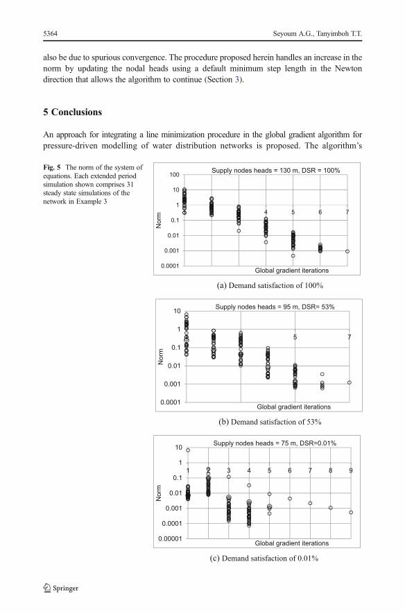
also be due to spurious convergence. The procedure proposed herein handles an increase in thenorm by updating the nodal heads using a default minimum step length in the Newtondirection that allows the algorithm to continue (Section 3).

5 Conclusions

An approach for integrating a line minimization procedure in the global gradient algorithm forpressure-driven modelling of water distribution networks is proposed. The algorithm’s

(a) Demand satisfaction of 100%

(b) Demand satisfaction of 53%

(c) Demand satisfaction of 0.01%

0.0001

0.001

0.01

0.1

1

10

100

1 2 3 4 5 6 7

Norm

Global gradient iterations

Supply nodes heads = 130 m, DSR = 100%

0.0001

0.001

0.01

0.1

1

10

1 3 5 7

Norm

Global gradient iterations

Supply nodes heads = 95 m, DSR= 53%

0.00001

0.0001

0.001

0.01

0.1

1

10

1 2 3 4 5 6 7 8 9

Norm

Global gradient iterations

Supply nodes heads = 75 m, DSR=0.01%

Fig. 5 The norm of the system ofequations. Each extended periodsimulation shown comprises 31steady state simulations of thenetwork in Example 3

5364 Seyoum A.G., Tanyimboh T.T.

performance was satisfactory when simulating two networks in the literature and a real-worldnetwork. For simulations based on the real-world network, the algorithm achieved significantimprovements in both the number ofmajor iterations (40%) andCPU time (26%), in conditions ofextremely low pressure, compared to Siew and Tanyimboh (2012a). In particular, for supply nodeheads from 75m to 81m, the CPU timewas reduced by up to 50% approximately. It may be notedalso, that the hydraulic andwater qualitymodelling functionality of EPANET2 has been preserved.

The algorithm proposed allows unimpeded application of the line minimization procedureand, as a result, the computational properties are more consistent under all operating conditions.Overall, the number of minor iterations (i.e. iterations of the line minimization algorithm) hasincreased substantially while the number of major iteration (i.e. iterations of the global gradientalgorithm) has decreased. Where direct comparisons with EPANET 2 were possible, i.e. foroperating conditions with satisfactory pressure, EPANET 2 was consistently faster.

Acknowledgment This project was funded in part by the UKEngineering and Physical Sciences Research Council(EPSRC Grant Reference EP/G055564/1), the British Government (Overseas Research Students Awards Scheme)and the University of Strathclyde. This financial support is acknowledged with thanks. The authors also thank Dr.Lewis Rossman of the United States Environmental Protection Agency, for assisting with the source code of theEPANET 2 computer program, and Veolia Water UK (now Affinity Water) for the support they provided.

Compliance with Ethical Standards

Conflict of Interest There is no conflict of interest.

Open Access This article is distributed under the terms of the Creative Commons Attribution 4.0 InternationalLicense (http://creativecommons.org/licenses/by/4.0/), which permits unrestricted use, distribution, and repro-duction in any medium, provided you give appropriate credit to the original author(s) and the source, provide alink to the Creative Commons license, and indicate if changes were made.

References

Abdy Sayyed MAH, Gupta R, Tanyimboh TT (2015) Noniterative application of EPANET for pressuredependent modelling of water distribution systems. Water Resour Manag 29(9):3227–3242

Bragalli C, Fortini M, Todini E (2016) Enhancing knowledge in water distribution networks via data assimilation.Water Resour Manag 30(11):3689–3706

Burger G, Sitzenfrei R, Kleidorfer M, Rauch W (2015) Quest for a new solver for EPANET 2. Journal of WaterResource Planning and Management. doi:10.1061/(ASCE)WR.1943-5452.0000596

Ciaponi C, Franchioli L, Murari E, Papiri S (2015) Procedure for defining a pressure-outflow relationshipregarding indoor demands in pressure-driven analysis of water distribution networks. Water Resour Manag29(3):817–832

Dennis JE, Schnabel RB (1996) Numerical methods for unconstrained optimization and nonlinear equations.SIAM, Philadelphia

Deuerlein J, Simpson A, Dempe S (2009) Modeling the behavior of flow regulating devices in water distributionsystems using constrained nonlinear programming. J Hydraul Eng 135(11):970–982

Dini M, Tabesh M (2014) A new method for simultaneous calibration of demand pattern and Hazen-Williamscoefficients in water distribution systems. Water Resour Manag 28:2021–2034

Elhay S, Piller O, Deuerlein J, Simpson A (2015) A robust, rapidly convergent method that solves the waterdistribution equations for pressure-dependent models. Journal of Water Resource Planning and Management.doi:10.1061/(ASCE)WR.1943-5452.0000578

Eskandar H, Sadollah A, Bahreininejad A, et al. (2012) Water cycle algorithm – a novel metaheuristicoptimization method for solving constrained engineering optimization problems. Comput Struct:110–111

Gorev NB, Kodzhespirova IF (2013) Noniterative implementation of pressure-dependent demands using thehydraulic analysis engine of EPANET 2. Water Resour Manag 27(10):3623–3630

Pressure Driven Extension of the EPANET Model 5365

Herrera F, Lozano M, Verdegay JL (1998) Tackling real-coded genetic algorithms: operators and tools forbehavioural analysis. Artif Intell Rev 12:265–319

Kanakoudis V, Gonelas K (2016) Analysis and calculation of the short and long run economic leakage level in awater distribution system. Water utility Journal 12:57–66

Kang D, Lansey K (2014) Novel approach to detecting pipe bursts in water distribution networks. J Water ResourPlan Manag 140(1):121–127

Kougias IP, Theodossiou NP (2013) Multi-objective pump scheduling optimization using harmony searchalgorithm and polyphonic HSA. Water Resour Manag 27(5):1249–1261

Kovalenko Y, Gorev NB, Kodzhespirova IF, Prokhorov E, Trapaga G (2014) Convergence of a hydraulic solverwith pressure-dependent demands. Water Resour Manag 28(4):1013–1031

Kun D, Tian-Yu L, Jun-Hui W, Jin-Song G (2015) Inversion model of water distribution systems fornodal demand calibration. J. Water Resour. Plann. Manage. doi:10.1061/(ASCE)WR.1943-5452.0000506

Laucelli D, Giustolisi O (2015) Vulnerability assessment of water distribution networks under seismic actions. JWater Resour Plann Manage. doi:10.1061/(ASCE)WR.1943-5452.0000478,04014082

Méndez M, Araya JA, Sanchez LD (2013) Automated parameter optimization of a water distribution system. JHydroinf 15(1):71–85

Press WH, Teukolsky SA, VetterlingWT, Flannery BP (2007) Numerical recipes: The art of scientific computing.Press, Cambridge University

Ray T, Singh HK, Isaacs A, Smith W (2009) Infeasibility driven evolutionary algorithm for constrainedoptimization, in Constraint Handling in Evolutionary Optimization Studies in Computational Intelligence:Vol.198. Springer, Berlin, pp. 145–165

Rossman LA (2000) EPANET 2 Users manual. Water supply and water resources division. National RiskManagement Research Laboratory, US EPA, Cincinnati

Rossman LA (2007) Discussion of BSolution for water distribution systems under pressure-deficient conditions^by Ang and Jowitt. Journal of Water Resource Planning and Management 133(6):566–567

Saleh SH, Tanyimboh TT (2013) Coupled topology and pipe size optimization of water distribution systems.Water Resour Manag 27(14):4795–4814

Saleh SH, Tanyimboh TT (2014) Optimal design of water distribution systems based on entropy and topology.Water Resour Manag 28(11):3555–3575

Saleh SHA, Tanyimboh TT (2016) Multi-directional maximum-entropy approach to the evolutionary designoptimization of water distribution systems. Water Resour Manag 30(6):1885–1901

Seifollahi-Aghmiuni S, Bozorg Haddad O, Mariño MA (2013) Water distribution network risk analysis undersimultaneous consumption and roughness uncertainties. Water Resour Manag 27(7):2595–2610

Seyoum AG (2015) Head dependent modelling and optimization of water distribution systems. PhD thesis,University of Strathclyde, Glasgow

Seyoum AG, Tanyimboh TT (2014) Pressure dependent network water quality modelling. Proceedings of ICE:Water Management 167(6):342–355

Siew C, Tanyimboh TT (2010) Pressure-dependent EPANET extension: Extended period simulation. 12thInternational Conference on Water Distribution Systems Analysis, Tucson, Arizona. doi:10.1061/41203(425)10

Siew C, Tanyimboh TT (2012a) Pressure-dependent EPANET extension. Water Resour Manag 26(6):1477–1498

Siew C, Tanyimboh TT (2012b) Penalty-free feasibility boundary convergent multi-objective evolu-tionary algorithm for the optimization of water distribution systems. Water Resour Manag 26(15):4485–4507

Siew C, Tanyimboh TT, Seyoum AG (2014) Assessment of penalty-free multi-objective evolutionary optimiza-tion approach for the design and rehabilitation of water distribution systems. Water Resour Manag 28(2):373–389

Siew C, Tanyimboh TT, Seyoum AG (2016) Penalty-free multi-objective evolutionary approach to optimizationof Anytown water distribution network. Water Resour Manag 30(11):3671–3688

Singh HK, Isaacs A, Ray T, Smith W (2008) Infeasibility driven evolutionary algorithm (IDEA) for engineeringdesign optimization. 21st Australiasian Joint Conference on. Artificial Intelligence AI-08:104–115

Sivakumar P, Prasad RK (2015) Extended period simulation of pressure-deficient networks using pressurereducing valves. Water Resour Manag 29(5):1713–1730

Spiliotis M, Tsakiris G (2011) Water distribution system analysis: Newton-Raphson method revisited. J HydraulEng ASCE 137(8):852–855

Tanyimboh TT, Seyoum AG (2016) Multiobjective evolutionary optimization of water distribution systems:Exploiting diversity with infeasible solutions. J Environ Manag 183:133–141. doi:10.1016/j.jenvman.2016.08.048

5366 Seyoum A.G., Tanyimboh T.T.

Tanyimboh TT, Templeman AB (2010) Seamless pressure deficient water distribution system model.Proceedings of ICE: Water Management 163(8):389–396

Tanyimboh TT, Tahar B, Templeman AB (2003) Pressure-driven modelling of water distribution systems. Waterscience and technology. Water Supply 3(1–2):255–261

Tao T, Huang H, Li F, Xin K (2014) Burst detection using an artificial immune network in water-distributionsystems. J. Water Resour. Plann. Manage. doi:10.1061/(ASCE)WR.1943-5452.0000405,04014027

Todini, E. (2003) A more realistic approach to the extended period simulation of water distribution networks.Advances in Water Supply Management, Maksimovic, C., Butler, D. and Memon, F.A. (eds.), Balkema,The Netherlands, pp.173–184.

Todini E, Pilati S (1988) In: Coulbeck B, Chun-Hou O (eds) A gradient algorithm for the analysis of pipenetworks. Computer applications in water supply: systems analysis and SIMULATION: Vol. 1. ResearchStudies Press, Taunton, pp. 1–20

Tsakiris G, Spiliotis M (2014) A Newton-Raphson analysis of urban water systems based on nodal head-drivenoutflow. European Journal of Environmental and Civil Engineering 18(8):882–896

Vairagade SA, Abdy Sayyed MAH, Gupta R (2015) Node head flow relationships in skeletonized waterdistribution networks for predicting performance under deficient conditions. World Environmental andWater Resources Congress, Austin, Texas

Walski TM, Brill ED, Gessler J, Goulter IC, Jeppson RM, Lansey K, Lee HL, Liebman JC, Mays L, Morgan DR,Ormsbee L (1987) Battle of the network models: epilogue. Journal of Water Resource Planning andManagement 113(2):191–203

Yang X, Boccelli D (2014) Bayesian approach for real-time probabilistic contamination source identification. J.Water Resour. Plann. Manage. doi:10.1061/(ASCE)WR.1943-5452.0000381,04014019

Pressure Driven Extension of the EPANET Model 5367