Investigation into the Assumptions for Lumped Capacitance Modelling of Turbocharger Heat Transfer

Richard Burke, Colin Copeland and Tomasz Duda

Abstract Heat transfer in turbochargers is often ignored for one-dimensional engine modelling, however this omission limits the usefulness of these models in the development for part load and transient operating conditions. Advanced heat transfer models have been proposed to account for these thermal effects based on the assumption that the compressor housing can be represented as a single lumped mass with heat and work transfer occurring separately. In this paper, both one- and three-dimensional modelling have been undertaken to assess the validity of these assumptions. One dimensional modelling showed that at low load conditions the magnitude of heat flow-ing to the compressor is the dominant effect causing errors in temperature predic-tions. In contrast at higher powers it is the distribution of heat transfer pre and post compression that have larger effects. Three-dimensional modelling subsequently showed that at low load the compressor housing remains warmer than the gases throughout the device. In contrast at high powers the compressed gas temperature can exceed the temperature of the housing on the front face of the compressor creat-ing significantly more complex heat flows that may not be captured by the simple model structures.

1. Introduction

Turbochargers are a vital component for enabling engine downsizing by recycling the energy in the exhaust gases to force a higher air flow through the engine and there-fore increase the engine power. The matching of a turbocharger to an engine is heavily reliant on zero- and one- dimensional modelling approaches with the first used for an initial sizing of the turbomachinery and the latter used for the refinement under full load, part load, altitude and transient operating conditions. Within the one-dimensional tools, turbochargers are modelled using characteristic performance maps that describe the behavior based on measurements taken on steady flow gas stands. The measurement process is based on the assumption of no heat transfer which is only valid for high turbocharger speeds where the mechanical power is much greater that heat flows. At lower shaft speeds, which are representative of common driving scenarios, the heat transfer becomes a significant part of the tem-perature rise in the compressor which limits the accuracy of modelling for operation in this region. A number of simplified heat transfer models have been proposed to pre-dict the heat transfer effects in this low speed region. This paper examines the as-sumptions for heat transfer between the compressor housing and intake gases using a 3D conjugate heat transfer simulation and quantifies the sensitivity of these as-sumptions in overall compressor performance prediction.

2. Heat transfer modelling for turbochargers Turbochargers are typically modelled in 1D engine simulations using performance maps based on data measured from steady state gas stands. These maps describe the flow and efficiency characteristics as described in equations 1 and 2 (for the compressor) whilst the speed of the device is determined using a power balance be-tween turbine and compressor according to equation 3.

�̇�𝑐 = 𝑓(𝑃𝑅𝑐, 𝑁𝑇)̇ (1)

𝜂𝑐 = 𝑓(𝑃𝑅𝑐, �̇�𝑐)̇ (2)

𝑑𝑁

𝑑𝑡=

60

2𝜋𝐼𝑇

(𝜏𝑡 − 𝜏𝑐)̇

(3)

The values for speed, mass flow and pressure ratio are measured directly; however isentropic efficiency is derived from gas temperature measurements at the inlet and outlet of the device according to equation 4. This is based on the assumption that the temperature rise across the compressor is a result only of work transfer, and hence any heat transfer that affects this temperature rise will compromise the accuracy of the efficiency.

𝜂𝑠,𝑐 =

𝑇1 ((𝑃2

𝑃1)

𝛾−1𝛾

− 1)

𝑇2 − 𝑇1

(4)

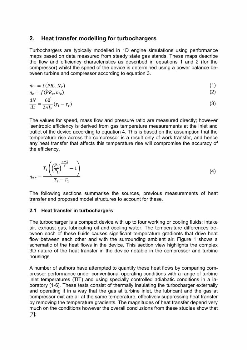
The following sections summarise the sources, previous measurements of heat transfer and proposed model structures to account for these. 2.1 Heat transfer in turbochargers The turbocharger is a compact device with up to four working or cooling fluids: intake air, exhaust gas, lubricating oil and cooling water. The temperature differences be-tween each of these fluids causes significant temperature gradients that drive heat flow between each other and with the surrounding ambient air. Figure 1 shows a schematic of the heat flows in the device. This section view highlights the complex 3D nature of the heat transfer in the device notable in the compressor and turbine housings A number of authors have attempted to quantify these heat flows by comparing com-pressor performance under conventional operating conditions with a range of turbine inlet temperatures (TIT) and using specially controlled adiabatic conditions in a la-boratory [1-6]. These tests consist of thermally insulating the turbocharger externally and operating it in a way that the gas at turbine inlet, the lubricant and the gas at compressor exit are all at the same temperature, effectively suppressing heat transfer by removing the temperature gradients. The magnitudes of heat transfer depend very much on the conditions however the overall conclusions from these studies show that [7]:

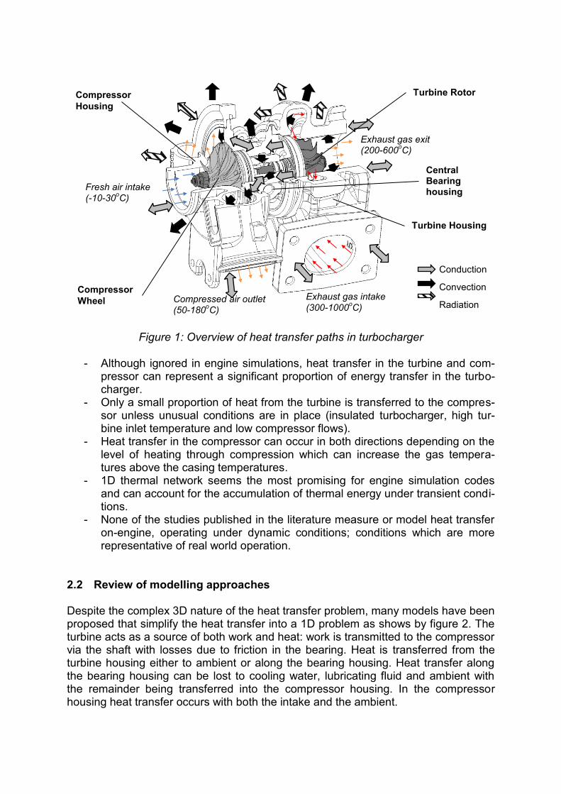
Figure 1: Overview of heat transfer paths in turbocharger

- Although ignored in engine simulations, heat transfer in the turbine and com-

pressor can represent a significant proportion of energy transfer in the turbo-charger.

- Only a small proportion of heat from the turbine is transferred to the compres-sor unless unusual conditions are in place (insulated turbocharger, high tur-bine inlet temperature and low compressor flows).

- Heat transfer in the compressor can occur in both directions depending on the level of heating through compression which can increase the gas tempera-tures above the casing temperatures.

- 1D thermal network seems the most promising for engine simulation codes and can account for the accumulation of thermal energy under transient condi-tions.

- None of the studies published in the literature measure or model heat transfer on-engine, operating under dynamic conditions; conditions which are more representative of real world operation.

2.2 Review of modelling approaches Despite the complex 3D nature of the heat transfer problem, many models have been proposed that simplify the heat transfer into a 1D problem as shows by figure 2. The turbine acts as a source of both work and heat: work is transmitted to the compressor via the shaft with losses due to friction in the bearing. Heat is transferred from the turbine housing either to ambient or along the bearing housing. Heat transfer along the bearing housing can be lost to cooling water, lubricating fluid and ambient with the remainder being transferred into the compressor housing. In the compressor housing heat transfer occurs with both the intake and the ambient.

Conduction

Convection

Radiation

Turbine Housing

Compressor

Housing

Central Bearing housing

Exhaust gas intake (300-1000

oC)

Exhaust gas exit (200-600

oC)

Fresh air intake (-10-30

oC)

Compressed air outlet (50-180

oC)

Turbine Rotor

Compressor

Wheel

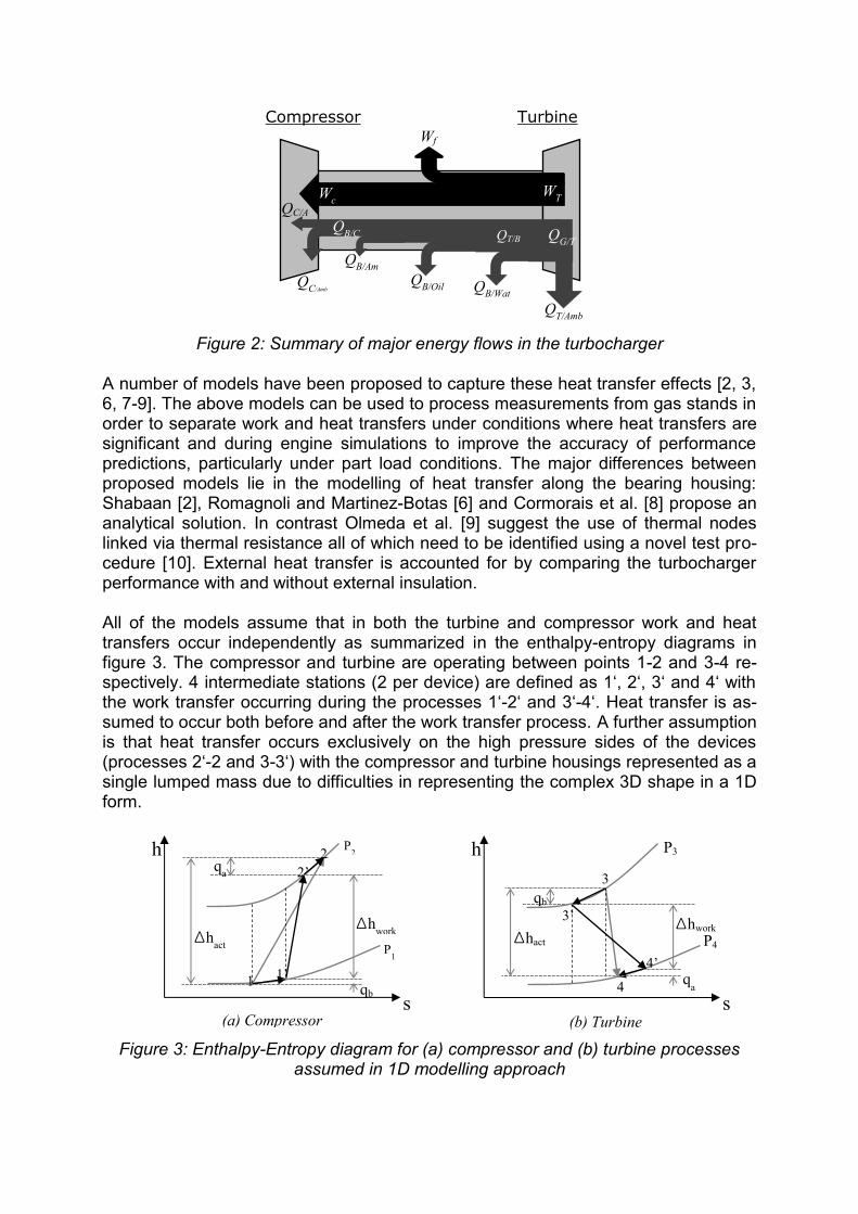
Figure 2: Summary of major energy flows in the turbocharger

A number of models have been proposed to capture these heat transfer effects [2, 3, 6, 7-9]. The above models can be used to process measurements from gas stands in order to separate work and heat transfers under conditions where heat transfers are significant and during engine simulations to improve the accuracy of performance predictions, particularly under part load conditions. The major differences between proposed models lie in the modelling of heat transfer along the bearing housing: Shabaan [2], Romagnoli and Martinez-Botas [6] and Cormorais et al. [8] propose an analytical solution. In contrast Olmeda et al. [9] suggest the use of thermal nodes linked via thermal resistance all of which need to be identified using a novel test pro-cedure [10]. External heat transfer is accounted for by comparing the turbocharger performance with and without external insulation. All of the models assume that in both the turbine and compressor work and heat transfers occur independently as summarized in the enthalpy-entropy diagrams in figure 3. The compressor and turbine are operating between points 1-2 and 3-4 re-spectively. 4 intermediate stations (2 per device) are defined as 1‘, 2‘, 3‘ and 4‘ with the work transfer occurring during the processes 1‘-2‘ and 3‘-4‘. Heat transfer is as-sumed to occur both before and after the work transfer process. A further assumption is that heat transfer occurs exclusively on the high pressure sides of the devices (processes 2‘-2 and 3-3‘) with the compressor and turbine housings represented as a single lumped mass due to difficulties in representing the complex 3D shape in a 1D form.

Figure 3: Enthalpy-Entropy diagram for (a) compressor and (b) turbine processes

assumed in 1D modelling approach

Compressor

h

s

P4

P3

Wf

qb

Wc

qa

WT

Δhact

QT/Amb

Δhwork

QB/Am

b

h

QB/Oil

s

QC/Amb

Turbine

P1

QB/Wat

P2

qa

QG/T

qb

QB/C

Δhact

QC/A

Δhwork

QT/B

(a) Compressor (b) Turbine

1 1’

2 2’

4 4’

3’

3

There have been limited published works on 3D simulation studies into the heat transfer effects in turbochargers. Bohn et al. [11] undertook such a study and simu-lated the complete compression process for a range of conditions. Their work fo-cussed on intake gas flow from the compressor intake, through the impeller and into the diffuser however crucially did not present results from the volute which all influ-ences the gas temperature at the exit of the compressor. Their results showed that the heat transfer before compression could be significant depending on the operating conditions and is always a flow of heat towards the gas, thus raising its temperature. Heat transfer after the compression processes depended on whether the tempera-ture rise was sufficient to raise the temperature above that of the housing which is more a function of pressure ratio that mass flow rate. However, it is not clear as to the significant of this heat flow when heat transfer in the volute is also included. This paper will focus on this assumption within the compressor and assess the validi-ty of a single mass representing the compressor housing and the assumption of heat transfer only occurring after the compression process.

3. Methodology This work combines a 3D conjugate heat transfer study with a 1D heat transfer mod-el. The 3D model shows detailed heat flows inside the compressor housing and fluid in a way that can advise the simplifications for 1D modelling of the compressor hous-ing. 3.1 Turbocharger The turbocharger used in this study was from a 2.2L automotive Diesel engine, with turbine and compressor wheel diameters of 43mm and 49mm respectively. The tur-bine side included variable guide vanes and lubricating oil for the journal bearing sys-tem also provides a level of cooling for the device. The device has been fully mod-elled in 1D and a detailed 3D conjugate heat transfer analysis of the compressor has been performed. 3.2 Heat transfer modelling 3.2.1 One-Dimensional Heat Transfer Model A one dimensional heat transfer model of a turbocharger has been developed which simulated the turbocharger along with a compressor back-pressure valve. The model is based on those found in the literature and described in section 2.2 above and a detailed presentation of this model can be found in [7]. The model is based on com-pressor and turbine maps. The model set point is controlled by defining the following parameters:

- Turbine inlet and outlet pressures - Turbine inlet temperature - Compressor inlet pressure and temperature

The compressor outlet pressure is calculated through a backpressure valve sub model which, with the compressor model, balances the flow of gas into and out of an intermediate volume. The opening of this valve is also a model input. The map based model is combined with a heat transfer sub model: convective heat transfer within the compressor housing is modelled using equation 5

𝑄𝑇𝑜𝑡𝑎𝑙 = 𝑄𝑏 + 𝑄𝑎 = ℎ𝑏𝐴𝑏(𝑇1 − 𝑇𝑐) + ℎ𝑎𝐴𝑎(𝑇2′ − 𝑇𝑐) (5)

The convective heat transfer coefficient is derived from a relationship based on the Seider-Tate correlation for flows in pipes [12] (equation 6) and in this work it is as-sumed that this correlation is the same both before and after compression, with only changes in Reynolds and Nusselt numbers due to changes in the effective geometry.

𝑁𝑢𝑑 = 𝑎1𝑅𝑒𝑑𝑎2𝑃𝑟𝑎3 (

𝜇𝑏𝑢𝑙𝑘

𝜇𝑠𝑘𝑖𝑛)

𝑎4

(6)

Of importance in this work is the treatment of the heat transfer between the intake air and the compressor housing node. The model assumes a single thermal mass rep-resenting the complete compressor housing (i.e. the conductivity of the housing itself is negligible). The compressor housing is linked to the bearing housing and heat is transferred between these two components via conduction. The outer surface of the housing is exposed to ambient air whilst the inner surface is exposed to the intake air flow [7]. It is assumed that a proportion of the internal surface will be exposed to the intake gas before it is compressed, at a temperature close to ambient; the remainder of the internal area will be exposed to the gas after compression, at a higher temper-ature dependent on the compression ratio and isentropic efficiency of the compressor at the particular operating point. This breakdown in internal area will be controlled by

a parameter 𝛼𝐴 defined in equation 7.

𝐴𝑇 = 𝐴𝑏 + 𝐴𝑎 = 𝛼𝐴𝐴𝑇 + (1 − 𝛼𝐴)𝐴𝑇 (7)

As calculation time is less important for the 1D model which converges much faster than the 3D model, simulations were conducted along of the compressor speed lines for five different compressor back pressure valve openings ranging from near the surge line to choke conditions as shown in figure 4 (total of 20 test points per operat-ing map). For each test point the compressor back pressure valve was controlled to give a desired compressor mass flow whilst the turbine inlet pressure was adjusted to give the desired target shaft speed. Each of the test points was simulated with four different conditions of TIT: 100oC, 300oC, 500oC and adiabatic. For adiabatic test conditions, external heat transfer model was disabled to simulate the effect of thermal insulation whilst the turbine inlet temperature and oil temperature were set to be the same as the compressor outlet temperature. For all other conditions external heat transfer was modelled, oil temper-ature was simulated at 100oC. For each of the test conditions considered above, four different distributions of internal heat transfer area were simulated: αA=0, αA=0.1, αA=0.2 and αA=0.3 in equation 7 such that overall 16 different compressor maps were produced. This can be interpreted as 0%, 10%, 20% and 30% of internal surface be-ing exposed to low temperature intake air before compression.

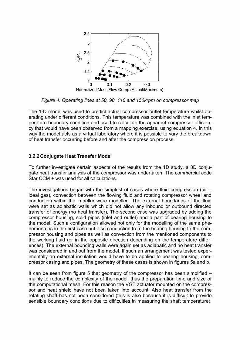
Figure 4: Operating lines at 50, 90, 110 and 150krpm on compressor map

The 1-D model was used to predict actual compressor outlet temperature whilst op-erating under different conditions. This temperature was combined with the inlet tem-perature boundary condition and used to calculate the apparent compressor efficien-cy that would have been observed from a mapping exercise, using equation 4. In this way the model acts as a virtual laboratory where it is possible to vary the breakdown of heat transfer occurring before and after the compression process. 3.2.2 Conjugate Heat Transfer Model To further investigate certain aspects of the results from the 1D study, a 3D conju-gate heat transfer analysis of the compressor was undertaken. The commercial code Star CCM + was used for all calculations. The investigations began with the simplest of cases where fluid compression (air – ideal gas), convection between the flowing fluid and rotating compressor wheel and conduction within the impeller were modelled. The external boundaries of the fluid were set as adiabatic walls which did not allow any inbound or outbound directed transfer of energy (no heat transfer). The second case was upgraded by adding the compressor housing, solid pipes (inlet and outlet) and a part of bearing housing to the model. Such a configuration allowed not only for the modelling of the same phe-nomena as in the first case but also conduction from the bearing housing to the com-pressor housing and pipes as well as convection from the mentioned components to the working fluid (or in the opposite direction depending on the temperature differ-ences). The external bounding walls were again set as adiabatic and no heat transfer was considered in and out from the model. If such an arrangement was tested exper-imentally an external insulation would have to be applied to bearing housing, com-pressor casing and pipes. The geometry of these cases is shown in figures 5a and b. It can be seen from figure 5 that geometry of the compressor has been simplified – mainly to reduce the complexity of the model, thus the preparation time and size of the computational mesh. For this reason the VGT actuator mounted on the compres-sor and heat shield have not been taken into account. Also heat transfer from the rotating shaft has not been considered (this is also because it is difficult to provide sensible boundary conditions due to difficulties in measuring the shaft temperature).

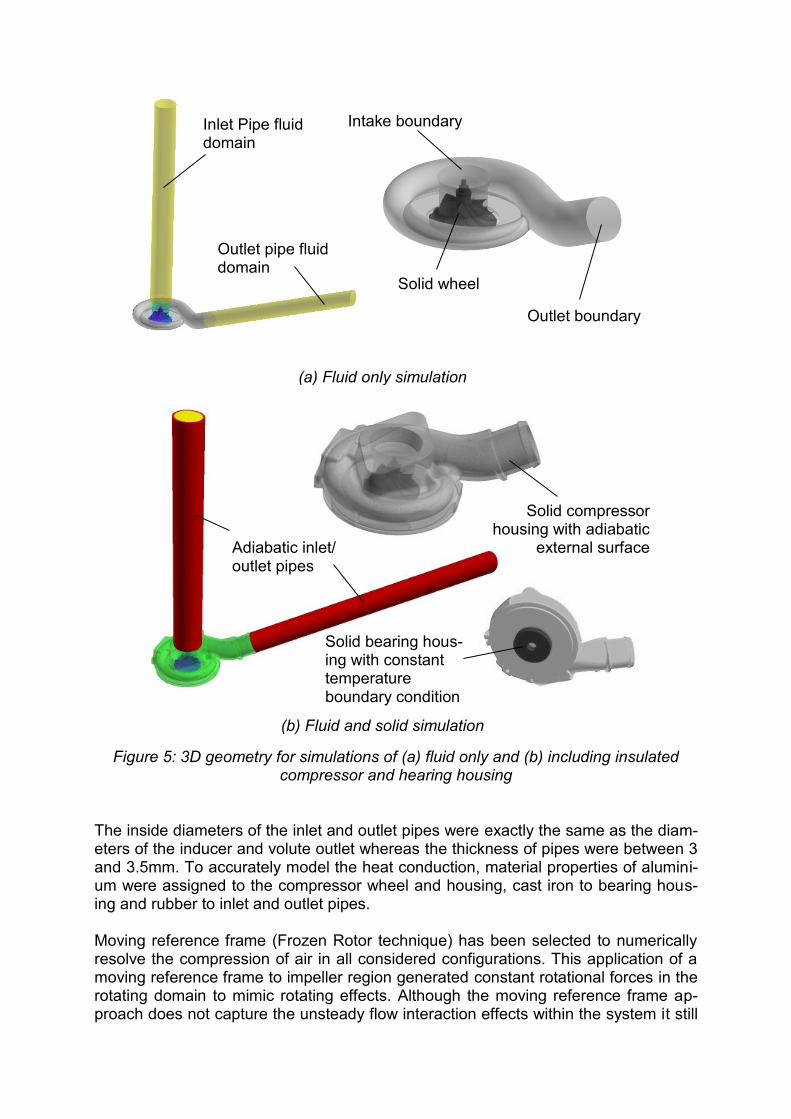
Figure 5: 3D geometry for simulations of (a) fluid only and (b) including insulated compressor and hearing housing

The inside diameters of the inlet and outlet pipes were exactly the same as the diam-eters of the inducer and volute outlet whereas the thickness of pipes were between 3 and 3.5mm. To accurately model the heat conduction, material properties of alumini-um were assigned to the compressor wheel and housing, cast iron to bearing hous-ing and rubber to inlet and outlet pipes. Moving reference frame (Frozen Rotor technique) has been selected to numerically resolve the compression of air in all considered configurations. This application of a moving reference frame to impeller region generated constant rotational forces in the rotating domain to mimic rotating effects. Although the moving reference frame ap-proach does not capture the unsteady flow interaction effects within the system it still

Inlet Pipe fluid domain

Outlet pipe fluid domain

Solid wheel

Outlet boundary

Intake boundary

(a) Fluid only simulation

(b) Fluid and solid simulation

Solid bearing hous-ing with constant temperature boundary condition

Solid compressor housing with adiabatic

external surface Adiabatic inlet/ outlet pipes

seemed appropriate to cover the steady-state nature of the phenomena under con-sideration – both investigated operating points were selected from stable area of the compressor performance map (away from surge and choke lines). Before the simula-tions were run, all solid regions had an initial temperature set to 298K. The evaluation of the 3D CFD compression prediction was based on the comparison of simulated total pressure and temperature at volute exit (mass flow averaged) with the values taken from the compressor performance map interpolation process. To resolve the compression of the flowing air the following boundary conditions have been chosen:

- Atmospheric pressure and static temperature at the fluid inlet boundary - Compressor impeller rotational speed - Air mass flow rate at the volute outlet

The conductive heat transfer within the solids was driven by the temperature differ-ences of the working fluid and external surfaces of the bearing housing. The sum-mary of boundary conditions and results for simulated cases can found in section 4.2.

The numerical mesh was constructed from polyhedral elements throughout all do-mains with additional prism layers on all external fluid boundaries to enhance the predictions in boundary layer. The adjacent mesh of the solid regions was also en-hanced with prisms to improve the heat transfer modelling between fluid and solid phases. The first investigated case numerical model was built from 1.78mln grid cells whereas the second from 3.55mln. Standard RANS K-є turbulence model has been chosen for all simulations.

4. Results

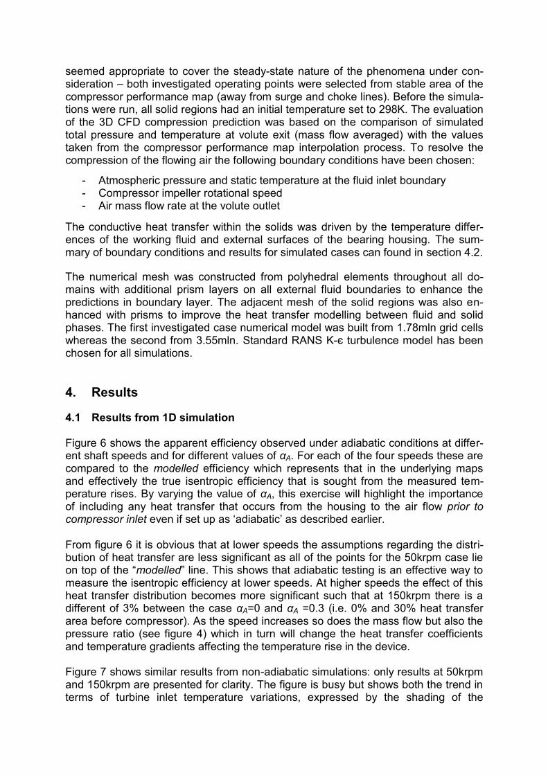
4.1 Results from 1D simulation Figure 6 shows the apparent efficiency observed under adiabatic conditions at differ-ent shaft speeds and for different values of αA. For each of the four speeds these are compared to the modelled efficiency which represents that in the underlying maps and effectively the true isentropic efficiency that is sought from the measured tem-perature rises. By varying the value of αA, this exercise will highlight the importance of including any heat transfer that occurs from the housing to the air flow prior to compressor inlet even if set up as ‘adiabatic’ as described earlier. From figure 6 it is obvious that at lower speeds the assumptions regarding the distri-bution of heat transfer are less significant as all of the points for the 50krpm case lie on top of the “modelled” line. This shows that adiabatic testing is an effective way to measure the isentropic efficiency at lower speeds. At higher speeds the effect of this heat transfer distribution becomes more significant such that at 150krpm there is a different of 3% between the case αA=0 and αA =0.3 (i.e. 0% and 30% heat transfer area before compressor). As the speed increases so does the mass flow but also the pressure ratio (see figure 4) which in turn will change the heat transfer coefficients and temperature gradients affecting the temperature rise in the device. Figure 7 shows similar results from non-adiabatic simulations: only results at 50krpm and 150krpm are presented for clarity. The figure is busy but shows both the trend in terms of turbine inlet temperature variations, expressed by the shading of the

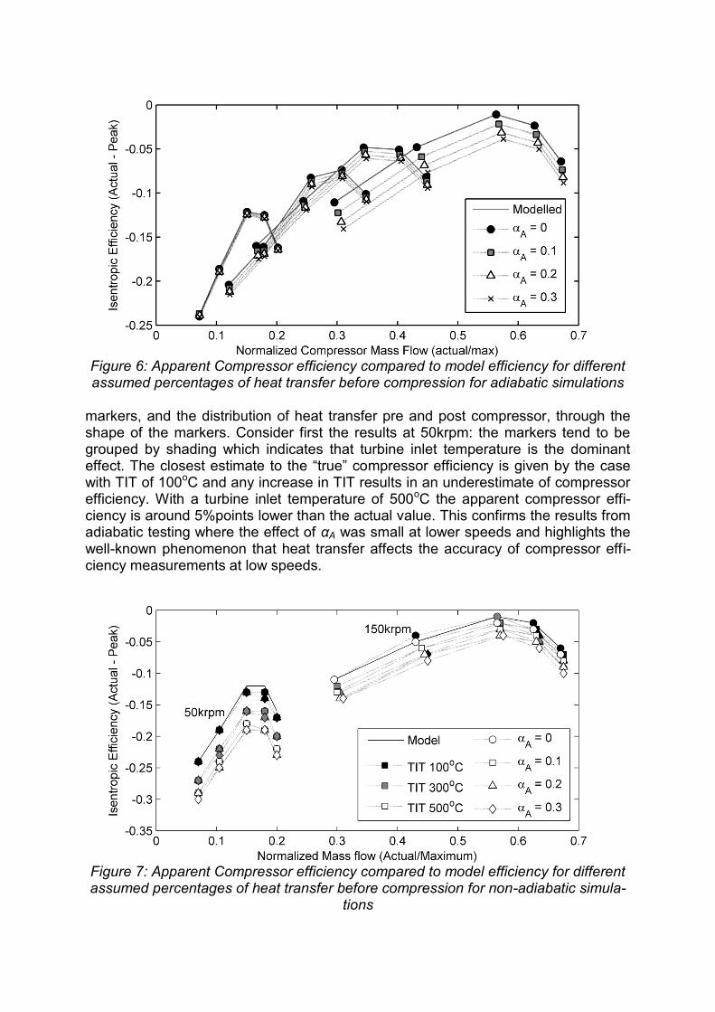
Figure 6: Apparent Compressor efficiency compared to model efficiency for different assumed percentages of heat transfer before compression for adiabatic simulations

markers, and the distribution of heat transfer pre and post compressor, through the shape of the markers. Consider first the results at 50krpm: the markers tend to be grouped by shading which indicates that turbine inlet temperature is the dominant effect. The closest estimate to the “true” compressor efficiency is given by the case with TIT of 100oC and any increase in TIT results in an underestimate of compressor efficiency. With a turbine inlet temperature of 500oC the apparent compressor effi-ciency is around 5%points lower than the actual value. This confirms the results from adiabatic testing where the effect of αA was small at lower speeds and highlights the well-known phenomenon that heat transfer affects the accuracy of compressor effi-ciency measurements at low speeds.

Figure 7: Apparent Compressor efficiency compared to model efficiency for different assumed percentages of heat transfer before compression for non-adiabatic simula-

tions

(a) Adiabatic (b) TIT 100oC

(c) TIT 300oC (d) TIT 500oC

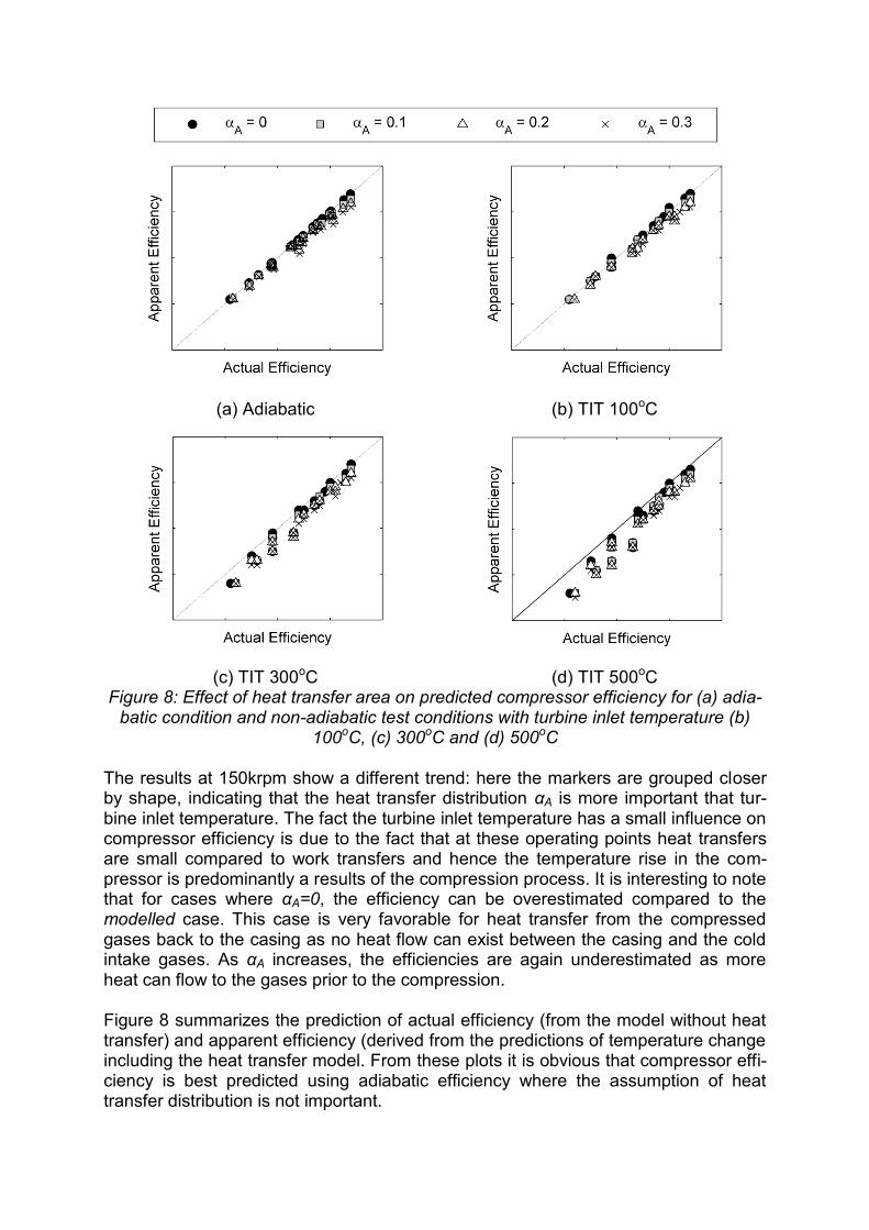
Figure 8: Effect of heat transfer area on predicted compressor efficiency for (a) adia-batic condition and non-adiabatic test conditions with turbine inlet temperature (b)

100oC, (c) 300oC and (d) 500oC The results at 150krpm show a different trend: here the markers are grouped closer by shape, indicating that the heat transfer distribution αA is more important that tur-bine inlet temperature. The fact the turbine inlet temperature has a small influence on compressor efficiency is due to the fact that at these operating points heat transfers are small compared to work transfers and hence the temperature rise in the com-pressor is predominantly a results of the compression process. It is interesting to note that for cases where αA=0, the efficiency can be overestimated compared to the modelled case. This case is very favorable for heat transfer from the compressed gases back to the casing as no heat flow can exist between the casing and the cold intake gases. As αA increases, the efficiencies are again underestimated as more heat can flow to the gases prior to the compression. Figure 8 summarizes the prediction of actual efficiency (from the model without heat transfer) and apparent efficiency (derived from the predictions of temperature change including the heat transfer model. From these plots it is obvious that compressor effi-ciency is best predicted using adiabatic efficiency where the assumption of heat transfer distribution is not important.

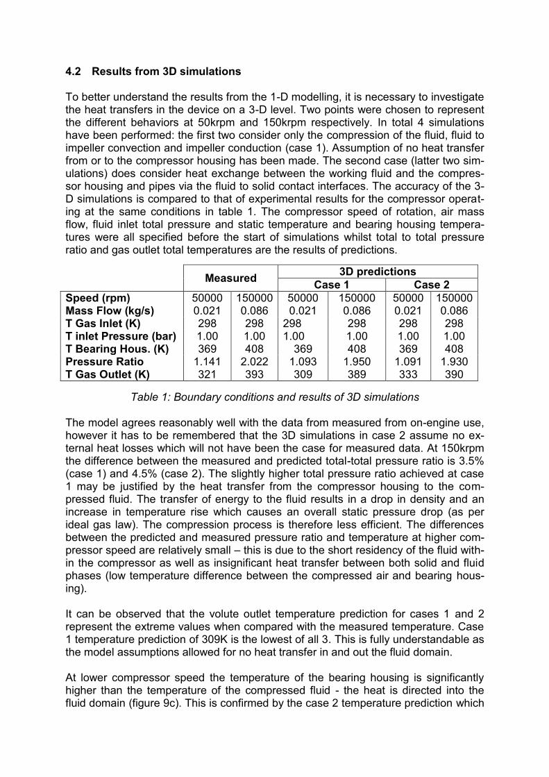
4.2 Results from 3D simulations To better understand the results from the 1-D modelling, it is necessary to investigate the heat transfers in the device on a 3-D level. Two points were chosen to represent the different behaviors at 50krpm and 150krpm respectively. In total 4 simulations have been performed: the first two consider only the compression of the fluid, fluid to impeller convection and impeller conduction (case 1). Assumption of no heat transfer from or to the compressor housing has been made. The second case (latter two sim-ulations) does consider heat exchange between the working fluid and the compres-sor housing and pipes via the fluid to solid contact interfaces. The accuracy of the 3-D simulations is compared to that of experimental results for the compressor operat-ing at the same conditions in table 1. The compressor speed of rotation, air mass flow, fluid inlet total pressure and static temperature and bearing housing tempera-tures were all specified before the start of simulations whilst total to total pressure ratio and gas outlet total temperatures are the results of predictions.

Measured

3D predictions

Case 1 Case 2

Speed (rpm) 50000 150000 50000 150000 50000 150000 Mass Flow (kg/s) 0.021 0.086 0.021 0.086 0.021 0.086 T Gas Inlet (K) 298 298 298 298 298 298 T inlet Pressure (bar) 1.00 1.00 1.00 1.00 1.00 1.00 T Bearing Hous. (K) 369 408 369 408 369 408 Pressure Ratio 1.141 2.022 1.093 1.950 1.091 1.930 T Gas Outlet (K) 321 393 309 389 333 390

Table 1: Boundary conditions and results of 3D simulations The model agrees reasonably well with the data from measured from on-engine use, however it has to be remembered that the 3D simulations in case 2 assume no ex-ternal heat losses which will not have been the case for measured data. At 150krpm the difference between the measured and predicted total-total pressure ratio is 3.5% (case 1) and 4.5% (case 2). The slightly higher total pressure ratio achieved at case 1 may be justified by the heat transfer from the compressor housing to the com-pressed fluid. The transfer of energy to the fluid results in a drop in density and an increase in temperature rise which causes an overall static pressure drop (as per ideal gas law). The compression process is therefore less efficient. The differences between the predicted and measured pressure ratio and temperature at higher com-pressor speed are relatively small – this is due to the short residency of the fluid with-in the compressor as well as insignificant heat transfer between both solid and fluid phases (low temperature difference between the compressed air and bearing hous-ing). It can be observed that the volute outlet temperature prediction for cases 1 and 2 represent the extreme values when compared with the measured temperature. Case 1 temperature prediction of 309K is the lowest of all 3. This is fully understandable as the model assumptions allowed for no heat transfer in and out the fluid domain. At lower compressor speed the temperature of the bearing housing is significantly higher than the temperature of the compressed fluid - the heat is directed into the fluid domain (figure 9c). This is confirmed by the case 2 temperature prediction which

is much higher than case 1 and significantly higher than measured one (table 1). One has to remember that in the test conditions the heat from the bearing housing is not entirely conducted through the compressor housing and then transferred to the fluid but also lost to surrounding air due to radiation and natural convection. The trend of the pressure ratio difference between cases 1 and 2 is the same as at higher com-pressor speed however both predicted values differ somewhat from the measured ones.

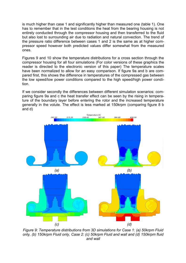
Figures 9 and 10 show the temperature distributions for a cross section through the compressor housing for all four simulations (For color versions of these graphics the reader is directed to the electronic version of this paper) The temperature scales have been normalized to allow for an easy comparison. If figure 9a and b are com-pared first, this shows the difference in temperatures of the compressed gas between the low speed/low power conditions compared to the high speed/high power condi-tion.

If we consider secondly the differences between different simulation scenarios: com-paring figure 9a and c the heat transfer effect can be seen by the rising in tempera-ture of the boundary layer before entering the rotor and the increased temperature generally in the volute. The effect is less marked at 150krpm (comparing figure 8 b and d)

(a) (b)

(c) (d)

Figure 9: Temperature distributions from 3D simulations for Case 1: (a) 50krpm Fluid only, (b) 150krpm Fluid only, Case 2: (c) 50krpm Fluid and wall and (d) 150krpm fluid

and wall

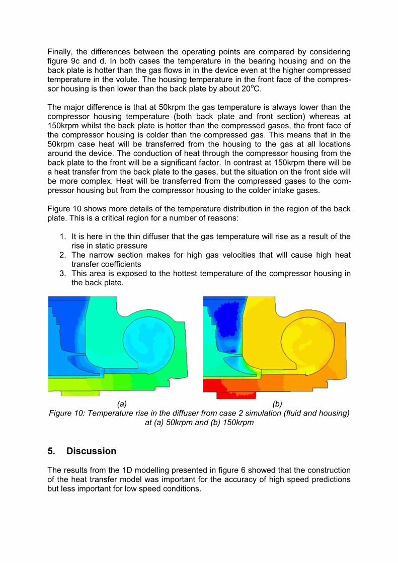
Finally, the differences between the operating points are compared by considering figure 9c and d. In both cases the temperature in the bearing housing and on the back plate is hotter than the gas flows in in the device even at the higher compressed temperature in the volute. The housing temperature in the front face of the compres-sor housing is then lower than the back plate by about 20oC. The major difference is that at 50krpm the gas temperature is always lower than the compressor housing temperature (both back plate and front section) whereas at 150krpm whilst the back plate is hotter than the compressed gases, the front face of the compressor housing is colder than the compressed gas. This means that in the 50krpm case heat will be transferred from the housing to the gas at all locations around the device. The conduction of heat through the compressor housing from the back plate to the front will be a significant factor. In contrast at 150krpm there will be a heat transfer from the back plate to the gases, but the situation on the front side will be more complex. Heat will be transferred from the compressed gases to the com-pressor housing but from the compressor housing to the colder intake gases. Figure 10 shows more details of the temperature distribution in the region of the back plate. This is a critical region for a number of reasons:

1. It is here in the thin diffuser that the gas temperature will rise as a result of the rise in static pressure

2. The narrow section makes for high gas velocities that will cause high heat transfer coefficients

3. This area is exposed to the hottest temperature of the compressor housing in the back plate.

(a) (b)

Figure 10: Temperature rise in the diffuser from case 2 simulation (fluid and housing) at (a) 50krpm and (b) 150krpm

5. Discussion The results from the 1D modelling presented in figure 6 showed that the construction of the heat transfer model was important for the accuracy of high speed predictions but less important for low speed conditions.

Results from the 3D simulation could lead us to argue to assuming a single tempera-ture for the compressor housing is not suitable for high speed conditions because it will struggle to capture the reversal of heat transfer through the compression pro-cess. At lower speeds where the heating due to compression is much less and the compressor housing temperature remains higher than the gas temperature, this is less problematic as heat flows are consistently from the housing towards the gas. A potentially more accurate model of the turbocharger heat transfers could therefore be proposed with the following modifications:

1. Allow for convective heat transfer between a node representing the compres-sor back plate and the post compression gas

2. Introducing a second thermal node representing the front face of the compres-sor housing, linked via conduction to the back plate and convection to both pre and post compression gas flows.

However the complexity of parameterizing such a model should not be underestimat-ed and the results from the 1D modelling should be considered. At the lower speed, the assumption of a single thermal node seems sufficient to significantly improve the accuracy of the turbocharger model by accounting for the heat transfers. The pro-posed new model structure could improve the accuracy at the high speed conditions, however the overall effect of heat transfer is less important in this region and it could be argued that not heat transfer model is necessary at these points.

6. Conclusions Through a combination of one and three dimensional modelling undertaken into the heat transfer in turbocharger compressors the following conclusions have been drawn:

1. One dimensional modelling showed that at low load conditions the magnitude of heat flowing to the compressor is the dominant effect causing errors in tem-perature predictions. In contrast at higher powers it is the distribution of heat transfer pre and post compression that have larger effects.

2. Heat flows in the turbocharger compressor are more complex at higher powers where the heating due to compression becomes significant and can cause the intake gases to reach a temperature higher than the compressor housing.

3. At low speeds the compressor housing remains hotter than the gases both pre and post compression and the assumption of a single lumped mass is suffi-cient to significantly improve turbocharger model accuracy.

Acknowledgements

The authors would like to thank Honeywell for supplying turbomachinery and 3D ge-ometries, their technical support and their permission to publish this work.

Abbreviations and notation Notation

𝐴 Area (m2)

𝑎1, 𝑎2 … Constants

ℎ Convective heat transfer coefficient (W/m2K)

𝐼 Shaft Inertia (kgm2)

�̇� Mass Flow (kg/s)

𝑁 Speed (rpm)

𝑁𝑢 Nusselt Number

𝑃 Pressure (Pa)

𝑃𝑅 Pressure Ratio

𝑃𝑟 Prandtl Number

𝑄 Heat (W)

𝑅𝑒 Reynolds Number

𝑇 Temperature (K)

𝑡 time (s)

𝑊 Work (W)

𝛼𝐴 Heat transfer area distribution coefficient

𝛾 Ratio of specific heats

𝜂 Isentropic Efficiency

𝜏 Torque (Nm)

𝜇𝑏𝑢𝑙𝑘 Dynamic viscority at bulk fluid temperature (Ns/m2)

𝜇𝑠𝑘𝑖𝑛 Dynamic viscosity at fluid skin temperature (Ns/m2) Subscripts 1 Pre compressor 1’ Pre compression 2 Post Compressor 2’ Post compression a After compression b Before compression c Compressor t Turbine T Turbocharger

References

[1] Cormerais, M., Hetet, J.F., Chesse, P. and Maiboom, A., Heat Transfer Analysis

in a Turbocharger Compressor: Modeling and Experiments, SAE paper Number 2006-01-0023, 2006

[2] Shaaban, S., Experimental investigation and extended simulation of turbocharger non-adiabatic performance, PhD Thesis, Universität Hannover, 2004

[3] Baines, N., K.D. Wygant, and A. Dris, The analysis of heat transfer in automotive turbochargers. Proceedings of the ASME: Journal of Engineering for Gas Turbines and Power, 132 (4), 2010

[4] Serrano, J.R., Guardiola, C., Dolz, V., Tiseira, A. and Cervello, C., Experimental Study of the Turbine Inlet Gas Temperature Influence on Turbocharger Performance, SAE paper Number 2007-01-1559, 2007

[5] Aghaali, H. and H.-E. Angstrom, Improving Turbocharged Engine Simulation by Including Heat Transfer in the Turbocharger, SAE paper Number 2012-01-0703., 2012

[6] Romagnoli, A. and R. Martinez-Botas, Heat transfer analysis in a turbocharger turbine: An experimental and computational evaluation., Applied Thermal Engineering 38(3): p. 58-77, 2012

[7] Burke, R.D., Analysis and modelling of the transient thermal behaviour og au-tomotive turbochargers, ASME Internal Combustion Engine Division Fall Con-ference 2013, Dearborn, MI, USA, 13-16 October 2013, ASME Paper Number ICEF2013-19120, 2013

[8] Cormerais, M., Chesse, P., and Hetet, J.-F., Turbocharger heat transfer model-ing under steady and transient conditions, International Journal of Thermody-namics, vol. 12, pp. 193-202, ISSN: 1301-9724, 2009

[9] Olmeda, P., Dolz, V., Arnau, F.J., and Reyes-Belmonte, M.A., Determination of heat flows inside turbochargers by means of a one dimensional lumped model, Mathematical and Computer Modelling, vol. 57, pp. 1847-1852, DOI: 10.1016/j.mcm.2011.11.078, 2013

[10] Serrano, J.R., Olmeda, P., Paez, A. and Vidal, F., An experimental procedure to determine heat transfer properties of turbochargers. Measurement Science and Technology, 21(3), , 2010

[11] Bohn, D., T. Heuer, and K. Kusterer, Conjugate flow and heat transfer investigation of a turbo charger. Proceedings of the ASME: Journal of Engineering for Gas Turbines and Power, 127(3)(3): p. 663-669, 2005

[12] Incropera, F.P. and De Witt, D.P., Introduction to Heat transfer, 2nd ed. New York: John Wiley and sons Inc., ISBN: 0-471-51728-3, 1985.

Autoren / The Authors: Dr Richard Burke , University of Bath, Bath, UK Dr Colin Copeland, University of Bath, Bath, UK Mr Tomasz Duda, University of Bath, Bath, UK