![Tribological Investigation of K Type Worm Gear Drives · Acta Polytechnica Hungarica Vol. 9, No. 6, 2012 – 233 ... Niemann [1] calculated the ... B. Magyar et al. Tribological Investigation](https://static.fdocuments.net/doc/165x107/5c3673f309d3f288708bc4e6/tribological-investigation-of-k-type-worm-gear-acta-polytechnica-hungarica-vol.jpg)
Investigation into Mechanical and Tribological Behaviour ...ethesis.nitrkl.ac.in/8000/1/675.pdf ·...
91
Investigation into Mechanical and Tribological Behaviour of Hollow Glass Microsphere (HGM) Reinforced Epoxy Composite A Thesis Submitted to National Institute of Technology, Rourkela In Partial fulfilment of the requirement for the degree of Master of Technology in Mechanical Engineering (Specialisation-Machine Design and Analysis) By Gaurav Kumar Garg (Roll No. 213ME1377) Department of Mechanical Engineering National Institute of Technology Rourkela-769008 (India) May-2015
Transcript of Investigation into Mechanical and Tribological Behaviour ...ethesis.nitrkl.ac.in/8000/1/675.pdf ·...
Investigation into Mechanical and Tribological
Behaviour of Hollow Glass Microsphere (HGM)
Reinforced Epoxy Composite
A Thesis Submitted to
National Institute of Technology, Rourkela
In Partial fulfilment of the requirement for the degree of
Master of Technology
in
Mechanical Engineering
(Specialisation-Machine Design and Analysis)
By
Gaurav Kumar Garg
(Roll No. 213ME1377)
Department of Mechanical Engineering
National Institute of Technology
Rourkela-769008 (India)
May-2015

Investigation into Mechanical and Tribological
Behaviour of Hollow Glass Microsphere (HGM)
Reinforced Epoxy Composite
A Thesis Submitted to
National Institute of Technology, Rourkela
In Partial fulfilment of the requirement for the degree of
Master of Technology
in
Mechanical Engineering
(Specialisation-Machine Design and Analysis)
By
Gaurav Kumar Garg
(Roll No. 213ME1377)
Under the guidance of
Prof. S. K. Acharya
Department of Mechanical Engineering
National Institute of Technology
Rourkela-769008 (India)
May-2015
I
National Institute of Technology
Rourkela-769008 (Orissa), INDIA
CERTIFICATE
This is to certify that the thesis entitled “INVESTIGATION INTO MECHANICAL
AND TRIBOLOGICAL PROPERTIES OF HOLLOW GLASS MICROSPHERE (HGM)
REINFORCED EPOXY COMPOSITE” submitted to the National Institute of Technology,
Rourkela by Gaurav Kumar Garg Roll No. 213ME1377 for the award of the Master of
Technology in Mechanical Engineering with specialization in Machine Design and Analysis is a
record of bonafide research work carried out by him under my supervision and guidance. The
results presented in this thesis has not been, to the best of my knowledge, submitted to any other
University or Institute for the award of any degree or diploma.
The thesis, in my opinion, has reached the standards fulfilling the requirement for
the award of Master of Technology in accordance with regulations of the Institute.
Place: Rourkela (Prof. S. K. Acharya)
Date: 26th
May, 2015 Department of Mechanical Engineering
NIT Rourkela

II
ACKNOWLEDGEMENT
It is a great pleasure to express my gratitude and indebtedness to my supervisor
Prof. S. K. Acharya for his guidance, encouragement, moral support and affection through the
course of my work.
I am also grateful to Prof. Sunil Kumar Sarangi, Director of NIT Rourkela who took
keen interest in the work. My special thanks to Prof. S.S. Mahapatra, Head of Mechanical
Engineering Department, for providing all kind of necessary facilities in the department to carry
out the experiment.
Besides my advisors, I would like to thank Mrs. Shakuntala Ojha, Mrs. Niharika
Mohanta , Ms. Soma Dalbehera and Mrs.Tanu shree berra for constant source of inspiration and
ever-cooperating attitude which empowered me in working all the initial surveys, experiments
and also to expel this thesis in the present form.
This work is also the outcome of the blessing, guidance and support of my father Mr.
Rajendra Prasad Garg & mother Mrs. Vimla Devi. This work could have been a distant dream if
I did not get the moral encouragement and help from them. This thesis is the outcome of the
sincere prayers and dedicated support of my family. And at last I am extremely thankful to all
my friends for their motivation and inspiration during this project work
Date: - 26th
May, 2015 (Gaurav Kumar Garg)
III
ABSTRACT
In the present work hollow glass microspheres (HGMs) filled epoxy composite with filler
content from 0 to 20 wt. % were prepared in order to improve the abrasive wear and mechanical
properties of epoxy. Tensile strength and impact strength were determined experimentally.
Abrasive wear test was conducted using pin-on-disc wear tester. Composites having 0, 10, 15,
and 20 weight fraction of HGM filled epoxy have been prepared in the laboratory by using a
self-designed mould. All the experiments were conducted as per ASTM standard. It was found
that as the reinforcement (HGM) increases from 0 to 20 wt. % the wear resistance as well as
mechanical properties of composite increases. The enhancement in these properties is related to
strong bonding between the HGM and epoxy which might have happened due to formation of an
interphase between the HGM and epoxy-matrix. SEM (scanned electron microscope) studies
were also carried out to know the fracture behaviour of the composite.
Keywords: HGM, Pin-on-Disc, Interphase, SEM

IV
CONTENTS
Certificate I
Acknowledgements II
Abstract III
Contents IV
List of Tables VII
List of Figures VIII
Nomenclature XI
Chapter 1 INTRODUCTION
1.1 BACKGROUND 1
1.2 TYPES OF COMPOSITES 2
1.2.1 Particulate reinforced Composites 2
1.2.2 Fibre Reinforced Composites 3
1.2.3 Structural (Laminates) Composites 3
1.3 TYPES OF COMPOSITES ACCORDING TO CLASS 4
OF MATRIX
1.3.1 Metal or Ingot matrix composites (MMC) 4
1.3.2 Ceramic or Pottery matrix composites 4
1.3.3 Organic or Polymer matrix composites 4
1.4 TYPES OF COMPOSITES ACCORDING TO CHARACTER 5
OF POLYMER
1.4.1 Thermoset (thermosetting) Polymer matrix 5
Composites
1.4.2 Thermo softening (or plastic) polymer matrix 5
Composites
1.5 BENEFITS OF POLYMER MATRIX COMPOSITES 5
1.6 DRAWBACK OF POLYMER MATRIX COMPOSITES 6

V
1.7 SCIENCE OF WEAR 6
1.8 CLASSIFICATION OF WEAR 7
1.8.1 Surface Fatigue Wear 7
1.8.2 Corrosive Wear 7
1.8.3 Abrasive Wear 7
1.8.4 Adhesive Wear 8
1.8.5 Erosion Wear 9
1.9 INTODUCTION TO POLYMER COMPOSITE WITH 9
HOLLOW GLASS MICROSPHERE (HGM)
1.3.1 Introduction to Hollow Glass Microsphere 9
1.3.2 Introduction of Epoxy as a polymer matrix 11
2.0 DEMONSTRATION OF RESEARCH TOPIC 11
Chapter 2 LITERATURE REVIEW
2.1 LITERATURE REVIEW 12
2.2 LITERATURE SURVEY ON MATRIX MATERIAL 12
2.3 LITERATURE SURVEY ON HOLLOW GLASS 13
MICROSPHERE
Chapter 3 MECHANICAL TESTING OF HOLLOW GLASS
MICROSPHERE REINFORCED EPOXY COMPOSITE
3.1 MATERIAL USED 17
3.1.1 Hollow Glass Microsphere (HGM) 17
3.1.2 Epoxy Resin 18
3.1.3 Hardener 19
3.2 EXPERIMENTAL DETAILS 19
3.2.1 Sample Preparation 19
3.3 CHARACTERIZATION OF COMPOSITES 20
3.3.1 Density Measurement 20
3.3.2 Void Content 20
3.3.3 XRD (X-Ray Diffraction) Analysis 21
VI
3.4 TESTING OF MECHANICAL PROPERTIES OF COMPOSITES
3.4.1 Tensile Test 23
3.4.2 Impact Test 24
3.5 RESULTS AND DISCUSSION 26
3.6.1 Effect of filler concentration on tensile strength 26
of composite
3.6.2 Effect of filler concentration on impact strength 27
of composite
Chapter 4 DRY SLIDING ABRASIVE WEAR TESTING OF HOLLOW GLASS
MICRO SPHERE (HGM) FILLED EPOXY COMPOSITE
4.1 INTRODUCTION 28
4.2 EXPERIMENTAL DETAILS 28
4.2.1 Composite fabrication 28
4.2.2 Dry Sliding Wear Test 30
4.2.3 Calculation of Wear 31
4.3 SEM (Scanning Electron Microscope) Morphology 62
4.4 RESULTS AND DISCUSSION 64
Chapter 5 CONCLUSION AND FUTURE WORK
5.1 CONCLUSION 66
5.2 FUTURE WORK 67
REFERENCES 68

VII
List of Tables
Table No. Title Page No.
3.1 Chemical composition of borosilicate glass 17
3.2 Properties of Hollow Glass Microsphere according 18
to 3M
3.3 Tensile characteristics of HGM filled epoxy composite 24
3.4 Impact characteristics of HGM filled epoxy composite 25
4.1 Test Parameter for dry sliding abrasion wear test 33
4.2 Density of different samples 33
4.3 to 4.37 Weight loss (Δm), Wear rate (W ), Volumetric wear rate 34
(Wv) and Specific wear rate (Ws) of tested composite
samples for different weight fraction of bagasse
composite for different Sliding velocities and Sliding
distances

VIII
List of Figures
Figure No. Title Page No.
1.1 Schematic representations of Abrasion wear 8
1.2 Schematic representations of Adhesive wear 8
1.3 Schematic representations of Erosive wear 9
1.4 (a) Schematic representations of HGM particles 10
1.4 (b) Microscopic view of HGM particles 10
1.5 Chemical Structure of DGEBA 11
3.1 Hand Lay-up set up 20
3.2 Mould used for making composite 20
3.3 Specimen after fabrication 20
3.4 Intensity Variation with diffraction angle 22
3.5 Dog bone shape of the tensile testing sample 23
3.6 (a) UTM Machine Sample holder 23
3.6 (b) UTM Machine Sample loaded 23
3.7 Dimension of impact test specimen 24
3.8 Pictographic view of Impact tester 25
3.9 Effect of hollow glass microsphere content on 26
tensile strength of composite
3.10 Effect of hollow glass microsphere content on 27
tensile strength of composite
4.1 Mould used for preparing samples 29
4.2 Two halves of the mould 29
4.3 Fabricated Composite pins 29
4.4 Pin-on-disc machine 30
4.5 Fabricated Pin under abrasion testing 30
4.6 Variation of abrasive wear rate with sliding distance at 52
5N load and 200 rpm
IX
4.7 Variation of abrasive wear rate with sliding distance at 52
10N load and 200 rpm
4.8 Variation of abrasive wear rate with sliding distance at 53
15N load and 200 rpm
4.9 Variation of abrasive wear rate with sliding distance at 53
5N load and 300 rpm
4.10 Variation of abrasive wear rate with sliding distance at 54
10N load and 300 rpm
4.11 Variation of abrasive wear rate with sliding distance at 54
15N load and 300 rpm
4.12 Variation of abrasive wear rate with sliding distance at 55
5N load and 400 rpm
4.13 Variation of abrasive wear rate with sliding distance at 55
10N load and 400 rpm
4.14 Variation of abrasive wear rate with sliding distance at 56
15N load and 400 rpm
4.15 Variation of specific wear rate with sliding velocity at 56
5 N load
4.16 Variation of specific wear rate with sliding velocity at 57
10 N load
4.17 Variation of specific wear rate with sliding velocity at 57
15 N load
4.18 Variation of volumetric wear rate with load at 200 rpm 58
4.19 Variation of volumetric wear rate with load at 300 rpm 58
4.20 Variation of volumetric wear rate with load at 400 rpm 59
4.21 Variation of specific wear rate with Wt. % of filler at 5 N 59
4.22 Variation of specific wear rate with Wt. % of filler at 10 N 60
4.23 Variation of specific wear rate with Wt. % of filler at 15 N 60
4.24 Variation of coefficient of friction with load at 200 rpm 61
4.25 Variation of coefficient of friction with load at 300 rpm 61
4.26 Variation of coefficient of friction with load at 400 rpm 62
X
4.27 Abrasive surface after test (10 %10N 200 rpm) 62
4.28 (a) and (b) Abrasive surface after test (20 % 10N 300 rpm) 63
4.29 (a) and (b) Abrasive surface after test (20 % 10N 400 rpm) 63

XI
NOMENCLATURE
F Load (N)
PMCs Polymer Matrix Composites
ρ Density of the target material (gm / cm3)
Density of filler (gm / cm3)
Density of Matrix (gm / cm3)
Theoritical Density (gm / cm3)
Actual Density (gm / cm3)
∆m Weight loss (gm)
SD Sliding Distance (m)
rW Abrasive wear rate (m3/m)
sW Specific wear rate (m3/Nm)
vW Volumetric wear rate (m3/sec)
gm gram

CHAPTER 1
INTRODUCTION
1
INTRODUCTION
__________________________________________________________
1.1 BACKGROUND:
Framework is frequently marked by the materials and technology that indicate human potential
and brainpower. Cyclic work on the material was started in stone period which cause
advancement to the Copper, Iron, Steel, Aluminium and Alloy ages, as modernisation in
processing, melting took place and science made all these viable to proceed towards detecting
more beneficial materials feasible.
Composites are the material made from two or more integral materials with remarkable
dissimilar substantial or artificial features, which on joining produced a material having different
properties from original constituents. Composites materials can be a single phase or polyphase
materials which present a meaningful section of features of both phases it means by joining their
features requisite properties can be obtained.
The spectacle materials Composites having low mass to high strength ratio, inflexible and
delicate characteristics has swapped most of the metal and alloys in modern times. In current
years, polymers and their composites are rapidly substituting the traditional materials in many
engineering and systematic implications. Traditional materials have only some finite properties
with respect to combination of excessive specific modulus, specific strength and low density etc.
These materials have been used in several engineering areas beginning from space craft
implementation to industrial unit consumptions due to leading specific strength, leading
modulus, low density and improved durability [1]. In aircraft industries where strong, feather,
noncorrodible and non-breakable materials are needed and to meet alike specific requirements
the composites have to be manufactured.
2
Being featherweight, while they are the most appropriate materials for weight delicate
operations, their expensiveness limited their usage in common implementation. Use of
economical, simply achievable fillers is therefore useful to upgrade the properties and to
minimize the cost of components [2]. Compact granulated fillers including ceramic or metal bits
are being used these days to upgrade wear resistive properties of polymers [3].The injection of
such particulates into polymers for commercialized use is especially concentrate at the
minimizing price and enhancement of stiffness [4]. Many scholars [5-8] have described that the
abrading resistance of polymers upgraded by the inclusions of fillers.
1.2 Types of composites:
According to character of the matrix and filler material the composites can be categorised as
follows [9]
Particulate reinforced Composites
Big or Large Particulate
Dispersion strengthed
Fibre reinforced Composites
Continuous
Discontinuous
Structural Composites
Laminates
1.2.1 Particulate reinforced Composites:
Particle composites contain particles of one material diffuse in a matrix of a second material.
Generally the shape of particles is spherical, ellipsoidal, polyhedral, or asymmetrical in shape. In
3
this the particle is reinforced in the matrix which carry the maximum load whereas the purpose
of the reinforcement is to intercept the disorderness in the matrix due to which the plastic
distortion is difficult to occur which cause enhancement in hardness as well as tensile strength
thus inclusion of fillers refine the properties. Large bits composite is a kind of
particle-reinforced composite wherein the synergy of particle matrix cannot be considered on an
atomic or molecular stage. The level of augmentation or upgradation of mechanical action
controlled by strong bonding at the matrix-particle combination. The size of particle for
dispersion-strengthened composites, are generally minor with diameters between 0.01 - 0.1 µm
(10 - 100nm).
1.2.2 Fibre reinforced composites:
In fibre reinforced composites the diffused part is in fibre shape, generally they are used where
excessive stiffness and strength is necessary as compared to their weight. The fibre’s length is
the essential variable influencing the features of such composites. The placement and clustering
of the fibre also affects the characteristics.
1.2.3 Structural (Laminate) composites:
Laminar or Laminates composite material comes under the category of structural composites.
These types of composite materials are composed of layer of material held together by suitable
matrix. These types of composite materials have specific properties due to different layers of
composite material due to which they are able to perform a specific function. Sandwich
structures are the main type of laminar composite.

4
1.3 Types of composites according to class of matrix
Metal or Ingot matrix composites
Pottery or Ceramic matrix composites
Organic or Polymer matrix composites
1.3.1 Metal or Ingot matrix composites (MMC):
It is a composite material in which there are at least two ingredients, one exist in the form of
metal compulsory and the other can be a different ingot or an additional material such as clay or
porcelain compound. The filler material causes outstanding changes in working features of the
metal and maximum characteristics as abrading resilience, creep resilience refined. Due to these
properties it has been used in the field of aerospace such as in the rocket and space shuttle,
drilling tools, automotive disc brakes, structural parts etc.
1.3.2 Ceramic or Pottery matrix composites:
In this type of composite pottery or clay or ceramic behave as phase of matrix therefore it is
called as clay or ceramic matrix composite. They have excessive hardness and long-lasting in
contrast to traditional ceramics while maintaining the basic features such as tenuity, idleness to
synthetic response and higher- heat resistance.
1.3.2 Organic or Polymer matrix composites:
In this research work the composite used is polymer matrix composites. In organic matrix
composite the polymer is used as a matrix. Polymer is an organic or synthetically fabricated
chemical matter containing substantial molecules of numerous classes. Polymers are fabricated
by monomers which form a long chain of compound and the process is called polymerisation.
5
Polymers have light weight and high strength to weight ratio than others; it also has high
abrading resilience, due to these features they are used in flying machine and vehicle industries.
1.4 Types of composites according to character of polymer
1.4.1 Thermoset (thermosetting) Polymer matrix composites:
A thermosetting polymer which is also called thermoset is a petroleum component which
irreparable restore. The healing can be produce by high temperature, normally greater than
200 °C (392 °F), using a synthetic process, or appropriate illumination. Thermoset matrix are
generally liquids or mouldable prior to healing and are used as sealant or adhesive. Due to
consequences of that they maintain their bond formation after polymerisation. Example:
polyester, Bakelite, polyurethane, and polyepoxides (epoxy) etc.
1.4.2 Thermo softening (or plastic) polymer matrix composites:
This is a plastic material, commonly a polymer, which become mouldable beyond a certain
temperature and after cooling they become solid and preserve their shape. They comprise of
polymers that have low molecular weight and inadequate bond strength Because of these
problems thermoset polymers are better desirable in industry because they are simple during
processing and they have low cost contrast to thermo softening polymers. Examples: acrylic,
nylon, polypropene, polythene, polycarbonates.
1.5 Benefits of using polymer matrix composites:
(i) Polymer matrix composite has more tensile strength and stiffness
(ii) High abrading resistance
(iii) Cost is low compared to traditional material
6
1.6 Drawback of polymer matrix composites:
(i) Low thermal resistance
(ii) Distinguished thermal expansion coefficient
1.7 SCIENCE OF WEAR:
Wear is associated with different surface interaction and especially the displacement and
distortion of material on a work surface due to mechanical operation of the facing surface. Wear
is among the number of operation which takes place when the working surfaces of engineering
parts are loaded simultaneously and are treated with sliding, rolling and impact movement [10].
Generally wear arises through surface interactions at during relative motion, material having
harder surface may remove the loose particle from softer surface. The wear map offered by Lim
and Ashby [11] is very much helpful to determine the wear mechanism in different sliding states
moreover as the expected rates of wear. Scientists have evolved many theories in which Physical
and Mechanical properties of the materials are considered. The volume of substance decaying
over unit slide length was determined by Holm in 1940[12] from the atomic structure of wear.
The fatigue theory of wear was evolved by Kragelski [13] in 1957.evolved.This theory has been
widely accepted by scientist and researchers of various countries. Owing to the asperities in real
bodies, their meshing in sliding is different, and merging takes place at separate position which
taken in conjunction from the existent contact area. As per energy theory of wear which was
developed by Fleischer [14] in 1973 the detachment of wear particles needed that a definite
volume of material gathers a specific condemned reserve of internal energy. In all theories the
prime factor is friction.

7
1.8 CLASSIFICATION OF WEAR
Some common types of wear are classified as
Surface fatigue wear
Corrosive Wear
Rubbing or Grinding or Abrasive wear
Wear Adherent or adhesive wear
Erosion wear
1.8.1 Surface fatigue Wear:
Wear occurs due to fracture which emerge due to fatigue of material is called surface fatigue
wear. In this type of wear surface of material diminished by repeated loading.
1.8.2 Corrosive Wear:
The decline of exposed material surface due to effects of ambient air, acerbic or acids and some
volatile substances like gases etc. is known as corrosive wear. Corrosion generates cavity and
aperture and after some time it may disperse parts of the metals.
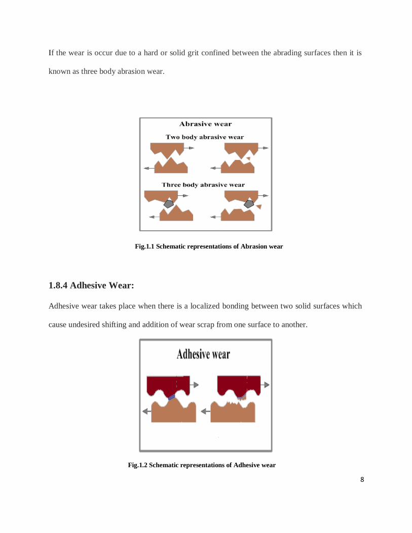
1.8.3 Abrasive Wear:
Abrasive wear will take place when there is a relative sliding motion between hard and soft
surfaces. Due to this loss of material from softer surface occur. Two body abrasions wear takes
place when hard or solid grits detach some particles from facing surface.
8
If the wear is occur due to a hard or solid grit confined between the abrading surfaces then it is
known as three body abrasion wear.
Fig.1.1 Schematic representations of Abrasion wear
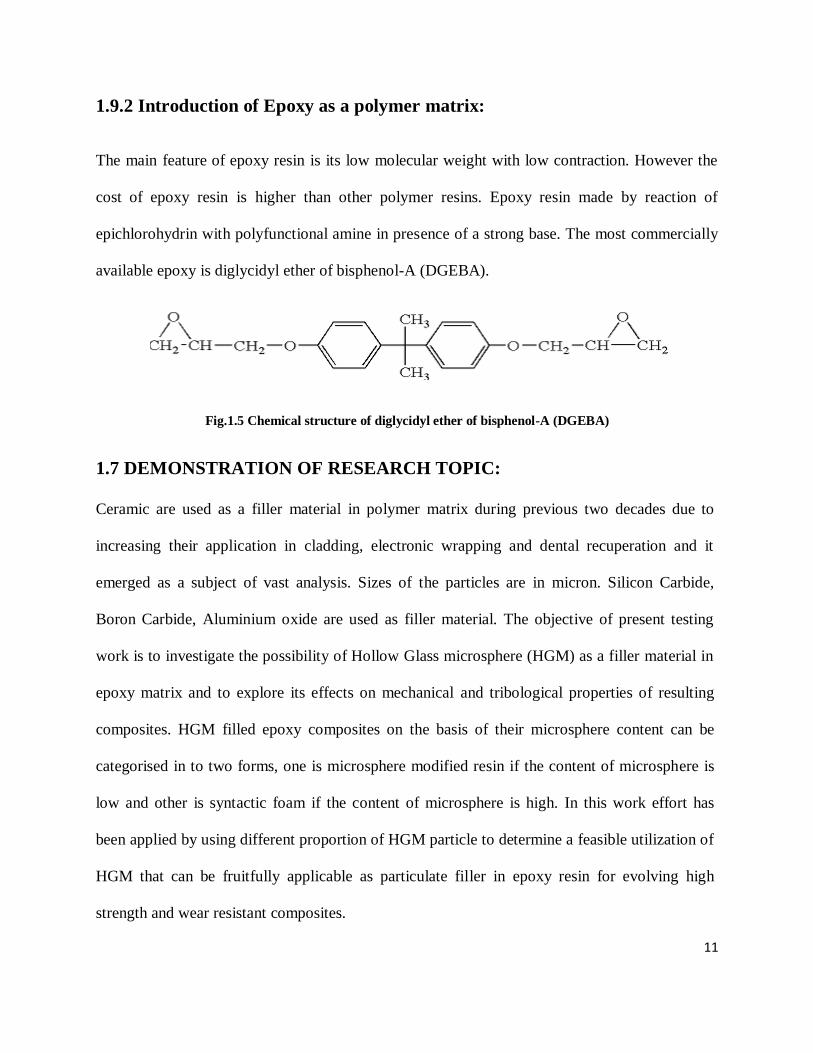
1.8.4 Adhesive Wear:
Adhesive wear takes place when there is a localized bonding between two solid surfaces which
cause undesired shifting and addition of wear scrap from one surface to another.
Fig.1.2 Schematic representations of Adhesive wear

9
1.8.5 Erosion wear:
This type of wear occurred due to impact of solid, liquid or gaseous atoms or molecules or
particles contrast to the surface of a body.
Fig.1.3 Schematic representations of Erosion wear
1.9 Introduction to Polymer composite with Hollow Glass
Microsphere (HGM):
1.9.1 Introduction to Hollow Glass Microsphere (HGM):
Hollow glass microspheres (HGMs) are solid spherical particles contain inert gas in inside
portion and stiff glass at outer portion. Sometime HGM is also called hollow glass bead or glass
bubbles or microballoons. Syntactic foam is an useful form of HGMs filled polymer composites.
HGM can be produced by inserting an inactive gas, such as argon into a constant stream of
melted glass to create discrete microspheres. The Hollow glass beads are formed by left-over or
unused material in coal depending power plants. Due to this, product commonly called as
‘cenosphere’ and conveys aluminosilicate chemistry. Small hollow glass beads are produced by
melting of silica in the coal which finally rises up in the chimneystack and spread. Glass beads or

10
spheres in the form of slag are pumped in a water mixture to the resident ash dam. Hollow
particles float on the surface of the dams while some particles which do not become hollow go
down in the ash dam. It has feather structure, enormous specific area and economical, low
dielectric constant, even flexibility and high corrosion resistance. The delicate microballoons are
chemically strong, inflammable, and unyielded and have excellent water resistance. It can be
used in coatings, putty, artificial stones etc. It can be used for emulsion explosives. Due to its
low density it can be used in oil and gas extraction industries as drilling fluid. The current
applications of syntactic foam include remotely and autonomous controlled underwater
applications, deep sea inspection, ship hulls, jet and helicopter parts, detector apparent material,
audio depletion materials, sporting goods such as bowling ball, tennis racket, soccer balls.
Microballoons made of superior optical glasses use in the area of visual resonators.
(a) (b)
Fig.1.4 (a) Schematic presentation of Hollow glass microsphere (b) Microscopic view of Hollow glass
microspheres particles
11
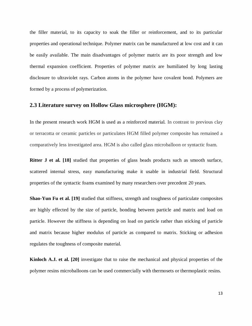
1.9.2 Introduction of Epoxy as a polymer matrix:
The main feature of epoxy resin is its low molecular weight with low contraction. However the
cost of epoxy resin is higher than other polymer resins. Epoxy resin made by reaction of
epichlorohydrin with polyfunctional amine in presence of a strong base. The most commercially
available epoxy is diglycidyl ether of bisphenol-A (DGEBA).
Fig.1.5 Chemical structure of diglycidyl ether of bisphenol-A (DGEBA)
1.7 DEMONSTRATION OF RESEARCH TOPIC:
Ceramic are used as a filler material in polymer matrix during previous two decades due to
increasing their application in cladding, electronic wrapping and dental recuperation and it
emerged as a subject of vast analysis. Sizes of the particles are in micron. Silicon Carbide,
Boron Carbide, Aluminium oxide are used as filler material. The objective of present testing
work is to investigate the possibility of Hollow Glass microsphere (HGM) as a filler material in
epoxy matrix and to explore its effects on mechanical and tribological properties of resulting
composites. HGM filled epoxy composites on the basis of their microsphere content can be
categorised in to two forms, one is microsphere modified resin if the content of microsphere is
low and other is syntactic foam if the content of microsphere is high. In this work effort has
been applied by using different proportion of HGM particle to determine a feasible utilization of
HGM that can be fruitfully applicable as particulate filler in epoxy resin for evolving high
strength and wear resistant composites.

CHAPTER 2
LITERATURE REVIEW
12
Chapter 2
__________________________________________________________
2.1 Literature Review
For an analysis of the manufacturing process, characteristics and disintegrating action of polymer
matrix composites the literature survey is an essential part of thesis. The aim of the literature
study is to make available the background data on the matter linked with current research work
and thereby to summarize the aim of the research work. Composite materials exhibit around 20%
saving over parts made from metals [15]. Due to substantial development of composite materials
in the market, problems related to need of cheapest manufacturing methods and possibilities of
reuses will have to be finding out [16].
Composite materials consist polymer as a matrix and ceramic as filler known as ceramic filled
polymer matrix composites. These types of composite materials have feather structure or light
weight, rusting resistance, wear resistance and low weight to strength ratio [9]. Due to these
features polymer matrix composite has been successfully used in vehicle and aerodynamics
industries. The behaviour of the composite materials are also effected by properties of wear i.e.
how the wear arises and what types of wear may arise etc. and the difference between the
mechanism of each wear may be examined by inspecting the working area of profile [17].
2.2 Literature survey on Matrix material:
Since it is not enough to say the matrix a dissolve paste in polymer matrix composite, it is
the massive substance which reinforced with filler material and is entirely uninterrupted. Matrix
material should be selected merely after giving cautious inspection to its chemical affinity with
13
the filler material, to its capacity to soak the filler or reinforcement, and to its particular
properties and operational technique. Polymer matrix can be manufactured at low cost and it can
be easily available. The main disadvantages of polymer matrix are its poor strength and low
thermal expansion coefficient. Properties of polymer matrix are humiliated by long lasting
disclosure to ultraviolet rays. Carbon atoms in the polymer have covalent bond. Polymers are
formed by a process of polymerization.
2.3 Literature survey on Hollow Glass microsphere (HGM):
In the present research work HGM is used as a reinforced material. In contrast to previous clay
or terracotta or ceramic particles or particulates HGM filled polymer composite has remained a
comparatively less investigated area. HGM is also called glass microballoon or syntactic foam.
Ritter J et al. [18] studied that properties of glass beads products such as smooth surface,
scattered internal stress, easy manufacturing make it usable in industrial field. Structural
properties of the syntactic foams examined by many researchers over precedent 20 years.
Shao-Yun Fu et al. [19] studied that stiffness, strength and toughness of particulate composites
are highly effected by the size of particle, bonding between particle and matrix and load on
particle. However the stiffness is depending on load on particle rather than sticking of particle
and matrix because higher modulus of particle as compared to matrix. Sticking or adhesion
regulates the toughness of composite material.
Kinloch A.J. et al. [20] investigate that to raise the mechanical and physical properties of the
polymer resins microballoons can be used commercially with thermosets or thermoplastic resins.

14
Sahu and Broutman et al. [21] investigated the fractural and mechanical behaviour of HGM
filled polyester and epoxy resins with different particulate matrices boundary conditions.
According to him glass beads are preferred as filler when the properties such as low melting
viscosity or isotropy are desired.
Broutman and Mallick et al. [22] studied the fracture, flexural and compressive characteristics
of reinforced glass powder having size of particle 15 micron with epoxy as a brittle matrix.
Ravi Kumar et al. [23] observed that compressive strength of syntactic foam for a volumetric
fraction of 0-60 % of hollow glass microsphere. According to him the compressive strength of
syntactic foam directly decreases with increase in volumetric fraction of hollow glass
microsphere. He examined that the compressive strength decrease in linear manner from 105
MPa to 25 MPa.
J.R.M. d’Almeida et al. [24] examined the effect of diameter of glass microsphere on the
mechanical performance of glass filled epoxy composite. They found that the thickness of wall
of microsphere is not related with their mean size.
S. Basavarajappa et al. [25] studied the sliding wear behaviour of composite having glass
epoxy filled with graphite and Si (silicon) particles at several loads, sliding speed and sliding
distance. According to him specific wear rate will increase directly increase of sliding velocity.
Specific wear rate was more influenced by applied load as compared to sliding velocity and
sliding distance.
K.C.Yung et al. [26] investigated the thermal properties of HGM filled epoxy composite with
volumetric content of filler in the range of 0-51.4 %. They found the improvement in thermal

15
expansion coefficient and glass transition temperature with increase in HGM content but
lowering of dielectric loss and dielectric constant of composite.
Soo – Jin Park et al. [27] examined the enhancement of mechanical interfacial and dynamic
mechanical characteristics of HGM bonded with epoxy matrix. According to him HGM filled
epoxy composites have higher free surface energy.
Ho Sung Kim et al. [28] investigated that impact behaviour of composite material can be
improve by addition of HGMs content but it will occur at the loss of flexural strength and
fracture toughness.
Jingjie Zhang et al. [29] investigated that with increase in content of broken HGMs in silicon
rubber matrix thermal conductivity, mechanical characteristics and density will improve.
Xuegang Luo et al. [30] developed the HGM filled poly butylene succinate (PBS) composite.
He tested that inclusion of HGM content (5 to 20 wt. %) enhanced the thermal stability, stiffness
and viscosity of PBS but decreased the density of composite.
Peifeng Li et al. [31] developed a three dimensional finite element model of cubic representative
elementary model (REV) to determine the failure mechanism and elastic behaviour of syntactic
foam with different volume proportion of HGM.
Jinhe wang et al. [32] observed the improvement in the mechanical characteristics such as im-
pact strength, flexural modulus and flexural strength of bisphenol a dicyanate ester with inclu-
sion of hollow glass microspheres.
16
Chang Keun Kim et al. [33] prepared a thermoplastic polyurethane grafted HGM composite
which can be used in underwater applications. According to him the tensile strength is directly
enhance with enhancement in HGM concentration whereas the density and the swelling
proportion decreased on increment of HGM concentration.
P.Li et al. [34] examined the propagation of shear ruptures at higher strain rates through
microballoons in syntactic foam which exhibited the macroscopical strain rate reliance of
compressive characteristics.
Liang and Li et al. [35, 36] studied the flexural and tensile features of acrylonitrile butadiene
styrene (ABS) filled with hollow glass bead and impact and tensile characteristics of Polyvinyl
chloride filled with hollow glass bead.
J. A. M. Ferreira et al. [37] observed the uninterrupted reduction in fatigue strength of HGM
filled epoxy composites.
CHAPTER 3
MECHANICAL TESTING OF HOLLOW
GLASS MICROSPHERE REINFORCED
EPOXY COMPOSITE
17
Chapter 3
______________________________________________
3.1 Material used:
Following materials are used in this research work
(i) Ceramic particulate ( Hollow Glass Microsphere or HGM)
(ii) Polymer Matrix (Epoxy Resin)
(iii) Hardener
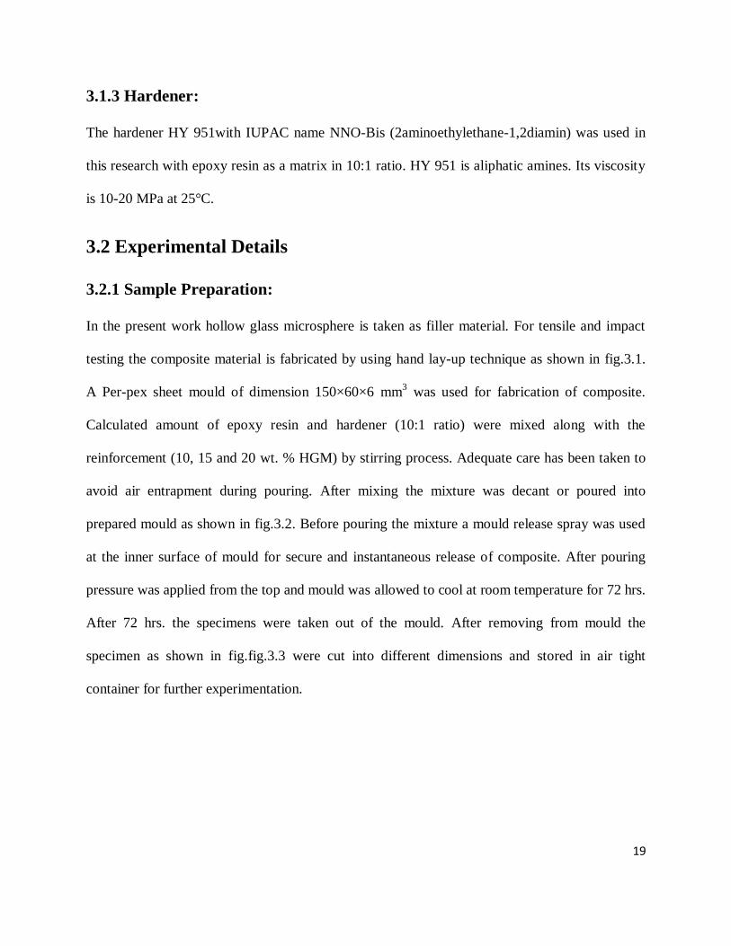
3.1.1 Hollow Glass Microsphere (HGM):
HGM used in this research is white in colour and supplied by 3M India with density 0.15 g/cc
(K15). The hollow glass microsphere used in this research is chemically stable soda lime
borosilicate glass composition having a thermal stability of 600°C. The microspheres had a wall
thickness between 10 and 30µm with particle diameters ranging from 10 to 150µm.
Table 3.1: Chemical composition of borosilicate glass
Components Wt. % Composition
SiO2 44.7
Al2O3 12.5
B2O3 14.1
CaO 26.3
Na2O 0.6
K2O 0.7

18
Table.3.2: Properties of Hollow Glass Microsphere according to 3M
Property Value
Shape Hollow, Thin Walled, Unicellular
Composition Soda-lime borosilicate
Colour White
True Density 0.15-0.60 g/cm3
Crush Strength 250-30,000 Psi
Softening Temperature 600 °C
Size 10 – 100 microns
3.1.2 Epoxy Resin:
The epoxy resin used in the current research work is araldite LY556 (bisphinol-A-diglycidyl-
ether) which is a part of epoxide group. This type of epoxy resin is supplied by CIBA GUGYE
India Limited. It has following good properties:
Dimensionally stable
Internal stress is very low
Outstanding bonding with different materials
Low contraction and Inactive to atmospheric and chemical effects
Bio-degradable, odourless, harmless, distasteful
Better electrical and mechanical properties related to other thermoset plastics
19
3.1.3 Hardener:
The hardener HY 951with IUPAC name NNO-Bis (2aminoethylethane-1,2diamin) was used in
this research with epoxy resin as a matrix in 10:1 ratio. HY 951 is aliphatic amines. Its viscosity
is 10-20 MPa at 25°C.
3.2 Experimental Details
3.2.1 Sample Preparation:
In the present work hollow glass microsphere is taken as filler material. For tensile and impact
testing the composite material is fabricated by using hand lay-up technique as shown in fig.3.1.
A Per-pex sheet mould of dimension 150×60×6 mm3 was used for fabrication of composite.
Calculated amount of epoxy resin and hardener (10:1 ratio) were mixed along with the
reinforcement (10, 15 and 20 wt. % HGM) by stirring process. Adequate care has been taken to
avoid air entrapment during pouring. After mixing the mixture was decant or poured into
prepared mould as shown in fig.3.2. Before pouring the mixture a mould release spray was used
at the inner surface of mould for secure and instantaneous release of composite. After pouring
pressure was applied from the top and mould was allowed to cool at room temperature for 72 hrs.
After 72 hrs. the specimens were taken out of the mould. After removing from mould the
specimen as shown in fig.fig.3.3 were cut into different dimensions and stored in air tight
container for further experimentation.
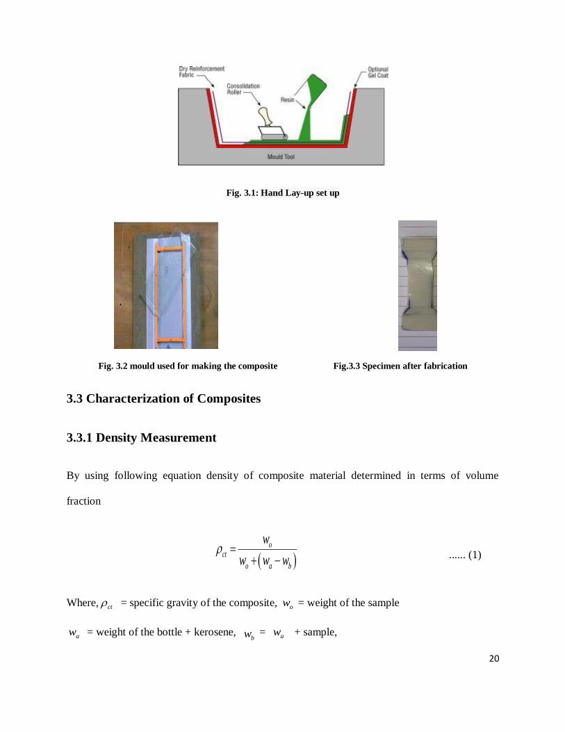
20
Fig. 3.1: Hand Lay-up set up
Fig. 3.2 mould used for making the composite Fig.3.3 Specimen after fabrication
3.3 Characterization of Composites
3.3.1 Density Measurement
By using following equation density of composite material determined in terms of volume
fraction
o
ct
o a b
w
w w w
...... (1)
Where, ct = specific gravity of the composite, ow = weight of the sample
aw = weight of the bottle + kerosene, bw = aw + sample,

21
Density of composite = ct × density of composite. In terms of weight fraction the theoretical
density of composite can be determined from formula given by Agarwal and Broutman [32]
1
ct
f m
f m
w w
...... (2)
Where w and are the weight and density correspondingly. The suffix , ,f m ct represent the
fibre, matrix and composite materials respectively
3.3.2 Void Content
According to ASTM D-2734-70 standard the void content in the composite sample can be
determined by using following expression
t a
v
t
V
...... (3)
Where, t = Theoretical Density and a = Actual Density
3.3.3 XRD (X-Ray Diffraction) Analysis
XRD is an exclusive method to find out the crystallinity (amorphous or crystalline) of composite
material, placement of particulates in specimen etc. This analysis is based on diffraction of
X-rays. When X-rays incident on the specimen then it create diffracted X-ray then different
peaks with different intensity was observed which should fulfil the Bragg’s equation i.e.
[n 2 sinn d ], where is the wavelength of X-ray radiation and is the angle of diffraction.
The measurement of the intensity and diffraction angle is helpful to find out the crystallinity of
22
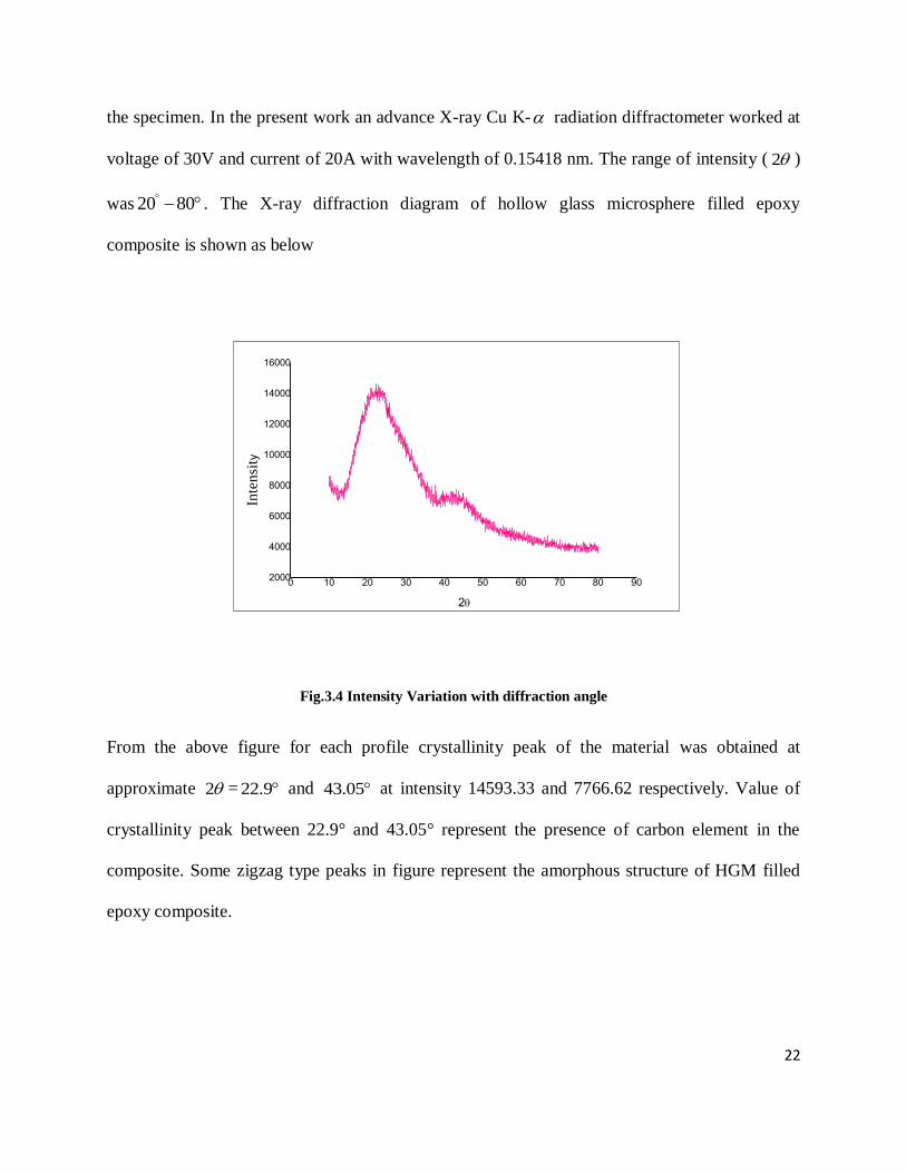
the specimen. In the present work an advance X-ray Cu K- radiation diffractometer worked at
voltage of 30V and current of 20A with wavelength of 0.15418 nm. The range of intensity ( 2 )
was 20 80 . The X-ray diffraction diagram of hollow glass microsphere filled epoxy
composite is shown as below
0 10 20 30 40 50 60 70 80 902000
4000
6000
8000
10000
12000
14000
16000
Inte
nsi
ty
2
Fig.3.4 Intensity Variation with diffraction angle
From the above figure for each profile crystallinity peak of the material was obtained at
approximate 2 = 22.9 and 43.05 at intensity 14593.33 and 7766.62 respectively. Value of
crystallinity peak between 22.9° and 43.05° represent the presence of carbon element in the
composite. Some zigzag type peaks in figure represent the amorphous structure of HGM filled
epoxy composite.
23
3.4 Testing of Mechanical Properties of Composites
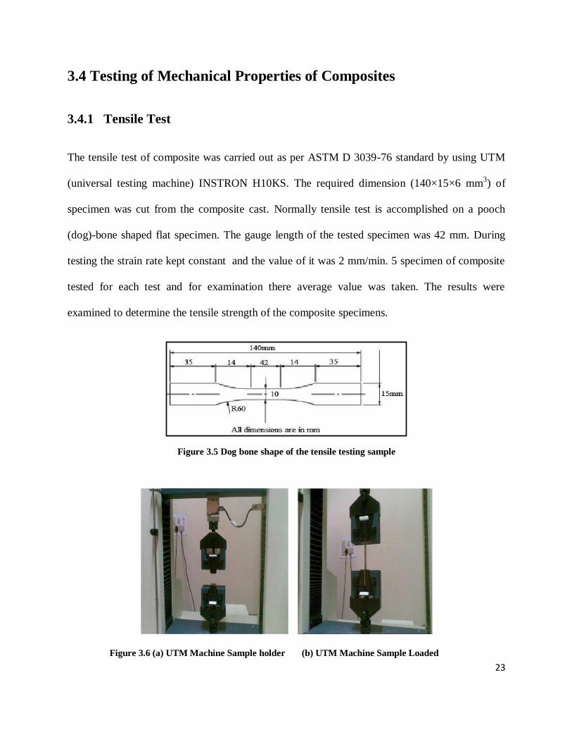
3.4.1 Tensile Test
The tensile test of composite was carried out as per ASTM D 3039-76 standard by using UTM
(universal testing machine) INSTRON H10KS. The required dimension (140×15×6 mm3) of
specimen was cut from the composite cast. Normally tensile test is accomplished on a pooch
(dog)-bone shaped flat specimen. The gauge length of the tested specimen was 42 mm. During
testing the strain rate kept constant and the value of it was 2 mm/min. 5 specimen of composite
tested for each test and for examination there average value was taken. The results were
examined to determine the tensile strength of the composite specimens.
Figure 3.5 Dog bone shape of the tensile testing sample
Figure 3.6 (a) UTM Machine Sample holder (b) UTM Machine Sample Loaded
24
Table 3.3: Tensile characteristics of HGM filled epoxy composite
Weight % of filler Tensile Strength of composite (MPa)
Pure Epoxy(0) 14.842
10 15.146
15 17.952
20 20.735
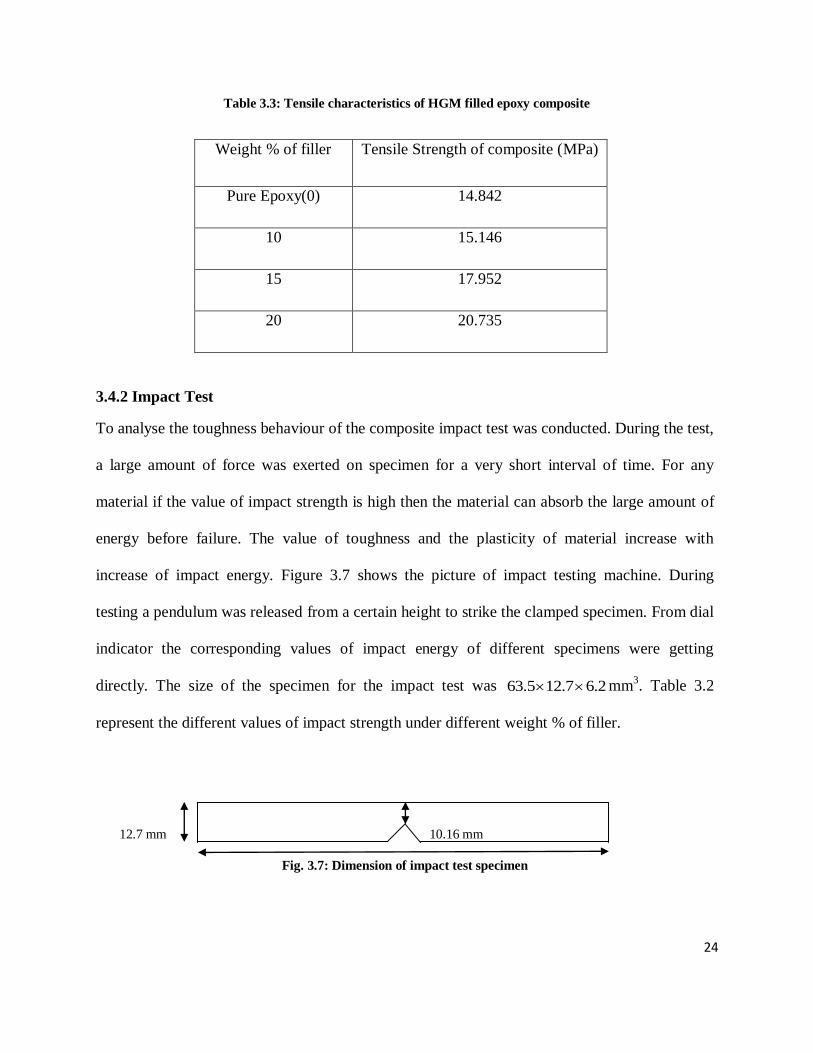
3.4.2 Impact Test
To analyse the toughness behaviour of the composite impact test was conducted. During the test,
a large amount of force was exerted on specimen for a very short interval of time. For any
material if the value of impact strength is high then the material can absorb the large amount of
energy before failure. The value of toughness and the plasticity of material increase with
increase of impact energy. Figure 3.7 shows the picture of impact testing machine. During
testing a pendulum was released from a certain height to strike the clamped specimen. From dial
indicator the corresponding values of impact energy of different specimens were getting
directly. The size of the specimen for the impact test was 63.5 12.7 6.2 mm3. Table 3.2
represent the different values of impact strength under different weight % of filler.
12.7 mm 10.16 mm
Fig. 3.7: Dimension of impact test specimen
25
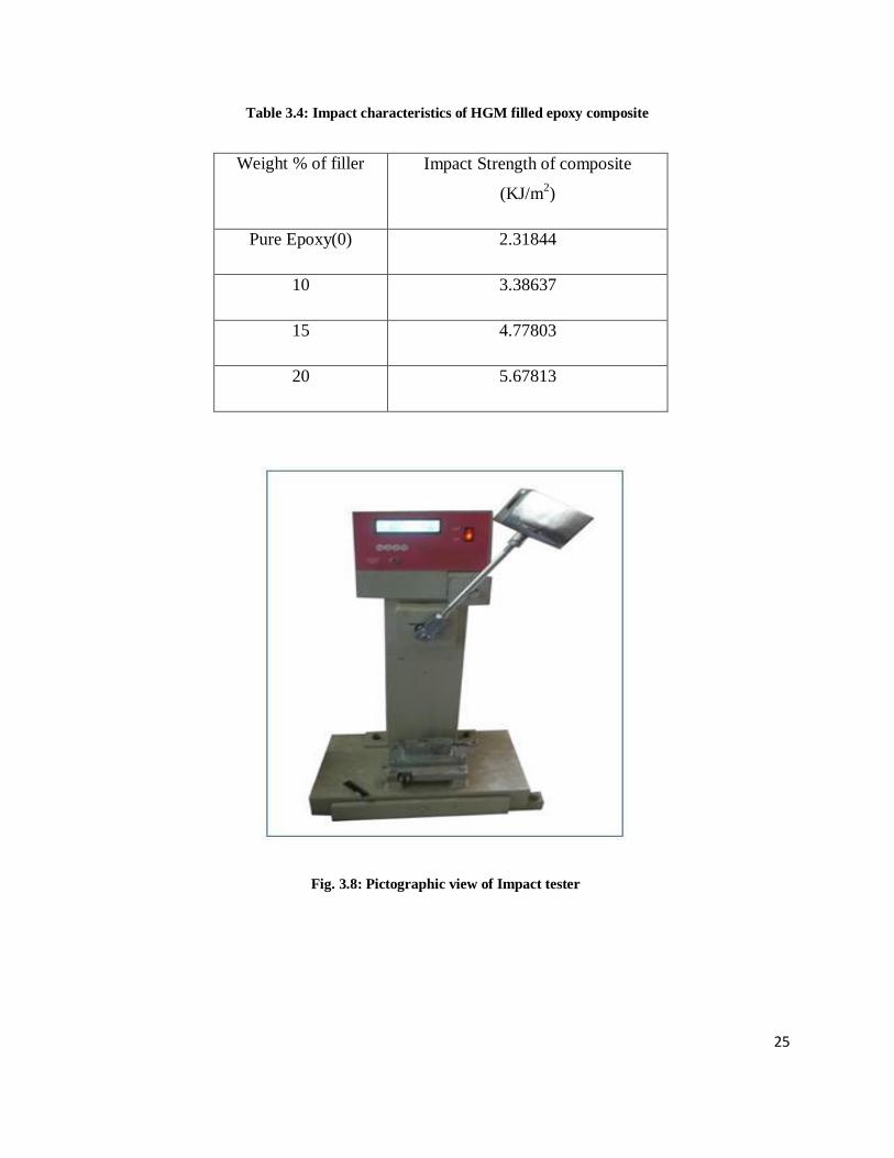
Table 3.4: Impact characteristics of HGM filled epoxy composite
Weight % of filler Impact Strength of composite
(KJ/m2)
Pure Epoxy(0) 2.31844
10 3.38637
15 4.77803
20 5.67813
Fig. 3.8: Pictographic view of Impact tester
26
3.5 RESULTS AND DISCUSSION
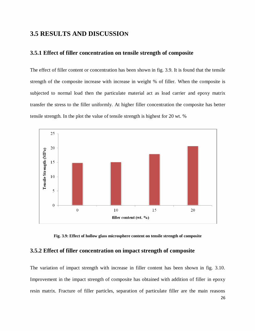
3.5.1 Effect of filler concentration on tensile strength of composite
The effect of filler content or concentration has been shown in fig. 3.9. It is found that the tensile
strength of the composite increase with increase in weight % of filler. When the composite is
subjected to normal load then the particulate material act as load carrier and epoxy matrix
transfer the stress to the filler uniformly. At higher filler concentration the composite has better
tensile strength. In the plot the value of tensile strength is highest for 20 wt. %
Fig. 3.9: Effect of hollow glass microsphere content on tensile strength of composite
3.5.2 Effect of filler concentration on impact strength of composite
The variation of impact strength with increase in filler content has been shown in fig. 3.10.
Improvement in the impact strength of composite has obtained with addition of filler in epoxy
resin matrix. Fracture of filler particles, separation of particulate filler are the main reasons

27
behind fracture of composite during impact loading. Therefore the increase in impact strength
occurs due to enhancement in applied energy. In the figure 4.4 filler content with 20 wt. %
exhibits higher impact strength. With increase in filler content in composite more energy will be
required for weakening of particulate filler matrix bonding.
Fig.3.10: Effect of hollow glass microsphere content on impact strength of composite
CHAPTER 4
DRY SLIDING ABRASIVE WEAR TESTING
OF HOLLOW GLASS MICROSPHERE
(HGM) FILLED EPOXY COMPOSITE
28
Chapter 4 __________________________________________________________
4.1 INTRODUCTION
Abrasion wear is the most intimidate wear in the industrial field which decline the life span of
expensive machine part [55]. In terms of cost this type of wear comprise 63 % of entire cost of
wear which occur when a harder surface has relative sliding motion against the softer surface
under applied load, it pierces and detach some material from the surface has low hardness which
cause cracks in the softer material. Those types of sliding parts are not failed by cracks only but
they may also failed by decline of surface due to kneading of softer surfaces against the harder
[57]. According to available literature the rate of wear caused by abrasion may vary rapidly at a
definite contact loads and sliding velocities. For attaining the development in the wear resistance
of polymer matrix composites an extensive consideration of the mechanism of abrasive wear is
required. The effects of random variables on the behaviour of abrasive wear of polymer matrix
composites can be resolved.
4.2 EXPERIMENTAL DETAILS
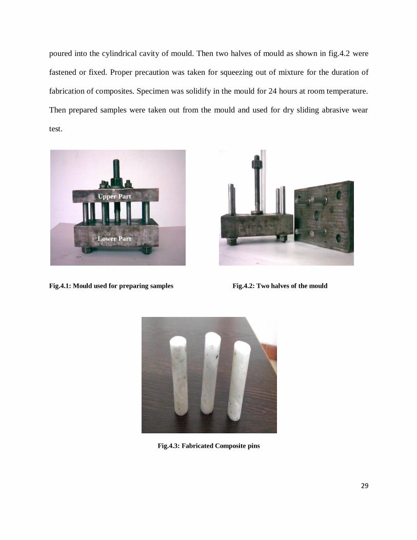
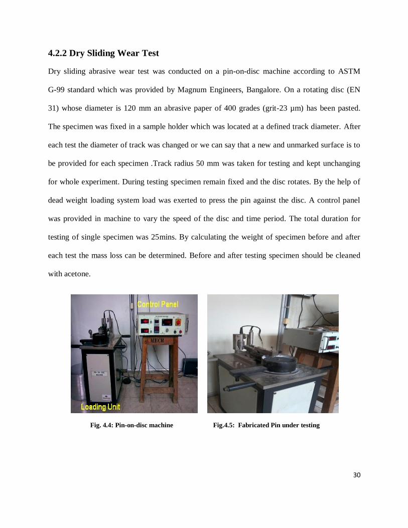
4.2.1 Composite fabrication
The particulate in a requisite amount (10, 15 and 20 wt. %) were mixed with epoxy resin along
with measured quantity of hardener. Composite specimens in cylindrical (pin) shape were
prepared in a steel mould as shown in fig.4.1. The length and diameter of specimen are 55 mm
and 10 mm respectively. The mixture of hollow glass microsphere particles and epoxy resin was
29
poured into the cylindrical cavity of mould. Then two halves of mould as shown in fig.4.2 were
fastened or fixed. Proper precaution was taken for squeezing out of mixture for the duration of
fabrication of composites. Specimen was solidify in the mould for 24 hours at room temperature.
Then prepared samples were taken out from the mould and used for dry sliding abrasive wear
test.
Fig.4.1: Mould used for preparing samples Fig.4.2: Two halves of the mould
Fig.4.3: Fabricated Composite pins
Upper Part
Lower Part
30
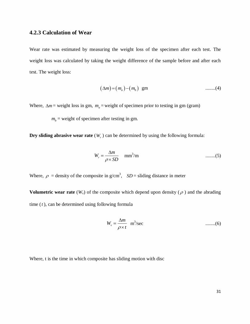
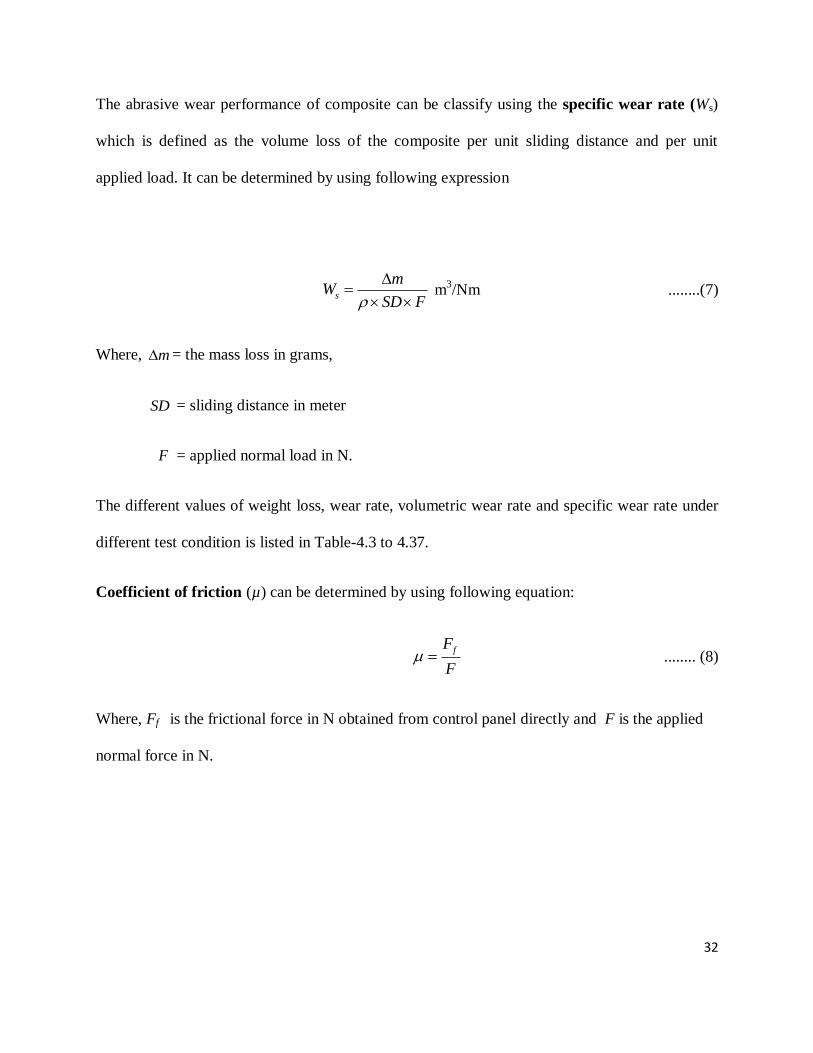
4.2.2 Dry Sliding Wear Test
Dry sliding abrasive wear test was conducted on a pin-on-disc machine according to ASTM
G-99 standard which was provided by Magnum Engineers, Bangalore. On a rotating disc (EN
31) whose diameter is 120 mm an abrasive paper of 400 grades (grit-23 µm) has been pasted.
The specimen was fixed in a sample holder which was located at a defined track diameter. After
each test the diameter of track was changed or we can say that a new and unmarked surface is to
be provided for each specimen .Track radius 50 mm was taken for testing and kept unchanging
for whole experiment. During testing specimen remain fixed and the disc rotates. By the help of
dead weight loading system load was exerted to press the pin against the disc. A control panel
was provided in machine to vary the speed of the disc and time period. The total duration for
testing of single specimen was 25mins. By calculating the weight of specimen before and after
each test the mass loss can be determined. Before and after testing specimen should be cleaned
with acetone.
Fig. 4.4: Pin-on-disc machine Fig.4.5: Fabricated Pin under testing
31
4.2.3 Calculation of Wear
Wear rate was estimated by measuring the weight loss of the specimen after each test. The
weight loss was calculated by taking the weight difference of the sample before and after each
test. The weight loss:
a bm m m gm ........(4)
Where, m = weight loss in gm, am = weight of specimen prior to testing in gm (gram)
bm = weight of specimen after testing in gm.
Dry sliding abrasive wear rate (rW ) can be determined by using the following formula:
r
mW
SD
mm
3/m ........(5)
Where, = density of the composite in g/cm3, SD = sliding distance in meter
Volumetric wear rate (Wv) of the composite which depend upon density ( ) and the abrading
time ( t ), can be determined using following formula
v
mW
t
m
3/sec ........(6)
Where, t is the time in which composite has sliding motion with disc
32
The abrasive wear performance of composite can be classify using the specific wear rate (Ws)
which is defined as the volume loss of the composite per unit sliding distance and per unit
applied load. It can be determined by using following expression
s
mW
SD F
m
3/Nm ........(7)
Where, m = the mass loss in grams,
SD = sliding distance in meter
F = applied normal load in N.
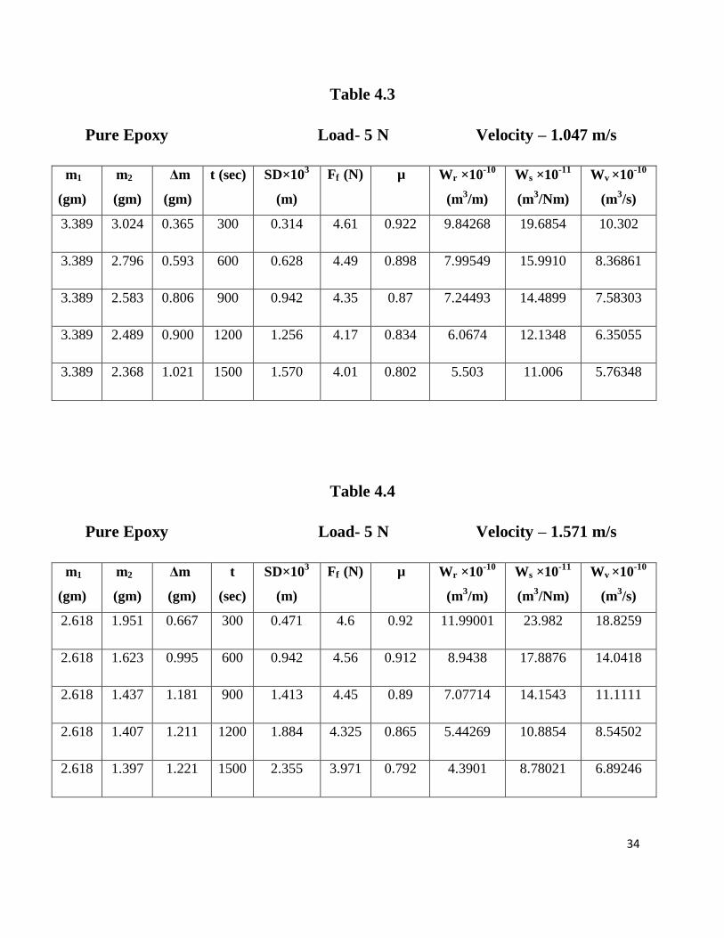
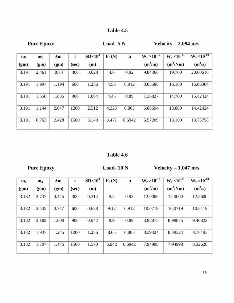
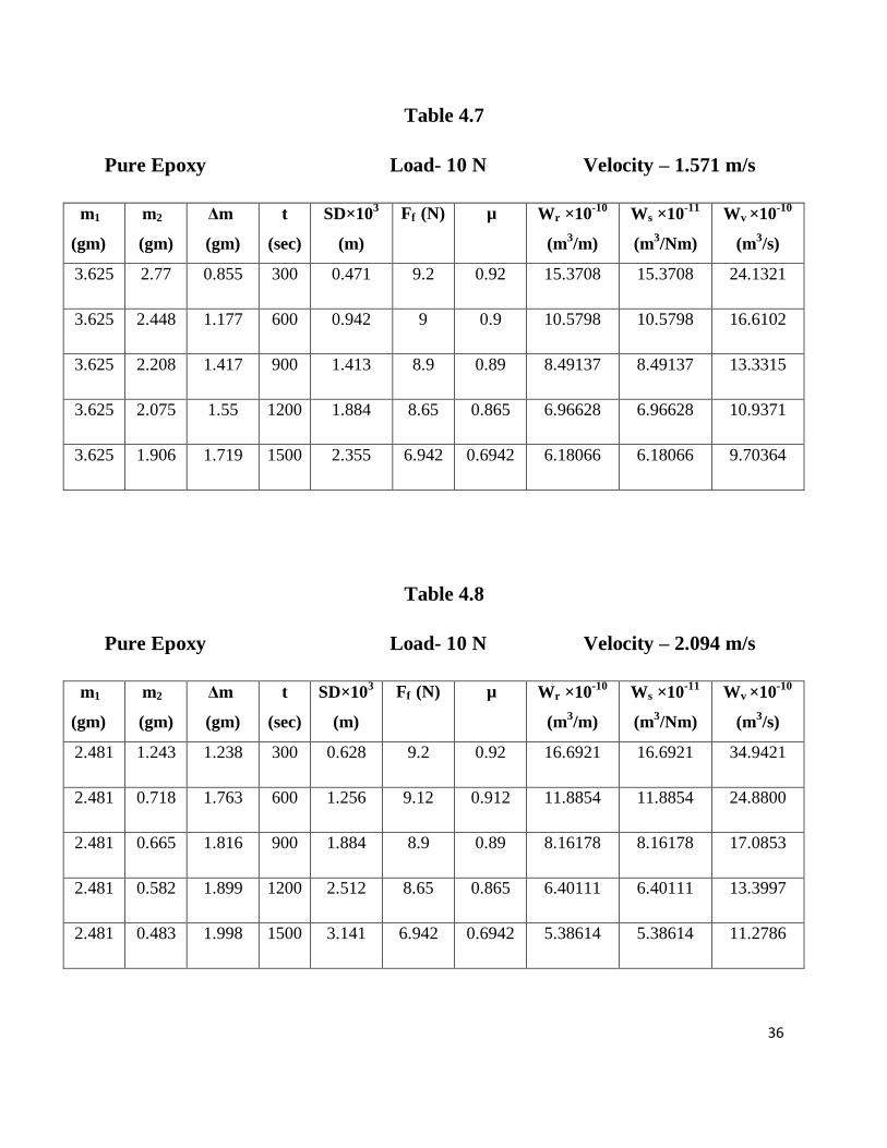
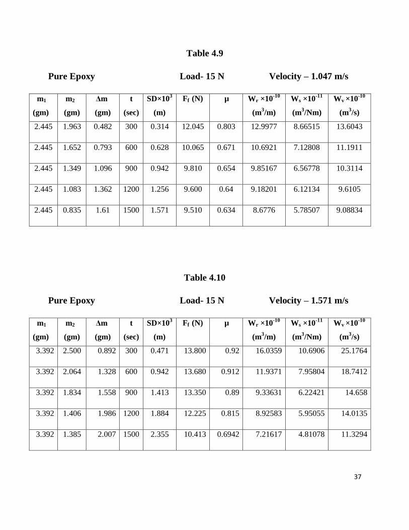
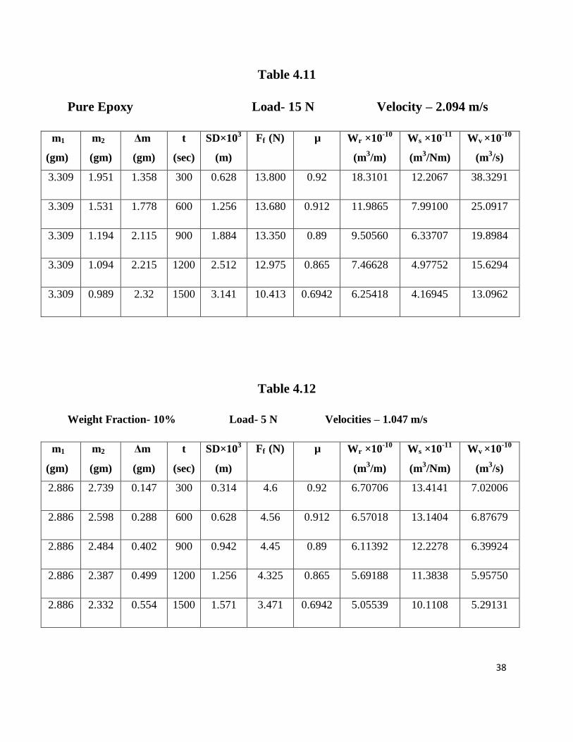
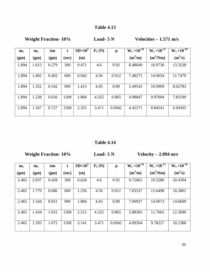
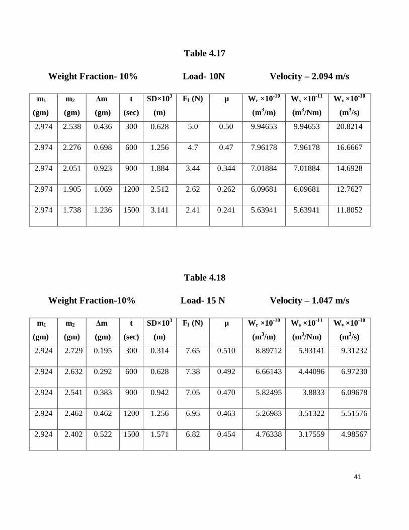
The different values of weight loss, wear rate, volumetric wear rate and specific wear rate under
different test condition is listed in Table-4.3 to 4.37.
Coefficient of friction (µ) can be determined by using following equation:
fF
F ........ (8)
Where, Ff is the frictional force in N obtained from control panel directly and F is the applied
normal force in N.
33
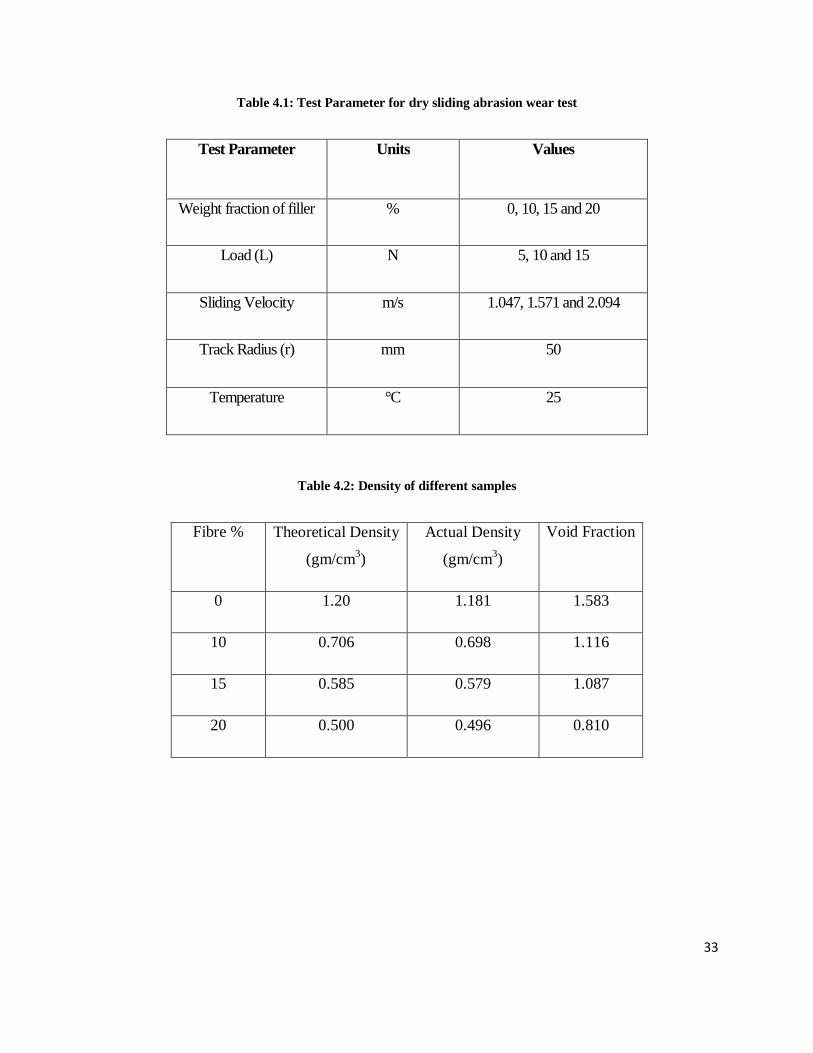
Table 4.1: Test Parameter for dry sliding abrasion wear test
Test Parameter Units Values
Weight fraction of filler % 0, 10, 15 and 20
Load (L) N 5, 10 and 15
Sliding Velocity m/s 1.047, 1.571 and 2.094
Track Radius (r) mm 50
Temperature °C 25
Table 4.2: Density of different samples
Fibre % Theoretical Density
(gm/cm3)
Actual Density
(gm/cm3)
Void Fraction
0 1.20 1.181 1.583
10 0.706 0.698 1.116
15 0.585 0.579 1.087
20 0.500 0.496 0.810
34
Table 4.3
Pure Epoxy Load- 5 N Velocity – 1.047 m/s
m1
(gm)
m2
(gm)
Δm
(gm)
t (sec) SD×103
(m)
Ff (N) µ Wr ×10-10
(m3/m)
Ws ×10-11
(m3/Nm)
Wv ×10-10
(m3/s)
3.389 3.024 0.365 300 0.314 4.61 0.922 9.84268 19.6854 10.302
3.389 2.796 0.593 600 0.628 4.49 0.898 7.99549 15.9910 8.36861
3.389 2.583 0.806 900 0.942 4.35 0.87 7.24493 14.4899 7.58303
3.389 2.489 0.900 1200 1.256 4.17 0.834 6.0674 12.1348 6.35055
3.389 2.368 1.021 1500 1.570 4.01 0.802 5.503 11.006 5.76348
Table 4.4
Pure Epoxy Load- 5 N Velocity – 1.571 m/s
m1
(gm)
m2
(gm)
Δm
(gm)
t
(sec)
SD×103
(m)
Ff (N) µ Wr ×10-10
(m3/m)
Ws ×10-11
(m3/Nm)
Wv ×10-10
(m3/s)
2.618 1.951 0.667 300 0.471 4.6 0.92 11.99001 23.982 18.8259
2.618 1.623 0.995 600 0.942 4.56 0.912 8.9438 17.8876 14.0418
2.618 1.437 1.181 900 1.413 4.45 0.89 7.07714 14.1543 11.1111
2.618 1.407 1.211 1200 1.884 4.325 0.865 5.44269 10.8854 8.54502
2.618 1.397 1.221 1500 2.355 3.971 0.792 4.3901 8.78021 6.89246
35
Table 4.5
Pure Epoxy Load- 5 N Velocity – 2.094 m/s
m1
(gm)
m2
(gm)
Δm
(gm)
t
(sec)
SD×103
(m)
Ff (N) µ Wr ×10-10
(m3/m)
Ws ×10-11
(m3/Nm)
Wv ×10-10
(m3/s)
3.191 2.461 0.73 300 0.628 4.6 0.92 9.84366 19.700 20.60610
3.191 1.997 1.194 600 1.256 4.56 0.912 8.05588 16.100 16.86364
3.191 1.556 1.635 900 1.884 4.45 0.89 7.36827 14.700 15.42424
3.191 1.144 2.047 1200 2.512 4.325 0.865 6.88694 13.800 14.42424
3.191 0.763 2.428 1500 3.140 3.471 0.6942 6.57209 13.100 13.75758
Table 4.6
Pure Epoxy Load- 10 N Velocity – 1.047 m/s
m1
(gm)
m2
(gm)
Δm
(gm)
t
(sec)
SD×103
(m)
Ff (N) µ Wr ×10-10
(m3/m)
Ws ×10-11
(m3/Nm)
Wv ×10-10
(m3/s)
3.182 2.737 0.445 300 0.314 9.2 0.92 12.0000 12.0000 12.5600
3.182 2.435 0.747 600 0.628 9.12 0.912 10.0719 10.0719 10.5419
3.182 2.182 1.000 900 0.942 8.9 0.89 8.98875 8.98875 9.40822
3.182 1.937 1.245 1200 1.256 8.65 0.865 8.39324 8.39324 8.78493
3.182 1.707 1.475 1500 1.570 6.942 0.6942 7.94998 7.94998 8.32628
36
Table 4.7
Pure Epoxy Load- 10 N Velocity – 1.571 m/s
m1
(gm)
m2
(gm)
Δm
(gm)
t
(sec)
SD×103
(m)
Ff (N) µ Wr ×10-10
(m3/m)
Ws ×10-11
(m3/Nm)
Wv ×10-10
(m3/s)
3.625 2.77 0.855 300 0.471 9.2 0.92 15.3708 15.3708 24.1321
3.625 2.448 1.177 600 0.942 9 0.9 10.5798 10.5798 16.6102
3.625 2.208 1.417 900 1.413 8.9 0.89 8.49137 8.49137 13.3315
3.625 2.075 1.55 1200 1.884 8.65 0.865 6.96628 6.96628 10.9371
3.625 1.906 1.719 1500 2.355 6.942 0.6942 6.18066 6.18066 9.70364
Table 4.8
Pure Epoxy Load- 10 N Velocity – 2.094 m/s
m1
(gm)
m2
(gm)
Δm
(gm)
t
(sec)
SD×103
(m)
Ff (N) µ Wr ×10-10
(m3/m)
Ws ×10-11
(m3/Nm)
Wv ×10-10
(m3/s)
2.481 1.243 1.238 300 0.628 9.2 0.92 16.6921 16.6921 34.9421
2.481 0.718 1.763 600 1.256 9.12 0.912 11.8854 11.8854 24.8800
2.481 0.665 1.816 900 1.884 8.9 0.89 8.16178 8.16178 17.0853
2.481 0.582 1.899 1200 2.512 8.65 0.865 6.40111 6.40111 13.3997
2.481 0.483 1.998 1500 3.141 6.942 0.6942 5.38614 5.38614 11.2786
37
Table 4.9
Pure Epoxy Load- 15 N Velocity – 1.047 m/s
m1
(gm)
m2
(gm)
Δm
(gm)
t
(sec)
SD×103
(m)
Ff (N) µ Wr ×10-10
(m3/m)
Ws ×10-11
(m3/Nm)
Wv ×10-10
(m3/s)
2.445 1.963 0.482 300 0.314 12.045 0.803 12.9977 8.66515 13.6043
2.445 1.652 0.793 600 0.628 10.065 0.671 10.6921 7.12808 11.1911
2.445 1.349 1.096 900 0.942 9.810 0.654 9.85167 6.56778 10.3114
2.445 1.083 1.362 1200 1.256 9.600 0.64 9.18201 6.12134 9.6105
2.445 0.835 1.61 1500 1.571 9.510 0.634 8.6776 5.78507 9.08834
Table 4.10
Pure Epoxy Load- 15 N Velocity – 1.571 m/s
m1
(gm)
m2
(gm)
Δm
(gm)
t
(sec)
SD×103
(m)
Ff (N) µ Wr ×10-10
(m3/m)
Ws ×10-11
(m3/Nm)
Wv ×10-10
(m3/s)
3.392 2.500 0.892 300 0.471 13.800 0.92 16.0359 10.6906 25.1764
3.392 2.064 1.328 600 0.942 13.680 0.912 11.9371 7.95804 18.7412
3.392 1.834 1.558 900 1.413 13.350 0.89 9.33631 6.22421 14.658
3.392 1.406 1.986 1200 1.884 12.225 0.815 8.92583 5.95055 14.0135
3.392 1.385 2.007 1500 2.355 10.413 0.6942 7.21617 4.81078 11.3294
38
Table 4.11
Pure Epoxy Load- 15 N Velocity – 2.094 m/s
m1
(gm)
m2
(gm)
Δm
(gm)
t
(sec)
SD×103
(m)
Ff (N) µ Wr ×10-10
(m3/m)
Ws ×10-11
(m3/Nm)
Wv ×10-10
(m3/s)
3.309 1.951 1.358 300 0.628 13.800 0.92 18.3101 12.2067 38.3291
3.309 1.531 1.778 600 1.256 13.680 0.912 11.9865 7.99100 25.0917
3.309 1.194 2.115 900 1.884 13.350 0.89 9.50560 6.33707 19.8984
3.309 1.094 2.215 1200 2.512 12.975 0.865 7.46628 4.97752 15.6294
3.309 0.989 2.32 1500 3.141 10.413 0.6942 6.25418 4.16945 13.0962
Table 4.12
Weight Fraction- 10% Load- 5 N Velocities – 1.047 m/s
m1
(gm)
m2
(gm)
Δm
(gm)
t
(sec)
SD×103
(m)
Ff (N) µ Wr ×10-10
(m3/m)
Ws ×10-11
(m3/Nm)
Wv ×10-10
(m3/s)
2.886 2.739 0.147 300 0.314 4.6 0.92 6.70706 13.4141 7.02006
2.886 2.598 0.288 600 0.628 4.56 0.912 6.57018 13.1404 6.87679
2.886 2.484 0.402 900 0.942 4.45 0.89 6.11392 12.2278 6.39924
2.886 2.387 0.499 1200 1.256 4.325 0.865 5.69188 11.3838 5.95750
2.886 2.332 0.554 1500 1.571 3.471 0.6942 5.05539 10.1108 5.29131
39
Table 4.13
Weight Fraction- 10% Load- 5 N Velocities – 1.571 m/s
m1
(gm)
m2
(gm)
Δm
(gm)
t
(sec)
SD×103
(m)
Ff (N) µ Wr ×10-10
(m3/m)
Ws ×10-11
(m3/Nm)
Wv ×10-10
(m3/s)
1.894 1.615 0.279 300 0.471 4.6 0.92 8.48649 16.9730 13.3238
1.894 1.402 0.492 600 0.942 4.56 0.912 7.48271 14.9654 11.7479
1.894 1.352 0.542 900 1.413 4.45 0.89 5.49543 10.9909 8.62783
1.894 1.238 0.656 1200 1.884 4.325 0.865 4.98847 9.97694 7.83190
1.894 1.167 0.727 1500 2.355 3.471 0.6942 4.42271 8.84541 6.94365
Table 4.14
Weight Fraction- 10% Load- 5 N Velocity – 2.094 m/s
m1
(gm)
m2
(gm)
Δm
(gm)
t
(sec)
SD×103
(m)
Ff (N) µ Wr ×10-10
(m3/m)
Ws ×10-11
(m3/Nm)
Wv ×10-10
(m3/s)
2.465 2.037 0.428 300 0.628 4.6 0.92 9.75961 19.5280 20.4394
2.465 1.779 0.686 600 1.256 4.56 0.912 7.83337 15.6498 16.3801
2.465 1.544 0.921 900 1.884 4.45 0.89 7.00937 14.0073 14.6609
2.465 1.434 1.031 1200 2.512 4.325 0.865 5.88305 11.7602 12.3090
2.465 1.393 1.072 1500 3.141 3.471 0.6942 4.89264 9.78227 10.2388

40
Table 4.15
Weight Fraction- 10% Load- 10 N Velocity – 1.047 m/s
m1
(gm)
m2
(gm)
Δm
(gm)
t
(sec)
SD×103
(m)
Ff (N) µ Wr ×10-10
(m3/m)
Ws ×10-11
(m3/Nm)
Wv ×10-10
(m3/s)
2.604 2.375 0.229 300 0.314 5.7 0.57 10.5849 10.58490 10.9360
2.604 2.304 0.3 600 0.628 5.47 0.547 6.93334 6.93334 7.16332
2.604 2.253 0.351 900 0.942 4.9 0.49 5.40800 5.40800 5.58739
2.604 2.207 0.397 1200 1.256 4.34 0.434 4.58756 4.58756 4.73973
2.604 2.177 0.427 1500 1.571 4.015 0.4015 3.94738 3.94738 4.07832
Table 4.16
Weight Fraction- 10% Load- 10 N Velocity – 1.571 m/s
m1
(gm)
m2
(gm)
Δm
(gm)
t
(sec)
SD×103
(m)
Ff (N) µ Wr ×10-10
(m3/m)
Ws ×10-11
(m3/Nm)
Wv ×10-10
(m3/s)
2.104 1.72 0.384 300 0.471 4.733 0.4733 11.6803 11.6803 18.3381
2.104 1.525 0.579 600 0.942 3.557 0.3557 8.80587 8.80587 13.8252
2.104 1.469 0.635 900 1.413 3.501 0.3501 6.43837 6.43837 10.1082
2.104 1.431 0.673 1200 1.884 3.4 0.34 5.11775 5.11775 8.03486
2.104 1.319 0.785 1500 2.355 3.0 0.3 4.77555 4.77555 7.49761
41
Table 4.17
Weight Fraction- 10% Load- 10N Velocity – 2.094 m/s
m1
(gm)
m2
(gm)
Δm
(gm)
t
(sec)
SD×103
(m)
Ff (N) µ Wr ×10-10
(m3/m)
Ws ×10-11
(m3/Nm)
Wv ×10-10
(m3/s)
2.974 2.538 0.436 300 0.628 5.0 0.50 9.94653 9.94653 20.8214
2.974 2.276 0.698 600 1.256 4.7 0.47 7.96178 7.96178 16.6667
2.974 2.051 0.923 900 1.884 3.44 0.344 7.01884 7.01884 14.6928
2.974 1.905 1.069 1200 2.512 2.62 0.262 6.09681 6.09681 12.7627
2.974 1.738 1.236 1500 3.141 2.41 0.241 5.63941 5.63941 11.8052
Table 4.18
Weight Fraction-10% Load- 15 N Velocity – 1.047 m/s
m1
(gm)
m2
(gm)
Δm
(gm)
t
(sec)
SD×103
(m)
Ff (N) µ Wr ×10-10
(m3/m)
Ws ×10-11
(m3/Nm)
Wv ×10-10
(m3/s)
2.924 2.729 0.195 300 0.314 7.65 0.510 8.89712 5.93141 9.31232
2.924 2.632 0.292 600 0.628 7.38 0.492 6.66143 4.44096 6.97230
2.924 2.541 0.383 900 0.942 7.05 0.470 5.82495 3.8833 6.09678
2.924 2.462 0.462 1200 1.256 6.95 0.463 5.26983 3.51322 5.51576
2.924 2.402 0.522 1500 1.571 6.82 0.454 4.76338 3.17559 4.98567
42
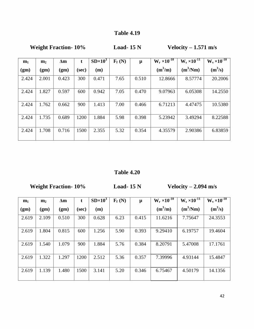
Table 4.19
Weight Fraction- 10% Load- 15 N Velocity – 1.571 m/s
m1
(gm)
m2
(gm)
Δm
(gm)
t
(sec)
SD×103
(m)
Ff (N) µ Wr ×10-10
(m3/m)
Ws ×10-11
(m3/Nm)
Wv ×10-10
(m3/s)
2.424 2.001 0.423 300 0.471 7.65 0.510 12.8666 8.57774 20.2006
2.424 1.827 0.597 600 0.942 7.05 0.470 9.07963 6.05308 14.2550
2.424 1.762 0.662 900 1.413 7.00 0.466 6.71213 4.47475 10.5380
2.424 1.735 0.689 1200 1.884 5.98 0.398 5.23942 3.49294 8.22588
2.424 1.708 0.716 1500 2.355 5.32 0.354 4.35579 2.90386 6.83859
Table 4.20
Weight Fraction- 10% Load- 15 N Velocity – 2.094 m/s
m1
(gm)
m2
(gm)
Δm
(gm)
t
(sec)
SD×103
(m)
Ff (N) µ Wr ×10-10
(m3/m)
Ws ×10-11
(m3/Nm)
Wv ×10-10
(m3/s)
2.619 2.109 0.510 300 0.628 6.23 0.415 11.6216 7.75647 24.3553
2.619 1.804 0.815 600 1.256 5.90 0.393 9.29410 6.19757 19.4604
2.619 1.540 1.079 900 1.884 5.76 0.384 8.20791 5.47008 17.1761
2.619 1.322 1.297 1200 2.512 5.36 0.357 7.39996 4.93144 15.4847
2.619 1.139 1.480 1500 3.141 5.20 0.346 6.75467 4.50179 14.1356

43
Table 4.21
Weight Fraction- 15% Load- 5 N Velocity – 1.047 m/s
m1
(gm)
m2
(gm)
Δm
(gm)
t
(sec)
SD×103
(m)
Ff (N) µ Wr ×10-10
(m3/m)
Ws ×10-11
(m3/Nm)
Wv ×10-10
(m3/s)
2.989 2.889 0.100 300 0.314 4.38 0.876 5.50037 11.0007 5.75705
2.989 2.819 0.170 600 0.628 4.26 0.852 4.67531 9.35063 4.89349
2.989 2.762 0.227 900 0.942 4.22 0.844 4.16195 8.32389 4.35617
2.989 2.703 0.286 1200 1.256 4.16 0.832 3.93276 7.86553 4.11629
2.989 2.65 0.339 1500 1.571 3.471 0.6942 3.72925 7.4585 3.90328
Table 4.22
Weight Fraction- 15% Load- 5 N Velocity – 1.571 m/s
m1
(gm)
m2
(gm)
Δm
(gm)
t
(sec)
SD×103
(m)
Ff (N) µ Wr ×10-10
(m3/m)
Ws ×10-11
(m3/Nm)
Wv ×10-10
(m3/s)
2.659 2.502 0.157 300 0.471 4.42 0.884 5.75705 11.5141 9.03857
2.659 2.378 0.281 600 0.942 4.11 0.822 5.15201 10.3040 8.08866
2.659 2.287 0.372 900 1.413 3.86 0.772 4.54697 9.09394 7.13874
2.659 2.250 0.409 1200 1.884 3.71 0.742 3.74942 7.49884 5.88659
2.659 2.233 0.426 1500 2.355 3.69 0.738 3.12421 6.24842 4.90501
44
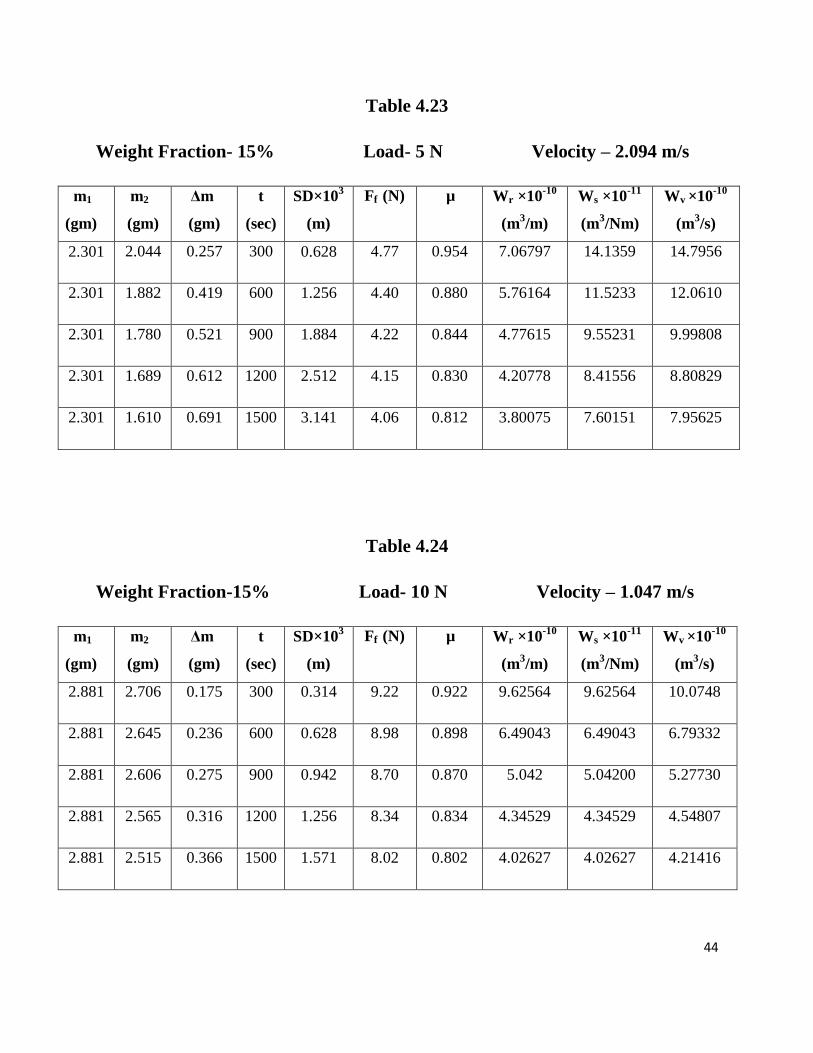
Table 4.23
Weight Fraction- 15% Load- 5 N Velocity – 2.094 m/s
m1
(gm)
m2
(gm)
Δm
(gm)
t
(sec)
SD×103
(m)
Ff (N) µ Wr ×10-10
(m3/m)
Ws ×10-11
(m3/Nm)
Wv ×10-10
(m3/s)
2.301 2.044 0.257 300 0.628 4.77 0.954 7.06797 14.1359 14.7956
2.301 1.882 0.419 600 1.256 4.40 0.880 5.76164 11.5233 12.0610
2.301 1.780 0.521 900 1.884 4.22 0.844 4.77615 9.55231 9.99808
2.301 1.689 0.612 1200 2.512 4.15 0.830 4.20778 8.41556 8.80829
2.301 1.610 0.691 1500 3.141 4.06 0.812 3.80075 7.60151 7.95625
Table 4.24
Weight Fraction-15% Load- 10 N Velocity – 1.047 m/s
m1
(gm)
m2
(gm)
Δm
(gm)
t
(sec)
SD×103
(m)
Ff (N) µ Wr ×10-10
(m3/m)
Ws ×10-11
(m3/Nm)
Wv ×10-10
(m3/s)
2.881 2.706 0.175 300 0.314 9.22 0.922 9.62564 9.62564 10.0748
2.881 2.645 0.236 600 0.628 8.98 0.898 6.49043 6.49043 6.79332
2.881 2.606 0.275 900 0.942 8.70 0.870 5.042 5.04200 5.27730
2.881 2.565 0.316 1200 1.256 8.34 0.834 4.34529 4.34529 4.54807
2.881 2.515 0.366 1500 1.571 8.02 0.802 4.02627 4.02627 4.21416
45
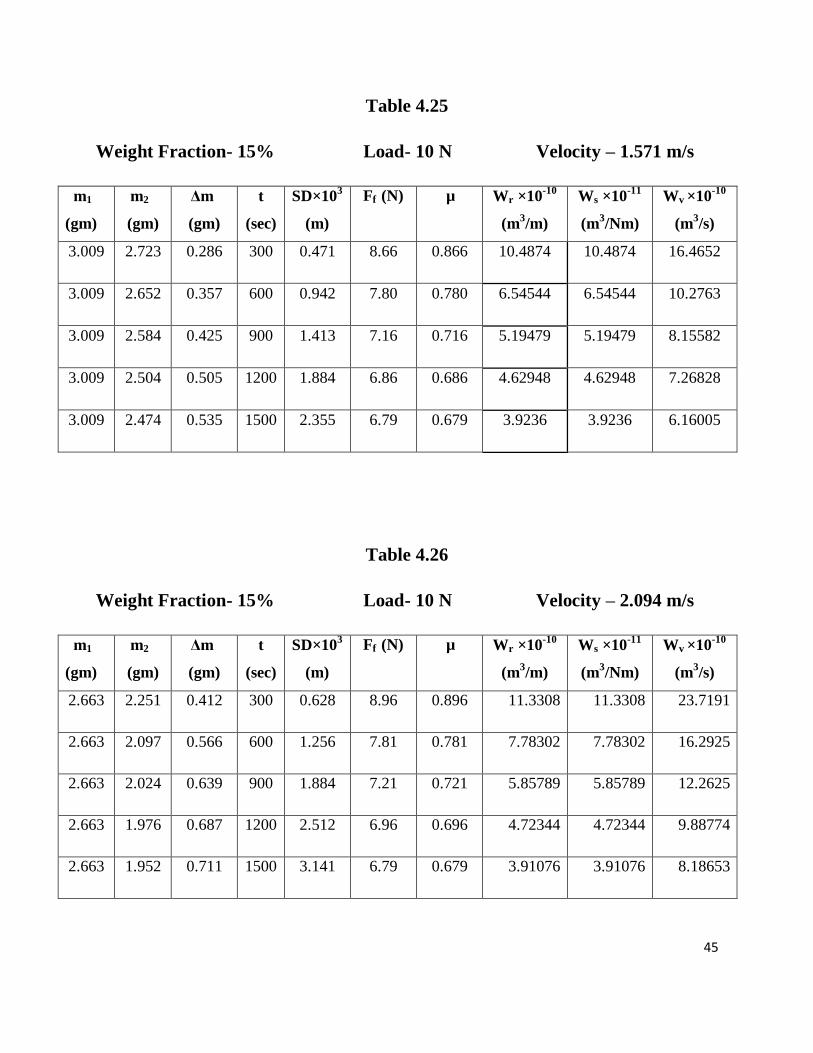
Table 4.25
Weight Fraction- 15% Load- 10 N Velocity – 1.571 m/s
m1
(gm)
m2
(gm)
Δm
(gm)
t
(sec)
SD×103
(m)
Ff (N) µ Wr ×10-10
(m3/m)
Ws ×10-11
(m3/Nm)
Wv ×10-10
(m3/s)
3.009 2.723 0.286 300 0.471 8.66 0.866 10.4874 10.4874 16.4652
3.009 2.652 0.357 600 0.942 7.80 0.780 6.54544 6.54544 10.2763
3.009 2.584 0.425 900 1.413 7.16 0.716 5.19479 5.19479 8.15582
3.009 2.504 0.505 1200 1.884 6.86 0.686 4.62948 4.62948 7.26828
3.009 2.474 0.535 1500 2.355 6.79 0.679 3.9236 3.9236 6.16005
Table 4.26
Weight Fraction- 15% Load- 10 N Velocity – 2.094 m/s
m1
(gm)
m2
(gm)
Δm
(gm)
t
(sec)
SD×103
(m)
Ff (N) µ Wr ×10-10
(m3/m)
Ws ×10-11
(m3/Nm)
Wv ×10-10
(m3/s)
2.663 2.251 0.412 300 0.628 8.96 0.896 11.3308 11.3308 23.7191
2.663 2.097 0.566 600 1.256 7.81 0.781 7.78302 7.78302 16.2925
2.663 2.024 0.639 900 1.884 7.21 0.721 5.85789 5.85789 12.2625
2.663 1.976 0.687 1200 2.512 6.96 0.696 4.72344 4.72344 9.88774
2.663 1.952 0.711 1500 3.141 6.79 0.679 3.91076 3.91076 8.18653

46
Table 4.27
Weight Fraction- 15% Load- 15 N Velocity – 1.047m/s
m1
(gm)
m2
(gm)
Δm
(gm)
t
(sec)
SD×103
(m)
Ff (N) µ Wr ×10-10
(m3/m)
Ws ×10-11
(m3/Nm)
Wv ×10-10
(m3/s)
2.351 2.165 0.186 300 0.314 12.05 0.803 10.2307 6.82046 10.7081
2.351 2.115 0.236 600 0.628 10.07 0.671 6.49043 4.32696 6.79332
2.351 2.083 0.268 900 0.942 9.82 0.654 4.91366 3.27578 5.14297
2.351 2.037 0.314 1200 1.256 9.60 0.640 4.31779 2.87853 4.51929
2.351 2.001 0.35 1500 1.571 9.52 0.634 3.84781 2.5652 4.02994
Table 4.28
Weight Fraction- 15% Load- 15 N Velocity – 1.571 m/s
m1
(gm)
m2
(gm)
Δm
(gm)
t
(sec)
SD×103
(m)
Ff (N) µ Wr ×10-10
(m3/m)
Ws ×10-11
(m3/Nm)
Wv ×10-10
(m3/s)
2.847 2.529 0.318 300 0.471 12.95 0.863 11.6608 7.77385 18.3074
2.847 2.472 0.375 600 0.942 12.25 0.816 6.87546 4.58364 10.7945
2.847 2.461 0.386 900 1.413 11.67 0.778 4.71809 3.1454 7.40741
2.847 2.356 0.491 1200 1.884 10.95 0.730 4.50113 3.00076 7.06678
2.847 2.326 0.521 1500 2.355 10.51 0.700 3.82092 2.54728 5.99885
47
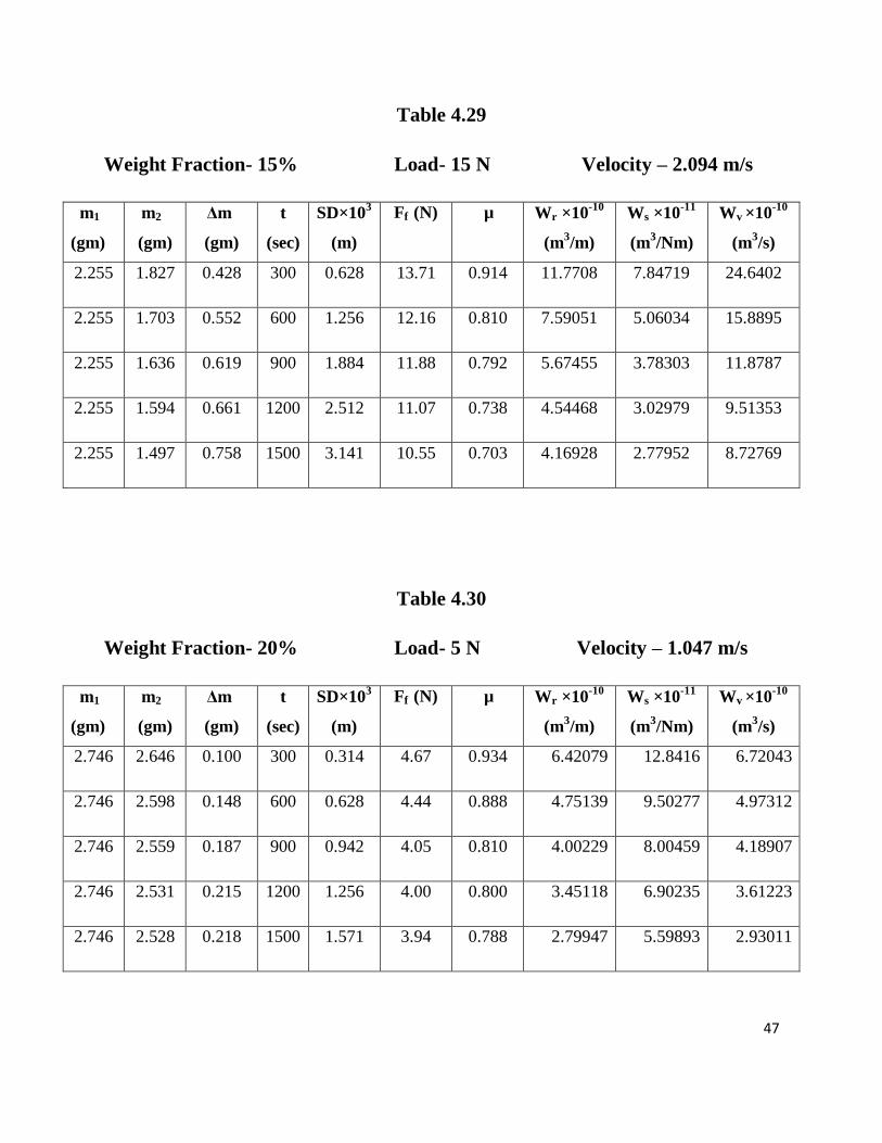
Table 4.29
Weight Fraction- 15% Load- 15 N Velocity – 2.094 m/s
m1
(gm)
m2
(gm)
Δm
(gm)
t
(sec)
SD×103
(m)
Ff (N) µ Wr ×10-10
(m3/m)
Ws ×10-11
(m3/Nm)
Wv ×10-10
(m3/s)
2.255 1.827 0.428 300 0.628 13.71 0.914 11.7708 7.84719 24.6402
2.255 1.703 0.552 600 1.256 12.16 0.810 7.59051 5.06034 15.8895
2.255 1.636 0.619 900 1.884 11.88 0.792 5.67455 3.78303 11.8787
2.255 1.594 0.661 1200 2.512 11.07 0.738 4.54468 3.02979 9.51353
2.255 1.497 0.758 1500 3.141 10.55 0.703 4.16928 2.77952 8.72769
Table 4.30
Weight Fraction- 20% Load- 5 N Velocity – 1.047 m/s
m1
(gm)
m2
(gm)
Δm
(gm)
t
(sec)
SD×103
(m)
Ff (N) µ Wr ×10-10
(m3/m)
Ws ×10-11
(m3/Nm)
Wv ×10-10
(m3/s)
2.746 2.646 0.100 300 0.314 4.67 0.934 6.42079 12.8416 6.72043
2.746 2.598 0.148 600 0.628 4.44 0.888 4.75139 9.50277 4.97312
2.746 2.559 0.187 900 0.942 4.05 0.810 4.00229 8.00459 4.18907
2.746 2.531 0.215 1200 1.256 4.00 0.800 3.45118 6.90235 3.61223
2.746 2.528 0.218 1500 1.571 3.94 0.788 2.79947 5.59893 2.93011
48
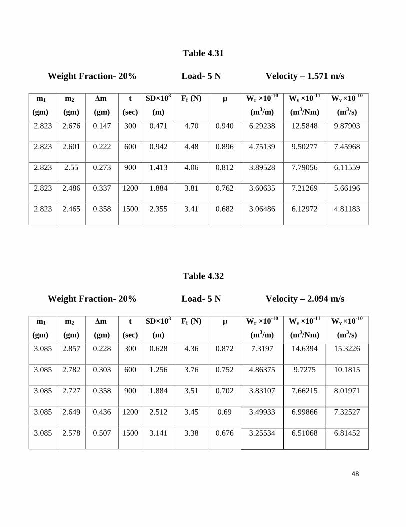
Table 4.31
Weight Fraction- 20% Load- 5 N Velocity – 1.571 m/s
m1
(gm)
m2
(gm)
Δm
(gm)
t
(sec)
SD×103
(m)
Ff (N) µ Wr ×10-10
(m3/m)
Ws ×10-11
(m3/Nm)
Wv ×10-10
(m3/s)
2.823 2.676 0.147 300 0.471 4.70 0.940 6.29238 12.5848 9.87903
2.823 2.601 0.222 600 0.942 4.48 0.896 4.75139 9.50277 7.45968
2.823 2.55 0.273 900 1.413 4.06 0.812 3.89528 7.79056 6.11559
2.823 2.486 0.337 1200 1.884 3.81 0.762 3.60635 7.21269 5.66196
2.823 2.465 0.358 1500 2.355 3.41 0.682 3.06486 6.12972 4.81183
Table 4.32
Weight Fraction- 20% Load- 5 N Velocity – 2.094 m/s
m1
(gm)
m2
(gm)
Δm
(gm)
t
(sec)
SD×103
(m)
Ff (N) µ Wr ×10-10
(m3/m)
Ws ×10-11
(m3/Nm)
Wv ×10-10
(m3/s)
3.085 2.857 0.228 300 0.628 4.36 0.872 7.3197 14.6394 15.3226
3.085 2.782 0.303 600 1.256 3.76 0.752 4.86375 9.7275 10.1815
3.085 2.727 0.358 900 1.884 3.51 0.702 3.83107 7.66215 8.01971
3.085 2.649 0.436 1200 2.512 3.45 0.69 3.49933 6.99866 7.32527
3.085 2.578 0.507 1500 3.141 3.38 0.676 3.25534 6.51068 6.81452
49
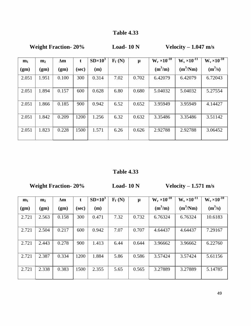
Table 4.33
Weight Fraction- 20% Load- 10 N Velocity – 1.047 m/s
m1
(gm)
m2
(gm)
Δm
(gm)
t
(sec)
SD×103
(m)
Ff (N) µ Wr ×10-10
(m3/m)
Ws ×10-11
(m3/Nm)
Wv ×10-10
(m3/s)
2.051 1.951 0.100 300 0.314 7.02 0.702 6.42079 6.42079 6.72043
2.051 1.894 0.157 600 0.628 6.80 0.680 5.04032 5.04032 5.27554
2.051 1.866 0.185 900 0.942 6.52 0.652 3.95949 3.95949 4.14427
2.051 1.842 0.209 1200 1.256 6.32 0.632 3.35486 3.35486 3.51142
2.051 1.823 0.228 1500 1.571 6.26 0.626 2.92788 2.92788 3.06452
Table 4.33
Weight Fraction- 20% Load- 10 N Velocity – 1.571 m/s
m1
(gm)
m2
(gm)
Δm
(gm)
t
(sec)
SD×103
(m)
Ff (N) µ Wr ×10-10
(m3/m)
Ws ×10-11
(m3/Nm)
Wv ×10-10
(m3/s)
2.721 2.563 0.158 300 0.471 7.32 0.732 6.76324 6.76324 10.6183
2.721 2.504 0.217 600 0.942 7.07 0.707 4.64437 4.64437 7.29167
2.721 2.443 0.278 900 1.413 6.44 0.644 3.96662 3.96662 6.22760
2.721 2.387 0.334 1200 1.884 5.86 0.586 3.57424 3.57424 5.61156
2.721 2.338 0.383 1500 2.355 5.65 0.565 3.27889 3.27889 5.14785

50
Table 4.34
Weight Fraction- 20% Load- 10 N Velocity – 2.094 m/s
m1
(gm)
m2
(gm)
Δm
(gm)
t
(sec)
SD×103
(m)
Ff (N) µ Wr ×10-10
(m3/m)
Ws ×10-11
(m3/Nm)
Wv ×10-10
(m3/s)
2.568 2.321 0.247 300 0.628 7.80 0.780 7.92968 7.92968 16.5995
2.568 2.272 0.296 600 1.256 6.47 0.647 4.75139 4.75139 9.94624
2.568 2.171 0.397 900 1.884 5.60 0.560 4.24842 4.24842 8.89337
2.568 2.114 0.454 1200 2.512 4.77 0.477 3.6438 3.6438 7.62769
2.568 2.051 0.517 1500 3.141 4.23 0.423 3.31955 3.31955 6.94892
Table 4.35
Weight Fraction-20% Load- 15 N Velocity – 1.047 m/s
m1
(gm)
m2
(gm)
Δm
(gm)
t
(sec)
SD×103
(m)
Ff (N) µ Wr ×10-10
(m3/m)
Ws ×10-11
(m3/Nm)
Wv ×10-10
(m3/s)
2.725 2.620 0.105 300 0.314 12.77 0.851 6.74183 4.49456 7.05645
2.725 2.556 0.169 600 0.628 11.81 0.787 5.42557 3.61705 5.67876
2.725 2.498 0.227 900 0.942 11.14 0.742 4.85840 3.23893 5.08513
2.725 2.470 0.255 1200 1.256 10.78 0.718 4.09326 2.72884 4.28427
2.725 2.438 0.287 1500 1.571 10.52 0.701 3.68319 2.45546 3.85753
51
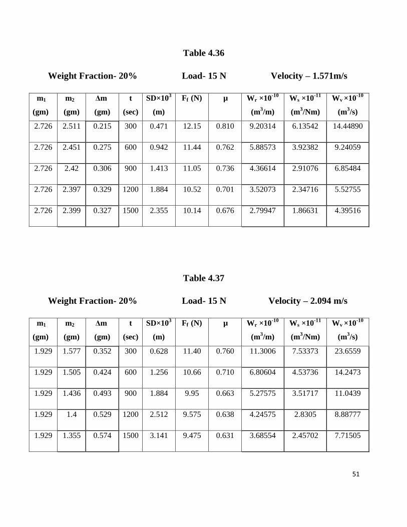
Table 4.36
Weight Fraction- 20% Load- 15 N Velocity – 1.571m/s
m1
(gm)
m2
(gm)
Δm
(gm)
t
(sec)
SD×103
(m)
Ff (N) µ Wr ×10-10
(m3/m)
Ws ×10-11
(m3/Nm)
Wv ×10-10
(m3/s)
2.726 2.511 0.215 300 0.471 12.15 0.810 9.20314 6.13542 14.44890
2.726 2.451 0.275 600 0.942 11.44 0.762 5.88573 3.92382 9.24059
2.726 2.42 0.306 900 1.413 11.05 0.736 4.36614 2.91076 6.85484
2.726 2.397 0.329 1200 1.884 10.52 0.701 3.52073 2.34716 5.52755
2.726 2.399 0.327 1500 2.355 10.14 0.676 2.79947 1.86631 4.39516
Table 4.37
Weight Fraction- 20% Load- 15 N Velocity – 2.094 m/s
m1
(gm)
m2
(gm)
Δm
(gm)
t
(sec)
SD×103
(m)
Ff (N) µ Wr ×10-10
(m3/m)
Ws ×10-11
(m3/Nm)
Wv ×10-10
(m3/s)
1.929 1.577 0.352 300 0.628 11.40 0.760 11.3006 7.53373 23.6559
1.929 1.505 0.424 600 1.256 10.66 0.710 6.80604 4.53736 14.2473
1.929 1.436 0.493 900 1.884 9.95 0.663 5.27575 3.51717 11.0439
1.929 1.4 0.529 1200 2.512 9.575 0.638 4.24575 2.8305 8.88777
1.929 1.355 0.574 1500 3.141 9.475 0.631 3.68554 2.45702 7.71505

52
Fig.4.6: Variation of abrasive wear rate with sliding distance at 5N load and 200 rpm
Fig.4.7: Variation of abrasive wear rate with sliding distance at 10 N load and 200 rpm
53
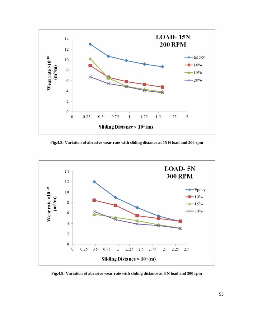
Fig.4.8: Variation of abrasive wear rate with sliding distance at 15 N load and 200 rpm
Fig.4.9: Variation of abrasive wear rate with sliding distance at 5 N load and 300 rpm
54
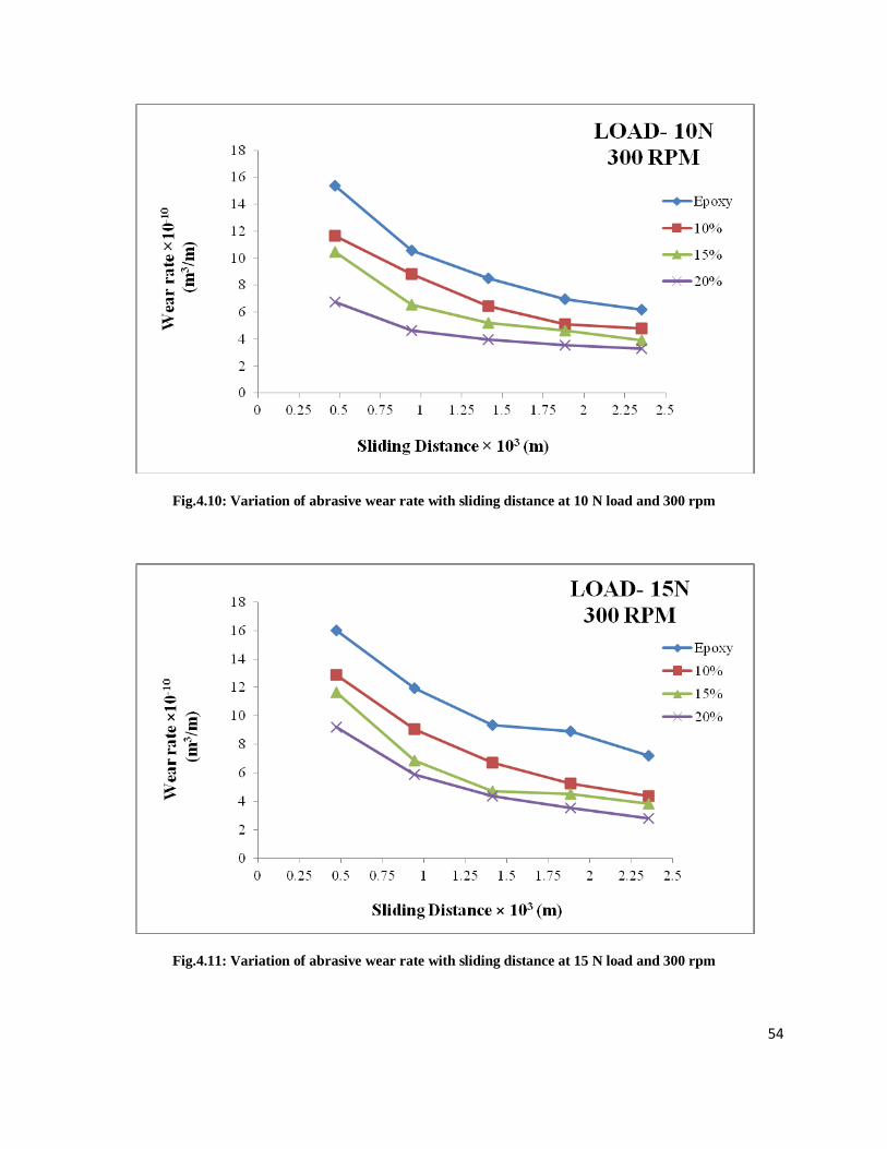
Fig.4.10: Variation of abrasive wear rate with sliding distance at 10 N load and 300 rpm
Fig.4.11: Variation of abrasive wear rate with sliding distance at 15 N load and 300 rpm

55
Fig.4.12: Variation of abrasive wear rate with sliding distance at 5 N load and 400 rpm
Fig.4.13: Variation of abrasive wear rate with sliding distance at 10 N load and 400 rpm
56
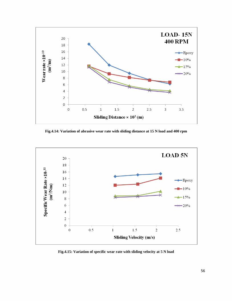
Fig.4.14: Variation of abrasive wear rate with sliding distance at 15 N load and 400 rpm
Fig.4.15: Variation of specific wear rate with sliding velocity at 5 N load
57
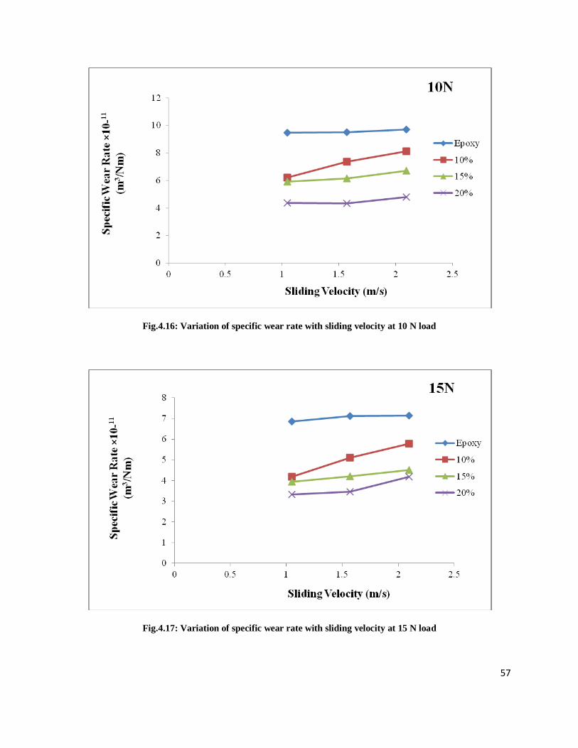
Fig.4.16: Variation of specific wear rate with sliding velocity at 10 N load
Fig.4.17: Variation of specific wear rate with sliding velocity at 15 N load
58
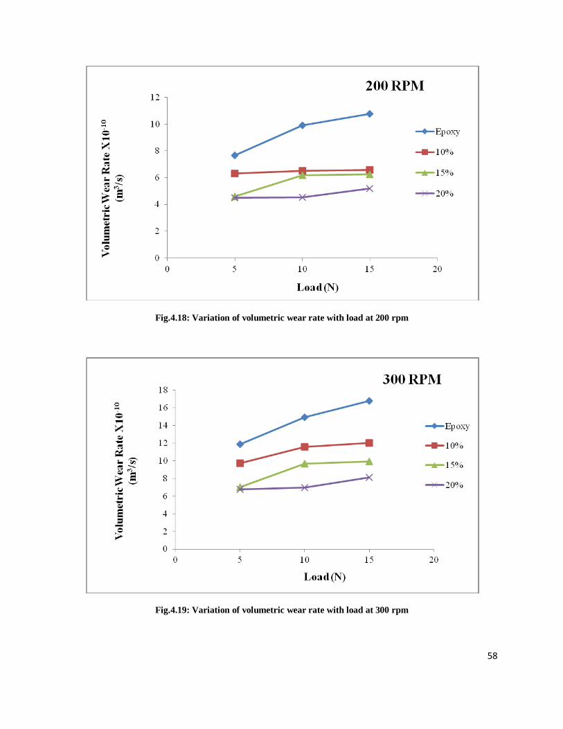
Fig.4.18: Variation of volumetric wear rate with load at 200 rpm
Fig.4.19: Variation of volumetric wear rate with load at 300 rpm
59
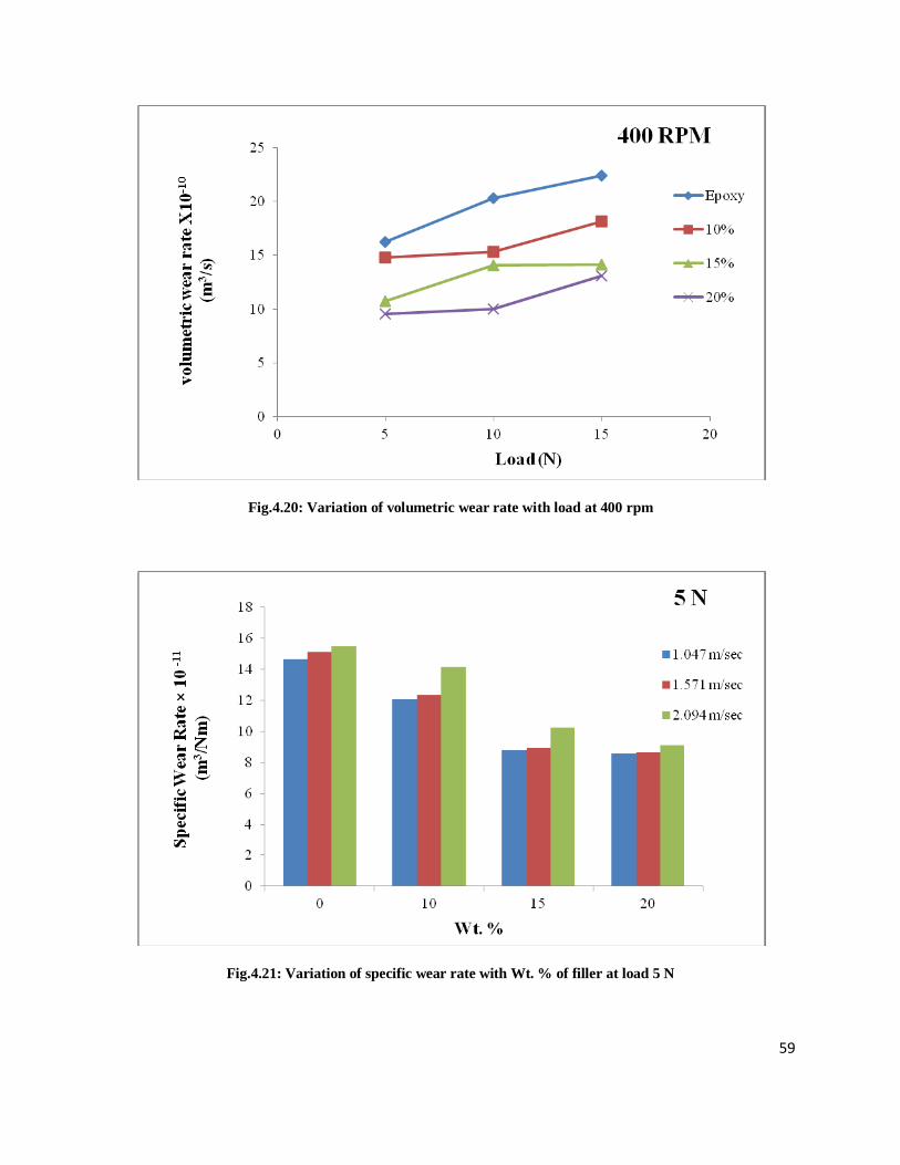
Fig.4.20: Variation of volumetric wear rate with load at 400 rpm
Fig.4.21: Variation of specific wear rate with Wt. % of filler at load 5 N
60
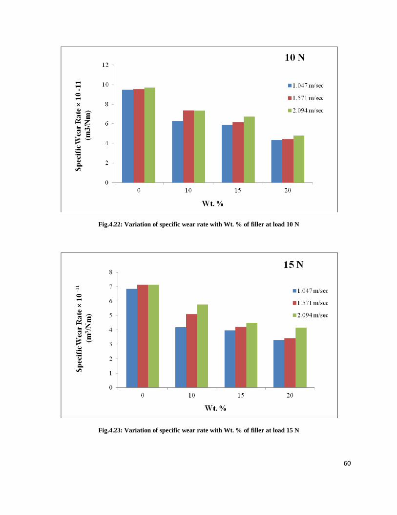
Fig.4.22: Variation of specific wear rate with Wt. % of filler at load 10 N
Fig.4.23: Variation of specific wear rate with Wt. % of filler at load 15 N
61
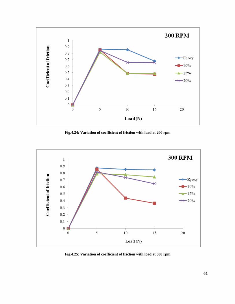
Fig.4.24: Variation of coefficient of friction with load at 200 rpm
Fig.4.25: Variation of coefficient of friction with load at 300 rpm
62
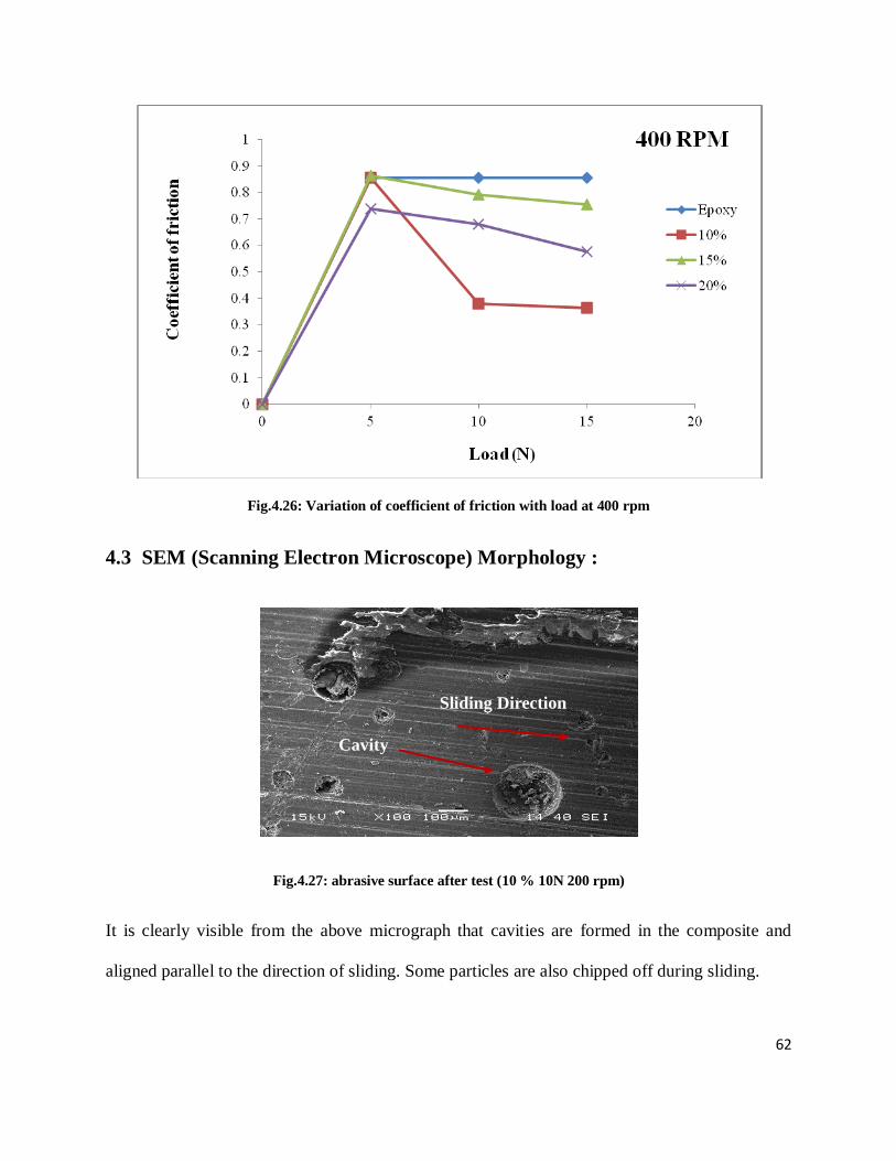
Fig.4.26: Variation of coefficient of friction with load at 400 rpm
4.3 SEM (Scanning Electron Microscope) Morphology :
Fig.4.27: abrasive surface after test (10 % 10N 200 rpm)
It is clearly visible from the above micrograph that cavities are formed in the composite and
aligned parallel to the direction of sliding. Some particles are also chipped off during sliding.
Sliding Direction
Cavity

63
(a) (b)
Fig.4.28 (a) and (b): abrasive surface after test (20 % 10N 300 rpm)
In the above micrograpg cavities are formed with larger depth. Fig. 4.28(b) shows the depth of
cavities at higher magnification. This might have happened due to the abrasive particles
penetration and subsequent removal from the matrix at higher velocity.
(a) (b)
Fig.4.29 (a) and (b): abrasive surface after test (20 % 10N 400 rpm)
High Depth Cavity
Cavity in rolling direction
Chipping off HGM

64
In figure 4.29 (a) depth of cavities are less. Cavities are formed along the rolling direction.
Chipping up of HGM particles are visible at some places but groove formation depth is less
hence we get higher wear resistance. This might happened because at higher velocity (400 rpm)
the abrasive particles are getting less time for penetration at a particular place. So that they did
not formed deeper groove at removal particles from that location. Fig.4.29 (b) shows the same
micrograph at higher magnification.
4.4 RESULTS AND DISCUSSION :
On the basis of experimental and tabulated (4.3 to 4.37) result several graphs are plotted and
presented in fig. 4.6 to 4.26 for different weight fraction of hollow glass microsphere (HGM) as
reinforcement under different test condition.
Figs. 4.6 to 4.14 exhibits the variation of dry sliding abrasive wear rate with increase in sliding
distance for different rpm (200, 300 and 400) at different loads (5, 10 and 15 N). It is clear from
the plots that with addition of hollow glass microsphere particulate the abrasive wear resistance
of epoxy matrix increases. At longer sliding distance there is less exclusion of material because
of low penetration of abrasive particles into the composite specimen. At 20 wt. % HGM abrasive
wear rate is minimum at all testing conditions.
Fig. 4.15 to 4.17 shows the variation of specific wear rate of different wt. % (0, 10, 15 and 20) of
filler composites with sliding velocity at different loads (5N, 10N and 15 N). From the plot it is
clear that the specific wear rate increases as the sliding velocity increase from 1.0471 m/sec to
2.094 m/sec. This might happened due to generation of frictional heat at the interface.
65
S. Basavarajappa et al. [25] also examined the same behaviour of epoxy and glass composite
filled with graphite and silicon carbide particulates.
The deviation of volumetric wear rate with normal applied loads for different wt. % of
particulate filled composites at different sliding velocities is represented in figs. 4.18 to 4.20.
Volumetric wear rate is increases with increase of normal applied loads. At low value of normal
load i.e. 5 N the wear rate was comparatively low due to low diffusion and less number of
abrasive particles in action with rubbing surfaces. At greater value of load large number of rough
particles comes into action and produces large number of grooves due to which wear rate
increases. C. Kanchanomai et al. [38] also observed the increase in volumetric wear loss with
increase in normal applied load at all sliding speeds. Cirino et al. [39] examined the similar effect
in case of carbon epoxy composite and Verma et al. [40] also examined the similar effect in case
of GRP composite.
It is clear from the figs. 4.21 to 4.23 that with increase in wt. % (0, 10, 15 and 20) of HGM of
filler the specific wear rate decrease and it is lowest for 20 wt. % filler.
Fig. 4.24 to 4.26 represents the variation of coefficient of friction with normal applied loads. It is
clear from plot that at initial stage the value of friction coefficient is high but as the value of load
is increase the value of friction coefficient decreases and finally it become steady. S.R. Chauhan
et al. [41] also examined the same frictional behaviour for composite made by reinforcement of
silicon carbide filled glass fibre and glass fibre in vinylester under water and dry lubricated
sliding environment.

CHAPTER 5
CONCLUSION AND FUTURE SCOPE
66
Chapter 5
__________________________________________________________
5.1 CONCLUSION
Following conclusion can be drawn from the experimental investigation:
1. Density of composite was low as compared to neat epoxy so it can be consider as an
applicable light material. With increase in filler content the density of composite will
decrease.
2. On increasing the filler content the impact and tensile strength of composite increases.
Best mechanical properties were obtained at the filler content of 20 weight fraction.
3. The inclusion of hollow glass microsphere into epoxy can considerably increase abrasive
wear resistance of composite. At filler content of 20 weight fraction better wear
resistance properties were obtained.
4. On increasing sliding distance abrasive wear rate continuously decreases and reach upto a
steady state in multi-pass situations.
5. Specific wear rate increase with increase in sliding velocity. Irrespective of load it is
minimum for filler content of 20 weight fraction.
6. Coefficient of friction at initial stage it increases to a higher value but after some time it
decreases and reached a steady state value.
67
5.2 SCOPE FOR FUTURE RESEARCH
1. The current research can be further extended to filler content beyond 20 weight fractions.
2. By surface modification bonding strength between filler and matrix can be increase so
that better mechanical properties can be achieved.
3. Apart from hand lay-up and compression moulding technique other technique can be
used for fabrication.
4. The current experimental work on composite has given better wear resistance for dry
sliding wear test. This can further be extended to other tribological tests like erosion, dry
sand abrasion test etc to make a final conclusion on the suitability of the developed
composite for different applications.

REFERENCES:

68
References
__________________________________________________________
[1]. Hutchings, I.M. (1992), Tribology: friction and wear of engineering materials. CRC Press.
[2]. Kranthi, G. & Satapathy, A. (2010), Evaluation and prediction of wear response of pine
wood dust filled epoxy composites using neural computation. Computational Materials
Science, 49, 609–614.
[3]. Gregory, S.W., Freudenberg, K.D., Bhimaraj, P. & Schadler, L.S. (2003), A study on the
friction and wear behavior of PTFE filled with alumina nanoparticles. Wear, 254 (5-6),
573–580.
[4]. Rothon, R.N. (1999), Mineral fillers in thermoplastics: filler characterization and manufac-
ture Advances in Polymer Science, 139, pp 67–107.
[5]. Suresha, B., Rajesh, B.N., Subbaya, K.M., Ravi Kumar, B.N. & Chandramohan, G. (2010),
Influence of graphite filler on two-body abrasive wear behavior of carbon fabric reinforced
epoxy composites. Materials and Design, 31, pp 1833–1841.
[6]. Mohan, N., Natarajan, S. & KumareshBabu, S.P. (2011), Abrasive wear behaviour of hard
powders filled glass fabric epoxy hybrid composites. Materials and Design, 32, pp
1704–1709.
[7]. Schwartz, C.J. & Bahadur, S. (2001), The role of filler deformability, filler–polymer
bending, and counterface material on the tribological behaviour of polyphenylene
sulfide.Wear, 251, pp 1532–1540.
[8]. Nayak, R., Dora, P.T. & Satapathy, A. (2010), A computational and experimental
investigation on thermal conductivity of particle reinforced epoxy composites.
Computational Materials Science, 48, pp 576-581.
[9]. Callister, William D. Jr. Materials Science and Engineering: An Introduction, 7th edition.
New York: John Wiley & Sons, Inc., 2007, pp 577 – 607. Print.
[10]. Peter J, Blau, “Fifty years of research on the wear of metals”, Tribology International,
2007, Vol. 30, No. 5, pp 321-331.
[11]. M.F.Ashby and S.C.Lim (1990), ‘Wear-mechanism maps’, Scripta Metallurgical et
Materialia, Vol.24, pp 87-97.
[12]. R. Holm, “The frictional force over the real area of Contact”, Wiss.Vereoff. Siemens
Werken, Vol. 17 (4), 1938.
69
[13]. Kragelskii, I. V.: Friction and Wear. Butterworths, Inc., 1965.
[14]. G. Fleischer (1973), Energetische Methode der Bestimmung des VerschleiRes.
Schtnierungsrechnik 4(9). pp. 269-74.
[15]. Dhingra A.K., “metal replacement by composite”, JOM, Volume 38, No. 03, (1986):
pp.17.
[16]. R. Mehrabian, R.G. Riek and M. C. Flemings, “preparation and casting of Metal Particulate
Non-Metal Composites,” Metall. Trans, Vol. 5A, 1974, pp 1899-1905.
[17]. Zmitrowicz, Alfred. “Wear Patterns and Laws of Wear – A Review.” Journal of Theoretical
and Applied Mechanics 44, 2. (2006): pp. 219-253. Print.
[18]. Ritter J. (1970), 25th Annual Technical Conference, Reinforced Plastics/Composites
Division, SPI, Inc., 53, pp 486-489.
[19]. Shao-Yun Fu, Xi-Qiao Feng, Bernd Lauke, Yiu-Wing Mai (2008), “Effects of particle size,
particle/matrix interface adhesion and particle loading on mechanical properties of
particulate–polymer composites”. Composites: Part B 39, pp 933–961.
[20]. Kinloch A.J., Young R.J. (1983), Fracture Behaviour of Polymers, Chapman & Hall,
London.
[21]. Sahu S. and Broutman L.J. (1972), Mechanical properties of particulate composites,
Polymer Engineering and Science, 12(2), pp 91-100.
[22]. Mallick P.K. and Broutman L.J. (1975), Mechanical and Fracture Behaviour of Glass bead
Filled Epoxy Composites, Materials Science and Engineering, 18(1), pp 63-73.
[23]. C. Swetha and Ravi Kumar (2011), Quasi-static uni-axial compression behaviour of hollow
glass microspheres/epoxy based syntactic foams. Materials and Design 32 pp 4152–4163.
[24]. J.R.M. d’ Almeida (1999), An analysis of the effect of diameters of glass microspheres on
the mechanical behaviour of glass microsphere/epoxy matrix. Composite Science and
Technology, 59, pp 2087-2091.
[25]. S. Basavarajappa and S. Ellangovan (2012), Dry sliding wear characteristics of glass-epoxy
composite filled with silicon carbide and graphite particles. Wear, 296, pp 491–496.
[26]. K.C. Yung, B.L. Zhu, T.M. Yue and C.S. Xie (2009), Preparation and properties of hollow
glass microsphere-filled epoxy-matrix composite. Composites Science and Technology, 69,
pp 260–264.
70
[27]. Park Soo-Jin, Jin Fan-Long, Lee Changjin (2005), Preparation and physical properties of
hollow glass microspheres-reinforced epoxy matrix resins, Material Science and
Engineering A, 402, pp 335-340.
[28]. Ho Sung Kim and Mohammad Azhar Khamis (2001), Fracture and Impact behaviour of
hollow micro-sphere/epoxy resin composites. Composite part A 32, pp 1311-1317.
[29]. Yan Hu, Riguo Mei, Zhenguo An and Jingjie Zhang (2013), Silicon rubber/hollow glass
microsphere composites: Influence of broken hollow glass microsphere on mechanical and
thermal insulation property. Composites Science and Technology 79, pp 64–69.
[30]. Jiwei Li, Xuegang Luo and Xiaoyan Lin (2013), Preparation and characterization of hollow
glass microsphere reinforced poly (butylenes succinate) composites. Materials and Design
46, pp 902–909.
[31]. Ruoxuan Huang and Peifeng Li (2015), Elastic behaviour and failure mechanism in epoxy
syntactic foams: The effect of glass microballoon volume fractions. Composites Part B 78,
pp 401- 408.
[32]. Jinhe Wang, Guozheng Liang, Shaobo He, Lianli Yang (2010), Curing Behavior and
Mechanical Properties of Hollow Glass Microsphere/Bisphenol A Dicyanate Ester
Composites Journal of Applied Polymer Science, Vol. 118, pp 1252–1256.
[33]. Hyungu Im, Sang Chul Roh, and Chang Keun Kim (2011), Fabrication of Novel
Polyurethane Elastomer Composites Containing Hollow Glass Microspheres and Their
Underwater Applications. Ind. Eng. Chem. Res., 50 (12), pp 7305–7312.
[34]. P. Li, N. Petrinic, C.R. Siviour, R.Froud and J.M. Reed (2009), Strain rate dependent
compressive properties of glass microballoon epoxy syntactic foams. Materials Science
and Engineering A 515, pp 19–25.
[35]. Liang J.Z. (2005), Tensile and flexural properties of hollow glass bead filled ABS
composites, Journal of Elastomers and Plastics, 37(4), pp 361–370.
[36]. Liang JZ. (2002), Tensile and impact properties of hollow glass bead filled PVC
composites. Macromolecular Materials and Engineering, 287(9), pp 588–591.
[37]. Ferreira J.A.M., Capela C., Costa J.D. (2010), A study of the mechanical behaviour on fibre
reinforced hollow microspheres hybrid composites, Composite ,41, pp 345-352.
[38]. C. Kanchanomai, N. Noraphaiphipaksa, Y. Mutoh (2011), Wear characteristic of epoxy
resin filled with crushed-silica particles. Composites: Part B 42, pp 1446–1452.
71
[39]. M.Cirino, R.B.Pipes and K.Friedrich. “The Abrasive Wear Behaviour of Continuous Fibre
Polymer Composites”. Journal of Material Science, Vol 22, 1987, p. 2481.
[40]. A.P.Verma and P.C.Sharma, “Abrasive Wear Behaviour of GRP Composite, “The Journal
of the Institute of Engineers (India), Pt MC2, Vol.72, March 1992, p 124.
[41]. S.R. Chauhan, Anoop Kumar, I. Singh (2010), Sliding friction and wear behaviour of
vinylester and its composites under dry and water lubricated sliding conditions. Materials
and Design 31, pp 2745–2751.

72