Investigating the spectroscopic, magnetic and ... · Investigating the variability of HD 57682 2209...

UvA-DARE is a service provided by the library of the University of Amsterdam (http://dare.uva.nl)

UvA-DARE (Digital Academic Repository)

Investigating the spectroscopic, magnetic and circumstellar variability of the O9 subgiant starHD 57682

Grunhut, J.H.; Wade, G.A.; Sundqvist, J.O.; ud-Doula, A.; Neiner, C.; Ignace, R.; Marcolino,W.L.F.; Rivinius, T.; Fullerton, A.; Kaper, L.; Mauclaire, B.; Buil, C.; Garrel, T.; Ribeiro, J.;Ubaud, S.Published in:Monthly Notices of the Royal Astronomical Society

DOI:10.1111/j.1365-2966.2012.21799.x

Link to publication

Citation for published version (APA):Grunhut, J. H., Wade, G. A., Sundqvist, J. O., ud-Doula, A., Neiner, C., Ignace, R., ... Ubaud, S. (2012).Investigating the spectroscopic, magnetic and circumstellar variability of the O9 subgiant star HD 57682. MonthlyNotices of the Royal Astronomical Society, 426(3), 2208-2227. https://doi.org/10.1111/j.1365-2966.2012.21799.x

General rightsIt is not permitted to download or to forward/distribute the text or part of it without the consent of the author(s) and/or copyright holder(s),other than for strictly personal, individual use, unless the work is under an open content license (like Creative Commons).

Disclaimer/Complaints regulationsIf you believe that digital publication of certain material infringes any of your rights or (privacy) interests, please let the Library know, statingyour reasons. In case of a legitimate complaint, the Library will make the material inaccessible and/or remove it from the website. Please Askthe Library: https://uba.uva.nl/en/contact, or a letter to: Library of the University of Amsterdam, Secretariat, Singel 425, 1012 WP Amsterdam,The Netherlands. You will be contacted as soon as possible.

Download date: 25 May 2020

https://doi.org/10.1111/j.1365-2966.2012.21799.x

https://dare.uva.nl/personal/pure/en/publications/investigating-the-spectroscopic-magnetic-and-circumstellar-variability-of-the-o9-subgiant-star-hd-57682(a4f4d11a-dcce-4480-a2c3-6bf77f3f789b).html

https://doi.org/10.1111/j.1365-2966.2012.21799.x

Mon. Not. R. Astron. Soc. 426, 2208–2227 (2012) doi:10.1111/j.1365-2966.2012.21799.x

Investigating the spectroscopic, magnetic and circumstellar variabilityof the O9 subgiant star HD 57682�

J. H. Grunhut,1,2† G. A. Wade,2 J. O. Sundqvist,3 A. ud-Doula,4 C. Neiner,5 R. Ignace,6

W. L. F. Marcolino,7 Th. Rivinius,8 A. Fullerton,9 L. Kaper,10 B. Mauclaire,11 C. Buil,12

T. Garrel,13 J. Ribeiro,14 S. Ubaud15 and the MiMeS Collaboration1Department of Physics, Engineering Physics and Astronomy, Queens University, Kingston, Ontario K7L 3N6, Canada2Department of Physics, Royal Military College of Canada, PO Box 17000, Station Forces, Kingston, Ontario K7K 7B4, Canada3University of Delaware, Bartol Research Institute, Newark, DE 19716, USA4Penn State Worthington Scranton, 120 Ridge View Drive, Dunmore, PA 18512, USA5LESIA, Observatoire de Paris, CNRS UMR 8109, UPMC, Universite Paris Diderot, 5 place Jules Janssen, 92190 Meudon, France6Department of Physics and Astronomy, East Tennessee State University, Johnson City, TN 37614, USA7Universidade Federal do Rio de Janeiro, Observatorio do Valongo Ladeira Pedro Antonio 43, CEP 20080-090 Rio de Janeiro, Brazil8ESO – European Organisation for Astronomical Research in the Southern Hemisphere, Casilla 19001, Santiago 19, Chile9Space Telescope Science Institute, 3700 San Martin Drive, Baltimore, MD 21218, USA10Astronomical Institute ‘Anton Pannekoek’, University of Amsterdam, Science Park 904, 1098 XH Amsterdam, the Netherlands11Observatoire du Val de l’Arc, route de Peynier, 13530 Trets, France12Castanet Tolosan Observatory, 6 place Clemence Isaure, 31320 Castanet Tolosan, France13Observatoire de Juvignac, 19 avenue du Hameau du Golf, 34990 Juvignac, France14Obervatorio do Instituto Geografico do Exercito, R. Venezuela 29, 3 Esq., 1500-618 Lisboa, Portugal15Observatoire des Quatres chemins, Calade, 06410 Biot, France

Accepted 2012 July 25. Received 2012 July 18; in original form 2012 February 24

ABSTRACTThe O9IV star HD 57682, discovered to be magnetic within the context of the Magnetismin Massive Stars (MiMeS) survey in 2009, is one of only eight convincingly detected mag-netic O-type stars. Among this select group, it stands out due to its sharp-lined photosphericspectrum. Since its discovery, the MiMeS Collaboration has continued to obtain spectroscopicand magnetic observations in order to refine our knowledge of its magnetic field strength andgeometry, rotational period and spectral properties and variability. In this paper we report newEchelle SpectroPolarimetric Device for the Observation of Stars (ESPaDOnS) spectropolari-metric observations of HD 57682, which are combined with previously published ESPaDOnSdata and archival Hα spectroscopy. This data set is used to determine the rotational period(63.5708 ± 0.0057 d), refine the longitudinal magnetic field variation and magnetic geometry(dipole surface field strength of 880 ± 50 G and magnetic obliquity of 79◦ ± 4◦ as measuredfrom the magnetic longitudinal field variations, assuming an inclination of 60◦) and examinethe phase variation of various lines. In particular, we demonstrate that the Hα equivalentwidth undergoes a double-wave variation during a single rotation of the star, consistent withthe derived magnetic geometry. We group the variable lines into two classes: those that, likeHα, exhibit non-sinusoidal variability, often with multiple maxima during the rotation cycle,and those that vary essentially sinusoidally. Based on our modelling of the Hα emission, weshow that the variability is consistent with emission being generated from an optically thick,flattened distribution of magnetically confined plasma that is roughly distributed about themagnetic equator. Finally, we discuss our findings in the magnetospheric framework proposedin our earlier study.

� Based on observations obtained at the Canada–France–Hawaii Telescope (CFHT) which is operated by the National Research Council of Canada, the InstitutNational des Sciences de l’Univers of the Centre National de la Recherche Scientifique of France and the University of Hawaii.†E-mail: [email protected]

C© 2012 The AuthorsMonthly Notices of the Royal Astronomical Society C© 2012 RAS

at Universiteit van A

msterdam

on Novem

ber 22, 2013http://m

nras.oxfordjournals.org/D

ownloaded from

http://mnras.oxfordjournals.org/


Investigating the variability of HD 57682 2209

Key words: techniques: polarimetric – circumstellar matter – stars: individual: HD 57682 –stars: magnetic field – stars: rotation – stars: winds, outflows.

1 IN T RO D U C T I O N

HD 57682 is an 09 subgiant, and one of only eight O-type starsconvincingly detected to host magnetic fields: the zero-age main-sequence (ZAMS) O7V star θ1 Ori C = HD 37022 (Donati et al.2002; Wade et al. 2006), the more evolved Of?p stars HD 108(Martins et al. 2010), HD 148937 (Hubrig et al. 2008; Wadeet al. 2012a), HD 191612 (Donati et al. 2006; Wade et al. 2011),NGC 1624-2 (Wade et al. 2012b) and CPD −28 2561 (Hubrig et al.2011b; Wade et al. 2012c), the recently detected Carina nebula starTr16-22 (Naze et al. 2012) and HD 57682 (Grunhut et al. 2009).In addition, a small number of other O-type stars have been ten-tatively reported to be magnetic in modern literature (e.g. Bouretet al. 2008; Hubrig et al. 2008; Hubrig, Oskinova & Scholler 2011a;Hubrig et al. 2011b). These stars have either been found throughindependent observation and/or analysis to be non-magnetic (e.g.Fullerton et al. 2011; Bagnulo et al. 2012), or have yet to be indepen-dently re-observed or re-analysed. These small numbers are botha reflection of the rarity of O-type stars with detectable magneticfields, and the challenge of detecting such fields when present.

Based on seven spectropolarimetric observations of HD 57682,Grunhut et al. (2009) characterized its physical and wind properties,deriving, in particular, a mass of 17+19

−9 M�, a radius of 7.0+2.4−1.8 R�,

a mass-loss rate log M = −8.85 M� yr−1 and wind terminal veloc-ity v∞ = 1200+500

−200 km s−1. Their spectroscopic and magnetic dataindicated that the star was variable, likely periodically on a time-scale of a few weeks. Using the Bayesian statistical method of Petit& Wade (2012), Grunhut et al. (2009) estimated the surface dipolestrength to be 1680+135

−355 G. This magnetic field strength, combinedwith the inferred physical and wind parameters, indicated a windmagnetic confinement parameter of 1.4 × 104 (ud-Doula & Owocki2002), leading the authors to suggest that the observed line profilevariations were a consequence of dense wind plasma confined inclosed magnetic loops above the stellar surface.

The present study seeks to refine and elaborate the preliminaryresults reported by Grunhut et al. (2009). In Section 2 we discussthe new and archival observations used in our analysis, includingextraction of least-squares deconvolved (LSD) mean profiles andmeasurement of the longitudinal magnetic field. In Section 3 weperform a period analysis of the Hα and longitudinal field data anddemonstrate that a single period of ∼63 d is required to reproducethe periodic variations of the measurements, which span over 15 yr.In Section 4 we discuss the implications of the inferred rotationperiod for the projected rotational velocity of the star, and, in par-ticular, the estimate of 15 km s−1 proposed by Grunhut et al. (2009).In Section 5 we constrain the magnetic field properties using thelongitudinal field measurements and direct fits to the observed LSDStokes V profiles. In Section 6 we present an extensive overview ofthe variability of line profiles of H, He and metals. In Section 7 werevisit the magnetospheric framework proposed by Grunhut et al.(2009), and in Section 8 we discuss our results and present ourconclusions.

2 O BSERVATIONS

2.1 Polarimetric data and measurements

A total of 38 polarimetric observations were collected with the high-resolution (R ∼ 68 000) Echelle SpectroPolarimetric Device for the

Observation of Stars (ESPaDOnS) spectropolarimeter mounted onthe Canada–France–Hawaii Telescope (CFHT). The observationswere obtained in the context of the Magnetism in Massive Stars(MiMeS) CFHT Large Programme on 20 different nights over aperiod of 2 yr from 2008 December to 2010 December. Each obser-vation consists of a sequence of four subexposures that were pro-cessed using the UPENA pipeline running LIBRE-ESPRIT, as describedby Donati et al. (1997). The final reduced products consist of an un-polarized Stokes I and circularly polarized Stokes V spectrum. Theindividual subexposures are also combined in such a way that the po-larization should cancel out, resulting in a diagnostic null spectrumthat is used to test for spurious signals in the data. During most nightstwo polarimetric sequences were obtained and the unnormalizedspectra were combined to produce 20 distinct observations. Sevenof our 20 observations were previously discussed by Grunhut et al.(2009) and we present 13 new observations here, the details of whichare listed in Table 1. In Fig. 1 we show spectra for selected spectralregions at a few different rotational phases to highlight the variabil-ity observed in almost all spectral lines (see Section 3 for furtherdetails).

From each observation we extracted LSD profiles using the tech-nique as described by Donati et al. (1997). The measurementsreported here differ in details from those reported by Grunhutet al. (2009) as we have adopted an updated line mask with sig-nificantly more lines, but the measurements are fully consistentwithin their respective uncertainties. Our new mask has an averageLande factor and average wavelength of 1.180 and 4682 Å versus1.135 and 4649 Å from the original mask. The new mask was de-rived from the Vienna Atomic Line Database (VALD; Piskunovet al. 1995) for a Teff = 35 000 K, log (g) = 4.0 model atmo-sphere. Only lines with intrinsic depths greater than 1 per cent of thecontinuum were included in the line list over the full ESPaDOnSspectral range (370–1050 nm), resulting in 1648 He and metalliclines. The line list was further reduced by removing all intrinsi-cally broad He and H lines, all lines that are blended with theselines, in addition to all lines blended with atmospheric telluric lines.This resulted in a final list of 571 metallic lines used to extractthe final LSD profiles computed on a 1.8 km s−1 velocity grid, asillustrated in Fig. 2. The detection probability for each LSD spec-trum was computed according to the criteria of Donati et al. (1997).Each observation resulted in a definite detection (DD) of an excesssignal in Stokes V within the line profile [false alarm probability(FAP) <10−5], except for the observations obtained on the nightsof 2008 December 5 and 2009 May 7, which were non-detections(ND).

We calculated the longitudinal magnetic field (B�) and null mea-surements (N�) from each LSD profile using the first-order momentmethod discussed by Rees & Semel (1979), using an integrationrange between −25 and 75 km s−1 (see Table 1). This range wasadopted to encompass the full profile range of the Stokes V signa-ture. The resulting B� measurements range from −170 to −350 Gwith a median uncertainty of 20 G.

2.2 Spectroscopic data and measurements

In addition to the polarimetric spectra, we also utilized archivalspectroscopic observations to analyse the line profile variabil-ity (LPV) of Hα. Seven spectra were obtained with the CoudeAuxiliary Telescope (CAT) using the Coude Echelle Spectrograph

C© 2012 The Authors, MNRAS 426, 2208–2227Monthly Notices of the Royal Astronomical Society C© 2012 RAS


msterdam

on Novem



ownloaded from



2210 J. H. Grunhut et al.

Table 1. Journal of polarimetric observations listing the date, the heliocentric Julian date (245 0000+), the number of subexposuresand the exposure time per individual subexposure, the phase according to equation (1), the peak signal-to-noise ratio (S/N) (per1.8 km s−1 velocity bin) in the V band, the mean S/N in LSD Stokes V profile, the evaluation of the detection level of the Stokes VZeeman signature according to Donati et al. (1997) (DD = definite detection, ND = no detection) and the derived longitudinal fieldand longitudinal field detection significance z from both V and N. The first seven observations were already discussed by Grunhutet al. (2009).

HJD texp PK LSD Det. V NDate (245 0000+) (s) Phase S/N S/N flag B� ± σB (G) z N� ± σN (G) z

2008-12-05 4806.0798 1 × 4 × 500 0.9408 311 2186 ND 354 ± 93 3.8 −59 ± 93 0.62008-12-06 4807.1081 1 × 4 × 500 0.9570 949 8339 DD 248 ± 24 10.3 −11 ± 24 0.52009-05-04 4955.7675 1 × 4 × 540 0.2955 1463 12 769 DD −42 ± 17 2.5 −19 ± 17 1.12009-05-05 4956.7498 2 × 4 × 600 0.3109 1388 12 192 DD −64 ± 18 3.6 −23 ± 18 1.32009-05-07 4958.7805 2 × 4 × 540 0.3429 653 5546 ND −78 ± 39 2.0 −17 ± 39 0.42009-05-08 4959.7489 1 × 4 × 540 0.3581 1094 9515 DD −153 ± 23 6.7 9 ± 23 0.42009-05-09 4960.7480 2 × 4 × 540 0.3738 900 7634 DD −126 ± 29 4.4 −7 ± 29 0.2

2009-12-31 5197.0957 2 × 4 × 540 0.0917 1566 14 309 DD 233 ± 14 16.2 −7 ± 14 0.52010-01-03 5201.0427 2 × 4 × 540 0.1538 1110 10 354 DD 133 ± 20 6.6 −1 ± 20 0.02010-01-23 5219.9545 2 × 4 × 540 0.4512 1376 12 569 DD −169 ± 18 9.6 −13 ± 18 0.82010-01-29 5225.9836 2 × 4 × 540 0.5461 1610 14 758 DD −174 ± 15 11.5 12 ± 15 0.82010-01-31 5228.0015 2 × 4 × 540 0.5779 1179 10 817 DD −172 ± 20 8.5 −33 ± 20 1.62010-02-01 5228.9032 2 × 4 × 540 0.5920 1250 8088 DD −162 ± 27 6.0 −8 ± 27 0.32010-02-24 5251.9131 2 × 4 × 414 0.9540 1198 10 940 DD 234 ± 18 12.7 34 ± 18 1.92010-02-28 5255.9891 2 × 4 × 414 0.0181 932 7208 DD 190 ± 28 6.8 −33 ± 28 1.22010-03-04 5259.9420 2 × 4 × 414 0.0803 1163 10 477 DD 208 ± 20 10.6 −10 ± 20 0.52010-03-08 5263.9096 2 × 4 × 414 0.1427 878 7921 DD 187 ± 26 7.1 −4 ± 26 0.22010-11-28 5529.0352 2 × 4 × 415 0.3133 1224 10 980 DD −60 ± 19 3.1 −5 ± 20 0.32010-12-24 5555.0639 2 × 4 × 415 0.7227 1083 9567 DD −13 ± 22 0.6 −27 ± 22 1.22010-12-30 5561.0731 2 × 4 × 415 0.8172 995 8850 DD 89 ± 23 3.8 20 ± 23 0.9

(CES; R ∼ 45 000) at the European Southern Observatory (ESO),La Silla, Chile in 1996 February. These observations were obtainedas part of a large monitoring campaign of bright O-type stars,as described by Kaper, Fullerton & Baade (1998). Eight spectrawere obtained with the Ultraviolet and Visual Echelle Spectrograph(UVES; R ∼ 50 000) mounted on ESO’s Very Large Telescope(VLT) on 2002 December 13. These spectra were combined toyield a single observation. Five spectra were obtained with theFibre-fed Extended Range Optical Spectrograph (FEROS; R ∼48 000) mounted on ESO’s 2.2-m telescope at La Silla: four ob-servations between 2004 February 7 and 2004 February 10 (onthree separate nights), and another observation on 2004 December22. Between 2009 October 7 and 2009 October 9 ten spectra wereobtained with the Echelle spectrograph (R ∼ 40 000) on the 2.5-mdu Pont telescope at the Las Campanas Observatory (LCO). Thenightly spectra were combined to produce three distinct observa-tions. Lastly, we also used spectra from the Be Star Spectra (BeSS)data base obtained between 2008 November and 2011 April. 51spectra were collected, primarily with a LHIRES3 spectrograph(R ∼ 15 000) using various telescopes with diameters between 0.2and 0.3 m. A log of these spectroscopic observations is listed inTable 2.

From the spectroscopic data sets we measured the equivalentwidth (EW) variations of Hα (in addition to several additionalspectral lines present in the ESPaDOnS data set – see Section 6for further details), following the same procedure as describedby Wade et al. (2012a). The Hα EW measurements are listed inTable 3.

We also utilized archival International Ultraviolet Explorer(IUE) spectra, the details of which are described by Grunhut et al.(2009).

2.3 Photometric data

Photometric observations were also utilized to study the opticalvariability (see Section 3) and to characterize the stellar and cir-cumstellar emission properties (see Section 7.2).

The optical photometric time series corresponds to 85 measure-ments from Hipparcos (Perryman et al. 1997) collected on 64 dif-ferent nights between 1990 April 3 and 1993 June 6.

Additional photometric observations used to construct the spec-tral energy distribution (SED) consists of optical data obtained fromthe Centre de Donnees astronomiques de Strasbourg (CDS), and in-frared (IR) measurements from the Two Micron All Sky Survey(2MASS), the Deep Near Infrared Survey (DENIS), the InfraredAstronomical Satellite (IRAS), the Akari satellite and the Wide-fieldInfrared Survey Explorer (WISE), which were all obtained fromNASA’s Infrared Science Archive (IRSA). Additionally, we alsoused photometry from The, Wesselius & Janssen (1986).

The optical and IR magnitudes were converted to flux measure-ments at the zero-point of the associated photometric filters usingconventional methods.

3 PER IO D A NA LY SIS

Grunhut et al. (2009) attempted to infer the rotational period (Prot)of HD 57682 based on the limited temporal sampling of their dataset. With the larger data set presented in this paper, we re-evaluatethe periodicity and rotation period of HD 57682.

Using a Lomb–Scargle technique (Press et al. 1996), we analysedthe longitudinal magnetic field variations B� and the EW measure-ments of Hα. The periodograms obtained from these analyses are



msterdam

on Novem



ownloaded from




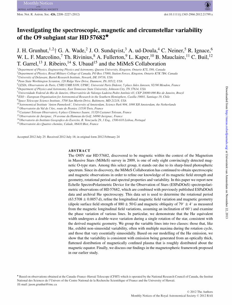
Figure 1. Selected regions of visible spectra from ESPaDOnS. Spectra at different rotational phases are shown to highlight the observed variability in almostall lines (0.02 – solid black, 0.30 – dashed red, 0.45 – dotted blue, 0.72 – dash–dotted green; see Section 6 for further details). The ions with the most significantcontribution to each line are also labelled.

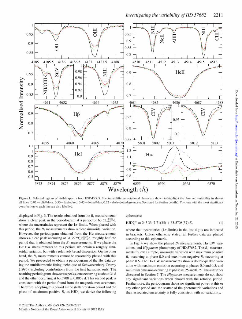
displayed in Fig. 3. The results obtained from the B� measurementsshow a clear peak in the periodogram at a period of 63.52+0.18

−0.17 d,where the uncertainties represent the 1σ limits. When phased withthis period, the B� measurements show a clear sinusoidal variation.However, the periodogram obtained from the Hα measurementsshows a clear peak occurring at 31.7929+0.0029

−0.0014 d, roughly half theperiod that is obtained from the B� measurements. If we phase theHα EW measurements to this period, we obtain a roughly sinu-soidal variation, but with a relatively broad dispersion. On the otherhand, the B� measurements cannot be reasonably phased with thisperiod. We proceeded to obtain a periodogram of the Hα data us-ing the multiharmonic fitting technique of Schwarzenberg-Czerny(1996), including contributions from the first harmonic only. Theresulting periodogram shows two peaks, one occurring at about 31 dand the other occurring at 63.5708 ± 0.0057 d. This second peak isconsistent with the period found from the magnetic measurements.Therefore, adopting this period as the stellar rotation period and thephase of maximum positive B� as HJD0 we derive the following

ephemeris:

HJDmaxB�

= 245 3347.71(35) + 63.5708(57) E, (1)

where the uncertainties (1σ limits) in the last digits are indicatedin brackets. Unless otherwise stated, all further data are phasedaccording to this ephemeris.

In Fig. 4 we show the phased B� measurements, Hα EW vari-ations, and Hipparcos photometry of HD 57682. The B� measure-ments follow a simple, sinusoidal variation with maximum positiveB� occurring at phase 0.0 and maximum negative B� occurring atphase 0.5. The Hα EW measurements show a double-peaked vari-ation with maximum emission occurring at phases 0.0 and 0.5, andminimum emission occurring at phases 0.25 and 0.75. This is furtherdiscussed in Section 7. The Hipparcos measurements do not showany significant variations when phased with the rotation period.Furthermore, the periodogram shows no significant power at this orany other period and the scatter of the photometric variations andtheir associated uncertainty is fully consistent with no variability.



msterdam

on Novem



ownloaded from




Figure 2. Mean LSD Stokes V (top), diagnostic null (middle) and Stokes Iprofiles (bottom) of HD 57682 from observations obtained at four differentrotational phases (see Section 3; 0.02 – solid black, 0.30 – dashed red, 0.45– dotted blue, 0.72 – dash–dotted green). The V and N profiles are expandedby the indicated factor and shifted upwards, and smoothed with a 3-pixelboxcar for display purposes. A clear Zeeman signature is detected at mostphases in the Stokes V profiles, while the null profile shows no signal. Theintegration limits used to measure the longitudinal field are indicated by thedotted lines and the mean 1σ pixel uncertainty for each profile is also shown.

Table 2. Journal of spectroscopic observations listing the iden-tification of the data set, the typical resolving power of the in-strument, the epoch of the observations, the number of spectraobtained within the given data set, the resulting number of dis-tinct observations and the median per pixel S/N in the Hα regionfor the data set.

Res. Num Num MedianName power Epoch spec obs S/N

CES 45 000 1996 7 7 540UVES 50 000 2002 8 1 160FEROS 48 000 2004 5 5 170

LCO 40 000 2009 10 3 360BeSS 15 000 2008–2011 51 51 70

Table 3. Spectroscopic Hα EW measurements. Included is theinstrument or observatory name, the heliocentric Julian date andthe measured Hα EW and its corresponding 1σ uncertainty.Shown here is only a sample of the table. The full table canbe found in Appendix A.

Data set HJD Hα EW (Å) σEW (Å)

CES 245 0125.6216 1.270 0.014CES 245 0126.6291 1.108 0.007CES 245 0127.6296 0.926 0.008CES 245 0128.6284 0.735 0.012CES 245 0129.6287 0.569 0.011CES 245 0130.6194 0.454 0.010

4 ROTAT I O NA L B ROA D E N I N G

Grunhut et al. (2009) measured the projected rotational velocity(v sin i) using the Fourier transform method (e.g. Gray 1981; Jankov1995; Simon-Dıaz & Herrero 2007). They compared the positionsof the first nodes in the Fourier spectrum to a theoretical Gaussianprofile convolved with a rotationally broadened profile correspond-ing to a particular v sin i, and found a v sin i = 15 ± 3 km s−1.

If we assume rigid rotation and take the radius as inferred byGrunhut et al. (2009) (R� = 7.0+2.4

−1.8 R�) and the period obtained inthis work (P = 63.5708 d), we find a maximum allowed v sin i (i.e.for sin i = 1) ∼7.5 km s−1, which is inconsistent with the resultsobtained from the Fourier analysis. This implies that contributionsfrom non-rotational broadening, as noted by Grunhut et al. (2009),significantly affect the Fourier spectrum resulting in the incorrectinterpretation of the first node representing the rotational broaden-ing.

In our endeavour to constrain the rotational broadening, we re-analysed the spectra, particularly focusing on those obtained atphases where the lines appeared their narrowest and therefore wereleast affected by macroturbulence (see Section 6 for further de-tails). We identified lines from a theoretical SYNTH3 (Kochukhov2007) spectrum for which the resulting Fourier spectrum was min-imally affected when significant contributions of macroturbulencewere included. We then compared the Fourier spectrum obtainedfrom a theoretical profile with 5 km s−1 rotational broadening tothat obtained from the observed spectrum and measured the differ-ence between the positions of the first nodes to obtain the v sin iof the spectral line. Using this procedure on several lines from thespectrum obtained on 2009 December 31 indicate a v sin i = 6.1 ±1.9 km s−1, consistent with the range implied by the rotation pe-riod and estimated radius of HD 57682. However, we note that thisperiod is sufficiently imprecise that it cannot be used to usefullyconstrain the inclination of the rotation axis. We also found thatthe C IV λ5801 line was one of the lines least affected by the addi-tion of macroturbulence and therefore also used this single line todetermine a unique v sin i, as illustrated in Fig. 5. From measure-ments of this line at several rotation phases we find a best-fittingv sin i = 4.6 ± 0.6 km s−1, where the uncertainties represent the 1σ

limits. Given the range of v sin i obtained from the C IV λ5801, ouradopted R� and Prot, implies that i ∼ 56◦+35◦

−23◦ , or that we can placea lower limit on i such that i > 30◦, at a 1σ confidence. However,at ∼4.6 km s−1 we are approaching the spectral resolution of ES-PaDOnS (∼4.4 km s−1) and therefore one must be cautious to notoverinterpret these results.

5 M AG N E T I C FI E L D G E O M E T RY

The magnetic field geometry of HD 57682 was investigated assum-ing the field is well described by the oblique rotator model (ORM),which is characterized by four parameters: the phase of closest ap-proach of the magnetic pole to the line-of-sight φ0; the inclination ofthe stellar rotation axis i; the obliquity angle between the magneticaxis and the rotation axis β and the dipole polar strength Bd. Thismodel naturally predicts the simple sinusoidal variation of the lon-gitudinal magnetic field measurements as shown in Fig. 4, implyingthat the longitudinal field curve of HD 57682 is well described by asimple dipole topology of its global magnetic field.

We first attempted to infer the characteristics of the magneticfield based on the B� measurements. These measurements are nearlysymmetric about 0 and we can therefore infer that either i or β (orboth) are close to 90◦. This is similar to the B� variation of β Cephei(e.g. Donati et al. 2001), and similar to this star, Bd and β are wellconstrained except as i approaches 0◦ or 90◦. As i approaches 0◦,Bd becomes unconstrained, while as i approaches 90◦, β becomesunconstrained. To infer the characteristics of the magnetic field, wecarried out a χ2 minimization, comparing the observed B� curve toa grid of computed longitudinal field curves to determine Bd and β

for a fixed linear limb darkening coefficient of 0.35 (Claret 2000)and various fixed inclinations.



msterdam

on Novem



ownloaded from




Figure 3. Periodograms obtained from the B� measurements (solid black)and from the Hα EW variations including contributions from the first har-monic (dashed red). Note the strong power present in the Hα periodogramat P = 31.7927 d but the lack of power from the B� measurements at thisperiod. However, a consistent period is found at P = 63.5708 d from bothdata sets.

The resulting χ2 distributions from our fits are shown in Fig. 6.For an assumed i = 60◦ we find that Bd = 880 ± 50 G and β = 79◦ ±4◦. If we take i = 30◦, we infer that Bd = 1500 ± 90 G and β =86◦ ± 2◦, which places an upper limit on the dipole field strength ifi > 30◦ as implied from the constraints derived in Section 4. Alsoshown in Fig. 6 are χ2 distribution for other inclinations to illustratehow the distribution varies as a function of inclination.

We also attempted to constrain the magnetic field characteristicsbased on fits to the individual LSD Stokes V profiles by comparingour profiles to a large grid of synthetic profiles, also characterizedby the ORM. The models were computed by performing a disc

Figure 5. Fourier spectrum of the C IV λ5801 line solid black compared to atheoretical line profile with v sin i = 5 km s−1 with an additional macrotur-bulent velocity of 20 km s−1 dashed red, which we find necessary to providea good fit to the observed line profile. The difference in the positions of thefirst nodes (as indicated by the vertical dotted lines) is used to determine thebest-fitting v sin i = 4.2 km s−1 for this observation.

integration of local Stokes V profiles assuming the weak field ap-proximation and uniform surface abundance. The parameters of theStokes V profiles were chosen to provide the best fit to the widthof the average of all the observed I profiles, and the best fit to thedepths of each individual observed I profile. For each observationwe found the parameters that provided the lowest χ2 value andinferred the maximum likelihood by combining these results in aBayesian framework.

We conducted our fits for varying inclinations and found thatthe maximum likelihood model for i ∼ 80◦ provided the low-est combined total χ2, but this value was not significantly dif-ferent from those obtained for other inclinations. However, as i in-creased we did find increasing deviations between the best B�-fit and

Figure 4. Phased observational data using the ephemeris of equation (1). Upper: longitudinal magnetic field variations measured from LSD profiles of theESPaDOnS spectra. Middle: Hα EW variations measured from ESPaDOnS (black circles), CES (red squares), FEROS (blue Xs), Las Campanas Observatory(turquoise diamonds), UVES (pink up-facing triangles) and BeSS (green down-facing triangles) data sets. Lower: Hipparcos photometry. The dashed curve inthe upper frame represents a least-squares sinusoidal fit to the data.



msterdam

on Novem



ownloaded from




Figure 6. Reduced χ2 contours of dipole field strength Bd versus magnetic obliquity β permitted by the longitudinal field variation of HD 57682 for varyinginclinations.

profile-fit model parameters; at i = 30◦ we found a best B�-fit β =86◦ and a profile-fit β = 80◦; at i = 80◦ we found a best B�-fit β =56◦ but β = 34◦ from the profile fits. We therefore conclude that weare unable to constrain the inclination from fits to the LSD profilesand continue to adopt i = 60◦ for the remainder of this discussionas this is the inclination inferred from the v sin i measurements andprovides similar magnetic parameters from both the B� and profilefits.

The maximum likelihood profile-fit model for i = 60◦ was foundwith Bd = 700 ± 30 G, where the uncertainty corresponds to the95.6 per cent significance level, and β = 68◦ ± 2◦, with the uncer-tainty corresponding to the 98.2 per cent confidence limits. Whilethe formal uncertainties are very low, we note that individual best-fitting parameters to each observation range from Bd ∼ 400–2000 Gto β ∼ 0◦–150◦. However, while the fits to Bd and β are not wellconstrained from fits to the individual observations at most phases,the maximum likelihood model is well constrained.

In Fig. 7 we compare the observed Stokes V profiles (grey circles)with the best profile-fit model for the given observation (dash–dotted blue), the maximum likelihood LSD model (dotted red) andthe model corresponding to the best-fitting parameters that wereobtained from the B� measurements for i = 60◦ (Bd = 880 G andβ = 79◦; solid green). The quality of the fits of the best-fittingand maximum likelihood models is similar, which shows that asingle dipole configuration can reasonably reproduce the observedStokes V profiles. However, systematic differences, particularly inthe wings of the profiles, are evident between the models and theobservations, resulting from the fact that our simple model cannotreproduce the extended wings in the observed I or V profiles. It isalso evident that the model corresponding to the best fit to the B�

curve does a poorer job of fitting the observed Stokes V profiles atseveral phases, possibly indicating that there may be an issue withthe way we chose to model the line profiles.

We investigated this potential issue by re-conducting our fits,but neglecting the varying line depths for each observation as wasdone in the original procedure. Instead we adopted a line depthas determined from the average of all our observations. From thenew fits for i = 60◦ we found a best-fitting Bd ∼ 900 G, which isconsistent with the results of the B� measurements. However, wefind a larger disagreement between the inferred magnetic obliquityas β was found to be ∼60◦. We also note that the overall combinedtotal χ2 value was slightly worse from these fits.

Another possibility is that the global magnetic topology containssignificant contributions from higher order multipoles. The B� curveis rather insensitive to these higher order moments, in contrast tothe velocity-resolved Stokes V profiles. We investigated this possi-

bility by applying our fitting procedure to a time series of syntheticprofiles calculated assuming our original dipole, supplemented bya significant aligned quadrupolar field moment. This model yieldsa longitudinal field curve essentially indistinguishable from thatproduced by the pure dipole. Our tests indicate that by trying tofit a pure dipole model to the dipole+quadrupole profiles, the pro-cedure would systematically infer dipole field strengths that werestrongly incompatible with the results obtained from the B� curve.Specifically, our tests showed a systematic overestimation of thedipole field strength at most phases. This trend is inconsistent withthe measurements presented in Fig. 7 and we therefore concludethat our polarimetric observations do not suggest any significantdetectable contributions from higher order multipoles.

6 LI NE VARI ABI LI TY

6.1 Equivalent width and radial velocity measurements

HD 57682 stands out from the sample of magnetic O-type stars dueto its sharp spectral lines and the apparently limited contamination ofits spectrum by wind and circumstellar plasma emission. Detectionand measurement of the line profile variations (e.g. Stahl et al.1996) can therefore be performed more sensitively for a much largersample of lines than for any other magnetic O-type star. It thereforerepresents a uniquely suited target for understanding the generalinfluence of magnetized winds of O-type stars on their spectrumand spectral variability.

To quantify the variability, we used the EW variations for numer-ous spectral lines. We also measured the radial velocities of eachspectral line by fitting a Gaussian to the cores of the profiles todetermine the central wavelength at each phase. A number of othermethods were investigated, but we ultimately settled on fitting thecores using a Gaussian as it provided less scatter in the measure-ments. However, since Hα displayed too much emission to carryout this fitting, we quantified the radial velocity of Hα by measuringthe centre of gravity (or centroid) of the line profile.

Our observations reveal that HD 57682 displays a rich varietyof line profile variability. In addition to the double-wave variationsof the Hα line discussed in Section 3, we observe variations inessentially every line present in the stellar spectrum, including otherH Balmer lines, lines of neutral and ionized He and lines of metals:C III and C IV, N III, O II, Mg II and Si III and Si IV. The EW and radialvelocities of all lines vary coherently when phased according to therotational ephemeris (equation 1).

The line variations can be approximately grouped into two cat-egories. The first represents lines (mostly metals and some neutral



msterdam

on Novem



ownloaded from




Figure 7. Mean circularly polarized LSD Stokes V profiles (grey circles). The error bars represent the 1σ uncertainties of each pixel. Also shown are theindividual best-fitting model profiles for each phase (dash–dotted blue), the model that provides the global maximum likelihood (dotted red; Bd = 700 G, β =68◦) and the model corresponding to the best fit to the B� measurements (Bd = 880 G, β = 79◦; solid green), all for an assumed inclination of 60◦. The phaseand best-fitting parameters of the individual observations are also indicated.

He lines) with EW measurements that vary sinusoidally, as dis-played in Fig. 8. The second includes those, like Hα, that displayEW phase variations that are distinctly non-sinusoidal (as shown inFig. 9), and likely directly reflect, to varying degrees, the variableprojection of the flattened equatorial magnetospheric plasma den-sity enhancement, as further discussed in Section 7. These groupsare discussed in more detail below.

Except for C IV λλ5801, 5812, all lines with sinusoidally vary-ing EW measurements show minimum emission (or maximum ab-sorption) at about phase 0.0 and maximum emission (or minimumabsorption) at phase 0.5. At phase 0.5, these lines are shallowerand broader than at phase 0.0, as illustrated in Fig. 1. The differ-ence in line width and depth is quite significant. Most lines have anextended red wing at phase 0.5 that disappears at phase 0.0.

The Hα line shows variable emission with two maxima per ro-tation cycle. The phases of the emission extrema, 0.0 and 0.5, cor-

respond to the phases of longitudinal magnetic field extrema andtherefore closest approach of the magnetic poles to the line-of-sight. In addition, the Hα EW curve exhibits two emission minimaat phases 0.25 and 0.75, corresponding to the phases where the mag-netic equator crosses the line-of-sight. These phenomena are usuallyinterpreted (e.g. Donati et al. 2001) as the consequence of the vari-able projection of a flattened distribution of magnetospheric plasmatrapped in closed loops near the magnetic equatorial plane, andpossibly the occultation of the stellar disc by this plasma at phases0.25 and 0.75. Only three other lines – He I λ5876, He II λ4686and Hβ (see Fig. 9) – show clear evidence of similar reversals atphases 0.25 and 0.75, although a marginal contribution is suspectedfor He I λ4921 and He I λ4471. The emission level in Hα at phase0.5 is roughly 10 per cent larger than at phase 0.0. Likewise, theemission minimum at phase 0.75 appears 20 per cent less than thecorresponding emission minimum at phase 0.25. However, these



msterdam

on Novem



ownloaded from




Figure 8. Rotationally phased EW measurements (top panels) and radial velocity measurements (bottom panels) for selected spectral absorption lines thatappear to have sinusoidally varying EW measurements. Note that while the EW variations of Hγ are consistent with the other lines, the radial velocity variationsare out of phase with the rest of the lines. Least-squares sinusoidal fits to the data are also shown (dashed curves).

measurements are primarily measured from BeSS spectra with lim-ited S/N.

In almost all the spectral lines that show sinusoidally varyingphased EW measurements, we find approximately sinusoidallyvarying radial velocity measurements. These variations reach amaximum radial velocity between phases 0.2 and 0.3 and showa peak-to-peak amplitude of about 2 km s−1, with a mean radial ve-locity of ∼22 km s−1. This is not the case for Hγ , which reaches amaximum radial velocity at phase 0.0 and minimum at phase 0.5,and shows a peak-to-peak difference of ∼8 km s−1. Other than Hβ,we see non-sinusoidal variations in the radial velocity measure-ments for the lines that show clear, non-sinusoidal EW variations,which often mirror the EW variations with maximum radial veloc-ity occurring at minimum emission and minimum radial velocityoccurring at maximum emission. The radial velocity measurementsfor Hβ phase in a similar manner with Hγ – they are nearly si-nusoidal, reach maximum radial velocity at phase 0.0 and appearflat-topped.

6.2 Line profile variations

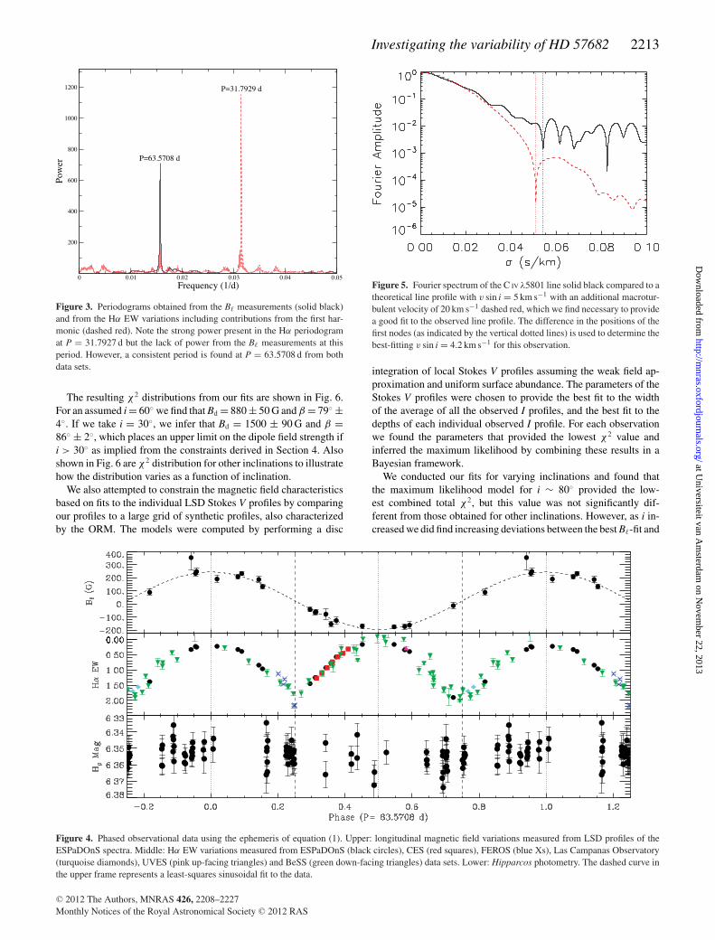
In Figs 10 and 11 we plot the phased line profile variations, ordynamic spectra. In these figures, we have subtracted the profileobtained on 2010 December 24 to highlight the variability. Thisspectrum was obtained at phase 0.72 and corresponds to the obser-vation where the magnetic equator is passing our line-of-sight and,as previously discussed, when the flattened distribution of magneto-spheric plasma is viewed nearly edge-on, and therefore provides thelowest contribution of emission. Our dynamic spectra indicate thata single pseudo-emission feature (a feature that appears in emissionrelative to the 2010 December 24 profile) occurs once per cycle, andis centred at phase 0.5 in the dynamic spectra of the lines with si-nusoidally varying EW measurements (Fig. 10). In almost all theselines, we find that the pseudo-emission is mostly confined to the in-ner core region and extends further out in the blue wing than the redwing. During phases of maximum emission we also find increasedpseudo-absorption in the red wing, except for He I λ4471, which



msterdam

on Novem



ownloaded from




Figure 8 – continued

does not appear to show additional pseudo-absorption, but doesshow strong evidence of pseudo-emission during phases of maxi-mum absorption, which is centred at phase 0.0. Other lines showvarying amounts of pseudo-emission during this phase as well, butthis feature is most prominent in the He lines shown in Fig. 10.

The dynamic spectra for the C IV lines appear different. Maximumemission still occurs once per cycle, centred at phase 0.5, but theemission feature is mainly constrained to the inner core region anddoes not extend into the blue wing as it does for other lines. Duringphases of maximum emission, there appears to be an increase inpseudo-absorption in both wings, but the absorption in the red wingappears stronger. A similar dynamic spectrum is also found for theHe II λ4686 line, as shown in the left-hand panel of Fig. 11. In almostall the lines shown in Figs 10 and 11 we find that the features allappear at low velocities with the centres of the features increasingin velocity with increasing phase. However, this does not appear tobe the case with the He lines, which appear more symmetric, exceptfor the extended pseudo-absorption into the blue wing, which islikely caused by the forbidden transitions in these He lines.

In Fig. 12 we show the dynamic spectra of the other lines withnon-sinusoidally varying EW variations. A non-local thermody-namic equilibrium (NLTE) TLUSTY (Lanz & Hubeny 2003) syntheticprofile was subtracted from the Balmer lines in this figure to high-light the circumstellar emission contribution. As was found in theEW variations, we see two emission features per rotation cycle, onecentred around phase 0.0 and the other centred around phase 0.5.In the He I λ5876, Hγ and Hβ line we find the lines to be mainlyin absorption and the emission feature at phase 0.0 to be narrowerand weaker in emission than the feature at phase 0.5. In the He I

line shown, both emission features appear redshifted with respectto the systemic velocity of HD 57682; the narrower feature is foundto have a central velocity of ∼75 km s−1 while the broader featurehas a central velocity of ∼65 km s−1. There also appears to be an

additional weak emission feature that is blueshifted with respect tothe systemic velocity occurring at phase 0.0. Hβ and Hγ appearsimilar to the He I λ5876 line. Both show a strong and broad emis-sion feature at phase 0.5, and a weaker, narrower emission featureat phase 0.0. This is not the case for Hα, which shows both emissionfeatures with nearly the same width and same emission level; it isevident that the strength of the weaker emission feature at phase 0.0is decreasing for higher Balmer lines. Unlike the He I λ5876 line,the emission features of the Balmer lines have their central veloci-ties alternating about the systemic velocity; the feature at phase 0.0appears blueshifted, while the feature at phase 0.5 is redshifted.

7 C I R C U M S T E L L A R E N V I RO N M E N T

7.1 Magnetosphere

As discussed in the previous section, the Hα emission variation isoften qualitatively attributed to the variable projection of a flatteneddistribution of magnetospheric plasma trapped in closed loops nearthe magnetic equatorial plane. To this end, we explored the potentialof using a ‘Toy’ model, similar to that described by Howarth et al.(2007), to fit the observed Hα EW variations. This model assumesthat the Hα emission is formed in a centred, tilted, infinitely thin,optically thick disc, in which the relative emission is only a functionof the projected area of the disc, taking into account occultation bythe star. We are only able to model the relative emission, but ourmodel indicates that if we assume the inclination angle betweenthe disc axis and the rotation axis (α) is the same as the magneticobliquity (β) then only subtle variations are predicted in the EWcurve for different inclinations (assuming the relationship betweeni and β is constrained by the ORM), which are indistinguishablewith the precision of our current measurements. We also find thathigher α values provide much better fits and therefore we adopt



msterdam

on Novem



ownloaded from




Figure 9. Rotationally phased EW measurements (top panels) and radial velocity measurements (bottom panels) for selected spectral absorption lines withclearly non-sinusoidal EW variations. Hα measurements from ESPaDOnS (black circles), CES (red squares), FEROS (blue Xs), Las Campanas Observatory(turquoise diamonds), UVES (pink up-facing triangles) and BeSS (green down-facing triangles) data sets. The BeSS Hα radial velocity measurements areshown as grey triangles. The large scatter of these measurements with respect to the other data sets likely results from their poor S/N and low spectral resolution.

the α = β = 79◦ as derived from the B� measurements as our discinclination. Using this value, we first attempted to constrain the discradii but realized that the inner (Rin) and outer (Rout) radii of thedisc are poorly constrained by the precision of our observations.However, a best-fitting Rin = 1.3 ± 0.3 R� and Rout = 1.8+0.3

−0.2 R�

(as measured from the centre of the star, i.e. a distance of 0.3 ±0.3 R� and 0.8+0.3

−0.2 R� from the stellar surface) are found, where theuncertainties represent the 1σ limits. An illustration of this modelis presented in Fig. 13.

A comparison between the predicted EW variations from our‘Toy’ model and the observed EW variations is shown in Fig. 14.As illustrated, the model is able to qualitatively reproduce the gen-eral features of the observed EW variations including the sharpemission minima, the smooth variation during maximum emissionand the double-peaked nature of the variability, suggesting that theHα emission does form in an optically thick, flattened distribution

of circumstellar plasma with a disc-like structure. However, ourmodel predicts a lower emission level between phases 0.0–0.25 and0.75–1.0 and a higher emission level between phases 0.25–0.4 and0.6–0.75 than observed, and there is a visible offset between thephases of emission minima; our model predicts the minima to occurat phases 0.23 and 0.77, not 0.25 and 0.75 as observed. To inves-tigate these discrepancies, we conducted another search allowingthe disc axis inclination to vary. Our results show that α = 88◦ ±1◦ (and a corresponding Rin = 1.0 R� and Rout = 1.6 R�) provides abetter overall fit to the observations, but is inconsistent with our de-rived value of β. This disc orientation is better able to reproduce theemission level throughout the rotation cycle and correctly predictsthe phases of minimum emission as illustrated in Fig. 14.

In addition to investigating the magnetospheric properties via the‘Toy’ model, we also used the method of Sundqvist et al. (2012)to study the Hα variability. Sundqvist et al. (2012) showed that



msterdam

on Novem



ownloaded from




Figure 10. Phased variations in selected spectral lines with sinusoidal EW variations. Plotted is the difference between the observed profiles and the profileobtained on 2010 December 24 (dashed-red, top panel), which occurred at phase ∼0.75, corresponding to when the magnetic equator crosses the line-of-sight.

in a slow rotator such as HD 57682, the transient suspension ofwind material in closed magnetic loops, which is constantly fedby the quasi-steady wind outflow, leads to a statistically overdense,low-velocity region in the vicinity of the magnetic equator that

causes persistent, periodic variations of Balmer lines. This methodutilizes the two-dimensional (2D) magnetohydrodynamics (MHD)wind simulations of ud-Doula, Owocki & Townsend (2008) andthe magnetic parameters determined from the B� measurements to



msterdam

on Novem



ownloaded from




Figure 10 – continued

Figure 11. Same as Fig. 10 but for selected spectral lines with clearly non-sinusoidal EW variations or EW variations that appear antiphased with the otherlines. Plotted is the difference between the observed profiles and the profile obtained on 2010 December 24 (dashed-red, top panel), which occurred atphase ∼0.75, corresponding to when the magnetic equator crosses the line-of-sight.

determine the properties of the magnetically confined plasma. Wenote however that the original MHD models were computed for anO-type supergiant. Therefore, in the Hα synthesis here, we havesimply re-scaled the Hα scaling invariant Q = (Mf 2

cl)/(v∞ R�)3/2

(Puls, Vink & Najarro 2008) from the original simulation to thevalue obtained for HD 57682 using the parameters of Grunhut et al.(2009). These properties are then used to synthesize the expectedHα line profile as viewed from our line-of-sight as the star ro-tates. Unlike the ‘Toy’ model, these simulations are sensitive to theadopted mass-loss rate. We characterize the mass-loss rate as theproduct of the stellar mass-loss rate and the square root of a windclumping factor, which we assume to be about 4–10 as suggestedby several recent studies (e.g. Bouret et al. 2003; Najarro, Hanson& Puls 2011; Sundqvist et al. 2011a). We attempted to constrainthe wind properties by fitting the observed Hα profile during phasesthat have the lowest contributions from the disc emission. As al-ready noted by Grunhut et al. (2009), we cannot fit the Hα profileusing a mass-loss rate as derived from the ultraviolet (UV) lines(log M ∼ −8.85 M� yr−1). The additional emission resulting from

the wind is too low at phase 0.25 or 0.75 (minimum emission),which results in a line profile that is mainly in absorption, contraryto what is actually observed (see Fig. 15).

Our results (based on fits to the Hα profile) suggest that the lackof emission is either due to an underestimated stellar mass-lossrate (by a factor of 10–30), or that the wind is very clumpy (notethat clumping was not taken into account in the study of Grunhutet al. 2009). This is consistent with many recent studies that findlarge discrepancies between UV and optical mass-loss rates (seeSundqvist, Owocki & Puls 2011b, and references therein). Further-more, according to Figs 16 and 17, we find that the model using theUV-derived mass-loss rate produces little to no emission with anysignificant variability. In fact, the amplitude and the offset of theEW variations shown in Fig. 16 are very sensitive to the adoptedmass-loss rate. If we choose a mass-loss rate that best fits the profilesat minimum emission phases, we obtain a mass-loss rate of ∼15times the suggested UV mass-loss rate (see Fig. 15). However, whilethe predicted minimum emission of the EW variations is well fit,the maximum emission is underestimated. A mass-loss rate of ∼20



msterdam

on Novem



ownloaded from




Figure 12. Same as Fig. 10 but for spectral lines that show evidence of two emission features per rotation cycle. The Balmer lines are plotted as the differencebetween the observed profiles and a NLTE TLUSTY model profile (top panel, dashed-red) to highlight the circumstellar emission. The He I λ5876 lines is plottedas the difference between the observed profiles and the profile obtained on 2010 December 24 (dashed-red, top panel).

Figure 13. Illustration of our ‘Toy’ model for the Hα emission disc. The left-hand panel provides an example schematic diagram showing the orientation ofthe plane of the disc for a given disc inclination α relative to the rotation axis. The other panels represent projections of the disc (solid black) and central star(solid red) on to our line-of-sight during phases 0.0, 0.33 and 0.66. The thin green arrow in these panels represents the projected rotation axis relative to therotation axis (taken to be 60◦), while the thick blue arrow represents the disc axis of 79◦ relative to the rotation axis.



msterdam

on Novem



ownloaded from




Figure 14. ‘Toy’ model compared to phased Hα EW measurements (blackcircles). The solid red curve represents a model with an α = 79◦ between therotation axis and the disc axis, as inferred from the fits to the B� variations,while the dashed blue curve represents the best-fitting model with an α =88◦. Both models assume i = 60◦.

Figure 15. Comparison between observed Hα profile (solid black) from2010 December 24, corresponding to a phase of 0.72, and synthetic profilesfollowing the procedure of Sundqvist et al. (2012) at this same phase. Themodel profiles were created with an adopted mass-loss rate as determinedby Grunhut et al. (2009) (dotted blue), a mass-loss rate of 17 (solid green)and 21 times this value (dashed red).

times the previous estimate provides a better fit to the EW variations,by underestimating the maximum emission and overestimating theminimum emission. A mass-loss rate of ∼30 times the previouslyestimated value is needed to provide the correct amplitude of the EWvariation, but, as the wind emission is predicted to be significantlyhigher, there exists a significant offset between the predicted andobserved EW values. In any case, our MHD simulations indicatethat a higher mass-loss rate than derived by Grunhut et al. (2009)is necessary in order to observe significant variability, with similarcharacteristics to the observed Hα dynamic spectrum (Fig. 17). Thecharacteristics of the MHD EW curves are similar to the predic-tions of our ‘Toy’ model; the phasing of minimum emission is notat phases 0.25 and 0.75 and the relative amplitude of the emissionis slightly lower when using α = 79◦ (note that the pseudo-discnaturally forms along the magnetic equator in these MHD simula-tions, i.e. α = β). Just as was found with the ‘Toy’ model, a higher

Figure 16. Comparison between the measured EW variations of HD 57682(black circles) and the theoretical EW variations of our MHD model fordifferent mass-loss rates as labelled (UV corresponds to the UV mass-lossrate derived by Grunhut et al. 2009). While the absolute EW variations ofthe M/M� = 30× UV (dash–dotted blue) model do not fit the observedEW curve, the amplitude of the predicted variations from this model doesprovide a good fit, as illustrated for the same model but vertically shifted tobetter match the variations implied by the observations (black dotted line).

β = 88◦ provides a better agreement with observations. Of partic-ular interest, is the fact that the synthesized emission variation inFig. 17 is predicted to be symmetric about the systemic velocityof HD 57682 with the adopted high β. However, a lower β doesprovide increased occultation of the disc and therefore necessarilyresults in a more asymmetric line profile variation at some phases,similar to the observations.

7.2 Greater circumstellar region

We continued our investigation of the circumstellar environment tolarger distances as probed at IR wavelengths. Our original intentionwas to investigate the IR properties of HD 57682’s SED to addressthe uncertain classification of HD 57682 as a classical Oe star andto potentially probe the extent of the magnetosphere.

In Fig. 18, we show the SED of HD 57682 from the UV to IRwavelengths. The data were collected from the IUE data base and theavailable photometric archives discussed in Section 2. Also includedin this figure are theoretical SEDs based on the original stellarparameters of Grunhut et al. (2009) and updated values presentedhere. A comparison between our CMFGEN (Hillier & Miller 1998)model with the newly inferred parameters and the IUE data is alsopresented in the lower panel of this figure, illustrating the agreementbetween the observations and the model. We note that we have stilladopted the lower UV mass-loss rate of Grunhut et al. (2009) inthis CMFGEN model. Our new model has revised the distance andreddening parameters of Grunhut et al. (2009, d ∼ 1.3 kpc, E(B −V) = 0.07), which were only derived from the IUE data and do notprovide a good fit to the photometric measurements blue-ward of50 000 Å (5 µm). Our revised parameters are d ∼ 1.0 kpc and E(B −V) = 0.12. The SED also shows a large disagreement between theIRAS and WISE data points, but this reflects the variation in theaperture sizes of the different instruments; the IRAS aperture isabout five times larger and therefore includes more contributionof circumstellar emission (as further discussed below), while theWISE measurements represent more of the true ‘stellar’ flux, and



msterdam

on Novem



ownloaded from




Figure 17. Rotationally phased variations in observed (right-hand panel) and modelled Hα profiles. The model in the left-hand panel shows the predictedvariations assuming the mass-loss rate of Grunhut et al. (2009), while the central panel uses an adopted mass-loss rate of 21 times this value. Note the lack ofpredicted variations of the model adopting the mass-loss rate of Grunhut et al. (2009) and the predicted emission symmetry.

Figure 18. Upper: observed IUE observations and IR flux measurementsfrom the indicated sources. Also included are stellar models correspondingto the parameters derived by Grunhut et al. (2009) (d = 1.3 kpc and E(B −V) = 0.07; dashed grey) and the revised model presented here (d = 1.0 kpcand E(B − V) = 0.12; dashed red). The larger flux of the IRAS data pointscompared to the WISE measurements reflects the significantly larger aper-ture and therefore increased contribution from the surrounding emission.Lower: comparison between the observed IUE spectrum (solid black) andthe CMFGEN model with the parameters inferred in this work (dashed red)in the wavelength range of 1380–1730 Å. The CMFGEN model still adoptsthe lower mass-loss rate of Grunhut et al. (2009) and not the higher valueneeded to fit Hα (Fig. 15; see Section 7 for further discussion). Both themodel and observed spectrum were smoothed for display purposes.

appear consistent with the other IR measurements. The observedSED does show a large disagreement with the theoretical SED formeasurements red-ward of 1 × 105 Å (10 µm). The observed IRemission appears to be increasing with increasing wavelength andnot decreasing as predicted by contributions from pure stellar flux,and therefore represents an additional source of emission.

In order to better understand the characteristics of the IR excesswe utilized the procedure of Ignace & Churchwell (2004) to modelthe free–free emission that would be emitted from a spherical cloud;IR excess is common amongst Be/Oe stars and is caused by free–free emission from the circumstellar disc. Using this procedure wefind that we can qualitatively match the characteristics of the IRexcess by varying the properties of the cloud. A brief investigationof this model shows that the location of the IR bump is mainlycontrolled by the temperature of the cloud (we find T ∼ 20 000 K tobe sufficient), but the size of the bump is controlled by the relativesizes of the cloud and star. For simplicity we assume that the cloudis of constant density, which then requires a cloud of approximately100 R� to reproduce the observations. If we instead adopt a cloudwith many large clumps of different densities and at different radii(as is done in Ignace & Churchwell 2004) we can achieve similarresults without the need for a 100 R� cloud. However, if we assumethat the cloud is not highly clumped and results from stellar masslost by HD 57682, this would imply an unreasonable mass for thecloud, suggesting that HD 57682 is in fact not a classical Oe star.

In light of this conclusion we further investigated the IRAS pho-tometry. In the end we suspect that the additional emission is a resultof HD 57682’s illumination of the IC 2177 nebula (Halbedel 1993).A look at the HIRES/IRAS maps, as shown in Fig. 19, shows signif-icant IR emission centred on HD 57682 at 25 and 60 µm, with thesize of the emission cloud larger at 60 µm. Emission is also evidentat 12 µm, but does not reach the same spatial extent as found at 25or 60 µm. At 100 µm the cloud overwhelms the field of view (30 ×30 arcmin2), but appears to be a blend of several clouds. It is alsoevident from these images that the majority of the point sources inthe field of view are illuminating the nebula at these wavelengths,further corroborating our suggestion that the IR emission does notresult from a circumstellar disc or even the extended magnetosphereof HD 57682.



msterdam

on Novem



ownloaded from




Figure 19. IR emission as detected by IRAS/HIRES at different wavelengths(top left – 12 µm; top right – 25 µm; bottom left – 60 µm; bottom right –100 µm). Each image represents a 30 × 30 arcmin2 scale. Point sources areindicated by the red circles and the field of view is centred on HD 57682.Note that the elliptical shape of the point sources is a result of the scanningdirection of the IRAS detector.

8 D I S C U S S I O N A N D C O N C L U S I O N S

In this paper we report on our ongoing work towards understandingthe magnetic properties and variability of the magnetic O9 subgiantstar HD 57682. Our current analysis is based on an extensive dataset spanning almost 15 yr, including archival spectra from ESO’sCES, UVES and FEROS spectrographs, and from the echelle spec-trograph at LCO. In addition numerous low-resolution spectra wereacquired and accessed from the BeSS data base. Furthermore, wealso present 13 newly obtained, high-resolution spectropolarimet-ric observations acquired with ESPaDOnS at the CFHT within thecontext of the MiMeS project.

A period analysis performed on the spectroscopic Hα EW vari-ations and the polarimetric B� measurements resulted in a single,consistent period between the polarimetric and Hα variations of63.5708 ± 0.0057 d, which we infer to be the rotational period ofthis star. This long rotational period suggests that the v sin i inferredby Grunhut et al. (2009) is too high by a factor of ∼2, which ledus to attempt to remeasure this value. We found that the C IV λ5801photospheric line was the least susceptible to additional macrotur-bulence in the line profile and therefore we were able to estimatea new v sin i = 4.6 ± 0.6 km s−1, which is now consistent withthe ∼63 d period. This period also implies that the inclination of therotation axis i > 30◦ with a best-fitting value i ∼ 56◦+34◦

−26◦ .From fits to the rotationally phased B� measurements we were

able to constrain the magnetic dipole parameters of HD 57682,assuming that the magnetic field is well characterized by the ORM.Taking i = 60◦, the data imply that Bd = 880 ± 50 G and β = 79◦ ±4◦. However, direct modelling of the individual mean LSD profilessuggests a somewhat weaker dipole field strength of ∼700–900 Gand a smaller obliquity angle of ∼60◦–68◦. However, the results arestrongly dependent on the adopted depth and width of the modelledLSD Stokes I and V profiles, as discussed in Section 5. Therefore, it

is likely that improved modelling of the observed line profiles thatcorrectly takes into account the profile variations could reduce thedisagreement and we therefore suggest that the real magnetic dipoleparameters are closer to the parameters implied by the B� variation.

The profile variations of nearly all observable lines in the high-resolution ESPaDOnS spectra were also investigated (Figs 8 and 9).Our analysis suggests that we can essentially separate all lines intoone of two categories as determined by the rotationally phased EWvariations of the spectral line. There are those lines that show clearevidence of double-peaked variations similar to Hα, while the restshow single-peaked, sinusoidal variations. The LPV of these lines,as described in Section 6, shows rotationally phased velocity vari-ations of the pseudo-absorption or pseudo-emission components,and the pattern of this variability is generally consistent amongst allthe lines.

In Section 7, we clearly showed that the double-peaked variationsof the Hα EW are well explained by the presence of the variable pro-jection of a flattened distribution of magnetospheric plasma trappedin closed loops near the magnetic equatorial plane. This flatteneddistribution is also predicted by MHD simulations using the stellarand magnetic properties as determined here and by Grunhut et al.(2009), although we find that a mass-loss rate that is 20–30 timesgreater than the value inferred by Grunhut et al. (2009) from the UVlines is necessary to produce the level of emission that is observed.However, at present we are not able to model UV resonance linesusing our MHD wind simulation and therefore must resort to mod-elling these lines using a spherically symmetric wind model. Thepredicted UV spectrum, as modelled using CMFGEN, indicates thepresence of several intense spectral emission lines that are observedmainly in absorption in the IUE spectrum (e.g. Si IV λ1400 andN IV λ1718) or that the observed lines are too weak (e.g. N V λ1240and C IV λ1550). However, the IUE spectrum is well reproducedwhen adopting the lower mass-loss rate, as already demonstratedby Grunhut et al. (2009) and illustrated in the lower panel of Fig. 18.Note that CMFGEN assumes a spherically symmetric wind, whereasthe MHD wind simulations predict a highly non-spherical wind withimportant consequences for spectral line diagnostics (ud-Doula &Owocki 2002; Sundqvist et al. 2012). Furthermore, the UV linesare very sensitive to the ionization structure of the wind, which mayalso be largely affected by a non-spherically symmetric wind. Thisis not the case for Hα as it is a recombination-based optical emissionline, which is insensitive to the exact modelling of the ionizationstructure (e.g. Sundqvist et al. 2012). Therefore it is not surprisingthat there is a disagreement between the mass-loss rates inferred byour optical and UV analyses. Future MHD UV line modelling willbe necessary to resolve this discrepancy.

The MHD model provides not only an independent analysis ofthe stellar mass-loss rate, but also of the magnetic geometry, whichis constrained by the characteristics of the Hα EW variations. Usingthe higher mass-loss rate shows that the Hα emission variation canbe reasonably modelled, however, there are several inconsistenciesbetween the models and observed data that reflect our uncertaintyin the mass-loss rate and potentially the magnetic geometry. Our re-sults show that the inclination of the disc relative to the rotation axismust be greater than the inferred magnetic obliquity (as measuredfrom our polarimetric data), since a higher disc inclination providesa much better fit to the observed EW variations. This may also beattributed to warping of the disc, or may even reflect the fact thatthe disc does not necessarily lie in the magnetic equatorial plane aspredicted by MHD simulations.

As with the LPV for the sinusoidally varying lines, there alsoappears to be rotationally phased velocity variations in the position



msterdam

on Novem



ownloaded from




of the central emission component in the Hα line profile that is notpredicted by the MHD simulations. We discuss a few potential ex-planations. If the disc structure is not vertically symmetric along therotation axis (i.e. not symmetric about the equatorial rotation plane)the resulting line profiles would be asymmetric and would result invelocity shifting of the disc emission. Likewise, enhanced emissionfrom a non-uniform velocity flow where the velocity flow occursat high magnetic latitudes could also explain our observations. Forexample, during phases where the disc is viewed nearly face on,the emission could appear systematically offset from the systemicvelocity if there is an additional outflow or inflow, for instance, dueto the stellar wind or circumstellar plasma falling back on to thestar. This would result in no velocity offset during phases where thedisc is viewed nearly edge on as the additional outflow or inflowwould appear perpendicular to our line-of-sight. However, it is dif-ficult to understand a scenario where there would be a preferencefor outflow or inflow of plasma at one magnetic hemisphere com-pared to the other. This is required to explain the velocity shiftingof the emission that occurs as our line-of-sight rotates from onemagnetic hemisphere to the other. Another possible solution is tointroduce an offset of the dipole relative to the centre of the star.Our preliminary tests suggest that a small offset of ∼0.2 R� alongthe rotation axis could explain the velocity shifting of the emissionthat is observed in Hα, although MHD models implementing thisoffset are necessary to confirm this phenomenon, which will be thesubject of future studies.

In addition to the LPV, we also measure RV variability in nearlyall spectral lines and find that all lines with sinusoidally varyingEW measurements show approximately sinusoidally varying RVmeasurements. Turner et al. (2008) investigated the binarity of thisstar and found no evidence of a companion in either their I-bandadaptive optics or RV measurements. If we assume that the RVvariations are due to a binary companion, a least-squares analysisof the RV measurements obtained from the mean LSD I profilewould suggest a mass function f (M/M�) = 2.2 ± 0.9 × 10−6 forthe companion star. For reasonable orbital inclinations, this wouldrequire the companion to be a very low-mass (and presumably a low-luminosity) star, and therefore should not have a significant effecton the observed line profile, which we clearly do observe. Takingthis into account, it is therefore unlikely that the RV variations aredue to a binary companion since we do not observe clear shifts ofthe entire spectroscopic lines. We propose that the RV variationsare likely a result of the variable asymmetry of the line profiles andsimply reflect the varying location of the centre-of-gravity in theprofiles. This is clearly evident in the lines that show a double-waveEW curve since the RV measurements also show a more complexdouble-wave pattern. Furthermore, there also appears to be moreof a direct relationship between the RV and EW measurements inthese lines, while the majority of the sinusoidally varying lines showa ∼0.25 phase offset between the RV and EW variations.

The root cause of the LPV in the sinusoidally varying lines is stillan outstanding issue. It is highly unlikely that these variations arecaused by surface features (e.g. chemical ‘spots’) as the observedvariability between multiple ions of a given species does not behaveas predicted by LTE or NLTE spectrum synthesis. For example, ourobservations demonstrate that the weak N IV λ4058 line exhibits thesame relative EW variation as the strong N III λ4523 line, but spec-tral modelling of these lines shows that the weaker line should show30 per cent stronger variation if due to abundance changes. Further-more, the strong Si IV λ4115 line and the weak Si IV λ4403 line shownearly the same level of EW modulation, but the weak Si IV lineshould show a 60 per cent larger amplitude in the EW variation if

resulting from abundance changes. The weak Si IV λ4667 line is alsopredicted to show the same relative EW variation as the λ4403 line,but our observations show a significantly greater level of variability(about 50 per cent larger) in the λ4667 line. Moreover, abundancespots require that all spectral lines of a given species vary in phase.This is clearly not the case for the C IV lines (5801, 5811 Å) that varyin antiphase with the C III lines (as shown in Fig. 8), or the N IV λ4058and N III λ4523 lines, which appear shifted relative to one anotherby a quarter of a cycle. The interpretation of the variability in termsof surface spots would also imply that all elements (except perhapsC) are concentrated at the same general region on the stellar surface,which would be a remarkable new phenomenon. Another possibilityis that the variations may result from pulsations; however, pulsationsshould occur on much shorter time-scales (e.g. Aerts, Christensen-Dalsgaard & Kurtz 2010). The rotationally phased, double-peakedEW variations are well explained by the variable projection of aflattened distribution of magnetospheric plasma, and at first glanceit is difficult to apply this same disc model to explain the variationsin the other lines. Occultation or variable emission from a symmet-ric disc would result in double-peaked variations in all lines andnot the single-peaked emission that we observe. However, the LPVof the higher Balmer lines (Fig. 12) likely provide the link betweenthe double-peaked variability and single-peaked variability; a de-crease in the strength of the emission feature at phase 0.25 and 0.75compared to the emission feature at phase 0 is clearly observed inhigher Balmer lines. Furthermore, this is also illustrated in the EWvariations of the Balmer lines (Figs 8 and 9), which show a cleartransition from the double-peaked EW curve at Hα to a single-peaked curve at Hγ . Therefore, we tentatively conclude that all lineprofile variability observed in HD 57682 is a result of variations ofthe flattened distribution of magnetospheric plasma. The details ofthe variable emission for different lines likely reflect the fact thateach line probes a different region of what is likely an asymmet-ric spatial or velocity distribution of the magnetospheric plasmaand that the disc is not completely optically thick for all lines-of-sight, for all wavelengths. We suspect that full three-dimensional(3D) MHD models and an extension of the line profile synthesistechniques of Sundqvist et al. (2012) to lines other than Hα arenecessary to properly model these properties.

In summary, the narrow-lined photospheric spectrum and weakwind of HD 57682 have allowed us to study its magnetic and mag-netospheric properties at a level of detail not currently achievablefor any other magnetic O-type star. The results of our analysis in-dicate a highly complex behaviour that can be used as a test bedfor future more sophisticated 3D MHD simulations to better un-derstand non-rotationally supported magnetospheres (also referredto as dynamical magnetospheres; Petit et al. 2011; Sundqvist et al.2012) of hot stars.

AC K N OW L E D G M E N T S

JHG acknowledges financial support in the form of an Alexan-der Graham Bell Canada Graduate Scholarship from the NaturalSciences and Engineering Research Council, and helpful discus-sions with C. P. Folsom. GAW acknowledges Discovery Grantsupport from the Natural Science and Engineering Research Coun-cil of Canada. JOS acknowledges support from NASA ATP grantNNX11AC40G. We thank Evgenya Shkolnik for reduction ofthe LCO observations. This work has made use of the BeSSdata base, operated at LESIA, Observatoire de Meudon, France(http://basebe.obspm.fr). The DENIS project has been partly fundedby the SCIENCE and the HCM plans of the European Commission



msterdam

on Novem



ownloaded from




under grants CT920791 and CT940627. It is supported by INSU,MEN and CNRS in France, by the State of Baden-Wurttemberg inGermany, by DGICYT in Spain, by CNR in Italy, by FFwFBWFin Austria, by FAPESP in Brazil, by OTKA grants F-4239 and F-013990 in Hungary and by the ESO C&EE grant A-04-046. Thisresearch has made use of the NASA/IPAC Infrared Science Archive,which is operated by the Jet Propulsion Laboratory, California In-stitute of Technology, under contract with the National Aeronauticsand Space Administration.

R E F E R E N C E S

Aerts C., Christensen-Dalsgaard J., Kurtz D. W., 2010, Asteroseismology.Springer-Verlag, Heidelberg

Bagnulo S., Landstreet J. D., Fossati L., Kochukhov O., 2012, A&A, 538,129

Bouret J.-C., Lanz T., Hiller D. J., Heap S. R., Hubeny I., Lennon D. J.,Smith L. J., Evans C. J., 2003, ApJ, 595, 1182

Bouret J.-C., Donati J.-F., Martins F., Escolano C., Marcolino W., Lanz T.,Howarth I. D., 2008, MNRAS, 389, 75

Claret A., 2000, A&A, 363, 1081Donati J.-F., Semel M., Carter B. D., Rees D. E., Collier Cameron A., 1997,

MNRAS, 291, 658Donati J.-F., Wade G. A., Babel J., Henrichs H. F., de Jong J. A., Harries

T. J., 2001, MNRAS, 326, 1265Donati J.-F., Babel J., Harries T. J., Howarth I. D., Petit P., Semel M., 2002,

MNRAS, 333, 55Donati J.-F., Howarth I. D., Bouret J.-C., Petit P., Catala C., Landstreet J.,

2006, MNRAS, 365, L6Fullerton A. W., Petit V., Bagnulo S., Wade G. A., 2011, in Neiner C., Wade

G., Meynet G., Peters G., eds, Proc. IAU Symp. 272, Active OB Stars.Cambridge Univ. Press, New York, p. 182

Gray D. F., 1981, ApJ, 251, 155Grunhut J. H. et al., 2009, MNRAS, 400, L94Halbedel E. M., 1993, Inf. Bull. Var. Stars, 3850, 1Hillier D. J., Miller D. L., 1998, ApJ, 496, 407Howarth I. D. et al., 2007, MNRAS, 381, 433Hubrig S., Scholler M., Schnerr R. S., Gonzalez J. F., Ignace R., Henrichs

H. F., 2008, A&A, 490, 793Hubrig S., Oskinova L. M., Scholler M., 2011a, Astron. Nachr., 332,

147Hubrig S. et al., 2011b, A&A, 528, 151Ignace R., Churchwell E., 2004, ApJ, 610, 351Jankov S., 1995, Publ. Obser. Astron. Belgrade, 50, 75Kaper L., Fullerton A. W., Baade D., 1998, in Kaper L., Fullerton A. W., eds,

Proc. ESO Workshop on Cyclical Variability in Stellar Winds. Springer-Verlag, New York, p. 103

Kochukhov O., 2007, in Romanyuk I. I., Kudryavstev D. O., eds, Proc. Int.Conf. Physics of Magnetic Stars. p. 109

Lanz T., Hubeny I., 2003, ApJS, 146, 417Martins F., Donati J.-F., Marcolino W. L. F., Bouret J.-C., Wade G. A.,

Escolano C., Howarth I. D., the MiMeS Collaboration, 2010, MNRAS,407, 1423

Najarro F., Hanson M. M., Puls U., 2011, A&A, 535, 32Naze Y., Bagnulo S., Petit V., Rivinius Th., Wade G., Rauw G., Gange M.,

2012, MNRAS, 423, 3413Perryman M. A. C. et al., 1997, The Hipparcos and Tycho Catalogues, ESA

SP-1200. ESA, NoordwijkPetit V., Wade G. A., 2012, MNRAS, 420, 773Petit V., Owocki S. P., Oksala M. E., the MiMeS Collaboration, 2011, in

ASP Conf. Ser., Four Decades of Research on Massive Stars. Astron.Soc. Pac., San Francisco, in press

Piskunov N. E., Kupka F., Ryabchikova T. A., Weiss W. W., Jeffery C. S.,1995, A&AS, 112, 525

Press W. H., Teukolsky S. A., Vetterling W. T., Flannery B. P., 1992, Numer-ical Recipes in FORTRAN, 2nd edn. Cambridge Univ. Press, Cambridge

Puls J., Vink J. S., Najarro F., 2008, A&AR, 16, 209Rees D. E., Semel M. D., 1979, A&A, 74, 1Schwarzenberg-Czerny A., 1996, ApJ, 460, L107Simon-Dıaz S., Herrero A., 2007, A&A, 468, 1063Stahl O. et al., 1996, A&A, 312, 539Sundqvist J. O., Puls J., Feldmeier A., Owocki S. P., 2011a, A&A, 528, 64Sundqvist J. O., Owocki S. P., Puls J., 2011b, in ASP Conf. Ser., Four

Decades of Research on Massive Stars. Astron. Soc. Pac., San Francisco,in press

Sundqvist J. O., ud-Doula A., Owocki S. P., Townsend R. H. D., Howarth I.D., Wade G. A., the MiMeS Collaboration, 2012, MNRAS, 423, L21

The P. S., Wesselius P. R., Janssen I. M. H. H., 1986, A&AS, 66, 63Turner N. H., Brummelaar A. T., Roberts L. C., Mason B. D., Hartkopf

W. I., Gies D. R., 2008, AJ, 136, 554ud-Doula A., Owock S. P., 2002, ApJ, 576, 413ud-Doula A., Owocki S. P., Townsend R. H. D., 2008, MNRAS, 385, 97Wade G. A., Fullerton A. W., Donati J.-F., Landstreet J. D., Petit P., Strasser

S., 2006, A&A, 451, 195Wade G. A. et al., 2011, MNRAS, 416, 3160Wade G. A. et al., 2012a, MNRAS, 419, 2459Wade G. A. et al., 2012b, MNRAS, 425, 1278Wade G. A., Grunhut J. H., the MiMeS Collaboration, 2012c, in Proc.

Circumstellar Dynamics at High Resolution, preprint (arXiv:1206.5163)

APPENDI X A : Hα EQUI VA LENT W I DTHMEASUREMENTS

Table A1. Spectroscopic Hα EW measurements. Included is the instrumentor observatory name, the heliocentric Julian date and the measured Hα EWand its corresponding 1σ uncertainty.

Instrument HJD Hα EW (Å) σEW (Å)

CES 245 0125.6216 1.270 0.014CES 245 0126.6291 1.108 0.007CES 245 0127.6296 0.926 0.008CES 245 0128.6284 0.735 0.012CES 245 0129.6287 0.569 0.011CES 245 0130.6194 0.454 0.010CES 245 0131.6155 0.311 0.007

UVES 245 2621.8553 0.278 0.035FEROS 245 3042.6286 1.130 0.033FEROS 245 3043.6016 1.468 0.029FEROS 245 3045.6764 2.187 0.066FEROS 245 3045.6873 2.154 0.034FEROS 245 3361.6916 1.308 0.040

LCO 245 5111.8964 1.612 0.015LCO 245 5112.8549 1.701 0.019LCO 245 5113.8919 1.560 0.019BeSS 245 4786.6621 0.785 0.032BeSS 245 5233.4387 1.517 0.074BeSS 245 5233.4676 1.259 0.103BeSS 245 5233.4960 1.341 0.045BeSS 245 5235.3993 1.667 0.083BeSS 245 5235.4449 1.630 0.094BeSS 245 5238.4500 2.019 0.041BeSS 245 5238.4842 1.880 0.065BeSS 245 5240.4484 1.816 0.058BeSS 245 5240.4492 1.908 0.082BeSS 245 5242.4600 1.205 0.059BeSS 245 5247.4463 0.441 0.072



msterdam

on Novem



ownloaded from




Table A1 – continued


BeSS 245 5248.4281 0.662 0.073BeSS 245 5257.4440 0.276 0.068BeSS 245 5269.3994 1.556 0.070BeSS 245 5270.4613 1.783 0.069BeSS 245 5273.3852 1.358 0.096BeSS 245 5279.3785 0.503 0.093BeSS 245 5282.4116 0.354 0.169BeSS 245 5286.3735 −0.097 0.215BeSS 245 5287.3461 −0.794 0.228BeSS 245 5288.3862 −0.174 0.122BeSS 245 5291.3937 −0.004 0.055BeSS 245 5296.3850 0.540 0.110BeSS 245 5296.4176 1.115 0.038BeSS 245 5300.3406 1.561 0.077BeSS 245 5305.3715 1.736 0.075BeSS 245 5308.3416 0.753 0.140BeSS 245 5315.3491 −0.163 0.206BeSS 245 5519.7252 1.096 0.121BeSS 245 5542.5156 −0.673 0.071BeSS 245 5548.5674 1.016 0.137BeSS 245 5563.5060 0.878 0.103BeSS 245 5563.5549 0.762 0.061BeSS 245 5587.4412 1.537 0.075BeSS 245 5595.4170 0.810 0.102BeSS 245 5597.4102 0.301 0.114BeSS 245 5600.5138 0.687 0.034BeSS 245 5601.5064 −0.014 0.060BeSS 245 5605.4999 −0.066 0.074BeSS 245 5620.4429 1.673 0.094BeSS 245 5624.4170 1.519 0.079BeSS 245 5643.4021 0.720 0.102

Table A1 – continued


BeSS 245 5649.3697 1.416 0.111BeSS 245 5653.3678 1.775 0.113BeSS 245 5657.3714 1.109 0.094BeSS 245 5659.3947 0.897 0.169BeSS 245 5663.3730 0.311 0.126BeSS 245 5669.3974 0.092 0.152BeSS 245 5678.3725 1.095 0.084BeSS 245 5681.3408 1.884 0.269

ESPaDOnS 245 4806.0798 0.328 0.027ESPaDOnS 245 4807.1081 0.251 0.009ESPaDOnS 245 4955.7675 1.450 0.005ESPaDOnS 245 4956.7498 1.251 0.006ESPaDOnS 245 4958.7805 0.924 0.012ESPaDOnS 245 4959.7489 0.777 0.007ESPaDOnS 245 4960.7480 0.569 0.009ESPaDOnS 245 5197.0957 0.391 0.005ESPaDOnS 245 5201.0427 0.963 0.007ESPaDOnS 245 5219.9544 0.162 0.006ESPaDOnS 245 5225.9835 0.161 0.005ESPaDOnS 245 5228.0015 0.338 0.007ESPaDOnS 245 5228.9031 0.395 0.007ESPaDOnS 245 5251.9131 0.226 0.007ESPaDOnS 245 5255.9893 0.223 0.008ESPaDOnS 245 5259.9422 0.327 0.007ESPaDOnS 245 5263.9098 0.843 0.009ESPaDOnS 245 5529.0354 1.251 0.007ESPaDOnS 245 5555.0640 1.904 0.007ESPaDOnS 245 5561.0733 1.387 0.008

This paper has been typeset from a TEX/LATEX file prepared by the author.



msterdam

on Novem



ownloaded from



Investigating the spectroscopic, magnetic and ... · Investigating the variability of HD 57682 2209...

Documents

Transcript of Investigating the spectroscopic, magnetic and ... · Investigating the variability of HD 57682 2209...